Integrating Multi-Source Remote Sensing and Meteorological Features for Fine Mapping of Crop in Liaoning Province

Highlights

What are the main findings?

• A fine crop mapping framework was developed by integrating optical phenotypic, microwave structural, and high-frequency meteorological time-series features.
• By utilizing an adaptive feature truncation mechanism to extract key physiological constraints, the SVM-driven model achieved a high overall accuracy of 91.80% for classifying rice, corn, and soybean.

What are the implications of the main findings?

• The introduction of meteorological variables helps reduce spectral–structural confusion among major crops, particularly between corn and soybean with overlapping phenologies.
• This approach provides a robust, scalable methodological reference for precision agricultural management and large-scale crop monitoring in highly heterogeneous and complex planting areas.

Abstract

Accurate large-scale crop mapping is fundamental to agricultural management. However, in Liaoning Province, undulating terrain and fragmented fields make fine crop classification challenging. In particular, corn and soybean have overlapping phenologies, which can lead to spectral and structural confusion in conventional optical–SAR feature spaces and limit mapping accuracy. This study proposes a fine crop mapping framework integrating optical phenotypic, microwave structural, and meteorological time-series features. To overcome the curse of dimensionality caused by high-dimensional heterogeneous data, an adaptive feature truncation mechanism based on the transition pattern of the marginal-gain curve was designed. Additionally, a pyramid multi-scale sliding window algorithm was constructed to optimize meteorological features, achieving dimensionality reduction and precise identification of phenologically sensitive windows. The results indicate that: (1) The multi-scale feature selection strategy effectively eliminates redundant variables and maximizes the inter-class discriminability of core features, significantly improving computational efficiency and classification performance. (2) High-frequency meteorological features provide key physiological constraints. Specifically, mid-May shortwave radiation, early October precipitation, and early August growing degree days constitute the core environmental–physiological features for distinguishing confused crops, helping to mitigate the spectral confusion of dryland crops. (3) Driven by the multi-source features, the Support Vector Machine (SVM) exhibits the optimal generalization robustness for processing high-dimensional structured data, yielding an overall classification accuracy of 91.80% and a Kappa coefficient of 0.8905. This framework provides a reliable methodological reference for high-precision crop monitoring in large-scale complex planting areas.

1. Introduction

Accurately acquiring spatial distribution information of crops is of great significance for evaluating grain production potential and ensuring food security [1]. As a national-level commercial grain base, Northeast China exhibits an agricultural landscape characterized by the coexistence of large-scale farms and smallholder farmers. Particularly in Liaoning Province, the fragmented fields and strong surface heterogeneity make conventional low- to medium-resolution land cover products highly susceptible to mixed pixel interference. Consequently, crop boundary extraction is often blurred, and fragmented parcels are severely underestimated [2,3]. To adapt to agricultural structural adjustments and the demands of precision agriculture, achieving large-scale and fine-grained crop classification mapping has become a critical issue that needs to be urgently addressed [4].

In fragmented agricultural landscapes, the impact of mixed pixels extends beyond boundary delineation errors. Within heterogeneous field mosaics, spectrally similar crops located in adjacent parcels may exhibit overlapping spectral responses, further increasing inter-class confusion. Consequently, improving the separability of crop types at the pixel level is an important prerequisite for enhancing the spatial integrity and thematic reliability of crop maps in fragmented agricultural regions.

In large-scale crop mapping research, methods based on single-temporal or non-time-series multispectral features are easily restricted by cloud and rain occlusion as well as dynamic phenological changes [5,6]. Integrating multi-source remote sensing data to characterize the temporal biochemical attributes and canopy structural evolution of crops has become the current mainstream paradigm. Combining optical multispectral bands with vegetation index features can effectively improve the completeness of rice mapping [7]. The introduction of Synthetic Aperture Radar (SAR) data further overcomes meteorological constraints. Joint polarized backscatter time-series data can not only capture flooding signals in the early stages of crop growth but also effectively characterize subsequent changes in canopy structure, thereby improving classification stability under complex meteorological conditions [8,9]. However, conventional feature combinations based on optical and microwave data still have limitations in the complex dryland crop classification in Northeast China. The phenological calendars of corn and soybean highly overlap. During the vigorous growth period, both crops show similar broadleaf canopy spectra and volume scattering responses. This leads to severe spectral confusion (i.e., inter-class spectral similarity and intra-class variability) in the feature space, making it difficult to effectively separate highly confused crop types within high-dimensional overlapping boundaries [10,11].

Conventional remote sensing methods primarily capture the phenotypic and structural features of crops, lacking mechanistic constraints on the micro-growth environment, which makes it difficult to alleviate the classification limitation caused by spectral and structural information saturation [12]. The phenological evolution of crops is fundamentally controlled by local hydrothermal and radiation conditions. In particular, solar radiation directly regulates photosynthetic activity, biomass accumulation, and canopy development, thereby influencing crop growth trajectories and phenological progression. As a C4 plant, corn has a fundamentally different carbon metabolic pathway from soybean, a C3 plant, resulting in intrinsic differences in their sensitive windows and response thresholds to meteorological factors [13]. In recent years, introducing meteorological factors as implicit physiological constraints has demonstrated feasibility in improving classification accuracy. For example, Yoo et al. [14] introduced temperature and precipitation data as auxiliary variables into a crop classification model, finding that meteorological factors could effectively enhance the discriminability of the feature space. Awad and Erer [15] combined accumulated temperature data to further distinguish different crop types with similar phenological calendars. However, existing studies integrating meteorological factors still have limitations in the representation of meteorological information. In many cases, meteorological variables are incorporated as monthly statistics, short-term temporal composites, or seasonal aggregates, and are then directly concatenated with remote-sensing features for classification. Although such strategies enrich the input feature space, they may not fully capture the cumulative and stage-dependent effects of environmental conditions on crop growth. Consequently, the complementary relationships among optical phenotypes, microwave structural characteristics, and agrometeorological conditions may not be fully exploited [16,17]. Meanwhile, the blind introduction of high-dimensional features causes severe redundant information interference, which can easily obscure key phenological transition points and trigger the curse of dimensionality, significantly increasing the computational burden on cloud computing platforms [18]. How to extract the optimal information subset through scientific feature selection strategies under limited computational power is a core challenge urgently needing resolution in large-scale multi-source fusion agricultural mapping [19].

To address these challenges, this study proposes a multi-source feature selection and fine classification framework for complex agricultural areas. Taking Liaoning Province as the study area and relying on the Google Earth Engine platform, this study systematically integrates Sentinel-2 optical time-series features, Sentinel-1 SAR polarization features, and ERA5-Land daily meteorological variables. Different from conventional fusion strategies that mainly concatenate fixed-period meteorological statistics with remote-sensing features, the proposed framework conducts source-specific feature construction and optimization before classification. Adaptive selection strategies are designed according to the physical attributes and temporal structures of different data sources, including marginal-gain-based adaptive truncation for non-time-series features, information saturation evaluation for SAR polarization time-series features, and a pyramid multi-scale sliding-window strategy for identifying sensitive meteorological response windows from daily meteorological time series.

By using high-frequency meteorological information as physiological constraints, this study aims to improve the separability of highly confused dryland crops, particularly corn and soybean, which exhibit similar optical phenotypes and microwave structural responses during the main growing season. This framework provides a methodological reference for “multi-source fusion–feature optimization–meteorological constraint” crop mapping in large-scale heterogeneous agricultural areas and supports refined regional agricultural resource assessment and management.

2. Study Area and Data

2.1. Study Area Overview

Liaoning Province (38°43′–43°26′N, 118°53′–125°46′E) is located in the southern part of Northeast China and serves as a major grain-producing region. The study area features a typical temperate continental monsoon climate, with an average annual temperature ranging from 5 °C to 11 °C and annual precipitation between 400 and 1000 mm, largely concentrated in summer. The synchronized hydrothermal conditions establish a single-cropping system. The primary food crops are corn, rice, and soybean, showing distinct regional distribution patterns: corn is the most widely planted; rice is concentrated in the central Liaohe Plain and coastal river basins; soybean is mainly distributed in the transition zones between hills and plains.

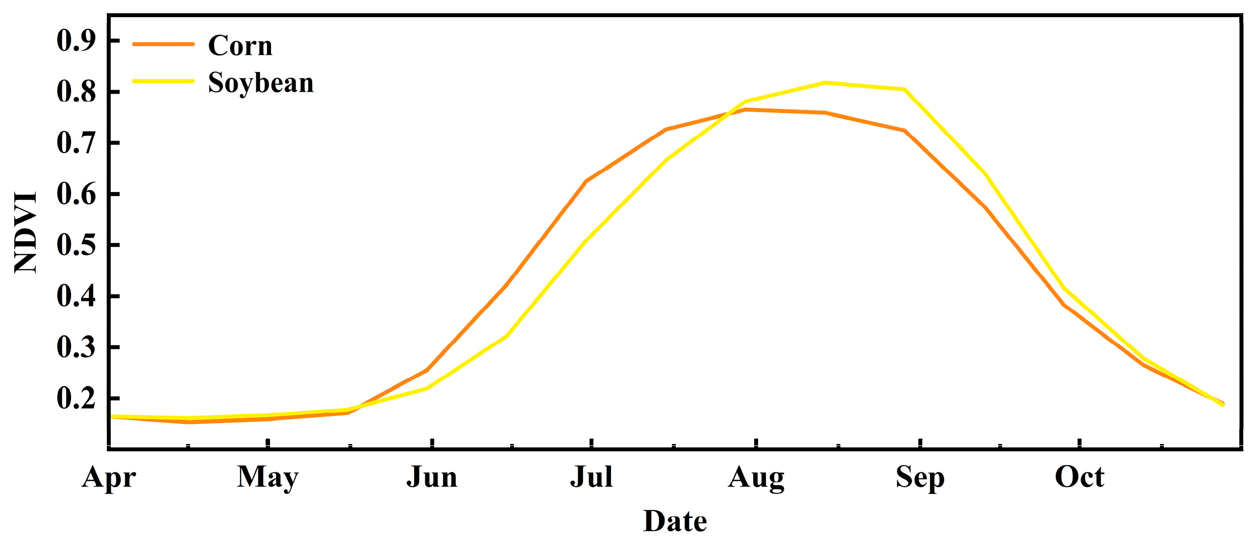
Corn and soybean are the two dominant dryland crops in the study area and frequently exhibit similar seasonal growth dynamics. To provide a general characterization of their phenological relationship, NDVI time series were extracted from representative corn and soybean samples during the 2019 growing season using Sentinel-2 observations. The resulting trajectories were smoothed using a Savitzky–Golay filter to reduce short-term fluctuations and better reveal seasonal trends.

As shown in Figure 1, both crops follow comparable seasonal development patterns, including similar periods of canopy expansion, peak vegetation activity, and senescence. Although differences can be observed at certain growth stages, substantial temporal overlap is present throughout much of the growing season. This phenological similarity provides useful background information for understanding the crop discrimination challenges addressed in this study.

2.2. Multi-Source Remote Sensing and Meteorological Data Acquisition and Preprocessing

Utilizing the Google Earth Engine (GEE) cloud platform, this study integrated and preprocessed multi-source datasets covering optical, Synthetic Aperture Radar (SAR), and meteorological reanalysis data.

• Optical remote sensing data: Sentinel-2 Level-2A Surface Reflectance products from June to August 2019 were used as the primary optical data source. All available Sentinel-2 images during this period were subjected to pixel-level cloud masking using the QA60 quality assessment band, and Landsat 8 images from the same period were used as supplementary observations to reduce cloud-induced gaps. The cloud-masked observations were then aggregated using a median composite algorithm to generate one cloud-free summer optical composite image for the study area. The spatial resolution of the final optical composite was standardized to 10 m.
• Radar time-series data: Sentinel-1 Ground Range Detected (GRD) products in Interferometric Wide (IW) swath mode from May to October 2019 were selected. All available Sentinel-1 images during this period were preprocessed using standardized procedures, including orbit correction, radiometric calibration, and terrain correction. The VV and VH polarized backscatter coefficients were extracted and aggregated into monthly composites, resulting in six monthly SAR composite images from May to October. Each monthly composite retained both VV and VH polarization channels, producing six VV and six VH backscatter layers for constructing the SAR time-series feature library representing the physical structural evolution of the crop canopy.
• Meteorological reanalysis data: The ERA5-Land daily reanalysis dataset, with an original spatial resolution of 0.1° (~9–10 km), was used for the period from May to October 2019. The extracted meteorological variables included 2 m daily mean temperature, daily total precipitation, and total surface net solar radiation. To match the spatial grid of the Sentinel-based features, the ERA5-Land variables were resampled to 10 m using bilinear interpolation. It should be emphasized that this resampling was performed only for grid alignment and pixel-wise feature stacking, and should not be interpreted as physical downscaling. The interpolated meteorological variables do not represent true 10-m local meteorological variability; instead, they were used as regional environmental baseline constraints for crop growth rather than parcel-specific meteorological measurements.

2.3. Construction of Training and Validation Sample Sets

High-quality reference samples are the foundation of large-scale fine crop mapping. This study employed expert visual interpretation based on multi-source remote sensing imagery and field survey information to construct a pure-pixel sample set covering the major crop types in the study area. Sub-meter ultra-high-resolution historical imagery from Google Earth and multispectral false-color composite images from Sentinel-2 during critical growth stages were integrated during sample collection. For rice, characteristic flooding and transplanting signals observed in Sentinel-2 imagery served as important auxiliary references, whereas corn and soybean samples were primarily identified through field observations and visual interpretation of high-resolution imagery.

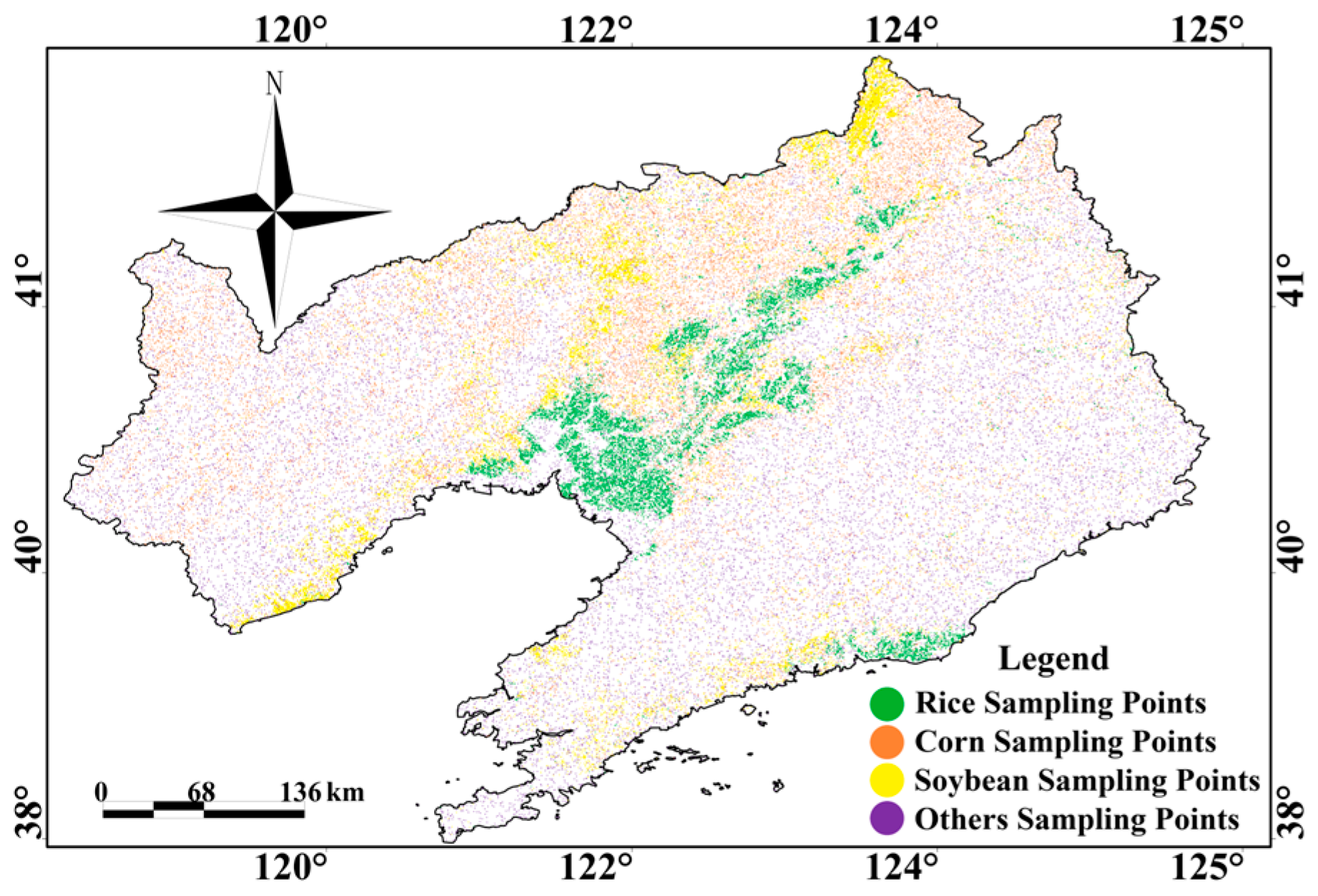
Typical parcels were selected uniformly and randomly within the study area. Homogeneous regions of interest (ROIs) located in the center of the parcels were delineated and subsequently converted into pixel-level sample points. A total of 83,254 high-quality pure pixel samples were obtained, including 20,623 for corn, 22,631 for soybean, 20,000 for rice, and 20,000 for other land cover types (e.g., forest, water, and built-up areas). The spatial distribution of sample points for each category is shown in Figure 2. All samples were randomly divided into independent training and validation sets at a ratio of 8:2, which were used for model construction and independent accuracy assessment, respectively.

3. Methodology

3.1. Technical Route

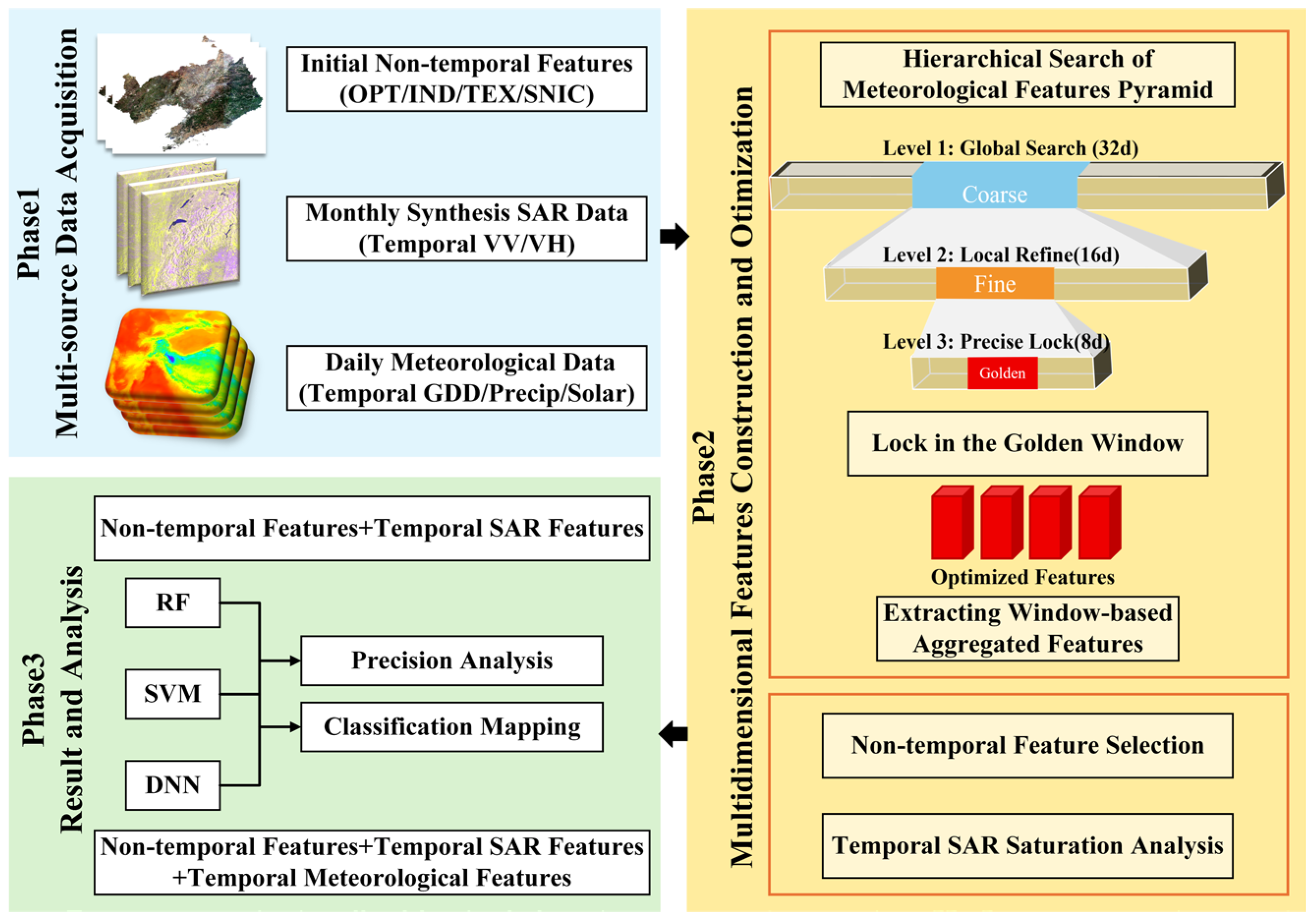
This study explores a large-scale fine crop classification method that integrates multi-source remote sensing imagery and meteorological data. The overall technical route is illustrated in Figure 3. The research framework primarily encompasses multi-source remote sensing data acquisition and preprocessing, multi-dimensional feature construction and selection, classification model training and comparison, and accuracy evaluation and fine mapping.

3.2. Construction of the Multi-Dimensional Feature Space

To comprehensively capture the phenotypic attributes and phenological evolution processes of crops, this study constructed an initial feature space integrating “spectrum–index–texture–geometry–microwave–meteorology,” with a total of 610 features.

3.2.1. Non-Time-Series Features

Non-time-series features aim to characterize the static cumulative attributes of crops during the vigorous growth period in summer (June to August). Based on the summer composite imagery, a total of 46 feature variables were extracted:

• Spectral bands and vegetation index features: Ten original spectral bands of Sentinel-2 were extracted. Based on these, ten vegetation and environmental indices covering greenness, biomass, and canopy moisture sensitivity were calculated (

  Table 1. Initial feature space.

  Feature Dimension	Feature Category	Variable Name	Quantity	Calculation Formula or Parameter Description
  Non-time-series	Spectral Band	$B_2,B_3,B_4,B_5,B_6,B_7,B_8,B_{8A},B_{11},B_{12}$	10
  	Vegetation and Environmental Index	NDVI, EVI, kNDVI, LSWI, NDWI, NBR, NDBI, NDRE1, GCVI, TCWetness	10	$kNDVI=\tanh \left(NDV{I}^2\right)$ $TCWetness=0.1509B_2+0.1973B_3+0.3279B_4+0.3406B_8-0.7112B_{11}-0.4572B_{12}$ (Other conventional index formulas are omitted)
  	Spatial Texture	Contrast, Correlation, IDM, Entropy (Based on $B_6,B_8,NDVI$)	12	The sliding window size is 3 × 3, the input source is multiplied by 100 and rounded to discretize, and the contrast, correlation, homogeneity, and entropy are extracted.
  	Object-Oriented	Geometric Features: Area, Perimeter, Width, Height, Shape Index, Compactness Statistical Features: Mean & StdDev (based on $B_2,B_3,B_4,B_8$)	14	SNIC parameters: seed spacing 15, compactness 0, neighborhood 256 $Compactness=4\mathsf{\pi }\times Area/Perimete{r}^2$
  Time-series	SAR time-series	Mon5_VV/VH to Mon10_VV/VH	12	Monthly mean synthesis, missing values interpolated with seasonal climate state
  	Meteorological time-series	Daily GDD	552	$GD{D}_i=\max \left(T_{2m,i}-273.15-T_{base},0\right)$
  		Daily Precip		Cumulative precipitation, unit conversion to $\mathrm{m}\mathrm{m}$
  		Daily Solar		Net surface solar radiation, unit conversion to $\mathrm{M}\mathrm{J}/{\mathrm{m}}^2$
  Total		Initial total number of features to be optimized	610

  ), including NDVI, EVI, LSWI, NBR, and Tasseled Cap Wetness (TCWetness), to amplify the biochemical attribute differences among different crops.
• Spatial texture features: The Gray-Level Co-occurrence Matrix (GLCM) was used to quantify the spatial arrangement patterns of the crop canopy. The red-edge band ($B_6$), near-infrared band ($B_8$), and NDVI were selected as input sources. The sliding window size was set to $3 \times 3$ pixels. Four core measures were calculated: Contrast, Correlation, Inverse Difference Moment (IDM), and Entropy.
• Object-oriented features: To suppress the “salt-and-pepper noise” in pixel-level classification, this study introduced the Simple Non-Iterative Clustering (SNIC) algorithm. Superpixel objects were constructed using $B_2$, $B_3$, $B_4$, and $B_8$ as inputs (seed spacing of 15, compactness of 0). Furthermore, 14 object-level features were extracted, including 6 geometric parameters (area, perimeter, aspect ratio, compactness, etc.) and 8 statistical parameters (mean and standard deviation of $B_2$, $B_3$, $B_4$, and $B_8$ within the object).

3.2.2. Time-Series Features

To capture the dynamic physical and physiological mechanisms during the crop growth cycle, this study further constructed microwave and meteorological time-series features:

• SAR polarization time-series features: The C-band microwave from Sentinel-1 exhibits high sensitivity to crop canopy structure and moisture content [20]. This study adopted a monthly mean composite method to extract the mean VV and VH polarized backscatter coefficients from May to October, constructing a 12-dimensional radar time-series feature set. For a few pixels with missing observations, interpolation compensation was performed using the climatological mean of the growing season.
• High-frequency meteorological time-series features: Meteorological factors are the intrinsic driving forces of crop phenological evolution [21]. Based on ERA5-Land data, this study calculated daily meteorological variables for a total of 184 days from May to October:
  • Growing Degree Days (GDD): Setting the base temperature ($T_{base}$) at 10 °C, the absolute temperature at 2 m ($T_{2m}$, unit: K) provided by ERA5 was converted to degrees Celsius, and the base temperature was subtracted. Values below 0 were truncated to 0 to calculate the effective heat accumulation:

    $$GD{D}_i=\max \left(T_{2m,i}-273.15-T_{base},0\right)$$

    (1)

    where $i$ denotes the specific observation date.
  • Daily Precipitation (Precip): The daily total precipitation ($P_{sum}$, original unit: m) from ERA5-Land was extracted and converted into standard meteorological units (mm).
  • Daily Net Solar Radiation (Solar): The total surface net solar radiation ($R_{net}$, original unit: $\mathrm{J}/{\mathrm{m}}^2$) was extracted and standardized to megajoules per square meter ($\mathrm{MJ}/{\mathrm{m}}^2$) to optimize model convergence.

The finally constructed 610-dimensional feature space is summarized in Table 1.

3.3. Feature Selection

In fine crop classification using multi-source feature fusion, although extracting high-dimensional features can describe land cover attributes from multiple perspectives, it also increases the computational burden, introduces redundant information and collinearity noise, and triggers the curse of dimensionality [22]. Therefore, performing dimensionality reduction and feature selection on high-dimensional feature sets prior to model training is a critical step to improve model generalization capability and mitigate overfitting.

3.3.1. Non-Time-Series Feature Selection

Targeting the 46 non-time-series features extracted in Section 3.2.1, this study employed a filter feature selection algorithm based on the F-statistic (F-score) for optimization. The F-score is a simple and highly robust feature evaluation criterion widely used to assess the discriminative ability of individual features for target classes [23]. Its core idea is to measure the classification contribution of a feature by quantifying the ratio of its between-class variance to within-class variance. If a feature exhibits a large between-class variance among different crop categories and a small within-class variance within the same category, its F-score is higher, indicating a stronger separability for crop categories.

Given a training sample set, assuming there are $K$ classes, the F-score of the $i$-th feature is calculated as follows:

$$F\left(i\right)={\displaystyle \frac{{\sum }_{k=1}^K{n}_k{\left(\overline{x_i^{\left(k\right)}}-\overline{x_i}\right)}^2}{{\sum }_{k=1}^K\frac{1}{n_k-1}{\sum }_{j=1}^{n_k}{\left(x_{i,j}^{\left(k\right)}-\overline{x_i^{\left(k\right)}}\right)}^2}}$$

(2)

where $\overline{x_i}$ is the average value of the $i$-th feature across all samples; $\overline{x_i^{\left(k\right)}}$ is the average value of the $i$-th feature in the $k$-th class of crop samples; $n_k$ is the number of samples in the $k$-th class; and $x_{i,j}^{\left(k\right)}$ represents the value of the $j$-th sample in the $k$-th class on the $i$-th feature. The numerator represents the between-class variance, and the denominator represents the within-class variance.

Traditional feature selection methods often require the number of retained features to be specified in advance, which may introduce subjectivity into the selection process. Motivated by the marginal utility and peaking phenomenon in feature selection [24], this study employed a marginal-gain-based adaptive truncation strategy to determine the optimal non-time-series feature subset.

After calculating the F-score values, all candidate non-time-series features were ranked in descending order according to their discriminative ability. Rather than relying on a predefined empirical threshold, the method evaluates the overall shape of the ranked marginal-gain curve. By iteratively tracking the individual F-score contribution and marginal gain of each newly introduced feature, the truncation point is determined according to the transition from the information-rich region to a sustained low-contribution region. Beyond this transition point, additional features provide progressively diminishing gains while increasing feature redundancy and model complexity. Therefore, only the features preceding the onset of the low-contribution region are retained for subsequent analysis.

3.3.2. Time-Series Feature Selection

• Information saturation assessment of SAR polarization time-series features

To accurately characterize the growth cycle and phenological transition points of crops, temporally continuous observation sequences are required [25]. Direct truncation of SAR features from specific months may disrupt the phenological continuity of crop development and lead to the loss of structural information during critical growth stages. Therefore, for the 12-dimensional polarization time-series features from May to October, this study did not directly apply the marginal-benefit truncation strategy used for static features. Instead, an information saturation assessment was conducted to determine whether temporal truncation was necessary for the SAR polarization sequence.

The purpose of this assessment was not to enforce feature elimination, but to evaluate whether the cumulative classification contribution of the SAR polarization time-series features exhibited an early saturation pattern [26]. If the cumulative contribution reached a stable plateau before all temporal features were included, partial truncation could be considered. Conversely, if no clear early saturation point was observed, retaining the complete seasonal sequence would be more appropriate for preserving phenological continuity and complementary structural information. Therefore, this assessment provided a data-driven basis for deciding whether the full growing-season SAR time-series features should be retained or partially truncated in the subsequent multi-source fusion model.

2.

Pyramid multi-scale sliding window selection of high-frequency meteorological time-series features

The 552 daily meteorological features extracted in Section 3.2.2 cannot be directly used without selection, because they may increase dimensionality and obscure key meteorological signals with temporal background noise. From an agronomic perspective, the phenological evolution and canopy spectral variation in crops are controlled by local short-term climatic forcing [21]. The stress or promotion responses of different crops to environmental factors have specific temporal limitations. Traditional fixed-period composition methods (e.g., monthly or dekadal) are prone to the boundary truncation effect, which may sever the true phenologically sensitive periods [27].

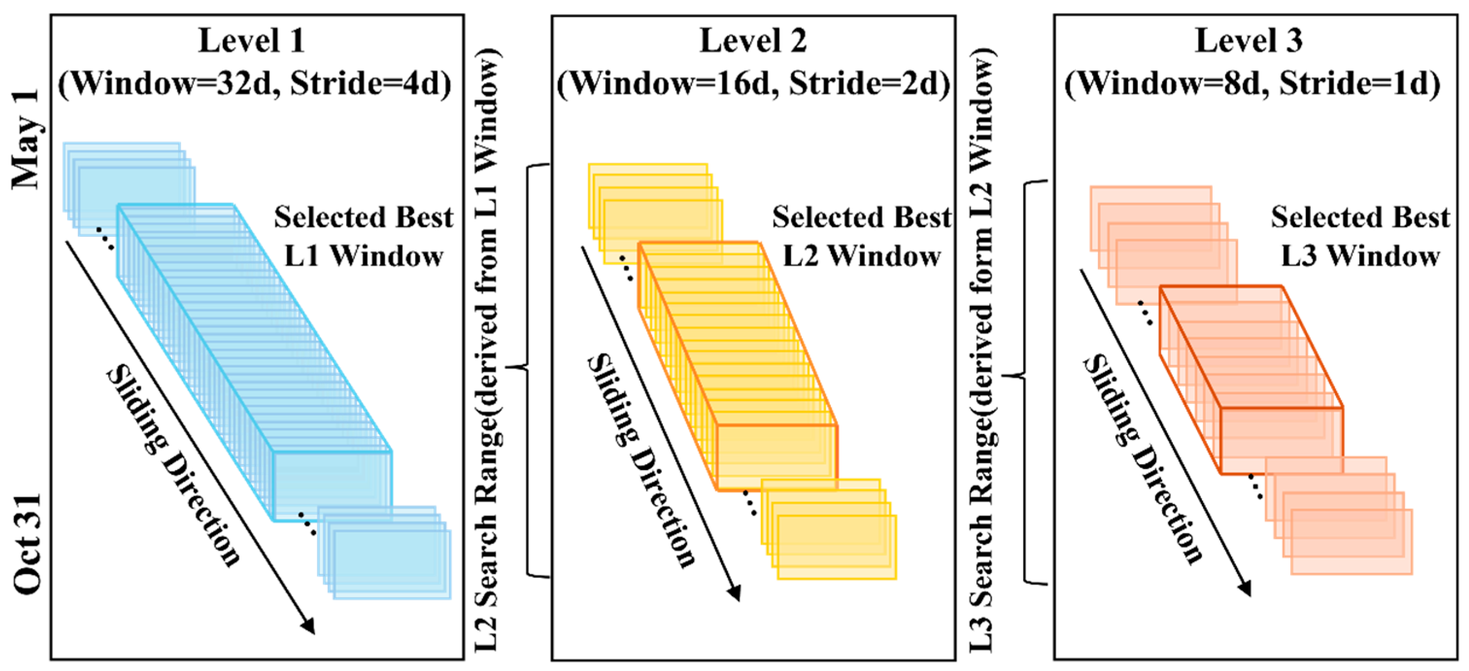
To locate the phenologically sensitive windows of crops in continuous time series, inspired by the hierarchical sub-window search framework in computer vision [28] and the incremental sliding feature weighting method [29], this study constructed an agronomy-oriented Pyramid Multi-scale Sliding Window time-series selection algorithm (Figure 4). The algorithm was applied independently to each daily meteorological variable, including GDD, precipitation, and solar radiation. For each candidate window, the mean value within the window was calculated as the corresponding window-level meteorological feature, and its inter-class discriminability was evaluated using the penalized F-score described below.

In the multi-scale evaluation, longer time windows may accumulate greater absolute inter-class differences, causing the algorithm to favor larger windows during the hierarchical search. To reduce this scale-induced bias, this study introduced a Temporal Scale Penalty into the objective function, which divides the F-score of each candidate window by the square root of the window length ($W_{size}$):

$$Scor{e}_{window}={\displaystyle \frac{F_{val}}{\sqrt{W_{size}}}}$$

(3)

This penalty mechanism mathematically constrains the algorithm to search for agronomically sensitive burst periods with short time spans but concentrated classification information, ensuring that the identified 8-day window has high information density.

After locating the core 8-day window, considering the high sensitivity of crop phenological development to short-term climatic forcing, calculating only the overall mean of a long window easily produces a temporal smoothing effect [30]. This effect can filter out key abrupt meteorological signals, such as concentrated precipitation or short-term heat stress. To preserve the temporal heterogeneity within the core window, this study performed a “high-frequency slicing” reconstruction on the 8-day window: using a 2-day step, the window was consecutively divided into 4 micro-time-steps, generating 4 two-day composite features, respectively.

3.3.3. Separability Analysis

After completing the non-time-series feature truncation and meteorological time-series feature selection, to quantitatively evaluate the actual discriminative ability of the retained core feature subset for rice, corn, soybean, and other background land covers, this study introduced the Jeffries–Matusita (J–M) distance to conduct feature separability analysis [31].

3.4. Classification Model Construction and Accuracy Assessment

3.4.1. Classification Model Construction

In this study, the classifier input was a structured feature set composed of optical, SAR, and meteorological variables after feature construction and selection, rather than raw temporally aligned sequences. Therefore, the current experiments focused on classifiers suitable for structured feature representations, while end-to-end sequence-based deep learning architectures are discussed as future work in Section 5.3.

• Random Forest (RF): RF is an ensemble learning algorithm based on decision trees, which improves classification robustness through bootstrap sampling and random feature selection [22]. In this study, RF was used to handle the multi-source features composed of optical, SAR, and meteorological variables. The number of trees was optimized according to the validation overall accuracy, while the remaining parameters were kept as default.
• Support Vector Machine (SVM): Considering the nonlinear separability and spectral confusion between corn and soybean, an SVM classifier with the Radial Basis Function (RBF) kernel was adopted. The penalty parameter C and kernel parameter gamma were optimized using Bayesian optimization based on the validation samples [32].
• Deep Neural Network (DNN): The DNN was implemented as a lightweight multilayer perceptron to learn nonlinear relationships from the structured input features [33]. The network contained two fully connected hidden layers with 128 and 64 neurons, respectively, followed by ReLU activation functions. The output layer was connected to a softmax classification layer. The model was trained using the Adam optimizer with an initial learning rate of 0.001, a mini-batch size of 256, and a maximum of 100 epochs, and the network with the lowest validation loss was retained.

Feature extraction and spatial prediction were conducted on the Google Earth Engine platform, while local parameter tuning and DNN training were performed in MATLAB R2023a using the Statistics and Machine Learning Toolbox and the Deep Learning Toolbox. For RF and SVM, hyperparameters were independently optimized for each feature input scheme using the same training–validation split and model-selection criterion. The DNN was trained on a CPU-based local workstation without GPU acceleration.

3.4.2. Classification Experimental Design

To quantitatively evaluate the gain of meteorological time-series features on crop classification accuracy, this study adopted an ablation study strategy and designed two sets of feature input schemes. Under the premise of fixing training samples and classifier hyperparameters, the experimental design is as follows:

• Scheme I: Baseline feature combination. The input space contains the optimized optical features and time-series microwave features. This combination comprehensively utilizes optical data to capture biochemical attributes and synergizes with SAR time-series data to characterize canopy structural evolution, constituting the classification baseline for current conventional large-scale crop mapping.
• Scheme II: Multi-source fusion feature combination. Building upon the baseline combination, the optimally extracted high-frequency meteorological time-series features were introduced. This scheme aims to verify whether introducing meteorological factors as physiological constraints can effectively weaken the spectral confusion (i.e., inter-class spectral similarity and intra-class variability) in the high-dimensional feature space, thereby improving the identification accuracy of highly confused dryland crops.

3.4.3. Classification Accuracy Assessment

Classification accuracy assessment is a core step in verifying the effectiveness of multi-source feature selection and the generalization ability of the models. Based on an independent validation set, this study constructed a confusion matrix as the foundational statistical tool for accuracy assessment [20]. To comprehensively and objectively quantify the identification performance of the classifiers, this study followed the standard evaluation system for large-scale remote sensing mapping [34] and selected four core metrics for comprehensive evaluation: Overall Accuracy (OA), Producer’s Accuracy (PA), User’s Accuracy (UA), and the Kappa coefficient.

4. Results and Analysis

4.1. Feature Selection Results

4.1.1. Results of Non-Time-Series Feature Selection

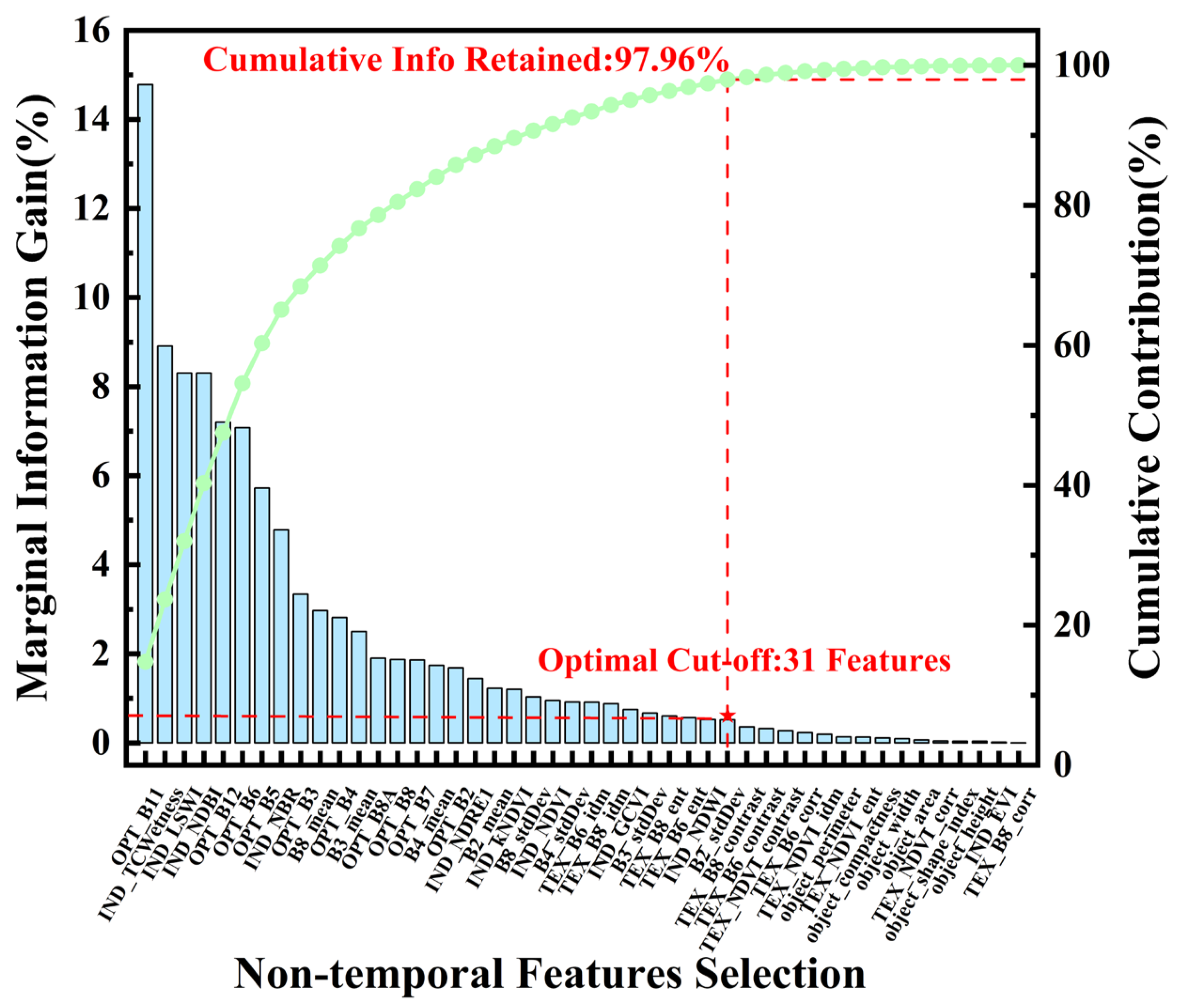
For the 46-dimensional non-time-series features initially extracted, this study performed dimensionality reduction using the F-statistic and marginal-gain-based adaptive truncation strategy. Based on the marginal-gain analysis, the F-score contributions of the extracted variables were evaluated (Figure 5). The ranked marginal-gain curve exhibited a distinct transition around the 31st feature. Specifically, the marginal gain of the 31st feature was 0.5238%, whereas that of the 32nd feature declined sharply to 0.3597%, corresponding to a reduction of approximately 31.3%. Beyond this point, the curve entered a sustained low-contribution region characterized by progressively diminishing gains. This pattern indicates that the first 31 features captured the majority of discriminative information, with a cumulative retained effective classification information of 97.96%, whereas subsequent variables provided substantially lower incremental contributions. Accordingly, the feature space was truncated based on the observed transition pattern of the marginal-gain curve, resulting in a compact subset of 31 non-time-series features and eliminating 15 low-contribution variables.

4.1.2. Results of Time-Series Feature Selection

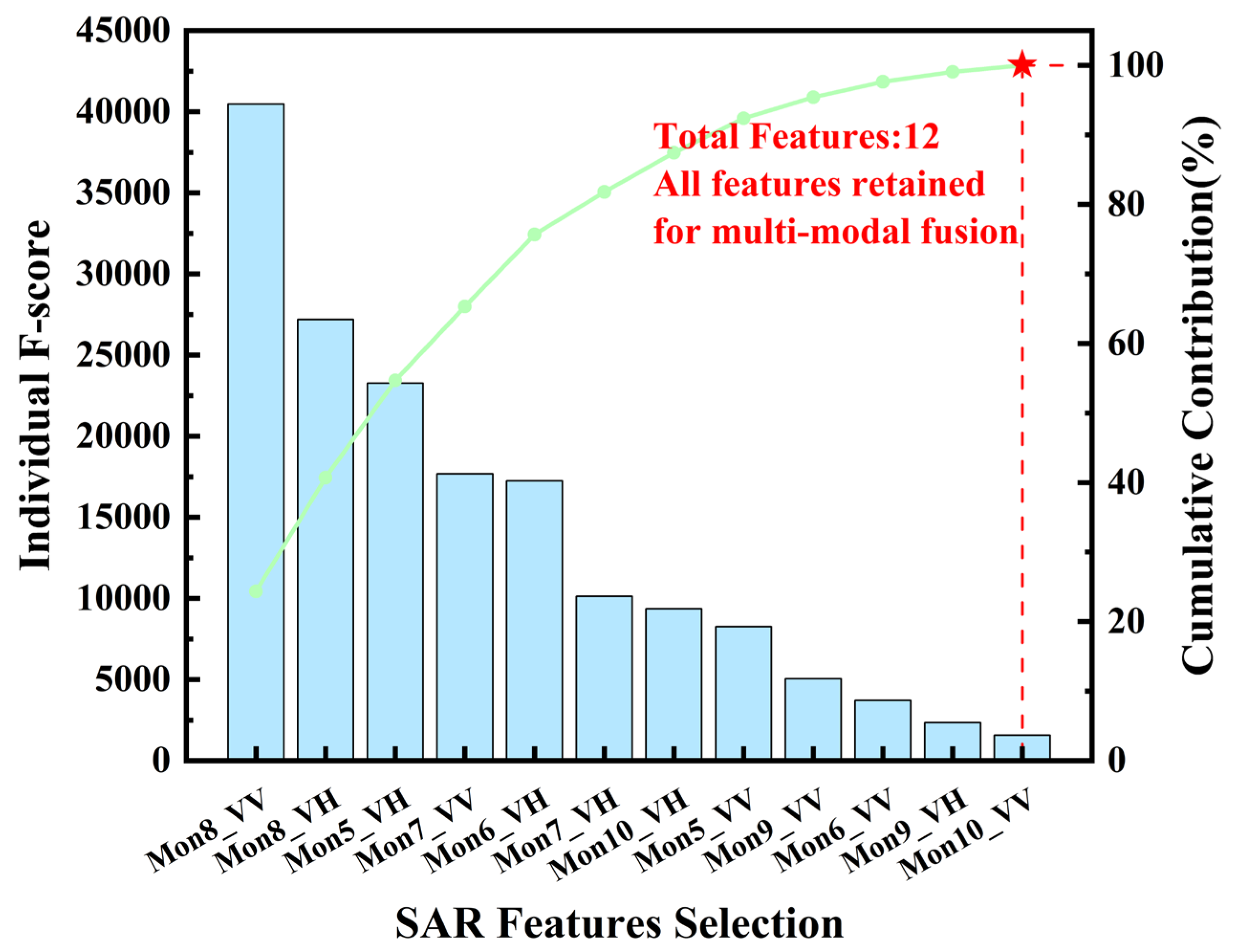
• Information saturation assessment of SAR polarization time-series features: An information saturation assessment was conducted on the 12-dimensional polarization time-series features covering the entire crop growing season. As shown in Figure 6, the cumulative classification contribution continued to increase as the ranked SAR polarization features were progressively included, and no clear early saturation point or stable plateau was observed before the complete 12-dimensional feature set was incorporated. This result indicates that the SAR polarization time-series features provide complementary structural information related to crop phenological development. Therefore, threshold-based temporal truncation was not applied to the SAR time-series features, and the complete 12-dimensional SAR polarization time-series feature set was incorporated into the multi-source feature space.
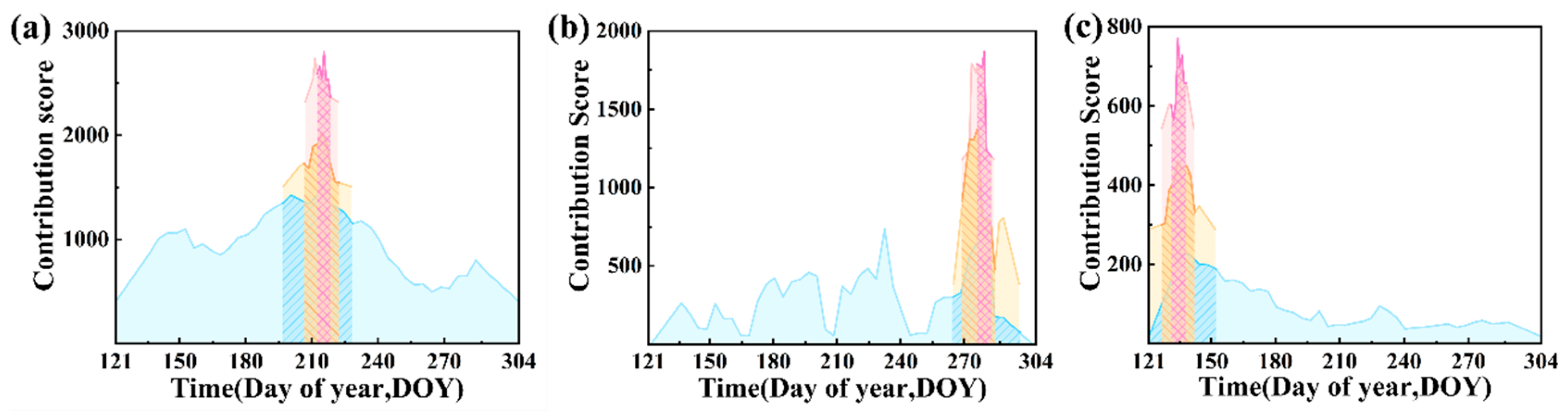
• Results of meteorological time-series feature selection: The pyramid multi-scale sliding window algorithm was utilized to filter the 552-dimensional daily meteorological variables, ultimately extracting 12 core meteorological slices (Figure 7). The target contribution of GDD exhibited a stepwise jump as the search level progressed, ultimately locking the 212th to 219th days as the core window. The peak of Precip was precisely locked between the 276th and 283rd days. Meanwhile, the optimized peak of Solar was concentrated in the early stage of crop growth, from the 131st to 138th days.

After feature selection, this study obtained an optimized multi-source feature space integrating optical phenotypic, SAR structural, and meteorological features. The specific physical attributes and classification roles of each feature are detailed in

Table 2. Summary of the optimized multi-source feature combination.

Feature Dimension	Feature Subclass	Specific Feature Variable Name	Quantity
Non-time-series features	Spectral Band	$B_2,B_3,B_4,B_5,B_6,B_7,B_8,B_{8A},B_{11},B_{12}$	10
	Vegetation and Environmental Index	TCWetness, LSWI, NDBI, NBR, NDRE1, kNDVI, NDVI, GCVI, NDWI	9
	Spatial Texture	$B_{6\_idm},B_{8\_idm},B_{6\_ent},B_{8\_ent}$	4
	Object-Oriented	${B_2}_{\mathrm{IDM}},{B_3}_{\mathrm{Mean}},{B_4}_{\mathrm{Mean}},{B_8}_{\mathrm{Mean}},$ ${B_2}_{\mathrm{StdDev}},{B_3}_{\mathrm{StdDev}},{B_4}_{\mathrm{StdDev}},{B_8}_{\mathrm{StdDev}}$	8
Time-series features	SAR time-series	Mon5_VV, Mon5_VH, Mon6_VV, Mon6_VH, Mon7_VV, Mon7_VH, Mon8_VV, Mon8_VH, Mon9_VV, Mon9_VH, Mon10_VV, Mon10_VH	12
	Meteorological time-series	GDD_DOY212_2d, GDD_DOY214_2d, GDD_DOY216_2d, GDD_DOY218_2d, Precip_DOY276_2d, Precip_DOY278_2d, Precip_DOY280_2d, Precip_DOY282_2d, Solar_DOY131_2d, Solar_DOY133_2d, Solar_DOY135_2d, Solar_DOY137_2d	12
Total		Total number of features after selection	55

.

4.1.3. Separability Evaluation of Optimized Features

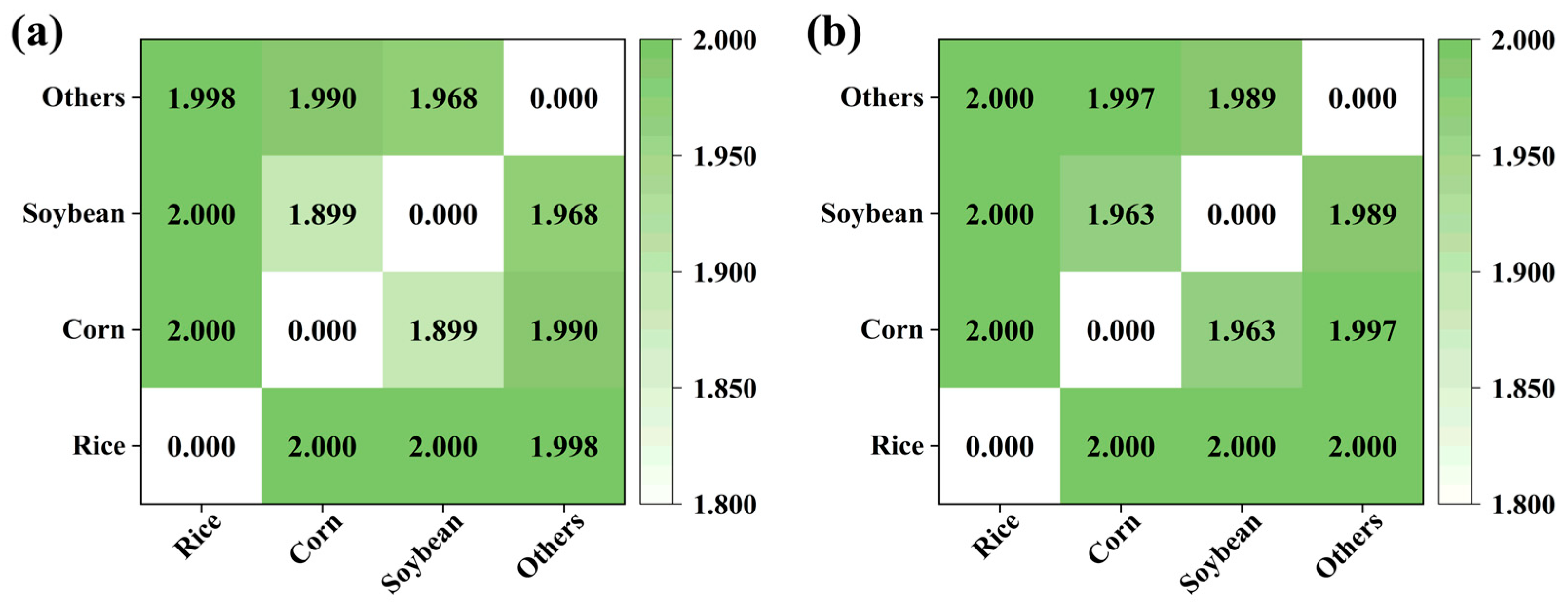
Based on the Jeffries–Matusita (J–M) distance, this study quantitatively evaluated the discriminative capability of both the baseline feature combination and the multi-source fusion feature combination (Figure 8). The results indicated that all off-diagonal J–M distances exceeded 1.89, suggesting a generally high degree of separability among the four land-cover categories.

Compared with the baseline feature combination, the multi-source fusion feature combination generally achieved higher J–M distances between several category pairs. In particular, the J–M distance between corn and soybean increased from 1.899 to 1.963 after the incorporation of the selected meteorological variables. Smaller improvements were also observed between corn and others (1.990–1.997) and between soybean and others (1.968–1.989). Rice maintained near-perfect separability from the remaining categories, with J–M distances approaching the theoretical maximum value of 2.00.

These results suggest that the optimized meteorological variables provide complementary information beyond optical and SAR features, contributing to improved separability among crop categories in the feature space. The enhanced separability between corn and soybean is consistent with the classification performance improvements reported in the subsequent accuracy assessment.

4.2. Classification Results and Analysis

Before comparing the classification accuracies, the optimized model parameters used for the final prediction are summarized in

Table 3. Optimized model parameters used for final classification.

Classifier	Common Model Settings	Baseline Feature Combination	Multi-Source Fusion Feature Combination
RF	Trees selected by validation OA; other parameters default	150 trees	500 trees
SVM	RBF kernel; C and gamma optimized by Bayesian optimization	C = 980.0179; gamma = 1.0 × 10−5	C = 965.8612; gamma = 0.0008
DNN	MLP: 128–64 hidden neurons; ReLU; Adam; lr = 0.001; batch = 256; epochs = 100; best validation-loss model retained	Input = 43	Input = 55

. These parameters were obtained from the model-selection procedure described in Section 3.4.1 and were subsequently used for accuracy assessment and spatial mapping.

4.2.1. Classification with the Baseline Feature Combination

This study constructed a baseline combination space containing the optimized optical features and microwave time-series features, serving as a classification baseline representing the conventional configuration of “optical combined with radar.” Based on this feature set, comprehensive performance evaluations were conducted using Random Forest (RF), Support Vector Machine (SVM), and Deep Neural Network (DNN) (

Table 4. Accuracy evaluation of different classification algorithms based on the baseline features.

Model	Category	PA/%	UA/%	OA/%	Kappa
RF	Rice	97.35	96.72	89.91	0.8653
	Corn	86.64	88.33
	Soybean	90.50	87.33
	Others	85.19	87.62
SVM	Rice	97.25	96.86	90.45	0.8725
	Corn	88.19	89.30
	Soybean	90.81	88.54
	Others	85.56	87.33
DNN	Rice	98.00	95.63	90.14	0.8683
	Corn	86.32	91.38
	Soybean	92.66	86.56
	Others	83.36	87.52

).

• Overall performance: Based on the baseline feature combination, the SVM model achieved the best performance among the three classifiers, with an OA of 90.45% and a Kappa coefficient of 0.8725. The DNN achieved an OA of 90.14% and a Kappa coefficient of 0.8683, indicating that the lightweight MLP architecture could capture useful nonlinear relationships from the optical–SAR feature set. The RF model reached an OA of 89.91%, showing stable but slightly lower performance under the baseline feature configuration.
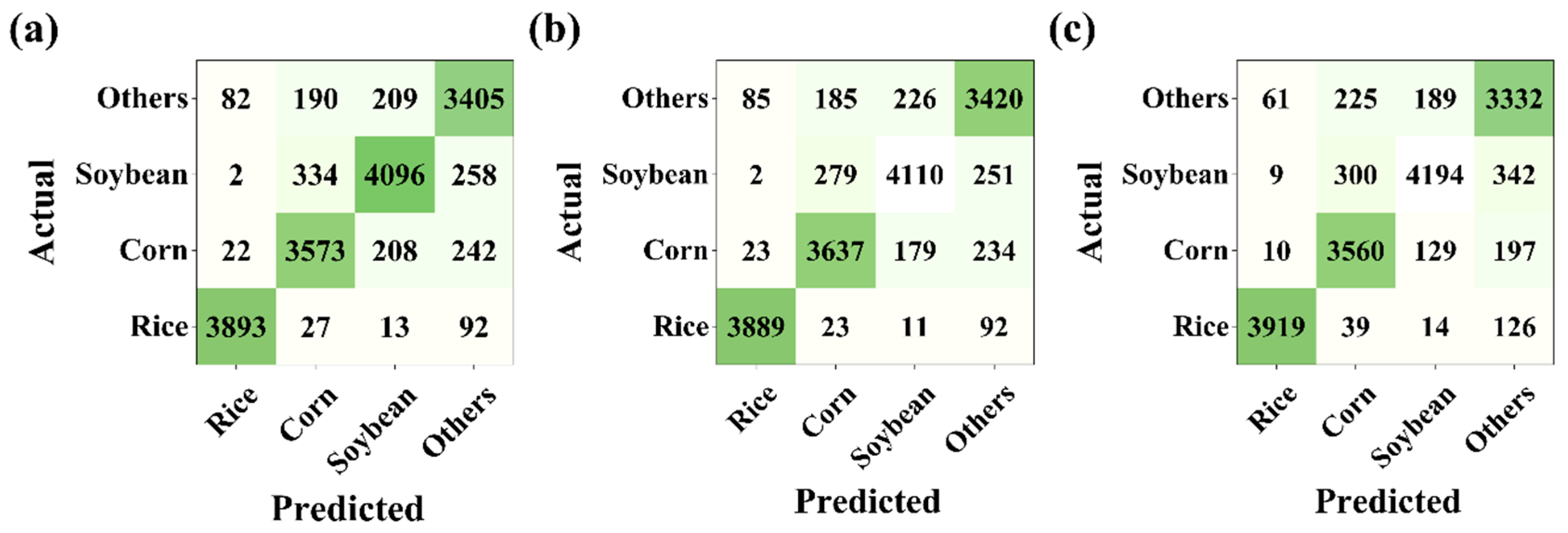
• Confusion matrix analysis: The classification confusion matrices showed that all three models achieved high identification accuracy for rice, with both PA and UA exceeding 95% (Figure 9), confirming the effectiveness of the baseline optical-SAR features in capturing flooding signals and low-backscatter characteristics of rice. However, the baseline feature space still showed limitations in separating dryland crops. For corn and soybean, the PA/UA values were 86.64%/88.33% and 90.50%/87.33% for RF, 88.19%/89.30% and 90.81%/88.54% for SVM, and 86.32%/91.38% and 92.66%/86.56% for DNN, respectively. These results indicate that the main residual errors were concentrated in the bidirectional confusion between corn and soybean, especially reflected by the relatively low PA of corn and UA of soybean. This confirms that optical phenotypic and SAR structural features alone were insufficient to fully distinguish the two dryland crops with similar summer canopy characteristics.
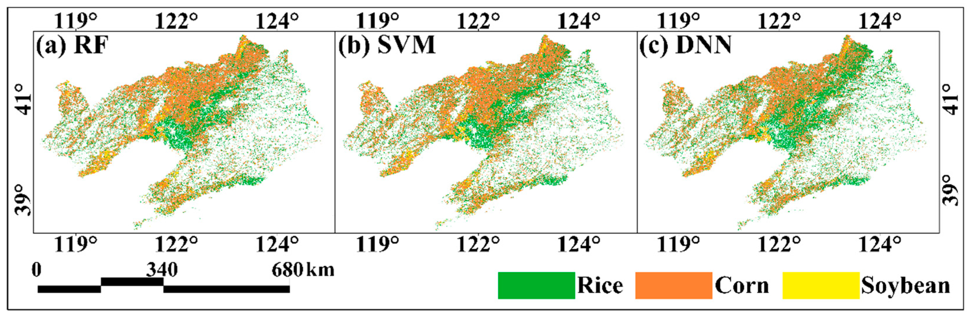
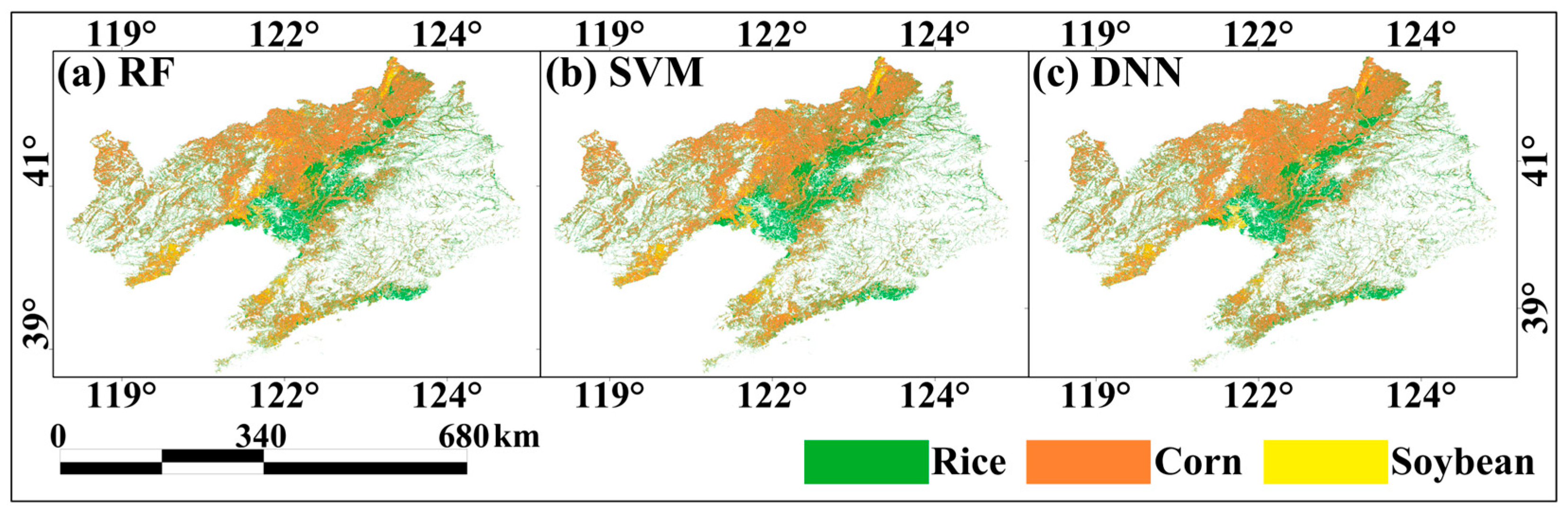
• Spatial mapping assessment: The macroscopic spatial classification mapping showed that all three models could effectively reflect the agricultural geographical distribution pattern of the study area (Figure 10). However, in local details, limited by the spectral similarity of dryland crops, the interlaced planting areas of corn and soybean exhibited obvious patch-mixing phenomena. The mapping results indicated that it is difficult to achieve high-precision unmixing of complex dryland crops relying solely on conventional optical phenotypic and radar structural features, making the introduction of environmental constraint factors capable of characterizing micro-growth rhythm differences necessary.

4.2.2. Classification with the Multi-Source Fusion Feature Combination

To explore the role of meteorological factors in weakening crop classification confusion, this study introduced the optimized 12-dimensional high-frequency meteorological time-series features based on the baseline model, and evaluated the classification performance of the multi-source fusion feature combination (

Table 5. Accuracy evaluation of different classification algorithms based on the multi-source fusion feature combination.

Model	Category	PA/%	UA/%	OA/%	Kappa
RF	Rice	97.85	96.81	90.67	0.8754
	Corn	87.39	89.47
	Soybean	91.87	87.98
	Others	85.51	88.78
SVM	Rice	98.32	96.92	91.80	0.8905
	Corn	90.37	90.24
	Soybean	92.75	90.05
	Others	85.66	90.18
DNN	Rice	98.05	96.91	91.46	0.8860
	Corn	90.32	89.59
	Soybean	92.42	89.61
	Others	84.94	89.96

).

• Overall performance: After introducing meteorological variables, the overall accuracies of all three classifiers improved. The SVM model achieved the best performance, with an OA of 91.80% and a Kappa coefficient of 0.8905. Compared with the baseline feature combination, the SVM OA increased by 1.35 percentage points. The DNN achieved an OA of 91.46% and a Kappa coefficient of 0.8860, while the RF model reached an OA of 90.67%. These results indicate that the selected meteorological variables provided complementary information to the optical–SAR feature set.
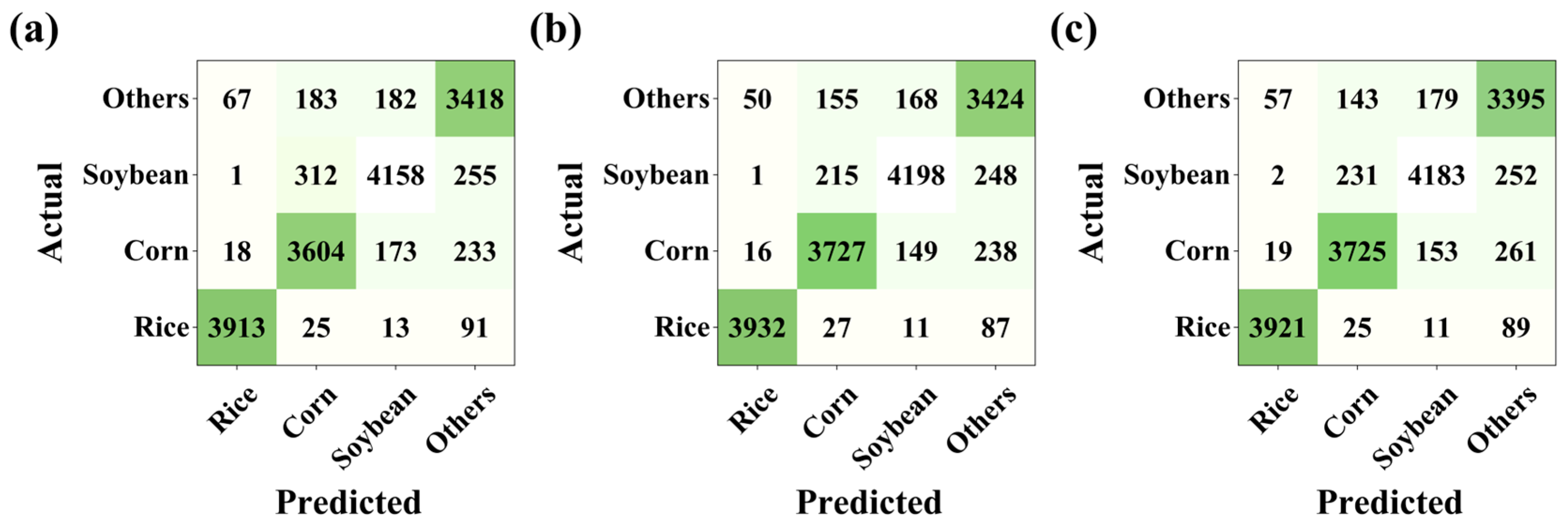
• Confusion matrix analysis: Compared with the baseline results, the introduction of meteorological time-series features reduced the confusion between corn and soybean (Figure 11). For RF, the PA/UA of corn increased by 0.75/1.14 percentage points, and those of soybean increased by 1.37/0.65 percentage points. For the optimal SVM model, the PA/UA of corn increased from 88.19%/89.30% to 90.37%/90.24%, with gains of 2.18/0.94 percentage points, while those of soybean increased from 90.81%/88.54% to 92.75%/90.05%, with gains of 1.94/1.51 percentage points. For DNN, the PA of corn and UA of soybean increased by 4.00 and 3.05 percentage points, respectively, although slight decreases occurred in corn UA and soybean PA. These crop-specific changes demonstrate that meteorological variables reduced both omission and commission errors for the two targeted dryland crops, particularly in the SVM model. This result confirms that high-frequency meteorological features provide effective physiological constraints for separating corn and soybean, whose optical and microwave responses are highly similar during the main growing season [35].
• Spatial mapping assessment: The spatial distribution results of crops in Liaoning Province at 10-m resolution based on the multi-source fusion feature combination demonstrated (Figure 12) that the introduction of meteorological factors effectively improved the classification quality in complex dryland interlaced areas. In the northwestern Liaoning and central Liaohe Plain regions, crop parcels showed improved spatial consistency, and misclassified or fragmented patches in the interlaced zones of corn and soybean were reduced. This multi-source feature space not only improved the overall statistical accuracy but also more accurately restored the geographical distribution characteristics of regional crops at the spatial scale.

4.2.3. Assessment of Spatial Classification Details

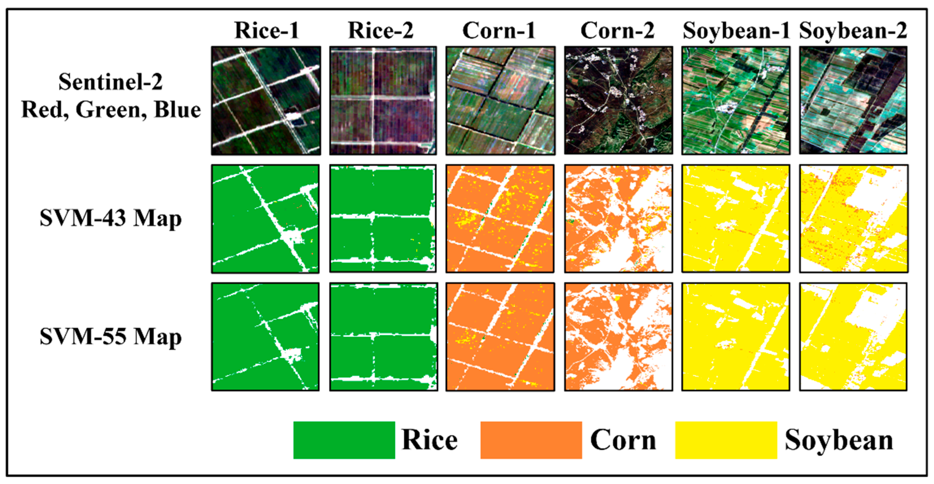
Typical planting regions of rice, corn, and soybean were selected to compare the spatial classification details of the optimal SVM model (Figure 13). The first row shows the Sentinel-2 true-color images, the second row shows the baseline classification results based on the 43-feature optical–SAR feature set, and the third row shows the classification results based on the multi-source fusion feature combination after adding meteorological variables. This comparison was designed to visually examine whether the introduction of meteorological features improved local parcel integrity and reduced the confusion between corn and soybean.

To further support the visual comparison in Figure 13, a targeted local quantitative validation was conducted for the corn and soybean sub-regions, where crop confusion was most prominent. A total of 255 validation samples were constructed by combining field survey information and manual visual interpretation. The reference labels were determined based on ground sampling records, high-resolution Google Earth imagery, and Sentinel-2 true-color and false-color composites. The samples were selected from visually homogeneous field interiors, while boundary pixels, mixed pixels, roads, water bodies, and ambiguous locations were excluded. The same sample points were used to evaluate both the baseline 43-feature classification and the fused 55-feature classification. Therefore, this analysis provides a paired local comparison of corn–soybean separability under the two feature schemes.

As shown in

Table 6. Targeted local validation of corn–soybean confusion in the sub-regions shown in Figure 13.

Region	Samples	SVM-43		SVM-55		Accuracy Gain	Confusion Reduction
		Accuracy	Confusion	Accuracy	Confusion
Corn-1	78	33.3%	65.4%	76.9%	23.1%	43.6%	42.3%
Corn-2	52	46.2%	53.8%	90.4%	9.6%	44.2%	44.2%
Soybean-1	62	80.6%	19.4%	93.5%	6.5%	12.9%	12.9%
Soybean-2	63	76.2%	23.8%	92.1%	7.9%	15.9%	15.9%

Note: confusion denotes corn samples classified as soybean or soybean samples classified as corn. This targeted validation was designed to assess the relative reduction in corn–soybean confusion in the local regions shown in Figure 13, rather than to replace the independent accuracy assessment for the entire study area.

, the fused 55-feature set consistently improved the local classification accuracy and reduced corn–soybean confusion in all four validation regions. The improvement was particularly evident in the two corn regions. In Corn R1 and Corn R2, the baseline accuracies were only 33.3% and 46.2%, respectively, indicating that a large proportion of corn samples were misclassified as soybean when only optical and SAR features were used. After incorporating meteorological features, the accuracies increased to 76.9% and 90.4%, while the corn–soybean confusion rates decreased from 65.4% and 53.8% to 23.1% and 9.6%, respectively. In the two soybean regions, the baseline accuracies were relatively higher, but the fused feature set still improved the accuracies from 80.6% and 76.2% to 93.5% and 92.1%, respectively. These results quantitatively confirm that the meteorological features effectively reduced the local corn–soybean confusion observed in Figure 13.

In the rice planting regions, both feature schemes produced generally continuous paddy fields, but the fused feature set further reduced local salt-and-pepper noise and dryland-crop misclassification within paddy areas. In the corn and soybean regions, the baseline classification showed more evident bidirectional confusion, leading to fragmented parcels and local omission errors. After incorporating meteorological features, these local misclassification patterns were reduced, and the spatial continuity of corn and soybean parcels was improved.

The targeted validation in Table 6 supports this visual interpretation. The fused 55-feature set improved the classification accuracy in all four corn–soybean validation regions and reduced the corresponding confusion rates. Although this local validation does not replace the independent accuracy assessment for the entire study area, it provides additional evidence that the selected meteorological features helped improve corn–soybean separability in representative heterogeneous planting areas.

5. Discussion

5.1. Classification Contribution and Agronomic Mechanism Analysis of Multi-Source Features

The multi-source feature selection scheme constructed in this study exhibits high consistency at the levels of physical mechanisms and agronomic logic. The dominance of the shortwave infrared (SWIR) bands among non-time-series features stems from their high sensitivity to vegetation canopy moisture content and soil background moisture. This sensitivity effectively quantified the physical moisture differences between flooded rice and dryland crops, providing a physical basis for crop unmixing in complex farmland landscapes [1]. Simultaneously, completely retaining the 12-dimensional SAR polarization features helped maintain the temporal topological logic of crop phenological evolution; by capturing the differences in 3D canopy structures of crops during critical growth stages, we enhanced classification stability under complex environments [36].

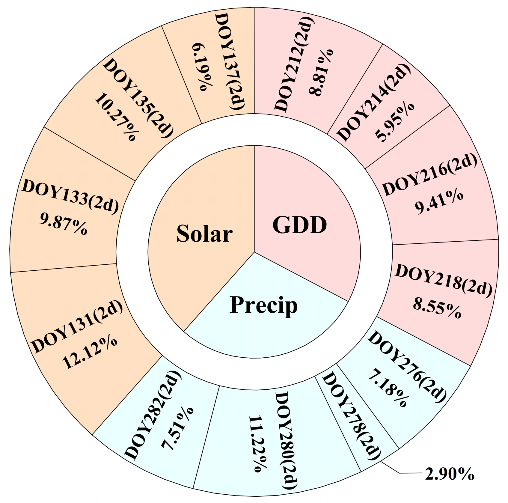
Building upon optical and microwave data, this study further introduced effective accumulated temperature, precipitation, and shortwave radiation, expanding the environmental observation dimensions. The feature importance evaluation indicated (Figure 14) that different meteorological factors played differentiated roles in fine identification. In the global feature contribution, the shortwave radiation in mid-May (Solar_DOY131_2d; approximately 11 May) ranked first in weight. The physical basis for this result is that mid-May corresponds to the rice transplanting stage and the sowing-to-emergence stage of corn and soybean in the study area. Different surface states, such as bare soil, water bodies, and primary vegetation canopies, have essential physical differences in their absorption rates of solar shortwave radiation, thereby providing a key energy balance criterion in the early stage of classification. Secondly, the importance of the precipitation feature in early October (Precip_DOY280_2d; approximately 7 October) originates from the late maturity and harvesting period of major crops in the study area. After rainfall, exposed soil and withered stubble have different response mechanisms in water infiltration and surface runoff, effectively characterizing the surface heterogeneity in the late harvesting period. In addition, the effective accumulated temperature series in early August (GDD_DOY216_2d; approximately 4 August) also exhibited a high contribution, reflecting the core driving role of heat accumulation during the tasseling–silking stage of corn and the flowering–pod initiation stage of soybean.

The distribution of these feature weights is consistent with the phenological differences among the major crops. As a C4 plant, corn, and a C3 plant, soybean, possess highly similar canopy structures and vegetation index trajectories during the summer vegetative growth period, making it difficult for conventional remote sensing methods to effectively separate them. However, there is significant differentiation in their response thresholds to environmental forcing: corn is highly sensitive to effective accumulated temperature during the tasseling–silking period in early August, whereas soybean exhibits a stronger dependence on moisture conditions during the flowering-to-pod-initiation period occurring in the same season [35]. The optimally extracted high-frequency meteorological series captured such metabolic differences, constituting the environmental and physiological features to distinguish confused crops [37]. These results indicate that meteorological variables provide physiologically relevant information that complements optical and SAR features, thereby improving the separability of dryland crops with similar spectral and structural characteristics.

5.2. Contextual Comparison with Previous Studies and Existing Crop Mapping Products

To place our results in the context of previous crop mapping studies, we compared them with relevant studies and crop mapping products in Northeast China. However, such comparisons should be interpreted cautiously because differences in study area, mapping year, spatial resolution, crop legend, sample design, input data, classification algorithm, and validation protocol may influence the reported accuracy metrics.

You et al. [2] produced annual 10-m crop type maps for Northeast China during 2017–2019 using Sentinel-2 time-series data, agro-climate-zone-specific random forest classifiers, and optimized spectral, temporal, red-edge, SWIR, and texture features. Their product provides an important regional reference for 10-m mapping of rice, maize, and soybean in Northeast China, and explicitly used red-edge and SWIR-related features to improve maize–soybean discrimination. The reported overall accuracies ranged from approximately 0.81 to 0.87, with rice generally showing higher accuracy than maize and soybean. Liu and Wang [38] further mapped annual crop types in Northeast China from 2000 to 2020 using MODIS data, feature optimization, and random forest classification, achieving sample-based overall accuracies of 84.73–86.93% for 2017–2019 and statistics-based R² values of 0.81–0.95. Their work is particularly valuable for analyzing long-term regional crop distribution and crop type changes.

Compared with these existing products, our study has a narrower spatial and temporal scope, focusing on Liaoning Province in 2019. Therefore, it should not be regarded as a replacement for existing regional or long-term crop mapping products. Instead, this study complements previous work by integrating Sentinel-1 SAR, Sentinel-2 optical, and ERA5 meteorological variables at 10-m resolution to evaluate whether meteorological information can provide additional constraints for crop discrimination, especially for corn–soybean separation in heterogeneous agricultural landscapes.

The main quantitative evidence for the effectiveness of the proposed meteorological feature fusion strategy comes from the controlled experiments within this study, rather than from direct cross-study OA comparison. Under the same study area, reference samples, classifier, and validation protocol, the baseline optical–SAR feature set achieved an overall accuracy of 90.45%, whereas the fused feature set incorporating selected meteorological variables achieved an overall accuracy of 91.80%. The accuracies of corn and soybean also improved after introducing meteorological features, indicating that meteorological variables provided complementary information for distinguishing spectrally and structurally similar dryland crops.

5.3. Limitations and Future Prospects

Although fused meteorological features improved the overall mapping accuracy, their action mechanisms on different classifiers varied. The SVM achieved a balanced improvement across all accuracy metrics, whereas the DNN exhibited asynchronous fluctuations in the individual accuracies of some dryland categories. This phenomenon exposes the limitations of the current classification framework:

First, there are limitations in the adaptability between structured hand-crafted features and feedforward neural networks. Shallow machine learning models (such as SVM and RF) have better adaptability when processing structured tabular data extracted manually [39]. Based on the margin maximization mechanism, SVM can stably process multi-source heterogeneous features. In contrast, when processing high-density hand-crafted features, the fully connected layers of the multilayer perceptron used in this study are prone to sensitive reactions to local feature scales. Lacking temporal gating units, the network may develop collinear dependence on strongly correlated meteorological and optical features during backpropagation, leading to local overfitting of decision boundaries [40].

Second, heterogeneous data exhibit scale effects and a lack of spatial context. Although the ERA5-Land meteorological variables were resampled to 10 m to align with the Sentinel observations, their native spatial resolution remains approximately 0.1° (~9–10 km). Therefore, the resampling should be regarded as grid alignment rather than physical downscaling. The resampled meteorological variables cannot represent true 10-m local meteorological variability or parcel-specific physical measurements; instead, they provide regional environmental baseline constraints describing the general hydrothermal and radiation conditions affecting crop growth.

This scale mismatch may introduce spatial smoothing effects and pseudo-precision. One native ERA5-Land grid cell covers approximately 81–100 km², corresponding to about 0.81–1.00 million 10-m pixels. Consequently, spatially dense samples located within the same or adjacent ERA5-Land grid cells may share identical or highly similar meteorological attributes, reducing the effective spatial independence of meteorological features and introducing uncertainty near meteorological grid boundaries, heterogeneous terrain, and crop transition zones.

Nevertheless, the ERA5-Land variables were used only as auxiliary regional environmental constraints, whereas the classification was mainly driven by the 10-m optical and SAR features. The ablation experiment showed that adding meteorological features increased the optimal SVM overall accuracy from 90.45% to 91.80%, corresponding to a moderate improvement of 1.35 percentage points. The producer’s accuracies of corn and soybean increased from 88.19% to 90.37% and from 90.81% to 92.75%, respectively. These results suggest that meteorological variables provided useful complementary environmental information for distinguishing phenologically similar crops, but did not dominate the classification. Future work should incorporate station-based meteorological observations, higher-resolution gridded climate products, or physically based downscaling methods to better represent local meteorological variability and reduce cross-scale uncertainty.

Third, the current accuracy assessment relied on a conventional random 8:2 training-validation split. To evaluate the robustness of this partitioning strategy, an additional stability assessment was conducted using ten independent random seeds. The resulting overall accuracies ranged from 91.49% to 92.02%, with a mean OA of 91.80% and a standard deviation of 0.16%, indicating that the proposed framework is relatively insensitive to random sample partitioning. Nevertheless, random partitioning may not completely eliminate potential spatial autocorrelation among geographically adjacent samples. Neighboring observations often share similar spectral and environmental characteristics, which may lead to slightly optimistic accuracy estimates. Future studies should further investigate spatially explicit validation strategies, such as spatial block cross-validation, to more rigorously assess model generalization under strict spatial independence constraints.

Another limitation is that this study used classifiers based on structured features after feature construction and selection, rather than end-to-end sequence-based deep learning models. Models such as 1D temporal convolutional networks and Long Short-Term Memory (LSTM) networks may directly extract higher-order representations from raw time-series data, but they require temporally aligned input sequences and different network architectures. Future research could integrate the proposed meteorological sensitive-window strategy with these models, and further introduce spatial-context constraints such as Graph Convolutional Networks (GCNs) or spatiotemporal 3D convolutions to fuse farmland topological structures with multi-source time-series features.

6. Conclusions

Targeting the need for large-scale fine crop mapping in complex agricultural areas, this study constructed a multi-source feature space fusing optical phenotypic, microwave structural, and high-frequency meteorological features, and proposed a corresponding feature selection and classification framework. The main conclusions are as follows:

(1) The combined feature selection strategy, including marginal-gain-based adaptive truncation for non-time-series features, information saturation assessment for SAR time-series features, and pyramid multi-scale sliding-window selection for meteorological time-series features, effectively reduced the dimensionality of multi-source heterogeneous data. While eliminating redundant information and reducing computational costs, this strategy precisely extracted the phenologically sensitive windows of crops, contributing to improved spatial consistency of the classification results.

(2) High-frequency meteorological time-series features provided key physiological constraints for distinguishing corn and soybean—dryland crops with highly similar spectra and structures. Among them, shortwave radiation in mid-May, precipitation in early October, and effective accumulated temperature in mid-August contributed most significantly to the classification. These features objectively reflect the differentiated responses of crops to the hydrothermal environment during critical development stages, helping to mitigate spectral confusion in the classification feature space.

(3) Driven by the fusion of non-time-series optical, microwave time-series, and high-frequency meteorological features, the SVM exhibited excellent generalization capability in processing high-dimensional structured features, achieving an overall classification accuracy of 91.80% and a Kappa coefficient of 0.8905. Comparative evaluations indicated that, within a classification framework relying on rigorous feature engineering, classical machine learning models exhibited higher classification stability and applicability than lightweight deep learning networks.

In summary, the proposed multi-source feature fusion and adaptive selection framework alleviates the feature saturation problem of conventional optical–SAR crop classification and provides methodological support for fine-scale agricultural monitoring in heterogeneous planting areas.

References

1. Zhang, C.; Zhang, H.; Tian, S. Phenology-Assisted Supervised Paddy Rice Mapping with the Landsat Imagery on Google Earth Engine: Experiments in Heilongjiang Province of China from 1990 to 2020. Comput. Electron. Agric. 2023, 212, 108105. [Google Scholar] [CrossRef]
2. You, N.; Dong, J.; Huang, J.; Du, G.; Zhang, G.; He, Y.; Yang, T.; Di, Y.; Xiao, X. The 10-m Crop Type Maps in Northeast China during 2017–2019. Sci. Data 2021, 8, 41. [Google Scholar] [CrossRef] [PubMed]
3. Zhang, H.K.; Roy, D.P. Using the 500m MODIS Land Cover Product to Derive a Consistent Continental Scale 30m Landsat Land Cover Classification. Remote Sens. Environ. 2017, 197, 15–34. [Google Scholar] [CrossRef]
4. Wang, X.; Zhao, H.; Zhao, G.; Qu, X.; Cao, C.; Qian, J.; Fu, S.; Wang, T.; Han, H. High-Resolution Crop Mapping and Suitability Assessment in China’s Three Northeastern Provinces (2000–2023): Implications for Optimizing Crop Layout. Agronomy 2025, 15, 2587. [Google Scholar] [CrossRef]
5. Zhang, H.; Yuan, H.; Du, W.; Lyu, X. Crop Identification Based on Multi-Temporal Active and Passive Remote Sensing Images. ISPRS Int. J. Geo-Inf. 2022, 11, 388. [Google Scholar] [CrossRef]
6. Yang, Y.; Cao, S.; Lu, X.; Ping, L.; Fan, X.; Liu, M.; Yang, Q.; Liu, X. A Region-Adaptive Phenology-Aware Network for Perennial Cash Crop Mapping Using Multi-Source Time-Series Remote Sensing. Remote Sens. 2025, 17, 4011. [Google Scholar] [CrossRef]
7. Ni, R.; Tian, J.; Li, X.; Yin, D.; Li, J.; Gong, H.; Zhang, J.; Zhu, L.; Wu, D. An Enhanced Pixel-Based Phenological Feature for Accurate Paddy Rice Mapping with Sentinel-2 Imagery in Google Earth Engine. ISPRS J. Photogramm. Remote Sens. 2021, 178, 282–296. [Google Scholar] [CrossRef]
8. Zhan, P.; Zhu, W.; Li, N. An Automated Rice Mapping Method Based on Flooding Signals in Synthetic Aperture Radar Time Series. Remote Sens. Environ. 2021, 252, 112112. [Google Scholar] [CrossRef]
9. Wei, J.; Cui, Y.; Luo, W.; Luo, Y. Mapping Paddy Rice Distribution and Cropping Intensity in China from 2014 to 2019 with Landsat Images, Effective Flood Signals, and Google Earth Engine. Remote Sens. 2022, 14, 759. [Google Scholar] [CrossRef]
10. Blickensdörfer, L.; Schwieder, M.; Pflugmacher, D.; Nendel, C.; Erasmi, S.; Hostert, P. Mapping of Crop Types and Crop Sequences with Combined Time Series of Sentinel-1, Sentinel-2 and Landsat 8 Data for Germany. Remote Sens. Environ. 2022, 269, 112831. [Google Scholar] [CrossRef]
11. Zeng, L.; Wardlow, B.D.; Xiang, D.; Hu, S.; Li, D. A Review of Vegetation Phenological Metrics Extraction Using Time-Series, Multispectral Satellite Data. Remote Sens. Environ. 2020, 237, 111511. [Google Scholar] [CrossRef]
12. Jennewein, J.S.; Lamb, B.T.; Hively, W.D.; Thieme, A.; Thapa, R.; Goldsmith, A.; Mirsky, S.B. Integration of Satellite-Based Optical and Synthetic Aperture Radar Imagery to Estimate Winter Cover Crop Performance in Cereal Grasses. Remote Sens. 2022, 14, 2077. [Google Scholar] [CrossRef]
13. Chen, S.; Zhao, W.; Zhang, R.; Sun, X.; Zhou, Y.; Liu, L. Higher Sensitivity of NIRv, Rad in Detecting Net Primary Productivity of C4 Than That of C3: Evidence from Ground Measurements of Wheat and Maize. Remote Sens. 2023, 15, 1133. [Google Scholar] [CrossRef]
14. Yoo, C.; Kang, D.; Park, S. Identifying the Impact of Regional Meteorological Parameters on US Crop Yield at Various Spatial Scales Using Remote Sensing Data. Remote Sens. 2022, 14, 3508. [Google Scholar] [CrossRef]
15. Awad, B.; Erer, I. Enhancing Crop Classification with Growing Degree Days: Bridging Classical Models and Regional Generalization. Remote Sens. Lett. 2025, 16, 1315–1324. [Google Scholar] [CrossRef]
16. Turkoglu, M.O.; Ledain, S.; Aasen, H. Model-Agnostic, Temperature-Informed Sampling Enhances Cross-Year Crop Mapping with Deep Learning. arXiv 2025. [Google Scholar] [CrossRef]
17. Chen, C.; Liang, J.; Sun, W.; Yang, G.; Meng, X. An Automatically Recursive Feature Elimination Method Based on Threshold Decision in Random Forest Classification. Geo-Spat. Inf. Sci. 2025, 28, 1494–1519. [Google Scholar] [CrossRef]
18. Gorelick, N.; Hancher, M.; Dixon, M.; Ilyushchenko, S.; Thau, D.; Moore, R. Google Earth Engine: Planetary-Scale Geospatial Analysis for Everyone. Remote Sens. Environ. 2017, 202, 18–27. [Google Scholar] [CrossRef]
19. Miao, S.; Jiang, Y.; Yao, J.; Shen, F.; Zhang, Z.; Xie, Z.; Li, X.; Li, H.; Huang, J. Improved Maize Mapping Through Optimizing Spatio-Temporal Feature Selection. IEEE J. Sel. Top. Appl. Earth Obs. Remote Sens. 2026, 19, 8031–8043. [Google Scholar] [CrossRef]
20. Xue, H.; Xu, X.; Zhu, Q.; Yang, G.; Long, H.; Li, H.; Yang, X.; Zhang, J.; Yang, Y.; Xu, S.; et al. Object-Oriented Crop Classification Using Time Series Sentinel Images from Google Earth Engine. Remote Sens. 2023, 15, 1353. [Google Scholar] [CrossRef]
21. Wang, H.; Yao, Y.; Liu, J.; Zhang, X.; Zhao, Y.; Li, S.; Liu, Z.; Zhang, X.; Zeng, Y. Unsupervised Cross-Regional and Cross-Year Adaptation by Climate Indicator Discrepancy for Crop Classification. J. Remote Sens. 2025, 5, 0439. [Google Scholar] [CrossRef]
22. Gilbertson, J.K.; Van Niekerk, A. Value of Dimensionality Reduction for Crop Differentiation with Multi-Temporal Imagery and Machine Learning. Comput. Electron. Agric. 2017, 142, 50–58. [Google Scholar] [CrossRef]
23. Song, Q.; Jiang, H.; Liu, J. Feature Selection Based on FDA and F-Score for Multi-Class Classification. Expert Syst. Appl. 2017, 81, 22–27. [Google Scholar] [CrossRef]
24. Sima, C.; Dougherty, E.R. The Peaking Phenomenon Revisited: The Case with Feature Selection. In Proceedings of the 2008 IEEE International Workshop on Genomic Signal Processing and Statistics, Phoenix, AZ, USA, 8–10 June 2008; pp. 1–2. [Google Scholar] [CrossRef]
25. Shen, Y.; Zhang, X.; Tran, K.H.; Ye, Y.; Gao, S.; Liu, Y.; An, S. Near Real-Time Corn and Soybean Mapping at Field-Scale by Blending Crop Phenometrics with Growth Magnitude from Multiple Temporal and Spatial Satellite Observations. Remote Sens. Environ. 2025, 318, 114605. [Google Scholar] [CrossRef]
26. Orynbaikyzy, A.; Gessner, U.; Mack, B.; Conrad, C. Crop Type Classification Using Fusion of Sentinel-1 and Sentinel-2 Data: Assessing the Impact of Feature Selection, Optical Data Availability, and Parcel Sizes on the Accuracies. Remote Sens. 2020, 12, 2779. [Google Scholar] [CrossRef]
27. Yang, Z.; Diao, C.; Gao, F. Towards Scalable Within-Season Crop Mapping with Phenology Normalization and Deep Learning. IEEE J. Sel. Top. Appl. Earth Obs. Remote Sens. 2023, 16, 1390–1402. [Google Scholar] [CrossRef]
28. Lampert, C.H.; Blaschko, M.B.; Hofmann, T. Efficient Subwindow Search: A Branch and Bound Framework for Object Localization. IEEE Trans. Pattern Anal. Mach. Intell. 2009, 31, 2129–2142. [Google Scholar] [CrossRef] [PubMed]
29. Wang, L.; Meng, J.; Huang, R.; Zhu, H.; Peng, K. Incremental Feature Weighting for Fuzzy Feature Selection. Fuzzy Sets Syst. 2019, 368, 1–19. [Google Scholar] [CrossRef]
30. Lesk, C.; Rowhani, P.; Ramankutty, N. Influence of Extreme Weather Disasters on Global Crop Production. Nature 2016, 529, 84. [Google Scholar] [CrossRef] [PubMed]
31. Wei, S.; Zhang, H.; Wang, C.; Wang, Y.; Xu, L. Multi-Temporal SAR Data Large-Scale Crop Mapping Based on U-Net Model. Remote Sens. 2019, 11, 68. [Google Scholar] [CrossRef]
32. Löw, F.; Michel, U.; Dech, S.; Conrad, C. Impact of Feature Selection on the Accuracy and Spatial Uncertainty of Per-Field Crop Classification Using Support Vector Machines. ISPRS J. Photogramm. Remote Sens. 2013, 85, 102–119. [Google Scholar] [CrossRef]
33. You, J.; Liu, W.; Lee, J. A DNN-Based Semantic Segmentation for Detecting Weed and Crop. Comput. Electron. Agric. 2020, 178, 105750. [Google Scholar] [CrossRef]
34. Stehman, S.V.; Foody, G.M. Key Issues in Rigorous Accuracy Assessment of Land Cover Products. Remote Sens. Environ. 2019, 231, 111199. [Google Scholar] [CrossRef]
35. Cai, Y.; Guan, K.; Peng, J.; Wang, S.; Seifert, C.; Wardlow, B.; Li, Z. A High-Performance and in-Season Classification System of Field-Level Crop Types Using Time-Series Landsat Data and a Machine Learning Approach. Remote Sens. Environ. 2018, 210, 35–47. [Google Scholar] [CrossRef]
36. Zhao, Z.; Dong, J.; Zhang, G.; Yang, J.; Liu, R.; Wu, B.; Xiao, X. Improved Phenology-Based Rice Mapping Algorithm by Integrating Optical and Radar Data. Remote Sens. Environ. 2024, 315, 114460. [Google Scholar] [CrossRef]
37. He, S.; Peng, P.; Chen, Y.; Wang, X. Multi-Crop Classification Using Feature Selection-Coupled Machine Learning Classifiers Based on Spectral, Textural and Environmental Features. Remote Sens. 2022, 14, 3153. [Google Scholar] [CrossRef]
38. Liu, Y.; Wang, J. Revealing Annual Crop Type Distribution and Spatiotemporal Changes in Northeast China Based on Google Earth Engine. Remote Sens. 2022, 14, 4056. [Google Scholar] [CrossRef]
39. Grinsztajn, L.; Oyallon, E.; Varoquaux, G. Why Do Tree-Based Models Still Outperform Deep Learning on Tabular Data? arXiv 2022. [Google Scholar] [CrossRef]
40. Zhong, L.; Hu, L.; Zhou, H. Deep Learning Based Multi-Temporal Crop Classification. Remote Sens. Environ. 2019, 221, 430–443. [Google Scholar] [CrossRef]
Figure 1. Seasonal NDVI trajectories of corn and soybean during the 2019 growing season.
Remotesensing 18 02301 g001
Figure 2. Spatial distribution of reference sample points for major crops and other land cover categories in Liaoning Province.
Remotesensing 18 02301 g002
Figure 3. Overall technical route of the study.
Remotesensing 18 02301 g003
Figure 4. Flowchart of high-frequency meteorological feature selection based on the pyramid multi-scale sliding window. For each meteorological variable, the full May–October daily sequence is first searched using 32-day windows with a 4-day step at Level 1 to identify the optimal broad interval. This retained interval is then used as the input of Level 2, where 16-day windows with a 2-day step are evaluated to further remove redundant temporal ranges. Finally, Level 3 searches within the Level-2 interval using 8-day windows with a 1-day step to determine the core meteorological response window. Blue, yellow, and pink blocks represent the Level-1, Level-2, and Level-3 search processes, respectively, and the corresponding hatched areas indicate the optimal window retained at each level.
Remotesensing 18 02301 g004
Figure 5. Marginal-gain evaluation and selection results of non-time-series features. The blue bars represent the marginal contributions of the 46 non-time-series features ranked in descending order, and the green dotted line represents the cumulative information contribution rate. The red dashed line indicates the adaptive truncation point identified from the transition pattern of the marginal-gain curve. The first 31 features were retained before the curve entered a sustained low-contribution region, with a cumulative classification information retention rate of 97.96%. The red star explicitly marks the exact location of the 31st feature.
Remotesensing 18 02301 g005
Figure 6. Information saturation assessment of SAR polarization time-series features. The blue bars represent the scores of the 12-dimensional SAR polarization features ranked in descending order of classification contribution, corresponding to the left vertical axis. The green dotted line represents the normalized cumulative information contribution rate, corresponding to the right vertical axis. The red dashed line indicates the inclusion of the complete 12-dimensional feature set, the point at which the cumulative contribution reaches its normalized endpoint of 100%. No clear early saturation point or stable plateau is observed before all features are included. The red star visually marks this 100% saturation endpoint.
Remotesensing 18 02301 g006
Figure 7. Optimization curves of high-frequency meteorological features based on the pyramid multi-scale sliding window. (a) GDD, (b) Precip, (c) Solar. The solid blue, yellow, and pink areas represent the sliding search processes at the macroscopic (Level 1), mesoscopic (Level 2), and microscopic (Level 3) levels, respectively; the blue-striped, yellow-striped, and pink cross-hatched areas indicate the optimal time windows locked after filtering at the corresponding levels.
Remotesensing 18 02301 g007
Figure 8. Comparison of J–M distance matrices for four land-cover categories under (a) the baseline feature combination and (b) the multi-source fusion feature combination.
Remotesensing 18 02301 g008
Figure 9. Classification confusion matrices based on the baseline features. The subfigures show the confusion error distributions of (a) RF, (b) SVM, and (c) DNN. The diagonal elements of the matrices represent the number of correctly classified pixels, and the off-diagonal elements reveal the highly mixed misclassification and omission states between corn and soybean (e.g., the mutually misclassified pixels between corn and soybean in the SVM model reached 458).
Remotesensing 18 02301 g009
Figure 10. Crop mapping results of Liaoning Province at 10-m spatial resolution based on the baseline features. The subfigures show the regional classification spatial distributions driven by (a) RF, (b) SVM, and (c) DNN.
Remotesensing 18 02301 g010
Figure 11. Classification confusion matrices based on the multi-source fusion feature combination. The subfigures display the confusion error distributions of (a) RF, (b) SVM, and (c) DNN. Compared with the baseline confusion matrices in Figure 9, the fused feature results show reduced misclassification and omission between corn and soybean. For example, in the SVM model, the number of corn pixels misclassified as soybean decreased from 279 to 215.
Remotesensing 18 02301 g011
Figure 12. Crop mapping results of Liaoning Province at 10-m spatial resolution based on the multi-source fusion feature combination. The subfigures display the regional classification spatial distributions driven by (a) RF, (b) SVM, and (c) DNN.
Remotesensing 18 02301 g012
Figure 13. Comparison of local classification details in typical crop regions based on the SVM model. The first row displays the Sentinel-2 true-color images; the second row shows the classification results based on the baseline 43-feature optical–SAR feature set; and the third row presents the classification results based on the 55-feature fused feature set with meteorological variables. Columns 1–2, 3–4, and 5–6 correspond to typical rice, corn, and soybean planting regions, respectively. In the classification maps, green represents rice, orange represents corn, and yellow represents soybean.
Remotesensing 18 02301 g013
Figure 14. Sunburst chart of the importance of meteorological time-series features. The inner to outer circles represent the main feature categories and the specifically optimized time slices, respectively. Among them, shortwave radiation in mid-May (Solar_DOY131_2d), precipitation in early October (Precip_DOY280_2d), and effective accumulated temperature in early August (GDD_DOY216_2d) ranked in the top three for global feature contribution with weights of 12.12%, 11.22%, and 9.41%, respectively. (Note: The sum of the percentages may not equal exactly 100% due to rounding).
Remotesensing 18 02301 g014