A Spatiotemporal Fusion-Based Machine Learning Framework for Long-Term SSC Retrieval in the Three Gorges Reservoir Area

Highlights

What are the main findings?

• A Robust Adaptive Spatial and Temporal Fusion Model (RASTFM) achieved the highest spectral fidelity across all stations, enabling reliable suspended sediment concentration (SSC) retrieval under cloudy conditions, through adaptive station-specific water masking.
• XGBoost, Random Forest (RF), Extremely Randomized Trees (ExtraTrees) and Histogram-based Gradient Boosting (HistGB) models exhibited robust generalization under small-sample, high-noise conditions, with test R² values ranging from 0.60 to 0.83.

What are the implications of the main findings?

• The integrated framework offers a replicable approach for long-term water quality monitoring in complex, cloud-prone reservoir environments.
• The mainstream SSC exhibited a 21.2% temporal decrease over the 15-year period and a 93.8% longitudinal decline from upstream to downstream, alongside reduced seasonal contrasts, highlighting the dominant control exerted by upstream cascade reservoirs on sediment source–sink reorganization.

Abstract

Conventional remote sensing faces challenges in regions characterized by complex terrain, frequent cloud and fog cover, image scarcity, and mixed pixels. This study develops an integrated framework that sequentially combines spatiotemporal fusion, water masking, feature engineering, and machine learning to enable long-term SSC retrieval. Key results include: (1) RASTFM achieved the highest spectral fidelity among four fusion algorithms; (2) development of an adaptive machine learning model for independent hydrological stations and a water body masking strategy; (3) mainstream SSC decreased by 21.2% temporally and a 93.8% longitudinally from 2006 to 2020, generating 15-year along-channel mainstream SSC data for the Three Gorges Reservoir area.

1. Introduction

Understanding and monitoring SSC in large rivers is essential for water resource management, reservoir operation, and aquatic ecosystem protection. SSC directly reflects soil erosion intensity and sediment transport processes [1]. Traditional field measurements at hydrological stations provide accurate point data but cannot capture the spatial continuity and temporal dynamics of sediment distribution across vast reservoir systems. Satellite remote sensing offers a powerful alternative by providing synoptic, repeated observations of water bodies, yet its application in complex environments like the Three Gorges Reservoir area remains challenging due to rugged terrain, frequent cloud cover, and shadow effects [2,3].

The Three Gorges Reservoir area exemplifies these difficulties. High mountains cast persistent shadows on river surfaces, clouds obscure optical imagery for much of the year, and the mixing of water with adjacent land pixels introduces substantial noise [4]. As a result, developing a robust, long-term SSC retrieval approach for this region requires overcoming several methodological bottlenecks: obtaining cloud-free, high-resolution imagery at sufficient temporal frequency; accurately delineating water bodies in shadowed and urbanized reaches; and building reliable predictive models given limited and noisy in situ training data [5,6].

Recent progress in spatiotemporal fusion algorithms offers a promising solution to the first challenge by blending high-spatial-resolution Landsat data with high-temporal-resolution MODIS observations [7,8]. Among various fusion techniques, some methods rely on multiple high-quality reference pairs, which are rarely available in cloudy regions. In contrast, alongside such as RASTFM [9], require only a single reference pair and incorporate non-local regression to better preserve spectral fidelity across changing water boundaries. However, the relative performance of these algorithms has not been systematically assessed in riverine reservoirs characterized by frequent water-level fluctuations and abrupt sediment pulses. For water body extraction, traditional indices such as the NDWI are often misled by terrain shadows and bright urban surfaces [10]. Modified indices such as the MNDWI and the Shadow Water Index (SWI) aim to mitigate these interferences, yet their optimal use depends on local environmental conditions and threshold selection–an aspect that remains underexplored in this heterogeneous landscape [11].

For SSC estimation, empirical regression models fail to capture the complex nonlinear relationships between water reflectance and sediment load [12]. Machine learning approaches, particularly ensemble tree-based methods, have shown great promise in handling such nonlinearity and noise [13,14]. Nevertheless, the performance of different ensemble algorithms, Random Forest, ExtraTrees, Gradient Boosting variants, XGBoost, and LightGBM [15,16,17,18], under small-sample, high-noise, and skewed-distribution conditions typical of the Three Gorges Reservoir area has not been comprehensively evaluated. Despite recent advances in deep learning-based spatiotemporal fusion, including Transformers for long-range temporal dependency [19], CNN-LSTM hybrids for joint spatiotemporal modeling [20], physics-informed neural networks for embedding domain knowledge [21], and uncertainty-aware learning frameworks for quantifying prediction reliability [22], these methods typically require large training samples, suffer from limited cross-region generalization, and lack physical interpretability. In contrast, traditional ensemble tree models maintain distinct advantages under small-sample, high-noise, and skewed-distribution conditions, while offering straightforward feature importance analysis and physically explainable predictions–attributes that are essential for operational SSC monitoring in data-scarce reservoir environments. A systematic comparison is needed to identify the most robust and generalizable model for operational monitoring.

Given these gaps, this study aims to establish an end-to-end framework for long-term SSC retrieval in the Three Gorges Reservoir area by sequentially addressing the challenges of data availability, water masking accuracy, and predictive modeling challenges. Specifically, we (1) compare four spatiotemporal fusion algorithms to identify the most spectrally faithful method for reconstructing 30 m imagery; (2) evaluate three water indices with station-specific threshold optimization to achieve reliable water masking; (3) test six machine learning models under repeated validation to determine the most robust estimator; and (4) apply the optimal combination to generate a 15-year (2006–2020) SSC record. Our integrated approach reveals a pronounced temporal decline in mainstream SSC and a strong longitudinal gradient from upstream to downstream, providing quantitative evidence of the dominant role of upstream cascade reservoirs in reshaping sediment dynamics within the reservoir area [23]. The proposed framework offers a replicable template for monitoring sediment transport in similarly complex and cloud-prone inland waters worldwide.

2. Materials and Methods

2.1. Study Area

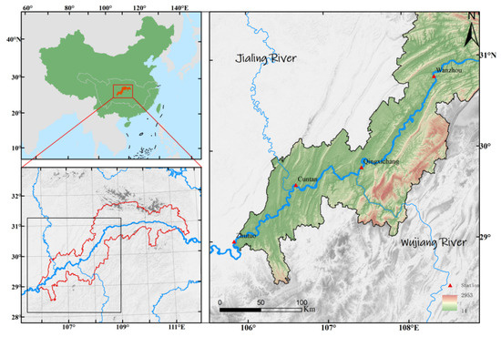
The Three Gorges Reservoir area is situated in western Hubei Province and central Chongqing Municipality, China (Figure 1). The regional climate is characterized by warm winters, early springs, hot summers, frequent autumn rainfall, high humidity, persistent cloud cover, and low wind speeds. This climatic regime not only intensifies watershed erosion and sediment yield but also severely limits the availability of high-quality optical remote sensing imagery, thereby complicating continuous monitoring of water and sediment processes. Four hydrological stations—Zhutuo (ZT), Cuntan (CT), Qingxichang (QXC), and Wanzhou (WZ)—are distributed sequentially from upstream to downstream, capturing the gradual transitions from the natural inflow reach, through the backwater fluctuation zone, to the middle section of the reservoir [24,25,26].

Figure 1. Study area and hydrological stations. The stations represent distinct hydrodynamic reaches along the mainstream: ZT (inflow control, upstream of backwater limit), CT (upper–middle fluctuating backwater zone), QXC (lower transitional backwater zone), and WZ (perennial backwater zone).

Although only four gauging stations are available, their spatial distribution captures the full longitudinal hydrodynamic gradient: ZT represents the natural inflow regime; CT and QXC span the fluctuating backwater zone where flow transitions from riverine to lacustrine conditions; and WZ characterizes the perennial backwater zone. Together with the 500 m interval spatial interpolation along the channel centerline and the JRC 30 m maximum water extent dataset for main channel extraction, this station network provides sufficient spatial coverage to depict the along-channel SSC trends across the reservoir.

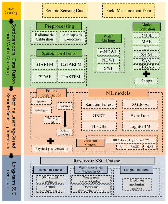
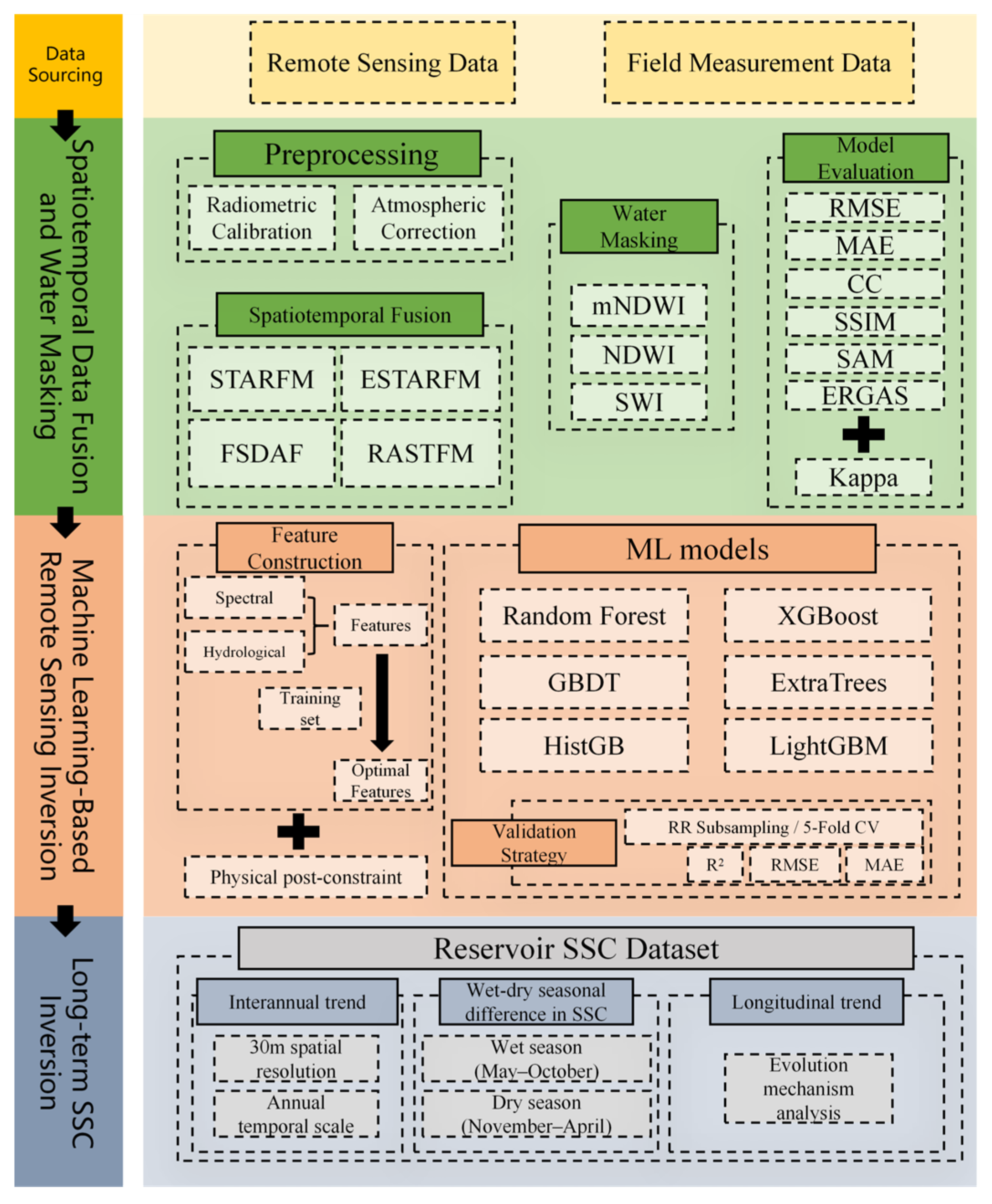
The overall research approach is illustrated (Figure 2), outlining the sequential workflow from multi-source data fusion and water mask extraction to feature engineering and machine learning-based SSC retrieval.

Figure 2. Research approach.

2.2. Data Sources and Technical Workflow

In situ SSC data for the same period were obtained from the Hydrological Yearbook of the Changjiang River Basin at four gauging stations: ZT, CT, QXC, and WZ. All SSC measurements were performed by the local hydrological authorities in accordance with the Chinese national standard GB/T 50159-2015 [27]. The standard gravimetric method was employed: water samples were filtered through pre-weighed 0.45 µm cellulose acetate membranes, oven-dried at 105 °C to constant weight, and the mass of sediment per unit volume of water was calculated. Duplicate analyses were conducted for each sample, and the mean value was recorded in the yearbook. The reported daily mean SSC values (kg/m³) were used for model calibration and validation.

Landsat (5/7/8) and the MODIS MOD09A1 product were selected as primary remote sensing data sources. Their complementary spatial and temporal resolutions were exploited for spatiotemporal fusion. Data processing was performed collaboratively on the Google Earth Engine platform and in local ENVI 5.6 software. To evaluate the regulatory effects of upstream cascade reservoir construction on sediment deposition within the reservoir area, Landsat Collection 2 Level-2 surface reflectance products and MODIS 8-day composite products spanning 2006–2020 were utilized. It is worth noting that the MOD09A1 product is composited from Terra satellite images acquired in the morning (local overpass time ~10:30), coinciding with the morning overpass of Landsat and the typical schedule of in situ suspended sediment sampling; this synchronization helps reduce diurnal differences in water reflectance and sediment concentration. For Landsat 7 ETM+SLC-off images, the local linear histogram matching method was applied to repair scan-line gaps. A dynamic cloud cover threshold of 20% was set, which was relaxed to 40% in years with insufficient clear-sky acquisitions. Visual inspection ensured adequate coverage of the main river channel. Images from three overlapping path/row tiles covering the study area were mosaicked, with priority given to acquisitions closest to the target date in overlapping regions (Table 1). From the initial 166 samples, 37 invalid ones were removed through visual interpretation and by filtering out outliers with reflectance values greater than 1, resulting in a final set of 129 valid Landsat raw sample images, including 41 for CT, 23 for WZ, 44 for ZT, and 21 for QXC.

Table 1. Specifications of the remote sensing data sources and spectral bands utilized.

Satellite Source	Band	Wavelength	Data Set	Resolution	Revisit Cycle	Range
Landsat5	Blue: SR_B1	0.45–0.52	C02/T1_L2	30	16	January 1984–May 2012
	Green: SR_B2	0.52–0.60
	Red: SR_B3	0.63–0.69
	NIR: SR_B4	0.76–0.90
	SWIR1: SR_B5	1.55–1.75
Landsat7	Blue: SR_B1	0.45–0.52	C02/T1_L2	30	16	April 1999–June 2025
	Green: SR_B2	0.52–0.60
	Red: SR_B3	0.63–0.69
	NIR: SR_B4	0.76–0.90
	SWIR1: SR_B5	1.55–1.75
Landsat8	Blue: SR_B2	0.45–0.51	C02/T1_L2	30	16	April 2013–Present
	Green: SR_B3	0.53–0.59
	Red: SR_B4	0.64–0.67
	NIR: SR_B5	0.85–0.88
	SWIR1: SR_B6	1.57–1.65
MODIS	Blue: Band3	0.459–0.479	MOD09A1	500	8	February 2000–Present
	Green: Band4	0.545–0.565
	Red: Band1	0.62–0.67
	NIR: Band2	0.841–0.876
	SWIR1: Band5	1.23–1.25

2.3. Spatiotemporal Fusion Algorithms

To ensure radiometric consistency between sensors, Landsat Collection 2 Level-2 surface reflectance (generated by LEDAPS/LaSRC): U.S. Geological Survey (USGS), Sioux Falls, SD, USA and MODIS daily surface reflectance product: NASA Level-1 and Atmosphere Archive and Distribution System (LAADS) Distributed Active Archive Center (DAAC), Greenbelt, MD, USA. were used. Both products have been atmospherically corrected using similar radiative transfer schemes and include quality assurance layers. MODIS bands (500 m) were resampled to the 30 m Landsat grid using nearest-neighbour resampling to match the spatial resolution. No further intersensor calibration was applied because the fusion algorithm internally resolves systematic spectral differences.

To identify the optimal fusion algorithm for subsequent matching with in situ measurements, the four candidates were compared using all available clear-sky MODIS–Landsat reference pairs (date difference < ±5 days). For each pair, the coarser MODIS image was fused to Landsat resolution, and the output was evaluated against the actual Landsat reflectance using the Root Mean Square Error (RMSE) and the coefficient of determination (R²) computed band by band. The algorithm that consistently delivered the lowest RMSE and highest R² across the visible and near-infrared bands was designated as the optimal fusion method. Its outputs were then used to construct the multi-temporal 30 m reflectance dataset for SSC retrieval, while the remaining algorithms were retained only for inter-comparison.

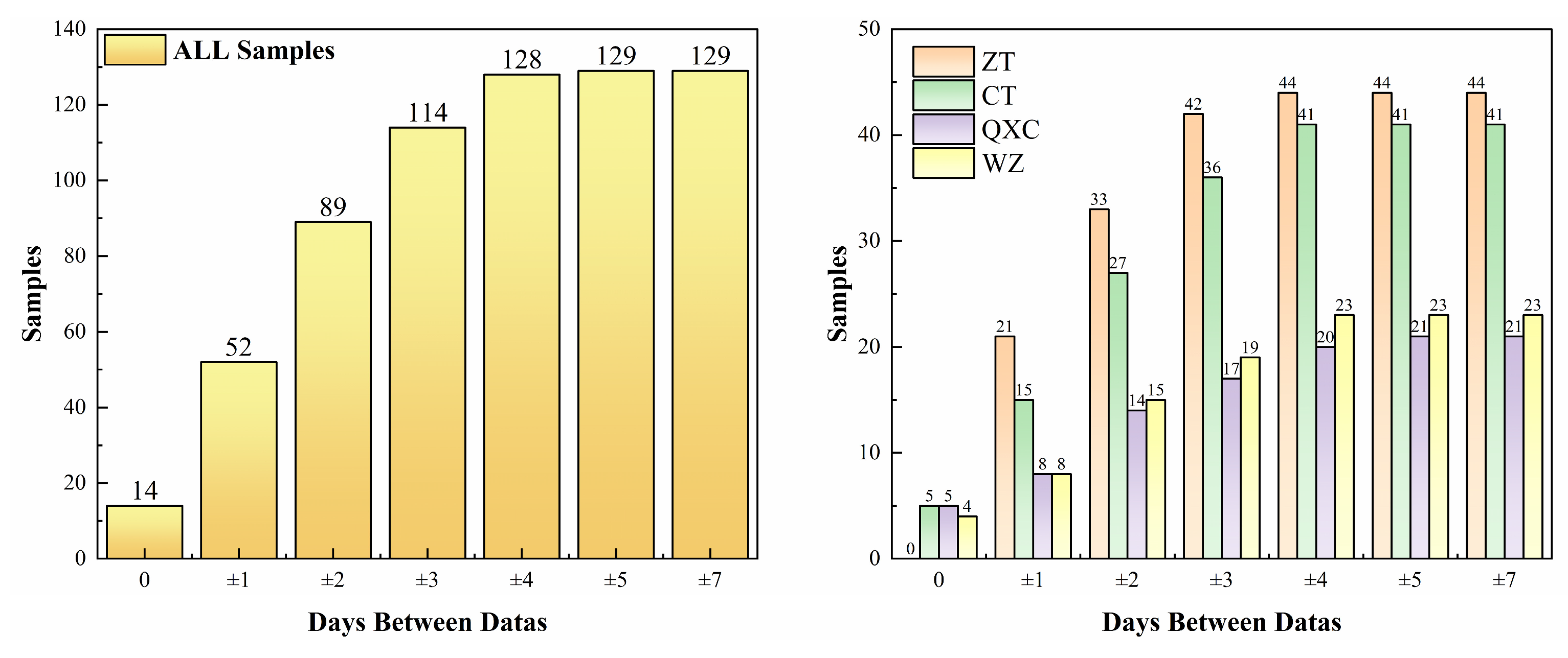
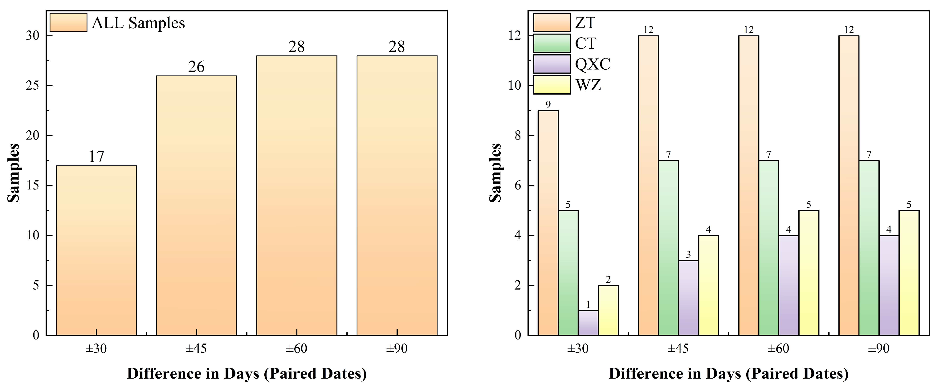
A temporal sensitivity analysis was conducted to determine the optimal matching scheme between satellite acquisitions and in situ SSC measurements at the four hydrological stations (ZT, CT, QXC, and WZ). All matching procedures used the Landsat overpass date as the reference date. For single-image matching, a single Landsat scene was paired with in situ data acquired within a given time window. The total number of valid pairs increased from 14 for exact-date matching (0-day) to 52 for ±1 day, 89 for ±2 days, 114 for ±3 days, and 128 for ±4 days, and plateaued at 129 pairs under both ±5-day and ±7-day windows (Figure 3). This indicates that a ±5-day tolerance is sufficient to maximize sample availability without introducing excessive temporal uncertainty. For dual-image matching, which builds upon the single-image matches, two adjacent Landsat scenes (one before and one after the in situ measurement date, both within a prescribed temporal window) were required. These dual-image pairs were designed to predict SSC for a window spanning 8 days before to 8 days after the Landsat reference date. Under this stricter constraint, far fewer pairs were obtained: from 17 at ±30 days to 26 at ±45 days and 28 at ±60 and ±90 days (Figure 4). Given the limited sample size of the dual-image scheme, the single-image matching with a ±5-day window was adopted as the operational criterion, yielding a final modeling dataset of 129 matched pairs [28].

Figure 3. Single pair matching base date (ZT, CT, QXC and WZ).

Figure 4. Couple matching base date (ZT, CT, QXC and WZ).

Because the reservoir is a channel-type impoundment with strong upstream flow regulation, daily SSC fluctuations are heavily damped under non-flood conditions. The day-to-day variability is generally smaller than the inherent retrieval uncertainty of the satellite data. This is corroborated by the sensitivity analysis, which shows that expanding the window from ± 3 to ± 5 days does not appreciably degrade validation accuracy. Therefore, the chosen window is hydrologically defensible.

Four spatiotemporal fusion algorithms—STARFM (Spatial and Temporal Adaptive Reflectance Fusion Model), ESTARFM (Enhanced STARFM) [29], FSDAF (Flexible Spatiotemporal Data Fusion) [30], and RASTFM—were applied to generate 30 m resolution fused reflectance imagery for target dates, using Landsat as the fine-resolution base and MODIS as the coarse-resolution input.

It should be noted that the fusion algorithms, particularly RASTFM, derive local regression coefficients from the reference MODIS–Landsat image pair, which inherently perform a band-wise radiometric normalization and effectively compensate for differences in sensor spectral response functions, view geometry, and atmospheric residuals. Hence, no separate cross-sensor spectral matching was applied prior to fusion.

The fused images were evaluated using the following six quantitative metrics: RMSE, Mean Absolute Error (MAE), Structural Similarity Index Measure (SSIM), Correlation Coefficient (CC), Spectral Angle Mapper (SAM), and Erreur Relative Globale Adimensionnelle de Synthèse (ERGAS):

$$\mathrm{R}\mathrm{M}\mathrm{S}\mathrm{E}=\sqrt{{\displaystyle \frac{1}{\mathrm{H}\mathrm{W}\mathrm{C}}}{\displaystyle \sum _{\mathrm{i}=1}^{\mathrm{H}}}{\displaystyle \sum _{\mathrm{j}=1}^{\mathrm{W}}}{\displaystyle \sum _{\mathrm{k}=1}^{\mathrm{C}}}{\left({\mathrm{R}}_{\mathrm{i}\mathrm{j}\mathrm{k}}-{\mathrm{F}}_{\mathrm{i}\mathrm{j}\mathrm{k}}\right)}^2}$$

(1)

$$\mathrm{M}\mathrm{A}\mathrm{E}={\displaystyle \frac{1}{\mathrm{H}\mathrm{W}\mathrm{C}}}{\displaystyle \sum _{\mathrm{i}=1}^{\mathrm{H}}}{\displaystyle \sum _{\mathrm{j}=1}^{\mathrm{W}}}{\displaystyle \sum _{\mathrm{k}=1}^{\mathrm{C}}}\left|{\mathrm{R}}_{\mathrm{i}\mathrm{j}\mathrm{k}}-{\mathrm{F}}_{\mathrm{i}\mathrm{j}\mathrm{k}}\right|$$

(2)

$$\mathrm{S}\mathrm{S}\mathrm{I}\mathrm{M}={\displaystyle \frac{(2{\mathsf{\mu }}_{\mathrm{R}}{\mathsf{\mu }}_{\mathrm{F}}+{\mathrm{c}}_1)(2{\mathsf{\sigma }}_{\mathrm{R}\mathrm{F}}+{\mathrm{c}}_2)}{({\mathsf{\mu }}_{\mathrm{R}}^2+{\mathsf{\mu }}_{\mathrm{F}}^2+{\mathrm{c}}_1)({\mathsf{\sigma }}_{\mathrm{R}}^2+{\mathsf{\sigma }}_{\mathrm{F}}^2+{\mathrm{c}}_2)}}$$

(3)

$$\mathrm{C}\mathrm{C}={\displaystyle \frac{{\sum }_{\mathrm{i}}{\sum }_{\mathrm{j}}({\mathrm{R}}_{\mathrm{i}\mathrm{j}}-\overline{\mathrm{R}})({\mathrm{F}}_{\mathrm{i}\mathrm{j}}-\overline{\mathrm{F}})}{\sqrt{{\sum }_{\mathrm{i}}{\sum }_{\mathrm{j}}{({\mathrm{R}}_{\mathrm{i}\mathrm{j}}-\overline{\mathrm{R}})}^2}\sqrt{\sum _{\mathrm{i}}{\sum }_{\mathrm{j}}{({\mathrm{F}}_{\mathrm{i}\mathrm{j}}-\overline{\mathrm{F}})}^2}}}$$

(4)

$$\mathrm{S}\mathrm{A}\mathrm{M}={\cos }^{-1}({\displaystyle \frac{{\sum }_{\mathrm{k}=1}^{\mathrm{C}}{\mathrm{R}}_{\mathrm{i}\mathrm{j}\mathrm{k}}{\mathrm{F}}_{\mathrm{i}\mathrm{j}\mathrm{k}}}{\sqrt{{\sum }_{\mathrm{k}=1}^{\mathrm{C}}{\mathrm{R}}_{\mathrm{i}\mathrm{j}\mathrm{k}}^2}\sqrt{{\sum }_{\mathrm{k}=1}^{\mathrm{C}}{\mathrm{F}}_{\mathrm{i}\mathrm{j}\mathrm{k}}^2}}})$$

(5)

$$\mathrm{E}\mathrm{R}\mathrm{G}\mathrm{A}\mathrm{S}=100·{\displaystyle \frac{\mathrm{l}}{\mathrm{h}}}\sqrt{{\displaystyle \frac{1}{\mathrm{C}}}{\displaystyle \sum _{\mathrm{k}=1}^{\mathrm{C}}}{\left({\displaystyle \frac{\mathrm{R}\mathrm{M}\mathrm{S}{\mathrm{E}}_{\mathrm{k}}}{{\mathsf{\mu }}_{\mathrm{k}}}}\right)}^2}$$

(6)

These six indices respectively assess pixel-level error magnitude, average bias, structural similarity, correlation, spectral distortion, and resolution-normalized global error. Therefore, they provide a comprehensive evaluation of radiometric accuracy, spatial detail preservation, perceptual quality, spectral fidelity, and overall fused image quality.

2.4. Water Mask Extraction and Optimization

The accuracy of water body extraction directly influences the purity of sample pixels used in subsequent SSC retrieval. Based on the optimally fused imagery, three widely used water indices were computed and compared.

The NDWI is defined as:

$$\mathrm{N}\mathrm{D}\mathrm{W}\mathrm{I}={\displaystyle \frac{\mathrm{G}\mathrm{r}\mathrm{e}\mathrm{e}\mathrm{n}-\mathrm{N}\mathrm{I}\mathrm{R}}{\mathrm{G}\mathrm{r}\mathrm{e}\mathrm{e}\mathrm{n}+\mathrm{N}\mathrm{I}\mathrm{R}}}$$

(7)

The MNDWI is defined as:

$$\mathrm{M}\mathrm{N}\mathrm{D}\mathrm{W}\mathrm{I}={\displaystyle \frac{\mathrm{G}\mathrm{r}\mathrm{e}\mathrm{e}\mathrm{n}-\mathrm{S}\mathrm{W}\mathrm{I}\mathrm{R}1}{\mathrm{G}\mathrm{r}\mathrm{e}\mathrm{e}\mathrm{n}+\mathrm{S}\mathrm{W}\mathrm{I}\mathrm{R}1}}$$

(8)

Although the water-leaving reflectance of clean water in the SWIR1 band is close to zero, the study area is characterized by persistently high-SSC, under which the SWIR1 reflectance is significantly higher than zero and can respond to variations in suspended sediment. Furthermore, incorporating SWIR1 into band-ratio indices helps to suppress residual atmospheric correction errors and surface reflection artifacts, thereby improving the robustness of the retrieval model. The feature importance ranking derived from our model also confirms that SWIR-related features contribute meaningfully to the predictions.

The SWI is defined as:

$$\mathrm{S}\mathrm{W}\mathrm{I}=\mathrm{B}\mathrm{l}\mathrm{u}\mathrm{e}+\mathrm{G}\mathrm{r}\mathrm{e}\mathrm{e}\mathrm{n}-\mathrm{N}\mathrm{I}\mathrm{R}$$

(9)

Threshold sensitivity analysis was conducted to determine the optimal segmentation threshold for each water index at each hydrological station. Thresholds were iterated from −0.5 to 0.8 with a step size of 0.01. For each threshold, the resulting water classification was compared against the Joint Research Centre (JRC) Global Surface Water 30 m maximum water extent reference dataset, and the Kappa coefficient was computed. The threshold maximizing the Kappa coefficient was selected as the optimal water–land separation value. The Kappa coefficient is calculated as:

$$\mathrm{O}\mathrm{A}={\displaystyle \frac{\mathrm{T}\mathrm{P}+\mathrm{T}\mathrm{N}}{\mathrm{T}\mathrm{P}+\mathrm{F}\mathrm{P}+\mathrm{T}\mathrm{N}+\mathrm{F}\mathrm{N}}}$$

(10)

$${\mathrm{F}}_1={\displaystyle \frac{2\mathrm{TP}}{2\mathrm{TP}+\mathrm{FN}+\mathrm{FN}}}$$

(11)

where TP, FP, FN, and TN denote true positives, false positives, false negatives, and true negatives, respectively.

$$\mathsf{\kappa }={\displaystyle \frac{{\mathrm{p}}_0-{\mathrm{p}}_{\mathrm{e}}}{1-{\mathrm{p}}_{\mathrm{e}}}}$$

(12)

where ${\mathrm{p}}_0$ is the overall classification accuracy, and ${\mathrm{p}}_{\mathrm{e}}$ is the expected agreement by chance.

2.5. Machine Learning Retrieval Models

To balance station representativeness and mixed-pixel effects while enhancing model accuracy, optimal fused images and original Landsat images were matched with in situ SSC measurements on the same dates. A 5 km buffer zone was delineated within the optimal water mask, and samples with anomalous remote sensing reflectance were removed, yielding the final “hydrology–remote sensing” matched dataset.

Owing to persistent cloud cover and the stringent requirement for temporally coincident in situ measurements, the final matched dataset remains relatively small. This limits the reliable capture of extremely high-SSC events, particularly at stations with few available measurements.

A total of 227 candidate features representing spectral, hydrological, and their interactions were constructed from the fused Landsat reflectance and synchronous river discharge (Q), with the in situ SSC strictly reserved as the response variable. The features fell into four groups:

(1) Normalized band reflectance–each of the five reflective bands (Blue, Green, Red, NIR, SWIR1) was divided by the sum of those five bands, yielding five normalized reflectance values that suppress illumination variations and residual atmospheric effects; (2) Band arithmetic combinations—all pairwise ratios (e.g., Green/Red), differences, and products were computed, along with three-band combinations of the forms $(\mathrm{R}\mathrm{i}-\mathrm{R}\mathrm{j})/(\mathrm{R}\mathrm{i}+\mathrm{R}\mathrm{j})$ and $(\mathrm{R}\mathrm{i}-\mathrm{R}\mathrm{j})/(\mathrm{R}\mathrm{k}-\mathrm{R}\mathrm{j})$. These arithmetic features follow well-established semi-analytical and empirical approaches that enhance the signal-to-noise ratio of suspended particle backscattering relative to pure water and dissolved organic matter; (3) Established water-related indices—NDVI, NDWI, MNDWI, SWI and so on, which are sensitive to water-leaving radiance, turbidity, and aquatic vegetation in highly turbid inland waters; (4) Flow–spectral interaction features—the concurrent discharge Q was directly multiplied with each Five band and each band ratio (e.g., Q × (Green/Red), Q × NIR). Discharge is a primary driver of sediment resuspension, advection, and dilution in the Three Gorges Reservoir; coupling it with spectral quantities creates features that capture the non-linear joint influence of hydrodynamics and optically active constituents.

To avoid overfitting, the curse of dimensionality, and data leakage, feature selection was performed dynamically using Pearson correlation coefficients computed exclusively on the training set, retaining the 20 most explanatory features. Although Pearson correlation captures only linear dependencies, the feature set already encodes nonlinear relationships through the flow–spectral interaction terms such as Q × band, which explicitly couple discharge dynamics with optical signals. SHAP analysis further confirms that these top-ranked features remain consistently dominant, demonstrating that the Pearson-based screening did not omit critical nonlinear predictors. Hence, Pearson correlation can justifiably serve as an interpretable baseline for variable importance analysis in this study.

Six representative tree-based ensemble models were selected for evaluation: Random Forest (RF), ExtraTrees, Gradient Boosting Decision Tree (GBDT), HistGB, Extreme Gradient Boosting (XGBoost), and Light Gradient Boosting Machine (LightGBM). These models offer advantages in handling nonlinear relationships, noise robustness, and automatic feature interaction.

To rigorously assess model performance, the dataset was partitioned into training and testing subsets at an 8:2 ratio. For each hydrological station (ZT, CT, QXC, and WZ), a repeated random subsampling validation procedure was executed over 50 iterations, supplemented by a 5-fold cross-validation strategy as a complementary evaluation. Model accuracy was quantified using the following statistical metrics: the R², which is equivalent to the Nash-Sutcliffe Efficiency (NSE), along with the RMSE and MAPE.

$${\mathrm{R}}^2=\mathrm{N}\mathrm{S}\mathrm{E}=1-{\displaystyle \frac{{\sum }_{\mathrm{i}=1}^{\mathrm{n}}{({\mathrm{y}}_{\mathrm{i}}-\widehat{{\mathrm{y}}_{\mathrm{i}}})}^2}{{\sum }_{\mathrm{i}=1}^{\mathrm{n}}{({\mathrm{y}}_{\mathrm{i}}-\overline{\mathrm{y}})}^2}}$$

(13)

$$\mathrm{R}\mathrm{M}\mathrm{S}\mathrm{E}=\sqrt{{\displaystyle \sum _{\mathrm{i}=1}^{\mathrm{n}}}{\displaystyle \frac{{({\widehat{\mathrm{y}}}_{\mathrm{i}}-{\mathrm{y}}_{\mathrm{i}})}^2}{\mathrm{n}}}}$$

(14)

$$\mathrm{M}\mathrm{A}\mathrm{P}\mathrm{E}=100\%\times {\displaystyle \frac{1}{\mathrm{n}}}{\displaystyle \sum _{\mathrm{i}=1}^{\mathrm{n}}}\left|{\displaystyle \frac{{\widehat{\mathrm{y}}}_{\mathrm{i}}-{\mathrm{y}}_{\mathrm{i}}}{{\mathrm{y}}_{\mathrm{i}}}}\right|$$

(15)

where ${\mathrm{y}}_{\mathrm{i}}$ is the measured SSC (kg/m³) of the $\mathrm{i}$-th sample, $\widehat{{\mathrm{y}}_{\mathrm{i}}}$ is the corresponding predicted concentration, $\overline{\mathrm{y}}$ is the mean of all measured concentrations, and $\mathrm{n}$ is the total number of samples.

These three indices assess model explanatory power, absolute deviation, and relative deviation, respectively. Samples with measured SSC values below 10⁻³ kg/m³ were excluded from the MAPE calculation to avoid division-by-zero instability. Given that MAPE can be disproportionately inflated at stations with low SSC values and a high proportion of low-concentration samples, model comparisons were primarily based on R² and RMSE.

Purely data-driven models may produce predictions that violate physical plausibility under extreme water–sediment conditions. A soft-constraint post-processing strategy incorporating in situ suspended sediment measurements was therefore introduced. To avoid excessively restrictive constraints, a sensitivity analysis was performed with thresholds ranging from 0.1 to 0.8 at 0.05 increments. The physical constraint post-processing formula is:

$$\overline{{\mathrm{y}}_{\mathrm{i}}}=\left\{\begin{array}{c}\widehat{y_i}, \widehat{y_i}\le \widetilde{y_i}\\ \widehat{y_i}+\alpha (\widetilde{y_i}-\widehat{y_i}), \widehat{y_i}>\widetilde{y_i}\end{array}\right.$$

(16)

where $\overline{{\mathrm{y}}_{\mathrm{i}}}$ is the corrected value, $\widehat{y_i}$ is the original machine learning model prediction, $\widetilde{y_i}$ is the measured SSC of the same day if available, otherwise the historical maximum SSC at that station during the modeling period (2006–2020), and $\alpha$ is a relaxation coefficient.

3. Results

3.1. Performance Comparison of Spatiotemporal Fusion Algorithms

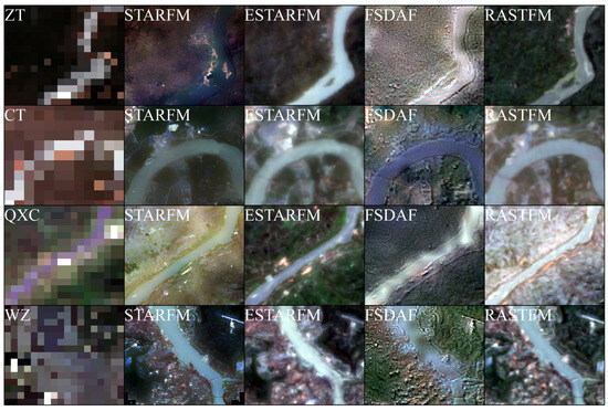
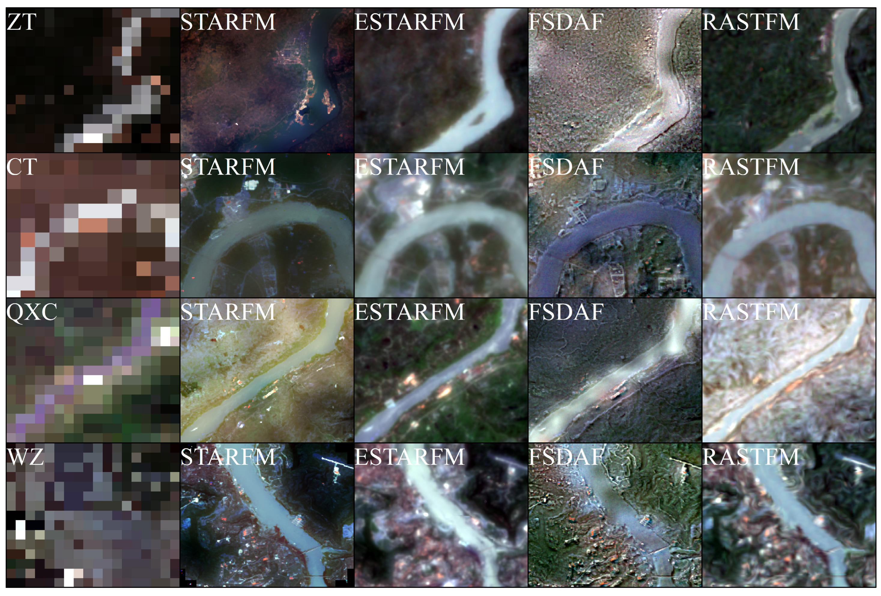
The quantitative evaluation results of the four spatiotemporal fusion algorithms at the four hydrological stations are presented (Table 2). Across all stations, RASTFM achieved the lowest RMSE and MAE and the highest CC, with SAM also indicating minimal spectral distortion. STARFM ranked second and yielded the highest SSIM at the ZT, QXC, and WZ stations. In contrast, FSDAF consistently exhibited the largest SAM (0.750–0.880) and the highest ERGAS (5.82–9.41) across all stations [31]. Notably, FSDAF maintained a relatively high CC at the CT station (0.938), suggesting that despite systematic radiometric deviation, it partially preserved the relative spatial variation patterns of surface reflectance.

Table 2. Performance comparison of four spatiotemporal fusion algorithms (STARFM, ESTARFM, FSDAF, and RASTFM) across the four hydrological stations.

Station	Fusion Method	RMSE	MAE	SSIM	CC	SAM	ERGAS
ZT	STARFM	0.032	0.017	0.797	0.879	0.536	2.12
	ESTARFM	0.051	0.024	0.615	0.772	0.557	2.82
	FSDAF	0.106	0.086	0.461	0.786	0.859	9.41
	RASTFM	0.023	0.011	0.738	0.928	0.410	1.44
CT	STARFM	0.050	0.025	0.618	0.769	0.587	3.19
	ESTARFM	0.046	0.026	0.772	0.793	0.669	2.85
	FSDAF	0.073	0.056	0.489	0.937	0.750	5.82
	RASTFM	0.026	0.010	0.800	0.938	0.452	1.78
QXC	STARFM	0.035	0.019	0.777	0.837	0.543	2.34
	ESTARFM	0.047	0.023	0.621	0.759	0.563	2.76
	FSDAF	0.197	0.165	0.462	0.788	0.880	8.63
	RASTFM	0.023	0.010	0.758	0.935	0.407	1.34
WZ	STARFM	0.036	0.019	0.831	0.848	0.543	2.39
	ESTARFM	0.053	0.027	0.684	0.766	0.572	2.94
	FSDAF	0.077	0.058	0.485	0.720	0.774	7.24
	RASTFM	0.026	0.012	0.789	0.925	0.419	1.58

Visual comparison of the four algorithms reveals marked divergence in spectral fidelity and spatial detail preservation (Figure 5). As illustrated, the reconstruction of water boundary sharpness and spectral consistency within shadowed areas varied substantially among the fusion strategies [32].

Figure 5. Performance comparison of spatiotemporal fusion algorithms.

3.2. Accuracy Analysis of Water Index Extraction

Threshold sensitivity analysis and accuracy assessment results are summarized (Table 3). MNDWI performed best at the ZT, CT, and QXC stations—reaches significantly affected by terrain shadowing and urban infrastructure–achieving overall accuracies, F1 scores, and Kappa coefficients of 0.96/0.71/0.69, 0.96/0.72/0.70, and 0.98/0.83/0.82. At the WZ station, NDWI yielded the optimal performance, with an accuracy of 0.97, an F1 score of 0.87, and a Kappa coefficient of 0.86. SWI exhibited unstable performance across stations, with optimal thresholds fluctuating substantially between 0.04 and 0.08 and consistently yielding the lowest F1 scores and Kappa coefficients. Unlike MNDWI, SWI does not incorporate the SWIR band, where water reflectance is nearly zero and shadow discrimination is most robust. Moreover, as an arithmetic combination (Blue + Green − NIR) rather than a band ratio, SWI is highly sensitive to absolute reflectance variations driven by spatially and temporally varying SSC, which simultaneously elevate both the (Blue + Green) and NIR terms in unpredictable proportions. This dual sensitivity causes the optimal water–land separation threshold to vary erratically from station to station. Based on the Kappa-maximization criterion, MNDWI with thresholds of 0.23, 0.13, and 0.18 was applied for water masking at ZT, CT, and QXC, respectively, while NDWI with a threshold of 0.00 was used at WZ. This outcome is consistent with the open-channel and relatively shadow-free setting of WZ, where the simple green–NIR contrast is sufficient for accurate water–land delineation without the need for SWIR-based shadow suppression. The JRC 30 m maximum water extent dataset was additionally used to mask out isolated non-river water pixels and preserve the main channel.

Table 3. Optimal thresholds and accuracy assessment of water body extraction using NDWI, MNDWI and SWI at the four hydrological stations.

Station	Water Index	Threshold	Overall Accuracy	F1	Kappa Coefficient
ZT	NDWI	Water > 0.02	0.95	0.67	0.65
	MNDWI	Water > 0.23	0.96	0.71	0.69
	SWI	Water > 0.04	0.93	0.68	0.64
CT	NDWI	Water > −0.11	0.95	0.65	0.63
	MNDWI	Water > 0.13	0.96	0.72	0.70
	SWI	Water > 0.08	0.94	0.57	0.53
QXC	NDWI	Water > −0.09	0.98	0.80	0.79
	MNDWI	Water > 0.18	0.98	0.83	0.82
	SWI	Water > 0.04	0.97	0.78	0.76
WZ	NDWI	Water > 0.00	0.97	0.87	0.86
	MNDWI	Water > 0.18	0.97	0.85	0.84
	SWI	Water > 0.06	0.94	0.73	0.70

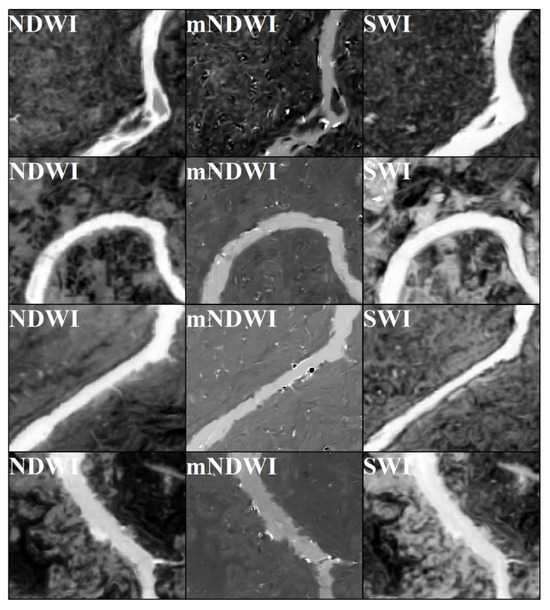
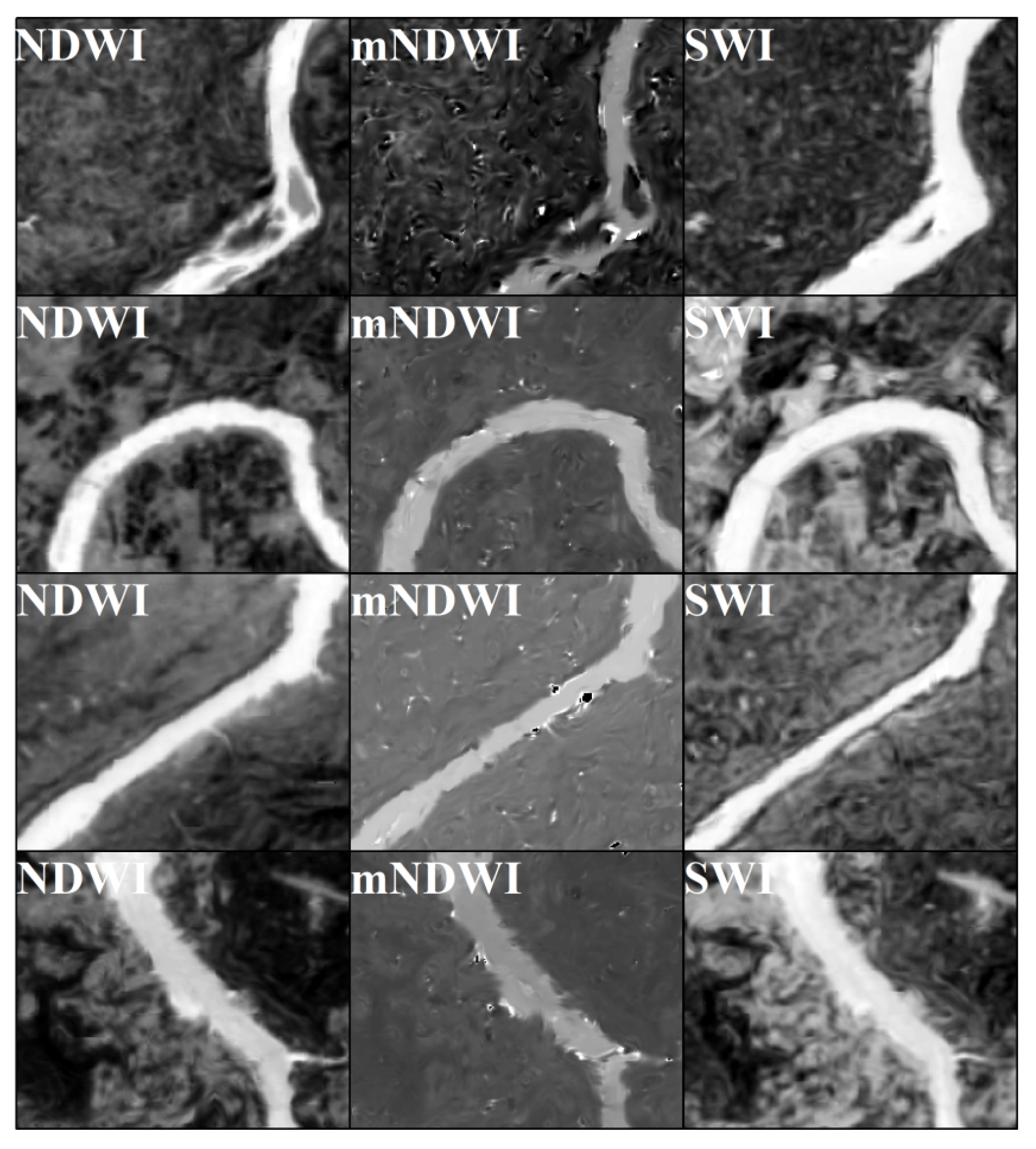
Based on the RASTFM fused imagery, water masks were generated by applying the station-specific optimal indices and thresholds on a per-pixel basis (Figure 6).

Figure 6. Water Mask extraction results at the four hydrological stations.

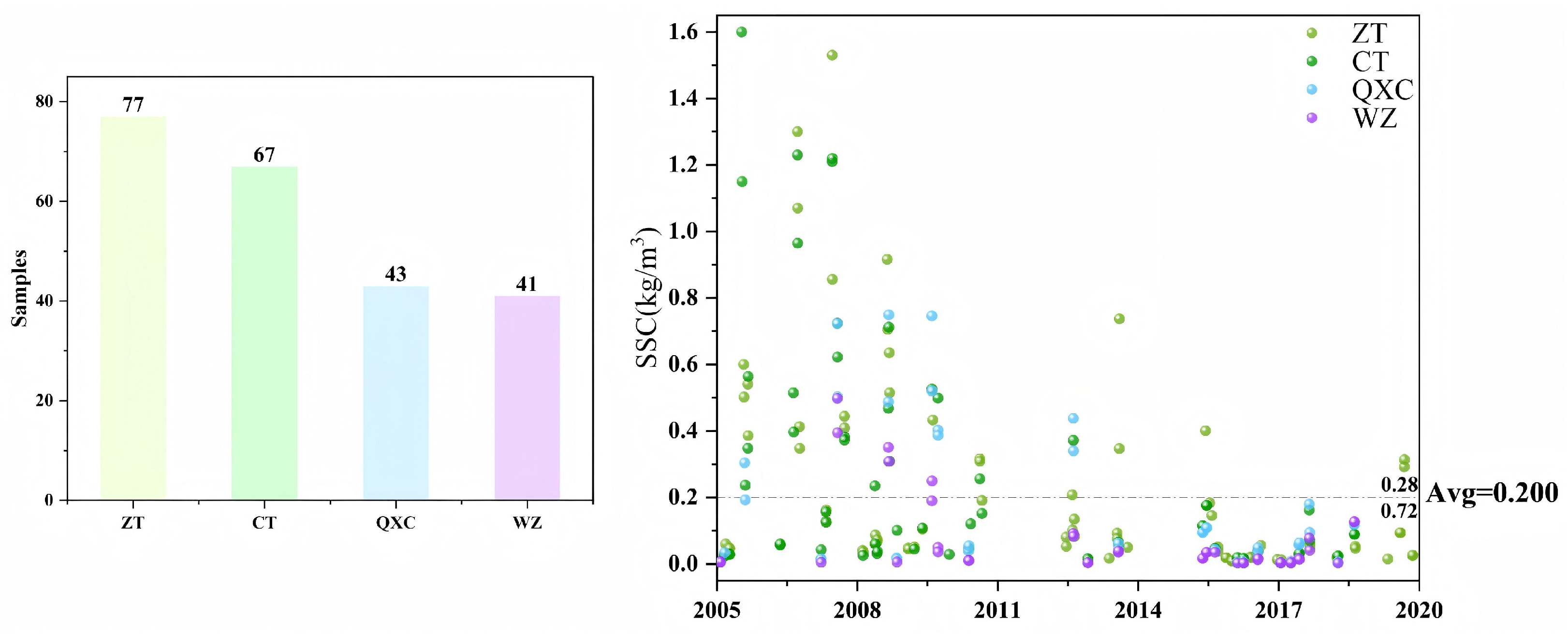
Following spatiotemporal fusion, water mask extraction, and outlier removal, a total of 228 valid image scenes were obtained: 77 at ZT, 67 at CT, 43 at QXC, and 41 at WZ. Compared with the 129 Landsat-only scenes available across the four stations, this represents an increase of 99 high-quality effective images—a 77% enhancement in usable high-precision imagery.

3.3. Accuracy Comparison of Machine Learning Retrieval Models

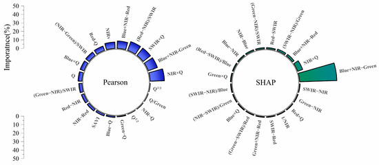
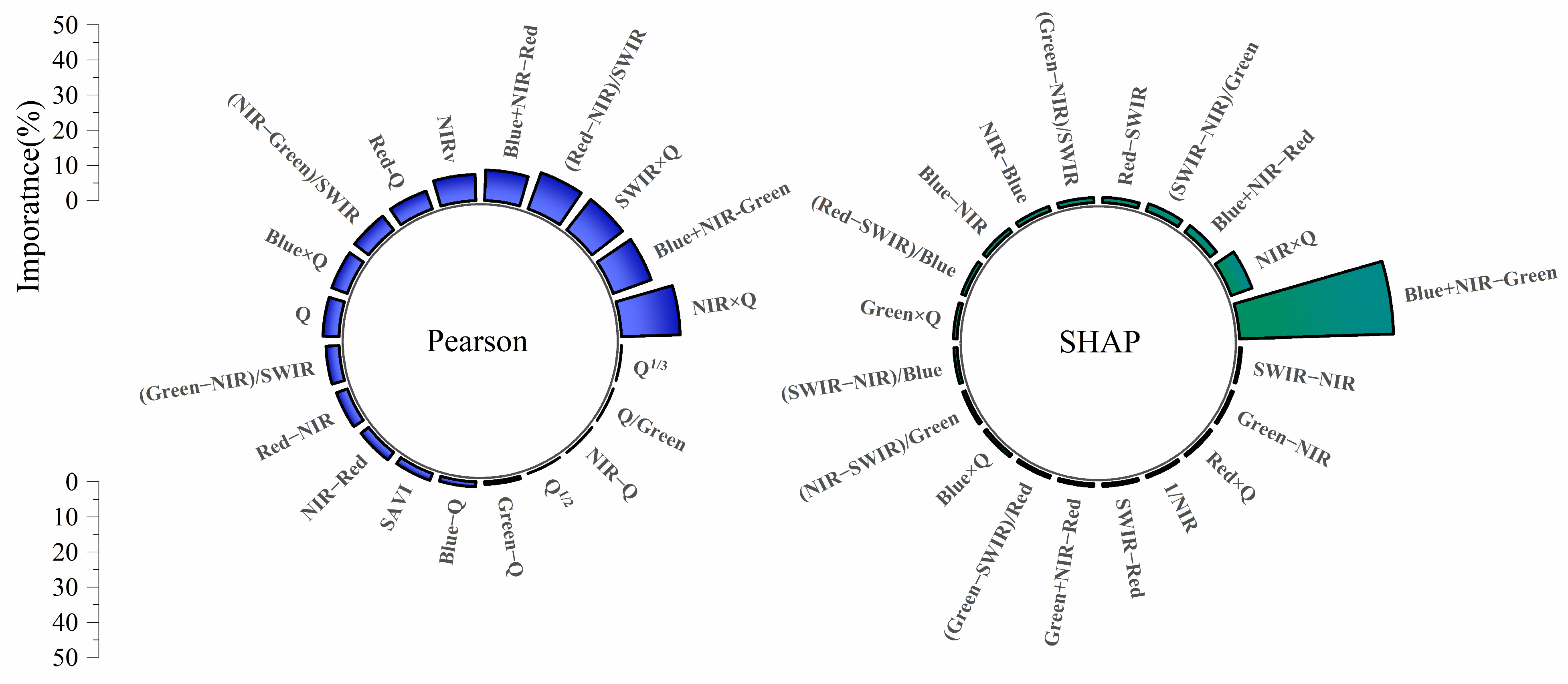
The top-20 feature importance ranking (Figure 7). shows that both Pearson correlation and SHAP consistently identify NIR × Q and Blue + NIR − Green as the most important features, with their importance substantially surpassing that of all other variables. Pearson correlation yields the highest coefficient for NIR × Q, followed by Blue + NIR − Green and SWIR × Q, capturing strong linear relationships with computational simplicity and high interpretability, while SHAP ranks Blue + NIR − Green first and NIR × Q second, thereby revealing their nonlinear coupling effects with SSC. This strong agreement confirms that these discharge–spectral joint features carry not only robust linear signatures readily detected by Pearson but also complex nonlinear effects. Meanwhile, Blue + NIR − Red also demonstrates a notable level of importance, whereas simple band differences rank low in both rankings.

Figure 7. Pearson and based RF SHAP Feature Importance.

NIR reflectance serves as a proxy for SSC, while discharge Q captures the hydraulic driving force; their product thus acts as a sediment-transport proxy, amplifies flood-event signals, and resolves ambiguities in scenarios where high Q coincides with low SSC or vice versa. Blue + NIR − Green, a spectral index derived from SHAP analysis, exploits the strong scattering of suspended sediments in the blue and NIR bands together with the relative clarity of the green band, offering a complementary optical discriminator. Under the small-sample, skewed-distribution conditions of this study, both features proved exceptionally robust, underpinning their top importance.

The ZT, CT, and WZ stations were insensitive to threshold variations, and QXC exhibited only negligible sensitivity.

Hyperparameters for each model were determined through a preliminary grid search combined with empirical tuning, aiming to balance fitting capacity and generalization performance. The final hyperparameter settings are listed (Table 4).

Table 4. Hyperparameter settings of machine learning models.

Model	Hyperparameter Settings
Random Forest	n_estimators = 200, max_depth = 8, min_samples_split = 5, min_samples_leaf = 2
ExtraTrees	n_estimators = 200, max_depth = 8, min_samples_split = 5, min_samples_leaf = 2
Gradient Boosting	n_estimators = 200, learning_rate = 0.05, max_depth = 4, subsample = 0.8, min_samples_split = 5
HistGB	max_iter = 200, learning_rate = 0.05, max_depth = 4, min_samples_leaf = 10
XGBoost	n_estimators = 200, learning_rate = 0.05, max_depth = 4, subsample = 0.8, colsample_bytree = 0.8, reg_alpha = 0.1, reg_lambda = 1.0
LightGBM	n_estimators = 200, learning_rate = 0.05, num_leaves = 31, max_depth = 4, subsample = 0.8, reg_alpha = 0.1, reg_lambda = 1.0

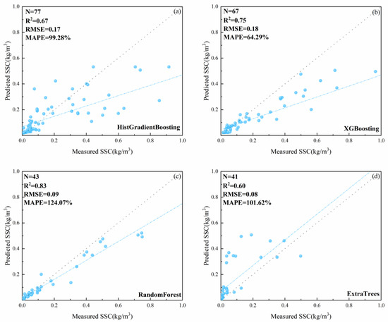
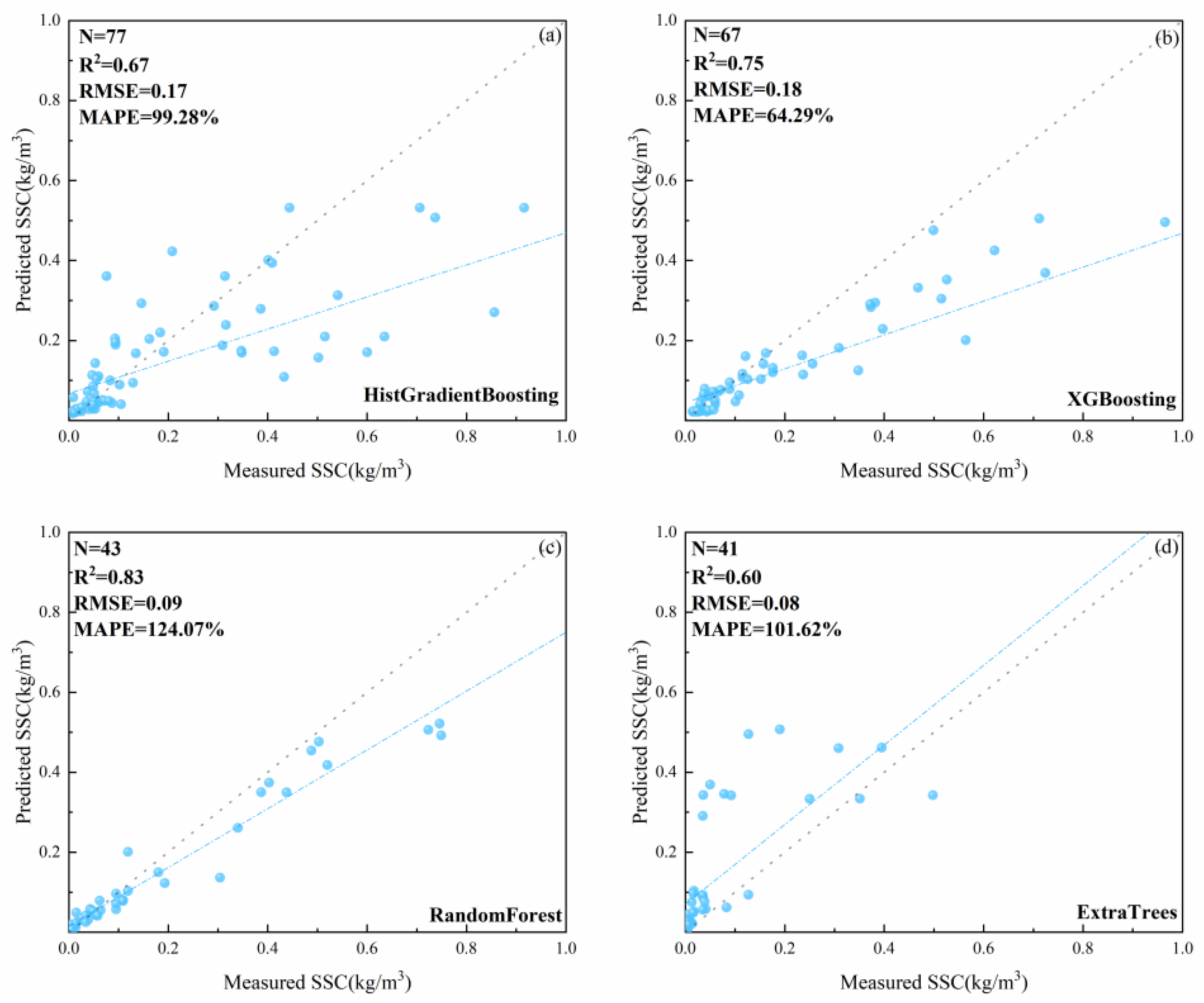
The results of repeated random subsampling validation at the four stations are presented (Table 5). Model performance exhibited pronounced inter-station and inter-model variability. At ZT, HistGB performed best (R² = 0.67 ± 0.11); at CT, XGBoost achieved the highest R² (R² = 0.75 ± 0.12); at QXC, RF attained an R² of 0.83 ± 0.06 with an RMSE as low as 0.09; and at WZ, ExtraTrees was relatively optimal (R² = 0.60 ± 0.17). ExtraTrees, HistGB, and XGBoost demonstrated relatively high predictive accuracy and stability across most stations [33]. In contrast, LightGBM performed poorly at all stations; at QXC, its R² was merely 0.14 ± 0.04, and MAPE reached 412.80%. At the QXC station, the limited number of field samples—coupled with the fact that the majority fall below the mean while high-concentration cases are extremely rare—makes the model particularly vulnerable to single-point perturbation. The inflated MAPE (412%) thus reflects a structural data deficiency at both the low and high ends of the concentration distribution, rather than inadequate hyperparameter optimization. Since MAPE is significantly amplified in the low-value region, R² and RMSE are used as the primary references, while MAPE is only used for inter-model comparison.

Table 5. Performance comparison of six machine learning models under repeated random subsampling validation at the four hydrological stations.

Station	Models	Repeated Random Subsampling			Station	Models	Repeated Random Subsampling
		R2	RMSE (kg/m3)	MAPE (%)			R2	RMSE (kg/m3)	MAPE (%)
ZT	ExtraTrees	0.63 ± 0.09	0.18	87.59	QXC	ExtraTrees	0.79 ± 0.07	0.10	130.53
	GBDT	0.64 ± 0.11	0.17	88.07		GBDT	0.80 ± 0.07	0.10	111.65
	HistGB	0.67 ± 0.11	0.17	99.28		HistGB	0.83 ± 0.07	0.09	95.53
	LightGBM	0.65 ± 0.11	0.17	85.45		LightGBM	0.14 ± 0.04	0.18	412.80
	RF	0.66 ± 0.07	0.16	90.96		RF	0.83 ± 0.06	0.09	124.07
	XGBoost	0.63 ± 0.11	0.18	85.98		XGBoost	0.79 ± 0.06	0.10	129.31
CT	ExtraTrees	0.70 ± 0.11	0.20	59.71	WZ	ExtraTrees	0.60 ± 0.17	0.08	101.62
	GBDT	0.69 ± 0.13	0.20	66.56		GBDT	0.53 ± 0.18	0.08	132.69
	HistGB	0.71 ± 0.10	0.19	76.78		HistGB	0.59 ± 0.12	0.07	183.94
	LightGBM	0.66 ± 0.09	0.21	97.17		LightGBM	0.13 ± 0.06	0.08	390.81
	RF	0.71 ± 0.10	0.20	68.14		RF	0.53 ± 0.16	0.08	130.63
	XGBoost	0.75 ± 0.12	0.18	64.29		XGBoost	0.59 ± 0.15	0.08	157.03

Scatter density plots comparing predicted versus measured SSC for the optimal model at each station are shown (Figure 8). The ZT and CT models exhibited robust performance; QXC demonstrated the highest consistency; and WZ, owing to lower absolute SSC values, showed slightly increased dispersion.

Figure 8. Scatter density plots of predicted versus measured SSC for the optimal machine learning models at the four hydrological stations. (a) ZT; (b) CT; (c) QXC; (d) WZ.

Five-fold cross-validation results are presented. Overall model stability under this validation scheme was moderate (Table 6). The standard deviation of R² for the optimal model at each station ranged from 0.07 to 0.34. The RF model at QXC exhibited the highest stability (R² = 0.84 ± 0.07), whereas the HistGB model at ZT showed relatively lower stability (R² = 0.54 ± 0.29). Although HistGB and RF achieved comparable mean R² at QXC, RF exhibited lower variance in repeated subsampling and superior stability in 5-fold cross-validation; hence, it was selected as the operational model for QXC.

Table 6. Performance of the optimal machine learning models at each station evaluated via 5-fold cross-validation.

Station	Models	R2	RMSE (kg/m3)	MAPE (%)
ZT	HistGB	0.54 ± 0.29	0.175 ± 0.036	92.8 ± 27.4
CT	XGBoost	0.65 ± 0.20	0.210 ± 0.085	64.7 ± 19.3
QXC	RF	0.84 ± 0.07	0.082 ± 0.025	116.5 ± 109.9
WZ	ExtraTrees	0.70 ± 0.34	0.064 ± 0.057	67.2 ± 30.0

3.4. Spatiotemporal SSC Retrieval Results

Based on the selected RASTFM fused imagery, the center point of each pixel was projected onto the river centerline to determine its spatial position. Pixel values were averaged at 500 m intervals along the river course to generate 30 m resolution SSC distribution maps for the ZT to WZ reach of the Three Gorges Reservoir for each year from 2006 to 2020, as well as for the wet season (May–October) and dry season (November–April) separately.

$$\mathrm{S}\mathrm{S}\mathrm{C}={\mathrm{w}}_{\mathrm{u}\mathrm{p}}{\mathrm{S}\mathrm{S}\mathrm{C}}_{\mathrm{u}\mathrm{p}}+{\mathrm{w}}_{\mathrm{d}\mathrm{o}\mathrm{w}\mathrm{n}}{\mathrm{S}\mathrm{S}\mathrm{C}}_{\mathrm{d}\mathrm{o}\mathrm{w}\mathrm{n}}$$

(17)

where the weights are inversely proportional to the respective distances: ${\mathrm{w}}_{\mathrm{u}\mathrm{p}}={\displaystyle \frac{{\mathrm{d}}_{\mathrm{d}\mathrm{o}\mathrm{w}\mathrm{n}}}{{\mathrm{d}}_{\mathrm{u}\mathrm{p}}+{\mathrm{d}}_{\mathrm{d}\mathrm{o}\mathrm{w}\mathrm{n}}}}$, ${\mathrm{w}}_{\mathrm{d}\mathrm{o}\mathrm{w}\mathrm{n}}={\displaystyle \frac{{\mathrm{d}}_{\mathrm{u}\mathrm{p}}}{{\mathrm{d}}_{\mathrm{u}\mathrm{p}}+{\mathrm{d}}_{\mathrm{d}\mathrm{o}\mathrm{w}\mathrm{n}}}}$, ${\mathrm{d}}_{\mathrm{u}\mathrm{p}}$ is the distance from the target point to the upstream hydrological station, and ${\mathrm{d}}_{\mathrm{d}\mathrm{o}\mathrm{w}\mathrm{n}}$ is the distance from the target point to the downstream hydrological station.

3.4.1. Interannual Along-Channel SSC Variation Characteristics

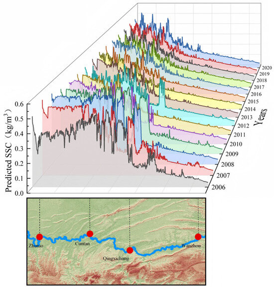
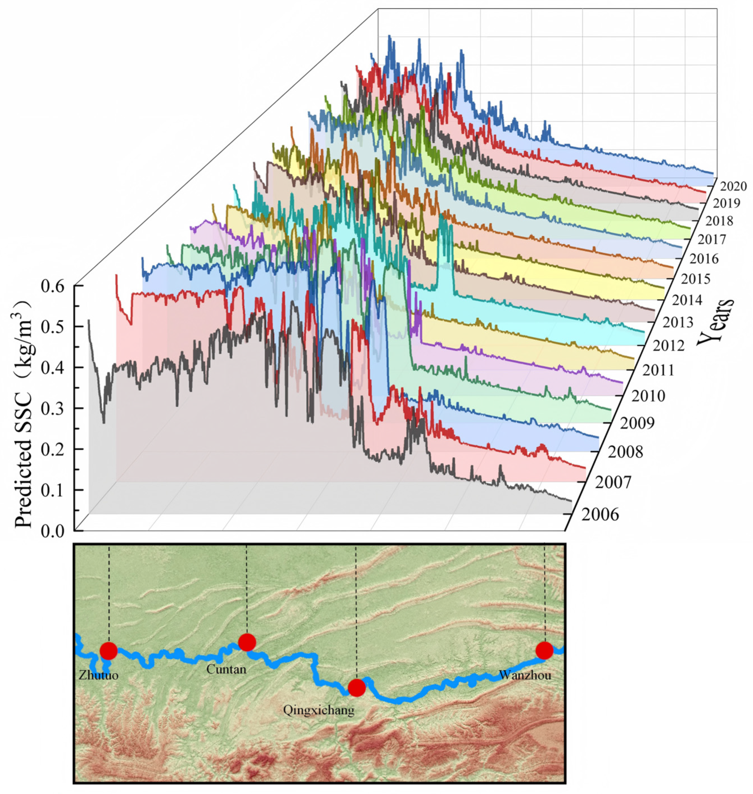
From 2006 to 2020, SSC in the mainstream of the Three Gorges Reservoir exhibited pronounced spatiotemporal differentiation. Temporally, SSC at all stations displayed a sustained declining trend with a notable interannual reduction. Spatially, SSC decreased progressively from upstream ZT toward downstream WZ (Figure 9).

$$\mathrm{L}\mathrm{o}\mathrm{n}\mathrm{g}\mathrm{i}\mathrm{t}\mathrm{u}\mathrm{d}\mathrm{i}\mathrm{n}\mathrm{a}\mathrm{l} \mathrm{d}\mathrm{e}\mathrm{c}\mathrm{l}\mathrm{i}\mathrm{n}\mathrm{e}=100\%\times {\displaystyle \frac{{\mathrm{S}\mathrm{S}\mathrm{C}}_{\mathrm{u}\mathrm{p}\mathrm{s}\mathrm{t}\mathrm{r}\mathrm{e}\mathrm{a}\mathrm{m}}-{\mathrm{S}\mathrm{S}\mathrm{C}}_{\mathrm{d}\mathrm{o}\mathrm{w}\mathrm{n}\mathrm{s}\mathrm{t}\mathrm{r}\mathrm{e}\mathrm{a}\mathrm{m}}}{{\mathrm{S}\mathrm{S}\mathrm{C}}_{\mathrm{u}\mathrm{p}\mathrm{s}\mathrm{t}\mathrm{r}\mathrm{e}\mathrm{a}\mathrm{m}}}}$$

(18)

where ${\mathrm{S}\mathrm{S}\mathrm{C}}_{\mathrm{u}\mathrm{p}\mathrm{s}\mathrm{t}\mathrm{r}\mathrm{e}\mathrm{a}\mathrm{m}}$ is the annual mean SSC at the most upstream, approximately 0.481 kg/m³, and ${\mathrm{S}\mathrm{S}\mathrm{C}}_{\mathrm{d}\mathrm{o}\mathrm{w}\mathrm{n}\mathrm{s}\mathrm{t}\mathrm{r}\mathrm{e}\mathrm{a}\mathrm{m}}$ is the annual mean SSC at the most downstream, approximately 0.03 kg/m³.

$$\mathrm{T}\mathrm{e}\mathrm{m}\mathrm{p}\mathrm{o}\mathrm{r}\mathrm{a}\mathrm{l} \mathrm{d}\mathrm{e}\mathrm{c}\mathrm{l}\mathrm{i}\mathrm{n}\mathrm{e}=100\%\times {\displaystyle \frac{{\mathrm{S}\mathrm{S}\mathrm{C}}_{2006}-{\mathrm{S}\mathrm{S}\mathrm{C}}_{2020}}{{\mathrm{S}\mathrm{S}\mathrm{C}}_{2006}}}$$

(19)

where ${\mathrm{S}\mathrm{S}\mathrm{C}}_{2006}$ is the reach-averaged SSC in 2006, approximately 0.264 kg/m³, and ${\mathrm{S}\mathrm{S}\mathrm{C}}_{2020}$ is the reach-averaged SSC in 2020, approximately 0.208 kg/m³.

Figure 9. Interannual variation in SSC along the mainstream of the Three Gorges Reservoir from 2006 to 2020.

In terms of interannual change, the annual mean SSC of the mainstream declined continuously from 2006 to 2020. At the upstream starting point, SSC was approximately 0.481 kg/m³, decreasing to roughly 0.03 kg/m³ at the downstream endpoint—a longitudinal reduction of approximately 93.8%. SSC fluctuated more markedly during 2006–2010. The sustained declining trend revealed by the remote sensing retrievals is consistent with long-term trend analyses based on hydrological station measurements. The reach-averaged SSC decreased from 0.264 kg/m³ in 2006 to 0.208 kg/m³ in 2020, a reduction of 21.2%. Spatially, SSC decreased downstream from ZT to WZ in every year, with the middle and upper reaches exhibiting substantially larger declines than the lower reach.

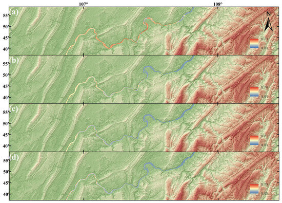
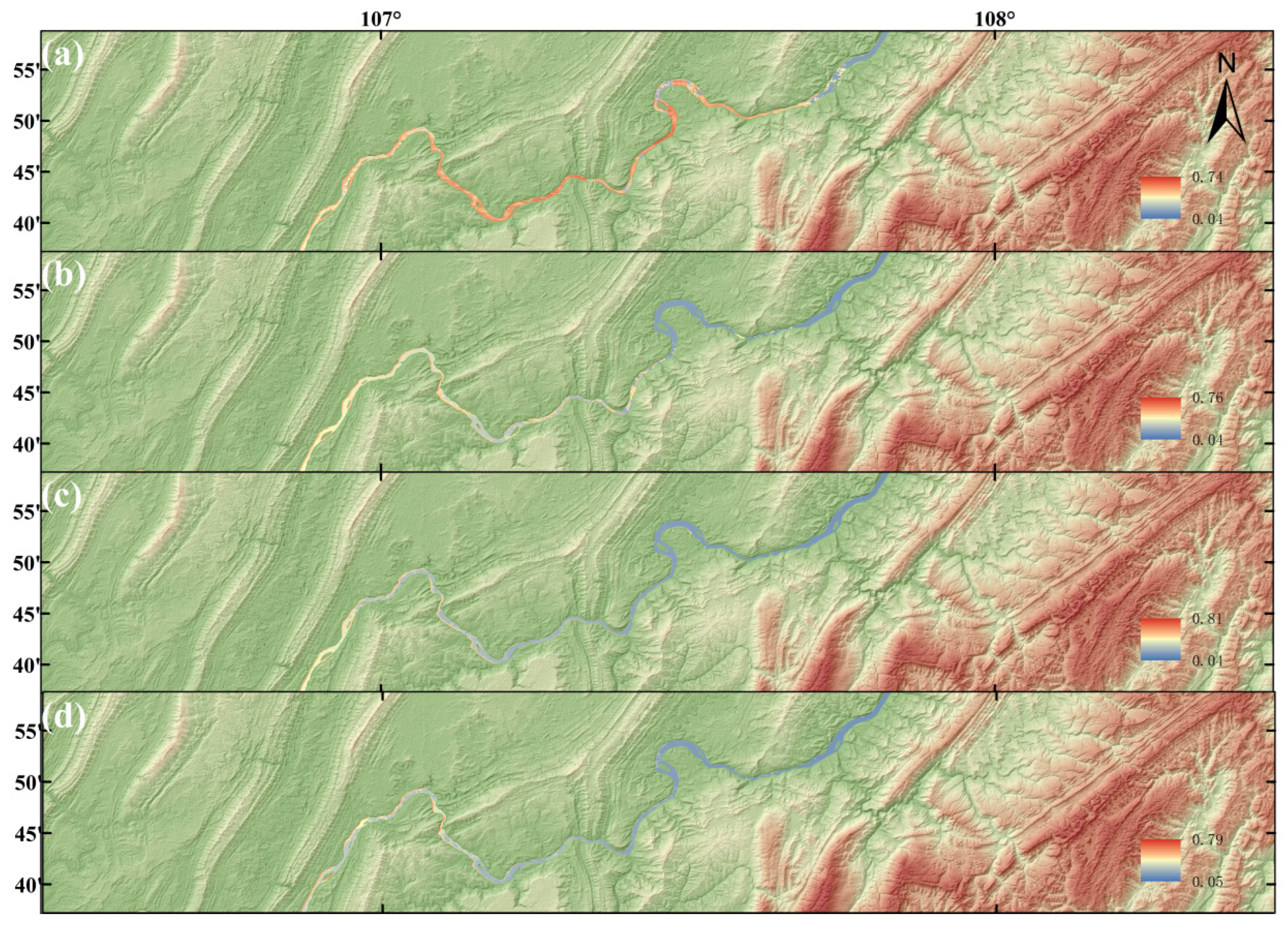
To further examine the spatial pattern, the mainstream was divided into upper, middle, and lower segments, each approximately 110 km in length and bounded by the hydrological stations (Figure 10). Taking 2006, 2010, 2016, and 2020 as representative years, the following changes were observed. In the upper segment (ZT to CT), mean annual SSC decreased from 0.377 kg/m³ in 2006 to 0.361 kg/m³ in 2020, a reduction of 4.2%. In the middle segment (CT to QXC), SSC declined from 0.320 kg/m³ in 2006 to 0.174 kg/m³ in 2020, a reduction of 45.6%. In the lower segment (QXC to WZ), SSC decreased only marginally from 0.092 kg/m³ to 0.085 kg/m³, a reduction of 7.6%, and remained consistently low throughout the period. The spatial patterns for the four representative years are illustrated.

Figure 10. Spatial patterns of SSC along the mainstream of the Three Gorges Reservoir in four representative years. (a) 2006; (b) 2010; (c) 2016; (d) 2020.

3.4.2. Wet–Dry Season SSC Differences Along the Channel

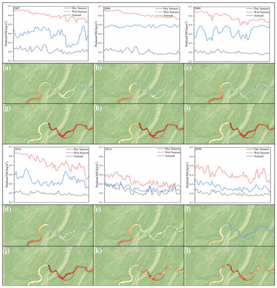
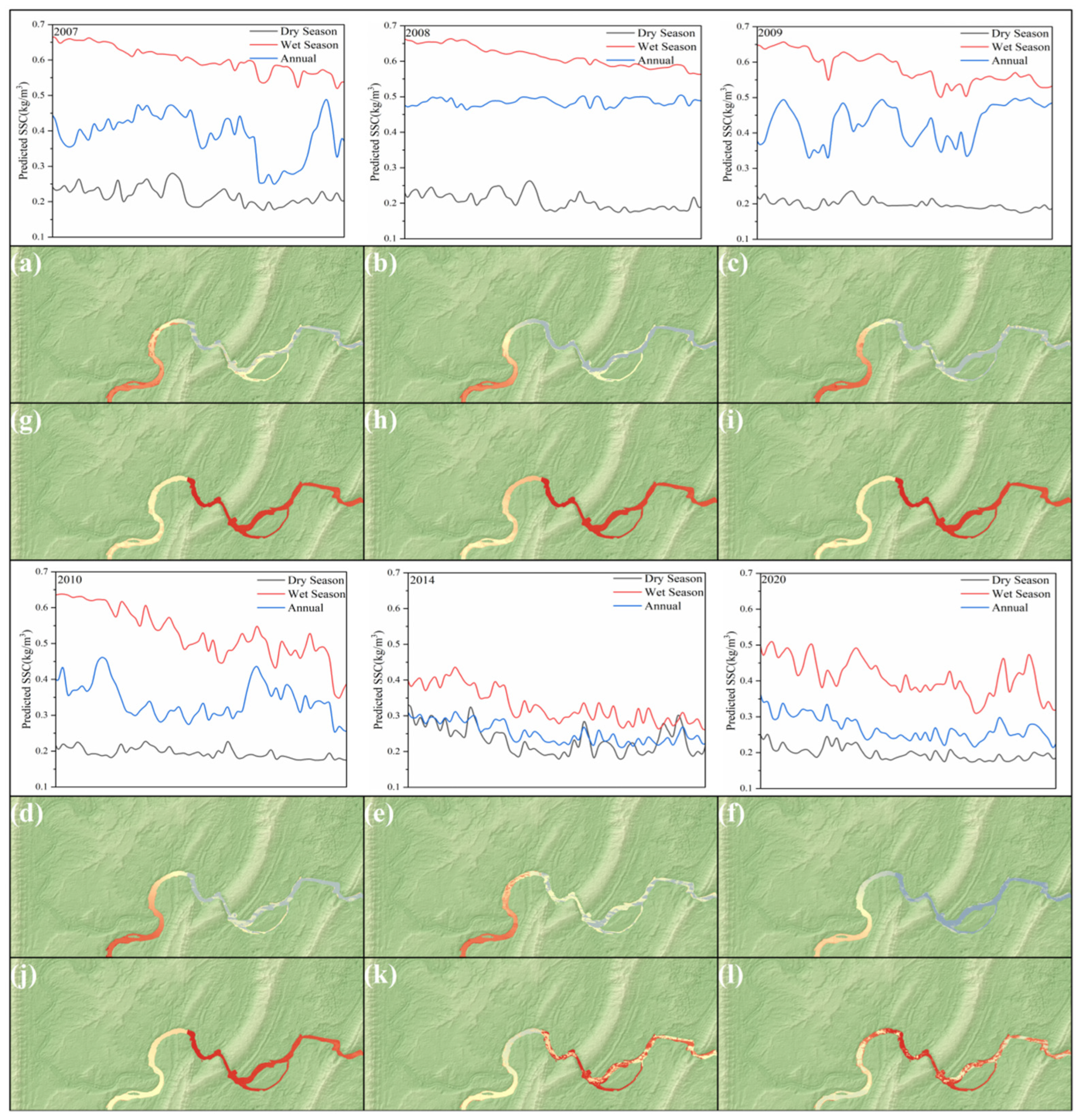
Given the pronounced channel curvature and substantial sediment deposition near CT, the reach in the vicinity of CT was selected for detailed seasonal analysis. Wet–dry season comparisons were divided into two categories: case studies of representative years (2007, 2008, 2009, 2010, 2014, and 2020) and an aggregate assessment of the remaining years (Figure 11).

Figure 11. Along-channel variations in SSC during typical years. red, black, and blue represent the dry season, wet season, and annual average, respectively. (a–f) Dry season: (a) 2007, (b) 2008, (c) 2009, (d) 2010, (e) 2014, (f) 2020. (g–l) Corresponding wet season: (g) 2007, (h) 2008, (i) 2009, (j) 2010, (k) 2014, (l) 2020. The horizontal axis represents the distance along the river reach near CT.

Along the mainstream, the longitudinal SSC gradient during the wet season was markedly steeper than during the dry season, and wet-season SSC consistently exceeded dry-season SSC, with the difference being more pronounced upstream. In the upper ZT–CT segment, the wet–dry SSC difference narrowed progressively from 0.471 kg/m³ in 2007 to 0.403 kg/m³ in 2020, a reduction of approximately 14.4%. In the downstream QXC–WZ segment, wet–dry differences from 2006 to 2019 did not exceed 0.015 kg/m³, remaining persistently small, although a difference of 0.155 kg/m³ was observed in 2020. The abnormally high value observed in 2020 resulted from a catastrophic flood that sharply increased upstream sediment supply, overwhelming the routine trapping capacity; this outcome actually suggests the model’s capability in capturing extreme hydrological events. Furthermore, the flood-season SSC response in 2014 and 2020 exhibited threefold attenuation: a systematic decline in dry-season baseline concentrations, a narrowing of wet–dry variability, and reduced downstream sediment delivery from the CT station owing to diminished upstream sediment supply and hindered transport.

For the non-representative years (2006, 2011–2013, and 2015–2019), the wet–dry differences likewise adhered to the pattern of larger upstream and smaller downstream contrasts, with wet-season values consistently higher. The upstream wet–dry amplitude gradually narrowed during the latter decade. Absolute SSC values in non-representative years fell within the range defined by the representative years, with no anomalous fluctuations observed.

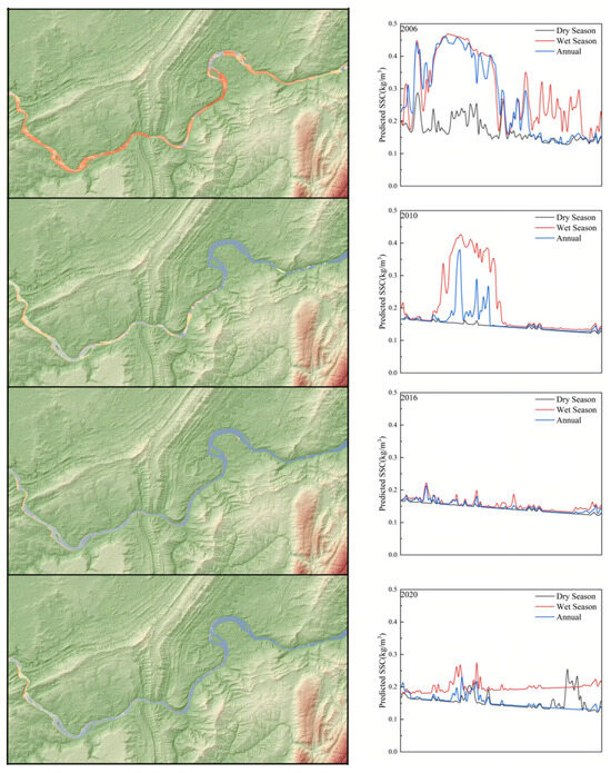
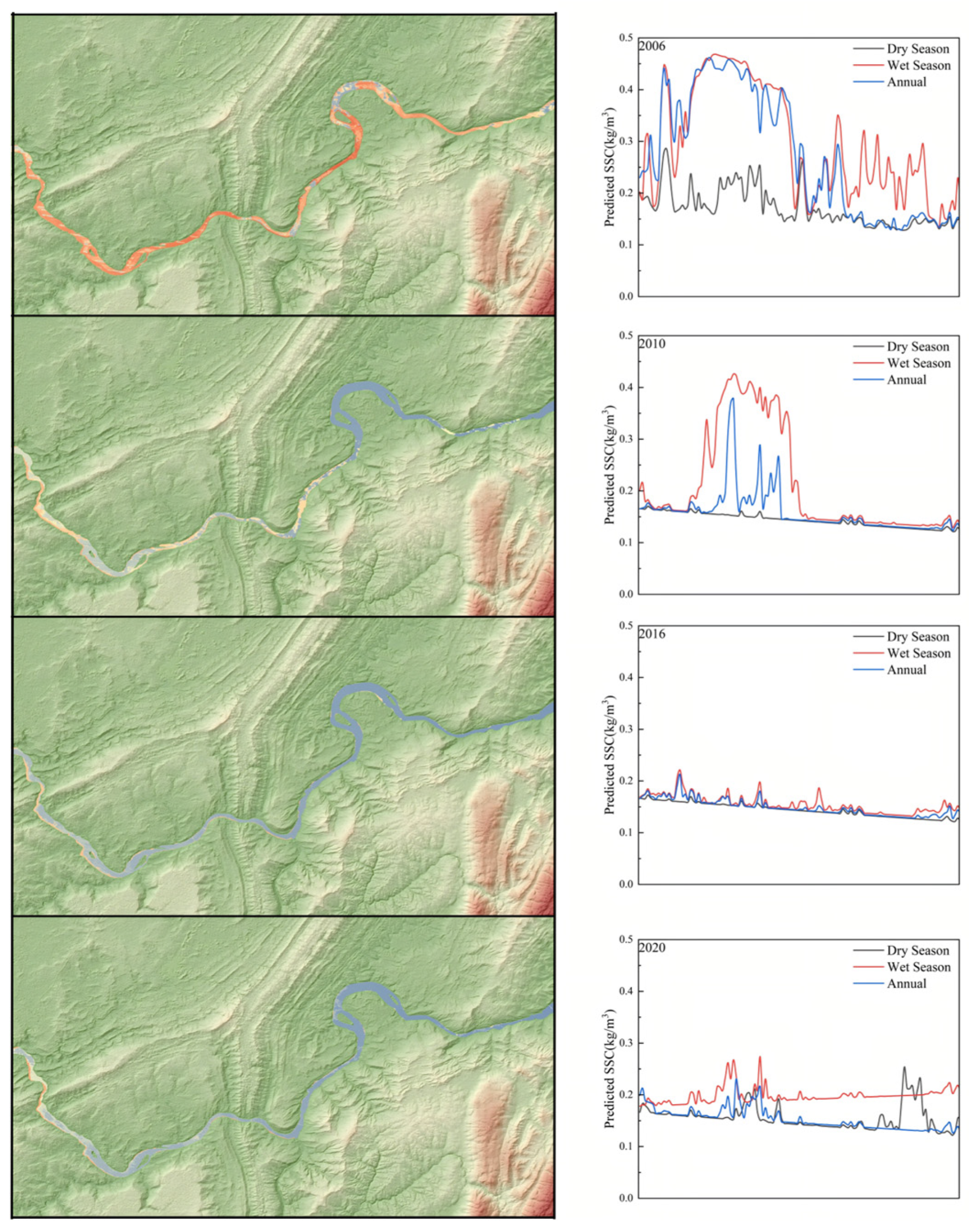
Key transition points in the CT–QXC reach were selected for analysis, with 2006, 2010, 2016, and 2020 taken as typical years. Overall, the main-stem sediment concentration declined from its 2006 peak and tended to stabilize by 2016. In 2020, it remained regionally stable at both the interannual and dry-season scales. Meanwhile, the 2020 wet season captured a substantial amount of sediment transported by an exceptional flood, thereby confirming the reliability of the model (Figure 12).

Figure 12. Red, black, and blue represent the dry season, wet season, and annual average, respectively, showing key SSC for 2006, 2010, 2016, and 2020.

4. Discussion

4.1. Spatiotemporal Data Fusion and Water Mask Index

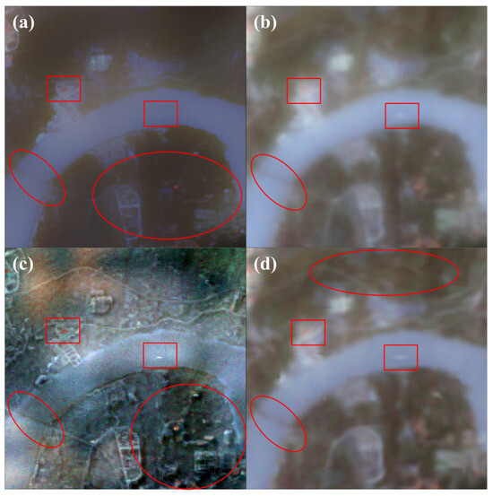
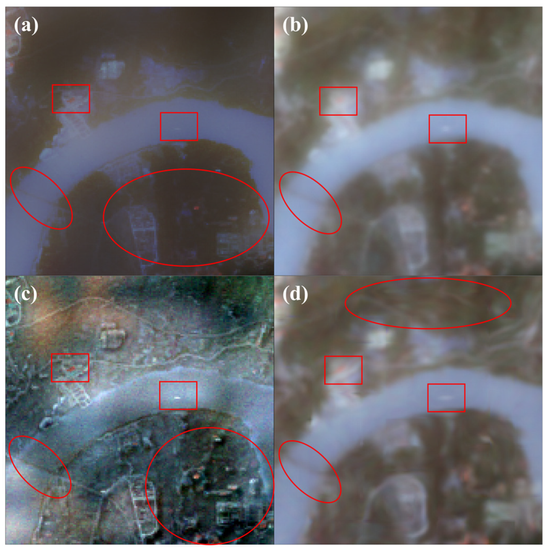
The applicability analysis of spatiotemporal fusion algorithms in the complex environment of the Three Gorges Reservoir area indicates that RASTFM achieves the optimal overall performance [34]. Its mechanistic advantages are twofold: (1) requiring only a single coarse-fine resolution image pair alleviates the scarcity constraint of cloud-free reference images in frequently cloudy regions; and (2) the change-adaptation mechanism combining non-local linear regression with spatial detail enhancement effectively captures the dynamic variations in water–land boundaries induced by reservoir regulation and the spectral temporal discrepancies caused by abrupt changes in SSC, albeit with some geometric distortion. In contrast, STARFM adheres to the assumption of temporally invariant land cover types, leading to notable degradation in radiometric fidelity within fluctuating water–land transition zones and a propensity for spectral dispersion; nevertheless, its structurally robust nature still offers a certain reference value. Although ESTARFM can partially accommodate land surface changes, its stringent requirement for multiple high-quality reference image pairs is difficult to satisfy under the typical meteorological conditions of the reservoir area. For water color remote sensing applications that rely on robust spectral-parameter quantitative relationships, the RASTFM algorithm, which prioritizes radiometric and spectral fidelity, is clearly more suitable than the alternatives. Although FSDAF requires only a single image pair and performs robustly in heterogeneous landscapes, the original algorithm’s involvement of numerous boundary pixels in spectral unmixing tends to compromise the spatial detail of the fused imagery (Figure 13).

Figure 13. Red circles indicate locations where the differences among the four fusion indices are relatively large. Spatiotemporal fusion results at the CT station. (a) STARFM, (b) ESTARFM, (c) FSDAF, (d) RASTFM. All panels are shown as RGB false-color composites.

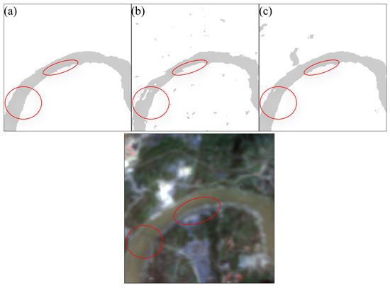
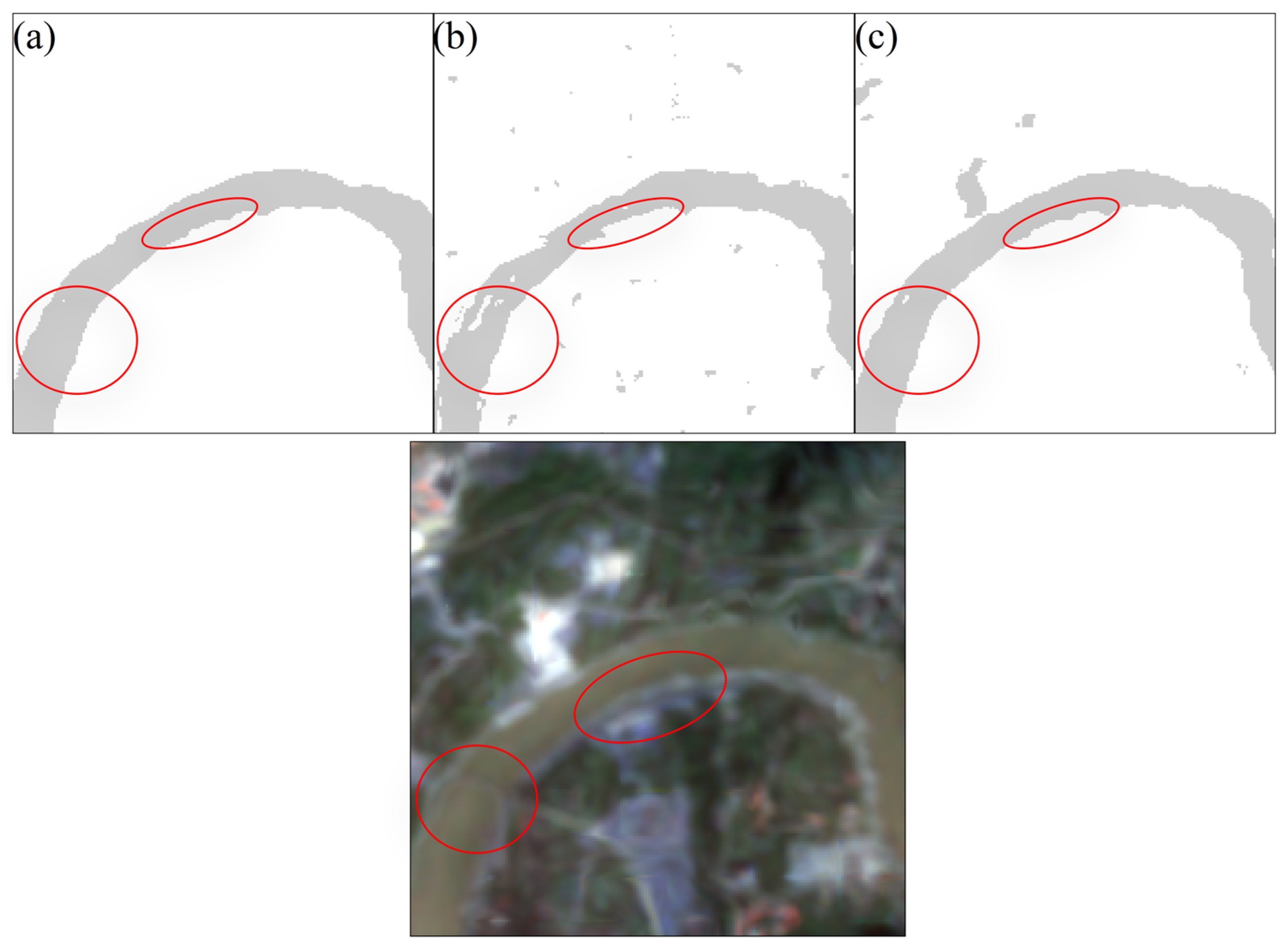
The spatial differentiation in water extraction accuracy suggests that the degree of interference from terrain shadows and urban structures constitutes the critical environmental factor determining water index performance. In reaches with intricate shorelines and severe shadow occlusion, such as ZT, CT, and QXC, MNDWI, by leveraging the strong absorption of shortwave infrared radiation by water, effectively suppresses false positives from terrain shadows and highly reflective artificial surfaces. In the open-channel reach of WZ, however, NDWI, which relies solely on green and near-infrared bands, suffices to meet the requirements for high-precision water masking. Despite the central wavelength shift between MODIS and Landsat shortwave infrared bands, the MNDWI computed from RASTFM–fused imagery maintains robust shadow-suppression capability, indicating that the efficacy of this index depends more on the overall spectral enhancement of the water target by the green–shortwave infrared band combination than on the absolute numerical matching of individual wavelengths (Figure 14). The consistently weak and unstable performance of SWI can be understood from its spectral formulation. SWI is defined as Blue + Green − NIR, which is an arithmetic rather than a ratio-based index. Arithmetic indices are intrinsically more sensitive to absolute changes in reflectance, making them vulnerable to the temporally and spatially varying scattering effects of suspended sediments in both the visible and NIR domains. Furthermore, SWI does not include a SWIR band, meaning it cannot exploit the near-zero water reflectance in SWIR for shadow suppression. As a result, the separability between water, terrain shadow, and built-up surfaces degrades under high and variable sediment loads, and the optimal segmentation threshold shifts unpredictably across stations. This mechanistic weakness explains why SWI thresholds fluctuated between 0.04 and 0.08 and why SWI consistently underperformed both MNDWI and NDWI in this sediment-rich reservoir environment.

Figure 14. Red circles indicate locations with relatively large differences among the three water body masks. Water mask results at the CT station. (a) NDWI, (b) MNDWI, (c) SWI.

For inland water quality remote sensing in topographically complex and cloud-prone regions, it is advisable to prioritize fusion algorithms with robust radiometric fidelity, such as RASTFM, to obtain high-precision imagery, and subsequently to incorporate water index threshold sensitivity analysis as a prerequisite preprocessing step for water masking to ensure the reliability of subsequent water constituent retrieval.

4.2. Mechanistic Analysis of Performance Differences Among Machine Learning Models

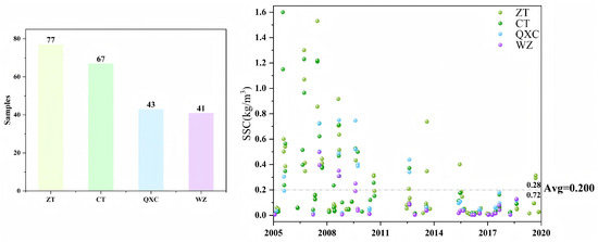
Comparison of the six machine learning models reveals that XGBoost, RF, ExtraTrees and HistGB exhibited relatively superior generalization performance in the SSC retrieval task for the Three Gorges Reservoir area, with R² values ranging from 0.60 to 0.83 [35]. This robustness can be attributed to the intrinsic compatibility between the algorithmic architectures and the data characteristics of small sample size, high noise, and skewed distribution. The study area yielded a limited effective sample size (N = 228), with spectral features significantly contaminated by cloud obscuration, terrain shadowing, and mixed-pixel effects. Furthermore, the target variable exhibited a pronounced skewed distribution, with 72% of the samples falling below the mean and only 28% above the mean. Moreover, high-concentration samples were substantially more frequent during the early years of the study period than during the later years, imposing stringent constraints on variance control and outlier tolerance for predictive models (Figure 15).

Figure 15. Sample size and sample distribution.

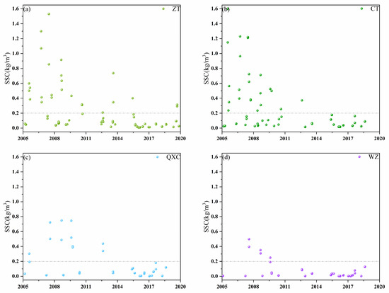
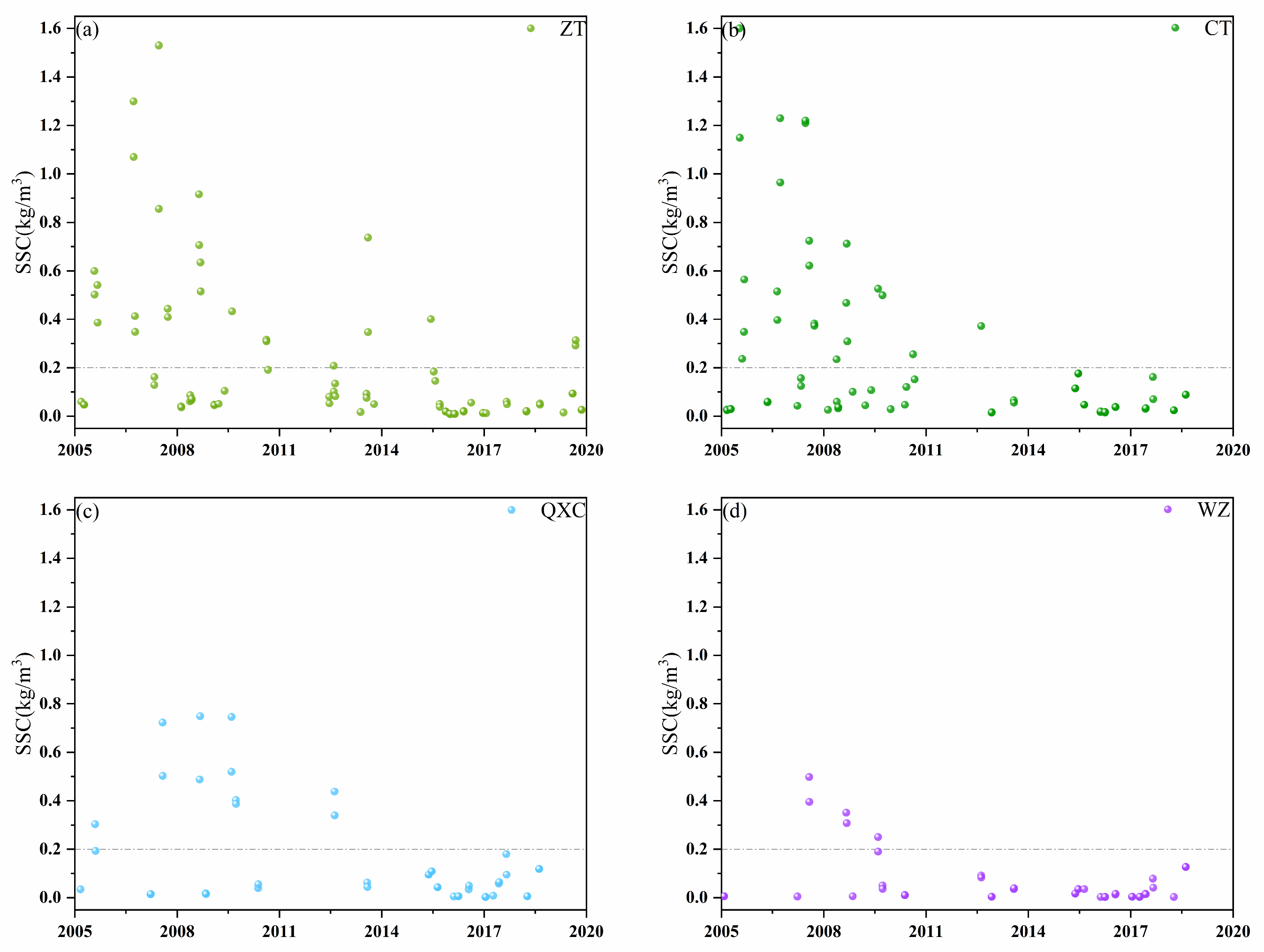
ExtraTrees, by introducing a completely randomized node-splitting threshold selection strategy, imposes a stronger stochastic perturbation within the ensemble learning framework, which essentially constitutes an implicit regularization mechanism. This mechanism effectively suppresses the tendency of individual base learners to overfit extremely high-SSC samples, thereby systematically reducing model variance at the ensemble level. HistGB, in contrast, employs a histogram-based feature discretization approximation algorithm that maps continuous spectral variables into finite bin intervals. This operation is equivalent to applying a nonparametric smoothing filter to the input feature space, filtering out random perturbation components introduced by water–land boundary mixing effects or atmospheric correction residuals, thereby compelling the model to focus on the dominant nonlinear structure of the SSC–spectral response relationship. At the QXC and WZ stations, samples were predominantly distributed below the mean. The single-sided gradient sampling strategy adopted by LightGBM, under small-sample conditions, is prone to misclassifying high-SSC anomaly observations as critical information gain sources. Combined with its leaf-wise growth mechanism, this leads to severe overfitting and model degradation, as evidenced by an R² of merely 0.14 at QXC and 0.13 at WZ [36].

To rigorously assess whether the poor performance of LightGBM stems from inadequate hyperparameter tuning, four successive tuning strategies were applied: (1) a conservative configuration with strong regularization and early stopping (Tuning—1); (2) an extremely constrained variant using decision-stump depth and minimal leaf nodes (Tuning—2); (3) an unconstrained version with all regularization removed and no early stopping (Tuning—3); and (4) a station-wise randomized search over a wide hyperparameter space (Tuning—4). The consolidated results reveal that LightGBM consistently failed to generate a positive R² at all stations (Table 7). Even under the most favorable settings, WZ station persistently yielded negative R² values, and the other three stations achieved only erratic, low R² values accompanied by large variances. The systematic failure across the full complexity spectrum demonstrates that the issue is not a matter of hyperparameter selection, but rather a fundamental incompatibility between LightGBM’s leaf-wise growth and gradient-based importance sampling with the extremely imbalanced, small-sample, and high-skew distribution of the training data. Consequently, LightGBM was excluded from the operational retrieval framework (Figure 16).

Table 7. Hyperparameter optimization of LightGBM.

St.	Turning (LightGBM)	R2	RMSE (kg/m3)	St.	Turning (LightGBM)	R2	RMSE (kg/m3)
ZT	1	−0.24 ± 0.23	0.31 ± 0.11	QXC	1	−0.92 ± 3.79	0.23 ± 0.07
	2	~	0.31 ± 0.11		2	~	0.23 ± 0.07
	3	0.49 ± 0.60	0.18 ± 0.06		3	0.54 ± 0.61	0.11 ± 0.04
	4	0.60	0.11		4	0.63	0.14
CT	1	−0.30 ± 0.41	0.37 ± 0.12	WZ	1	−0.71 ± 2.83	0.11 ± 0.05
	2	~	0.37 ± 0.12		2	~	0.11 ± 0.05
	3	0.51 ± 0.49	0.21 ± 0.08		3	−1.82 ± 7.80	0.10 ± 0.04
	4	0.56	0.223		4	−0.58	0.07

Figure 16. Distribution of independent samples at the four stations: (a) ZT, (b) CT, (c) QXC, (d) WZ.

Leveraging the RASTFM spatiotemporally fused image reconstruction dataset in conjunction with the selected optimal machine learning model framework yields retrieval accuracy that demonstrates certain advantages over conventional empirical regression paradigms. Furthermore, in terms of characterizing spatial heterogeneity, the approach successfully captures the spatiotemporal differentiation modalities of “higher concentrations near banks than in mid-channel” and “higher concentrations in summer than in spring.” Concurrently, the along-channel declining trend in SSC and the wet–dry seasonal differences revealed by the retrieval results provide quantitative remote sensing empirical evidence for elucidating the hydrological regulation mechanisms governing SSC evolution in the reservoir area.

4.3. Spatiotemporal Evolution Characteristics of SSC

Recent advances in remote sensing have enabled the recognition of estuarine turbidity maxima at global scales, yet long-term, continuous monitoring in reservoir backwater zones remains a challenge.

The in situ dataset used in this study exhibits an imbalanced distribution across concentration ranges, with far fewer samples in the high-SSC regime than in the low-to-moderate regime. To evaluate and mitigate the potential impact of this imbalance on model training and validation, we adopted the following strategies. First, a logarithmic transformation was applied to the target variable prior to model training, which reduced the disproportionate influence of sparse high-value samples on the loss function and helped the model learn spectral–concentration relationships more evenly across concentration intervals. Second, during validation, all samples were stratified into low, medium, and high tiers according to concentration, and accuracy metrics (R², RMSE, and MAPE) were reported separately for each tier. The stratified results confirmed that the model performs robustly in the well-represented low-to-medium range; although the absolute error increased in the high-concentration tier, the relative error remained acceptable. Since the primary application scenarios of this study focus on low-to-medium turbidity waters, the imbalanced sample distribution does not appreciably undermine the reliability of the main conclusions. Future work with an expanded high-concentration dataset would further strengthen model applicability under extremely turbid conditions.

Time-series analysis of the reservoir retrievals indicates that, with the concentrated commissioning of cascade reservoirs in the lower Changjiang River between 2012 and 2014 serving as a pivotal transitional period, the sediment transport processes in the Three Gorges Reservoir area exhibit a distinct phase transition. Xu and Milliman [37] noted a drastic decline in seasonal sediment discharge from the Changjiang River after the impoundment of the Three Gorges Dam. Furthermore, Ren et al. [38] found that the construction of cascade reservoirs significantly impacts peak sediment transport during flood events, leading to more pronounced sediment hysteresis. These findings corroborate our observations of a threefold attenuation in the flood-season SSC response: a systematic decline in dry-season baseline concentrations, a significant narrowing of wet–dry variability, and impeded long-distance downstream transport of high-SSC water bodies after 2014.

Sediment trapping by upstream cascade reservoirs has led to a sharp reduction in flood-season sediment inflow, with a concurrent decline in dry-season background concentrations. Between 2007 and 2010, large cascade hydropower stations on the lower Changjiang River, such as Xiangjiaba and Xiluodu, had not yet commenced impoundment, and flood events in the upper Changjiang River still delivered substantial suspended sediment loads into the Three Gorges Reservoir, resulting in pronounced “flood peak–sediment peak synchronization” transport processes. Between 2012 and 2014, Xiangjiaba and Xiluodu successively began water storage, and their significant sediment trapping effect substantially reduced the sediment load entering the Three Gorges Reservoir. The sustained decline in upstream sediment supply has not only directly diminished the magnitude of flood-season sediment peaks but has also systematically lowered the background SSC of the reservoir water body during the dry season. The comprehensive reduction in SSC observed in the upstream reach of CT in 2014 and 2020 constitutes direct evidence of weakened upstream “source” input. Huang et al. [39] also noted unexpected sedimentation patterns both upstream and downstream of the TGR, emphasizing the future risks of sediment deposition and channel scour. Our findings of a migrating deposition center and altered sediment transport regimes directly reflect these large-scale geomorphic changes driven by the combined operation of the Three Gorges Dam and upstream cascade reservoirs.

The deposition center within the fluctuating backwater zone of the Three Gorges Reservoir has migrated upstream, with the reach near the CT station emerging as a critical sediment interception node. Following the impoundment of the Three Gorges Reservoir, hydrodynamic conditions within the reservoir area have been altered, manifesting as reduced flow velocity, increased water depth, and diminished sediment transport capacity. With the continuous decline in upstream sediment supply, the locus of sediment deposition within the reservoir has gradually shifted toward the tail region of the backwater zone. CT station, situated downstream of the confluence of the Jialing River and the Changjiang River mainstream, constitutes the key control section for the upper segment of the Three Gorges Reservoir’s fluctuating backwater zone. After the reservoir first achieved 175 m experimental impoundment in 2010, the backwater terminus extended further upstream, and flow velocities in the reach near the CT station decreased markedly, substantially enhancing sediment deposition efficiency [40]. Consequently, this section transitioned from an early-stage “sediment transport” regime toward a “sediment deposition” regime. During flood seasons, the limited incoming sediment load undergoes preferential deposition of coarse particles upon passing the CT station; although the remaining fine particles may continue downstream transport, their concentration is already substantially attenuated, making it difficult to form pronounced high-SSC peaks at the QXC station.

The narrowing of wet–dry SSC variability fundamentally reflects the rebalancing of the “source–sink” relationship. During the 2007–2010 period of abundant upstream sediment supply, flood events could drive substantial sediment loads into the reservoir and convey them downstream, generating pronounced wet–dry contrasts. In contrast, during the 2014–2020 period of sharply reduced upstream sediment supply, even when basin-scale major floods occurred, the available sediment sources had already been substantially diminished. Moreover, preferential interception in the reach upstream of the CT station severely compressed the potential for flood-season SSC elevation, resulting in markedly narrowed wet–dry variability. The evolutionary trend of progressively narrowing wet–dry amplitudes derived from this study corroborates the strong regulatory control exerted by coordinated reservoir group operations on sediment transport processes within the reservoir area.

4.4. Uncertainty Analysis

The uncertainties in this study primarily originate from the following four sources: (1) Although the RASTFM algorithm achieved the optimal comprehensive performance, temporal differences in water–sediment conditions arising from varying seasonal separations between reference and target images, residual misregistration, biases in coarse-pixel heterogeneity assumptions, and residual cloud/shadow contamination introduce localized spectral reconstruction uncertainties, particularly in water–land boundary zones and high-SSC areas. (2) Threshold segmentation based on MNDWI and NDWI is influenced by the continuous response characteristics of water–land transition zones and temporal discrepancies relative to the JRC reference dataset. Boundary mixed-pixel class flipping and residual shadow interference constitute the primary sources of sample contamination. (3) The limited sample size of only 228 matched pairs relative to an initial pool of 227 candidate features creates a “large p, small n” scenario that inherently elevates the risk of chance correlations and overfitting. Although the Pearson-based feature screening reduced the feature space to 20 dimensions, this linear filter cannot guarantee the retention of features that interact with SSC through complex nonlinear mechanisms. Consequently, some predictive power may have been lost during feature reduction, and the remaining features may still contain residual redundancy. The standard deviation of cross-validation R² reaching 0.34 at certain stations further reflects model sensitivity to data partitioning under such sample-constrained conditions. (4) Spectral errors from fusion are amplified through the nonlinear transformation of water indices; water extraction errors propagate into and contaminate the retrieval sample set, ultimately resulting in significantly widened prediction confidence intervals during high-SSC flood periods. Although the soft-constraint post-processing strategy can suppress anomalous predictions, the empirical determination of the threshold parameter α still entails subjective uncertainty.

5. Conclusions

This study established a long-term SSC remote sensing monitoring framework encompassing “spatiotemporal fusion–water extraction–feature construction–machine learning retrieval.” Within this framework, we conducted multi-source data fusion algorithm optimization, water index threshold sensitivity analysis, machine learning model evaluation under small-sample conditions, and spatiotemporally continuous SSC retrieval for the Three Gorges Reservoir area from 2006 to 2020. The principal findings are as follows:

(1) Of the four spatiotemporal fusion algorithms compared, RASTFM performed best in spectral fidelity and data usability, providing a reliable data source for frequently cloudy regions.

(2) MNDWI was more resistant to interference from terrain shadows and urban infrastructure, while NDWI sufficed for accurate water masking in open channels. Station-specific threshold optimization is essential for extraction accuracy.

(3) With limited samples and high noise, ExtraTrees, HistGB, and XGBoost all generalized more robustly than LightGBM. ExtraTrees and HistGB showed the most consistent inter-station performance, effectively reducing overfitting and enabling high-precision SSC retrieval.

(4) The long-term SSC record reveals a significant declining trend in mainstream SSC in the Three Gorges Reservoir area from 2006 to 2020, decreasing from upstream ZT to downstream WZ. Wet–dry seasonal variability also narrowed as upstream cascade reservoirs came online. This temporal link suggests that upstream cascade reservoirs have substantially reduced sediment input to the upper and middle reaches, while the lower perennial backwater zone is dominated by local depositional processes under reduced flow velocity. Isolating the individual contributions of upstream damming and local impoundment effects still requires further study.

References

- Zhang, Z.; Ao, Z.; Wu, W.; Wang, Y.; Xin, Q. Developing a Multi-Scale Convolutional Neural Network for Spatiotemporal Fusion to Generate MODIS-like Data Using AVHRR and Landsat Images. Remote Sens. 2024, 16, 1086. [Google Scholar] [CrossRef]
- Li, J.; Wang, G.; Sun, S.; Ma, J.; Guo, L.; Song, C.; Lin, S. Mapping and Reconstruct Suspended Sediment Dynamics (1986–2021) in the Source Region of the Yangtze River, Qinghai-Tibet Plateau Using Google Earth Engine. Remote Sens. Environ. 2025, 317, 114533. [Google Scholar] [CrossRef]
- Tao, H.; Song, K.; Wen, Z.; Liu, G.; Shang, Y.; Fang, C.; Wang, Q. Remote Sensing of Total Suspended Matter of Inland Waters: Past, Current Status, and Future Directions. Ecol. Inform. 2025, 86, 103062. [Google Scholar] [CrossRef]
- Stull, T.; Ahmari, H. Estimation of Suspended Sediment Concentration along the Lower Brazos River Using Satellite Imagery and Machine Learning. Remote Sens. 2024, 16, 1727. [Google Scholar] [CrossRef]
- Duan, M. Research Progress and Prospects of Remote Sensing on Suspended Sediment in River Water. Adv. Earth Sci. 2023, 38, 675. [Google Scholar] [CrossRef]
- Di Trapani, A.; Corbari, C.; Mancini, M. Effect of the Three Gorges Dam on Total Suspended Sediments from MODIS and Landsat Satellite Data. Water 2020, 12, 3259. [Google Scholar] [CrossRef]
- Gao, F.; Masek, J.; Schwaller, M.; Hall, F. On the Blending of the Landsat and MODIS Surface Reflectance: Predicting Daily Landsat Surface Reflectance. IEEE Trans. Geosci. Remote Sens. 2006, 44, 2207–2218. [Google Scholar] [CrossRef]
- Foody, G.M. Assessing the Accuracy of Land Cover Change with Imperfect Ground Reference Data. Remote Sens. Environ. 2010, 114, 2271–2285. [Google Scholar] [CrossRef]
- Zhao, Y.; Huang, B.; Song, H. A Robust Adaptive Spatial and Temporal Image Fusion Model for Complex Land Surface Changes. Remote Sens. Environ. 2018, 208, 42–62. [Google Scholar] [CrossRef]
- McFeeters, S.K. The Use of the Normalized Difference Water Index (NDWI) in the Delineation of Open Water Features. Int. J. Remote Sens. 1996, 17, 1425–1432. [Google Scholar] [CrossRef]
- Xu, H. Modification of Normalised Difference Water Index (NDWI) to Enhance Open Water Features in Remotely Sensed Imagery. Int. J. Remote Sens. 2006, 27, 3025–3033. [Google Scholar] [CrossRef]
- Erten, G. A Machine Learning Framework for Estimating Suspended Sediment Continental United States Using 40 Years of Landsat Observations. Sci. Total Environ. 2025, 1006, 180941. [Google Scholar] [CrossRef] [PubMed]
- Zaghian, S.; Mohammadzadeh, A.; Ghorbanian, A.; Bovolo, F.; Niroumand-Jadidi, M. Enhancing Suspended Sediment Concentration Retrieval by Integrating Thermal Infrared and Optical Bands of Landsat-8 and Machine Learning Algorithms. Int. J. Remote Sens. 2023, 44, 5814–5844. [Google Scholar] [CrossRef]
- Hu, J.; Miao, C.; Zhang, X.; Kong, D. Retrieval of Suspended Sediment Concentrations Using Remote Sensing and Machine Learning Methods: A Case Study of the Lower Yellow River. J. Hydrol. 2023, 627, 130369. [Google Scholar] [CrossRef]
- Breiman, L. Random Forests. Mach. Learn. 2001, 45, 5–32. [Google Scholar] [CrossRef]
- Chen, T.; Guestrin, C. XGBoost: A Scalable Tree Boosting System. In Proceedings of the 22nd ACM SIGKDD International Conference on Knowledge Discovery and Data Mining; ACM: San Francisco, CA, USA, 2016; pp. 785–794. [Google Scholar]
- Geurts, P.; Ernst, D.; Wehenkel, L. Extremely Randomized Trees. Mach. Learn. 2006, 63, 3–42. [Google Scholar] [CrossRef]
- Guolin Ke, Q.M. LightGBM: A Highly Efficient Gradient Boosting Decision Tree. In Proceedings of the 31st International Conference on Neural Information Processing Systems; Curran Associates, Inc.: Long Beac, CA, USA, 2017; pp. 1–9. [Google Scholar]
- Lu, S.; Jing, J.; Yang, L.; Nie, B.; Feng, L.; He, X.; Zhou, J. FSDFormer: A Frequency-Selected Differential Fusion Transformer for Remote Sensing Image Spatiotemporal Fusion. IEEE Trans. Geosci. Remote Sens. 2025, 63, 5406818. [Google Scholar] [CrossRef]
- Sun, J.; Shen, J.; Li, H.; Wang, H.; Ren, A.; Zhou, X.; Yong, B. QCL-LNF: A Spatiotemporal Quantum CNN-LSTM Model for Long-Term NDVI Forecasting. IEEE Trans. Geosci. Remote Sens. 2025, 63, 4416914. [Google Scholar] [CrossRef]
- Qiao, X.; Huang, W. Ocean Surface Wind Speed Estimation From GNSS-R Data Using Physics-Informed Attention-Aided Convolutional Neural Network. IEEE Trans. Geosci. Remote Sens. 2025, 63, 4210116. [Google Scholar] [CrossRef]
- Tripathy, K.P.; Mishra, A.K. Deep Learning in Hydrology and Water Resources Disciplines: Concepts, Methods, Applications, and Research Directions. J. Hydrol. 2024, 628, 130458. [Google Scholar] [CrossRef]
- Wang, C.; Zhou, C.; Zhou, X.; Duan, M.; Yan, Y.; Wang, J.; Wang, L.; Jia, K.; Sun, Y.; Wang, D.; et al. A Universal Method to Recognize Global Big Rivers Estuarine Turbidity Maximum from Remote Sensing. ISPRS J. Photogramm. Remote Sens. 2025, 220, 509–523. [Google Scholar] [CrossRef]
- Yang, S.L.; Milliman, J.D.; Xu, K.H.; Deng, B.; Zhang, X.Y.; Luo, X.X. Downstream Sedimentary and Geomorphic Impacts of the Three Gorges Dam on the Yangtze River. Earth-Sci. Rev. 2014, 138, 469–486. [Google Scholar] [CrossRef]
- Yang, H.F.; Yang, S.L.; Xu, K.H.; Milliman, J.D.; Wang, H.; Yang, Z.; Chen, Z.; Zhang, C.Y. Human Impacts on Sediment in the Yangtze River: A Review and New Perspectives. Glob. Planet. Change 2018, 162, 8–17. [Google Scholar] [CrossRef]
- Yang, L.; Zeng, S.; Xia, J.; Wang, Y.; Huang, R.; Chen, M. Effects of the Three Gorges Dam on the Downstream Streamflow Based on a Large-Scale Hydrological and Hydrodynamics Coupled Model. J. Hydrol. Reg. Stud. 2022, 40, 101039. [Google Scholar] [CrossRef]
- China Planning Press. Specification for Suspended Sediment Measurement in Rivers; China Planning Press: Beijing, China, 2015.
- Cui, T.; Zhang, J.; Groom, S.; Sun, L.; Smyth, T.; Sathyendranath, S. Validation of MERIS Ocean-Color Products in the Bohai Sea: A Case Study for Turbid Coastal Waters. Remote Sens. Environ. 2010, 114, 2326–2336. [Google Scholar] [CrossRef]
- Zhu, X.; Chen, J.; Gao, F.; Chen, X.; Masek, J.G. An Enhanced Spatial and Temporal Adaptive Reflectance Fusion Model for Complex Heterogeneous Regions. Remote Sens. Environ. 2010, 114, 2610–2623. [Google Scholar] [CrossRef]
- Zhu, X.; Helmer, E.H.; Gao, F.; Liu, D.; Chen, J.; Lefsky, M.A. A Flexible Spatiotemporal Method for Fusing Satellite Images with Different Resolutions. Remote Sens. Environ. 2016, 172, 165–177. [Google Scholar] [CrossRef]
- Xu, Q.; Guo, Y.; Chen, W.; Ji, G.; Shi, L.; Li, Y.; Zheng, Z.; Sun, C.; Zhu, H. Comprehensive Assessment of Spatiotemporal Fusion Methods in Inland Water Monitoring. GISci. Remote Sens. 2024, 61, 2343200. [Google Scholar] [CrossRef]
- Guo, D.; Li, Z.; Gao, X.; Gao, M.; Yu, C.; Zhang, C.; Shi, W. RealFusion: A Reliable Deep Learning-Based Spatiotemporal Fusion Framework for Generating Seamless Fine-Resolution Imagery. Remote Sens. Environ. 2025, 321, 114689. [Google Scholar] [CrossRef]
- Cai, C.; Liu, L.; Wang, Z.; Pang, W.; Bai, C.; Zhang, H. Retrieval of Non-Optical Active Water Quality Parameters in Complex Lake Environments Using a Novel Zoning-Based Ensemble Modeling Strategy. Ecol. Indic. 2025, 176, 113723. [Google Scholar] [CrossRef]
- Zheng, D.; Lv, A. MosaicFormer: A Novel Approach to Remote Sensing Spatiotemporal Data Fusion for Lake Water Monitors. Remote Sens. 2025, 17, 1138. [Google Scholar] [CrossRef]
- Kundu, S.; Swarnkar, S.; Agarwal, A. Bayesian-Optimized Recursive Machine Learning for Predicting Human-Induced Changes in Suspended Sediment Transport. Environ. Monit. Assess. 2025, 197, 603. [Google Scholar] [CrossRef] [PubMed]
- Fan, J.; Li, R.; Zhao, M.; Pan, X. A BiLSTM-Based Hybrid Ensemble Approach for Forecasting Suspended Sediment Concentrations: Application to the Upper Yellow River. Land 2025, 14, 1199. [Google Scholar] [CrossRef]
- Xu, K.; Milliman, J.D. Seasonal Variations of Sediment Discharge from the Yangtze River before and after Impoundment of the Three Gorges Dam. Geomorphology 2009, 104, 276–283. [Google Scholar] [CrossRef]
- Ren, J.; Zhao, M.; Zhang, W.; Xu, Q.; Yuan, J.; Dong, B. Impact of the Construction of Cascade Reservoirs on Suspended Sediment Peak Transport Variation during Flood Events in the Three Gorges Reservoir. CATENA 2020, 188, 104409. [Google Scholar] [CrossRef]
- Huang, Y.; Wang, J.; Yang, M. Unexpected Sedimentation Patterns Upstream and Downstream of the Three Gorges Reservoir: Future Risks. Int. J. Sediment Res. 2019, 34, 108–117. [Google Scholar] [CrossRef]
- Liu, J.; Yang, Y.; Li, M.; Liu, X.; Ji, C.; Liu, Y. Study on the Evolution of the Sandy-Gravel Riverbed and the Characteristics of Channel Hydrodynamic Force after the Operation of the Three Gorges Project. Front. Water 2025, 7, 1579728. [Google Scholar] [CrossRef]
Disclaimer/Publisher’s Note: The statements, opinions and data contained in all publications are solely those of the individual author(s) and contributor(s) and not of MDPI and/or the editor(s). MDPI and/or the editor(s) disclaim responsibility for any injury to people or property resulting from any ideas, methods, instructions or products referred to in the content. |
© 2026 by the authors. Licensee MDPI, Basel, Switzerland. This article is an open access article distributed under the terms and conditions of the Creative Commons Attribution (CC BY) license.