3D Gaussian Splatting for Large-Scale Remote Sensing: A PRISMA-Informed Scoping Review of Scalability, Geometric Reliability, and Benchmarking Across UAV/Aerial and Satellite Imagery

Highlights

What are the main findings?

• A faceted four-axis taxonomy organizes remote-sensing 3DGS by platform, sensor model, scalability strategy, and geometric supervision.
• Existing scaling strategies improve efficiency, but metric reliability still depends on sensor modeling, geometric constraints, and product-level evaluation.

What are the implications of the main findings?

• UAV/aerial and satellite 3DGS should be evaluated with platform-aware, supervision-explicit, and multi-metric protocols rather than a single undifferentiated ranking.
• The proposed benchmark framework links visual fidelity, computational cost, metric geometry, product utility, and failure behavior for more reproducible remote-sensing evaluation.

Abstract

3D Gaussian Splatting (3DGS) offers efficient explicit rendering, but large-scale remote-sensing use remains fragmented across UAV/aerial photogrammetry, satellite reconstruction, large-scene scaling, surface modeling, and geospatial evaluation. We present a Preferred Reporting Items for Systematic Reviews and Meta-Analyses (PRISMA)-informed scoping review based on 55 core studies identified through Web of Science, Scopus, IEEE Xplore, and supplementary searches completed on 3 June 2026. A faceted taxonomy organizes the literature by platform, sensor model, scalability strategy, and geometric supervision. The synthesis shows that partitioning, hierarchy, compression, and feed-forward inference improve scalability but do not guarantee metric geometry. Reliable deployment additionally requires sensor-consistent projection, geometric or georeferencing constraints, explicit supervision labels, and product-level evaluation. In control-point-free settings, internal consistency should be distinguished from independently validated accuracy. We therefore propose a platform-aware benchmark framework that jointly records visual fidelity, computational cost, metric geometry, product utility, failure behavior, and reproducibility metadata for UAV/aerial, satellite, and hybrid settings.

1. Introduction

Large-scale remote sensing increasingly requires reusable 3D representations for visualization, measurement, orthophoto production, surface modeling, and geospatial analysis. Plausible novel view synthesis (NVS) alone is insufficient: useful models must preserve geometry, tolerate appearance change, and support products such as digital surface models (DSMs), heights, and georeferenced measurements [1,2,3,4,5,6].

Neural Radiance Fields (NeRFs) established differentiable scene reconstruction, while S-NeRF, Sat-NeRF, and EO-NeRF exposed the importance of shadows, transient objects, rational polynomial coefficient (RPC) cameras, and geometric constraints in satellite imagery [7,8,9,10]. 3DGS replaces repeated ray sampling with explicit anisotropic Gaussians and rasterization, but its vanilla form does not address push-broom/RPC sensors, georeferencing, large-area scaling, or mapping-grade geometry [1]. Subsequent work has combined partitioning, level-of-detail (LoD) rendering, compression, and generalizable prediction with LiDAR guidance, camera refinement, temporal or semantic modeling, surface constraints, and product-oriented evaluation [11,12,13,14,15,16,17,18,19,20,21,22,23,24,25,26,27].

This PRISMA-informed scoping review contributes a 55-study corpus, a faceted taxonomy separating observation conditions from methodological responses, a supervision-aware synthesis of scalability and geometry, and a benchmark reporting framework covering tracks, costs, metrics, failures, and machine-readable metadata. It does not claim the underlying LiDAR, RPC, surface, or georeferencing techniques as new; it organizes them for more defensible comparison across UAV/aerial and satellite settings.

2. Review Design, PRISMA Methodology, and Analytical Framework

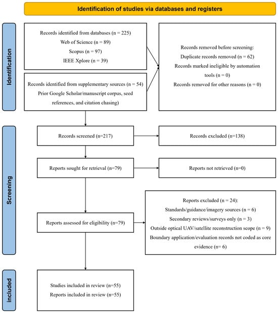
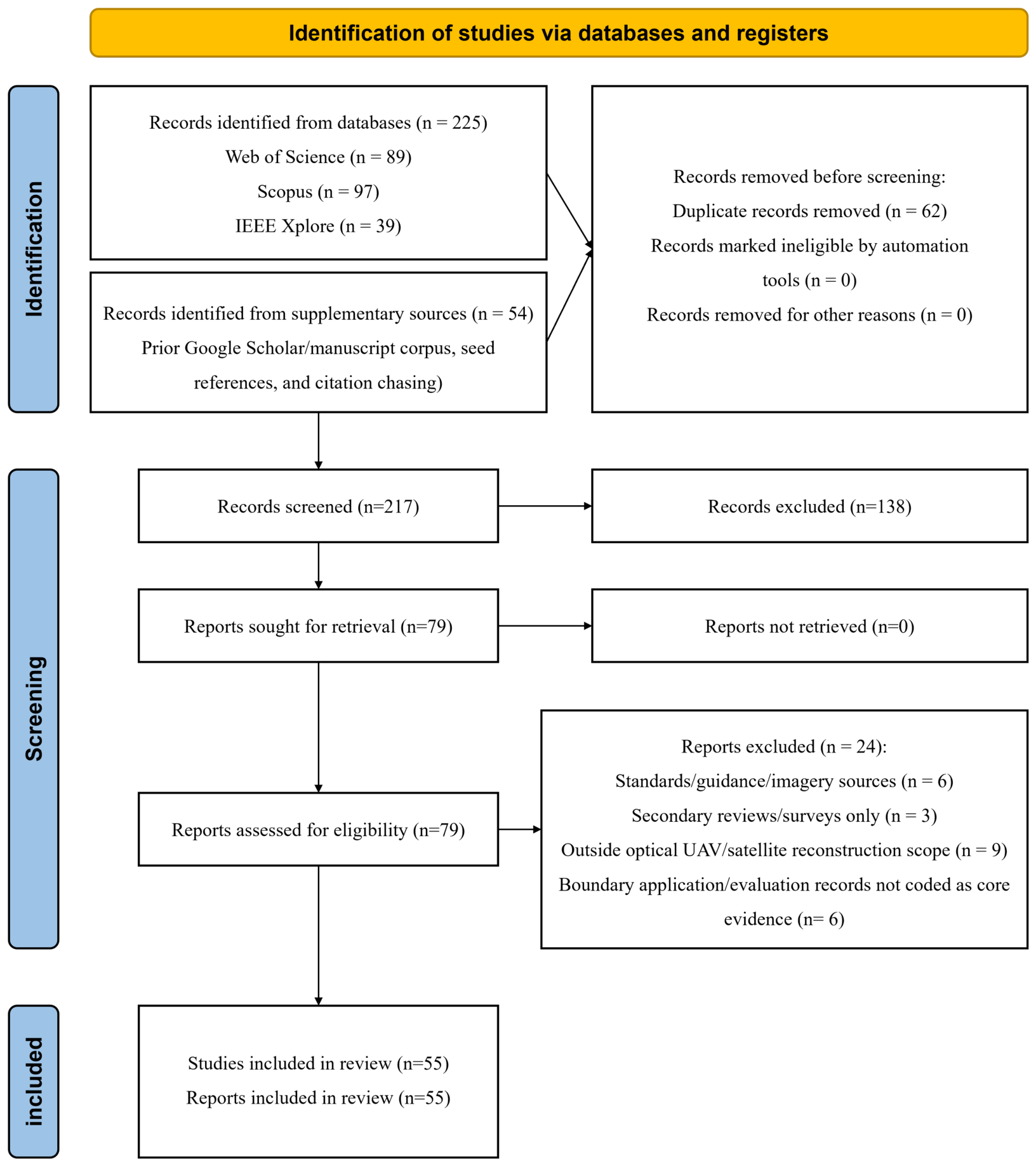
This article is a PRISMA-informed scoping review rather than a quantitative meta-analysis. PRISMA 2020 is used to report identification, screening, eligibility, inclusion, and protocol status transparently [28]. Supplementary File S1 contains the checklist and Figure 1 summarizes selection.

Figure 1. PRISMA 2020 flow diagram for the identification, screening, eligibility assessment, and inclusion of studies in the 55-study core corpus.

2.1. Review Questions

The review asks: (1) how 3DGS is adapted to UAV/aerial and satellite sensing; (2) which scalability, sensor-model, and geometric constraints govern reliable large-scale use; and (3) which benchmark and reproducibility gaps prevent fair comparison.

2.2. Review Scope

We include explicit Gaussian scene representations and closely related radiance-field antecedents relevant to optical UAV/aerial and satellite image-based reconstruction. Hybrid aerial–ground work is retained when it informs scale, sensor modeling, fusion, or geospatial products. The scope excludes SAR, hyperspectral, thermal, LiDAR-only, underwater, and non-image reconstruction except as methodological context. General 3DGS and sparse-view surveys already cover the broader field [29,30,31]; this review focuses on the tension between rendering efficiency and sensor-consistent, product-level geometry.

2.3. Information Sources and Search Strategy

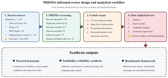
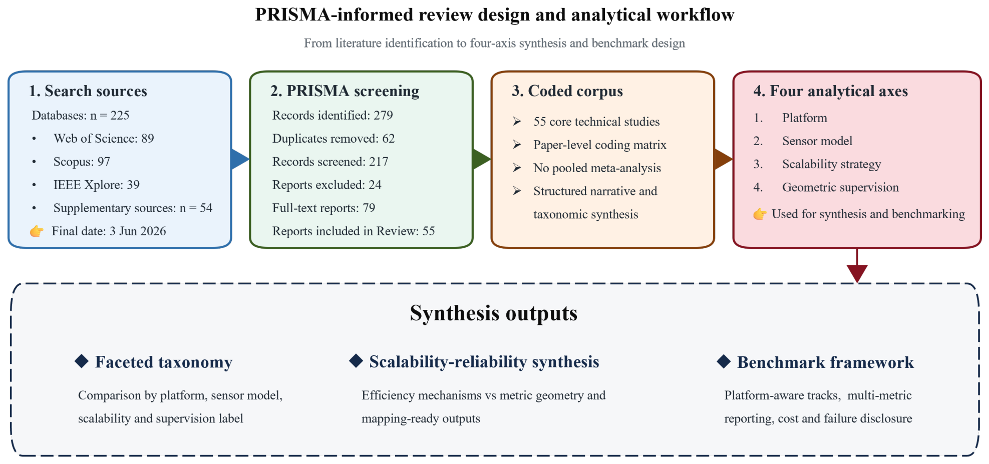
Web of Science, Scopus, and IEEE Xplore were searched and reconciled with prior Google Scholar screening, manuscript seed references, arXiv/publisher checks, and backward/forward citation chasing. The final search and corpus-reconciliation date was 3 June 2026. Search families combined 3DGS terms with remote sensing, UAV/aerial, satellite, scalability, geometry, and benchmark terms; Supplementary Table S2 records source-specific queries, dates, filters, and counts. Figure 2 links search, screening, coding, and synthesis.

Figure 2. Overview of the PRISMA-informed review design and analytical workflow. The schematic complements the PRISMA flow diagram by showing how record screening, paper-level coding, and the four analytical axes lead to the taxonomy and benchmark framework.

2.4. Eligibility Criteria

Core studies had to present a 3DGS method, substantive adaptation, or directly relevant radiance-field antecedent for large-scene or optical UAV/satellite reconstruction and provide enough methodological or evaluation detail for coding. Secondary reviews, standards, imagery/software sources, non-optical modalities, and application records without relevant method or evaluation evidence were excluded from the core corpus; boundary records were retained only as context. Supplementary Table S2 documents decisions and exclusion codes.

2.5. Study Selection Process

Records were merged and deduplicated by DOI and normalized title, screened by title/abstract, and assessed at full text. The first author performed initial screening and coding; borderline cases were checked with coauthors and the corresponding author. No automation tool excluded records. The pre-PRISMA draft contained 43 seed studies; database retrieval and reconciliation added 12 eligible studies, yielding the final 55-study corpus used throughout the manuscript and Supplementary Table S1 [19,20,21,22,23,24,25,26,27,32,33,34].

2.6. Study Selection Results

The search identified 279 records (225 database and 54 supplementary records). After removing 62 duplicates, 217 records were screened, 138 excluded, and 79 full texts assessed. Twenty-four were excluded, leaving 55 core studies (Figure 1).

2.7. Data Extraction and Coding

Supplementary Table S1 records citation metadata, corpus role, platform, sensor model, scene extent, initialization, priors, camera handling, representation, scalability strategy, geometric supervision, supervision class, target product, visual/geometry/cost metrics, benchmark relevance, limitations, and code/project availability. The first author applied a predefined matrix; ambiguous entries were checked against source papers and discussed with coauthors. The two principal evaluation lenses are rendering efficiency (time, memory, storage, Gaussian count, compression, and scale) and geometric reliability (height error, surface consistency, completeness, geo-alignment, orthophoto validity, and failures).

2.8. Synthesis Strategy

Heterogeneous platforms, sensors, scenes, supervision, metrics, and outputs precluded meta-analysis. We therefore used a narrative and thematic synthesis organized by platform, sensor model, scalability strategy, and geometric supervision. Original quantitative results are reported descriptively within their dataset and protocol rather than pooled.

2.9. Risk of Bias, Certainty Assessment, and Review Limitations

No intervention-style risk-of-bias or certainty tool was applied to this computational corpus; interpretability was instead assessed through sensor/model disclosure, supervision, metrics, costs, code/data availability, and reported limitations. Important limitations are rapidly changing preprints, less reproducible Google Scholar/citation chasing, heterogeneous protocols, and the absence of a shared executable benchmark. Preprint claims are therefore phrased as author-reported, and the benchmark is demonstrated with published scorecard entries rather than rerun experiments.

2.10. Protocol Registration

The review was not prospectively registered and no separate protocol was prepared. The questions, eligibility criteria, search, screening, coding, synthesis, and corpus-update procedure are documented here and in the Supplementary Materials.

3. Technical Background: From Photogrammetry and NeRF to 3DGS in Remote Sensing

In this section, we provide concise technical background needed for the rest of the review. Our goal is not to trace the full history of photogrammetry, NeRF, or Gaussian-based rendering. Instead, we briefly establish the common geometric language behind these methods and clarify why 3DGS became attractive for remote sensing, while also explaining why its vanilla formulation is insufficient for large-scale UAV and satellite scenarios.

3.1. Classical Photogrammetry Pipelines

Classical photogrammetry reconstructs scene geometry from multi-view image measurements by combining a sensor model, camera orientation, multi-view correspondence, and geometric optimization. In the most common ideal pinhole camera case, the image formation process can be written as

$$\lambda \left[\begin{array}{c}u\\ v\\ 1\end{array}\right]=\mathbf{K}\left[\begin{array}{cc}\mathbf{R}& \mathbf{t}\end{array}\right]\left[\begin{array}{c}X\\ Y\\ Z\\ 1\end{array}\right],$$

(1)

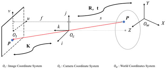
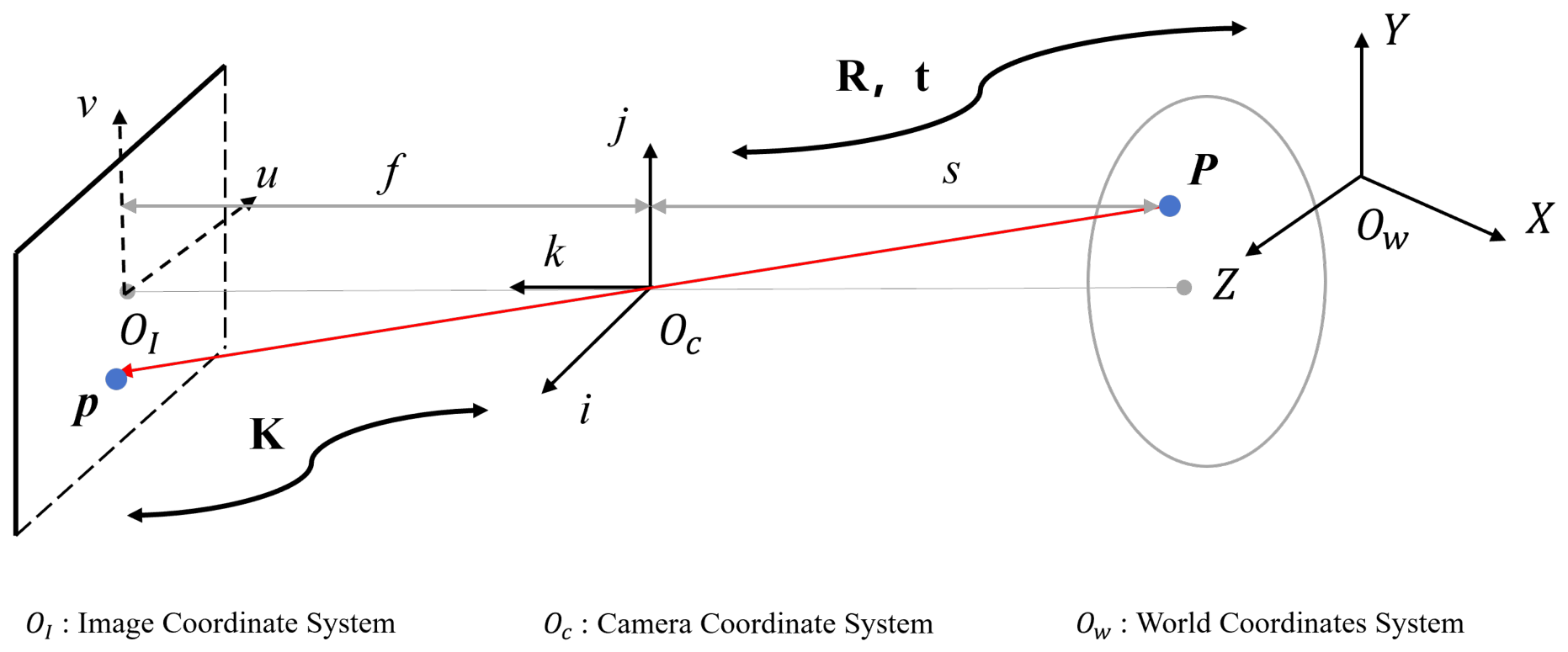
where $\lambda$ is a homogeneous scale factor; ${(X,Y,Z)}^{\top }$ denotes a 3D point in the world coordinate system, written here in homogeneous form as ${(X,Y,Z,1)}^{\top }$; ${(u,v)}^{\top }$ denotes the corresponding image coordinate, written in homogeneous form as ${(u,v,1)}^{\top }$; $\mathbf{K}$ is the intrinsic matrix; and $(\mathbf{R},\mathbf{t})$ are the extrinsic parameters. Figure 3 illustrates the coordinate transformation under the ideal pinhole camera model.

Figure 3. The most common ideal pinhole camera model.

In practice, this projection model is usually embedded in a broader reconstruction pipeline that includes image orientation, bundle adjustment, dense matching, and surface generation.

For remote sensing, however, the projection operator is not always well represented by a simple pinhole model. UAV imagery may require distortion-aware frame-camera calibration, whereas commercial optical satellite imagery may originate from a rigorous sensor model (RSM), be distributed with rational polynomial coefficients (RPCs), or be converted into a local affine or refined approximate camera model for efficient optimization [2,9,10]. It is therefore convenient to write image formation in a unified form as

$$\mathbf{p}={\Pi }_{\mathit{\theta }}\left(\mathbf{X}\right),$$

(2)

where ${\Pi }_{\mathit{\theta }}(·)$ denotes a sensor-dependent projection function parameterized by camera, orbit, line-array, RPC, or local-approximation parameters $\mathit{\theta }$. This compact notation is useful in the present review because later methods differ less in the existence of geometry than in how they model ${\Pi }_{\mathit{\theta }}$, refine $\mathit{\theta }$, and exploit auxiliary constraints such as LiDAR, relative heights, or georeferencing [6,17].

For satellite imagery, the projection chain should be interpreted more explicitly. Commercial high-resolution satellite images may be generated from a rigorous push-broom or line-array sensor model, in which image formation is line-dependent rather than frame-based. If $\mathbf{X}={(X,Y,Z)}^{\top }$ is an object-space point and $\mathbf{x}={(\mathsf{\ell },s)}^{\top }$ is the corresponding line–sample image coordinate, a simplified line-dependent model can be written as

$$t_{\mathsf{\ell }}=t_0+\mathsf{\ell }\Delta t,\hspace{1em}\mathbf{x}={(\mathsf{\ell },s)}^{\top }={\Pi }_{\mathrm{RSM}}\left(\mathbf{X};{\mathit{\theta }}_{\mathrm{RSM}}\left(t_{\mathsf{\ell }}\right)\right),$$

(3)

where $t_{\mathsf{\ell }}$ is the imaging time of line ℓ and ${\mathit{\theta }}_{\mathrm{RSM}}$ denotes time-dependent orbit, attitude, interior-orientation, and calibration parameters. This notation emphasizes that along-track and cross-track effects can be absorbed incorrectly when satellite images are treated as ordinary perspective frames.

In many practical satellite photogrammetry workflows, the physical sensor model is exposed to users through rational polynomial coefficients (RPCs). After normalizing object-space coordinates to $(X_n,Y_n,Z_n)$, the RPC mapping is commonly expressed as

$${\mathsf{\ell }}_n={\displaystyle \frac{P_{\mathsf{\ell }}(X_n,Y_n,Z_n)}{Q_{\mathsf{\ell }}(X_n,Y_n,Z_n)}},\hspace{1em}{s}_n={\displaystyle \frac{P_s(X_n,Y_n,Z_n)}{Q_s(X_n,Y_n,Z_n)}},$$

(4)

where $P_{\mathsf{\ell }},Q_{\mathsf{\ell }},P_s,Q_s$ are polynomial functions and $({\mathsf{\ell }}_n,s_n)$ are normalized line–sample coordinates. The pixel coordinates $(\mathsf{\ell },s)$ are then obtained through the corresponding image offset and scale parameters. Thus, RPC use in satellite 3DGS should be understood as a compact photogrammetric interface to the satellite image geometry, not as a rejection of rigorous sensor modeling.

Existing satellite 3DGS pipelines usually make this projection compatible with differentiable Gaussian optimization through RPC evaluation, RPC correction, or local affine approximation. At the review level, these choices can be summarized as

$${\Pi }_{\mathrm{ref}}\left(\mathbf{X}\right)={\mathbf{A}}_{\mathrm{img}} {\Pi }_{\mathrm{RPC}}\left({\mathbf{T}}_{\mathrm{obj}}\mathbf{X}\right)+{\mathbf{b}}_{\mathrm{img}},$$

(5)

or, within a bounded tile and height range, by the first-order local approximation

$$\Delta \mathbf{x}\approx {\mathbf{J}}_{\Pi }\left({\mathbf{X}}_0\right)\Delta \mathbf{X},\hspace{1em}{\mathbf{J}}_{\Pi }\left({\mathbf{X}}_0\right)={\left.{\displaystyle \frac{\partial \Pi }{\partial \mathbf{X}}}\right|}_{{\mathbf{X}}_0}.$$

(6)

Here, ${\mathbf{A}}_{\mathrm{img}}$ and ${\mathbf{b}}_{\mathrm{img}}$ denote image-space affine correction terms, ${\mathbf{T}}_{\mathrm{obj}}$ denotes an object-space normalization or transformation, and ${\mathbf{J}}_{\Pi }$ is the projection Jacobian evaluated around a local expansion point ${\mathbf{X}}_0$. These equations do not prescribe a single satellite 3DGS implementation. Rather, they identify the information that should be disclosed when reporting such methods: the projection interface, approximation domain, valid height range, refined variables, and whether the cost of camera/RPC refinement is included in the total runtime.

The limitations of these approximations should also be explicit. RPCs are compact approximations to the physical imaging model and should be used within their stated image extent, normalized-coordinate range, and height domain; residual biases may still require refinement. Local affine cameras are more restrictive because they are first-order approximations around a tile, an expansion point, and an assumed elevation range [6,16]. Their error can increase with tile footprint, off-nadir angle, terrain relief, sensor attitude variation, and distance from the local linearization point. In large-scale high-relief areas such as mountainous regions, a single affine approximation may absorb unmodeled push-broom and terrain-dependent effects as apparent surface deformation, leading to biased DSMs, warped geo-alignment, or block-boundary distortions. Satellite 3DGS papers should therefore report tile size, relief range, height interval, expansion point or linearization strategy, RPC-refinement residuals, and whether high-relief scenes are handled by smaller tiles, direct RPC evaluation, higher-order correction, or a more rigorous sensor model.

3.2. NeRF for Remote Sensing: Strengths and Bottlenecks

NeRF maps 3D position and viewing direction to density and color and renders images through volumetric ray integration [7]. NeRF++, Mip-NeRF 360, S-NeRF, Sat-NeRF, and EO-NeRF extended this formulation to unbounded scenes, scale-aware sampling, shadows, transient objects, multi-date appearance, and RPC-compatible satellite cameras [8,9,10,35,36]. These methods demonstrate the main strengths of radiance fields for remote sensing: continuous scene representation, view-dependent appearance modeling, and joint optimization of radiometry and scene structure. Their repeated field queries and dense ray sampling, however, remain costly for large, sparse-view, or multi-date collections, while photometric supervision alone provides limited control over DSMs, absolute heights, and geo-alignment [10,16,37].

Sensor and reflectance effects have therefore motivated more specialized radiance-field designs. Although not developed specifically for remote sensing, RS-NeRF models rolling-shutter image formation and jointly optimizes row-dependent camera motion, making it transfer-relevant to aerial or UAV frame imagery affected by line-wise readout distortion [38]. SatensoRF replaces repeated hierarchical MLP evaluation with a multiscale tensor decomposition for large multi-date satellite images, reducing parameter count and computation while modeling non-Lambertian appearance and temporal inconsistency [39]. BRDF-NeRF further incorporates the physically motivated semi-empirical Rahman–Pinty–Verstraete reflectance model, guided volumetric sampling, and depth supervision to handle sparse optical satellite views and changing illumination [40]. These developments improve sensor and appearance compatibility, but they do not remove the core bottlenecks of volumetric integration, scene-specific optimization, metadata sensitivity, and weak guarantees for metric products.

The transition from implicit fields to explicit Gaussians reduces repeated neural-field queries but introduces different representation and rasterization constraints. Mip-Splatting addresses scale-dependent aliasing through a 3D smoothing filter and a 2D Mip filter [41]; StopThePop improves view consistency through hierarchical re-sorting and culling of projected splats [42]; and Compact 3D Gaussian Representation reduces Gaussian count and attribute storage through learnable masking, neural color encoding, and vector quantization [43]. Together, these works show that replacing NeRF with 3DGS shifts, rather than eliminates, the main bottlenecks—from dense ray sampling toward aliasing, visibility ordering, and memory/storage—which motivates the explicit 3DGS formulation discussed next.

3.3. Original 3DGS: Explicit Gaussians and Differentiable Rasterization

3DGS replaces implicit per-sample field evaluation with an explicit set of learnable Gaussian primitives [1]. Each Gaussian is associated with a 3D mean ${\mu }_k$, an opacity $o_k$, an anisotropic covariance matrix ${\Sigma }_k$, and view-dependent appearance parameters, typically represented by spherical harmonics. A Gaussian kernel centered at ${\mu }_k$ can be written as

$$G_k\left(\mathbf{x}\right)=exp \left(-{\displaystyle \frac{1}{2}}{(\mathbf{x}-{\mu }_k)}^{\top }{\Sigma }_k^{-1}(\mathbf{x}-{\mu }_k)\right).$$

(7)

To ensure that ${\Sigma }_k$ remains positive definite during optimization, it is commonly parameterized through rotation and scaling as

$${\Sigma }_k={\mathbf{R}}_k {\mathbf{S}}_k{\mathbf{S}}_k^{\top } {\mathbf{R}}_k^{\top },$$

(8)

where ${\mathbf{R}}_k$ is a rotation matrix and ${\mathbf{S}}_k$ is a diagonal scaling matrix [1].

For rendering, the 3D Gaussian is projected into the image plane using a local affine approximation of the camera transform. If $\mathbf{W}$ denotes the world-to-camera linear transform and $\mathbf{J}$ the Jacobian of the projective mapping around the Gaussian center, the projected covariance can be written as

$${\Sigma }_k^{2D}=\mathbf{J} \mathbf{W} {\Sigma }_k {\mathbf{W}}^{\top }{\mathbf{J}}^{\top },$$

(9)

Here, the depth dimension is omitted after local linearization, so ${\Sigma }_k^{2D}$ denotes the $2\times 2$ image-plane covariance used for rasterization. After reducing the local covariance to the image-plane dimensions [1], the contribution of the k-th Gaussian to a pixel $\mathbf{p}$ is then modeled by a screen-space opacity

$${\alpha }_k\left(\mathbf{p}\right)=o_{k}exp\left(-{\displaystyle \frac{1}{2}}{(\mathbf{p}-{\mu }_k^{2D})}^{\top }{\left({\Sigma }_k^{2D}\right)}^{-1}(\mathbf{p}-{\mu }_k^{2D})\right),$$

(10)

and final rendering is obtained by front-to-back alpha compositing:

$$\widehat{\mathbf{I}}\left(\mathbf{p}\right)={\displaystyle \sum _{k=1}^K}{T}_k\left(\mathbf{p}\right){\alpha }_k\left(\mathbf{p}\right){\mathbf{c}}_k,\hspace{1em}{T}_k\left(\mathbf{p}\right)=\prod _{j<k}\left(1-{\alpha }_j\left(\mathbf{p}\right)\right),$$

(11)

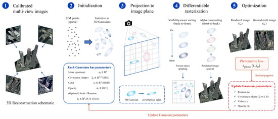
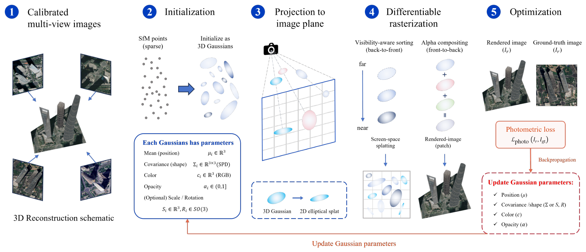
where the Gaussians are depth-sorted before splatting. Figure 4 summarizes the standard pipeline of the original 3DGS method.

Figure 4. The standard pipeline of original 3DGS method.

Compared with NeRF, 3DGS stores geometry and appearance in explicit rasterizable primitives, which enables rapid rendering and adaptive densification from sparse Structure-from-Motion (SfM) initialization [1,29]. The same volumetric flexibility weakens surface guarantees in poorly observed areas. 2D Gaussian Splatting (2DGS) addresses this with surface-oriented splats and depth/normal regularization, while CityGaussianV2 couples large-scene efficiency with stronger geometry [13,44].

3.4. Why Remote Sensing Is Different

Generic 3DGS benchmarks usually assume perspective cameras, dense coverage, bounded scenes, and image-space evaluation. Remote sensing adds distortion-aware UAV cameras, push-broom/RPC satellite geometry, weak or anisotropic parallax, multi-date radiometry, large spatial extent, geodetic coordinates, and mapping products. Consequently, remote-sensing methods must address sensor consistency, scalable optimization, geometric supervision, and product-level validation rather than NVS alone [2,3,6,16,17].

4. Taxonomy of 3DGS for Large-Scale Remote Sensing

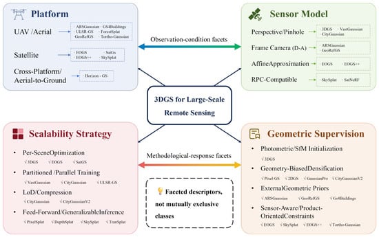
Chronology alone does not explain why large-scale 3DGS methods differ. We therefore use a faceted taxonomy with four descriptors: platform, sensor model, scalability strategy, and geometric supervision. Platform and sensor models describe observation conditions; scalability and supervision describe methodological responses. The axes may correlate and are not mutually exclusive. Figure 5 summarizes this structure.

Figure 5. A faceted four-axis taxonomy for 3D Gaussian splatting in large-scale remote sensing. The platform and sensor-model axes describe observation conditions, while the scalability and geometric-supervision axes describe methodological responses. The axes are comparability descriptors rather than mutually exclusive or statistically independent classes.

4.1. Platform Axis: UAV, Satellite, and Cross-Platform Settings

UAV/aerial methods often exploit perspective or distortion-aware cameras, SfM/LiDAR support, GCPs, georeferencing, structural priors, or orthophoto supervision [2,3,4,5,15,24,25,26,27,45]. Satellite methods face long stand-off distance, weak parallax, push-broom/RPC geometry, shadows, and temporal change, motivating affine/RPC modeling, camera refinement, uncertainty, and height-product evaluation [6,9,16,17,18,19,20,21,22,23]. Hybrid methods such as Horizon-GS address cross-altitude integration [46].

4.2. Sensor-Model Axis: From Perspective Cameras to RPC-Compatible Splatting

Generic 3DGS assumes calibrated perspective cameras; remote sensing may require UAV distortion models, pose/georeferencing refinement, LiDAR alignment, or satellite-specific projection [1,2,3,47]. Sat-NeRF, EOGS, EOGS++, and SkySplat span RPC-aware rendering, local affine approximation, internal refinement, and RPC-compatible generalization [6,9,16,17]. Comparisons must disclose projection interface, tile and height domain, terrain relief, refined variables, and residual checks because RPC/affine validity differs between compact low-relief tiles and wide mountainous areas.

4.3. Scalability Axis: Per-Scene Optimization, Partitioning, LoD, and Generalization

Scalability strategies include per-scene optimization, partitioned/parallel training, LoD or hierarchy, pruning/compression, and feed-forward generalization. VastGaussian, CityGaussian, CityGaussianV2, hierarchical 3DGS, Momentum-GS, LightGaussian, Compressed 3DGS, and generalizable pipelines illustrate these choices [11,12,13,14,48,49,50,51,52,53,54]. Their gains must be interpreted against seams, storage, training/pretraining costs, geometry retention, and adaptation requirements.

4.4. Geometric-Supervision Axis: From Photometric Consistency to Mapping-Ready Constraints

Supervision ranges from image-only photometric consistency and internal camera refinement to sparse georeferencing, dense LiDAR/DSM/depth support, semantic or structural priors, and amortized pretraining. Surface-aware methods such as 2DGS, Pixel-GS, SuGaR, Gaussian Surfels, and GaussianPro improve geometric regularity, while ARSGaussian, GeoRefGS, GS4Buildings, EOGS++, GU-GS, and product-oriented methods tie reconstruction to remote-sensing geometry or outputs [2,3,5,17,21,44,45,55,56,57,58]. Supervision labels are therefore required for fair comparison.

4.5. Mapping Representative Methods to the Taxonomy

Table 1 maps representative methods to the four axes. The table is not intended as an exhaustive leaderboard or a set of mutually exclusive classes. It is a structured reading guide for a faceted taxonomy. Our purpose is to show how methods that share the label “Gaussian splatting” differ in platform assumptions, sensor handling, scalability mechanisms, and geometric commitments.

Table 1. Representative methods mapped to the proposed taxonomy. The entries summarize the primary role of each method rather than all implementation details.

Method	Platform	Sensor Model	Scalability Strategy	Geometric Supervision/Taxonomy Role
3DGS [1]	Generic scenes	Perspective cameras	Per-scene optimization	Establishes explicit Gaussian representation and differentiable rasterization; weak surface guarantees under remote-sensing conditions.
VastGaussian [11]	Generic large scenes	Perspective cameras	Partitioned and parallel training	Provides a core large-scene scaling paradigm, but with limited remote-sensing-specific sensor or geometric modeling.
CityGaussian [12]	Generic city-scale scenes	Perspective cameras	Divide-and-conquer training with LoD rendering	Strong reference for real-time large-scene rendering; geometry is improved mainly through large-scene organization rather than explicit remote-sensing constraints.
CityGaussianV2 [13]	Generic large scenes	Perspective cameras	Parallel training, compression, and geometry-aware design	Important bridge between efficiency and geometric accuracy; relevant to remote sensing but not sensor-specific.
ULSR-GS [15]	UAV/aerial urban scenes	Perspective cameras	Point-to-photo partitioning	Surface-oriented reconstruction with multi-view geometric consistency; useful comparator for geometry-focused remote-sensing 3DGS.
ARSGaussian [2]	UAV/aerial remote sensing	Distortion-aware frame cameras with LiDAR alignment	Per-scene optimization	Uses LiDAR-guided densification and geometric constraints to suppress floaters and improve metric reconstruction.
EOGS [16]	Satellite imagery	RPC approximated by affine cameras	Per-scene optimization	Adapts Gaussian splatting to satellite photogrammetry with satellite-aware projection and altitude-related regularization.
EOGS++ [17]	Satellite imagery	Affine satellite cameras with internal refinement	Per-scene optimization	Strengthens satellite 3DGS through camera refinement, panchromatic rendering, and geometry-oriented post-processing.
SatGS [18]	Multi-temporal satellite imagery	Satellite-oriented image geometry	Per-scene optimization	Emphasizes appearance-adaptive reconstruction under temporal variation; useful for radiometric and seasonal robustness.
SkySplat [6]	Sparse multi-temporal satellite imagery	RPC-compatible modeling	Generalizable feed-forward reconstruction	Key representative of satellite generalizable 3DGS with relative-height supervision and consistency masking.
GeoRefGS [3]	UAV geospatial applications	Perspective cameras with georeferenced transformation	Per-scene optimization	Introduces geographic constraints into training; important for mapping-ready Gaussian representations.
GS4Buildings [45]	UAV urban buildings	Camera parameters with LoD2 building priors	Prior-guided per-scene optimization	Converts structured building priors into depth and normal constraints for more complete building reconstruction.
ForestSplat [4]	UAV forestry mapping	UAV frame imagery	Scalable scene reconstruction	Demonstrates product-oriented use of 3DGS for forestry mapping rather than view synthesis alone.
Tortho-Gaussian [5]	UAV/aerial orthophoto production	Perspective input with orthographic product generation	Task-oriented Gaussian splatting	Uses Gaussian representations for true digital orthophoto production; highlights product-level geometric requirements.
Horizon-GS [46]	Aerial-to-ground hybrid scenes	Mixed perspective views	Unified cross-view large-scene reconstruction	Explores cross-altitude fusion; relevant to digital twins, though less focused on strict geospatial products.
PixelSplat, TranSplat, DepthSplat [52,53,54]	Generic sparse-view scenes	Perspective cameras	Feed-forward generalization	Provide transferable mechanisms for sparse-view Gaussian prediction, depth-aware inference, and generalizable reconstruction.

The mapping reveals a persistent imbalance: generic large-scene methods are mature in efficiency, whereas remote-sensing methods remain dominated by per-scene optimization and platform-specific priors. UAV methods provide the strongest external geometry, and satellite methods emphasize RPC/affine cameras, temporal robustness, and height recovery. Separating scalability from supervision therefore prevents rendering gains from being mistaken for metric reliability [2,6,11,12,13,15,16,17,18].

5. Scalability and Rendering Efficiency in Large-Scale Remote Sensing

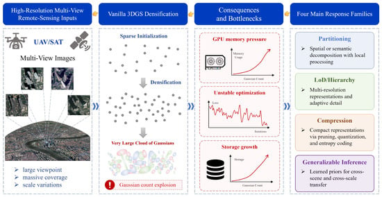
This section treats scalability as an end-to-end property rather than a frame-rate number. For large-scale remote sensing, efficiency includes preprocessing, partitioning, optimization, storage, rendering, product extraction, and the ability to keep geometry reliable as scene extent, image count, and Gaussian count grow [1,6,11,12,13,16,29]. Figure 6 summarizes the main bottlenecks and representative optimization strategies.

Figure 6. Vanilla 3DGS’s bottlenecks and subsequent optimization methods.

5.1. Scaling Bottlenecks

Vanilla 3DGS remains a per-scene optimizer. This is effective for bounded scenes, but large UAV blocks and multi-temporal satellite collections increase Gaussian count, optimizer state, visibility buffers, memory use, and gradient imbalance. A single global Gaussian pool can overfit well-observed regions while leaving weakly constrained roofs, terrain, vegetation, or low-parallax satellite areas unstable [1,11,12]. Remote-sensing products also impose a stronger requirement than view synthesis: a fast renderer is not operationally useful if block seams, weak georeferencing, or unstable height surfaces prevent DSM, orthophoto, mesh, or georeferenced-scene generation [3,5,16,17].

5.2. Efficiency Strategies

Current scaling strategies fall into four groups. Per-scene optimization, used by vanilla 3DGS and many early remote-sensing adaptations, is flexible but costly for repeated scenes [1,16,18]. Partitioned and parallel methods such as VastGaussian, CityGaussian, CityGaussianV2, ULSR-GS, and UAV-specific partitioning approaches reduce memory and training burden but must control seams, cross-block consistency, and partition-dependent density drift [11,12,13,15,32,33]. LoD, compression, pruning, and storage-aware representations reduce deployment cost but can remove fine structures needed for roofs, façades, terrain discontinuities, or product boundaries [12,13,25,34,50,51]. Feed-forward or generalizable pipelines such as pixelSplat, TranSplat, DepthSplat, AnySplat, SkySplat, and SatSurfGS reduce per-scene optimization, but their geometric reliability under sensor heterogeneity, seasonal change, and large geographic extent remains an open evaluation issue [6,14,22,52,53,54].

5.3. Operational Definition

For benchmark use, scalability should be reported as a vector rather than a single score: preprocessing time, training or adaptation time, rendering speed, product-generation time, peak memory, model size, Gaussian count, storage, partition overhead, and geometry retained after scaling or compression. A method that renders quickly but requires heavy manual preprocessing or loses height fidelity is not necessarily more scalable for remote-sensing use. This motivates the next section, which treats metric reliability as a co-equal requirement.

6. Geometric Constraints and Metric Reliability

Remote sensing requires 3DGS to retain metrically stable structure for DSMs, orthophotos, buildings, vegetation, and georeferenced scenes, not merely fast rendering [1].

6.1. Failure Modes Without Explicit Geometry

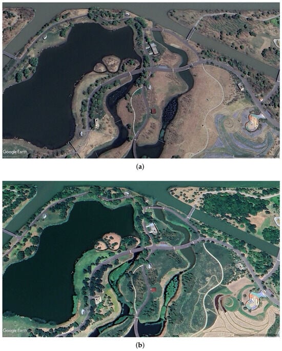
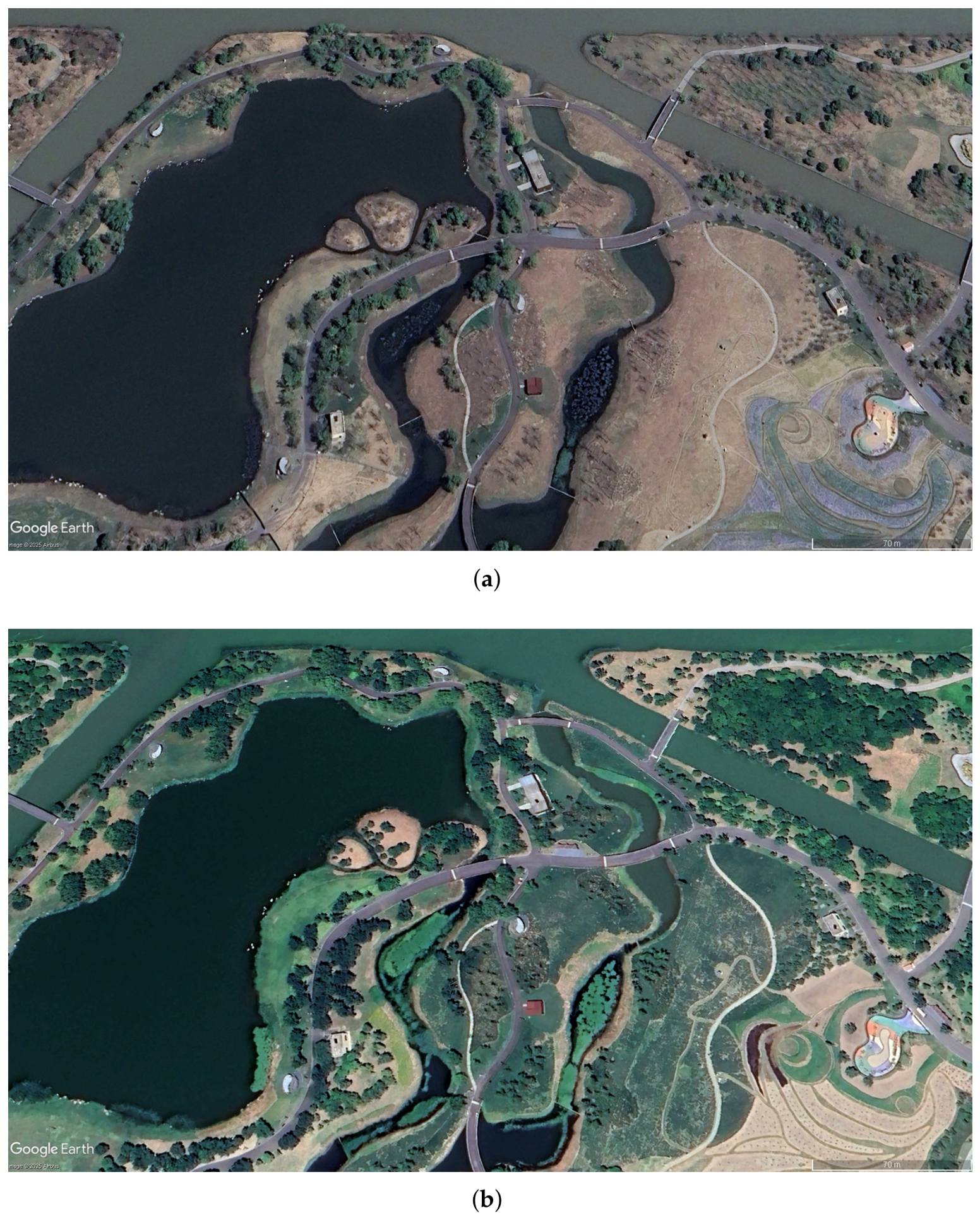
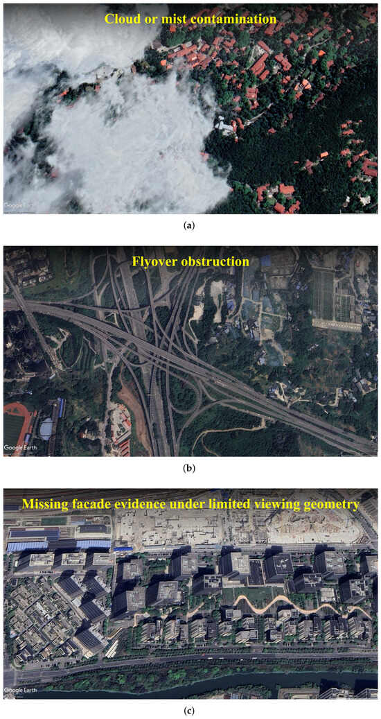
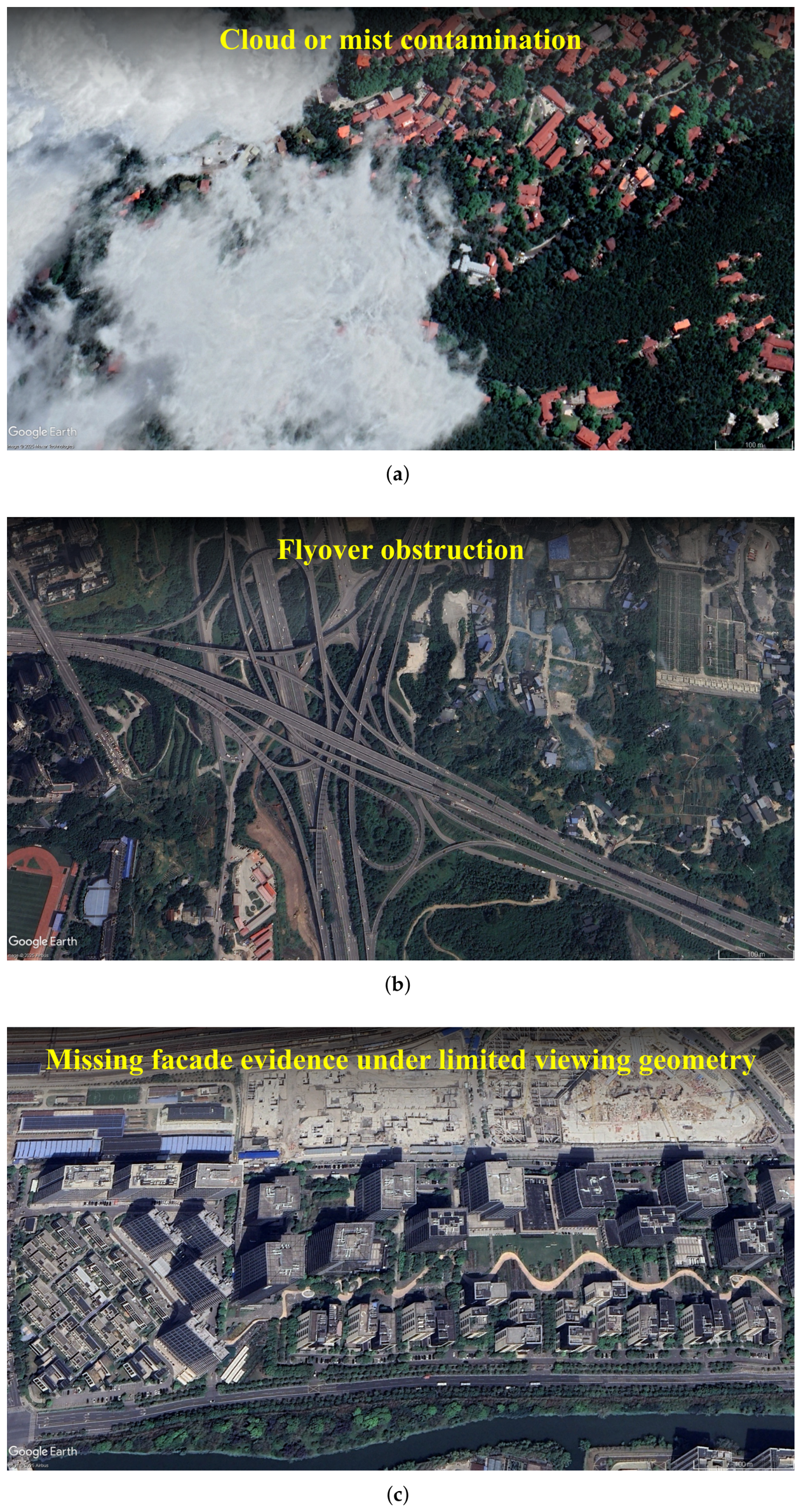
Weakly constrained 3DGS can improve photometric fit while producing floaters, elongated splats, doubled surfaces, blurred boundaries, unstable thin structures, or depth bleeding. In remote sensing these artifacts are not cosmetic: they can become height errors, roof-edge distortion, orthophoto artifacts, or invalid DSM products. The problem is amplified by sparse or anisotropic views, weak satellite parallax, shadows, multi-date appearance changes, and imperfect camera or RPC models [6,8,9,10,16]. Figure 7 and Figure 8 are qualitative illustrations only; they motivate why photometric-only optimization can fail under temporal change, contamination, occlusion, and missing façade evidence.

Figure 7. An illustrative example of significant temporal variation in multi-date remote-sensing imagery over Shanghai Binjiang Forest Park, Shanghai, China: (a) observation in April 2025, showing comparatively sparse vegetation and more exposed ground surfaces; (b) observation in July 2024, showing denser vegetation cover over the same area. Imagery © 2025 Airbus, accessed via Google Earth Pro on 26 May 2026, and shown here for qualitative illustration only [59].

Figure 8. Illustrative causes of information loss in satellite reconstruction. (a) Cloud or mist contamination. (b) Flyover obstruction. (c) Missing facade evidence under limited viewing geometry. Imagery © 2025 Airbus and Maxar Technologies, accessed via Google Earth Pro on 26 May 2026, and shown here for qualitative illustration only [59].

A methodological consequence is that photometric supervision alone is underdetermined: many 3D configurations can yield similar image-space fidelity under sparse or biased viewing. The most relevant innovations for remote sensing are therefore not just those that improve PSNR, but those that inject, preserve, or evaluate geometry while remaining compatible with efficient Gaussian rendering [2,17,44,45].

6.2. Control-Point-Free and Weakly Supervised Metric Reliability

LiDAR, GCPs, and dense reference DSMs are not always available. In control-point-free satellite or wide-area settings, absolute metric accuracy cannot be certified as an externally validated product, but reliability can still be improved and partially audited through sensor-consistent projection, image-only camera/RPC refinement, multi-view reprojection consistency, epipolar or height-range constraints, surface or normal-depth regularity, temporal/shadow masking, uncertainty estimation, and held-out-view or held-out-date validation. These internal checks should be reported as consistency evidence, not as independent DSM or geo-alignment accuracy; the benchmark framework therefore separates supervision class, reference-data availability, internal consistency, and externally validated product metrics.

6.3. UAV and Airborne Branch: LiDAR Fusion, Alignment, and Regularization

UAV methods provide the clearest geometry-aware examples. ARSGaussian combines LiDAR-guided densification, alignment, geometric consistency, and bundle adjustment; GeoRefGS learns a georeferenced transformation; ULSR-GS, GS4Buildings, and Tortho-Gaussian target surface consistency, structural priors, and true orthophotos [2,3,5,15,45]. Benchmarks must state whether LiDAR, GCPs, georeferencing, priors, or product references are used for training, alignment, post-processing, or evaluation.

6.4. Satellite Branch: RPC Cameras, Bundle Adjustment, and Temporal Robustness

Satellite 3DGS is geometrically demanding because long stand-off distance weakens convergence, push-broom geometry is line-dependent, RPC or affine approximations replace simple perspective cameras, and multi-date collections introduce shadows, seasonal change, and radiometric inconsistency. Sat-NeRF and EO-NeRF already showed that RPC modeling, shadow handling, transient-object treatment, bundle adjustment, and DSM recovery are central in satellite neural reconstruction [9,10]. Gaussian-based satellite methods inherit these constraints: EOGS uses local affine satellite projection, EOGS++ adds camera refinement and TSDF processing, and SatGS, SkySplat, ShadowGS, and SatSurfGS address temporal appearance, RPC-compatible generalization, shadow-aware supervision, and confidence-aware surface recovery [6,16,17,18,19,22].

The remaining limitation is that RPC and affine handling can themselves become a source of geometric error. RPC metadata may be biased or insufficiently refined, and local affine approximations are valid only over limited image tiles and height intervals. The risk is especially high in large mountainous or high-relief regions, where elevation varies rapidly within one tile and the first-order linearization no longer represents the true push-broom/RPC projection. In such cases, the optimizer may compensate for projection error by deforming Gaussian geometry, creating DSM bias, block seams, or geo-alignment distortion. Satellite 3DGS results should therefore report the approximation domain, terrain-relief range, height interval, camera/RPC refinement residuals, tile-size policy, and whether high-relief areas use smaller tiles, direct RPC evaluation, or a more rigorous sensor model.

6.5. Surface-Oriented and Prior-Guided Gaussian Variants

2DGS, SuGaR, and Gaussian Surfels bias Gaussians toward surfaces through flattened primitives, mesh binding, or depth/normal consistency [44,56,57]. CityGaussianV2, GS4Buildings, and Tortho-Gaussian connect these ideas to large scenes, structural priors, and map products [5,13,45]. Because vegetation and clutter are not clean surfaces, future systems may need adaptive mixtures of surface-biased and volumetric primitives.

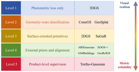
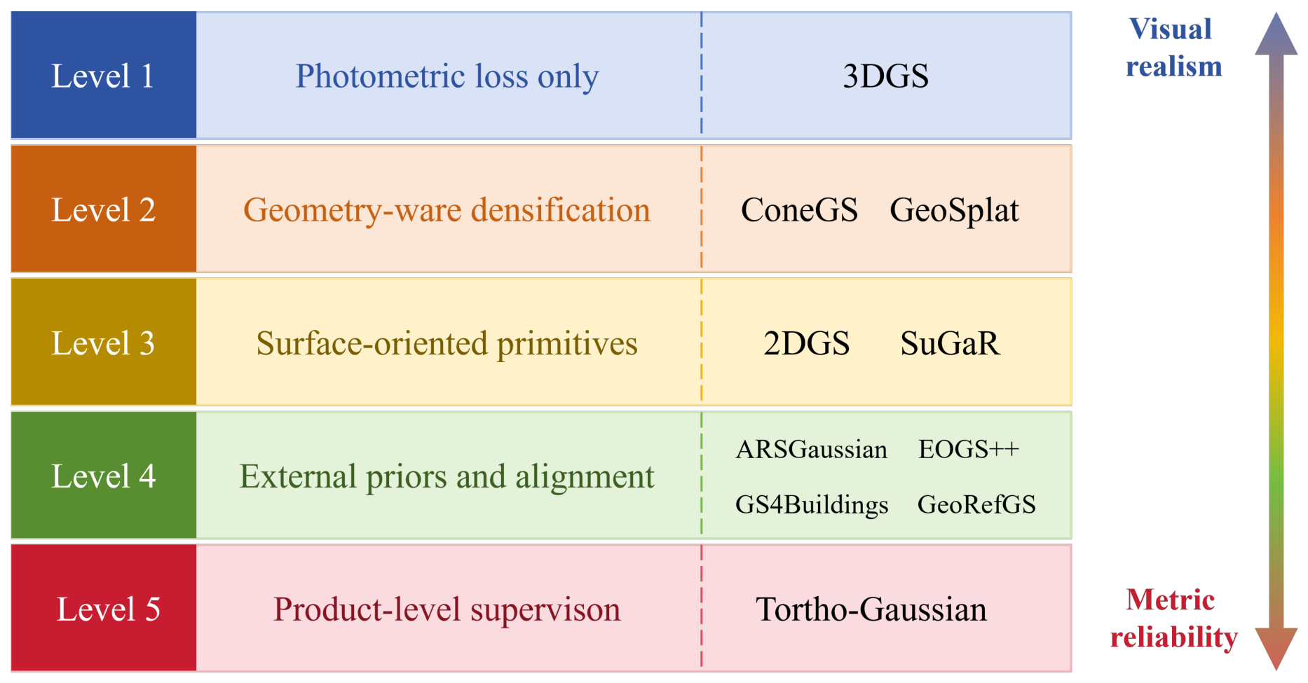
Figure 9 shows a supervision hierarchy from photometric realism to metric remote-sensing reliability.

Figure 9. A supervision hierarchy from photometric realism to metric remote-sensing reliability.

6.6. From Visual Realism to Measurable Geometry

Remote-sensing 3DGS should be evaluated at three levels: rendering fidelity (PSNR, SSIM, learned perceptual image patch similarity (LPIPS), and visual consistency), geometric reliability (DSM MAE/RMSE, point-to-surface distance, completeness, boundary precision, and height residuals), and geospatial utility (orthophoto production, building reconstruction, geo-registration, or mapping at the intended scale). EOGS/EOGS++, GeoRefGS, GS4Buildings, and Tortho-Gaussian are important because they foreground elevation recovery, geographic alignment, and product-oriented structural quality [3,5,16,17,45]. This reinforces the main thesis: the field must move from visually plausible reconstruction to sensor-aware, scalable, and metrically constrained scene representation.

7. Cross-Platform Synthesis and Benchmark Implications

UAV and satellite 3DGS share three requirements: scalable scene representation, sensor-consistent optimization, and product-level validity. Large-scene methods address Gaussian growth through partitioning, LoD, hierarchy, or compression [11,12,13,48]; remote-sensing methods additionally tie optimization to georeferencing, LiDAR, structural priors, orthophotos, or satellite cameras and height products [2,3,5,6,15,16,17,24,45].

The platforms nevertheless require separate tracks. UAV/aerial imagery usually provides stronger parallax and more external control, supporting LiDAR- or prior-assisted surface and product reconstruction [2,26,27]. Satellite imagery combines push-broom/RPC geometry, weaker baselines, temporal gaps, shadows, and atmospheric variation; SatGS, SkySplat, ShadowGS, SA-GS, GU-GS, SatSurfGS, and semantic-feature methods address appearance, generalization, uncertainty, and DSM recovery [6,18,19,20,21,22,23]. A common reporting core should therefore be paired with platform-specific evaluation.

7.1. Efficiency–Geometry Trade-Offs Across Method Families

Across method families, the core trade-off is scalability versus geometry retention under platform-specific sensing constraints. Partitioning, hierarchy, compression, surface-biased primitives, prior-guided supervision, and generalizable inference each improve one part of the pipeline while changing seam consistency, model size, supervision assumptions, height fidelity, or cost accounting [2,6,11,12,13,15,17,44,45,48,50,51,56,60]. A scientifically useful benchmark should therefore use a Pareto-style scorecard rather than a single aggregate score.

A full same-dataset leaderboard across UAV/aerial and satellite 3DGS is not currently defensible because the reviewed studies differ in scenes, sensor models, supervision regimes, outputs, and metric definitions. Table 2 therefore summarizes reported metric families and comparability limits rather than pooled performance. The shorthand S0–S5, defined formally in Section 8.3, denotes fixed-camera image-only, internally refined image-only, sparse-control/georeferenced, dense-geometry-assisted, semantic/structural-prior-guided, and amortized/generalizable supervision, respectively.

Table 2. Representative reported metrics and comparability limits across large-scale and remote-sensing 3DGS methods. Metric names are summarized at the review level; numerical values should be compared only within the same dataset, split, sensor model, and supervision class.

Representative Method	Track/Scene Type	Supervision Class	Visual Metrics Reported	Geometry/Product or Cost Metrics Reported	Direct-Comparison Caution
EOGS [16]	Satellite photogrammetry	S1	PSNR, SSIM, LPIPS	DSM/height error; training time; rendering speed	Comparable mainly with satellite methods using the same RPC/affine setup and DSM reference.
EOGS++ [17]	Satellite photogrammetry with camera refinement	S1	Image reconstruction metrics	DSM/height quality; panchromatic rendering; preprocessing/post-processing cost	Camera refinement and TSDF processing must be cost-accounted before comparing with image-only baselines.
SatGS [18]	Multi-temporal satellite NVS	S0/S1	PSNR, SSIM, LPIPS	Temporal robustness indicators; limited product geometry	Useful for appearance robustness, but not sufficient as a DSM benchmark without product metrics.
SkySplat [6]	Sparse multi-temporal satellite reconstruction	S5/S1	PSNR, SSIM, LPIPS	Height/depth-related metrics; inference speed; pretraining cost	Feed-forward cost structure is not directly comparable to per-scene optimization unless pretraining and adaptation are separated.
GU-GS [21] and SatSurfGS [22]	Satellite DSM/surface reconstruction	S1 or S5/S1	Image metrics as reported	DSM or surface accuracy; uncertainty or confidence indicators; speedup relative to selected baselines	Geometry comparison depends on reference DSM quality, valid mask, and whether the method is generalizable or per-scene.
ARSGaussian [2]	UAV/aerial LiDAR-assisted reconstruction	S3	PSNR, SSIM, LPIPS	LiDAR/geometry errors; depth, normal, and scale consistency; runtime/memory	Should not be ranked against S0 image-only methods without a separate LiDAR-assisted track.
GeoRefGS [3]	UAV georeferenced reconstruction	S2	Image metrics as applicable	Geo-alignment or positioning accuracy; optimization cost	Requires explicit coordinate reference system (CRS), transformation, and checkpoint disclosure.
Tortho-Gaussian and Ortho-3DGS [5,24]	UAV/aerial orthophoto products	S0/S1	Product/image quality indicators	True orthophoto artifacts, geometric accuracy, completeness, product-generation cost	Product metrics are task-specific and should not be reduced to held-out-view scores.
C3DGS for UAV and StitchGS [25,34]	Large-scale UAV or city-scale deployment	S0/S1	PSNR, SSIM, LPIPS as reported	Compression ratio, storage reduction, seam or boundary consistency, reconstruction detail	Compression gains must be interpreted together with geometry retention and partition-boundary quality.

Table 3 gives a small worked example of how the proposed scorecard can be populated from values reported by original UAV and satellite studies. The table is not a new experiment and does not claim statistical pooling. Its purpose is to demonstrate the benchmark logic: visual quality, DSM/height error, cost, supervision class, and sensor-model assumptions must be read together. For example, a method may report strong image quality in one area of interest while another method reports lower height error or much lower deployment time; the benchmark should expose such trade-offs instead of hiding them behind one aggregate rank.

Table 3. Worked scorecard example using reported UAV and satellite results from the original papers. Values are copied or summarized from the cited studies and should be interpreted only within their reported datasets, splits, masks, and evaluation protocols.

Method	Reported Setting	Supervision/ Sensor Label	Geometry or Product Scorecard Entry	Cost or Visual Scorecard Entry	Benchmark Interpretation
EOGS [16]	DFC2019 and IARPA2016 satellite AOIs, RPCs locally approximated as affine cameras	S1; satellite affine/RPC approximation	Elevation MAE reported by the authors: JAX mean 1.46 m and IARPA mean 1.62 m without foliage mask; JAX mean 1.19 m and IARPA mean 1.37 m with foliage mask.	Training time reported as about 3 min; approximately 300× faster than EO-NeRF in the reported setting.	A strong speed–height trade-off example; valid comparison requires declaring mask use, AOI coverage, affine approximation, and LiDAR/DSM reference.
GeoRefGS [3]	Unity-simulated UAV urban reconstruction with global-coordinate constraints	S2; UAV georeferencing/ geographic-loss supervision	Authors report a mean planar checkpoint error of 0.054 m for the full model in the simulated setting.	Authors report an approximately 3.31 dB PSNR improvement while maintaining georeferenced reconstruction accuracy.	UAV example showing that image fidelity and geographic accuracy should be reported together; coordinate-system handling, similarity transformation, checkpoint definition, and simulated-versus-real data status should be declared.
SkySplat [6]	DFC19 sparse multi-temporal satellite reconstruction; generalizable feed-forward inference	S5/S1; RPC-compatible generalizable satellite pipeline	Authors report MAE reduction from 13.18 m to 1.80 m against generalizable baselines on DFC19; reported cross-dataset tests use MVS3D.	Authors report 86× speedup over EOGS; in the per-scene comparison, reconstruction time is reduced from 4.60 min for EOGS to 3.19 s for SkySplat, with lower reported elevation MAE across the listed AOIs.	Shows why height metrics, deployment cost, supervision class, and sensor-model assumptions should be reported jointly; pretraining, inference, and per-scene adaptation costs should remain separated.

7.2. Implications for Benchmark Design

A credible benchmark must be platform-aware, report efficiency with geometry and product utility, and expose supervision and sensor assumptions. It should therefore use separate tracks, declared supervision classes, decomposed costs, multi-family metrics, and explicit failure reporting rather than a single pooled ranking.

8. Toward a Reproducible Benchmarking Framework

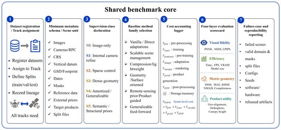
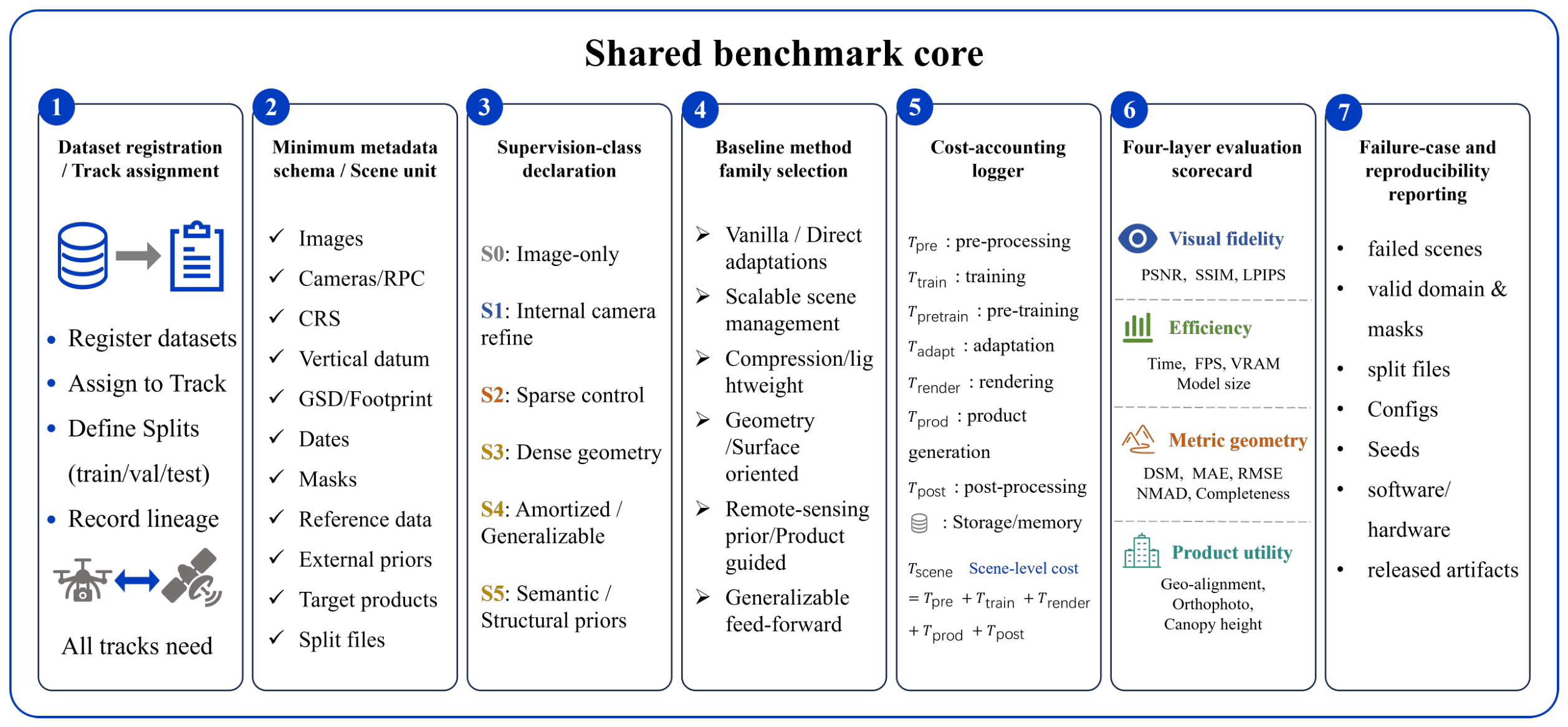
The synthesis above leads to one benchmark principle: large-scale remote-sensing 3DGS should be evaluated through a structured scorecard, not a generic NVS leaderboard. Performance must be interpreted jointly by platform track, sensor model, scalability strategy, supervision class, cost model, visual fidelity, metric geometry, product utility, and failure behavior [2,11,13]. Figure 10 summarizes the proposed framework.

Figure 10. Operational structure of the proposed reproducible benchmark framework for large-scale remote-sensing 3DGS.

8.1. Benchmark Objectives and Design Principles

A useful benchmark should make cross-paper comparison more defensible, expose efficiency–geometry trade-offs, and remain extensible. We therefore define it as dataset-agnostic but metadata-strict and track-based rather than method-centered: each scene must carry standard metadata, and methods should be compared first within declared task settings before any cross-track interpretation.

8.2. Dataset Tracks, Scene Units, and Minimum Metadata

The benchmark defines a scene unit by footprint, images, sensor model, coordinate reference, split, masks, and reference products; tiled areas additionally require boundaries, overlap, and aggregation rules. Four primary tracks are recommended: UAV image/NVS; UAV geometry-product; satellite RPC/multi-view; and satellite multi-temporal robustness, with hybrid UAV–satellite or aerial–ground data treated as exploratory. Direct comparison is restricted to the same track, split, sensor setting, and compatible supervision.

Each release should separate development and locked test scenes and publish, where licensing permits, scene identifiers, checksums, splits, masks, and versioned evaluation scripts. Minimum metadata include footprint, GSD, CRS and vertical datum, acquisition geometry, sensor/camera model, temporal record, preprocessing, reference data, priors, target products, and access restrictions. Satellite records additionally require an RPC source, an affine/refinement strategy, an approximation domain, a height interval, a terrain-relief range, and residual checks. Supplementary File S3 provides the machine-readable YAML schema.

8.3. Supervision Classes and Baseline Method Groups

Baseline grouping should distinguish method family from supervision class. Families describe algorithmic roles; supervision classes describe what information a method is allowed to use. Each experiment should report one or more classes from Table 4—for example, S2 + S3 for GCP + LiDAR supervision or S1 + S5 for pretrained prediction with per-scene RPC refinement. These are comparability labels, not quality levels.

Table 4. Supervision classes for fair comparison of remote-sensing 3DGS methods.

Class	Name	Allowed Information	Mandatory Disclosure
S0	Image-only with fixed initial cameras	Input images and provided initial cameras or RPCs; photometric losses; no external geometry, semantic labels, dense depth, GCPs, or pretrained external scenes.	Camera source; whether camera parameters are frozen; image preprocessing; initialization points if used.
S1	Image-only with internal camera refinement	S0 information plus camera, pose, affine, or RPC refinement using only the benchmark images.	Refinement variables; refinement schedule; whether refinement occurs before training or inside optimization; cost of refinement.
S2	Sparse-control or georeferenced supervision	S0/S1 information plus sparse GCPs, checkpoints, GNSS/IMU, georeferencing constraints, or sparse tie/control measurements.	Number, distribution, and accuracy of control points; whether control is used for training, alignment, or evaluation only.
S3	Dense-geometry-assisted supervision	S0/S1/S2 information plus LiDAR, reference DSM, depth maps, meshes, dense point clouds, normals, or height fields used during training or regularization.	Data source; density or resolution; vertical datum; quality level; registration method; whether reference data also appear in evaluation.
S4	Semantic or structural-prior-guided supervision	Building footprints, LoD2/LoD3 models, road masks, land-cover labels, object masks, planar priors, roof models, or other explicit structural priors.	Prior source; label accuracy; whether priors are used for masking, loss terms, initialization, pruning, or post-processing.
S5	Amortized or generalizable supervision	External training scenes, pretrained networks, foundation models, cross-scene feed-forward predictors, or meta-learned initializations.	Pretraining data; number and type of scenes; overlap with test geography; pretraining cost; per-scene adaptation policy.

Table 5 groups baseline families by benchmark role: vanilla/direct adaptations, scalable scene management, compression, geometry/surface variants, remote-sensing sensor/prior/product methods, and generalizable feed-forward pipelines. These families are not disjoint—for example, CityGaussianV2, EOGS++, and SkySplat combine multiple roles—but the grouping clarifies which capability is being tested, while supervision classes clarify whether the comparison is fair [6,13,17].

Table 5. Baseline method families and required supervision declaration. Methods are grouped by benchmark role rather than by citation frequency.

Method Family	Representative Methods	Main Role	Applicable Track	Required Declaration
Vanilla 3DGS and direct remote-sensing adaptations	3DGS [1]; EOGS [16]; SatGS [18]; ShadowGS [19]; SA-GS [20]	Reference per-scene pipelines	UAV-IMG, SAT-RPC, SAT-MT	State camera model, initialization, pose/RPC refinement, and whether the run is S0 or S1.
Scalable scene-management methods	VastGaussian [11]; CityGaussian [12]; CityGaussianV2 [13]; Hierarchical 3DGS [48]; Scaffold-GS [60]; StitchGS [34]; low-altitude UAV 3DGS [32]; adaptive-density UAV 3DGS [33]	Partitioning, hierarchy, LoD, and view-adaptive structuring	UAV-IMG, UAV-GEO, HYB	Report partition boundaries, overlap, seam handling, LoD rule, and geometry retention across partitions.
Compression-oriented and lightweight representations	LightGaussian [50]; Compressed 3DGS [51]; C3DGS for UAV surface reconstruction [25]; StitchGS [34]	Reduce storage, memory, and deployment cost	All tracks	Evaluate compacted models with both efficiency and geometry metrics; report pre- and post-compression model size.
Geometry-aware and surface-oriented variants	2DGS [44]; SuGaR [56]; Gaussian Surfels [57]; HiDeGS [26]; geometry-aware UAV LiDAR 3DGS [27]	Improve surface consistency and mesh/DSM quality	UAV-GEO, SAT-RPC, HYB	Report whether depth, normal, mesh, or surface regularization uses S0/S1 information or external S3 data.
Remote-sensing sensor-, prior-, and product-guided methods	ARSGaussian [2]; ULSR-GS [15]; GeoRefGS [3]; GS4Buildings [45]; Tortho-Gaussian [5]; Ortho-3DGS [24]; EOGS++ [17]; GU-GS [21]; semantic-feature-fused satellite Gaussian reconstruction [23]	Improve metric fidelity, georeferencing, and product utility	UAV-GEO, SAT-RPC, SAT-MT	Declare S2–S4 priors explicitly and separate training, alignment, and evaluation use of each prior.
Generalizable feed-forward Gaussian pipelines	pixelSplat [52]; DepthSplat [54]; TranSplat [53]; AnySplat [14]; SkySplat [6]; SatSurfGS [22]	Amortized inference across scenes	SAT-RPC, SAT-MT, HYB	Report pretraining data, pretraining cost, per-scene adaptation, inference latency, and any test-domain overlap.

Note: The same method may appear in more than one conceptual category. For benchmark reporting, each experiment should list both a method-family label and one or more supervision-class labels defined above.

8.4. Cost Accounting and Fair Comparison Rules

Fair comparison requires decomposed cost reporting. Let $T_{\mathrm{pre}}$, $T_{\mathrm{train}}$, $T_{\mathrm{pretrain}}$, $T_{\mathrm{adapt}}$, $T_{\mathrm{render}}$, $T_{\mathrm{prod}}$, and $T_{\mathrm{post}}$ denote preprocessing, per-scene training, cross-scene pretraining, adaptation, rendering/inference, product generation, and post-processing. For per-scene optimization,

$$T_{\mathrm{scene}}=T_{\mathrm{pre}}+T_{\mathrm{train}}+T_{\mathrm{render}}+T_{\mathrm{prod}}+T_{\mathrm{post}},$$

(12)

whereas generalizable methods report

$$T_{\mathrm{deploy}}=T_{\mathrm{pre}}+T_{\mathrm{adapt}}+T_{\mathrm{render}}+T_{\mathrm{prod}}+T_{\mathrm{post}}.$$

(13)

They should disclose $T_{\mathrm{pretrain}}$ separately. If an amortized total is reported over $N_{\mathrm{eff}}$ effective deployment scenes, it should be defined as $T_{\mathrm{amort}}=T_{\mathrm{deploy}}+T_{\mathrm{pretrain}}/N_{\mathrm{eff}}$. Reports must also provide hardware, wall time or GPU-hours, peak memory, stopping rule, output resolution, Gaussian count, model size, and pre/post-compression storage. Required SfM, bundle adjustment, RPC correction, registration, masking, product extraction, and post-processing must not be omitted. Geometry comparisons must use identical coordinate frames, masks, alignment, and references.

8.5. Evaluation Metrics and Geometry Definitions

Four metric families are required: visual fidelity, computational efficiency, metric geometry, and product utility. A minimum report includes PSNR/SSIM/LPIPS; preprocessing, training/adaptation, inference, and product-generation time; peak memory, Gaussian count, and storage; DSM or surface errors when reference data exist; and task-specific orthophoto, building, canopy, or geo-registration measures. CRS, vertical datum, product resolution, masks, alignment, and reference quality must be declared [61,62]. Without independent reference data, reprojection, held-out-view/date, relative-height, normal-depth, temporal, or uncertainty measures must be labeled internal consistency rather than absolute accuracy.

Let ${\Omega }_{\mathrm{eval}}$ denote the set of reference-valid evaluation pixels, and let ${\Omega }_{\mathrm{valid}}\subseteq {\Omega }_{\mathrm{eval}}$ be the subset for which the method returns a valid estimate. For $i\in {\Omega }_{\mathrm{valid}}$, define $e_i^z={\widehat{z}}_i-z_i$. We also write $N_{\mathrm{valid}}=\left|{\Omega }_{\mathrm{valid}}\right|$, $N_{\mathrm{eval}}=\left|{\Omega }_{\mathrm{eval}}\right|$, and

$$m_z=\underset{j\in {\Omega }_{\mathrm{valid}}}{median}{e}_j^z.$$

Default elevation statistics are

$$\begin{array}{cc}\hfill {\mathrm{MAE}}_z & ={\displaystyle \frac{1}{N_{\mathrm{valid}}}}\sum _{i\in {\Omega }_{\mathrm{valid}}}\left|e_i^z\right|,\hfill \\ \hfill {\mathrm{RMSE}}_z & ={\left({\displaystyle \frac{1}{N_{\mathrm{valid}}}}\sum _{i\in {\Omega }_{\mathrm{valid}}}{\left(e_i^z\right)}^2\right)}^{1/2},\hfill \\ \hfill {\mathrm{Bias}}_z & ={\displaystyle \frac{1}{N_{\mathrm{valid}}}}\sum _{i\in {\Omega }_{\mathrm{valid}}}{e}_i^z.\hfill \end{array}$$

(14)

The normalized median absolute deviation is

$${\mathrm{NMAD}}_z=1.4826 \underset{i\in {\Omega }_{\mathrm{valid}}}{median}\left|e_i^z-m_z\right|.$$

(15)

For a tolerance $\tau$, define the valid inlier set ${\Omega }_{\tau }=\{i\in {\Omega }_{\mathrm{valid}}:\left|e_i^z\right|\le \tau \}$. The valid-pixel inlier rate, coverage, and tolerance-aware completeness are then

$$\begin{array}{cc}\hfill {\mathrm{Inlier}}_{\tau } & ={\displaystyle \frac{|{\Omega }_{\tau }|}{N_{\mathrm{valid}}}},\hfill \\ \hfill \mathrm{Cov} & ={\displaystyle \frac{N_{\mathrm{valid}}}{N_{\mathrm{eval}}}},\hfill \\ \hfill {\mathrm{Comp}}_{\tau } & ={\displaystyle \frac{|{\Omega }_{\tau }|}{N_{\mathrm{eval}}}}.\hfill \end{array}$$

(16)

Surface products should additionally report symmetric point-to-surface distance and normal consistency; orthophotos and georeferenced scenes should report displacement or checkpoint residuals; tiled methods should quantify seam discontinuity. Results should be interpreted as Pareto trade-offs rather than collapsed into one score.

8.6. Failure-Case Reporting and Benchmark Validity

Failure reporting is part of the benchmark, not a supplementary note. In large-scale remote sensing, the most practically important differences between methods often appear in difficult scenes: weak texture, repetitive roofs, water, vegetation, steep relief, low overlap, clouds, shadows, strong seasonal change, poor RPC accuracy, or memory pressure. If failed scenes are silently removed, the benchmark will overestimate both accuracy and robustness.

Every benchmark result should therefore include an attempted-scene count, completed-scene count, valid-product count, and failure-code distribution. A scene should be counted as attempted once the method is launched under the declared protocol. A scene should be counted as completed only if training or inference finishes within the stated resource budget. A scene should be counted as a valid product only if the required output can be evaluated under the benchmark metric script. The success rate should be reported as

$$R_{\mathrm{succ}}={\displaystyle \frac{N_{\mathrm{completed}}}{N_{\mathrm{attempted}}}}, R_{\mathrm{valid}}={\displaystyle \frac{N_{\mathrm{valid}\hspace{1em}\mathrm{product}}}{N_{\mathrm{attempted}}}}.$$

(17)

Non-computable metrics should be reported as missing values with a failure code, not as zero and not as omitted rows. Table 6 illustrates failure-case reporting rules for remote-sensing 3DGS benchmarks.

Table 6. Failure-case reporting rules for remote-sensing 3DGS benchmarks.

Code	Failure Type	Definition	Required Log Entry
F0	Completed and valid	Method finishes and all mandatory outputs are evaluable.	Scene ID, seed, runtime, metrics, resource use.
F1	Preprocessing failure	SfM, bundle adjustment, RPC correction, registration, mask generation, or initialization fails before model optimization or inference.	Failed preprocessing step, software version, error message, time consumed.
F2	Optimization or convergence failure	Training diverges, produces unstable Gaussians, NaN values, excessive floaters, or no usable checkpoint.	Iteration of failure, loss status, checkpoint rule, random seed, representative diagnostic image if available.
F3	Resource-budget failure	The method exceeds declared time, GPU memory, CPU memory, or storage budget.	Budget value, measured resource peak, hardware, termination rule.
F4	Rendering or product-generation failure	The method trains or predicts but cannot render held-out views or export the required DSM, mesh, orthophoto, or georeferenced product.	Output type, export step, product resolution, error message.
F5	Invalid geometry despite valid rendering	Rendered views are produced, but geometry is non-evaluable due to coordinate error, severe scale drift, datum mismatch, disconnected surface, invalid product extent, or severe high-relief RPC/affine approximation distortion.	Alignment residual, product extent, invalid mask, reason geometry metric cannot be computed.
F6	Evaluation-reference limitation	Result cannot be fully evaluated because reference data are missing, legally restricted, corrupted, or inconsistent with the scene package.	Missing reference field, access restriction, affected metrics, whether visual metrics remain valid.

Failed scenes should be listed alongside successful ones. Aggregate metrics should use completed and valid scenes, while $R_{\mathrm{succ}}$ and $R_{\mathrm{valid}}$ are computed over all attempted scenes.

8.7. Reproducibility and Reporting Checklist

Reproducibility should be treated as a benchmark deliverable because alignment choices, camera/RPC refinement, and failed-scene handling can change the interpretation of results [63,64,65]. Each comparison should disclose, where licensing permits, scene IDs, dataset versions, splits, masks, metadata, sensor/prior descriptions, supervision class, training configuration, hardware/software environment, cost accounting, metric scripts, failure logs, released artifacts, and code commits. If raw data cannot be redistributed, scene identifiers, access restrictions, metadata, split files, and evaluation scripts should still be provided. The machine-readable template in Supplementary File S3 is intended to standardize this disclosure.

8.8. Scope and Limitations of the Proposed Framework

The framework is modular rather than closed. Public scenes remain uneven across UAV and satellite settings, geometric references are not always available, priors can be difficult to standardize, and generalizable pipelines have cost models unlike per-scene optimization. Satellite tracks also require explicit terrain stratification: RPC or affine approximations that are adequate for compact low-relief urban tiles may be unsafe for wide mountainous regions unless tile size, height range, residuals, and sensor-model validity are documented. The framework therefore functions as an extensible reporting template that makes track, metadata, sensor model, supervision, cost, geometry definition, product target, and failure behavior explicit rather than hidden in experimental setup.

9. Conclusions

This review argues that large-scale remote-sensing 3DGS should not be interpreted simply as a faster substitute for generic novel-view synthesis. The current evidence suggests that its practical value depends on whether efficient Gaussian representations can remain sensor-consistent, geometrically reliable, and usable for downstream geospatial products. The four-axis taxonomy developed here helps explain why the literature diverges across platform, projection model, scalability strategy, and supervision regime.

From this perspective, progress in remote-sensing 3DGS is likely to depend less on rendering speed alone than on the joint improvement of metric geometry, georeferencing fidelity, cost transparency, and reproducible evaluation. The benchmark framework proposed in this review is therefore deliberately modular. It supports platform-aware tracks, declared supervision classes, explicit cost accounting, and joint reporting of visual, geometric, and product-level metrics. Future advances will be most useful when they connect scalable Gaussian representations with sensor-aware optimization and mapping-ready outputs under clearly documented evaluation protocols.

References

- Kerbl, B.; Kopanas, G.; Leimkühler, T.; Drettakis, G. 3D Gaussian Splatting for Real-Time Radiance Field Rendering. ACM Trans. Graph. 2023, 42, 139. [Google Scholar] [CrossRef] [Scilit]
- Yao, Y.; Zhang, B.; Zhang, W.; Gao, L.; Peng, D.; Li, B.; Wang, Y.; Wang, B. ARSGaussian: 3D Gaussian Splatting with LiDAR for Aerial Remote Sensing Novel View Synthesis. ISPRS J. Photogramm. Remote Sens. 2026, 231, 288–306. [Google Scholar] [CrossRef] [Scilit]
- Hou, J.; Zhang, X.; Li, H.; Cui, S. GeoRefGS: Towards Georeferenced 3D Gaussian Splatting from Unmanned Aerial Vehicle Platforms. Drones 2026, 10, 195. [Google Scholar] [CrossRef] [Scilit]
- Shaheen, B.; Zane, M.D.; Bui, B.T.; Shubham; Huang, T.; Merello, M.; Scheelk, B.; Crooks, S.; Wu, M. ForestSplat: Proof-of-Concept for a Scalable and High-Fidelity Forestry Mapping Tool Using 3D Gaussian Splatting. Remote Sens. 2025, 17, 993. [Google Scholar] [CrossRef] [Scilit]
- Wang, X.; Wang, X.; Zhang, W.; Wang, T.; Xie, H.; Ai, H.; Yuan, Q.; Zhan, Z. Tortho-Gaussian: Splatting True Digital Orthophoto Maps. Geo-Spat. Inf. Sci. 2026, 29, 1–24. [Google Scholar] [CrossRef] [Scilit]
- Huang, X.; Liu, X.; Wan, Y.; Zheng, Z.; Zhang, B.; Xiong, M.; Pei, Y.; Zhang, Y. SkySplat: Generalizable 3D Gaussian Splatting from Multi-Temporal Sparse Satellite Images. In Proceedings of the AAAI Conference on Artificial Intelligence; AAAI: Washington, DC, USA, 2026; Volume 40, pp. 5158–5166. [Google Scholar] [CrossRef] [Scilit]
- Mildenhall, B.; Srinivasan, P.P.; Tancik, M.; Barron, J.T.; Ramamoorthi, R.; Ng, R. NeRF: Representing Scenes as Neural Radiance Fields for View Synthesis. In Proceedings of the Computer Vision—ECCV 2020; Lecture Notes in Computer Science; Springer: Cham, Switzerland, 2020; Volume 12346, pp. 405–421. [Google Scholar] [CrossRef] [Scilit]
- Derksen, D.; Izzo, D. Shadow Neural Radiance Fields for Multi-View Satellite Photogrammetry. In Proceedings of the IEEE/CVF Conference on Computer Vision and Pattern Recognition Workshops (CVPRW); IEEE: Piscataway, NJ, USA, 2021; pp. 1152–1161. [Google Scholar] [CrossRef] [Scilit]
- Marí, R.; Facciolo, G.; Ehret, T. Sat-NeRF: Learning Multi-View Satellite Photogrammetry with Transient Objects and Shadow Modeling Using RPC Cameras. In Proceedings of the IEEE/CVF Conference on Computer Vision and Pattern Recognition Workshops (CVPRW); IEEE: Piscataway, NJ, USA, 2022; pp. 1311–1321. [Google Scholar] [CrossRef] [Scilit]
- Marí, R.; Facciolo, G.; Ehret, T. Multi-Date Earth Observation NeRF: The Detail Is in the Shadows. In Proceedings of the IEEE/CVF Conference on Computer Vision and Pattern Recognition Workshops (CVPRW); IEEE: Piscataway, NJ, USA, 2023; pp. 2035–2045. [Google Scholar] [CrossRef] [Scilit]
- Lin, J.; Li, Z.; Tang, X.; Liu, J.; Liu, S.; Liu, J.; Lu, Y.; Wu, X.; Xu, S.; Yan, Y.; et al. VastGaussian: Vast 3D Gaussians for Large Scene Reconstruction. In Proceedings of the IEEE/CVF Conference on Computer Vision and Pattern Recognition (CVPR); IEEE: Piscataway, NJ, USA, 2024; pp. 5166–5175. [Google Scholar] [CrossRef] [Scilit]
- Liu, Y.; Luo, C.; Fan, L.; Wang, N.; Peng, J.; Zhang, Z. CityGaussian: Real-Time High-Quality Large-Scale Scene Rendering with Gaussians. In Proceedings of the Computer Vision—ECCV 2024; Lecture Notes in Computer Science; Springer: Cham, Switzerland, 2024; Volume 15074, pp. 265–282. [Google Scholar] [CrossRef] [Scilit]
- Liu, Y.; Luo, C.; Mao, Z.; Peng, J.; Zhang, Z. CityGaussianV2: Efficient and Geometrically Accurate Reconstruction for Large-Scale Scenes. arXiv 2025, arXiv:2411.00771. [Google Scholar] [CrossRef] [Scilit]
- Jiang, L.; Mao, Y.; Xu, L.; Lu, T.; Ren, K.; Jin, Y.; Xu, X.; Yu, M.; Pang, J.; Zhao, F.; et al. AnySplat: Feed-Forward 3D Gaussian Splatting from Unconstrained Views. ACM Trans. Graph. 2025, 44, 1–16. [Google Scholar] [CrossRef] [Scilit]
- Li, Z.; Yao, S.; Wu, T.; Yue, Y.; Zhao, W.; Qin, R.; Garcia-Fernandez, A.F.; Levers, A.; Zhu, X. ULSR-GS: Ultra Large-scale Surface Reconstruction Gaussian Splatting with Multi-View Geometric Consistency. arXiv 2025, arXiv:2412.01402. [Google Scholar] [CrossRef] [Scilit]
- Aira, L.S.; Facciolo, G.; Ehret, T. Gaussian Splatting for Efficient Satellite Image Photogrammetry. In Proceedings of the IEEE/CVF Conference on Computer Vision and Pattern Recognition (CVPR); IEEE: Piscataway, NJ, USA, 2025; pp. 5959–5969. [Google Scholar] [CrossRef] [Scilit]
- Bournez, P.; Savant Aira, L.; Ehret, T.; Facciolo, G. EOGS++: Earth Observation Gaussian Splatting with Internal Camera Refinement and Direct Panchromatic Rendering. arXiv 2025, arXiv:2511.16542. [Google Scholar] [CrossRef] [Scilit]
- Bai, N.; Yang, A.; Chen, H.; Du, C. SatGS: Remote Sensing Novel View Synthesis Using Multi-Temporal Satellite Images with Appearance-Adaptive 3DGS. Remote Sens. 2025, 17, 1609. [Google Scholar] [CrossRef] [Scilit]
- Luo, F.; Pan, H.; Yang, X.; Jiang, B.; Liu, F.; Huang, T. ShadowGS: Shadow-Aware 3D Gaussian Splatting for Satellite Imagery. arXiv 2026, arXiv:2601.00939. [Google Scholar] [CrossRef] [Scilit]
- Xu, Y.H.; Dong, Q.L. SA-GS: Season-aware Affine 3D Gaussian Splatting for Satellite Image Rendering. ISPRS J. Photogramm. Remote Sens. 2026, 236, 474–486. [Google Scholar] [CrossRef] [Scilit]
- Ding, B.; Liu, J.Y.; Yin, X.R.; Yang, Z.; Luo, Y.F.; Zhang, D.J. GU-GS: Gaussian Splatting-Based Geometry Refinement and Uncertainty-Aware Learning Method for DSM Generation From Satellite Imagery. IEEE Trans. Geosci. Remote Sens. 2026, 64, 1–15. [Google Scholar] [CrossRef] [Scilit]
- Chen, M.; Guo, W.; Wang, B.; Li, W.; Fang, T.; Zhang, J.; Zhao, J.; Kuang, H.; Hu, H.; Ge, X.; et al. SatSurfGS: Generalizable 2D Gaussian Splatting for Sparse-View Satellite Surface Reconstruction. arXiv 2026, arXiv:2605.07181. [Google Scholar] [CrossRef] [Scilit]
- Reed, A.; Nagle-McNaughton, T.; Elliott, S.; Mapel, J. Fusing Semantic Features with Gaussian Splatting for Enhanced Satellite Image Surface Reconstruction. Remote Sens. 2026, 18, 1563. [Google Scholar] [CrossRef] [Scilit]
- Yang, J.X.; Cai, Z.L.; Wang, T.J.; Ye, T.; Gao, H.R.; Huang, H. Ortho-3DGS: True Digital Orthophoto Generation From Unmanned Aerial Vehicle Imagery Using the Depth-Regulated 3D Gaussian Splatting. IEEE J. Sel. Top. Appl. Earth Obs. Remote Sens. 2025, 18, 10972–10994. [Google Scholar] [CrossRef] [Scilit]
- Qian, J.T.; Yan, Y.M.; Gao, F.J.; Ge, B.Y.; Wei, M.S.; Shangguan, B.Y.; He, G.J. C3DGS: Compressing 3D Gaussian Model for Surface Reconstruction of Large-Scale Scenes Based on Multiview UAV Images. IEEE J. Sel. Top. Appl. Earth Obs. Remote Sens. 2025, 18, 4396–4409. [Google Scholar] [CrossRef] [Scilit]
- Song, J.; Chen, C.J.; Xie, H.; Zhan, Z.Q.; Zhang, R.L.; Zhang, H.W.; Wang, S.; Yan, L. HiDeGS: High-frequency Detail-enhanced Gaussian Splatting for UAV Multi-view Reconstruction. Int. J. Appl. Earth Obs. Geoinf. 2026, 150, 105336. [Google Scholar] [CrossRef] [Scilit]
- Qin, K.; Li, J.; Zlatanova, S.; Wu, H.T.; Gao, Y.; Li, Y.C.; Shen, S.Z.; Qu, X.J.; Yang, Z.Y.; Zhang, Z.X.; et al. Novel UAV-based 3D Reconstruction Using Dense LiDAR Point Cloud and Imagery: A Geometry-aware 3D Gaussian Splatting Approach. Int. J. Appl. Earth Obs. Geoinf. 2025, 140, 104590. [Google Scholar] [CrossRef] [Scilit]
- Page, M.J.; McKenzie, J.E.; Bossuyt, P.M.; Boutron, I.; Hoffmann, T.C.; Mulrow, C.D.; Shamseer, L.; Tetzlaff, J.M.; Akl, E.A.; Brennan, S.E.; et al. The PRISMA 2020 Statement: An Updated Guideline for Reporting Systematic Reviews. BMJ 2021, 372, n71. [Google Scholar] [CrossRef] [Scilit] [PubMed]
- Chen, G.; Wang, W. A Survey on 3D Gaussian Splatting. ACM Comput. Surv. 2026, 58, 1–39. [Google Scholar] [CrossRef] [Scilit]
- Dalal, A.; Hagen, D.; Robbersmyr, K.G.; Knausgård, K.M. Gaussian Splatting: 3D Reconstruction and Novel View Synthesis, a Review. IEEE Access 2024, 12, 96797–96820. [Google Scholar] [CrossRef] [Scilit]
- Liu, H.; Liu, B.; Hu, Q.; Du, P.; Li, J.; Bao, Y.; Wang, F. A Review on 3D Gaussian Splatting for Sparse View Reconstruction. Artif. Intell. Rev. 2025, 58, 215. [Google Scholar] [CrossRef] [Scilit]
- Mei, Y.; Zeng, R.; Xu, W.; Zhou, X. Low-Altitude UAV Photogrammetry for Large-Scale Scene Reconstruction with Gaussian-Splatting Representation. IEEE Access 2025, 13, 194644–194656. [Google Scholar] [CrossRef] [Scilit]
- Yan, K.; Wang, H.; Li, Z.X.; Wang, Y.T.; Li, S.; Yang, H.M. A Large-Scale 3D Gaussian Reconstruction Method for Optimized Adaptive Density Control in Training Resource Scheduling. Remote Sens. 2025, 17, 3868. [Google Scholar] [CrossRef] [Scilit]
- Su, J.H.; Pan, S.F.; Zhu, H.X.; Chen, S.Y.; Huang, Y.M.; Zhou, Y.X. StitchGS: Towards Seamless and Lightweight Large-Scale 3D Gaussian Splatting. Remote Sens. 2026, 18, 1460. [Google Scholar] [CrossRef] [Scilit]
- Zhang, K.; Riegler, G.; Snavely, N.; Koltun, V. NeRF++: Analyzing and Improving Neural Radiance Fields. arXiv 2020, arXiv:2010.07492. [Google Scholar] [CrossRef] [Scilit]
- Barron, J.T.; Mildenhall, B.; Verbin, D.; Srinivasan, P.P.; Hedman, P. Mip-NeRF 360: Unbounded Anti-Aliased Neural Radiance Fields. In Proceedings of the IEEE/CVF Conference on Computer Vision and Pattern Recognition (CVPR); IEEE: Piscataway, NJ, USA, 2022; pp. 5470–5479. [Google Scholar] [CrossRef] [Scilit]
- Wan, Q.; Guan, Y.; Zhao, Q.; Wen, X.; She, J. Constraining the Geometry of NeRFs for Accurate DSM Generation from Multi-View Satellite Images. ISPRS Int. J. Geo-Inf. 2024, 13, 243. [Google Scholar] [CrossRef] [Scilit]
- Niu, M.; Chen, T.; Zhan, Y.; Li, Z.; Ji, X.; Zheng, Y. RS-NeRF: Neural Radiance Fields from Rolling Shutter Images. In Proceedings of the Computer Vision—ECCV 2024; Springer: Cham, Switzerland, 2024; pp. 163–180. [Google Scholar] [CrossRef] [Scilit]
- Zhang, T.; Zhou, Y.; Li, Y.; Wei, X. SatensoRF: Fast Satellite Tensorial Radiance Field for Multidate Satellite Imagery of Large Size. IEEE Trans. Geosci. Remote Sens. 2024, 62, 1–15. [Google Scholar] [CrossRef] [Scilit]
- Zhang, L.; Rupnik, E.; Nguyen, T.D.; Jacquemoud, S.; Klinger, Y. BRDF-NeRF: Neural Radiance Fields with Optical Satellite Images and BRDF Modelling. Int. J. Appl. Earth Obs. Geoinf. 2025, 143, 104747. [Google Scholar] [CrossRef] [Scilit]
- Yu, Z.; Chen, A.; Huang, B.; Sattler, T.; Geiger, A. Mip-Splatting: Alias-Free 3D Gaussian Splatting. In Proceedings of the IEEE/CVF Conference on Computer Vision and Pattern Recognition (CVPR); IEEE: Piscataway, NJ, USA, 2024; pp. 19447–19456. [Google Scholar] [CrossRef] [Scilit]
- Radl, L.; Steiner, M.; Parger, M.; Weinrauch, A.; Kerbl, B.; Steinberger, M. StopThePop: Sorted Gaussian Splatting for View-Consistent Real-Time Rendering. ACM Trans. Graph. 2024, 43, 1–17. [Google Scholar] [CrossRef] [Scilit]
- Lee, J.C.; Rho, D.; Sun, X.; Ko, J.H.; Park, E. Compact 3D Gaussian Representation for Radiance Field. In Proceedings of the IEEE/CVF Conference on Computer Vision and Pattern Recognition (CVPR); IEEE: Piscataway, NJ, USA, 2024; pp. 21719–21728. [Google Scholar] [CrossRef] [Scilit]
- Huang, B.; Yu, Z.; Chen, A.; Geiger, A.; Gao, S. 2D Gaussian Splatting for Geometrically Accurate Radiance Fields. In Proceedings of the ACM SIGGRAPH 2024 Conference Papers; ACM: New York, NY, USA, 2024. [Google Scholar] [CrossRef] [Scilit]
- Zhang, Q.; Wysocki, O.; Jutzi, B. GS4Buildings: Prior-Guided Gaussian Splatting for 3D Building Reconstruction. ISPRS Ann. Photogramm. Remote Sens. Spat. Inf. Sci. 2025, X-4/W6-2025, 249–256. [Google Scholar] [CrossRef] [Scilit]
- Jiang, L.; Ren, K.; Yu, M.; Xu, L.; Dong, J.; Lu, T.; Zhao, F.; Lin, D.; Dai, B. Horizon-GS: Unified 3D Gaussian Splatting for Large-Scale Aerial-to-Ground Scenes. In Proceedings of the IEEE/CVF Conference on Computer Vision and Pattern Recognition (CVPR); IEEE: Piscataway, NJ, USA, 2025; pp. 26789–26799. [Google Scholar] [CrossRef] [Scilit]
- Tang, J.; Gao, Y.; Yang, D.; Yan, L.; Yue, Y.; Yang, Y. DroneSplat: 3D Gaussian Splatting for Robust 3D Reconstruction from In-the-Wild Drone Imagery. In Proceedings of the IEEE/CVF Conference on Computer Vision and Pattern Recognition (CVPR); IEEE: Piscataway, NJ, USA, 2025. [Google Scholar] [CrossRef] [Scilit]
- Kerbl, B.; Meuleman, A.; Kopanas, G.; Wimmer, M.; Lanvin, A.; Drettakis, G. A Hierarchical 3D Gaussian Representation for Real-Time Rendering of Very Large Datasets. ACM Trans. Graph. 2024, 43, 1–15. [Google Scholar] [CrossRef] [Scilit]
- Fan, J.; Li, W.; Han, Y.; Dai, T.; Tang, Y. Momentum-GS: Momentum Gaussian Self-Distillation for High-Quality Large Scene Reconstruction. In Proceedings of the IEEE/CVF International Conference on Computer Vision (ICCV); IEEE: Piscataway, NJ, USA, 2025; pp. 25250–25260. [Google Scholar] [CrossRef] [Scilit]
- Fan, Z.; Wang, K.; Wen, K.; Zhu, Z.; Xu, D.; Wang, Z. LightGaussian: Unbounded 3D Gaussian Compression with 15x Reduction and 200+ FPS. Adv. Neural Inf. Process. Syst. 2024, 37, 140138–140158. [Google Scholar] [CrossRef] [Scilit]
- Niedermayr, S.; Stumpfegger, J.; Westermann, R. Compressed 3D Gaussian Splatting for Accelerated Novel View Synthesis. In Proceedings of the IEEE/CVF Conference on Computer Vision and Pattern Recognition (CVPR); IEEE: Piscataway, NJ, USA, 2024; pp. 10349–10358. [Google Scholar] [CrossRef] [Scilit]
- Charatan, D.; Li, S.L.; Tagliasacchi, A.; Sitzmann, V. pixelSplat: 3D Gaussian Splats from Image Pairs for Scalable Generalizable 3D Reconstruction. In Proceedings of the IEEE/CVF Conference on Computer Vision and Pattern Recognition (CVPR); IEEE: Piscataway, NJ, USA, 2024; pp. 19457–19467. [Google Scholar] [CrossRef] [Scilit]
- Zhang, C.; Zou, Y.; Li, Z.; Yi, M.; Wang, H. TranSplat: Generalizable 3D Gaussian Splatting from Sparse Multi-View Images with Transformers. Proc. AAAI Conf. Artif. Intell. 2025, 39, 9869–9877. [Google Scholar] [CrossRef] [Scilit]
- Xu, H.; Peng, S.; Wang, F.; Blum, H.; Barath, D.; Geiger, A.; Pollefeys, M. DepthSplat: Connecting Gaussian Splatting and Depth. In Proceedings of the IEEE/CVF Conference on Computer Vision and Pattern Recognition (CVPR); IEEE: Piscataway, NJ, USA, 2025; pp. 16453–16463. [Google Scholar] [CrossRef] [Scilit]
- Zhang, Z.; Hu, W.; Lao, Y.; He, T.; Zhao, H. Pixel-GS: Density Control with Pixel-Aware Gradient for 3D Gaussian Splatting. In Proceedings of the Computer Vision—ECCV 2024; Springer: Cham, Switzerland, 2024; pp. 326–342. [Google Scholar] [CrossRef] [Scilit]
- Guédon, A.; Lepetit, V. SuGaR: Surface-Aligned Gaussian Splatting for Efficient 3D Mesh Reconstruction and High-Quality Mesh Rendering. In Proceedings of the IEEE/CVF Conference on Computer Vision and Pattern Recognition (CVPR); IEEE: Piscataway, NJ, USA, 2024; pp. 5354–5363. [Google Scholar] [CrossRef] [Scilit]
- Dai, P.; Xu, J.; Xie, W.; Liu, X.; Wang, H.; Xu, W. High-Quality Surface Reconstruction Using Gaussian Surfels. In Proceedings of the ACM SIGGRAPH 2024 Conference Papers; Association for Computing Machinery: New York, NY, USA, 2024. [Google Scholar] [CrossRef] [Scilit]
- Cheng, K.; Long, X.; Yang, K.; Yao, Y.; Yin, W.; Ma, Y.; Wang, W.; Chen, X. GaussianPro: 3D Gaussian Splatting with Progressive Propagation. In Proceedings of the 41st International Conference on Machine Learning (ICML 2024), Vienna, Austria, 21–27 July 2024; Proceedings of Machine Learning Research; PMLR: Cambridge, MA, USA, 2024; Volume 235, pp. 8123–8140. Available online: https://proceedings.mlr.press/v235/cheng24f.html (accessed on 27 June 2026).
- Google. Google Earth Pro. 2026. Available online: https://earth.google.com/web/ (accessed on 26 May 2026).
- Lu, T.; Yu, M.; Xu, L.; Xiangli, Y.; Wang, L.; Lin, D.; Dai, B. Scaffold-GS: Structured 3D Gaussians for View-Adaptive Rendering. In Proceedings of the IEEE/CVF Conference on Computer Vision and Pattern Recognition (CVPR); IEEE: Piscataway, NJ, USA, 2024; pp. 20654–20664. [Google Scholar] [CrossRef] [Scilit]
- American Society for Photogrammetry and Remote Sensing. ASPRS Positional Accuracy Standards for Digital Geospatial Data, Edition 2, Version 1.0; American Society for Photogrammetry and Remote Sensing: Bethesda, MD, USA, 2023. [Google Scholar]
- U.S. Geological Survey. Lidar Base Specification; Technical Report 11–B4; 3D Elevation Program (3DEP); U.S. Geological Survey: Reston, VA, USA, 2025.
- Neural Information Processing Systems Foundation. NeurIPS Paper Checklist Guidelines; Neural Information Processing Systems Foundation: La Jolla, CA, USA, 2024. [Google Scholar]
- Pineau, J.; Vincent-Lamarre, P.; Sinha, K.; Larivière, V.; Beygelzimer, A.; d’Alché Buc, F.; Fox, E.; Larochelle, H. Improving Reproducibility in Machine Learning Research: A Report from the NeurIPS 2019 Reproducibility Program. J. Mach. Learn. Res. 2021, 22, 1–20. [Google Scholar]
- Association for Computing Machinery. Artifact Review and Badging; Current ACM Policy Page; ACM: New York, NY, USA, 2020. [Google Scholar]
Disclaimer/Publisher’s Note: The statements, opinions and data contained in all publications are solely those of the individual author(s) and contributor(s) and not of MDPI and/or the editor(s). MDPI and/or the editor(s) disclaim responsibility for any injury to people or property resulting from any ideas, methods, instructions or products referred to in the content. |
© 2026 by the authors. Licensee MDPI, Basel, Switzerland. This article is an open access article distributed under the terms and conditions of the Creative Commons Attribution (CC BY) license.