Memory-Guided Adaptive Spectral–Spatial Perception Model for Hyperspectral Image Classification

Highlights

What are the main findings?

• A Memory-Guided Adaptive Spectral–Spatial Perception model is proposed, featuring the three-level globalization strategy at the single-sample level, intra-batch level, and cross-batch level, to achieve high classification performance under small-sample conditions.
• With less than 1% training samples on three benchmark datasets (SaliLMSS, Pavia University and WHU-LongKou), the proposed model outperforms existing methods in OA, AA, and kappa values.

What are the implications of the main findings?

• The proposed adaptive perception Transformer features a scalable and deformable adaptive receptive field along with long-range perception capability, enabling effective extraction of land cover features of varying shapes while reducing the impact of noise within a single sample.
• The designed metric-learning-based loss function enforces a compact and well-separated feature space within each batch, enhancing intra-batch discrimination, especially for classes with subtle spectral differences.
• Integration of a memory-guided strategy that stores and retrieves same-class features across batches via memory units enables the learning of shared patterns under small-sample conditions, improving cross-batch generalization.

Abstract

Accurate hyperspectral image classification is fundamental to geospatial applications but is often constrained by annotation scarcity. To achieve high classification performance under small-sample conditions, we propose the Memory-Guided Adaptive Spectral–Spatial Perception model, which incorporates a three-level globalization strategy. At the single-sample level, an adaptive perception Transformer combines deformable and dilated convolutions with a Transformer encoder to capture global context from individual samples. At the intra-batch level, we introduce a metric learning strategy that explicitly captures structural dependencies and feature relationships among samples within each mini-batch, enabling comprehensive feature aggregation in a localized context. At the cross-batch level, a memory-guided strategy constructs a dynamic memory bank to store and retrieve features from same-class samples across training iterations, bridging past and present distributions to enhance generalization. Using only 1% of the SaliLMSS, Pavia University and Kennedy Space Center datasets and 0.5% of the WHU-LongKou dataset as training samples, our method achieves outstanding overall accuracy of 96.15%, 97.81%, 89.22% and 99.32%, respectively, outperforming existing methods.

1. Introduction

Compared with natural images, a hyperspectral image (HSI) contains dozens or even hundreds of continuous narrow bands of the spectrum, encompassing abundant spectral and spatial information [1]. It has great application significance in environmental monitoring, precision agriculture, and land cover analysis [2,3,4,5,6,7].

Pixel-wise classification of HSIs into land cover classes is a pivotal yet challenging task in HSI remote sensing [7]. In recent years, deep learning has gained considerable attention due to its superior performance in hyperspectral image classification [8,9,10,11,12]. Early deep learning methods predominantly focused on spectral feature extraction, employing stacked autoencoders, deep belief networks, and recurrent neural networks, but generally neglected the spatial features of hyperspectral images [13,14,15]. To address this limitation, some methods have exploited the spatial features of pixels adjacent to sample points by employing morphological feature extraction techniques, such as texture analysis and morphological profiles [16], or by utilizing convolutional neural networks (CNNs) [17,18,19,20,21,22]. These methods have demonstrated improved classification accuracy by incorporating spatial context features derived from the neighboring pixels surrounding each sample point. Nevertheless, traditional morphological features are inherently constrained by their hand-crafted design. Meanwhile, the CNNs are limited by fixed-shape and fixed-size receptive fields. Due to their inherently local nature, these receptive fields are inherently poor at extracting global features. The global feature-injected blind-spot network utilizes patch-shuffle downsampling to expand its receptive field and achieve global context modeling [23]. Driven by growing interest in global feature extraction and long-range dependency modeling, novel architectures such as Transformers and Mamba have been adopted for hyperspectral image classification [24,25,26,27,28,29,30,31]. Furthermore, recent studies have integrated CNNs and Transformers to leverage the former’s strength in local feature extraction and the latter’s capacity for capturing global dependencies [32,33,34,35]. A parallel hybrid Transformer–Mamba model is proposed to balance long-range dependency modeling with fine-grained local feature extraction [31].

The scarcity of labeled training data poses a significant practical challenge in HSI classification. It is well established that the effectiveness of deep learning networks is positively correlated with the number of labeled samples available. Without a sufficient quantity of labeled data, even the best networks may struggle to achieve their full performance potential. However, acquiring labeled data for hyperspectral remote sensing is challenging, as ground-truth annotations require arduous, costly, and time-consuming field campaigns [36]. Some small-sample learning methods have been proposed to address this issue [37,38,39]. An adaptive dictionary reconstruction method was proposed in the CADR-BL network to suppress inter-class feature interference in few-shot hyperspectral image classification [37]. The quadruplet network was designed with a new quadruplet loss function to learn the feature space [38]. A variance loss term was proposed and combined with cross-entropy loss to reduce network uncertainty [39]. In addition to loss functions designed for limited samples, data augmentation methods have also proven effective. A pixel cluster theory was proposed to enrich the training set and exploit the advantages of CNN networks in feature extraction [40]. As architectural enhancements, the residual network module, group convolution, attention module, and feature pyramid module have been introduced to HSI classification to learn more useful information from limited samples [41,42,43,44]. Separately, another category of methods focuses on enhancing inter-class separability by the Siamese network. With an appropriate loss function, the Siamese network learns a feature space where intra-class distances are minimized and inter-class distances are maximized [45,46,47].

However, some noteworthy issues are present in these methods. In hyperspectral image classification, each sample corresponds to the spectral features of a single spatial pixel [7,11]. The common practice of using a local image patch surrounding a pixel as network input relies on the assumption that all pixels within the patch belong to the same class as the central pixel. To achieve global feature representation, a lot of studies employ techniques such as dilated convolution to enlarge the receptive field [48]. However, enlarging the receptive field inevitably increases the likelihood that pixels within it carry different class labels from the central pixel, thus introducing noise. In addition, deep learning networks are trained in a batch-by-batch manner. However, because a batch is merely a local subset of the complete dataset, its data distribution is prone to deviate from the global one. This deviation is exacerbated when training samples are extremely scarce. Consequently, the network may become trapped in a local optimum specific to a single batch, which hinders the learning of discriminative features and promotes overfitting to intra-batch noise and spurious correlations. There is a lack of a method for global learning that operates on both the input patches to the network and the data across different training batches.

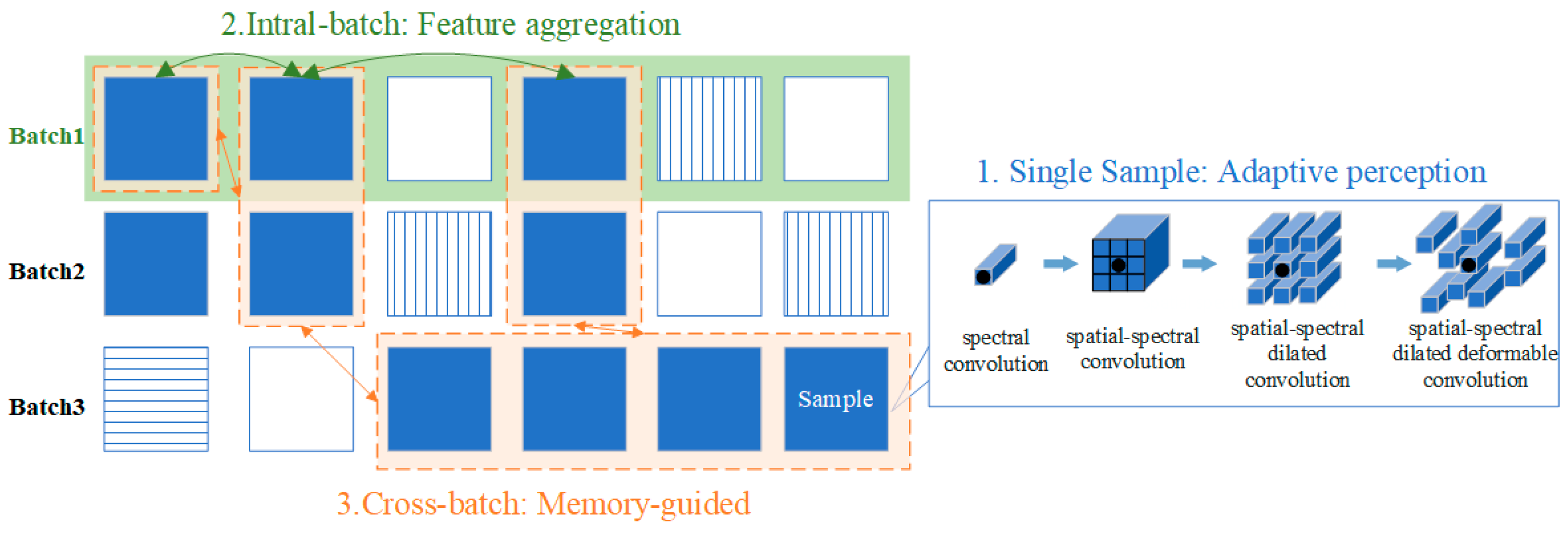
To this end, this paper proposes three complementary global modeling and learning strategies that function at different levels: the single sample level, the intra-batch level, and the cross-batch level, as shown in Figure 1 and

Table 1. Summary of three-level global modeling and learning strategies.

Level	Strategy	Core Components	Objective
Level 1	Single-Sample Globalization	Deformable dilated convolution + Transformer	Enhance global feature understanding within sample
Level 2	Intra-Batch Globalization	Metric learning	Enlarge inter-class distance while reducing intra-class variance
Level 3	Cross-Batch Globalization	Memory-guided strategy	Propagate information across training batches

. As shown in Figure 1, the squares with different filling patterns represent samples from different classes. The green background indicates within-batch samples. The green double arrows aim to pull same-class samples closer via feature augmentation. The orange dashed box highlights same-class samples across different batches. The orange arrows are designed to store features from different batches via the memory mechanism, aiming to facilitate cross-batch feature consistency.

The contributions of this paper are as follows:

• Single-sample globalization: An adaptive perception Transformer is proposed to adapt to the morphological characteristics of land cover features, enlarging the receptive field while mitigating the influence of noise within the HSI patch.
• Intra-batch globalization: A metric-learning-based loss function is designed to enforce a compact and well-separated feature space within each batch.
• Cross-batch globalization: A memory-guided strategy is proposed to store and retrieve same-class features across batches via memory units, enabling the learning of shared patterns in different batches under small-sample.
• Our method achieves superior performance compared to other approaches, obtaining 96.15%, 97.81%, and 99.32% accuracy on three public datasets under severely limited data conditions (less than 1% of the training data).

The remainder of this paper is organized as follows. Section 2 describes the proposed method and the datasets used in the experiments. Section 3 reports the experimental results and provides analysis. Section 4 discusses the influencing factors and the limitations of the proposed method. Finally, Section 5 concludes the paper.

2. Materials and Methods

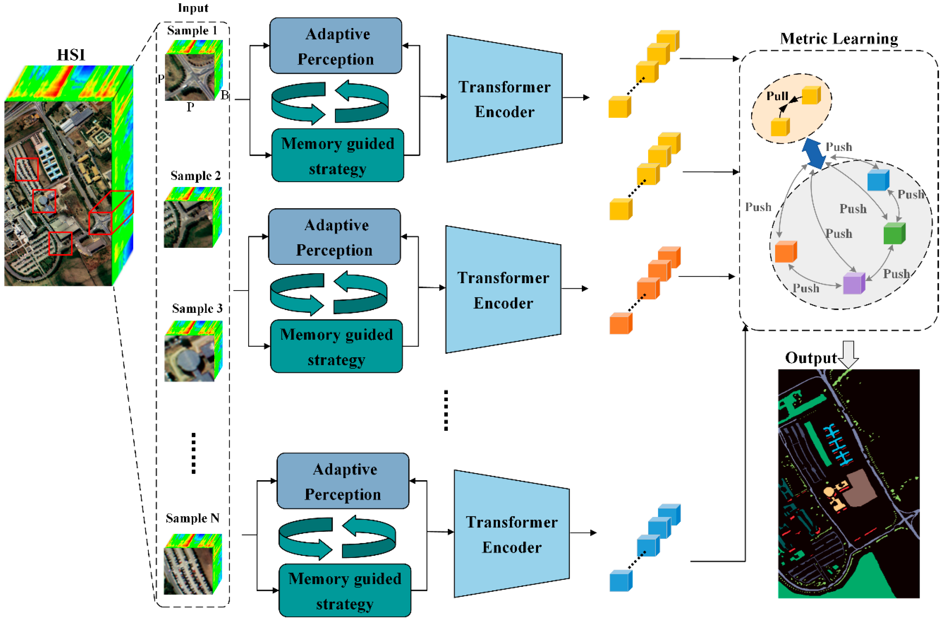
We propose a Memory-Guided Adaptive Perception Transformer (MASSP) model, with its overall architecture illustrated in Figure 2. For each sample point containing B spectral bands, we extract a P × P × B image patch centered at the target pixel as network input, denoted as $X\in R^{P\times P\times B}$. The class of the central pixel of the image patch is used as the sample label, denoted as $Y\in R^{1\times 1\times N}$, where N denotes the total number of classes. The discrepancy between the network’s predictions and the labels is used as the optimization objective. Our method primarily consists of three main components: the adaptive perception Transformer, memory-guided mechanism, and metric learning, which together represent a three-level globalization design, as detailed below.

2.1. Single-Sample Globalization via Adaptive Perception Transformer

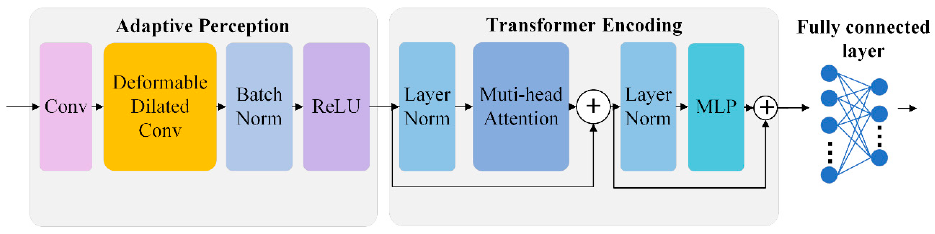
To address CNNs’ limited receptive fields and difficulty in capturing global features, this paper designs the adaptive perception Transformer. As shown in Figure 3, it consists of an adaptive perception module and a transformer encoder. The Adaptive Perception Module integrates deformable convolution with dilated convolution: deformable convolution alters receptive field shape to accommodate geometric deformations, while dilated convolution expands receptive field size to capture long-range context. Their synergy enables simultaneous optimization of both receptive field shape and size, extracting more globalized features. The Transformer encoder leverages multihead self-attention to form fully-connected receptive fields, dynamic attention weights to focus on discriminative regions, and learnable positional encodings to perceive spatial relationships, thereby capturing true global context. Through this “local adaptivity + global modeling” hierarchical feature extraction paradigm, the adaptive perception Transformer achieves superior feature representation capability.

2.1.1. Adaptive Perception Module

We first construct an Adaptive Perception Module that integrates deformable convolution and dilated convolution to enhance feature extraction flexibility and receptive field coverage.

Standard convolution operates on fixed grid locations, limiting its ability to model geometric variations. Deformable convolution addresses this by learning adaptive offsets that allow sampling from non-local positions. To further enlarge the receptive field without increasing parameter count, we incorporate dilated convolution. The standard convolution is defined as follows:

$$F_1={\displaystyle {\sum }_{p_i\in {\mathrm{R}}^{P\times P}}F(p_i)}={\displaystyle {\sum }_{p_i\in {\mathrm{R}}^{P\times P}}{\displaystyle {\sum }_{p_n\in {\mathrm{R}}^{S\times S}}W(p_n)\times X(p_i+p_n)}}$$

(1)

where $p_i$ denotes the position of each pixel in the input image patch, $P\times P$ represents the image patch size, $p_n$ indicates other positions within the convolutional kernel when $p_i$ serves as the kernel’s central pixel, and $S\times S$ is the kernel size.

The deformable dilated convolution implements adaptive perception via dilation rate and offset sampling:

$$F_2={\displaystyle {\sum }_{p_i\in {\mathrm{R}}^{P\times P}}F(p_i)}={\displaystyle {\sum }_{p_i\in {\mathrm{R}}^{P\times P}}{\displaystyle {\sum }_{p_n\in {\mathrm{R}}^{S\times S}}W(p_n)\times F_1(p_i+\gamma \cdot p_n+\Delta p_n))}}$$

(2)

where $\gamma$ denotes the dilation rate, and $\Delta p_n$ denotes the offset value at position $p_n$, learned through convolutional operations.

Finally, batch normalization is applied to obtain normalized feature maps ${F_2}^{\prime }$, followed by ReLU activation via the ReLU function to produce $F_3$.

$${F_2}^{\prime }=BN\left(F_2\right)=\gamma {\displaystyle \frac{F_2-\mu }{\sigma }}+\beta$$

(3)

$$F_3=ReLU\left({F_2}^{\prime }\right)=max\left(0, {F_2}^{\prime }\right)$$

(4)

where $\mu$ and $\sigma$ represent the mean and variance of $F_2$, while $\gamma$ and $\beta$ are learnable parameters. This mechanism enables each sample to dynamically adjust its sampling locations, capturing relevant contextual information from spatially distant but semantically related regions.

2.1.2. Transformer for Global Dependency Modeling

While deformable and dilated convolutions effectively expand receptive fields, they still operate based on local aggregation principles. To capture truly global dependencies across all spatial positions within a patch, we further incorporate a Transformer encoder after the Adaptive Perception module. The Transformer effectively captures correlations between feature sequences using its self-attention mechanism. The input is divided into two parallel branches: one branch first applies LayerNorm for normalization, then computes attention through multihead attention mechanisms before combining the output with the original input through summation. Subsequently, the process splits again into two branches—one branch undergoes LayerNorm normalization before entering an multilayer perceptron, with its output then summed with the other branch.

Firstly, the output from the memory-guided adaptive perception module is flattened and mapped to an embedding vector through a linear layer $I=Linear\left(flatten\left(F_3\right)\right)$, which serves as the input for multihead attention. Three learnable weight parameter matrices $W^Q$, $W^K$, and $W^V$ are defined. The queries Q, keys K, and values V for multihead attention can be expressed as

$$\left\{\begin{array}{l}Q=I{W}^Q\\ K=I{W}^K\\ V=I{W}^V\end{array}\right.$$

(5)

The multihead attention mechanism partitions Q, K, and V into n channels (heads), computing attention for each head separately:

$$\left\{\begin{array}{l}Q=\left\{Q_1,Q_2,\cdots ,Q_n\right\}\\ K=\left\{K_1,K_2,\cdots ,K_n\right\}\\ V=\left\{V_1,V_2,\cdots ,V_n\right\}\end{array}\right.$$

(6)

$$hea{d}_i=\mathrm{softmax}\left({\displaystyle \frac{Q_i{K}_i^T}{\sqrt{d}}}\right)V_i$$

(7)

The scaling factor $\sqrt{d}$ prevents gradient vanishing caused by excessive dot product magnitudes.

The outputs from all n heads are concatenated to form the final multihead attention output:

$$Outpu{t}_{MultiHead}=\mathrm{Concat}\left(hea{d}_1,hea{d}_2,\cdots ,hea{d}_{\mathrm{n}}\right)W^{output}$$

(8)

where $W^{output}$ denotes the output weight matrix.

Following the network architecture, the output of the Transformer encoder can be formulated as

$$H=\mathrm{MLP}\left(\mathrm{LayerNorm}\left(\mathrm{LayerNorm}\left(Outpu{t}_{MultiHead}+I\right) \right)\right)+\left(Outpu{t}_{MultiHead}+I\right)$$

(9)

Finally, the network computes the predicted class for the sample through subsequent processing layers: $Y^{\prime }=\mathrm{Linear}(H)$.

2.2. Intra-Batch Globalization via Metric Learning

While single-sample globalization enables each patch to capture its own global context, it operates independently on each sample and fails to leverage relationships between different samples within the same batch. To address this limitation, we introduce metric learning as our second globalization strategy, which explicitly models inter-sample relationships through feature space organization. Specifically, we propose a multiclass loss that enforces a one-to-one correspondence between anchor-positive sample pairs in the feature space of each batch, thereby achieving intra-batch globalization through discriminative feature learning.

2.2.1. Anchor-Positive Pair Construction

To effectively achieve the above objective, we design a concise and efficient sample pairing strategy. Suppose each training batch contains N samples with feature vectors $H={\left\{h_i\right\}}_{i=1}^N$ and corresponding labels $y={\left\{y_i\right\}}_{i=1}^N\in {\left\{0,1,2,\cdots C-1\right\}}^N$.

First, we construct a positive sample adjacency matrix $M\in {\{0,1\}}^{N\times N}$:

$$M_{ij}=1[y_i=y_j]\cdot 1[i\ne j]$$

(10)

where $1[\cdot ]$ denotes the indicator function. This matrix identifies all sample pairs belonging to the same class.

To establish one-to-one correspondences between anchors and positives, we select one representative pair for each class from these positive pairs. Specifically, we adopt the following strategy: for each class, we select the first occurring sample as the anchor and the second occurring sample as the positive. If a class contains only one sample in the batch, it does not participate in loss computation.

We define the anchor index set $A$ and positive index set $P$ satisfying

$$\left|A\right|=\left|P\right|=K,\forall k\in \left\{0,1,2,\cdots K\right\},y_{Ak}=y_{Pk}$$

(11)

where K denotes the number of classes in the batch that can form valid pairs (i.e., classes containing at least two samples).

2.2.2. Similarity Matrix and Loss Formulation

After completing sample pairing, we apply L₂ normalization to the feature vectors to ensure that similarity computation is unaffected by feature scaling:

$${\widehat{a}}_i={\displaystyle \frac{h_{A_i}}{{‖h_{A_i}‖}_2}},{\widehat{p}}_i={\displaystyle \frac{h_{P_i}}{{‖h_{p_i}‖}_2}}$$

(12)

We then compute the similarity matrix S between anchor features and all positive features:

$$S_{ij}={{\widehat{a}}_i}^{\mathrm{T}}{\widehat{p}}_i$$

(13)

Each row of this matrix corresponds to one anchor’s similarities with all positives.

Based on the similarity matrix described above, we treat it as the logits output of a K-class classification problem. The loss is defined as:

$$L_{MultiClass}=-{\displaystyle \frac{1}{K}}{\displaystyle \sum _{i=1}^{K}log\frac{exp(S_{ii})}{{\displaystyle {\sum }_{\mathrm{j}=1}^{K}exp(S_{ij})}}}$$

(14)

From an optimization perspective, minimizing this loss serves the goal of intra-batch globalization by enforcing that each anchor is pulled toward its corresponding positive from the same class while being pushed away from positives of other classes. This mechanism simultaneously encourages intra-class compactness, where features from the same class cluster closely to maximize anchor-positive similarity, and inter-class separability, where features from different classes are well separated to minimize confusion across classes, thereby achieving global feature structuring within the batch.

2.3. Cross-Batch Globalization via Memory-Guided Strategy

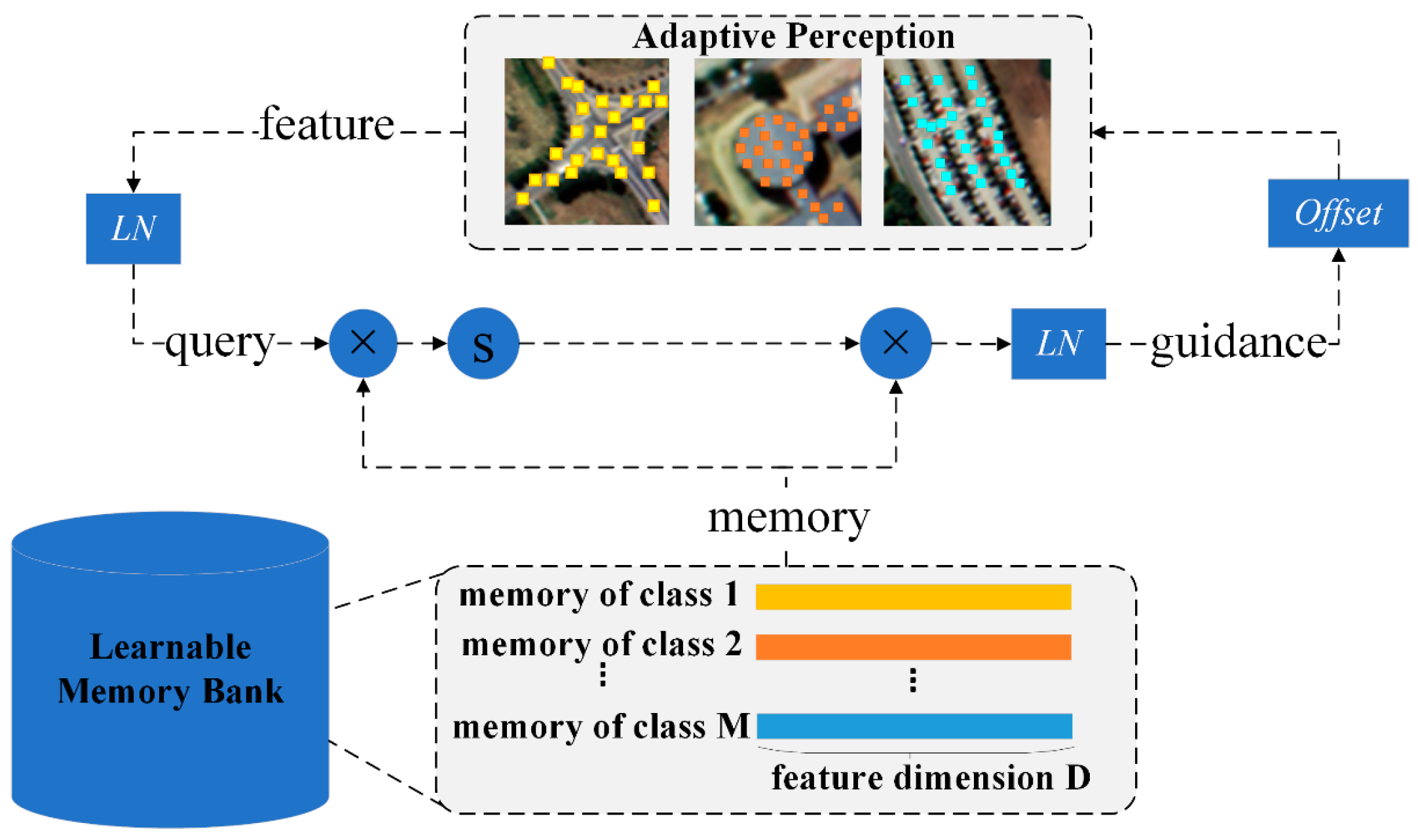
While intra-batch globalization effectively structures feature relationships within each mini-batch, its scope remains limited to the samples present in the current batch. This limitation prevents the model from leveraging historical information in another batch and establishing global feature consistency across the entire dataset. To overcome this, we propose a cross-batch globalization strategy that integrates a memory network to store and retrieve long-range feature dependencies across training iterations. The memory-guided strategy is embedded within the adaptive perception module to integrate cross-batch information. Our method treats the memory bank as a repository of historical feature patterns that guide current feature adaptation. Specifically, as illustrated in Figure 4, a memory unit is constructed to store high-similarity features extracted from previously processed samples belonging to the same class, thereby preserving historical pattern consistency across training iterations. Upon encountering a new patch, it serves as a query to retrieve the most representative feature representations from the memory, effectively bridging past and present feature distributions across batches.

2.3.1. Memory Network

The memory network maintains a learnable memory bank $M\in {ℝ}^{M\times D}$, where M is the capacity of the memory slot and D is the feature dimension. The memory network retrieves and fuses historical information through an attention mechanism.

Given an input feature $f\in {ℝ}^D$, the network first encodes the query through a learnable transformation matrix $W_{q-f}\in {ℝ}^{D\times D}$:

$$q=W_{q-f}•f$$

(15)

The similarity between the query embedding and each memory slot is computed via dot product, followed by softmax normalization to obtain attention weights:

$$a=\mathrm{softmax}\left(q\cdot M^T\right),a\in {ℝ}^M$$

(16)

The retrieved memory guidance is computed as the weighted sum over all memory slots, which is then transformed via an output projection matrix to generate the final memory guidance:

$$guidanc{e}_{memory}={\displaystyle \sum _{k=1}^M{a}_k{M}_k}$$

(17)

This memory network enables the model to dynamically attend to and retrieve relevant historical patterns accumulated across previous training batches, providing cross-batch information for subsequent feature modulation.

2.3.2. Memory-Augmented Adaptive Perception

A memory guidance coefficient $\partial$ (0 < $\partial$ < 1) is introduced to calibrate deformable dilated convolution offsets:

$$offse{t}_{memory}=\Delta p_n+\partial •guidanc{e}_{memory}$$

(18)

where, $\Delta p_n$ denotes the offsets of samples in the current batch, $guidanc{e}_{memory}$ denotes the guidance information retrieved from historical batches via the memory mechanism, and $offse{t}_{memory}$ represents the offsets of the current batch after being corrected and enhanced by the guidance information retrieved from historical batches through the cross-batch memory mechanism.

The output of Adaptive Perception with the memory strategy can be expressed as follows:

$$F_2={\displaystyle {\sum }_{p_i\in {\mathrm{R}}^{P\times P}}F(p_i)}={\displaystyle {\sum }_{p_i\in {\mathrm{R}}^{P\times P}}{\displaystyle {\sum }_{p_n\in {\mathrm{R}}^{S\times S}}W(p_n)\times F_1(p_i+\gamma \cdot p_n+offse{t}_{memory}(p_n))}}$$

(19)

The Adaptive Perception with the memory strategy in Equation (19) replaces the original F₂ computation in Equation (2) before proceeding with subsequent steps.

2.4. Data Description

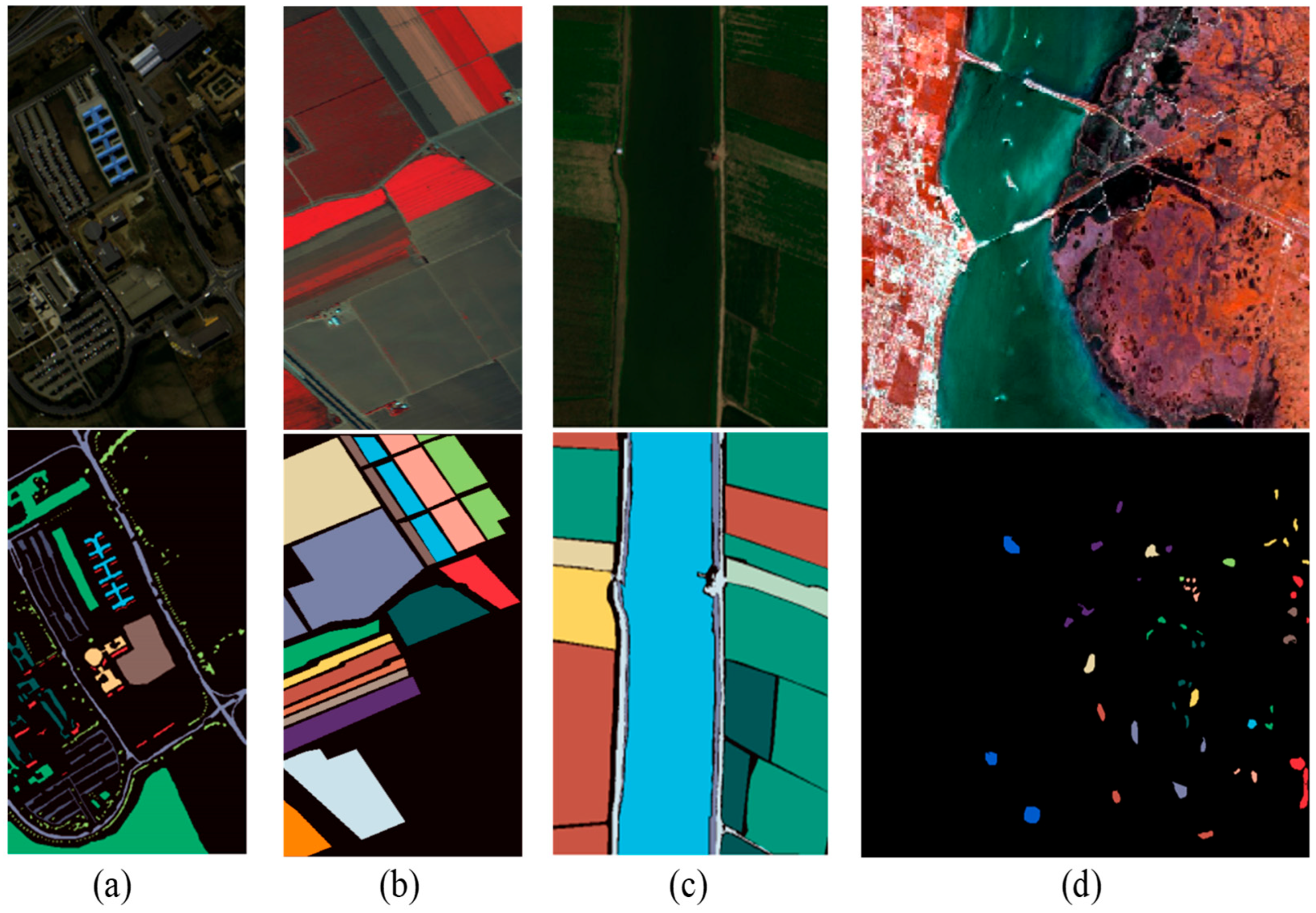
To validate the performance of the proposed model, this paper selects three widely used and diverse HSI datasets from different countries and regions: Pavia University (PU), SaliLMSS (SA), WHU-LongKou (WHU-LK) and Kennedy Space Center (KSC). As shown in Figure 5, the first three datasets possess relatively high spatial resolution (0.463 m/pixel~3.7 m/pixel), which naturally gives rise to spatially compact and contiguous class distributions. In contrast, the lower spatial resolution of KSC (18 m/pixel) leads to a more fragmented and spatially dispersed arrangement of land cover classes.

(1)

PU: The dataset was acquired in 2001 over Pavia University Northern Italy, using the Reflective Optics System Imaging Spectrometer (ROSIS). The ROSIS was developed jointly by Dornier Satellite Systems (in Ottobrunn, German), GKSS Research Centre (in Geesthacht, German) and German Aerospace Center (in Oberpfaffenhofen, German). As shown in Figure 5a, the image has dimensions of 610 × 340 pixels with a spatial resolution of 1.3 m/pixel. It contains 115 spectral bands ranging from 380 to 860 nm. The dataset comprises 42,776 annotated samples spanning 9 land cover classes, including asphalt, meadows, gravel, and shadows.

(2)

SA: The dataset was collected in 1998 over the SaliLMSS Valley, California, USA, using the Airborne Visible/Infrared Imaging Spectrometer (AVIRIS). The AVIRIS was developed by NASA’s Jet Propulsion Laboratory in Pasadena, CA, USA. As shown in Figure 5b, it has dimensions of 512 × 217 pixels and a spatial resolution of 3.7 m/pixel. The original 224 spectral bands (400–2500 nm) were reduced to 204 after removing water-vapor-affected bands. It comprises 54,129 labeled samples spanning 16 land cover classes dominated by fallow fields, stubble, celery, and lettuce.

(3)

WHU-LK: The dataset was acquired in 2018 over Longkou Town, Hubei Province, China, using a DJI Matrice 600 Pro drone equipped with a Headwall Nano hyperspectral imager, and the system is manufactured by DJI in Shenzhen, China. As shown in Figure 5c, it has dimensions of 550 × 400 pixels and a spatial resolution of 0.463 m/pixel. It includes 270 spectral bands (400–1000 nm). The dataset comprises 204,542 annotated samples spanning 9 land cover classes, including water, weeds, corn, and rice.

(4)

KSC: The dataset was acquired by the AVIRIS sensor on 23 March 1996. The acquisition site was the Kennedy Space Center in Florida. The flight altitude was approximately 20 km. We adopt the corrected KSC dataset. It has dimensions of 512 × 614 pixels and a spatial resolution of 18 m/pixel. The sensor covers 224 spectral bands. Each band has a width of 10 nm. The wavelength range extends from 400 to 2500 nm. It comprises 5211 labeled samples spanning 13 land cover classes dominated by salt marsh, mud flats, hardwood and water.

For the PU and SA datasets, 1% of the labeled samples per class were randomly selected as the training set, with the remaining samples divided into validation and test sets. For the WHU-LK dataset, 0.5% of the samples were used for training.

Table 2. The number of training, validation, and test samples in the PU dataset (1%).

No.	Name	Total	Training	Validation	Test	Color
1	Asphalt	6631	66	67	6498
2	Meadows	18,649	186	187	18,276
3	Gravel	2099	20	22	2057
4	Trees	3064	30	32	3002
5	Painted metal sheets	1345	13	14	1318
6	Bare Soil	5029	50	51	4928
7	Bitumen	1330	13	14	1303
8	Self-Blocking Bricks	3682	36	38	3608
9	Shadows	947	9	10	928
All Classes		42,776	423	435	41,918

,

Table 3. The number of training, validation, and test samples in the SA dataset (1%).

No.	Name	Total	Training	Validation	Test	Color
1	Brocoli_green_weeds_1	2009	20	21	1968
2	Brocoli_green_weeds_2	3726	37	38	3651
3	Fallow	1977	19	21	1937
4	Fallow_rough_plow	1394	13	15	1366
5	Fallow_smooth	2678	26	28	2624
6	Stubble	3959	39	41	3879
7	Celery	3579	35	37	3507
8	Grapes_untrained	11,271	112	114	11,045
9	Soil_vinyard_develop	6203	62	63	6078
10	Corn_senesced_green_weeds	3278	32	34	3212
11	Lettuce_romaine_4wk	1068	10	12	1046
12	Lettuce_romaine_5wk	1927	19	20	1888
13	Lettuce_romaine_6wk	916	9	10	897
14	Lettuce_romaine_7wk	1070	10	12	1048
15	Vinyard_untrained	7268	72	74	7122
16	Vinyard_vertical trellis	1807	18	19	1770
All Classes		54,130	533	559	53,038

,

Table 4. The number of training, validation, and test samples in the WHU-LK dataset (0.5%).

No.	Name	Total	Training	Validation	Test	Color
1	Corn	34,511	172	174	34,165
2	Cotton	8374	41	43	8290
3	Sesame	3031	15	16	3000
4	Broad-leaf soybean	63,212	316	317	62,579
5	Narrow-leaf soybean	4151	20	22	4109
6	Rice	11,854	59	60	11,735
7	Water	67,056	335	336	66,385
8	Roads and houses	7124	35	37	7052
9	Mixed weed	5229	26	27	5176
All Classes		204,542	1022	1032	202,496

and

Table 5. The number of training, validation, and test samples in the KSC dataset (1%).

No.	Name	Total	Training	Validation	Test	Color
1	Scrub	761	7	8	746
2	Willow swamp	243	2	3	238
3	CP hammock	256	3	2	251
4	Slash pine	252	3	2	247
5	Oak/Broadleaf	161	1	2	158
6	Hardwood	229	3	2	224
7	Swamp	105	1	1	103
8	Graminoid marsh	431	4	5	422
9	Spartina marsh	520	5	5	510
10	Cattail marsh	404	4	4	396
11	Salt marsh	419	4	4	411
12	Mud flats	503	5	5	493
13	Water	927	10	9	908
All Classes		5211	52	52	5107

detail the distribution of training, validation, and test samples across classes.

2.5. Experimental Setup and Evaluation Metrics

All experiments were conducted on a platform with an Ubuntu operating system, PyTorch 2.4.1 framework, and RTX 4090 GPU. The detailed model training parameters are as follows: total epochs were set to 300, patch size to 7 ×  7, batch size to 64, optimizer to stochastic gradient descent (SGD) with an initial learning rate of 0.001, momentum of 0.9, and weight decay of 0.0001. Empirically, the memory guidance coefficient is a value no greater than 0.1. In our experiments, we set it to 0.1 on SA, 0.05 on PU and WHU-LK, and 0.025 on KSC.

The labeled samples are randomly partitioned into training, validation, and test sets. For the PU, SA, and KSC datasets, the proportions are 1%, 1%, and 98%, respectively. For the WHU-HK dataset, the proportions are 5%, 1%, and 94%, respectively.

During training, the surrounding 7 × 7 patches of the selected training samples are cropped as network inputs. These patches are fed into the Adaptive Perception Transformer in mini-batches of 64. A memory guidance mechanism is employed to store and aggregate features of samples from the same class across different batches, enabling global feature representation. The network is optimized by minimizing a metric-learning-based loss function, with parameters updated via the SGD optimizer. The validation set guides hyperparameter selection and dynamically saves the checkpoint with the lowest validation loss. Training is terminated upon convergence, which is achieved at approximately 300 epochs in our experiments. The pseudocode for training the three-level globalization strategy is presented in

Table 6. Pseudocode for training the three-level globalization strategy.

Level/Step	Operation
Input	Training set X, batch size B, epochs T, memory capacity M, coefficient η
Initialization	Model parameters θ
Training	for epoch = 1 to T do:
	for each batch do:
Level 1: Single-Sample	Extract adaptive features via deformable dilated conv
	Encode global dependencies via Transformer multihead self-attention
	Obtain final feature
Level 2: Intra-Batch	Build positive pairs, select anchor and positive per class
	L2-normalize features
	Compute similarity matrix
	Compute intra-batch loss: pull same-class closer, push different-class apart
Level 3: Cross-Batch	Query memory bank, compute attention weights
	Retrieve historical memory guidance
	Calibrate offsets with memory information
	Obtain memory-augmented features
	Compute cross-batch consistency loss: pull current features close to historical same-class features
Joint Optimization	Total loss = classification loss + intra-batch loss + cross-batch loss; Update model parameters
Memory Update	Update memory bank with momentum features
	end for
	end for
Output	Return optimal model θ* (θ* denotes the optimal model parameters)

. During testing, the model parameters that attained the lowest validation loss are loaded, and the remaining 98% of the samples are fed into this best-performing network to obtain predicted labels for quantitative evaluation.

The performance evaluation of the proposed method relies on three widely accepted metrics: overall accuracy (OA), average accuracy (AA), and the kappa coefficient (kappa), as shown in the following mathematical expressions. To ensure validity and reliability, each experiment was repeated five times with independently randomized training sets. Mean values and standard deviations of these metrics were calculated from five independent trials.

$$OA={\displaystyle \frac{{\displaystyle \sum _{i=1}^{\mathrm{N}}{\widehat{y}}_i}}{{\displaystyle \sum _{i=1}^{\mathrm{N}}{y}_i}}}$$

(20)

$$AA={\displaystyle \frac{1}{N}}{\displaystyle \sum _{i=1}^{\mathrm{N}}\left(\frac{{\widehat{y}}_i}{y_i}\right)}$$

(21)

$$P_o=OA, P_{\mathrm{e}}={\displaystyle \frac{{\displaystyle \sum _{i=1}^{\mathrm{N}}\left({\displaystyle \sum _{j=1}^{\mathrm{N}}{M}_{i,j}{\displaystyle \sum _{j=1}^{\mathrm{N}}{M}_{j,i}}}\right)}}{{\displaystyle \sum _{i=1}^{\mathrm{N}}{\displaystyle \sum _{j=1}^{\mathrm{N}}{M}_{i,j}}}}}$$

(22)

$$\mathrm{Kappa}={\displaystyle \frac{P_o-P_{\mathrm{e}}}{1-P_{\mathrm{e}}}}$$

(23)

where N represents the number of classes. For the i-th class, ${\widehat{y}}_i$ represents the number of correctly predicted labels, $y_i$ represents the total number of labels. The elements $M_{i,j}$ and $M_{j,i}$ in the confusion matrix represent the number of samples where the actual class i is predicted as class j and the actual class j is predicted as class i, respectively. P_o and e denote the observed agreement and expected agreement, respectively.

3. Results

3.1. Comparative Methods and Setup

In order to evaluate the performance of the proposed method, five representative and competitive deep-learning-based HSI classification algorithms are used for comparison, including Attention Network with Bidirectional Long Short-Term Memory (ABLSTM) [49], Spectral Former (SF) [24], Adaptive Morphology Filter (AMF) [50], Lightweight Multiscale Neural Architecture Search (LMSS) [51], Lightweight Domain Generalization Network (L-DGNet) [52], Dual-branch Subpixel-guided Network (DSNet) [53], Subpixel Spectral Variability Network (S²VNet) [54], Cascaded Spatial Cross-Attention Network (CSCANet) [41], and Joint Domain Adaptation With Weight Self-Learning (JDAWSL) [55], respectively.

(1)

ABLSTM employs forward and backward LSTM layers to establish bidirectional memory pathways, endowing it with the ability to selectively retain or forget long-sequence information. In addition, a spatial–spectral attention mechanism is integrated into the network to adaptively weigh information across different positions and bands, thereby achieving adaptive perception [49].

(2)

SF is the first architecture to apply a Transformer to hyperspectral classification. The multihead self-attention mechanism inherently provides global perception, enabling every position to directly attend to all others to capture global spectral–spatial dependencies. The grouped spectral embedding module embeds adjacent bands in groups to fully exploit spectral local continuity. The cross-layer adaptive fusion module delivers shallow information to deeper layers via “soft residual” skip connections [24].

(3)

AMF is reparameterizable into an equivalent binary morphological filter, enabling depthwise adaptive spatial feature extraction from hyperspectral images. Stacking multiple instances further broadens the receptive field toward global contextual perception [50].

(4)

The core of LMSS is not a manually fixed network, but an optimal architecture automatically discovered via neural architecture search within a predefined multiscale search space, thus removing the subjectivity of hand-crafted design [51].

(5)

L-DGNet is a method for few-shot hyperspectral image classification. Its core lies in introducing the semantic information of text labels as an auxiliary supervisory signal, and guiding the model to learn more robust category semantic features through language–visual cross-modal representation alignment, thereby enhancing the model’s generalization capability with only a small number of labeled samples [52].

(6)

DSNet adopts a dual-branch architecture that bridges physical models and deep learning. One branch employs a deep autoencoder to automatically extract sub-pixel physical information, such as endmembers and abundances. The other branch is responsible for extracting convolutional deep-learning features. These two branches are then fused through a sub-pixel fusion module, which ensures high-quality integration of the complementary information [53].

(7)

S²VNet models subpixel-scale spectral mixing and variability, and fuses physically derived abundances and spectral similarity with data-driven semantic features to yield robust classification under mixed pixel conditions [54].

(8)

The core of CSCANet is a cascaded spatial cross-attention module, which is designed to directly bridge local features and the global context. This mechanism enables each spatial position to be aware of the holistic scene information [41].

(9)

JDAWSL is a cross-domain few-shot hyperspectral image classification method. It combines a domain discriminator with a domain projector to suppress domain-specific features while aligning domain-shared features. An adaptive learner is also introduced to dynamically adjust loss weights [55].

For a fair comparison, all competing methods were trained with the same number of training samples as our proposed method, i.e., 1% of the total samples for the PU, SA, and KSC datasets, and 0.5% for the WHU-HK dataset. In addition, all methods shared the same total epochs (300), patch size (7 × 7), and batch size (64). Other method-specific hyperparameters were set according to their publications.

3.2. Classification Results and Analysis

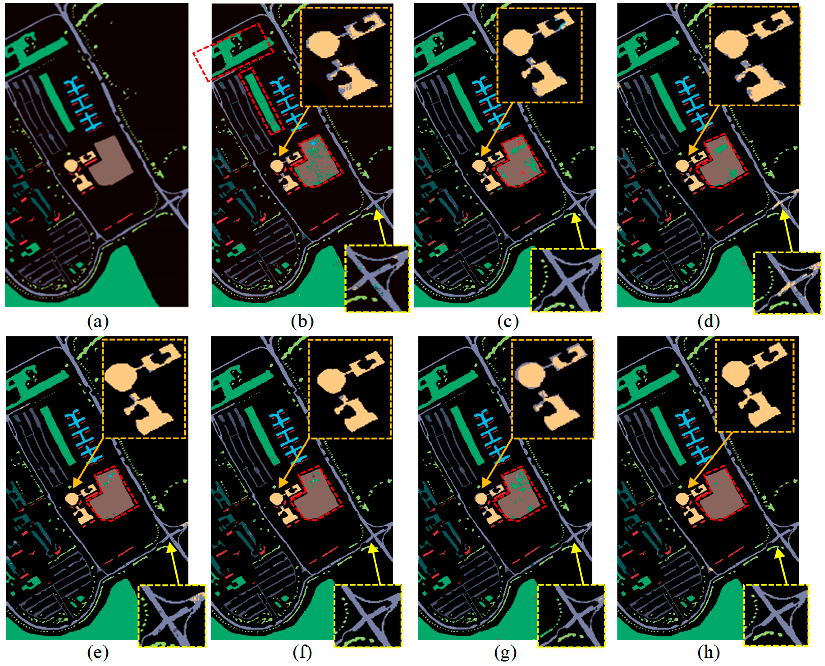
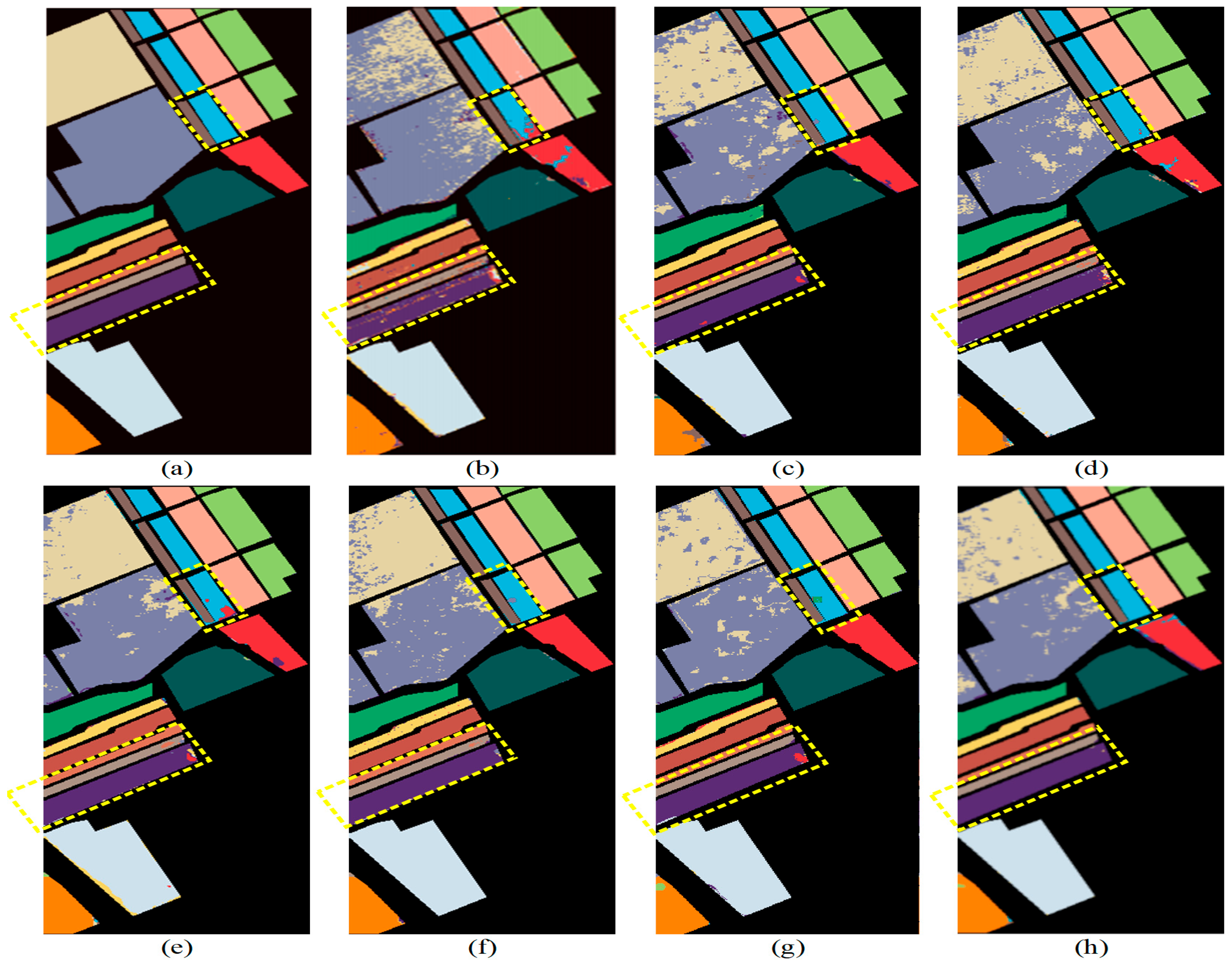
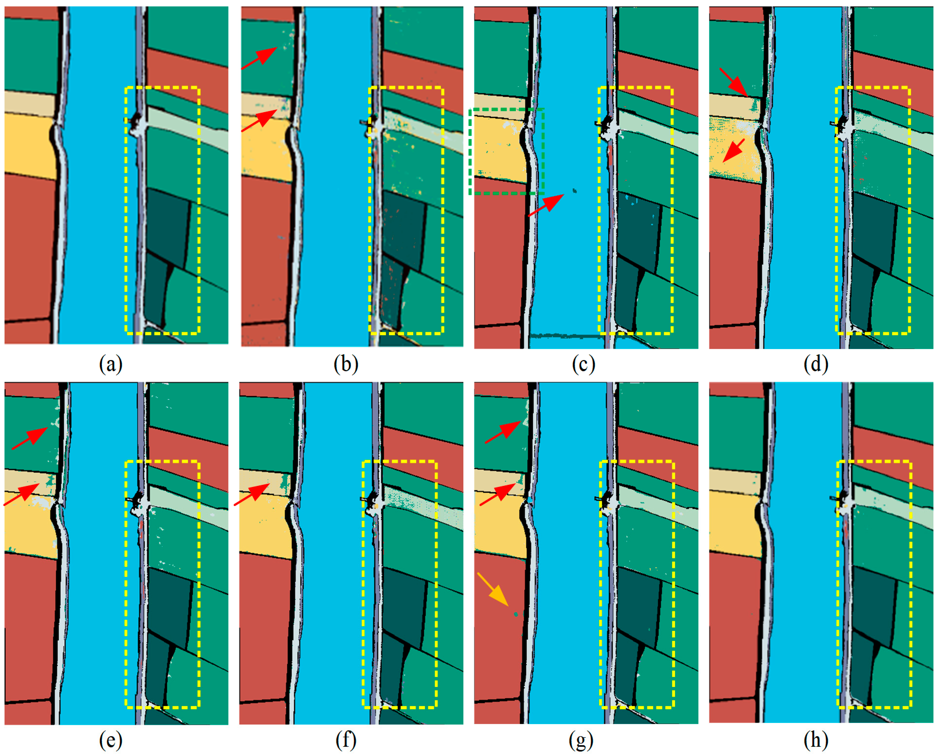
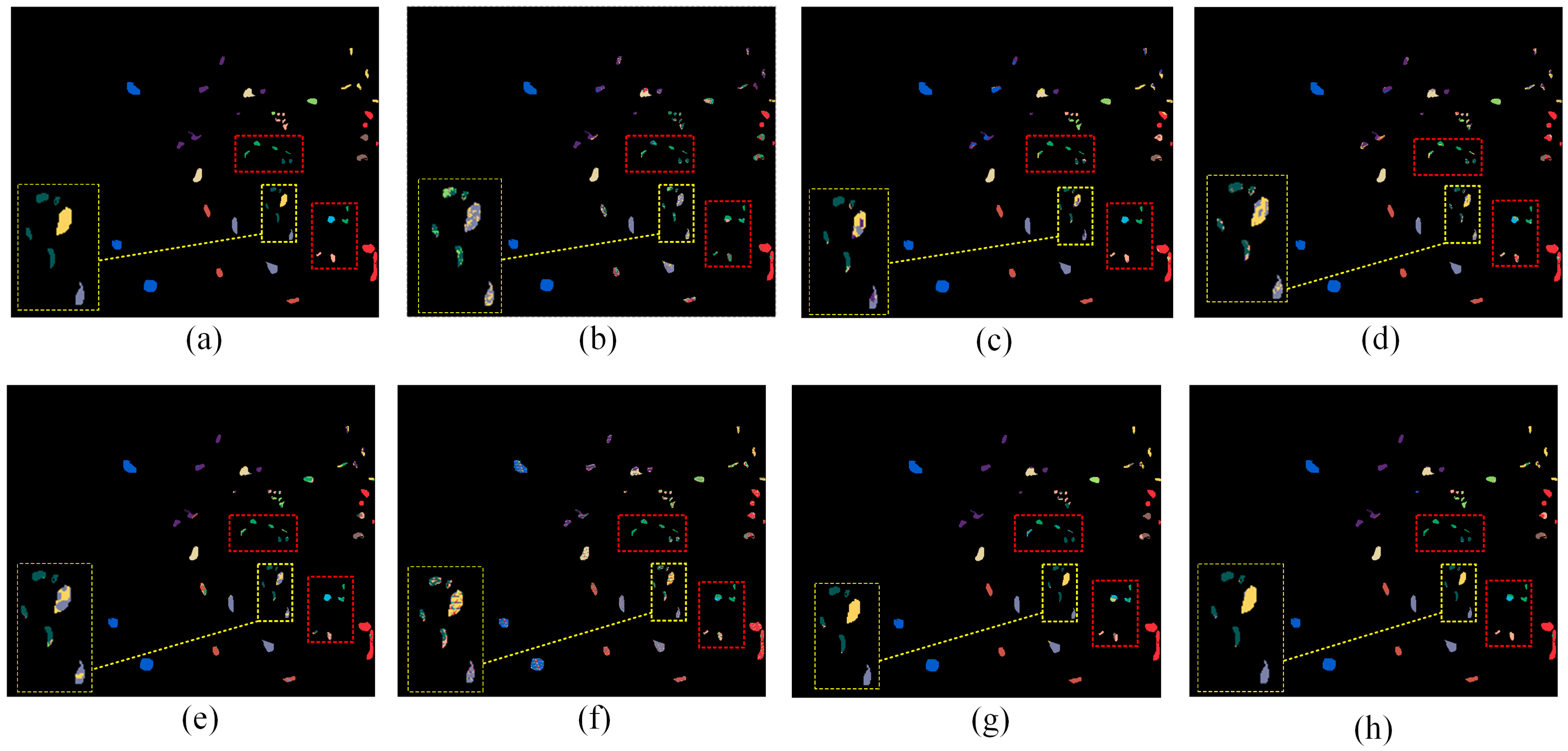
Figure 6, Figure 7, Figure 8 and Figure 9 present qualitative comparative experimental results on four public datasets, where (a) shows displays ground truth maps, (b–g) illustrate classification results from comparison methods, and (h) presents our method’s result. Quantitative performance metrics are detailed in

Table 7. Classification results of different methods on the PU dataset with 1% training sample.

Class	ABLSTM	SF	AMF	LMSS	L-DGNet	DSNet	CSCANet	S2VNet	JDAWSL	Ours
1	90.75 ± 2.14	86.31 ± 2.55	97.47 ± 1.58	93.17 ± 1.42	93.74 ± 2.10	95.63 ± 0.68	97.89 ± 0.56	95.69 ± 2.42	96.67 ± 0.89	97.82 ± 0.80
2	97.86 ± 0.80	97.05 ± 1.12	99.61 ± 0.21	97.62 ± 1.48	98.13 ± 1.16	99.56 ± 0.15	99.82 ± 0.13	99.43 ± 0.49	97.24 ± 0.99	99.42 ± 0.31
3	66.95 ± 6.54	70.06 ± 7.53	89.31 ± 9.52	83.20 ± 5.48	67.03 ± 12.1	84.43 ± 6.17	88.04 ± 4.52	74.21 ± 10.06	83.27 ± 3.91	89.56 ± 2.63
4	91.91 ± 2.66	91.94 ± 1.58	96.90 ± 1.83	94.65 ± 0.96	95.68 ± 2.79	96.06 ± 0.90	97.48 ± 0.68	94.81 ± 2.82	91.09 ± 0.64	97.92 ± 0.27
5	98.21 ± 1.17	100.00 ± 0	99.98 ± 0.03	99.71 ± 0.43	99.79 ± 0.19	99.74 ± 0.48	99.97 ± 0.04	99.74 ± 0.34	99.17 ± 1.30	100.00 ± 0
6	80.15 ± 2.60	78.41 ± 4.06	98.20 ± 1.34	90.42 ± 5.36	87.15 ± 6.41	97.91 ± 0.84	96.63 ± 1.53	97.57 ± 2.38	86.56 ± 2.50	97.87 ± 0.98
7	80.84 ± 3.83	62.47 ± 2.92	90.51 ± 5.71	90.70 ± 2.10	86.82 ± 7.46	88.60 ± 9.24	95.53 ± 1.92	91.01 ± 8.36	86.48 ± 3.60	95.81 ± 5.24
8	86.85 ± 2.95	78.73 ± 8.10	90.74 ± 4.06	94.47 ± 3.02	87.74 ± 4.41	93.77 ± 1.69	91.61 ± 4.03	95.93 ± 2.35	93.93 ± 0.77	95.86 ± 0.45
9	98.99 ± 0.48	95.93 ± 0.96	99.40 ± 0.46	61.85 ± 5.88	98.92 ± 0.90	99.18 ± 1.28	98.30 ± 2.77	97.03 ± 3.61	98.17 ± 2.05	99.76 ± 0.13
OA (%)	91.29 ± 1.07	88.92 ± 1.07	97.37 ± 0.36	93.95 ± 0.26	93.28 ± 1.15	96.92 ± 0.56	97.53 ± 0.18	96.45 ± 0.84	94.23 ± 0.46	98.00 ± 0.33
AA (%)	88.06 ± 0.78	84.54 ± 1.37	95.79 ± 1.15	89.53 ± 0.91	90.56 ± 1.82	94.99 ± 1.19	96.14 ± 0.42	93.93 ± 1.32	92.51 ± 0.56	97.11 ± 0.13
Kappa	88.37 ± 1.43	85.21 ± 1.46	96.52 ± 0.48	91.96 ± 0.33	91.06 ± 1.54	95.92 ± 0.74	96.72 ± 0.24	95.30 ± 1.11	92.32 ± 0.60	97.35 ± 0.44

,

Table 8. Classification performance of different methods on the SA dataset (using 1% of the total data as the training set).

Class	ABLSTM	SF	AMF	LMSS	L-DGNet	DSNet	CSCANet	S2VNet	JDAWSL	Ours
1	94.36 ± 7.76	95.71 ± 1.24	97.43 ± 3.39	96.84 ± 5.49	99.37 ± 0.55	100.00 ± 0	99.91 ± 0.11	99.56 ± 0.52	99.23 ± 0.76	100.00 ± 0
2	98.39 ± 0.92	99.48 ± 0.26	99.87 ± 0.14	98.87 ± 0.80	96.01 ± 5.33	99.46 ± 0.38	99.68 ± 0.16	99.89 ± 0.15	99.89 ± 0.14	99.92 ± 0.15
3	88.49 ± 4.19	95.19 ± 1.28	97.61 ± 0.39	96.74 ± 2.06	94.32 ± 2.60	97.31 ± 1.14	99.66 ± 0.61	98.32 ± 1.46	99.28 ± 1.03	94.74 ± 6.27
4	92.96 ± 11.13	94.55 ± 2.30	97.77 ± 2.38	97.77 ± 1.34	98.39 ± 1.43	98.11 ± 1.62	98.52 ± 0.60	99.24 ± 0.25	96.66 ± 3.28	98.74 ± 0.73
5	96.14 ± 3.08	92.20 ± 4.00	96.30 ± 2.96	95.37 ± 3.31	98.23 ± 1.23	96.55 ± 2.30	98.55 ± 1.09	97.31 ± 1.39	98.34 ± 1.84	99.06 ± 1.26
6	98.03 ± 1.73	99.42 ± 0.58	99.99 ± 0.01	99.67 ± 0.37	99.90 ± 0.15	99.96 ± 0.03	99.79 ± 0.41	99.97 ± 0.04	99.89 ± 0.20	100.00 ± 0
7	99.03 ± 0.42	98.25 ± 0.70	99.82 ± 0.20	99.53 ± 0.41	99.42 ± 0.29	99.83 ± 0.10	99.85 ± 0.09	99.95 ± 0.05	99.48 ± 0.48	99.93 ± 0.08
8	80.59 ± 10.63	84.97 ± 2.03	90.15 ± 3.33	86.28 ± 3.47	89.22 ± 2.01	92.54 ± 1.38	92.73 ± 2.65	91.73 ± 2.13	89.24 ± 2.17	92.46 ± 0.79
9	97.98 ± 1.53	96.76 ± 1.44	99.27 ± 1.15	99.75 ± 0.39	99.56 ± 0.11	98.57 ± 2.09	99.90 ± 0.02	99.67 ± 0.40	99.62 ± 0.32	99.92 ± 0.14
10	83.41 + 1.25	89.64 ± 2.80	94.84 ± 1.53	95.90 ± 1.63	95.83 ± 1.66	95.60 ± 1.48	97.31 ± 1.35	95.33 ± 2.02	95.70 ± 0.95	97.73 ± 1.49
11	62.71 ± 32.59	90.05 ± 1.77	98.17 ± 0.82	98.68 ± 0.85	95.34 ± 4.66	97.88 ± 1.26	98.19 ± 1.14	98.28 ± 0.43	95.43 ± 3.80	99.20 ± 0.34
12	97.70 ± 1.86	98.47 ± 1.38	99.57 ± 0.62	99.25 ± 0.77	99.43 ± 1.09	100.00 ± 0	99.69 ± 0.51	99.99 ± 0.02	99.70 ± 0.39	99.92 ± 0.12
13	97.39 ± 1.42	92.61 ± 7.78	98.26 ± 1.95	98.86 ± 1.30	99.44 ± 0.29	98.13 ± 2.85	97.06 ± 1.99	98.31 ± 2.08	99.46 ± 0.28	99.29 ± 0.81
14	70.49 ± 33.40	96.57 ± 2.67	95.98 ± 2.62	97.73 ± 2.26	96.17 ± 0.98	96.11 ± 2.02	94.68 ± 4.00	97.01 ± 2.16	98.63 ± 0.96	99.03 ± 0.34
15	42.38 ± 23.59	79.07 ± 4.88	87.07 ± 5.93	80.49 ± 4.81	89.37 ± 3.60	87.60 ± 4.14	90.36 ± 4.73	87.84 ± 3.06	84.58 ± 2.73	87.86 ± 1.66
16	89.03 ± 7.16	92.72 ± 4.21	95.92 ± 3.83	90.95 ± 4.36	95.09 ± 2.62	94.65 ± 3.99	98.15 ± 0.48	95.16 ± 3.61	97.75 ± 1.25	96.71 ± 2.18
OA (%)	83.85 ± 1.66	91.32 ± 0.78	95.08 ± 0.58	93.17 ± 0.50	94.98 ± 0.42	95.65 ± 0.18	96.19 ± 0.45	95.80 ± 0.49	94.90 ± 0.49	96.21 ± 0.34
AA (%)	86.82 ± 3.08	93.48 ± 0.78	96.75 ± 0.56	95.79 ± 0.48	96.57 ± 0.68	97.02 ± 0.24	97.77 ± 0.33	97.35 ± 0.28	97.06 ± 0.37	97.78 ± 0.45
Kappa	81.96 ± 1.90	90.34 ± 0.88	94.52 ± 0.65	92.40 ± 0.56	94.41 ± 0.46	95.16 ± 0.20	95.31 ± 0.50	95.32 ± 0.54	94.32 ± 0.55	95.78 ± 0.38

,

Table 9. Classification performance of different methods on the WHU-LK dataset (using 0.5% of the total data as the training set).

Class	ABLSTM	SF	AMF	LMSS	L-DGNet	DSNet	CSCANet	S2VNet	JDAWSL	Ours
1	98.28 ± 2.01	99.58 ± 0.16	99.79 ± 0.10	99.79 ± 0.10	99.65 ± 0.21	99.81 ± 0.08	99.95 ± 0.03	99.91 ± 0.06	99.73 ± 0.15	99.86 ± 0.07
2	91.25 ± 3.13	91.85 ± 3.05	97.64 ± 1.58	97.85 ± 1.82	90.43 ± 6.30	94.44 ± 2.66	98.54 ± 0.95	96.81 ± 0.95	96.08 ± 1.08	98.51 ± 0.92
3	80.49 ± 7.02	94.31 ± 1.06	95.70 ± 1.14	97.34 ± 1.69	90.03 ± 8.36	93.81 ± 2.12	93.76 ± 2.96	92.95 ± 3.28	95.60 ± 1.61	96.32 ± 1.69
4	98.20 ± 0.76	98.12 ± 0.56	99.45 ± 0.15	99.54 ± 0.18	98.55 ± 0.65	99.20 ± 0.32	99.55 ± 0.14	99.25 ± 0.08	99.29 ± 0.22	99.59 ± 0.17
5	81.61 ± 2.96	83.88 ± 3.61	91.99 ± 1.48	92.46 ± 3.14	82.85 ± 10.82	88.49 ± 3.94	93.68 ± 4.72	90.71 ± 5.26	91.32 ± 3.14	93.78 ± 2.04
6	95.82 ± 1.33	97.08 ± 1.58	99.14 ± 0.59	90.04 ± 1.62	99.08 ± 0.94	99.48 ± 0.41	99.76 ± 0.15	99.53 ± 0.38	99.73 ± 0.18	99.59 ± 0.23
7	99.96 ± 0.03	99.96 ± 0.03	99.96 ± 0.02	99.28 ± 0.69	99.98 ± 0.01	99.99 ± 0.00	99.99 ± 0.01	99.95 ± 0.04	99.96 ± 0.04	99.98 ± 0.02
8	92.83 ± 1.84	89.52 ± 3.92	94.83 ± 2.47	96.95 ± 1.43	92.81 ± 3.47	96.40 ± 1.18	95.42 ± 1.60	96.13 ± 2.02	91.87 ± 1.75	97.40 ± 0.93
9	68.59 + 8.66	75.43 ± 4.53	89.32 ± 4.33	90.37 ± 2.79	90.25 ± 2.55	90.59 ± 3.64	94.68 ± 2.22	91.06 ± 2.37	91.15 ± 2.43	93.54 ± 2.92
OA (%)	96.83 ± 0.39	97.43 ± 0.34	98.96 ± 0.19	98.38 ± 0.25	98.05 ± 0.37	98.77 ± 0.19	99.26 ± 0.17	98.92 ± 0.24	98.79 ± 0.16	99.32 ± 0.20
AA (%)	89.67 ± 1.14	92.19 ± 0.80	96.43 ± 0.74	95.96 ± 0.55	93.74 ± 2.23	95.80 ± 0.52	97.26 ± 0.96	96.26 ± 1.06	96.08 ± 0.61	97.62 ± 0.71
Kappa	95.82 ± 0.51	96.61 ± 0.45	98.63 ± 0.25	97.86 ± 0.33	97.43 ± 0.49	98.38 ± 0.25	99.02 ± 0.23	98.58 ± 0.32	98.41 ± 0.21	99.11 ± 0.26

and

Table 10. Classification performance of different methods on the KSC dataset (using 1% of the total data as the training set).

Class	ABLSTM	SF	AMF	LMSS	L-DGNet	DSNet	CSCANet	S2VNet	JDAWSL	Ours
1	90.08 ± 3.13	91.24 ± 9.07	95.67 ± 2.36	92.05 ± 4.82	94.64 ± 4.37	90.97 ± 7.27	77.21 ± 5.02	94.46 ± 2.60	98.74 ± 0.54	98.30 ± 0.91
2	47.34 ± 25.83	39.08 ± 18.54	51.40 ± 29.12	76.05 ± 9.29	51.26 ± 21.06	66.81 ± 3.09	61.34 ± 17.05	82.21 ± 12.69	70.59 ± 10.21	78.43 ± 26.71
3	60.29 ± 8.27	53.92 ± 8.00	78.75 ± 13.70	74.90 ± 16.92	51.53 ± 18.36	70.92 ± 16.49	52.86 ± 0.68	90.84 ± 8.99	91.60 ± 5.05	95.62 ± 1.42
4	31.04 ± 20.70	39.54 ± 6.26	39.27 ± 12.19	64.10 ± 15.04	37.11 ± 0.69	44.13 ± 9.82	49.80 ± 16.62	59.65 ± 8.11	56.99 ± 21.56	54.96 ± 2.98
5	29.54 ± 19.07	32.91 ± 22.72	41.14 ± 24.30	52.32 ± 17.39	39.45 ± 29.49	27.64 ± 17.63	35.44 ± 23.02	68.99 ± 3.10	51.46 ± 20.14	55.91 ± 23.26
6	19.05 ± 5.31	54.91 ± 6.32	52.38 ± 18.46	52.98 ± 33.78	51.79 ± 11.69	60.27 ± 0.36	40.77 ± 9.76	78.12 ± 8.85	75.09 ± 18.60	64.14 ± 12.73
7	15.53 ± 14.47	78.64 ± 15.06	80.58 ± 13.24	73.79 ± 17.92	61.49 ± 29.93	83.50 ± 23.34	42.72 ± 12.46	50.16 ± 37.29	77.84 ± 20.65	84.47 ± 4.82
8	24.72 ± 6.70	41.94 ± 13.64	53.71 ± 21.21	54.03 ± 7.35	40.68 ± 9.96	44.15 ± 6.74	46.37 ± 12.96	55.69 ± 6.04	87.25 ± 11.50	66.43 ± 15.92
9	82.68 ± 10.90	81.50 ± 8.52	91.31 ± 6.81	88.24 ± 5.56	98.82 ± 1.66	94.18 ± 5.16	80.39 ± 3.35	94.51 ± 5.14	91.55 ± 7.43	98.43 ± 1.95
10	32.66 ± 6.53	59.18 ± 7.61	96.13 ± 3.16	91.67 ± 6.79	92.59 ± 7.37	82.49 ± 8.99	76.26 ± 3.58	90.57 ± 9.48	94.94 ± 5.80	98.99 ± 0.94
11	87.83 ± 1.43	98.38 ± 0.70	93.11 ± 2.03	93.51 ± 2.48	92.94 ± 1.72	96.84 ± 2.63	71.86 ± 1.20	96.92 ± 3.85	91.95 ± 5.53	99.03 ± 0.91
12	69.10 ± 6.14	85.94 ± 5.35	87.83 ± 7.27	53.48 ± 7.18	85.67 ± 7.74	92.16 ± 4.06	72.21 ± 3.01	92.56 ± 2.69	92.03 ± 8.13	92.83 ± 2.82
13	99.38 ± 0.88	100.00 ± 0	100.00 ± 0	100.00 ± 0	100.00 ± 0	100.00 ± 0	77.97 ± 7.72	100.00 ± 0	100.00 ± 0	100.00 ± 0
OA (%)	66.13 ± 2.20	74.91 ± 2.12	82.10 ± 3.69	80.05 ± 3.55	79.21 ± 3.31	81.12 ± 0.98	67.28 ± 1.40	87.13 ± 1.84	89.22 ± 1.71	89.22 ± 0.91
AA (%)	53.02 ± 3.18	65.94 ± 0.51	73.94 ± 4.86	74.39 ± 4.63	69.07 ± 6.98	73.39 ± 2.22	60.40 ± 2.12	81.13 ± 2.49	83.08 ± 1.91	83.43 ± 2.57
Kappa	62.23 ± 2.43	72.07 ± 2.29	80.01 ± 4.16	77.73 ± 3.96	76.79 ± 3.68	78.99 ± 1.07	63.73 ± 1.56	85.66 ± 2.05	87.98 ± 1.91	87.93 ± 2.66

, where the best and second-best results are highlighted in bold and underline, respectively.

Figure 6 demonstrates the classification results of the PU dataset. The superior performance of the proposed method on the PU dataset is strongly supported by both visual and quantitative evidence. The classification map visualization in Figure 6 clearly demonstrates the advantages of the proposed method. Compared to other methods, it has significantly fewer misclassified pixels and excels at precisely delineating class boundaries. The classification diagrams generated by comparison methods contain obvious noise and classification errors. In contrast, the proposed method demonstrates superior overall performance. This is particularly evident in the classification of classes such as meadows, bare soil, bitumen and asphalt. Furthermore, compared with methods (c), (e) and (f), our method yields smoother classification results for long-shaped asphalt roads. On the irregular bitumen roof of the building, our method does not mistakenly classify the edge pixels as asphalt as in methods (c), (d), and (e). Instead, it correctly segments the entire roof. This strongly suggests that the proposed method is capable of more accurately capturing land cover features and effectively reducing pixel-level misclassifications. In this regard, methods (f) and (g) also performed very well.

The quantitative results of the PU dataset in Table 7 further confirm the excellent performance of the proposed method. Our method achieves an accuracy rate of 98.00%, a recall rate of 91.71%, and a kappa coefficient of 97.35%, with only 1% of the training samples used. Our method achieves the highest classification accuracy in five classes and the second-highest in three classes. Compared with the average accuracy of the other nine methods, our method achieves improvements of 11.06, 9.93, and 5.56 percentage points on 3 (sesame), 7 (water), and 9 (mixed weed), respectively. The outstanding performance of the proposed method is attributed to the effective integration of global feature information by the adaptive perception module and the memory-guided mechanism. The adaptive perception module enhances the network’s ability to extract features of long and irregular objects, while the memory-guided mechanism enables the network to effectively integrate similar features across different batch samples, thereby reducing noise.

On one hand, the spatial resolution of the SA dataset is not high, which makes it prone to spectral aliasing. On the other hand, this dataset contains 16 types of land cover classes, being the one with the most classes among the four datasets. Moreover, its land cover classes are diverse and consist of plants with similar spectral characteristics. Therefore, accurately classifying each class is quite challenging. The superior performance of the proposed method was also well validated on the SA dataset, as shown in Figure 7 and Table 8. Compared with other methods, the proposed method can generate classification maps with less noise, especially for areas of class 10 (dark purple), class 2 (dark green), class 5 (blue), and class 11 (pale yellow), effectively avoiding confusion phenomena.

As shown in Table 8, the quantitative results of SA further confirm the superiority of the proposed method, achieving an OA of 96.21%, an AA of 97.78%, and a kappa of 95.78%, which are higher than those of the comparison methods. Among the 16 land cover classes, the proposed method achieved the best performance in 8 classes and the second-best performance in 3 classes. As can be seen from Figure 7 and Table 8, all the methods are unable to clearly distinguish between class 8 (Grapes_untrained) and class 15 (Vinyard_untrained). This is mainly due to the fact that their inherent spectral characteristics are similar and the complexity of these land cover types. This is mainly attributed to the fact that the land cover types “Grapes_untrained” and “Vinyard_untrained” themselves have similar spectral curves. Additionally, as can be seen from the hyperspectral false-color image (Figure 5a), there is some uneven distribution of the surface cover types of these two classes. This further blurs their spectral characteristics, resulting in a significant decline in model performance for these two classes.

The classification results for the WHU-LK dataset are shown in Figure 8. The characteristic of the WHU-LK dataset is that the distribution of land cover classes is dense and it has a high spatial resolution. This demands that the model possesses enhanced capabilities in boundary discrimination and spatial detail perception. For classes 2 (beige color, cotton), class 4 (dark green, broad-leaf soybean), and class 5 (light green, narrow-leaf soybean), the proposed method achieves a significantly higher accuracy in classifying pixels compared to other comparison methods. Additionally, the method performs well in the edge areas of most regions. The quantitative results in Table 6 further confirm the superiority of the proposed method. Its OA, AA and kappa values reached 99.32%, 97.62%, and 99.11%, respectively, which were superior to those of the comparison methods.

The classification results for the KSC dataset are presented in Figure 9 and Table 10. This dataset features low spatial resolution, scattered land cover distribution, and very limited training samples per class. The proposed method ranks first or second across all 13 classes, with particularly notable improvements on classes 7 (swamp), 10 (cattail marsh), and 11 (salt marsh), demonstrating strong feature extraction under small-sample conditions. Its OA, AA, and kappa values reached 89.22%, 83.43%, and 87.93%, respectively, reaching or surpassing those of all comparison methods.

The superior performance of our algorithm across four datasets can be attributed to three principal technical innovations. The adaptive perception module enhances spatial adaptability in feature extraction, particularly improving recognition capability for elongated or irregularly shaped terrain features through more effective utilization of contextual information from surrounding samples. In addition, the memory-guided mechanism systematically accumulates spatial–spectral characteristics of same-class samples across multiple training batches, which directly elevates classification accuracy while simultaneously optimizing the adaptive perception module through cross-batch feature guidance. Moreover, the Transformer encoding mechanism effectively addresses the long-range dependency characteristics inherent in spectral information, enabling significantly better classification performance compared to convolutional architectures.

4. Discussion

4.1. Ablation Study

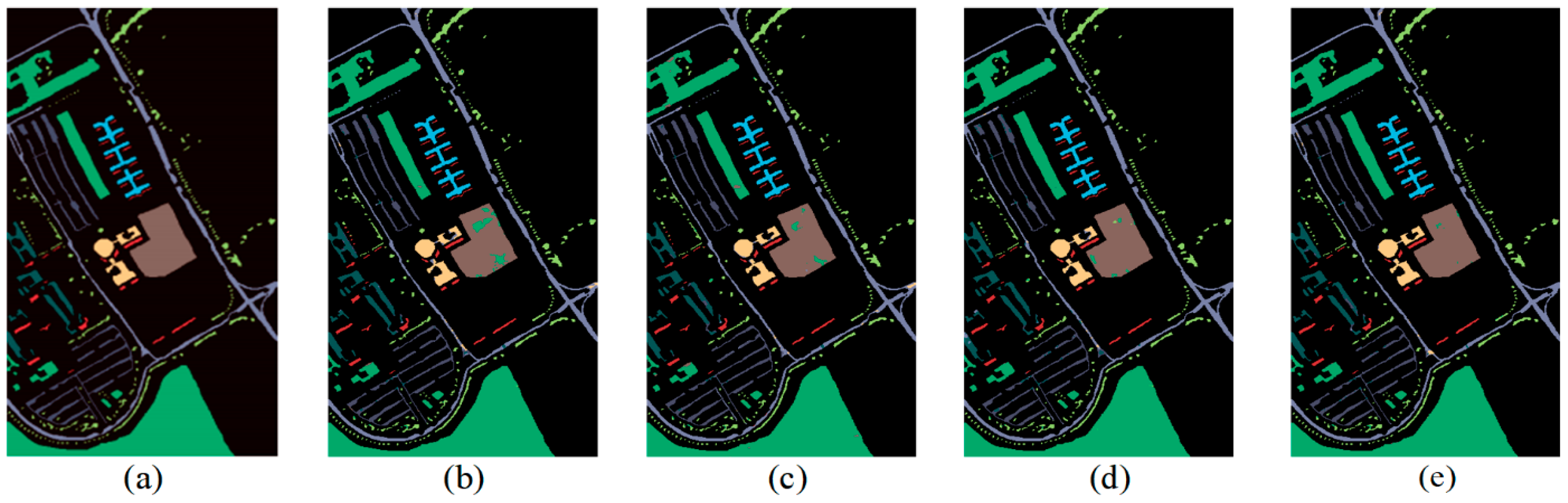
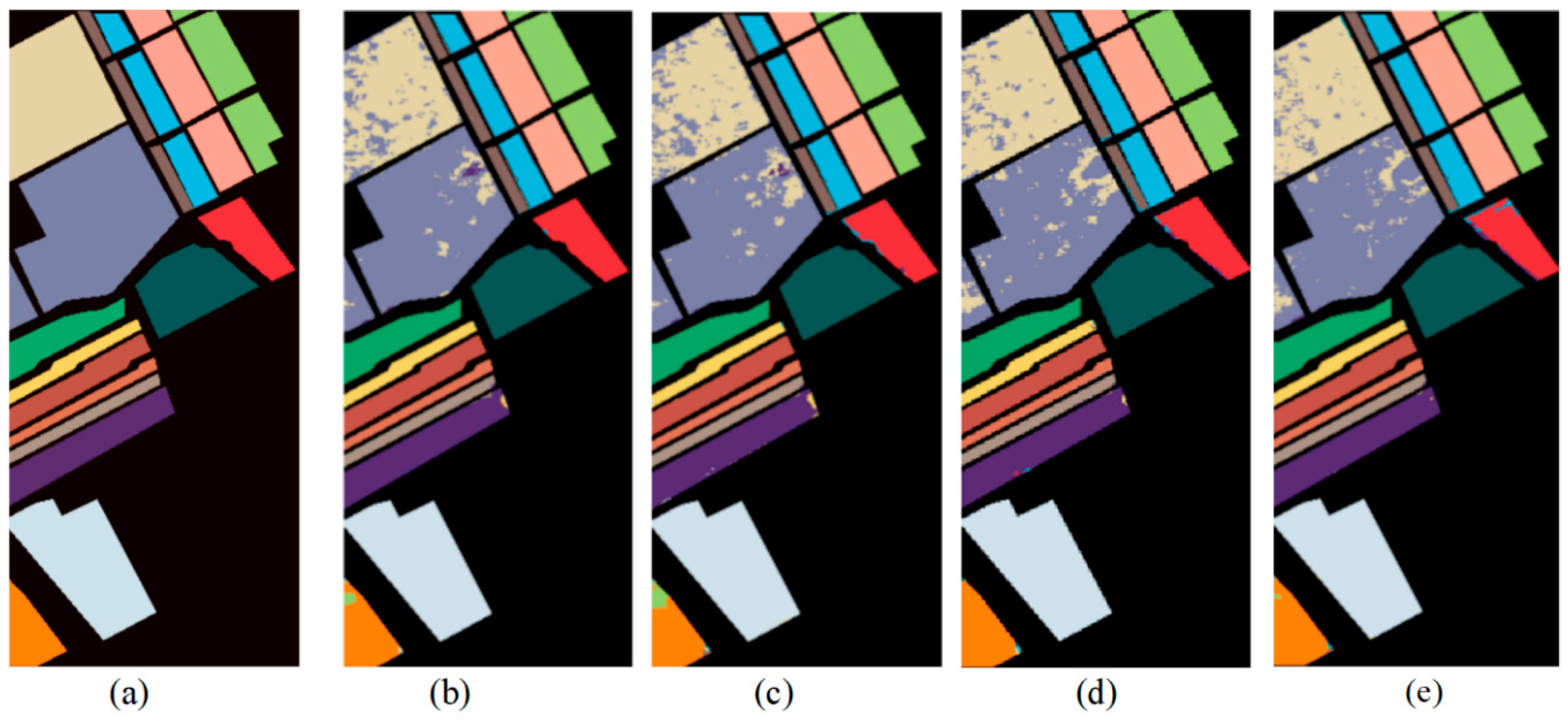
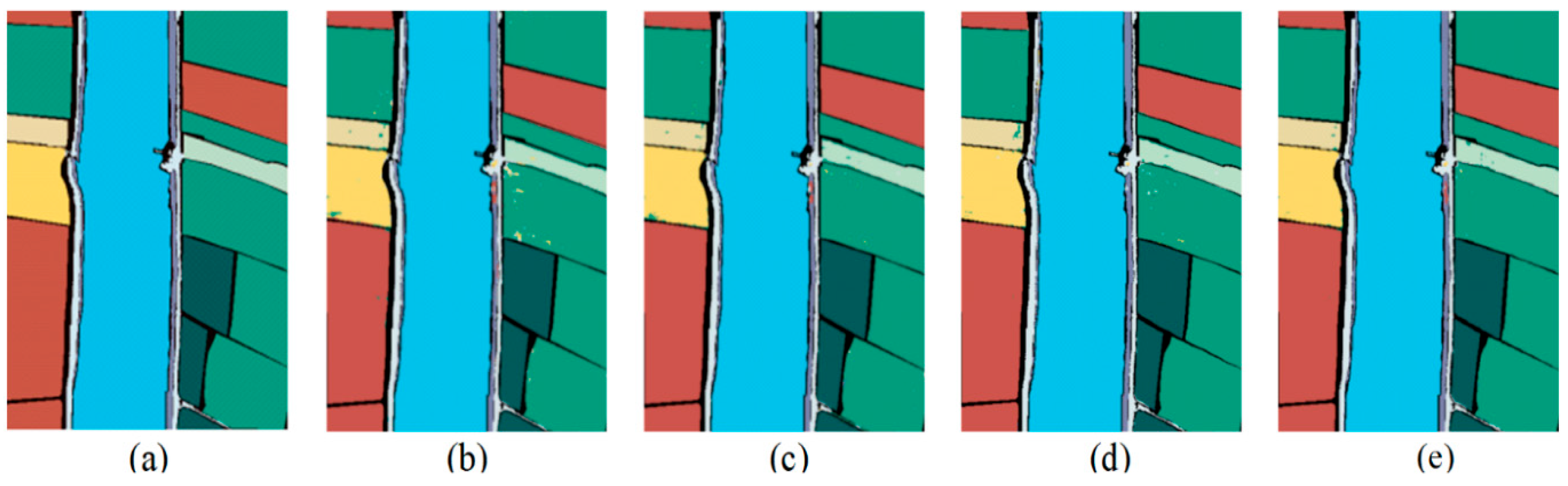
To validate the effectiveness of the proposed adaptive perception module and memory-guided mechanism, we conducted qualitative and quantitative evaluations of progressively enhanced network architectures. The qualitative results are presented in Figure 10, Figure 11, Figure 12 and Figure 13. Here, (a) denotes the ground truth. Our baseline, (b), consists of a two-layer convolutional encoder and a Transformer, forming the fundamental framework; (c), (d), and (e), respectively, represent the results obtained by gradually incorporating the single-sample globalization, batch internal globalization, and cross-batch globalization strategies. The quantitative metrics are summarized in

Table 11. Ablation experiment results.

Dataset	Metrics	Base Model	Single-Sample Globalization	Intra-Batch Globalization	Cross-Batch Globalization
PU	OA (%)	97.15 ± 0.28	97.25 ± 0.11	97.62 ± 0.21	98.00 ± 0.33
	AA (%)	95.19 ± 0.89	95.88 ± 0.78	96.33 ± 0.84	97.11 ± 0.13
	Kappa	96.22 ± 0.38	96.55 ± 0.41	96.84 ± 0.28	97.35 ± 0.44
SA	OA (%)	94.96 ± 0.27	95.15 ± 0.11	96.15 ± 0.37	96.21 ± 0.34
	AA (%)	97.15 ± 0.25	97.34 ± 0.37	97.82 ± 0.27	97.78 ± 0.45
	Kappa	94.38 ± 0.30	95.31 ± 0.32	95.71 ± 0.41	95.78 ± 0.38
WHU-LK	OA (%)	99.07 ± 0.19	99.13 ± 0.14	99.26 ± 0.13	99.32 ± 0.20
	AA (%)	97.03 ± 0.66	97.22 ± 0.45	97.31 ± 0.55	97.62 ± 0.71
	Kappa	98.77 ± 0.26	98.89 ± 0.10	99.03 ± 0.17	99.11 ± 0.26
KSC	OA (%)	87.39 ± 2.84	87.52 ± 1.87	88.68 ± 0.74	89.22 ± 0.91
	AA (%)	82.37 ± 2.27	82.56 ± 3.60	83.25 ± 2.66	83.43 ± 2.57
	Kappa	86.83 ± 3.63	87.14 ± 3.85	87.79 ± 2.54	87.93 ± 2.66

, where the bold indicates the best result.

Experimental findings demonstrate that the proposed adaptive perception module significantly enhances the model’s spatial adaptability, particularly improving its capacity to classify elongated or irregularly shaped land cover features. Using contextual information from neighboring pixels more effectively, the module substantially reduces misclassification errors for large-area land cover types. The incorporation of the memory-guided mechanism further enhances classification accuracy by aggregating spatial–spectral information from same-class samples across different batches. Finally, feature aggregation operation reinforces intra-class feature consistency while preserving inter-class boundaries, thereby generating more compact and well-separated feature embeddings.

4.2. Influencing Factor Analysis

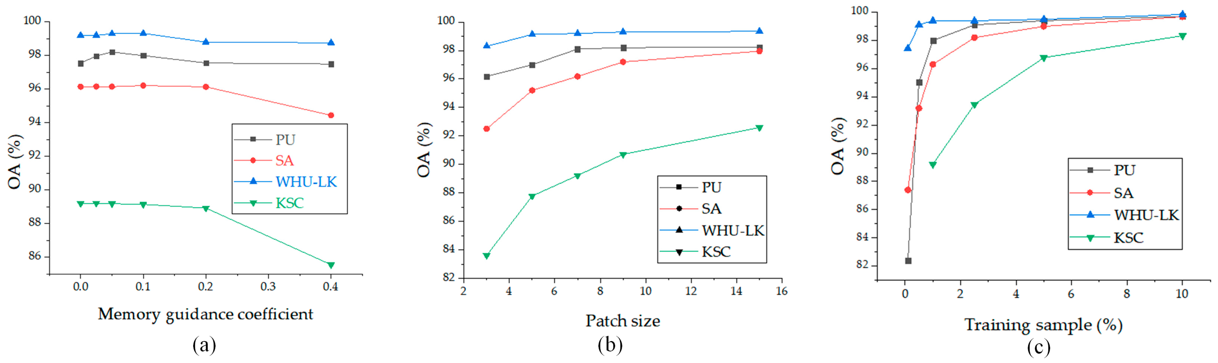
We conducted separate investigations into the impacts of the memory guidance coefficient, the patch size, and training samples on network classification performance. To analyze the effect of the memory guidance coefficient on overall classification accuracy, we configured the coefficient values as 0, 0.025, 0.05, 0.1, 0.2, and 0.4, with results illustrated in Figure 14a. The findings demonstrate that dataset-specific memory guidance coefficient settings are crucial for optimal performance. For the PU dataset, the optimal coefficient approximates 0.05, while values exceeding 0.2 for SA dataset and 0.1 for WHU-LK dataset would significantly degrade classification performance.

To evaluate the influence of patch size, we tested dimensions of 3 × 3, 5 × 5, 7 × 7, 9 × 9, and 15 × 15, as shown in Figure 14b. The overall classification accuracy exhibited an upward trend with increasing sample size, reaching peak performance at 15 × 15 within the tested range.

To evaluate the impact of training data quantity, we set proportions of total samples at 0.1%, 0.5%, 1%, 2.5%, 5%, and 10%, with outcomes depicted in Figure 14c. Considering that some classes in the KSC dataset would have had fewer than one training sample under the 0.1% and 0.5% proportions, we therefore started the evaluation on this dataset from 1%. Across all datasets, classification accuracy progressively improved with increased training samples, achieving maximum performance at 10% training proportion within the experimental configuration.

4.3. Limitations and Future Work

A limitation of the proposed approach is its reliance on a purely data-driven paradigm, which does not integrate a physical model. While this design offers flexibility and strong empirical performance, it lacks physical interpretability. The proposed adaptive perception Transformer is designed to adapt to the spatial morphology of input patches, but it lacks a corresponding adaptive mechanism for the spectral dimension. Extending the adaptive perception to jointly model spatial–spectral adaptivity represents a promising direction for future work.

Furthermore, the proposed method introduces computational overhead from two key components. On one hand, the memory-guided mechanism requires maintaining a dynamically updated memory bank and performing cross-batch feature retrieval, which increases both memory consumption and computational time. On the other hand, the adaptive perception Transformer adaptively modulates its attention based on the input patch, incurring additional computation beyond conventional Transformer blocks. Future work could explore the use of prototype-based strategies [56,57] to mitigate the computational overhead, alongside a comprehensive investigation into the trade-offs between performance and efficiency across various implementation strategies.

Beyond the design of classification networks and training strategies, the quality of input data is also critical. It fundamentally determines the upper bound of classification performance. Both the original and corrected versions of the KSC dataset are made available by the GIC of the UPV/EHU on its “Hyperspectral Remote Sensing Scenes” data repository. Preliminary experiments on this dataset demonstrate that, without altering the network architecture and training strategy, the corrected KSC dataset achieves nearly a 10% improvement in overall accuracy (OA) over the original dataset. In practice, hyperspectral data are inevitably corrupted by various types of noise. These include Gaussian noise, stripes, and water absorption interference. Spectral variability caused by illumination and atmospheric conditions also degrades the data. Therefore, effective preprocessing techniques such as denoising and correction [58,59,60] can improve spectral feature reliability and consequently potentially improve classification accuracy. This complementary perspective is also worth further investigation.

5. Conclusions

To address the performance limitations caused by small samples in hyperspectral image classification, this paper proposes MASSP, which integrates a three-level globalization strategy. Experimental results demonstrate that the proposed method consistently outperforms five competitive methods across all tested datasets. Specifically, using only 1% or fewer training samples, our method achieves outstanding overall accuracies of 96.15%, 97.81%, 89.22% and 99.32% on four public datasets. Furthermore, this paper systematically analyzes the impact of key factors, including the memory guidance coefficient, patch size, and training samples, on model performance. Future work will focus on targeted spectral analysis for challenging samples (e.g., broad-leaf vs. narrow-leaf soybeans, asphalt vs. bitumen, bare soil vs. meadows, and different grape field classes).

In future research, we plan to incorporate similarity metric mechanisms and attention mechanisms to enhance the network’s discriminative capability for challenging samples.

References

1. Wang, Y.; Xue, Z.; Jia, M.; Liu, Z.; Su, H. Hypergraph Convolutional Network with Multiple Hyperedges Fusion for Hyperspectral Image Classification Under Limited Samples. IEEE Trans. Geosci. Remote Sens. 2024, 62, 5526318. [Google Scholar] [CrossRef]
2. Morley, A.M.; Mather, T.A.; Pyle, D.M.; Kendall, J.M. Detecting Shallow Subsurface Anomalies with Airborne and Spaceborne Remote Sensing: A Review. Sci. Remote Sens. 2025, 11, 100187. [Google Scholar] [CrossRef]
3. Peng, L.; Xin, H.N.; Lv, C.X.; Li, N.; Li, Y.F.; Geng, Q.L.; Chen, S.H.; Lai, N. Inversion of Nitrogen and Phosphorus Contents in Cotton Leaves based on the Gaussian Mixture Model and Differences in Hyperspectral Features of UAV. Spectrochim. Acta Part A Mol. Biomol. Spectrosc. 2025, 327, 125419. [Google Scholar] [CrossRef] [PubMed]
4. Wu, Y.; Lu, C.; Wu, K.; Gao, W.; Yang, N.; Lin, J. Advancements and Trends in Mangrove Species Mapping based on Remote Sensing: A Comprehensive Review and Knowledge Visualization. Glob. Ecol. Conserv. 2025, 57, e03408. [Google Scholar] [CrossRef]
5. Yu, Y.; Xu, T.; Shen, Z.; Zhang, Y.; Wang, X. Compressive Spectral Imaging System for Soil Classification with Three-Dimensional Convolutional Neural Network. Opt. Express 2019, 27, 23029–23048. [Google Scholar] [CrossRef] [PubMed]
6. Sun, Q.; Chen, L.; Zhang, B.; Qu, X.; Cui, Y.; Shu, M.; Gu, X. Evaluation of Growth Recovery Grade in Lodging Maize via UAV-Based Hyperspectral Images. J. Remote Sens. 2024, 4, 0253. [Google Scholar] [CrossRef]
7. Lou, C.; Al-qaness, M.A.A.; Al-Alimi, D.; Dahou, A.; Abd Elaziz, M.; Abualigah, L.; Ewees, A.A. Land Use/Land Cover (LULC) Classification using Hyperspectral Images: A Review. Geo-Spat. Inf. Sci. 2024, 28, 345–386. [Google Scholar] [CrossRef]
8. Zhang, W.T.; Li, Y.B.; Liu, L.; Bai, Y.; Cui, J. Hyperspectral Image Classification Based on Spectral–Spatial Attention Tensor Network. IEEE Geosci. Remote Sens. Lett. 2024, 21, 5500305. [Google Scholar] [CrossRef]
9. Yu, C.; Zhu, Y.; Song, M.; Wang, Y.; Zhang, Q. Unseen Feature Extraction: Spatial Mapping Expansion with Spectral Compression Network for Hyperspectral Image Classification. IEEE Trans. Geosci. Remote Sens. 2024, 62, 5521915. [Google Scholar] [CrossRef]
10. Yang, H.; Yu, H.; Zheng, K.; Hu, J.; Tao, T.; Zhang, Q. Hyperspectral Image Classification based on Interactive Transformer and CNN with Multilevel Feature Fusion Network. IEEE Geosci. Remote Sens. Lett. 2023, 20, 5507905. [Google Scholar] [CrossRef]
11. Liu, Y.; Hao, A.; Liu, Y.; Liu, C.; Zhang, Z.; Cao, Y. Review of Hyperspectral Image Classification based on Deep Learning. Int. J. Pattern Recognit. Artif. Intell. 2024, 38, 2432001. [Google Scholar] [CrossRef]
12. Ding, H.; Liu, R.; Xiao, H.; Zeng, Q.; Liu, J.; Wang, Z.; Peng, Y.; Li, H. TBSSF-Net: Three-Branch Spatial-Spectral Fusion Network for Hyperspectral Image Classification. Opt. Express 2025, 33, 3466–3500. [Google Scholar] [CrossRef] [PubMed]
13. Chen, Y.; Zhao, X.; Jia, X. Spectral–Spatial Classification of Hyperspectral Data based on Deep Belief Network. IEEE J. Sel. Top. Appl. Earth Obs. Remote Sens. 2015, 8, 2381–2392. [Google Scholar] [CrossRef]
14. Chen, Y.; Lin, Z.; Zhao, X.; Wang, G.; Gu, Y. Deep Learning-Based Classification of Hyperspectral Data. IEEE J. Sel. Top. Appl. Earth Obs. Remote Sens. 2014, 7, 2094–2107. [Google Scholar] [CrossRef]
15. Mou, L.; Ghamisi, P.; Zhu, X.X. Deep Recurrent Neural Networks for Hyperspectral Image Classification. IEEE Trans. Geosci. Remote Sens. 2017, 55, 3639–3655. [Google Scholar] [CrossRef]
16. Zhang, X.; Sun, Y.; Jiang, K.; Li, C.; Jiao, L.; Zhou, H. Spatial Sequential Recurrent Neural Network for Hyperspectral Image Classification. IEEE J. Sel. Top. Appl. Earth Obs. Remote Sens. 2018, 11, 4141–4155. [Google Scholar] [CrossRef]
17. Huang, L.; Chen, Y. Dual-Path Siamese CNN for Hyperspectral Image Classification with Limited Training Samples. IEEE Geosci. Remote Sens. Lett. 2021, 18, 518–522. [Google Scholar] [CrossRef]
18. Yu, C.; Han, R.; Song, M.; Liu, C.; Chang, C.I. Feedback Attention-Based Dense CNN for Hyperspectral Image Classification. IEEE Trans. Geosci. Remote Sens. 2022, 60, 5501916. [Google Scholar] [CrossRef]
19. Ding, J.; Wei, W.; Zhang, L. Cross-Domain Distribution Calibration of Hyperspectral Image Classification. IEEE Geosci. Remote Sens. Lett. 2024, 21, 2503105. [Google Scholar] [CrossRef]
20. Zhang, H.; Ma, X.; Zhao, X.; Arce, G.R. Compressive Hyperspectral Image Classification using a 3D Coded Convolutional Neural Network. Opt. Express 2021, 29, 32875–32891. [Google Scholar] [CrossRef] [PubMed]
21. Liu, Q.; Peng, J.; Zhang, G.; Sun, W.; Du, Q. Deep Contrastive Learning Network for Small-Sample Hyperspectral Image Classification. J. Remote Sens. 2023, 3, 0025. [Google Scholar] [CrossRef]
22. Li, R.; Zheng, S.; Duan, C.; Wang, L.; Zhang, C. Land Cover Classification from Remote Sensing Images based on Multi-Scale Fully Convolutional Network. Geo-Spat. Inf. Sci. 2022, 25, 278–294. [Google Scholar] [CrossRef]
23. Wang, D.; Zhuang, L.; Gao, L.; Sun, X.; Zhao, X. Global Feature-Injected Blind-Spot Network for Hyperspectral Anomaly Detection. IEEE Geosci. Remote Sens. Lett. 2024, 21, 5509305. [Google Scholar] [CrossRef]
24. Hong, D.; Han, Z.; Yao, J.; Gao, L.; Zhang, B.; Plaza, A.; Chanussot, J. SpectralFormer: Rethinking Hyperspectral Image Classification with Transformers. IEEE Trans. Geosci. Remote Sens. 2022, 60, 5518615. [Google Scholar] [CrossRef]
25. Yu, H.; Xu, Z.; Zheng, K.; Hong, D.; Yang, H.; Song, M. MSTNet: A Multilevel Spectral–Spatial Transformer Network for Hyperspectral Image Classification. IEEE Trans. Geosci. Remote Sens. 2022, 60, 5532513. [Google Scholar] [CrossRef]
26. Zhou, H.; Zhang, X.; Zhang, C.; Ma, Q. Vision Transformer with Contrastive Learning for Hyperspectral Image Classification. IEEE Geosci. Remote Sens. Lett. 2023, 20, 5503905. [Google Scholar] [CrossRef]
27. Ahmad, M.; Ghous, U.; Usama, M.; Mazzara, M. WaveFormer: Spectral–Spatial Wavelet Transformer for Hyperspectral Image Classification. IEEE Geosci. Remote Sens. Lett. 2024, 21, 5502405. [Google Scholar] [CrossRef]
28. Arshad, T.; Zhang, J. Hierarchical Attention Transformer for Hyperspectral Image Classification. IEEE Geosci. Remote Sens. Lett. 2024, 21, 5504605. [Google Scholar] [CrossRef]
29. Jia, C.; Zhang, X.; Meng, H.; Xia, S.; Jiao, L. CenterFormer: A Center Spatial–Spectral Attention Transformer Network for Hyperspectral Image Classification. IEEE J. Sel. Top. Appl. Earth Obs. Remote Sens. 2025, 18, 5523–5539. [Google Scholar] [CrossRef]
30. Liao, J.; Wang, L. SSA-Mamba: Spatial-Spectral Attentive State Space Model for Hyperspectral Image Classification. IEEE J. Sel. Top. Appl. Earth Obs. Remote Sens. 2026, 19, 6403–6424. [Google Scholar] [CrossRef]
31. Yu, J.; Li, J.; Sun, G.; Lu, J.; Cheng, X.; Zhou, R.; Sun, W.; Gao, X. DualMambaFormer: A Parallel Hybrid Transformer–Mamba Network for Hyperspectral Image Classification. Remote Sens. 2026, 18, 1516. [Google Scholar] [CrossRef]
32. Xie, W.; Zhang, Y.; Sun, H.; Wu, Q. Hyperspectral Image Classification via 3D-CNN MHSA Fusion Transformer. In Proceedings of the 2023 IEEE International Geoscience and Remote Sensing Symposium (IGARSS 2023), Pasadena, CA, USA, 16–21 July 2023; pp. 7633–7636. [Google Scholar]
33. Wang, Z.; Li, Y.; Cheng, Z.; Zhang, Y. CNN and Transformer Hybrid Network for Hyperspectral Image Classification. In Proceedings of the 2024 IEEE International Geoscience and Remote Sensing Symposium (IGARSS 2024), Athens, Greece, 7–12 July 2024; pp. 9091–9095. [Google Scholar]
34. Mei, S.; Song, C.; Ma, M.; Xu, F. Hyperspectral Image Classification Using Group-Aware Hierarchical Transformer. IEEE Trans. Geosci. Remote Sens. 2022, 60, 5539014. [Google Scholar] [CrossRef]
35. Bian, T.; Yang, B.; Chen, Y.; Zhou, X.; Yue, L.; Hu, S. MDS3-Net: A Multiscale Spectral–Spatial Sequence Hybrid CNN–Transformer Model for Hyperspectral Image Classification. Remote Sens. 2026, 18, 977. [Google Scholar] [CrossRef]
36. Toker, K.G.; Yuksel, S.E. Spectral-Spatial Nearest Subspace Classifier for Hyperspectral Image Classification. Int. J. Remote Sens. 2022, 43, 2106–2133. [Google Scholar] [CrossRef]
37. Li, Z.; Guo, J.; Zhang, W.; Han, M.; Xu, Z.; Zhang, B.; Li, N.; Luo, W.; Xie, M.; Guo, J. CADR-BL: Class-Adaptive Dictionary Reconstruction with Broad Learning for Few-Shot Hyperspectral Image Classification. Remote Sens. 2026, 18, 1263. [Google Scholar] [CrossRef]
38. Zhang, C.; Yue, J.; Qin, Q. Deep Quadruplet Network for Hyperspectral Image Classification with a Small Number of Samples. Remote Sens. 2020, 12, 647. [Google Scholar] [CrossRef]
39. Pal, D.; Bundele, V.; Banerjee, B.; Jeppu, Y. SPN: Stable Prototypical Network for Few-Shot Learning-Based Hyperspectral Image Classification. IEEE Geosci. Remote Sens. Lett. 2022, 19, 5506905. [Google Scholar] [CrossRef]
40. Dong, S.; Quan, Y.; Feng, W.; Dauphin, G.; Gao, L.; Xing, M. A Pixel Cluster CNN and Spectral-Spatial Fusion Algorithm for Hyperspectral Image Classification with Small-Size Training Samples. IEEE J. Sel. Top. Appl. Earth Obs. Remote Sens. 2021, 14, 4101–4114. [Google Scholar] [CrossRef]
41. Zhang, B.; Chen, Y.; Xiong, S.; Lu, X. Hyperspectral Image Classification via Cascaded Spatial Cross-Attention Network. IEEE Trans. Image Process. 2025, 34, 899–913. [Google Scholar] [CrossRef] [PubMed]
42. Zhang, W.; Li, Z.; Zhen, T. Hybrid-KANet: A hyperspectral remote sensing crop classification method based on the Kolmogorov–Arnold network. Geo-Spat. Inf. Sci. 2025, 1–23. [Google Scholar] [CrossRef]
43. Liao, J.; Wang, L. ATN-Hybrid: A hybrid attention network with deterministic-probabilistic mechanism for hyperspectral image classification. Geo-Spat. Inf. Sci. 2025, 1–22. [Google Scholar] [CrossRef]
44. Hu, N.; Wang, Z.; Wang, M.; Zhao, Y. Double-Attention Context Interactive Network for Hyperspectral Image Classification. Remote Sens. 2026, 18, 1059. [Google Scholar] [CrossRef]
45. Zhang, Q.; Xiao, H.; Liu, J.; Shao, Z.; Wang, Z.; Peng, Y.; Li, H. Contextual interaction siamese network for few-shot hyperspectral image classification. Geo-Spat. Inf. Sci. 2026, 1–24. [Google Scholar] [CrossRef]
46. Li, K.; Liu, G.; Dang, M.; Wang, X. F2SNet: Frequency Feature Siamese Network for Few-Shot Hyperspectral Image Classification. In Proceedings of the 2025 IEEE International Geoscience and Remote Sensing Symposium (IGARSS 2025), Brisbane, Australia, 3–8 August 2025; pp. 2334–2338. [Google Scholar]
47. Xue, Z.; Zhou, Y.; Du, P. S3Net: Spectral–Spatial Siamese Network for Few-Shot Hyperspectral Image Classification. IEEE Trans. Geosci. Remote Sens. 2022, 60, 5531219. [Google Scholar] [CrossRef]
48. Wan, X.; Liu, H.; Chen, F.; Hu, K.; Li, Z. LFAH-Net: Laplacian Frequency Aware Hierarchical Network for Hyperspectral Image Classification. Digit. Signal Process. 2026, 168, 105561. [Google Scholar] [CrossRef]
49. Mei, S.; Li, X.; Liu, X.; Cai, H.; Du, Q. Hyperspectral Image Classification Using Attention-Based Bidirectional Long Short-Term Memory Network. IEEE Trans. Geosci. Remote Sens. 2022, 60, 5509612. [Google Scholar] [CrossRef]
50. Zhou, F.; Sun, X.; Sun, C.; Dong, J.; Zhu, X.X. Adaptive Morphology Filter: A Lightweight Module for Deep Hyperspectral Image Classification. IEEE Trans. Geosci. Remote Sens. 2023, 61, 5529316. [Google Scholar] [CrossRef]
51. Cao, C.; Xiang, H.; Song, W.; Yi, H.; Xiao, F.; Gao, X. Lightweight Multiscale Neural Architecture Search with Spectral–Spatial Attention for Hyperspectral Image Classification. IEEE Trans. Geosci. Remote Sens. 2023, 61, 5505315. [Google Scholar] [CrossRef]
52. Cui, Y.; Zhu, L.; Zhao, C.; Wang, L.; Gao, S. Lightweight Spectral–Spatial Feature Extraction Network based on Domain Generalization for Cross-Scene Hyperspectral Image Classification. IEEE Trans. Geosci. Remote Sens. 2024, 62, 5525514. [Google Scholar] [CrossRef]
53. Han, Z.; Yang, J.; Gao, L.; Zeng, Z.; Zhang, B.; Chanussot, J. Dual-Branch Subpixel-Guided Network for Hyperspectral Image Classification. IEEE Trans. Geosci. Remote Sens. 2024, 62, 5521813. [Google Scholar] [CrossRef]
54. Han, Z.; Yang, J.; Gao, L.; Zeng, Z.; Zhang, B.; Chanussot, J. Subpixel Spectral Variability Network for Hyperspectral Image Classification. IEEE Trans. Geosci. Remote Sens. 2025, 63, 5504014. [Google Scholar] [CrossRef]
55. Kong, L.; Sun, X.; Zhang, J.; Wang, X.; Shang, X. JDAWSL: Joint Domain Adaptation with Weight Self-Learning for Hyperspectral Few-Shot Classification. IEEE J. Sel. Top. Appl. Earth Obs. Remote Sens. 2025, 18, 21476–21493. [Google Scholar] [CrossRef]
56. Zhao, Z.; Kong, L.; Sun, X.; Wang, X.; Zhang, J.; Shang, X. FGAPA: Feature-Guided Adversarial Prototype Alignment For Cross-Domain Few-Shot Hyperspectral Classification. In Proceedings of the ICASSP 2026-2026 IEEE International Conference on Acoustics, Speech and Signal Processing (ICASSP), Barcelona, Spain, 3–8 May 2026; pp. 6216–6220. [Google Scholar]
57. Kong, L.; Sun, X.; Zhao, Z.; Zhang, J.; Shang, X. PGSMC: Prototype-Guided Supervised Momentum Contrastive Learning for Hyperspectral Cross-Domain Few-Shot Classification. IEEE Trans. Geosci. Remote Sens. 2025, 63, 5532918. [Google Scholar] [CrossRef]
58. Zhuang, L.; Ng, M.K.; Gao, L.; Wang, Z. Eigen-CNN: Eigenimages Plus Eigennoise Level Maps Guided Network for Hyperspectral Image Denoising. IEEE Trans. Geosci. Remote Sens. 2024, 62, 5512018. [Google Scholar] [CrossRef]
59. Han, J.; Pan, C.; Ding, H.; Zhang, Z. Double-Factor Tensor Cascaded-Rank Decomposition for Hyperspectral Image Denoising. Remote Sens. 2024, 16, 109. [Google Scholar] [CrossRef]
60. Zhang, Q.; Zheng, Y.; Yuan, Q.; Song, M.; Yu, H.; Xiao, Y. Hyperspectral Image Denoising: From Model-Driven, Data-Driven, to Model-Data-Driven. IEEE Trans. Neural Netw. Learn. Syst. 2024, 35, 13143–13163. [Google Scholar] [CrossRef] [PubMed]
Figure 1. Motivation of the proposed method.
Remotesensing 18 02225 g001
Figure 2. Overall architecture of Memory-Guided Adaptive Perception Transformer.
Remotesensing 18 02225 g002
Figure 3. Adaptive Perception Transformer.
Remotesensing 18 02225 g003
Figure 4. Memory-guided mechanism.
Remotesensing 18 02225 g004
Figure 5. The pseudocolor map and ground truth map of the HSI datasets. (a) PU; (b) SA; (c) WHU-LK; (d) KSC. The classes represented by the different colors in the ground truth map are listed in Table 2, Table 3 and Table 4.
Remotesensing 18 02225 g005
Figure 6. Classification results of the PU dataset: (a) ground truth; (b) AB-LSTM; (c) LMSS_NAS; (d) L-DGNet; (e) DSNet; (f) CSCANet; (g) JDAWSL; (h) proposed method.
Remotesensing 18 02225 g006
Figure 7. Classification results of the SA dataset: (a) ground truth; (b) AB-LSTM; (c) LMSS_NAS; (d) L-DGNet; (e) DSNet; (f) CSCANet; (g) JDAWSL; (h) proposed method.
Remotesensing 18 02225 g007
Figure 8. Classification results of the WHU-LK dataset: (a) hyperspectral false-color image; (b) ground truth; (c) ABLSTM; (d) LMSS; (e) L-DGNet; (f) DSNet; (g) CSCANet; (h) proposed method.
Remotesensing 18 02225 g008
Figure 9. Classification results of the KSC dataset: (a) ground truth; (b) AB-LSTM; (c) LMSS_NAS; (d) L-DGNet; (e) DSNet; (f) CSCANet; (g) JDAWSL; (h) proposed method.
Remotesensing 18 02225 g009
Figure 10. Classification results of the PU dataset: (a) ground truth; (b) baseline model; (c) single-sample globalization; (d) intra-batch globalization; (e) cross-batch globalization. The meanings of the different colors shown in the figure are provided in Table 2, Table 3 and Table 4.
Remotesensing 18 02225 g010
Figure 11. Classification results of the SA dataset: (a) ground truth; (b) baseline model; (c) single-sample globalization; (d) intra-batch globalization; (e) cross-batch globalization. The meanings of the different colors shown in the figure are provided in Table 2, Table 3 and Table 4.
Remotesensing 18 02225 g011
Figure 12. Classification results of the WHU-LK dataset: (a) ground truth; (b) baseline model; (c) single-sample globalization; (d) intra-batch globalization; (e) cross-batch globalization. The meanings of the different colors shown in the figure are provided in Table 2, Table 3 and Table 4.
Remotesensing 18 02225 g012
Figure 13. Classification results of the KSC dataset: (a) ground truth; (b) baseline model; (c) single-sample globalization; (d) intra-batch globalization; (e) cross-batch globalization. The meanings of the different colors shown in the figure are provided in Table 2, Table 3 and Table 4.
Remotesensing 18 02225 g013
Figure 14. Influencing factor analysis. (a) memory guidance coefficient; (b) patch size; (c) training samples.
Remotesensing 18 02225 g014