


Highlights
What are the main findings?
- Commercial vision-language models (VLMs; GPT-4o, GPT-5.5, Claude Sonnet 4.6) flagged harmful algal blooms with 73–93% false positive rates on bloom-absent satellite images, below the best RGB classifier and a trivial always-present baseline.
- The VLMs collapsed 60–70% of severity predictions into “moderate” regardless of actual conditions and identified at most one of the two severe blooms.
- A multi-spectral SVM (10 Sentinel-2 bands) achieved the strongest overall detection (F1 = 0.833, 79.5% accuracy, 27% false positive rate), outperforming every other method tested.
- Multi-spectral feature importances ranked the chlorophyll indices NDCI and Floating Algae Index among the top predictors, the same spectral signatures used in NOAA’s operational algorithms.
What are the implications of the main findings?
- The 12-percentage-point accuracy gain from RGB to multi-spectral features within the same SVM quantifies the spectral information gap, carried by the red-edge and shortwave infrared bands, that constrains RGB-only models and VLM vision encoders.
- For aquatic monitoring that requires spectral discrimination, domain-specific classifiers on multi-spectral data remain the right tool, and VLMs cannot substitute for them in spectral analysis.
- VLMs may serve a complementary role as narrative generators for non-specialist audiences, but their inability to access spectral bands is a hard boundary for current architectures.
Abstract
In recent years, there has been growing interest in applying vision–language models (VLMs) to quantitative remote sensing. This study evaluates whether three commercial VLMs (GPT-4o, GPT-5.5, and Claude Sonnet 4.6) can detect and classify the severity of harmful algal blooms (HABs) from Sentinel-2 satellite imagery of western Lake Erie and compares them against classical machine learning classifiers (Random Forest (RF), Support Vector Machine (SVM), and eXtreme Gradient Boosting (XGBoost)) trained on both a three-band red, green, blue (RGB) composite representation of the imagery and a 10-band multi-spectral reflectance representation. Forty bloom events identified from the National Oceanic and Atmospheric Administration (NOAA) Harmful Algal Bloom Operational Forecast System (HAB-OFS) severity assessments were assembled into the evaluation dataset, spanning seven bloom seasons (2019–2025). For binary bloom detection, the VLMs did not match the classical RGB classifiers; their F1 scores (0.69–0.75) fell below the best RGB classifier (Random Forest, 0.76) and below a trivial always-present baseline (F1 = 0.77), and they carried false positive rates of 73–93% on bloom-absent images, against 27–40% for the RGB classifiers. The VLMs reached high recall by labeling most scenes as bloom-positive, which makes them operationally unreliable in this configuration. For severity classification, the VLMs assigned 60–70% of their predictions to the “moderate” category regardless of actual conditions and identified at most one of the two severe blooms, whereas the classical classifiers tracked the ground-truth distribution and delivered two to nearly three times the exact-match accuracy (0.44–0.59 vs. 0.20–0.225). The strongest method across all metrics was the multi-spectral SVM (F1 = 0.833, false positive rate 27%, accuracy 0.795). Switching the same SVM from RGB to multi-spectral features raised accuracy from 0.675 to 0.795, a 12-percentage-point gain that measures the spectral information carried by red-edge and shortwave infrared bands that are accessible through multi-spectral sensors but unavailable to standard VLM vision encoders. Feature-importance analysis showed that the multi-spectral classifiers ranked chlorophyll-specific indices, the Normalized Difference Chlorophyll Index (NDCI) and the Floating Algae Index (FAI), among their top predictors, the same signatures used in established operational algorithms, while the RGB classifiers relied on red-channel variability and green-dominant pixel fractions because RGB inputs cannot compute those indices. Two compounded limitations therefore constrain off-the-shelf VLMs for aquatic remote sensing: the limited spectral information available through standard RGB channels and a mismatch between the land-dominated training distributions of these models and aquatic optical conditions. Domain-specific classifiers operating on multi-spectral data remain the more suitable tools for continued development of HAB monitoring and water-quality retrieval.
1. Introduction
Harmful algal blooms (HABs) are becoming a growing problem in eutrophied lakes and reservoirs globally. A series of observational studies over the last 30 years indicate that the frequency, duration and spatial extent of these events have all been increasing in response to both increasing levels of nutrients and warmer surface water temperatures [1,2,3,4]. The ecological impacts of cyanobacterial blooms extend far beyond the environment: a 2014 microcystin contamination event occurred when approximately 500,000 people had their drinking water supply shut down due to a massive toxic algae bloom occurring in Toledo, Ohio. This event exemplified the rapid transition from an ecological disaster to a public health crisis. Since then, satellite remote sensing has evolved as the primary surveillance mechanism for HAB events. Satellite remote sensing provides repeated basin-scale observations of water bodies that are impossible for in situ-based sampling mechanisms to provide [5,6].
Satellite-based HAB monitoring employs various types of operational systems that rely on the development of spectral algorithms tuned to the unique optical properties of photosynthetic pigments. For example, the National Oceanic and Atmospheric Administration (NOAA) Cyanobacteria Index (CI), which has been used operationally to monitor Lake Erie since 2009, utilizes the spectral shape around 681 nm to differentiate the chlorophyll-a fluorescence peak from other forms of background radiance [7]. Other algorithms include the Maximum Chlorophyll Index (MCI) and the Floating Algae Index (FAI), both of which utilize different spectral characteristics in the red-edge and near-infrared (NIR) regions of the spectrum [8,9]. Machine learning algorithms continue to advance the accuracy of detecting HABs using multi-spectral satellite imagery; recent research has shown that high-performing detectors can achieve F1 scores greater than 0.95 for Random Forest (RF) and Support Vector Machine (SVM) on Sentinel-2 imagery of eutrophic lakes [10], 91% detection accuracy for a convolutional neural network long short-term memory (CNN-LSTM) architecture on Florida coastal waters [11], and 87% overall accuracy for a one-class SVM applied to Lake Erie [12].
A separate trajectory in artificial intelligence, one largely disconnected from the remote sensing community until recently, has produced vision–language models (VLMs). VLMs can interpret natural images and return textual descriptions, classifications, or structured outputs. Models like GPT (OpenAI), Claude (Anthropic), and Gemini (Google) can now accept an image as input and answer questions about it. Tuia et al. [13] noted in their agenda-setting paper on AI for Earth sciences that the field risks falling into the trap of applying recent AI advances to well-resolved remote sensing problems rather than tackling genuinely hard scientific challenges. I ask whether these general-purpose models are being directed toward spectral classification tasks they were never intended to address.
The question has real-world urgency. In March 2025, Planet Labs and Anthropic announced a partnership to apply VLMs to satellite imagery analysis [14], signaling serious commercial investment in this space. Prior studies have evaluated VLMs on terrestrial remote sensing tasks such as land-use classification and change detection [15,16], and one 2024 study tested multimodal LLMs on hydrological applications using ground-level photographs [17]. However, no prior study has systematically evaluated VLM performance on satellite-derived aquatic imagery with the kind of controlled benchmarking required to determine whether VLMs can perform the task.
Watershed managers in resource-limited settings may be tempted to use VLMs simply because they do not require any remote sensing expertise to use: upload an image, get an answer. If that answer is wrong as often as 93% of the time for bloom-absent images, as this study demonstrates, the consequences are operational: unnecessary water quality advisories, wasted sampling campaigns, and eroded public trust.
This study addresses four research questions using a controlled benchmark on HAB detection within western Lake Erie.
- Can commercial VLMs detect bloom presence from Sentinel-2 red, green, blue (RGB) composites with accuracy comparable to classical machine learning (ML) classifiers trained on the same images (research question 1, RQ1)?
- Can commercial VLMs classify bloom severity on an ordinal scale, and does their classification behavior differ structurally from that of trained classifiers (RQ2)?
- How much does access to multi-spectral data (10 Sentinel-2 bands vs. three-band RGB) affect classifier performance, and what does this gap imply about the information available to VLMs (RQ3)?
- What are the dominant failure modes, including any that might be specific to the language-model architecture itself (RQ4)?
The experimental design compares VLMs and classical ML classifiers across three input configurations: VLMs on RGB composites, classifiers analyzing 33 features extracted from the same RGB composites, and classifiers analyzing 76 features from 10-band multi-spectral data. All methods are evaluated on the same 40 labeled HAB events using the same study area and evaluation protocol. To my knowledge, this is the first controlled comparison of VLMs against classical spectral classifiers for any aquatic remote sensing task and the first study to quantify the spectral information gap between RGB and multi-spectral inputs as a measured variable rather than an assumed limitation.
2. Related Work
2.1. Satellite Remote Sensing of Harmful Algal Blooms
The spectral basis for detecting cyanobacterial blooms from space is well established. Chlorophyll-a absorbs strongly at 440 nm (blue) and 675 nm (red) and fluoresces at approximately 681 nm. The spectral shape used by algorithms such as the CI enables separation of the cyanobacterial signal from the background water-leaving radiance [5,7,18]. The CI contains an inherent clear-water correction that suppresses false positives from optically shallow waters, a design feature whose significance becomes apparent when VLM performance is examined in Section 4.
Sentinel-2 is now the preferred sensor for inland water quality assessment at fine spatial scales. Its red-edge bands at 705, 740, and 783 nm (B05–B07) provide the spectral resolution needed for chlorophyll-a retrieval in optically complex waters [19,20], while the 10 m pixel size in the visible bands resolves nearshore variability that coarser sensors miss. The Normalized Difference Chlorophyll Index (NDCI), computed from the 705 nm red-edge and 665 nm red bands, has proven effective for chlorophyll-a estimation across diverse water body types [18,21]. The red-edge region is particularly important for cyanobacteria because it captures the reflectance shoulder near 705 nm, where cyanobacterial pigments produce a distinct spectral response that is distinguishable from eukaryotic algae, sediment, and colored dissolved organic matter (CDOM) [18,21]. Sensors limited to visible wavelengths do not have the capability to measure this region, nor do VLMs with only RGB inputs, as shown by this research.
The transition from the Medium Resolution Imaging Spectrometer (MERIS), decommissioned in 2012, to the Sentinel-3 Ocean and Land Colour Instrument (OLCI) maintained spectral continuity for large-lake HAB monitoring [22], while Sentinel-2 filled the spatial resolution gap for inland waters [19,20]. For Lake Erie, Stumpf et al. [23] built a long-term, satellite-derived biomass time series that NOAA uses for its annual Severity Index (SI), and validation of the CI across 11 U.S. states over 11 bloom seasons yielded overall accuracy between 77% and 87% [7].
2.2. Machine Learning for HAB Detection
Classical ML approaches have been tested on HAB detection across a range of water bodies and sensors. The reported accuracies are high when models operate on multi-spectral features: F1 values above 0.95 for Random Forest, eXtreme Gradient Boosting (XGBoost), and SVM on Sentinel-2 imagery of Chinese eutrophic lakes [10]; 87% overall accuracy for a one-class SVM on Lake Erie [12]; and 91% detection and 86% forecast accuracy for HABNet (CNN-LSTM) on Florida coastal Moderate Resolution Imaging Spectroradiometer (MODIS) datacubes [11]. Most recently, Joshi et al. [24] applied RF, Support Vector Regression (SVR), and XGBoost with SHapley Additive exPlanations (SHAP) explainability to predict chlorophyll-a concentration in the western Lake Erie basin using harmonized Landsat–Sentinel-2 imagery. They found that when they combined spectral bands with physicochemical variables, they were able to achieve an R-squared value of 0.76, but when utilizing spectral bands alone, the R-squared value dropped to 0.48.
What these benchmarks have in common is access to multi-band spectral data. Each classifier had access to all the band data provided by the sensor. This paper deliberately also tests classifiers on RGB-only features so that the comparison with VLMs, which are restricted to RGB input, is fair.
2.3. Vision–Language Models in Remote Sensing
Since 2023, VLM-based approaches for remote sensing have proliferated. RSGPT [15] and GeoChat [16] fine-tuned VLMs on terrestrial remote sensing imagery for scene classification, object detection, and captioning. Silva et al. [25] and Mall et al. [26] explored large language model (LLM)-based captioning and vision–language alignment for satellite imagery without requiring manual annotations, with the GRAFT framework demonstrating zero-shot classification and retrieval on remotely sensed data. These efforts have targeted land-cover and urban scenes almost exclusively.
However, aquatic applications of VLMs remain thin. Kadiyala et al. [17] tested four multimodal LLMs on hydrological tasks using ground-level photographs, including one algal bloom example, but their evaluation used in situ images rather than satellite data and included no quantitative comparison against established detection methods. No prior study has benchmarked VLMs on satellite-derived aquatic imagery against classical spectral classifiers under controlled conditions.
There are two architectural aspects of current VLMs that limit their applicability to spectral tasks. First, most VLM vision encoders, typically vision transformers pretrained on natural photographs, accept only three-channel RGB input. Second, most training data for these models consist overwhelmingly of terrestrial photographs, creating a domain gap for the optical properties of water.
Industry investment in VLMs for remote sensing is growing. The Planet–Anthropic partnership announced in March 2025 [14] signaled commercial commitment to this direction. Geospatial foundation models pretrained on satellite archives (Prithvi [27], Clay Foundation Model [28]) have shown promise for terrestrial transfer learning, raising parallel questions about generalization to aquatic domains. However, without evaluation data collected under controlled conditions, the remote sensing community cannot distinguish between productive applications and premature deployment. The present study provides that evaluation for one specific, operationally consequential task.
3. Materials and Methods
3.1. Study Area
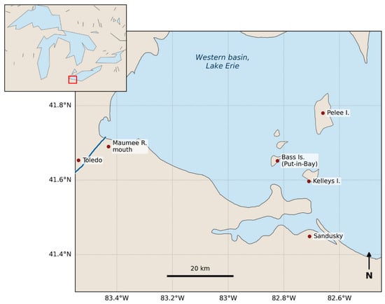
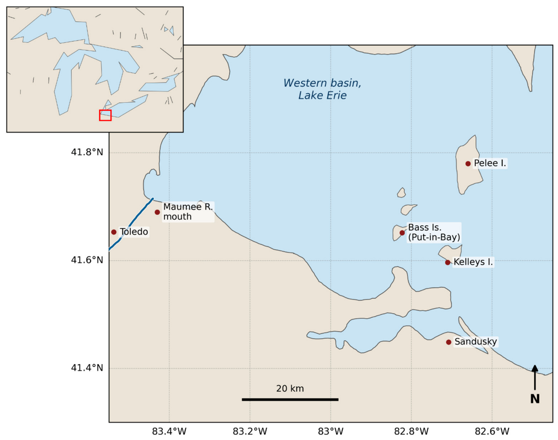
The western basin of Lake Erie (41.30–42.00°N, 83.55–82.45°W) was chosen for this study because it supports the most extensively monitored recurring cyanoHAB in North America (Figure 1). Annual Microcystis blooms, driven primarily by spring phosphorus loading from the Maumee River watershed, have been tracked by satellite remote sensing continuously since 2002 [7,23]. NOAA’s National Centers for Coastal Ocean Science (NCCOS) operate an HAB Operational Forecast System (HAB-OFS) that produces daily satellite-derived bloom assessments from June through November, providing a well-characterized ground-truth dataset against which new approaches can be tested.
Figure 1.
Study area: the western basin of Lake Erie (41.30–42.00°N, 83.55–82.45°W). The basin receives nutrient-laden runoff from the Maumee River watershed, producing annual Microcystis cyanobacterial blooms that have been monitored by the National Oceanic and Atmospheric Administration (NOAA) Harmful Algal Bloom Operational Forecast System (HAB-OFS) since 2002. Shoreline and river geometry are from the Global Self-consistent, Hierarchical, High-resolution Geography (GSHHG) and World Data Bank II (WDBII) databases.
3.2. Bloom Event Catalog
Forty bloom events from seven bloom seasons (2019–2025) were compiled into a single catalog representing the full range of observed severity across recent years. The seasons span a range of bloom magnitudes; reconciled NOAA Severity Index values, which capture peak 30-day mean cyanobacterial biomass on a 0–10 scale, were 5.9 (2019), 1.9 (2020), 3.4 (2021), 4.4 (2022), 2.9 (2023), 4.2 (2024), and 2.4 (2025).
Within each year, dates were distributed across five phenological phases that represent the development of a bloom: pre-bloom, early bloom, peak, late bloom, and post-bloom. Each date received both a binary bloom label (present/absent) and a four-level severity label (none/mild/moderate/severe) based on NOAA bulletin records and CI time series. The final catalog contained 15 “none,” 17 “mild,” 6 “moderate,” and 2 “severe” observations. The skew toward lower severity reflects bloom phenology: peak conditions exist during a smaller fraction of each season than developing or declining phases.
3.3. Satellite Data Acquisition
Sentinel-2 imagery was acquired through the Copernicus Data Space Ecosystem Sentinel Hub application programming interface (API). For each catalog date, the API was used to search a +/− 5-day window for the nearest cloud-free Sentinel-2 image (maximum 30% cloud cover, mosaicking set to least-cloudy scene).
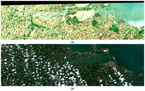
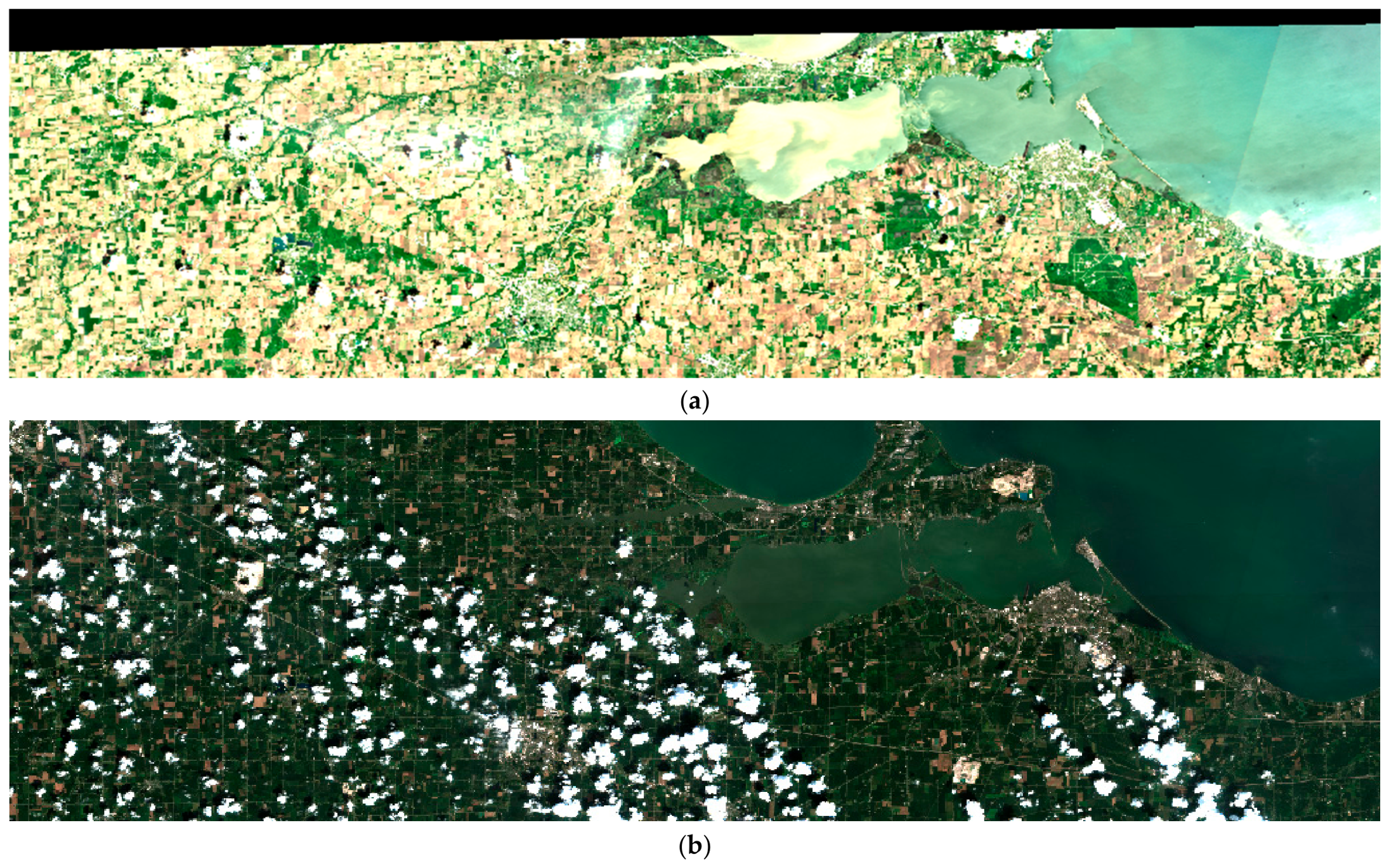
For each date, two products were generated. First, RGB composite images (B04/B03/B02 mapped to red/green/blue) were rendered as 1024 × 768 pixel PNGs. These served as VLM input and as the basis for RGB feature extraction. In these composites, algal blooms appear as green or blue-green discoloration against darker background water (Figure 2). Second, multi-spectral reflectance arrays of 10 Sentinel-2 Level-2A (L2A) bands (B02 through B08, B8A, B11, B12) were retrieved as calibrated surface reflectance at 512 × 384 pixels. All bands came from the Level-2A product, which provides bottom-of-atmosphere surface reflectance after Sen2Cor atmospheric correction, so no further atmospheric processing was applied. Because every method in this study, VLM and classifier, was evaluated on the same Level-2A reflectance, the choice of atmospheric correction shifts absolute reflectance uniformly across methods rather than changing their relative performance, which is the quantity this benchmark compares. This holds for a more basic reason as well: atmospheric correction rescales bands the sensor already measured but cannot supply bands that the RGB mapping leaves out. The red-edge and shortwave infrared reflectance that separates the multi-spectral classifiers from the RGB methods stays unavailable under any correction, so the central comparison rests on which bands each method can read, not on how those bands were corrected. The 60 m atmospheric bands (B01, B09, B10) were excluded.
Figure 2.
(a) Example Sentinel-2 true-color composites of the western Lake Erie basin pre-bloom conditions (15 June 2019): the water appears dark with tan-brown sediment plumes extending from the mouth of the Maumee River, the class of scene that produced the highest vision–language model (VLM) false positive rates. (b) Example Sentinel-2 true-color composites of the western Lake Erie basin peak bloom conditions (20 August 2021): green discoloration from cyanobacteria is visible across the western basin, concentrated near the shoreline and extending past the Bass Islands. Both images were used in the VLM evaluation.
One date (10 August 2023) yielded no usable multi-spectral data due to persistent cloud cover, reducing the multi-spectral dataset to 39 images.
3.4. Feature Extraction
3.4.1. Water Masking
For RGB composites, a heuristic mask excluded pixels with mean brightness below 0.02 (shadow/no-data) or above 0.7 (cloud/land), as well as pixels where red exceeded 50% of the total signal. For multi-spectral data, the Normalized Difference Water Index (NDWI = (B03 − B08)/(B03 + B08)) [29] was computed, with pixels above −0.1 classified as water. The brightness bounds remove dark shadow and no-data pixels and bright cloud or land pixels, the red-fraction test suppresses sediment-dominated and exposed-shoreline pixels, and the NDWI threshold separates open water from land and clouds in the multi-spectral arrays. Both masks required at least 100 valid water pixels per scene so that per-scene statistics rested on a sufficient water sample.
3.4.2. RGB Features (33 Features)
From each masked composite, 33 features were extracted: channel statistics (mean, standard deviation, median, and 10th and 90th percentiles for R, G, B; 15 features), spectral ratios (green/red, green/blue, blue/red ratios, green fraction, and Normalized Green–Red Difference Index (NGRDI) [30]; 12 features), and spatial features (green-dominant fraction, high-green fraction, brightness statistics, and Excess Green Index [31]; 6 features).
3.4.3. Multi-Spectral Features (76 Features)
From each masked 10-band array, 76 features were extracted. Per-band statistics (mean, standard deviation, 10th percentile, median, and 90th percentile for each of 10 bands) produced 50 features. Six established aquatic spectral indices were computed: Normalized Difference Vegetation Index (NDVI) [32] = (B08 − B04)/(B08 + B04), NDCI = (B05 − B04)/(B05 + B04), NDWI = (B03 − B08)/(B03 + B08), FAI = B08 − B04 − (B11 − B04) × (842 − 665)/(1610 − 665), MCI = B06 − B05 − 0.5 × (B07 − B05), and CI = B05 − 0.5 × (B04 + B06). The mean, standard deviation, and 90th percentile of each index were retained (18 features). Band ratios (B05/B04, B03/B02, B04/B03, B08/B04, and B11/B08) and two spatial threshold features (fraction of pixels with CI > 0.001 and fraction with NDCI > 0.05) completed the set.
3.5. VLM Evaluation Protocol
Three commercial VLMs were evaluated: GPT-4o (OpenAI), GPT-5.5 (OpenAI), and Claude Sonnet 4.6 (Anthropic). All accept image inputs through their APIs and return text responses, and the evaluation was run in June 2026. GPT-4o was retired from the ChatGPT consumer application in February 2026 but remains available through the OpenAI API, which allowed its evaluation on the same catalog. To reduce stochastic variation between runs, GPT-5.5 was run with reasoning effort set to none and a fixed random seed; GPT-4o and Claude Sonnet 4.6 expose no reasoning-effort control, and Claude Sonnet 4.6 used a low sampling temperature.
Each model performed two tasks. In Task A (binary detection), the model received a single Sentinel-2 RGB composite and was asked whether a harmful algal bloom was present. The model returned a structured JavaScript Object Notation (JSON) response with a Boolean bloom_present field, a confidence level (high/medium/low), and a reasoning string explaining the visual cues behind the classification. In Task B (severity classification), the model used the same RGB composite to classify bloom severity on a four-level ordinal scale (none/mild/moderate/severe), with descriptive criteria for each level provided in the prompt.
The evaluation tested four prompt strategies, organized as a progression from minimal to maximal guidance. The logic behind this progression is that each successive strategy provides additional information that a human analyst might bring to the task, and the question at each step is whether the VLM can use the additional information to improve its classification accuracy.
The first strategy, zero-shot, provides no domain context. The model receives only the image and the question (“Is there a harmful algal bloom present?”), relying entirely on whatever knowledge its pretraining encoded about satellite imagery, water bodies, and algal blooms. This establishes a performance floor.
The second strategy, zero-shot with context, identifies the image as a Sentinel-2 composite of western Lake Erie and describes the typical visual characteristics of cyanobacterial blooms (green or blue-green discoloration, surface scum patterns). The question here is whether naming the sensor, the location, and the target phenomenon narrows the model’s interpretive space enough to improve accuracy.
The third strategy, few-shot, adds textual descriptions of what bloom-present and bloom-absent images look like, including distinguishing features (color, texture, spatial distribution). No actual image examples were provided. The question is whether verbal exemplars help calibrate the model’s visual assessment without visual examples.
The fourth strategy, chain-of-thought, instructs the model to analyze the image step by step: first describe the overall water color, then identify any green or blue-green areas, then consider whether discoloration could be sediment rather than algae, and only then make a classification. The hypothesis is that forcing explicit reasoning about alternative explanations (sediment vs. algae) might reduce the false positive rate by making the model confront the distinction it might have otherwise glossed over.
Each combination of model, task, strategy, and image was evaluated in three independent repeats, yielding 2880 API calls (3 models × 40 dates × 2 tasks × 4 strategies × 3 repeats). Of these, 2844 (98.75%) returned valid JSON. For every image, the three repeats were aggregated to a single prediction by majority vote, with ties broken toward the lower class, and the reported VLM results use the per-image majority vote.
3.6. Classical ML Evaluation Protocol
Three machine learning classifiers were tested: Random Forest (100 trees, max depth 5), SVM with a radial basis function (RBF) kernel (C = 10, gamma = scale), and XGBoost (100 trees, max depth 4, learning rate 0.1). All of them used class-weighted training to compensate for the imbalanced severity distribution. Each classifier was trained on both the 33-feature RGB set and the 76-feature multi-spectral set for Tasks A and B. Features were standardized (zero mean, unit variance) using training-set statistics.
Cross-validation used a leave-one-year-out (LOYO) protocol: for each of the seven years, the classifier was trained on the other six years (32–35 samples) and tested on the held-out year (5–8 samples). This temporal separation prevents overfitting due to within-season autocorrelation and simulates the real-world scenario of deploying a model trained on historical blooms to a new season.
3.7. Evaluation Metrics
Model performance is evaluated with several metrics.
For Task A, I report accuracy, precision, recall, F1 score, and false positive rate (FPR = FP/(FP + TN), where FP is the number of false positives and TN the number of true negatives). FPR is reported as a separate metric because it captures a failure mode with direct operational consequences; false bloom alerts trigger water quality advisories, emergency sampling, and beach closures that consume limited resources and degrade public trust [33].
For Task B, I report exact-match accuracy, within-one accuracy (prediction within one ordinal step of truth), and severity mean absolute error (MAE, ordinal scale 0–3). Prediction distributions across severity categories were compared against the ground truth to reveal systematic biases.
4. Results
4.1. Task A: Binary Bloom Detection
Table 1 reports binary detection performance across all methods. VLM results reflect the best-F1 prompt strategy per model (chain-of-thought for GPT-4o and Claude Sonnet 4.6, zero-shot with context for GPT-5.5).
Table 1.
Binary harmful algal bloom (HAB) detection performance (Task A).
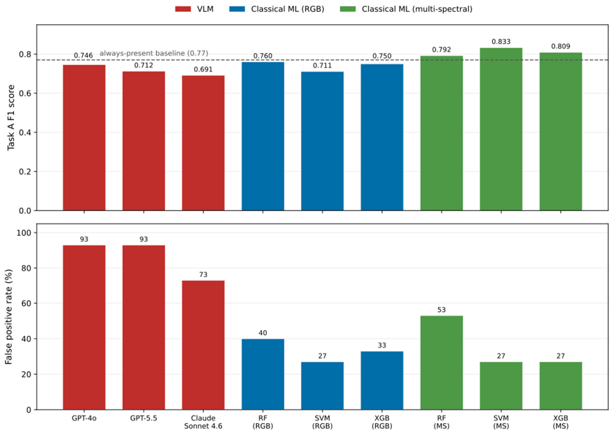
Across the RGB-input methods, the three VLMs did not lead on F1. GPT-4o scored 0.746, GPT-5.5 scored 0.712, and Claude Sonnet 4.6 scored 0.691, all below the best RGB classifier, Random Forest at 0.760, and below the F1 of a trivial always-present baseline (0.769), which labels every scene as a bloom. GPT-4o’s score is over 38 images, as two of its chain-of-thought responses did not parse. The VLMs reached these scores through high recall, 0.96 for GPT-4o, 0.84 for GPT-5.5, and 0.76 for Claude, by classifying most scenes as bloom-positive. That behavior produced false positive rates of 93% for GPT-4o, 93% for GPT-5.5, and 73% for Claude on the bloom-absent images. The three RGB classifiers were more balanced, with false positive rates between 27% and 40% (SVM 27%, XGBoost 33%, Random Forest 40%) at comparable or higher F1 values. The three RGB classifiers are nonetheless distinct models; their confusion matrices (Table 2) place detection errors differently, with false positives ranging from four (SVM) to six (Random Forest) and false negatives from six (Random Forest) to nine (SVM).
Table 2.
Confusion matrices for binary bloom detection (Task A) for the three classifiers trained on red, green, blue (RGB) features over the 40 events (25 bloom-present, 15 bloom-absent). Counts are true positives (TP; bloom-present → bloom-present), false negatives (FN; bloom-present → bloom-absent), false positives (FP; bloom-absent → bloom-present), and true negatives (TN; bloom-absent → bloom-absent). The three classifiers place errors differently, confirming they are distinct models despite the similar summary metrics in Table 1.
The multi-spectral SVM gave the strongest detection of any method: F1 of 0.833, accuracy of 0.795, and a false positive rate of 27%. Switching the same SVM algorithm from RGB to multi-spectral features raised accuracy from 0.675 to 0.795 and F1 from 0.711 to 0.833, a 12-percentage-point accuracy gain. The false positive rate stayed at 27%, so the multi-spectral bands improved overall accuracy and recall balance rather than reducing the false positive rate relative to the RGB SVM.
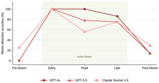
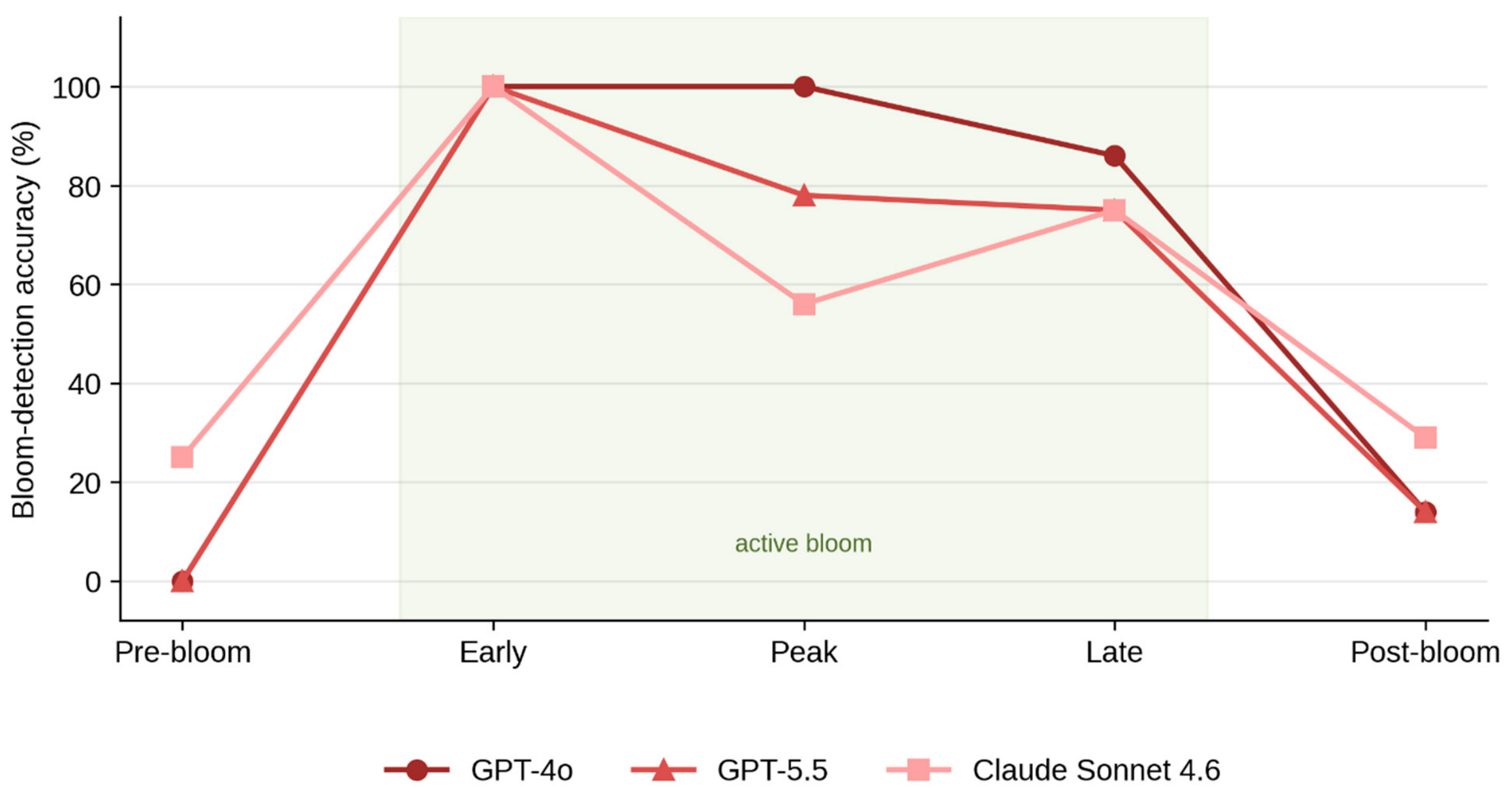
Performance also varied with bloom phenology (Figure 3). All three VLMs detected early-phase blooms with perfect accuracy (100%), when green discoloration stands out against pre-season water. The failures concentrated at the season margins, where the correct answer is “no bloom”; for pre-bloom images GPT-4o and GPT-5.5 correctly identified 0% and Claude Sonnet 4.6 identified 25%, and for post-bloom images GPT-4o and GPT-5.5 reached 14% and Claude 29%. GPT-4o held higher accuracy through the peak (100%) and late (86%) phases, while GPT-5.5 and Claude fell between the extremes (56–78%). The classifiers did not show this phase-dependent collapse, which is consistent with their lower overall false positive rates in Table 1.
Figure 3.
Bloom-detection accuracy by phenological phase (Task A) for each VLM at its best-F1 prompt strategy. All three models reached 100% accuracy in the early-bloom phase but misclassified most pre-bloom and post-bloom scenes as bloom-positive; GPT-4o and GPT-5.5 correctly identified 0% of pre-bloom images. The shaded band marks the active-bloom phases (early, peak, late).
Examining the VLM reasoning strings for false positives revealed a consistent misdiagnosis. On a pre-bloom image from 20 June 2020, with no bloom present, GPT-5.5 classified the scene as a bloom with high confidence and wrote: “A large green to yellow-green discoloration is visible in the western basin near the Maumee River plume, spreading offshore. This color and location are consistent with a Microcystis harmful algal bloom rather than normal deep-water color or clouds.” The image showed an early-season plume from the Maumee River. Suspended sediment produces green-brown turbidity that resembles early algal discoloration in true-color composites but has a completely different spectral signature in the red-edge and shortwave infrared (SWIR) bands, which the VLM cannot access.
4.2. Task B: Severity Classification
Table 3 reports severity classification performance across all methods.
Table 3.
Severity classification performance (Task B). VLM results reflect the best exact-match prompt strategy per model (zero-shot with context for GPT-4o, chain-of-thought for GPT-5.5, few-shot for Claude Sonnet 4.6). Mod. Bias = fraction of predictions assigned to “moderate”.
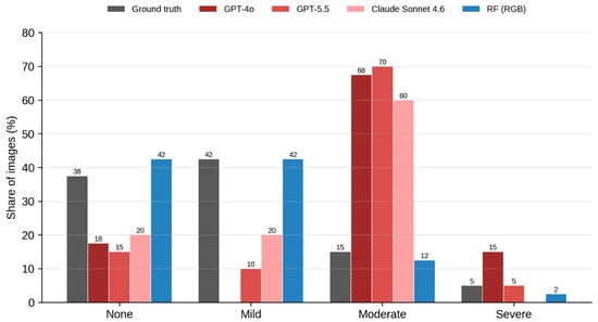
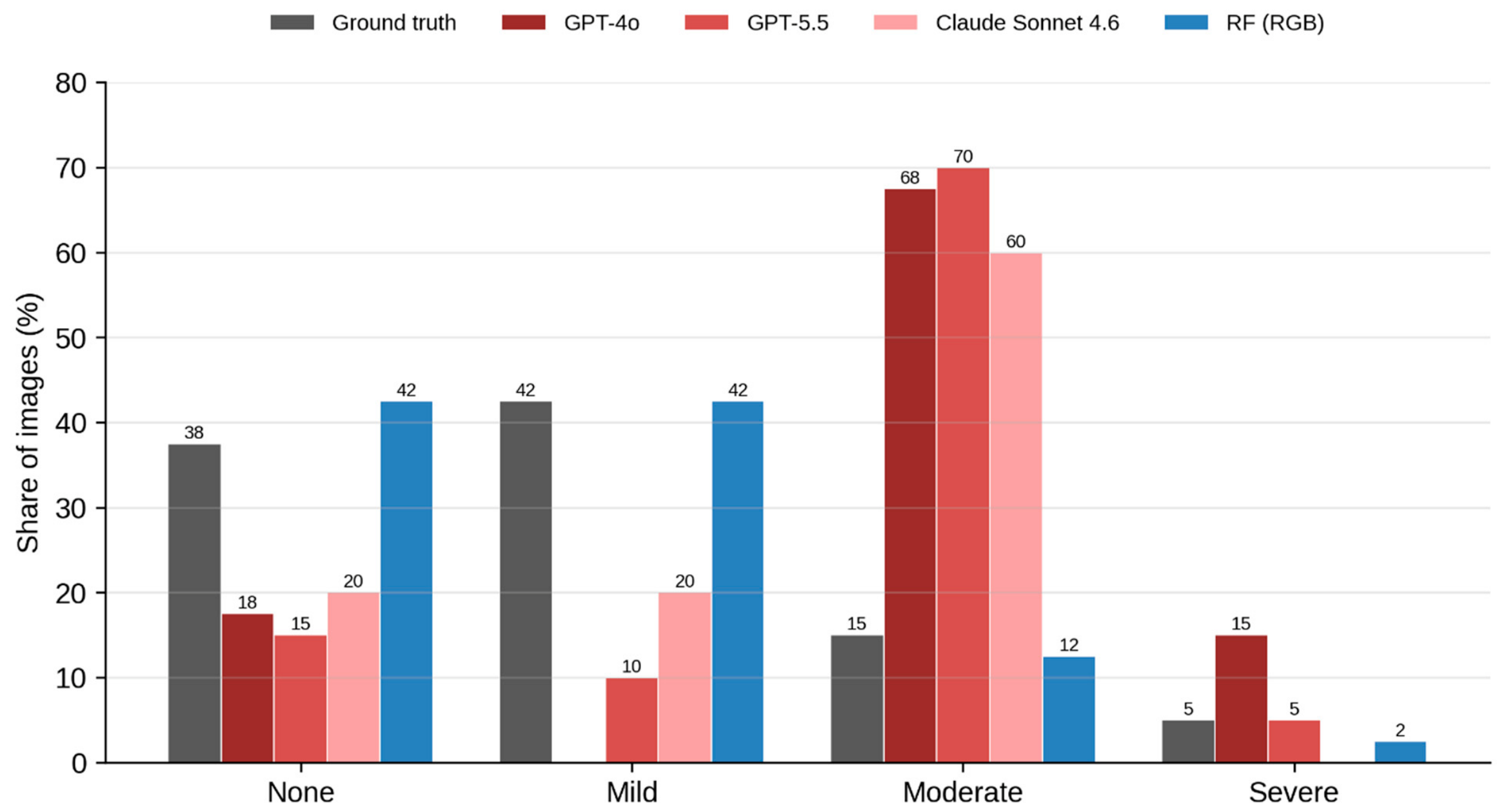
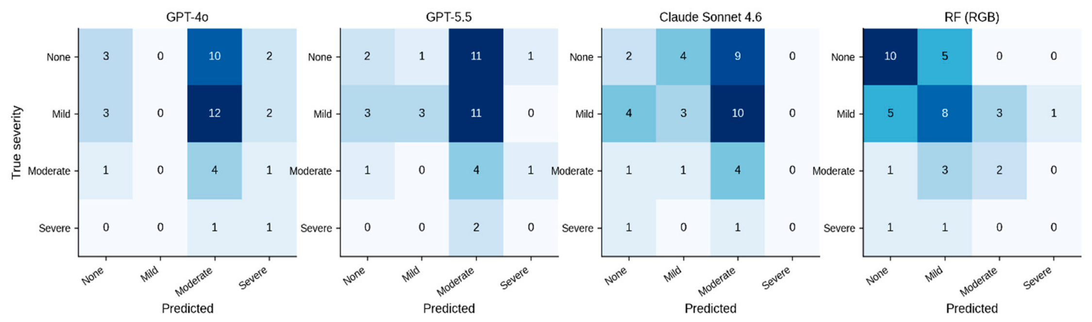
The severity results exposed a behavioral pattern that the classical ML results did not show. The ground truth was distributed as 37.5% none, 42.5% mild, 15% moderate, and 5% severe. GPT-4o assigned 68% of its severity predictions to “moderate,” GPT-5.5 assigned 70%, and Claude Sonnet 4.6 assigned 60% (Figure 4). GPT-5.5 and Claude Sonnet 4.6 identified none of the two “severe” blooms (0% recall for the severe class), while GPT-4o identified one of the two, as the confusion matrices in Figure 5 show.
Figure 4.
Severity prediction distribution across methods compared to ground truth (Task B). The VLMs collapsed 60–70% of predictions into the “moderate” category regardless of actual conditions, while the classical classifiers produced distributions that tracked the ground-truth proportions. Random Forest on RGB features most closely matched the true distribution.
Figure 5.
Confusion matrices for severity classification (Task B): GPT-4o, GPT-5.5, Claude Sonnet 4.6, and Random Forest on RGB features. Rows are true severity; columns are predicted severity. All three VLMs concentrated predictions in the “moderate” column across true severity levels; GPT-5.5 and Claude gave 0% recall for the “severe” class while GPT-4o identified one of the two severe blooms, and the Random Forest distributed predictions along the diagonal.
The classical ML classifiers, on RGB or multi-spectral features, produced prediction distributions that tracked the ground truth. Random Forest on RGB features predicted 42.5% none, 42.5% mild, 12.5% moderate, and 2.5% severe, close to the true proportions. Exact-match accuracy for the classifiers ranged from 0.44 to 0.59, roughly double the VLM values of 0.20 to 0.225.
Multi-spectral features did not consistently improve severity classification over RGB features: exact-match accuracy was 0.50 for all three RGB classifiers, against 0.487 (RF), 0.436 (SVM), and 0.590 (XGBoost) on multi-spectral features. With 40 samples and only two labeled “severe,” the four-class severity task is constrained by label scarcity more than by spectral information.
4.3. Prompt Strategy Effects
Adding domain context, verbal examples, and chain-of-thought instructions produced only small changes in Task A F1 values: the range across the four strategies was 0.721 to 0.746 for GPT-4o, 0.690 to 0.712 for GPT-5.5, and 0.667 to 0.691 for Claude Sonnet 4.6. The “moderate” bias in Task B persisted across all four strategies and all three models, which rules out prompt design as the cause. The bias appears to be structural, originating in the model rather than the prompt.
4.4. Feature Importance
Table 4 reports the top five features for binary bloom detection by input type.
Table 4.
Top five features for binary bloom detection by input type (Random Forest, full dataset training).
4.5. Confidence Calibration
The two feature sets describe different routes to a bloom decision. The RGB classifiers relied most on the fraction of green-dominant pixels and on red-channel variability (red_p90, red_mean, red_std) together with the green–red index (NGRDI). These are rough proxies; green dominance correlates with chlorophyll, and high red variability correlates with the spectral heterogeneity that blooms introduce. The multi-spectral classifiers ranked chlorophyll-specific indices, the elevated-pixel fraction and 90th percentile of NDCI and the mean Floating Algae Index, at the top, alongside the SWIR/NIR band ratio. These are close to the spectral signatures that NOAA’s operational CI exploits [7]. Because the ground-truth labels themselves derive from a CI-based assessment, a multi-spectral classifier learning CI-like features is partly expected and partly circular; the result indicates that the model recovered the spectral structure used to define the labels rather than independently rediscovering bio-optical theory.
Confidence calibration differed sharply across model generations. GPT-4o, the earlier-generation model, reported “high” confidence on 97% of its responses, including images it misclassified, committing almost every call at high confidence. GPT-5.5 reported “high” on only 18% of its responses, “medium” on 69%, and “low” on 13%, so it rarely committed to a high-confidence call. Claude Sonnet 4.6 fell between them, reporting “high” on 45% of responses, again with little relationship between its confidence ratings and actual accuracy. A monitoring system that reports high confidence on wrong answers is worse than one that reports no confidence at all because it suppresses the skepticism that human operators would otherwise bring to an uncertain result.
5. Discussion
5.1. The Spectral Information Bottleneck
When the same SVM algorithm with the same hyperparameters was run on RGB features (accuracy 0.675) and then on multi-spectral features (accuracy 0.795), the only variable that changed was the input data (Figure 6). The 12-point accuracy gain reflects the additional information carried by the seven extra spectral bands. The red-edge bands at 705–783 nm span the steep rise in pigment and vegetation reflectance between roughly 680 and 750 nm; this region is distinct from the broader near-infrared and carries far more than chlorophyll fluorescence alone, including the reflectance shoulder and pigment-absorption features that help separate algal pigments from sediment scattering [18,21]. The near-infrared bands beyond the red-edge and the shortwave infrared band at 1610 nm add further discrimination, with the SWIR capturing scattering properties that vary with particle type. These multi-spectral features are correlated, so dimensionality-reduction or band-selection methods such as principal component analysis or recursive feature elimination could compress them into a smaller operational set without losing the red-edge and SWIR information that drives the accuracy gain; the full feature set was used here to characterize the available information rather than to optimize a deployed model. The false positive rate of the multi-spectral SVM (27%) matched that of the RGB SVM, so the spectral bands improved overall accuracy rather than the false positive rate at this sample size. Without these bands, every method tested, VLM or classifier, struggled to separate green water caused by algae from green water caused by suspended sediment.
Figure 6.
Task A performance across the three method families: vision–language models, classical machine learning (ML) on RGB features, and classical ML on multi-spectral features. The top panel shows F1 scores with the always-present baseline (F1 = 0.77) marked; the bottom panel shows the false positive rates on bloom-absent images. The multi-spectral Support Vector Machine (SVM) gave the strongest overall detection (F1 = 0.833, 27% false positive rate, accuracy 0.795). The VLMs sat below the always-present F1 baseline and carried the highest false positive rates.
VLMs face this bottleneck in its most constrained form. Their vision encoders accept a (height, width, 3) tensor and nothing else. False-color composites or index-enhanced visualizations can be provided as alternative RGB mappings, but they still compress multi-band information into three visual channels, discarding the quantitative spectral relationships that operational algorithms depend on [7,8].
5.2. The “Moderate Collapse” and Language Model Training
When asked to classify bloom severity on an ordinal scale, all three VLMs defaulted to “moderate” between 60% and 70% of the time. No prompt strategy corrected this, and the pattern held across all four prompts and all three models, which points to a cause upstream of the prompt. One plausible contributor is the reinforcement learning from human feedback (RLHF) process [34] that shapes VLM behavior, though the present data show an association rather than a demonstrated mechanism.
Language models are trained to produce responses that human evaluators rate favorably, and in conversational settings hedged, moderate responses often receive higher ratings than extreme claims. For ordinal classification of environmental conditions, a preference of this kind could push predictions toward the scale center. Classical ML classifiers optimize cross-entropy or hinge loss, which penalizes all misclassifications equally and carries no preference for any particular output category, and class weighting further counteracts majority-class bias. Consistent with this, the classifiers tracked the ground-truth distribution while the VLMs did not, although the benchmark cannot isolate RLHF from other differences between the model families. Alternative explanations include a central-tendency or anchoring bias toward the middle of an ordinal scale and training priors in which intermediate severity descriptions are more frequent than extreme ones. Distinguishing these from an RLHF effect would require a controlled test, for example, comparing a base model against its RLHF-tuned counterpart on the same severity task or varying the scale framing to see whether the central category continues to attract predictions.
5.3. The False Positive Problem
From an operational point of view, the false positive rates are the most consequential finding. Each false positive can trigger a water quality advisory, a beach closure, or an emergency sampling deployment. Over time, high false positive rates erode the credibility of the monitoring system itself [33].
The cause is identifiable in the VLM reasoning strings. All three models interpreted sediment plumes, river-mouth turbidity, and CDOM-colored water as algal signatures. In the western Lake Erie basin, spring sediment loads from the Maumee River routinely produce green-brown water that, in a three-channel composite, looks much like an early bloom. The CI algorithm separates these visually similar conditions using spectral-shape tests around the fluorescence peak [7]. VLMs, limited to pattern-matching on RGB images, have no access to the spectral features that make this discrimination possible.
The contrast in false positive rates is between the VLMs and the classifiers, not between RGB and multi-spectral inputs. The RGB and multi-spectral SVMs both held the false positive rate at 27%, while the VLMs ran at 73% and 93%. The binding difference is therefore the modeling approach applied to RGB scenes, with the VLMs labeling most images as bloom-positive, rather than spectral access alone. Comparing an RGB VLM directly against a multi-spectral SVM conflates two differences, the model family and the input bands, and is not a clean model-level comparison; the two controlled contrasts in this study are VLM versus classifier on identical RGB inputs, which isolates the model, and SVM on RGB versus multi-spectral inputs, which isolates the spectral information.
5.4. Where VLMs Do and Do Not Add Value
Each VLM prediction came with an explanation of the visual reasoning behind it. These explanations were frequently wrong in their conclusions, but they described the image content in ways that a probability score or SVM decision value cannot: “green discoloration concentrated near the western shoreline, spreading toward the Bass Islands.” For watershed managers without remote sensing training, that description is more actionable than “P(bloom) = 0.73.”
A hybrid architecture that combines classical ML for detection with VLMs for narrative generation could use this division of labor. The classifier handles the spectral discrimination that requires band-level data, and a VLM, conditioned on the classifier output and the source image, translates the result into a description that non-specialists can act on.
This result should not be read as a verdict against VLMs in environmental monitoring; it is a statement about task fit. Quantitative bloom detection from calibrated reflectance is a narrow, well-posed classification problem, the kind of task a small, cheap, well-trained classical model handles reliably. Asking a general-purpose VLM to do this work, on three-band composites that discard the bands the task depends on, applies the most expensive tool available to a job a lighter one does better. Multi-purpose generative models draw orders of magnitude more energy per query than task-specific classifiers [35], so this mismatch spends disproportionate energy on work a lighter model does more accurately, at odds with the conservation goal the monitoring is meant to serve. The useful question is not whether VLMs can replace classical detectors, but which parts of a monitoring workflow genuinely fit them. Their value appears where the classical models are silent: turning a detection into a plain-language description a manager can act on, reasoning over heterogeneous inputs such as bulletins and field notes alongside imagery, and operating zero-shot on a new site or a rare event where no labeled training set exists yet.
That framing also indicates where the technology could move. A VLM trained or adapted on multi-band remote sensing data, rather than on the three-channel photographs that current vision encoders expect, would remove the input bottleneck this study identifies and could combine spectral discrimination with language-based reasoning in one model. Until such models exist and are validated, the practical way to place a VLM in an operational pipeline is to match each task to the lightest capable tool: keep quantitative detection with the classical classifiers, which deliver it accurately and at far lower computational cost, and call on the foundation model for the interpretation, synthesis, and triage steps where its flexibility justifies the added cost.
5.5. Off-the-Shelf vs. Fine-Tuned VLMs: What Training Can and Cannot Fix
Fine-tuning could address the training distribution mismatch. Off-the-shelf VLMs confuse sediment with algae because their vision encoders were trained on natural photographs where green water is meaningless. A VLM fine-tuned on labeled satellite composites of bloom, sediment, CDOM, and clear-water conditions could learn the visual distinctions that currently defeat these models. Fine-tuned remote sensing VLMs like RSGPT [15] and GeoChat [16] have shown this for terrestrial tasks.
Fine-tuning cannot address the spectral bottleneck. A fine-tuned VLM still receives three-channel RGB input. Even when a VLM is trained on labeled data to separate blooms, sediment, and similar conditions from RGB, the red-edge reflectance shoulder near 705 nm and the SWIR scattering signature at 1610 nm remain absent from the input. The 33 features extractable from RGB and the 76 features from 10-band data occupy fundamentally different information spaces. No training procedure applied to the former recovers the discriminative content of the latter. The constraint is architectural: it lives in the (height, width, 3) input tensor shape, and only structural changes to the vision encoder pipeline can remove it.
Multi-spectral foundation models like Prithvi [27] and Clay [28] do accept multi-band inputs natively, bypassing the three-channel limit. However, they lack the language generation capability that makes VLMs appealing for interpretive reporting. A future architecture combining a multi-spectral encoder with a language decoder could, in principle, close both gaps, though no such system has been demonstrated for aquatic applications.
There is also a practical paradox. The accessibility that makes VLMs attractive to resource-limited organizations—no training data needed, no graphics processing unit (GPU) infrastructure, no ML expertise, etc.—evaporates once fine-tuning enters the picture. Collecting labeled datasets, running training jobs, and validating the result demand the same workflow as building a classical classifier, but with the added overhead of a billion-parameter model. These resources would likely be better spent training a multi-spectral SVM that can access the discriminative spectral bands.
5.6. Implications for Watershed Remote Sensing
Spectral band access should be treated as a prerequisite for AI-based water quality monitoring, not an optional upgrade. The 12-point accuracy gap between the RGB and multi-spectral SVM applies well beyond HAB detection to chlorophyll-a retrieval, CDOM mapping, and trophic state assessment of lakes and reservoirs. All of these rely heavily on the spectral information available in red-edge and SWIR bands [18,20,21].
The false positive rate deserves equal consideration along with accuracy and F1 values in evaluation protocols for new monitoring tools. A system that achieves high recall by labeling everything as bloom-positive may look competitive on F1 while generating constant false alarms that drain response budgets and erode institutional trust [33].
The “moderate collapse” observed in severity classification should serve as a warning for any application of language-model-based AI to ordinal environmental scales. Drought severity, water quality grades, habitat condition scores, and wildfire danger ratings all use ordinal classifications where the trained tendency toward hedged responses could produce the same distributional compression documented here. Researchers applying VLMs to these tasks should report prediction distributions, not just summary accuracy metrics.
5.7. Limitations
The sample size (40 images, two severe observations) is small by ML standards, so the comparisons here rest on effect sizes and consistency across models rather than on statistical significance; at this size, none of the pairwise differences would be expected to reach significance. LOYO cross-validation with 32–35 training samples per fold limits all classifiers, and the similar performance across RF, SVM, and XGBoost on RGB features suggests training-data volume is the binding constraint for the RGB condition.
Only true-color RGB composites were tested as VLM input. False-color composites might improve VLM performance by making algal signatures more visually distinct, though they still compress multi-band information into three channels.
Two VLMs were evaluated at a single point in time (May 2026). VLM capabilities are improving rapidly, and future models trained on remote sensing data or those capable of processing multi-channel inputs may perform differently.
Ground-truth labels derive from NOAA’s CI-based operational assessments, so classifiers that learn CI-like features are partly learning to replicate the labeling algorithm. The labels are also scene-level: each image carries a single bloom and severity label, which is a proxy for the pixel-level spatial extent of a bloom. The bloom-absent scenes were drawn from clear and unambiguous cases, so the classifier specificity reported here is likely optimistic for the harder boundary conditions, such as sediment plumes and mixed water, that an operational system would face. Validation against in situ chlorophyll-a and microcystin measurements, and against pixel-level bloom maps, would provide a stronger basis for evaluating the VLMs and the classifiers. The results also come from a single, well-characterized site. The western basin of Lake Erie is dominated by Microcystis and by sediment loading from one major river, so the error rates reported here may not transfer to reservoirs, estuaries, or coastal waters with different optical properties, bloom-forming taxa, and background constituents. Moreover, operational HAB monitoring needs spatial bloom extent, intensity gradients, and time-series continuity, which the scene-level metrics used here (accuracy, F1, false positive rate, exact-match accuracy, and severity MAE) do not capture; these metrics screen a method rather than establish operational readiness. Finally, all methods were evaluated on Sen2Cor Level-2A reflectance without an inland-water-specific atmospheric correction; this affects every method equally and so does not change the relative comparison, but an inland-water correction such as ACOLITE or C2RCC could shift absolute performance and is worth testing in future work.
6. Conclusions
When tested on the same 40 bloom events from the same study area using the same evaluation protocol, commercial VLMs and classical ML classifiers produced different results. The VLMs did not lead on binary detection; GPT-4o (F1 = 0.746), GPT-5.5 (F1 = 0.712), and Claude Sonnet 4.6 (F1 = 0.691) fell below the best RGB classifier (Random Forest, F1 = 0.760) and below an always-present baseline (F1 = 0.77), and they classified 73–93% of bloom-absent images as bloom-positive. Classical ML on the same RGB data was more balanced (false positive rates of 27–40%), and the multi-spectral SVM outperformed every other method (F1 = 0.833, false positive rate 27%, accuracy 0.795).
For severity classification, the three VLMs predicted “moderate” for 60–70% of images regardless of actual conditions and identified at most one of the two severe blooms. The classical classifiers reached roughly double the exact-match accuracy and produced prediction distributions that tracked the ground truth. The severity bias is consistent with the hedging behavior associated with RLHF training and was not addressable through prompt engineering, though the benchmark cannot establish RLHF as the sole cause.
The 12-percentage-point accuracy gap between the RGB SVM and the multi-spectral SVM (0.675 vs. 0.795) measures the spectral information carried by the red-edge and SWIR bands that VLM vision encoders cannot access. Random Forest feature importance showed that the most discriminative multi-spectral features are chlorophyll indices, the Normalized Difference Chlorophyll Index and the Floating Algae Index, that align with the signatures used in NOAA’s operational monitoring; the RGB classifiers, which cannot compute these indices, instead relied on red-channel and green-dominance proxies.
For aquatic monitoring tasks that require spectral discrimination, domain-specific classifiers on multi-spectral satellite data remain the right tool. VLMs may serve a complementary role as narrative generators for non-specialist audiences, but they cannot substitute classical ML classifiers for spectral analysis. As VLMs continue to enter remote sensing workflows through commercial partnerships and accessible APIs, the community should evaluate them with controlled experimental designs that separate spectral information content from model architecture. The spectral demands of aquatic remote sensing represent a hard boundary that current VLM architectures cannot cross.
Supplementary Materials
The following supporting information can be downloaded at: https://www.mdpi.com/article/10.3390/rs18132147/s1.
Funding
This research received no external funding.
Data Availability Statement
Sentinel-2 L2A imagery was accessed through the Copernicus Data Space Ecosystem https://dataspace.copernicus.eu/ (accessed on 30 June 2026). NOAA HAB-OFS severity assessments and seasonal bulletins are available from NOAA NCCOS https://coastalscience.noaa.gov/science-areas/habs/hab-forecasts/lake-erie/ (accessed on 30 June 2026). The evaluation code, prompt templates, and per-sample model outputs are provided as Supplementary Materials. All result tables and figures, including the per-classifier confusion matrices, are contained within this article.
Acknowledgments
I thank the anonymous reviewers and the editors for their insightful comments and constructive suggestions, which improved the quality of this manuscript.
Conflicts of Interest
The author declares no conflict of interest.
Abbreviations
The following abbreviations are used in this manuscript:
| AI | Artificial Intelligence |
| API | Application Programming Interface |
| CDOM | Colored Dissolved Organic Matter |
| CI | Cyanobacteria Index |
| CNN | Convolutional Neural Network |
| FAI | Floating Algae Index |
| FN | False Negative |
| FP | False Positive |
| FPR | False Positive Rate |
| GPU | Graphics Processing Unit |
| HAB | Harmful Algal Bloom |
| HAB-OFS | Harmful Algal Bloom Operational Forecast System |
| JSON | JavaScript Object Notation |
| L2A | Level 2A (Sentinel-2 processing level) |
| LLM | Large Language Model |
| LOYO | Leave-One-Year-Out |
| LSTM | Long Short-Term Memory |
| MAE | Mean Absolute Error |
| MCI | Maximum Chlorophyll Index |
| MERIS | Medium Resolution Imaging Spectrometer |
| ML | Machine Learning |
| MODIS | Moderate Resolution Imaging Spectroradiometer |
| NCCOS | National Centers for Coastal Ocean Science |
| NDCI | Normalized Difference Chlorophyll Index |
| NDVI | Normalized Difference Vegetation Index |
| NDWI | Normalized Difference Water Index |
| NGRDI | Normalized Green–Red Difference Index |
| NIR | Near-Infrared |
| NOAA | National Oceanic and Atmospheric Administration |
| OLCI | Ocean and Land Colour Instrument |
| RBF | Radial Basis Function |
| RF | Random Forest |
| RGB | Red, Green, Blue |
| RLHF | Reinforcement Learning from Human Feedback |
| RQ | Research Question |
| SHAP | SHapley Additive exPlanations |
| SI | Severity Index |
| SVM | Support Vector Machine |
| SVR | Support Vector Regression |
| SWIR | Shortwave Infrared |
| TN | True Negative |
| TP | True Positive |
| VLM | Vision–Language Model |
| XGBoost | eXtreme Gradient Boosting |
References
- Paerl, H.W.; Huisman, J. Blooms like it hot: Climate change and harmful algal blooms. Science 2008, 320, 57–58. [Google Scholar] [CrossRef] [Scilit] [PubMed]
- Chorus, I.; Welker, M. (Eds.) Toxic Cyanobacteria in Water, 2nd ed.; World Health Organization: Geneva, Switzerland, 2021. [Google Scholar]
- Ho, J.C.; Michalak, A.M.; Pahlevan, N. Widespread global increase in intense lake phytoplankton blooms since the 1980s. Nature 2019, 574, 667–670. [Google Scholar] [CrossRef] [Scilit] [PubMed]
- Huisman, J.; Codd, G.A.; Paerl, H.W.; Ibelings, B.W.; Verspagen, J.M.H.; Visser, P.M. Cyanobacterial blooms. Nat. Rev. Microbiol. 2018, 16, 471–483. [Google Scholar] [CrossRef] [Scilit] [PubMed]
- Kutser, T.; Metsamaa, L.; Strombeck, N.; Vahtmae, E. Monitoring cyanobacterial blooms by satellite remote sensing. Estuar. Coast. Shelf Sci. 2006, 67, 303–312. [Google Scholar] [CrossRef] [Scilit]
- Palmer, S.C.J.; Kutser, T.; Hunter, P.D. Remote sensing of inland waters: Challenges, progress and future directions. Remote Sens. Environ. 2015, 157, 1–8. [Google Scholar] [CrossRef] [Scilit]
- Lunetta, R.S.; Schaeffer, B.A.; Stumpf, R.P.; Keith, D.; Jacobs, S.A.; Murphy, M.S. Evaluation of cyanobacteria cell count detection derived from MERIS imagery across the eastern USA. Remote Sens. Environ. 2015, 157, 24–34. [Google Scholar] [CrossRef] [Scilit]
- Gower, J.; King, S.; Borstad, G.; Brown, L. Detection of intense plankton blooms using the 709 nm band of the MERIS imaging spectrometer. Int. J. Remote Sens. 2005, 26, 2005–2012. [Google Scholar] [CrossRef] [Scilit]
- Hu, C. A novel ocean color index to detect floating algae in the global oceans. Remote Sens. Environ. 2009, 113, 2118–2129. [Google Scholar] [CrossRef] [Scilit]
- Yang, C.; Tan, Z.; Li, Y.; Shen, M.; Duan, H. A comparative analysis of machine learning methods for algal bloom detection using remote sensing images. IEEE J. Sel. Top. Appl. Earth Obs. Remote Sens. 2023, 16, 7953–7967. [Google Scholar] [CrossRef] [Scilit]
- Hill, P.R.; Kumar, A.; Temimi, M.; Bull, D.R. HABNet: Machine learning, remote sensing-based detection of harmful algal blooms. IEEE J. Sel. Top. Appl. Earth Obs. Remote Sens. 2020, 13, 3229–3239. [Google Scholar] [CrossRef] [Scilit]
- Ananias, P.H.M.; Negri, R.G. Anomalous behaviour detection using one-class support vector machine and remote sensing images: A case study of algal bloom occurrence in inland waters. Int. J. Digit. Earth 2021, 14, 921–942. [Google Scholar] [CrossRef] [Scilit]
- Tuia, D.; Roscher, R.; Wegner, J.D.; Jacobs, N.; Zhu, X.X.; Camps-Valls, G. Toward a collective agenda on AI for earth science data analysis. IEEE Geosci. Remote Sens. Mag. 2021, 9, 88–104. [Google Scholar] [CrossRef] [Scilit]
- Planet Labs; Anthropic. Planet and Anthropic Partnership for Geospatial AI. Press Release. March 2025. Available online: https://investors.planet.com/news/news-details/2025/Planet-and-Anthropic-Partner-to-Use-Claudes-Advanced-AI-Capabilities-to-Turn-Geospatial-Satellite-Imagery-into-Actionable-Insights/default.aspx (accessed on 30 June 2026).
- Hu, Y.; Yuan, J.; Wen, C.; Lu, X.; Li, X. RSGPT: A remote sensing vision language model and benchmark. arXiv 2023, arXiv:2307.15266. [Google Scholar] [CrossRef] [Scilit]
- Kuckreja, K.; Danish, M.S.; Naseer, M.; Das, A.; Khan, S.; Khan, F.S. GeoChat: Grounded large vision-language model for remote sensing. arXiv 2023, arXiv:2311.15826. [Google Scholar] [CrossRef] [Scilit]
- Kadiyala, L.A.; Mermer, O.; Samuel, D.J.; Sermet, Y.; Demir, I. The Implementation of Multimodal Large Language Models for Hydrological Applications: A Comparative Study of GPT-4 Vision, Gemini, LLaVa, and Multimodal-GPT. Hydrology 2024, 11, 148. [Google Scholar] [CrossRef] [Scilit]
- Mishra, S.; Mishra, D.R. Normalized difference chlorophyll index: A novel model for remote estimation of chlorophyll-a concentration in turbid productive waters. Remote Sens. Environ. 2012, 117, 394–406. [Google Scholar] [CrossRef] [Scilit]
- Toming, K.; Kutser, T.; Laas, A.; Sepp, M.; Paavel, B.; Noges, T. First experiences in mapping lake water quality parameters with Sentinel-2 MSI imagery. Remote Sens. 2016, 8, 640. [Google Scholar] [CrossRef] [Scilit]
- Pahlevan, N.; Smith, B.; Schalles, J.; Binding, C.; Cao, Z.; Ma, R.; Alikas, K.; Kangro, K.; Gurlin, D.; Nguyễn, H.; et al. Seamless retrievals of chlorophyll-a from Sentinel-2 (MSI) and Sentinel-3 (OLCI) in inland and coastal waters: A machine-learning approach. Remote Sens. Environ. 2020, 240, 111604. [Google Scholar] [CrossRef] [Scilit]
- Mishra, S.; Mishra, D.R.; Lee, Z. Bio-optical inversion in highly turbid and cyanobacteria-dominated waters. IEEE Trans. Geosci. Remote Sens. 2014, 52, 375–388. [Google Scholar] [CrossRef] [Scilit]
- Shen, L.; Xu, H.; Guo, X. Satellite remote sensing of harmful algal blooms (HABs) and a potential synthesized framework. Sensors 2012, 12, 7778–7803. [Google Scholar] [CrossRef] [Scilit] [PubMed]
- Stumpf, R.P.; Wynne, T.T.; Baker, D.B.; Fahnenstiel, G.L. Interannual variability of cyanobacterial blooms in Lake Erie. PLoS ONE 2012, 7, e42444. [Google Scholar] [CrossRef] [Scilit] [PubMed]
- Joshi, N.; Ghoorkhanian, A.; Park, J.; Zhao, K.; Khanal, S. A machine learning-based assessment of proxies and drivers of harmful algal blooms in the western Lake Erie basin using satellite remote sensing. Remote Sens. 2025, 17, 2164. [Google Scholar] [CrossRef] [Scilit]
- Silva, J.D.; Magalhaes, J.; Tuia, D.; Martins, B. Large language models for captioning and retrieving remote sensing images. arXiv 2024, arXiv:2402.06475. [Google Scholar] [CrossRef] [Scilit]
- Mall, U.; Hariharan, B.; Bala, K. Remote sensing vision-language foundation models without annotations via ground remote alignment. In Proceedings of the ICLR 2024, Vienna, Austria, 7–11 May 2024. [Google Scholar]
- Jakubik, J.; Roy, S.; Phillips, C.E.; Fraccaro, P.; Godwin, D.; Zadrozny, B.; Szwarcman, D.; Gomes, C.; Nyirjesy, G.; Edwards, B.; et al. Foundation models for generalist geospatial artificial intelligence. arXiv 2023, arXiv:2310.18660. [Google Scholar] [CrossRef] [Scilit]
- Bahl, G.; Shermeyer, J.; Wronkiewicz, M.; Penoni, L.R. Clay Foundation Model: An open source AI model for Earth. Zenodo 2024. [Google Scholar] [CrossRef]
- McFeeters, S.K. The use of the Normalized Difference Water Index (NDWI) in the delineation of open water features. Int. J. Remote Sens. 1996, 17, 1425–1432. [Google Scholar] [CrossRef] [Scilit]
- Gitelson, A.A.; Kaufman, Y.J.; Stark, R.; Rundquist, D. Novel algorithms for remote estimation of vegetation fraction. Remote Sens. Environ. 2002, 80, 76–87. [Google Scholar] [CrossRef] [Scilit]
- Woebbecke, D.M.; Meyer, G.E.; Von Bargen, K.; Mortensen, D.A. Color indices for weed identification under various soil, residue, and lighting conditions. Trans. ASAE 1995, 38, 259–269. [Google Scholar] [CrossRef] [Scilit]
- Rouse, J.W.; Haas, R.H.; Schell, J.A.; Deering, D.W. Monitoring vegetation systems in the Great Plains with ERTS. In Proceedings of the Third Earth Resources Technology Satellite-1 Symposium; NASA SP-351; NASA Goddard Space Flight Center: Washington, DC, USA, 1974; Volume 1, pp. 309–317. [Google Scholar]
- Backer, L.C.; McGillicuddy, D.J. Harmful algal blooms at the interface between coastal oceanography and human health. Oceanography 2006, 19, 94–106. [Google Scholar] [CrossRef] [Scilit] [PubMed]
- Ouyang, L.; Wu, J.; Jiang, X.; Almeida, D.; Wainwright, C.L.; Mishkin, P.; Zhang, C.; Agarwal, S.; Slama, K.; Ray, A.; et al. Training language models to follow instructions with human feedback. Adv. Neural Inf. Process. Syst. 2022, 35, 27730–27744. [Google Scholar] [CrossRef] [Scilit]
- Luccioni, A.S.; Jernite, Y.; Strubell, E. Power Hungry Processing: Watts Driving the Cost of AI Deployment? In Proceedings of the 2024 ACM Conference on Fairness, Accountability, and Transparency (FAccT 2024), Rio de Janeiro, Brazil, 3–6 June 2024; Association for Computing Machinery: New York, NY, USA, 2024; pp. 85–99. [Google Scholar] [CrossRef] [Scilit]

Disclaimer/Publisher’s Note: The statements, opinions and data contained in all publications are solely those of the individual author(s) and contributor(s) and not of MDPI and/or the editor(s). MDPI and/or the editor(s) disclaim responsibility for any injury to people or property resulting from any ideas, methods, instructions or products referred to in the content. |
© 2026 by the author. Licensee MDPI, Basel, Switzerland. This article is an open access article distributed under the terms and conditions of the Creative Commons Attribution (CC BY) license.