A Stability-Driven Framework for Automated Operational Crop Mapping Using Optical and Radar Satellite Image Time Series

Highlights

What are the main findings?

• A fundamental trade-off governs remote sensing feature utility: the most discriminative features (e.g., NDVI, VH, VV) are highly volatile, while temporally stable features (e.g., NDRE, MSI, NDMI) offer only moderate predictive power.
• Stability is phenologically structured: Sentinel-1 radar provides the most consistent signal across all phenological stages, with peak importance during sowing (September–November) and harvest (June–August), whereas Sentinel-2 optical indices are most critical, and most volatile, during the post-harvest period (June–August). Strategic analysis identifies four behavioral typologies (Dominant Stable, Performant Volatile, Stable Minor, and Noise), enabling intelligent feature portfolio construction for automated systems.
• A Pareto-efficient portfolio of 6 indices (VH, VV, NDVI, NDRE, GCVI, RVI) captures 57.2% of cumulative predictive importance, filtering out inter-annual noise while maintaining high predictive capability (F1 ~0.87) across years.

What are the implications of the main findings?

• We introduce a metrics-driven stability framework, featuring the Reliability Index (RI) and Automatic Selection Score (AuSS), to quantitatively bridge the gap between feature importance and operational robustness.
• This enables a paradigm shift from static, importance-only feature selection to dynamic portfolio management, combining a stable foundational core (NDRE, VH, VV, RVI) with conditionally weighted high-performers (NDVI, GCVI).
• The framework provides a direct pathway to automated, climate-resilient crop classification, reducing model uncertainty and ensuring consistent performance (87.4% accuracy, 87.2% F1-score) despite inter-annual variability, a critical advancement for operational monitoring.

Abstract

Operational crop mapping requires classifiers capable of robust generalization across years. While feature importance is routinely used for model optimization, its temporal stability has rarely been systematically investigated, creating a critical gap in deploying reliable monitoring systems. This study moves beyond identifying “most important” features to systematically evaluate and quantify their inter-annual stability for enabling automated classification. Using six agricultural years (2018, 2019, 2020, 2023, 2024 and 2025) of Sentinel-1 and Sentinel-2 data over Morocco, we extracted 156 multi-sensor features across 12 monthly composites and analyzed their importance stability through statistical metrics, clustering, and novel composite indices: the Reliability Index (RI) and Automatic Selection Score (AuSS). This framework automates feature selection by ranking features with RI and AuSS and then applying Pareto optimization to identify a minimal stable feature set—without requiring annual retraining or expert intervention. Our analysis confirms a fundamental tension: the most discriminative features (e.g., NDVI, VH, VV) are also the most volatile, while stable features (e.g., NDRE, MSI, NDMI) offer modest predictive power. Hierarchical clustering revealed four behavioral typologies (Dominant Stable, Performant Volatile, Stable Minor, and Noise), guiding strategic feature management. Crucially, a Pareto analysis demonstrated that a refined portfolio of 6 indices (VH, VV, NDVI, NDRE, GCVI, RVI) captures 57.2% of cumulative predictive importance, filtering out inter-annual noise while preserving discriminative signal. The Voting Ensemble leveraging this Stable Portfolio maintained consistent high accuracy (87.4% accuracy, 87.2% F1-score) with minimal performance degradation during temporal transfer, while models based on volatile top features exhibited significant drops. Entropy analysis confirmed that all features in the Stable Portfolio provide consistent informational certainty, indicating that stability-driven selection does not increase model uncertainty. We conclude that feature stability is not merely a diagnostic metric but a foundational criterion for operational design. We propose a practical, metrics-driven framework for constructing automated crop classification systems that are more resilient to inter-annual climate variability.

1. Introduction

Growing concerns regarding global food security, coupled with the increasing frequency of climate-induced agricultural disruptions, have intensified the need for reliable, operational crop monitoring systems [1,2]. Satellite-based crop mapping is considered an essential tool for agricultural management, policy formulation, and food security assessment, with numerous national and international programs relying on timely and accurate crop classification data [3]. The unprecedented data availability from the European Space Agency’s Sentinel constellation, particularly the synergistic combination of Sentinel-1’s all-weather radar capabilities and Sentinel-2’s high-resolution optical imagery, has significantly enhanced our capacity to monitor agricultural landscapes at relevant spatio-temporal scales [4,5].

While deep learning and ensemble methods have achieved high classification accuracies within single agricultural seasons, a critical knowledge gap remains: how to maintain classification performance when models trained on one year are applied to subsequent years without retraining. This ‘temporal domain shift’ problem, in which phenological timing, weather conditions, and crop development patterns vary inter-annually, leads to substantial accuracy degradation in operational settings. Current approaches either require annual retraining with newly collected field data (which is costly and often infeasible) or rely on domain adaptation techniques that have been primarily developed for spatial transfer rather than temporal generalization. In remote sensing, domain adaptation has been successfully applied to reduce discrepancies between different sensors, geographical regions, or acquisition conditions [6]. However, adapting across years remains challenging because the shift is not simply a matter of different marginal distributions; the conditional distribution of crop phenology given the time of year changes due to climate variability. Recent efforts have explored temporal shift estimation [7] and phenology alignment [8] for crop mapping, yet a systematic approach that selects stable features across years rather than aligning distributions after the fact has been lacking. Our study directly addresses this gap by proposing a stability-driven framework that explicitly optimizes for inter-annual feature consistency, thereby reducing the need for year-specific model retraining.

Despite these technological advances, operational crop mapping faces a persistent and critical challenge: classification models meticulously optimized for one growing season often demonstrate substantially degraded performance when applied to subsequent years [9]. This “temporal generalization gap” represents a fundamental obstacle to deploying sustainable agricultural monitoring systems, particularly in regions characterized by high inter-annual climate variability [10]. The problem is especially acute in Mediterranean agricultural systems like Morocco’s, where rainfall variability, temperature fluctuations, and shifting phenological patterns create dynamic growing conditions that challenge static classification approaches [11,12].

In the last decade, the remote sensing community has made substantial progress in developing sophisticated machine learning algorithms for crop classification, with ensemble methods emerging as particularly effective for handling complex, multi-sensor data [13,14,15]. Random Forest classifiers have become a widely adopted standard due to their robustness and built-in feature importance metrics, while Voting and Stacking ensembles further improve generalization by leveraging diversity across multiple algorithms [16]. Concurrently, researchers have identified numerous spectral, temporal, and polarimetric features that contribute to crop discrimination, including vegetation indices, texture measures, and phenological metrics [17]. However, current feature selection practices remain predominantly static, either identifying “optimal” features from single-year studies [18] or aggregating multi-year data in ways that mask important annual variations [19]. This creates a fundamental methodological disconnect: models are optimized for historical performance rather than future robustness in operational scenarios [20]. The critical question “Which features are most important?” should be complemented with “How stable is this importance across different environmental conditions and growing seasons?” [21]. Feature stability, the consistency of importance rankings across temporal samples and environmental contexts, has gained considerable attention in other machine learning domains [22] but remains conspicuously under-explored in operational remote sensing applications. While several studies have incidentally noted inter-annual variations in feature importance [23], none have systematically analyzed this phenomenon as a central research question or developed practical frameworks for leveraging stability analysis in the design of automated, production-ready systems [24].

This gap is critical because feature importance instability likely reflects fundamental ecological and agronomic processes [25]. Crop responses to inter-annual environmental variations, including water availability, temperature regimes, and management practices, manifest in modified spectral signatures and phenological patterns [26]. Consequently, the relative importance of different remote sensing features for crop discrimination naturally fluctuates with environmental conditions [27]. Understanding these dynamics is not merely an academic exercise but a practical necessity for building resilient monitoring systems capable of automated, multi-annual deployment.

Recent advances in ensemble learning provide a promising pathway forward. By leveraging consensus across multiple models, Voting Ensemble approaches can provide more robust importance estimates than single classifiers, filtering out algorithm-specific noise and revealing the underlying phenological signal [28]. Furthermore, novel composite metrics that explicitly balance predictive power with temporal stability, the Reliability Index (RI) and Automatic Selection Score (AuSS) can transform stability analysis from a diagnostic tool into a prescriptive framework for operational system design.

This study addresses these critical gaps by proposing and validating a stability-driven framework for automated crop classification. We conduct a comprehensive investigation of feature importance stability across six agricultural years (2018, 2019, 2020, 2023, 2024 and 2025) in Morocco’s diverse agricultural landscapes, analyzing 156 multi-sensor features across 12 monthly composites, derived from 13 spectral indices (9 optical and 4 radar). We integrate statistical stability metrics, hierarchical clustering, and novel composite indices, the Reliability Index (RI) and Automatic Selection Score (AuSS), to move beyond observation toward prescriptive system design. This work is guided by three fundamental research questions: (1) To what extent do feature importances remain stable across growing seasons, and what phenological and sensor-specific patterns characterize this stability? (2) What is the inherent trade-off between feature discriminative power and temporal stability, and how can it be quantified to inform feature portfolio construction? (3) How does a stability-optimized feature portfolio influence cross-year generalization performance and model certainty, and what are the implications for operational automation?

Our work makes several distinct contributions to the field of agricultural remote sensing. Methodologically, we introduce a metrics-driven stability framework that integrates novel indices (RI, AuSS) with clustering and Pareto analysis to filter noise and identify robust feature portfolios. Empirically, we provide the first systematic phenological mapping of feature stability using multi-model agreement and quantify the efficiency of a pared-down, stability-optimized feature set that reduces the feature space to 6 indices (VH, VV, NDVI, NDRE, GCVI, RVI) capturing 57.2% of cumulative predictive importance. Practically, we demonstrate that this framework enables the design of classifiers that maintain high, consistent accuracy (87.4% accuracy, 87.2% F1-score) with a generalization gap reduced from 18.4% to 10.5%, providing a direct pathway to climate-resilient, automated crop mapping. Ultimately, our findings challenge conventional feature selection paradigms and offer a new operational pathway toward robust, reliable crop mapping in our era of accelerating environmental change. In the context of crop monitoring, an operational system should ideally maintain consistent accuracy across years without retraining, process large areas efficiently, and require minimal ground data.

2. Materials and Methods

2.1. Study Area and Field Data Dollection

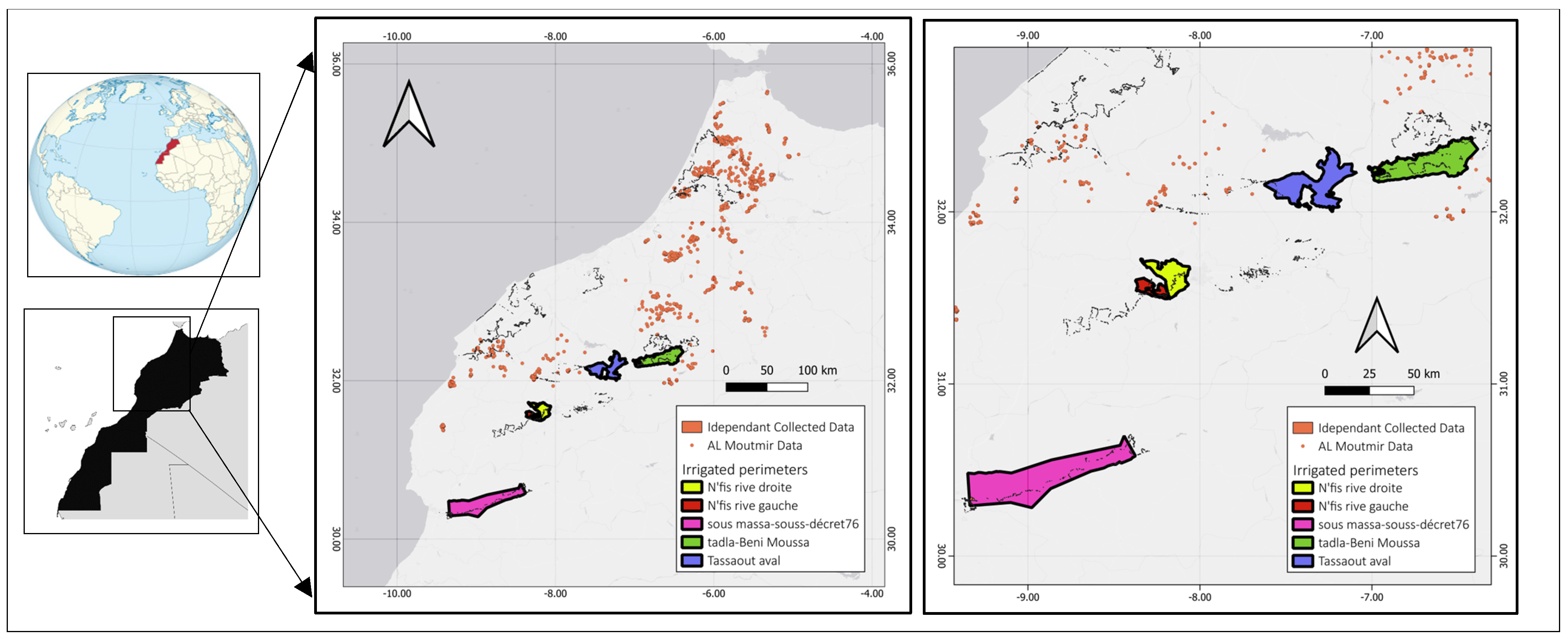
This study was conducted at two complementary spatial scales: a national calibration scale and a local application scale (Figure 1). At the national scale, field data were collected across Morocco’s major agricultural zones, covering the diversity of cropping systems, climatic conditions, and farming practices that characterize Moroccan agriculture. These data span a wide range of environments, from humid coastal lowlands to semi-arid continental plains, ensuring that the trained model captures the full spectral and phenological variability of the target classes.

At the local application scale, the classification framework was deployed over five strategic irrigated perimeters: (i) Tadla-Beni Moussa, (ii) Tassaout Amont, (iii) Tassaout Aval, (iv) Souss-Massa Decret 76, and (v) Nfis Rive Droite (Figure 1). These perimeters were selected for three primary reasons: (1) they represent Morocco’s most productive irrigated areas, contributing significantly to national cereal and tree-crop production; (2) they exhibit diverse cropping systems (cereals, citrus, olives, vegetables) and irrigation practices, providing a rigorous test for model transferability; and (3) official agricultural statistics are available for these perimeters, enabling direct validation of classification-derived crop areas against independent reference data. Morocco faces acute water scarcity and agricultural vulnerability to climate variability, with drought events increasing in frequency and severity over the past decade. The five strategic irrigation zones selected for this study represent critical agricultural production regions. Each zone exhibits distinct characteristics. The Moroccan government’s ‘Plan Maroc Vert’ and subsequent ‘Génération Green 2020–2030’ strategies require operational crop monitoring systems to support water allocation decisions and agricultural subsidies, yet current methods rely on costly annual field campaigns. This urgency, coupled with the region’s high inter-annual climate variability, makes Morocco an ideal testbed for stability-driven crop mapping approaches.

The study period spans six growing seasons (2018, 2019, 2020, 2023, 2024 and 2025), capturing the cumulative impact of multi-year drought and climate variability on crop dynamics and land-use changes, a critical factor for operational monitoring under changing environmental conditions. Agriculture remains a socioeconomic pillar in Morocco, yet operational crop maps are often outdated or coarse in resolution [28]. The agricultural years 2021 and 2022 were excluded due to a combination of an extreme drought that caused widespread crop failure and COVID-19-related travel restrictions that prevented field data collection. The combination of broad national coverage for model training and targeted application on irrigated perimeters for validation provides an ideal framework for assessing the scalability and robustness of satellite-based annual crop inventories in support of national food-security strategies.

2.2. Field Data Collection

The reference dataset used in this study was compiled from two complementary sources: (1) field surveys conducted by the Al Moutmir initiative [21] across multiple agricultural seasons (from 2018 to 2020), and (2) an independent dataset collected through systematic ground campaigns focusing on perennial crops and non-cereal land cover between 2023 and 2025.

The Al Moutmir data (n = 9582 samples) were collected during key phenological stages (sowing, growth, maturation, and post-harvest) and initially covered three dominant cereal crops: Soft Wheat, Durum Wheat, and Barley. To extend the classification framework to a more representative land cover system, these data were complemented with samples encompassing tree crops (olive, citrus, almond, and other perennial crops) and other cover types (bare soil, vegetables, and weeds), reclassified under the aggregated classes “Trees” and “Other Crops.” All samples were collected as georeferenced points or polygons using GPS, with careful attention to spatial and temporal consistency. Parcel boundaries were harmonized, and sample years were aligned based on the growing campaign (September–August). Specific product version numbers were not recorded, but the Google Earth Engine collections COPERNICUS/S2_SR_HARMONIZED and COPERNICUS/S1_GRD were used.

After spatial and temporal harmonization, the raw dataset comprised 9582 labeled samples across five classes: Soft Wheat, Durum Wheat, Barley, Trees, and Other Crops. To address the severe class imbalance (Soft Wheat dominant, approximately 67% of the raw samples), a stratified undersampling procedure was applied, capping each class at 1200 samples. This ensured equitable representation and prevented model bias toward the majority class. The final balanced dataset contained 4726 samples, split into training (80%) and test (20%) while preserving class proportions (

Table 1. Distribution of samples per class in the balanced dataset (4726 samples) after stratified undersampling.

Crop Class	Training Set	Test Set
Soft Wheat	865 (79.4%)	225 (20.6%)
Durum Wheat	637 (80.1%)	158 (19.9%)
Barley	605 (79.7%)	154 (20.3%)
Trees	716 (80.0%)	179 (20.0%)
Other Crops	950 (80.0%)	237 (20.0%)
Total	3773 (80%)	953 (20%)

). Missing values (<2% of monthly composites) were imputed using class-wise medians.

For the feature importance and stability analysis, we required a complete time series with no missing monthly composites. After removing samples with any missing months, 4753 samples remained.

Table 2. Raw samples per year and class (before filtering).

Year	Barley	Durum Wheat	Other Crops	Soft Wheat	Trees	Total
2018	162	125	6	104	0	397
2019	167	361	0	221	0	749
2020	430	309	0	765	0	1504
2023	0	0	84	0	158	242
2024	0	0	1097	0	737	1834
2025	0	0	12	0	15	27
Total	759	795	1199	1090	910	4753

shows the distribution of these 4753 samples by year and class. Note that the 2023–2025 campaigns contained only tree and other-crop samples because cereal field surveys were not conducted in those years due to drought and logistical constraints. No further filtering was applied after this step.

This explains the difference in sample sizes between the stability analysis (4753 samples) and the classification assessment (4726 samples). The 27 samples from the 2025 campaign lacked complete spatial coordinates and were therefore excluded from the classification dataset (

Table 3. Per-year pixel statistics for the stability analysis dataset (4726 samples). Each pixel corresponds to 10 m × 10 m (0.01 ha).

Year	Field Samples	Unique Pixels	Mean Samples/Pixel	Total Area (ha)
2018	397	185	2.15	1.85
2019	749	734	1.02	7.34
2020	1504	1407	1.07	14.07
2023	242	242	1.00	2.42
2024	1834	1834	1.00	18.34
Total	4726	4402	1.07 (mean)	44.02

).

Each field sample corresponds to a single Sentinel-2 pixel (10 m × 10 m = 0.01 ha). Because multiple samples from the same field (different years or different points within the same field) can fall on the same pixel, we deduplicated pixel coordinates for spatial analysis. As shown in Table 3, the overall mean number of samples per unique pixel was 1.07, with 2018 being the only year with notable pixel reuse (2.15 samples per pixel). This low overlap indicates that spatial dependence is limited. We acknowledge that spatial autocorrelation could influence accuracy estimates; however, the low samples-per-pixel ratio suggests that any such bias is likely minimal. Future work will incorporate explicit spatial blocking cross-validation to formally assess this.

2.3. Methodology

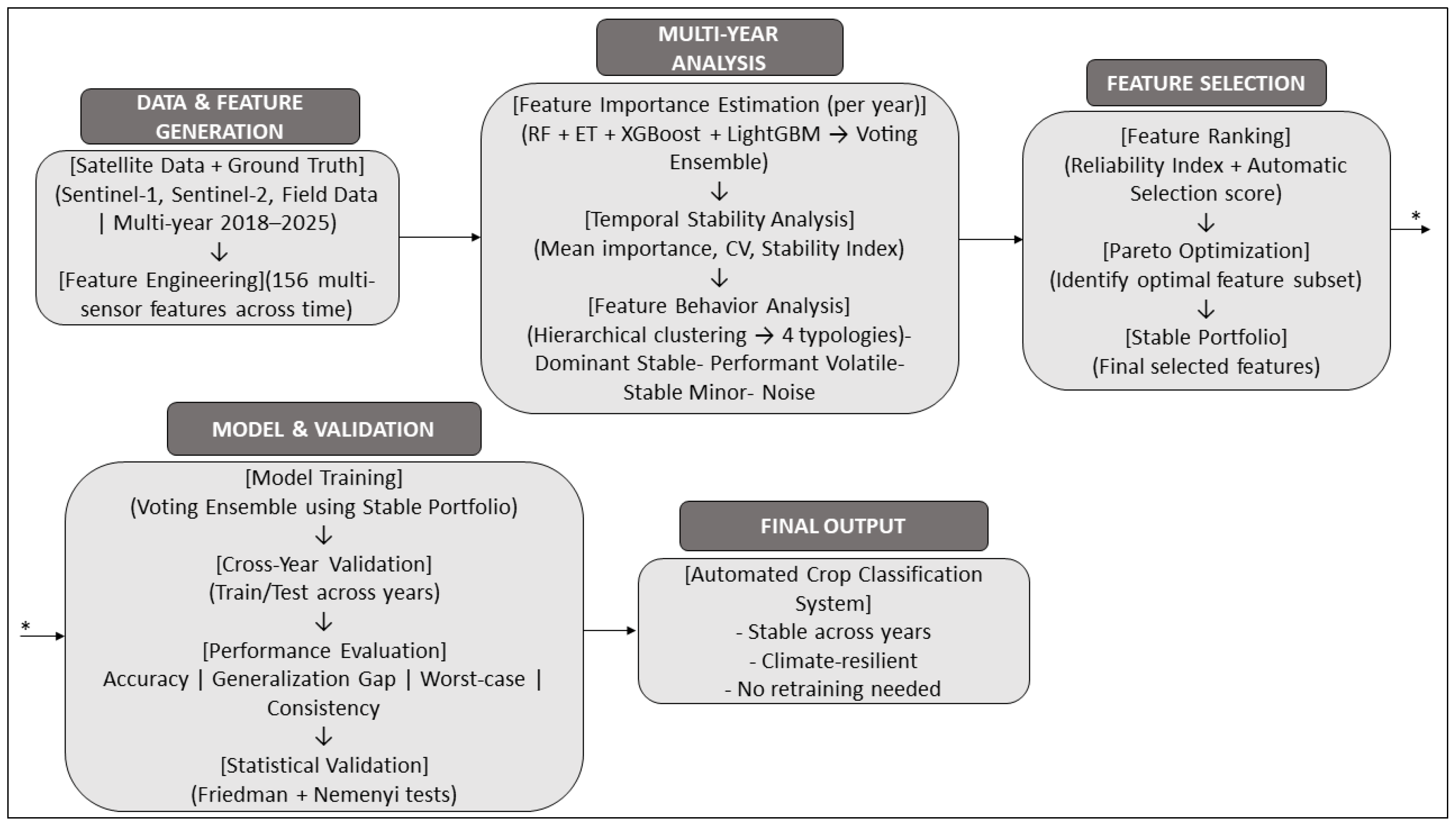
To evaluate the temporal stability of satellite-derived features for automated crop mapping, we developed a systematic framework combining multi-sensor feature engineering, Voting Ensemble consensus importance, statistical stability metrics, clustering analysis, and rigorous cross-year validation. The core objective is to understand how the importance of individual features fluctuates across years and to translate this understanding into a Stable Portfolio capable of robust year-to-year generalization with reduced need for annual retuning. This hybrid approach first uses Voting Ensemble consensus to derive stable importance metrics across multiple algorithms, then identifies a temporally robust feature portfolio, which is subsequently validated using high-performance classifiers for operational deployment [13,21]. The complete methodological workflow is illustrated in Figure 2.

2.3.1. Satellite Data Sources and Preprocessing

Multi-temporal optical and radar features were generated from Sentinel-2 and Sentinel-1 imagery to construct a phenology-aware, multi-sensor feature set covering six agricultural years (2018, 2019, 2020, 2023, 2024 and 2025) in Morocco [22]. All preprocessing and feature extraction were conducted using Google Earth Engine (GEE) Python 3.10 API within a Google Colab environment, enabling automated and reproducible multi-sensor data processing workflows over the defined study area, following established protocols for multi-sensor data fusion in agricultural applications. Sentinel-2 Level-2A surface reflectance data (bands B2, B3, B4, B8, B11, and B12) were filtered for cloud contamination. Images with <20% cloud cover over each irrigation zone were retained. This threshold was determined by sensitivity analysis showing that >20% cloud cover led to data gaps exceeding 35 days in more than 10% of pixels. Cloud detection at the pixel level: The Scene Classification Layer (SCL) was used to identify pixels with cloud, cirrus, or shadow status. Only pixels classified as ‘clear’ (SCL = 4), ‘vegetation’ (SCL = 5), ‘bare soil’ (SCL = 6), or ‘water’ (SCL = 7) were retained. Additionally, the QA60 band was used to mask clouds with bitwise And (1 << 10) and bitwise And (1 << 11) following standard practices. Monthly composite generation: For each month and each pixel, we computed the median of all clear observations within that month. No temporal interpolation was applied. If a month had fewer than three clear observations, the pixel was flagged as missing for that month. This approach preserves the original phenological signal without introducing interpolation artifacts. The percentage of missing monthly composites across all pixels was 2.3% for the full dataset. Rationale for median composites: The median is robust to outliers (e.g., undetected thin clouds) and does not assume any parametric form of the time series, unlike interpolation methods. This is particularly important for operational systems where cloud cover patterns are unpredictable.

The agricultural year was segmented into 12 monthly composites. For phenological interpretation, these months were grouped into four stages (three months each): Sowing/Emergence (September–November of the previous year), Vegetative Growth (December–February), Maturation (March–May), and Harvest/Post-harvest (June–August). Monthly composites were generated to minimize atmospheric and phenological noise while preserving sufficient temporal resolution to track crop development stages. From these composites, a comprehensive set of nine spectral indices was computed to capture complementary biophysical properties relevant to crop monitoring in semi-arid environments.

Table 4. Vegetation indices derived from Sentinel-2 imagery and their biophysical interpretations.

Index	Equation	Biophysical Significance	References
NDVI	${\displaystyle \frac{B_8-B_4}{B_8+B_4}}$	Vegetation vigor, green biomass	[30]
EVI	$2.5\times {\displaystyle \frac{B_8-B_4}{B_8+6\times B_4-7.5\times B_2+1}}$	Canopy structure, reduces atmospheric effects
GNDVI	${\displaystyle \frac{B_8-B_3}{B_8+B_3}}$	Green Normalized Difference Vegetation Index—sensitive to chlorophyll, suitable for high biomass
SAVI	${\displaystyle \frac{B_8-B_4}{B_8+B_4+0.5}} 1.5$	Soil-Adjusted Vegetation Index—minimizes soil brightness effects
BSI	${\displaystyle \frac{{(B}_{11}+B_4)-{(B}_8+B_2)}{{(B}_{11}+B_4)+{(B}_8+B_2)}}$	Bare Soil Index—detects bare soil and exposed surfaces	[31]
NDMI	${\displaystyle \frac{B_8-B_{11}}{B_8+B_{11}}}$	Canopy water content, moisture stress	[32]
NDBI	${\displaystyle \frac{B_{11}-B_8}{B_{11}+B_8}}$	Bare soil detection
NDRE	${\displaystyle \frac{B_8-B_5}{B_8+B_5}}$	Normalized Difference Red Edge Index—sensitive to chlorophyll content in dense canopies	[33]
GCVI	$\left({\displaystyle \frac{B_8}{B_3}}\right)-1$	Chlorophyll content, senescence detection	[34]

presents the complete list of indices, their formulations, and their biophysical significance. Each index was derived for all 12 months and appended with the month name (e.g., NDVI_Jan, EVI_Feb, SAVI_Mar), resulting in 108 optical feature time series (9 indices × 12 months). The raw spectral bands were not included in the stability analysis to focus on interpretable biophysical indices. For radar, four metrics (VV, VH, VH/VV ratio, RVI) were computed for each month, contributing 48 radar features (4 metrics × 12 months). The complete multi-sensor feature space thus comprised 156 features (108 optical + 48 radar). Capturing phenological shifts through harmonic modeling of time series has been shown to improve change detection robustness compared to fixed seasonal adjustments [29].

Dual-polarized Sentinel-1 Ground Range Detected (GRD) data (VV and VH) were retrieved in Interferometric Wide (IW) mode and temporally filtered to match the same monthly intervals. Median composites were computed for each month to reduce speckle noise and ensure radiometric consistency, following best practices for SAR time-series analysis in agricultural monitoring. In addition to raw backscatter (VV and VH), two derived radar indices were computed: the cross-polarization ratio (VH/VV) and the Radar Vegetation Index (RVI). The VH/VV ratio enhances sensitivity to crop structural changes and volumetric biomass while reducing the influence of soil moisture and surface roughness [35]. The RVI provides a measure of vegetation structure complexity, with higher values indicating denser, more complex canopies typical of perennial woody crops [36]. Including these derived indices is particularly valuable for discriminating perennial woody crops (e.g., olive, citrus) from annual cereals, as they capture the volume scattering signature of tree canopies. Radar features contributed 48 features (VV, VH, VH/VV, RVI × 12 months).

Feature stacking and masking: For each year, all optical bands, vegetation indices, and radar backscatter coefficients were concatenated into a single multi-sensor feature stack.

Table 5. Composition of the multi-sensor feature space (156 features total).

Feature Category	Number of Features	Description
Vegetation Indices (S2)	108	9 indices (NDVI, NDRE, NDMI, EVI, SAVI, GNDVI, GCVI, NDBI, BSI) × 12 months
Radar Backscatter (S1)	48	4 metrics (VV, VH, VH/VV, RVI) × 12 months
Total	156	Complete multi-sensor stack (108 + 48 = 156)

summarizes the complete feature space composition.

A crop mask was generated using the NDVI composite from the growth stage, applying a threshold of NDVI > 0.3 to exclude non-vegetated or fallow areas. The resulting masked stack ensured consistent phenological alignment across years, enabling robust feature stability analysis and cross-season model validation.

2.3.2. Harmonization of Sentinel-1 and Sentinel-2 Spatial Resolution

To ensure consistent spatial resolution across all input features from the two sensors, a standardized harmonization workflow was applied. For Sentinel-2, bands with native 20 m spatial resolution (B5, B6, B7, B8a, B11, B12) were resampled to 10 m using bilinear interpolation, while bands with native 10 m resolution (B2, B3, B4, B8) were used as is. The coastal aerosol band (B1, 60 m) and the water vapor band (B9, 60 m) were excluded from the analysis as they do not contribute to vegetation or crop discrimination.

For Sentinel-1, the Ground Range Detected (GRD) product in Interferometric Wide (IW) mode with dual polarization (VV + VH) was processed through a series of standard steps. Thermal noise removal was applied automatically by the Google Earth Engine default implementation. Radiometric calibration was then performed to convert digital numbers to backscatter coefficient σ⁰ in a linear scale. Speckle noise was reduced using a refined Lee filter with a 5 × 5 window, followed by terrain correction using the SRTM 30 m digital elevation model to compensate for topographic effects. The resulting backscatter images were subsequently resampled to a 10 m grid to match the spatial resolution of Sentinel-2. Finally, the linear backscatter values were converted to decibels using the transformations VH_dB = 10·log₁₀(VH) and VV_dB = 10·log₁₀(VV), which is standard practice for radar data visualization and analysis.

Co-registration between the two sensor products was verified by manually identifying control points, such as road intersections and field corners, for each irrigation zone. The root mean square error (RMSE) of the geometric alignment was consistently below 0.5 pixels, confirming that no further geolocation correction was necessary.

2.3.3. Multi-Model Importance Estimation via Voting Ensemble Consensus

A critical innovation of this study is the use of Voting Ensemble consensus rather than a single classifier for feature importance estimation. This approach leverages diversity across multiple algorithms to filter out model-specific noise and reveal the underlying phenological signal that multiple models agree upon. This is a property that is essential for automated systems.

We selected tree-based ensemble models (Random Forest, Extra Trees, XGBoost, LightGBM) for three reasons. First, they provide native feature importance measures without requiring additional permutation calculations, which is essential for our stability-driven feature selection framework. Second, they handle mixed data types (optical indices and radar backscatter) without normalization or special preprocessing. Third, they are computationally efficient for high-dimensional time series (156 monthly features × 4726 samples × 100 trees ≈ 15 min training), which is critical for operational deployment. While we acknowledge that including fundamentally different models (e.g., SVM or neural networks) could potentially increase ensemble diversity, this would come at the cost of significantly higher computational complexity and loss of native feature importance estimation. As our primary objective is operational automation with minimal expert intervention, we opted for the tree-only ensemble. This choice is consistent with recent large-scale crop mapping studies that favor tree-based ensembles for their balance of accuracy, interpretability, and efficiency [37].

For each year independently (2018, 2019, 2020, 2023, 2024, and 2025), we trained a suite of classifiers on the annual ground truth data comprising the five crop classes.

Table 6. Classifier suite for Voting Ensemble consensus importance estimation.

Classifier	Key Parameters	Importance Extraction Method
Random Forest (RF)	n_estimators = 100, criterion = ‘gini’	Mean Decrease in Impurity (Gini)
Extra Trees (ET)	n_estimators = 100, criterion = ‘gini’	Mean Decrease in Impurity (Gini)
XGBoost	n_estimators = 100, learning_rate = 0.1	Gain-based importance
LightGBM	n_estimators = 100, learning_rate = 0.1	Split-based importance

presents the suite of classifiers and their key parameters.

Feature importance was extracted from each model using their native importance metrics, following established methodologies for multi-model importance assessment. The Voting Ensemble consensus importance for feature i in year y was then defined as the median of the four model-specific importance values:

Let $f_i^{y,RF},f_i^{y,ET},f_i^{y,XGB},f_i^{y,LGB}$ be the importance of feature $i$ (where $i$ ranges over the 156 monthly features) in agricultural year $y$ (where $y$ ∈ {2018, 2019, 2020, 2023, 2024, 2025} from) Random Forest, Extra Trees, XGBoost, and LightGBM, respectively. The Voting Ensemble consensus importance is as follows:

$$f_i^y=median\left(f_i^{y,RF},f_i^{y,ET},f_i^{y,XGB},f_i^{y,LGB}\right)$$

The median was chosen over the mean to ensure robustness against outlier importance estimates from any single algorithm, a strategy recommended for ensemble-based feature selection. This produced a temporal importance profile vector for each feature across the six agricultural campaigns:

$$\overrightarrow{f_i}=\left[f_i^{2018},f_i^{2019},f_i^{2020},f_i^{2023},f_i^{2024},f_i^{2025}\right]$$

All subsequent stability analyses are based on these multi-annual consensus vectors, ensuring that our findings reflect multi-model agreement across diverse climatic conditions rather than single-algorithm or single-year bias. Future work will explore deep learning architectures to automatically learn stable feature representations directly from raw time series, potentially capturing non-linear phenological patterns beyond hand-crafted indices.

2.3.4. Hyperparameter Configuration

The hyperparameters of the four base classifiers were determined through iterative experimentation using 5-fold cross-validation on the 2018–2020 training data (3000 samples). For Random Forest and Extra Trees, we tested n_estimators in {100, 200, 250, 300}, max_depth in {10, 15, 20, None}, min_samples_split in {2, 5, 8, 10}, and selected the values that maximized validation F1-score while minimizing the training-validation gap. The final configuration was: n_estimators = 250, max_depth = 15, min_samples_split = 8, min_samples_leaf = 4. For XGBoost and LightGBM, we explored n_estimators up to 700, learning_rate in {0.01, 0.03, 0.05, 0.1}, reg_alpha and reg_lambda in {0, 1, 2, 5}, and selected n_estimators = 500, learning_rate = 0.03, max_depth = 6, reg_alpha = 2.0, reg_lambda = 2.0 for XGBoost, and num_leaves = 50, min_child_samples = 10 for LightGBM. Models converged stably, with out-of-bag error (RF, ET) and validation loss (XGB, LGB) changing by less than 0.1% over the last 50 training rounds. Using default parameters reduced test accuracy by approximately 2 percentage points, confirming the benefit of case-specific tuning.

2.3.5. Stability and Volatile Metrics

To assess how consistently each feature contributed to classification across the six agricultural years, we computed multiple statistical metrics from the consensus importance vectors (

Table 7. Definitions of stability and volatility metrics.

Metric	Formula	Interpretation
Mean Importance (${\mu }_i)$	${\displaystyle \frac{1}{n}}{\sum }_y{f}_i^y$	Average contribution across years
Standard Deviation $({\mathsf{\sigma }}_i$)	$\sqrt{{\displaystyle \frac{1}{n}}}{\sum }_y{(f_i^y-{\mu }_i)}^2$	Absolute variability
Coefficient of Variation (CV)	${\displaystyle \frac{{\mathsf{\sigma }}_i}{{\mu }_i}}$	Relative volatility (scale-invariant)
Stability Index ${(S}_i$)	${\displaystyle \frac{1}{({CV}_i+\mathsf{ϵ})}}$	Inverse volatility; higher = more stable
Max/Min Ratio $R_i$	$\max \left(f_i^y\right)/\mathrm{m}\mathrm{i}\mathrm{n}\left(f_i^y\right)+\mathsf{ϵ}$	Extreme fluctuation range

).

For a given feature $i$ let ${\mu }_i$ be its mean importance across the six agricultural years (2018, 2019, 2020, 2023, 2024 and 2025), and ${\mathsf{\sigma }}_i$ its standard deviation.

Where n = 6 (number of years) and ϵ = 10⁻⁸ ensures numerical stability. Features with ${CV}_i>0.5$ were considered volatile, while those with high $S_i$ were considered stable, following thresholds established in recent feature stability literature [38].

We assign the same stability value to all monthly composites of a given spectral index, based on the observation that the relative stability of different indices is consistent across months. A preliminary inspection of month-wise stability suggested strong consistency across months; therefore, using a single annual stability value per index simplifies the framework without substantial loss of information.

Foundational work on time series stability has established the coefficient of variation as a key metric for quantifying inter-annual variability [39]. Methods for detecting abrupt and gradual changes in vegetation time series, such as BFAST (Breaks For Additive Seasonal and Trend), also rely on stability concepts to distinguish disturbances from seasonal variability [40]. More recent studies have confirmed the utility of tree-based ensembles for crop classification [41] and the feasibility of large-scale Sentinel-2 mapping [42].

2.3.6. Advanced Selection Metrics: RI and AuSS

Moving beyond descriptive statistics, we introduced two novel composite indices designed specifically for operational feature selection, balancing predictive power with temporal robustness.

Table 8. Novel composite indices for operational feature selection.

Metric	Formula	Operational Significance
Reliability Index (RI)	${RI}_I={\mathsf{\mu }}_i/({CV}_i+ϵ)$	Direct importance-stability trade-off; identifies consistent high-performers
Automatic Selection Score (AuSS)	${AuSS}_i={\mu }_i\times \mathrm{l}\mathrm{n}(1+S_i)$	Balances importance with logarithmic stability penalty; designed for automation ranking

presents these metrics and their operational significance.

The Reliability Index (RI) directly quantifies the importance-stability trade-off by rewarding high mean importance while penalizing high volatility. A high RI identifies features that are consistently valuable across years, potential “pillars” for an automated system.

The Automatic Selection Score (AuSS) balances absolute importance with a logarithmic scaling of stability, preventing the selection of extremely stable but non-informative features. The logarithmic transformation ensures that diminishing returns in stability do not disproportionately penalize highly important but moderately stable features, making it particularly suitable for automated pipeline design. The logarithmic transformation prevents extremely stable features from dominating the ranking, ensuring that features with moderate stability but high importance are not penalized excessively.

2.3.7. Design Rationale and Sensitivity of Stability Metrics

The choice of the Reliability Index ${RI}_I={\mathsf{\mu }}_i/({CV}_i+ϵ)$ was guided by three requirements: (1) higher mean importance μ should increase the score; (2) higher inter-annual variability (measured by CV) should decrease the score; (3) the metric should be dimensionless to allow comparison between optical indices (unitless) and radar backscatter (decibels). The small constant ϵ = 10⁻⁸ prevents division by zero when ${\mu }_i=0$.

The Automatic Selection Score ${AuSS}_i={\mu }_i\times \ln \left(1+S_i\right)$ uses the Stability Index ${(S}_i$). The natural logarithm applies a diminishing returns penalty: as stability increases, the marginal gain in AuSS decreases. This avoids over-weighting features with extremely high stability while still penalizing low stability. The addition of 1 inside the logarithm ensures ${AuSS}_i=0$ when $S_i=0$ (i.e., when ${CV}_i\to \mathrm{\infty }).$

Sensitivity analysis: To assess the impact of the CV threshold on feature selection, we varied the threshold used to identify “stable” features from 0.20 to 0.40 (the default 0.25 lies within this range). The number of stable monthly features changed predictably, but the top-10 features ranked by AuSS remained consistent (Jaccard similarity > 0.85). The Pareto-optimized portfolio of six indices (VH, VV, NDVI, NDRE, GCVI, RVI) did not change across thresholds. This confirms that our metric choices and thresholds are robust for operational use.

2.3.8. Hierarchical Clustering and Behavioral Typology

To uncover latent patterns and group features with similar temporal dynamics, we applied hierarchical clustering to the normalized consensus importance vectors. Features were normalized to a unit range to ensure temporal pattern, rather than magnitude, drove clustering:

$$\widetilde{f_i^y}={\displaystyle \frac{f_i^y-\mathrm{m}\mathrm{i}\mathrm{n}\left(f_i\right)}{\max \left(f_i\right)-\min \left(f_i\right)+ϵ}}$$

Clustering was performed using Euclidean distance with Ward’s linkage method, which minimizes within-cluster variance and produces compact, interpretable clusters. Analysis of these clusters in the Mean Importance vs. Stability space revealed a coherent four-quadrant behavioral typology, summarized in

Table 9. Four-quadrant behavioral typology of features.

Quadrant	Importance	Stability	Operational Role
Dominant Stable	High	High	Portfolio Ideal—Core automation features
Performant Volatile	High	Low	Climatically sensitive—Use conditionally
Stable Minor	Low	High	Structural anchors—Baseline consistency
Noise/Unstable	Low	Low	Candidates for pruning

.

This typology provides a strategic framework for feature management in operational systems, enabling informed decisions about which features to retain, which to monitor conditionally, and which to discard.

2.3.9. Feature Portfolio Construction and Subset Definitions

Based on the above analyses, we constructed specific feature subsets to evaluate different selection strategies.

Table 10. Feature subsets for comparative evaluation.

Subset Name	Selection Criteria	Number of Features	Purpose
Full Feature Set	All available features	156	Baseline (conventional approach)
Stable Portfolio	Pareto-optimized by AuSS	72	Core output—automated system
Stable Set	Top-ranked by Si	15	Benchmark: pure stability
Volatile Set	Top-ranked by σi	15	Benchmark: pure importance (unstable)
Top-RI Set	Top-ranked by RI	15	Benchmark: importance-stability balance
Top-ASS Set	Top-ranked by ASS	15	Benchmark: automation ranking

presents the feature subsets used in this study.

The Stable Portfolio was identified via Pareto analysis of features ranked by the Automatic Selection Score (AuSS). The Pareto pivot point was determined where cumulative predictive importance reached a plateau (77.9% at n = 72 features), capturing the majority of robust signal while filtering out inter-annual noise.

2.3.10. Cross-Year Evaluation Protocol

To ensure rigorous temporal generalization assessment, training and testing samples were strictly separated by agricultural year. No sample from a test year was used for model training. Spatial separation (by geographic location or individual field parcel) was not applied across different years because the same field parcel can contain different crops in different years; however, the same parcel never appears in both training and testing sets within a single year. The six available years (2018, 2019, 2020, 2023, 2024 and 2025) were combined into nine train-test configurations: (1) train on every single year and test on all other years (six configurations); (2) train on the three pre-gap years (2018–2020) and test on each post-gap year (2023, 2024, 2025 three configurations).

A rigorous temporal validation protocol was implemented to assess generalization performance, the true test of operational readiness. For each feature subset, models were trained on data from specific years and tested on independent years, resulting in multiple train-test combinations that reflect the temporal transfer challenge. The six available years (2018, 2019, 2020, 2023, 2024 and 2025) allow for comprehensive evaluation of model robustness across different climatic conditions.

Table 11. Performance metrics for cross-year validation.

Metric	Definition	Interpretation
Same-Year Accuracy	Average when train = test year	Upper bound performance
Cross-Year Accuracy	Average across different years	True operational performance
Generalization Gap	Same-Year—Cross-Year	Penalty for temporal transfer
Worst-Case Accuracy	Minimum across all test years	Risk assessment
Consistency	1-std (Accuracies)	Stability of performance

presents the performance metrics computed for each evaluation.

Final Ensemble Validation: Using the Stable Portfolio as the sole input feature space, we trained and validated the Voting Ensemble (combining RF, Extra Trees, XGBoost, and LightGBM) to represent the target operational system. The performance differences between feature subsets were subsequently assessed for statistical significance using paired t-tests and the non-parametric Friedman test with post hoc Nemenyi analysis (α = 0.05). Visualizations included grouped bar charts, radar plots, and boxplots for performance comparison (see Section 3).

3. Results

3.1. Phenological Patterns of Feature Stability

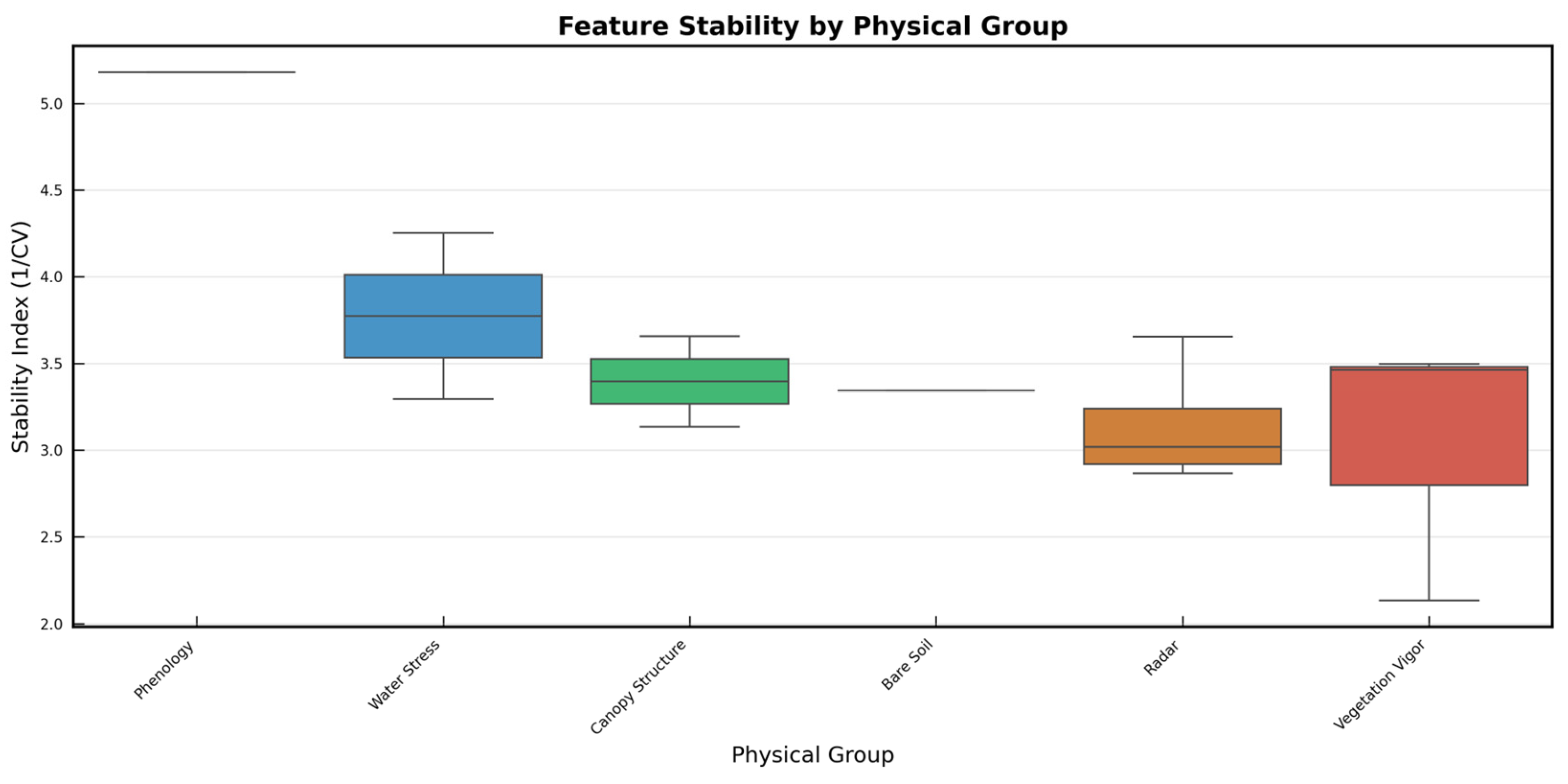
Stability, defined as the inverse of the coefficient of variation (1/CV), is computed at the feature level across years. As a result, all monthly instances of a given spectral index share the same stability value, since stability reflects inter-annual variability rather than intra-annual dynamics. Consequently, grouping by phenological stages (sowing, growth, maturation, harvest) yields identical stability distributions, while substantial differences emerge between indices. Figure 3 illustrates these differences through a boxplot grouping indices by their physical category. The Phenology group (NDRE) exhibits the highest stability, with a nearly degenerate distribution reflecting both its strong temporal consistency and the limited number of features in this category. Water Stress indices (NDMI, MSI) and Canopy Structure indices (EVI, SAVI) follow, showing relatively high and consistent stability. In contrast, Radar and Vegetation Vigor indices (NDVI, GNDVI, GCVI) display lower median stability and greater dispersion, with the latter showing the widest spread, indicating higher sensitivity to inter-annual climatic variability.

Table 12. Ranking of the 13 indices by the Reliability Index (RI).

Index	Stability (1/CV)	Sensor Family
NDRE	5.18	Optical
NDMI	4.25	Optical
SAVI	3.66	Optical
RVI	3.65	Radar
GCVI	3.50	Optical
NDVI	3.46	Optical
BSI	3.34	Optical
MSI	3.29	Optical
EVI	3.14	Optical
VH	3.10	Radar
Ratio	2.94	Radar
VV	2.87	Radar
GNDVI	2.13	Optical

further quantifies this hierarchy by ranking the 13 indices according to their stability. The red-edge index NDRE emerges as the most stable feature (5.179), followed by water stress indices NDMI (4.251) and MSI (3.294). At the lower end, vegetation vigor indices such as GNDVI (2.133) and NDVI (3.461) exhibit higher variability, reflecting their sensitivity to environmental fluctuations. Radar-based features (VH, VV, Ratio, RVI) occupy an intermediate range (2.866–3.654), supporting their role as relatively stable structural indicators across years.

3.2. The Fundamental Trade-Off: Importance vs. Stability

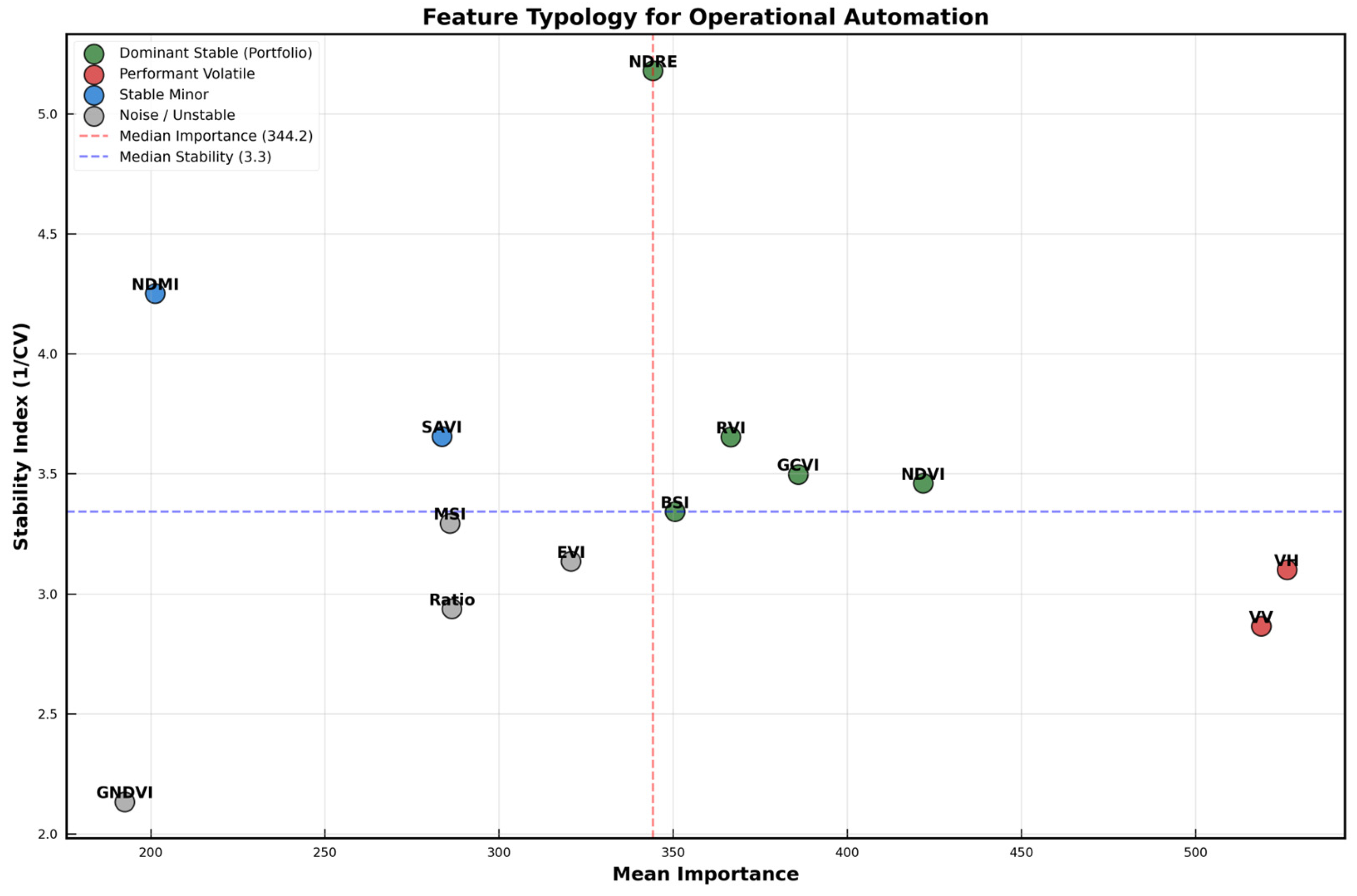
The relationship between predictive importance (mean importance across years) and temporal stability is illustrated in Figure 4. The scatter plot is divided by the median importance (344.25) and median stability (3.3423), defining four distinct behavioral quadrants:

• Dominant Stable (high importance, high stability): BSI, GCVI, NDRE, NDVI, RVI. These indices form the ideal core for an automated system, combining strong discriminative power with consistent inter-annual performance.
• Performant Volatile (high importance, low stability): VH, VV. They provide excellent predictive capability, but are highly sensitive to climatic variability, requiring conditional use.
• Stable Minor (low importance, high stability): NDMI, SAVI. They serve as structural anchors, offering reliable but modest contributions.
• Noise/Unstable (low importance, low stability): EVI, GNDVI, MSI, Ratio. These indices contribute little and vary unpredictably, making them clear candidates for pruning.

This four-quadrant typology, derived from Voting Ensemble consensus, provides a framework for feature selection: retain Dominant Stable indices as the foundational portfolio, employ Performant Volatile indices adaptively, keep Stable Minor indices as baseline anchors, and eliminate the Noise group to reduce overfitting and improve generalization.

3.3. Confusion Matrix of the Stable Portfolio

To complement the stability-driven analysis,

Table 13. Average confusion matrix (%) for the Stable Portfolio across test years.

True Class ↓/Predicted Class →	Soft Wheat	Durum Wheat	Barley	Trees	Other Crops
Soft Wheat	85.3	10.7	0.0	1.8	2.2
Durum Wheat	11.4	78.5	4.4	3.2	2.5
Barley	1.9	1.9	94.2	0.0	2.0
Trees	1.1	0.0	0.6	94.5	3.8
Other Crops	5.1	0.8	3.3	4.8	86.0

Note: The downward arrow (↓) denotes the true (reference) classes listed in the rows, whereas the rightward arrow (→) denotes the predicted classes listed in the columns.

presents the confusion matrix (row-wise normalized percentages) for the Stable Portfolio model, averaged over the three test years (2019, 2020, 2024). Values indicate the percentage of true class *c* (rows) predicted as each class (columns).

The most frequent misclassifications occur between Soft Wheat and Durum Wheat (≈11–14%), reflecting their spectral-phenological similarity. Tree crops are the best discriminated class (94.5% accuracy), while “Other Crops” (including vegetables, fallow, and weeds) show moderate confusion with cereal classes (≈9% total). A detailed multi-model classification benchmark, including per-class F1-scores, ROC curves, and year-wise confusion matrices, is provided in a companion study focusing on classifier optimization [36].

3.4. Top Stable Pillars for Operational Automation

To operationalize this trade-off, we ranked all features by the Reliability Index (RI), defined as the ratio of mean importance to the coefficient of variation, defined as follows:

$${RI}_i={\displaystyle \frac{{\mu }_i}{{CV}_I+\epsilon }}$$

This metric directly identifies features that balance predictive power with temporal consistency.

Table 14. Top 10 features by Reliability Index (RI).

Rank	Index	Mean Importance	RI	Sensor
1	NDRE	344.25	1782.93	Optical
2	VH	526.25	1631.65	Radar
3	VV	518.83	1486.70	Radar
4	NDVI	421.75	1459.51	Optical
5	GCVI	385.92	1349.95	Optical
6	RVI	366.50	1339.28	Radar
7	BSI	350.50	1171.46	Optical
8	SAVI	283.58	1036.78	Optical
9	EVI	320.67	1005.23	Optical
10	MSI	285.92	941.74	Optical

presents the top-ranked features according to RI. The red-edge index NDRE ranks first, confirming its strong combination of high importance and low variability. Radar features (VH, VV, RVI) also occupy prominent positions, highlighting their relatively consistent behavior across varying environmental conditions. Vegetation indices such as NDVI and GCVI appear among the top-ranked features, indicating that certain optical signals retain both discriminative power and acceptable temporal stability. These results suggest that early-stage spectral responses may be more robust than commonly assumed. Overall, the RI-based ranking confirms that combining importance and stability provides a more reliable basis for feature selection than considering either criterion independently.

3.5. Sensor Complementarity: Synergy of Optical and Radar

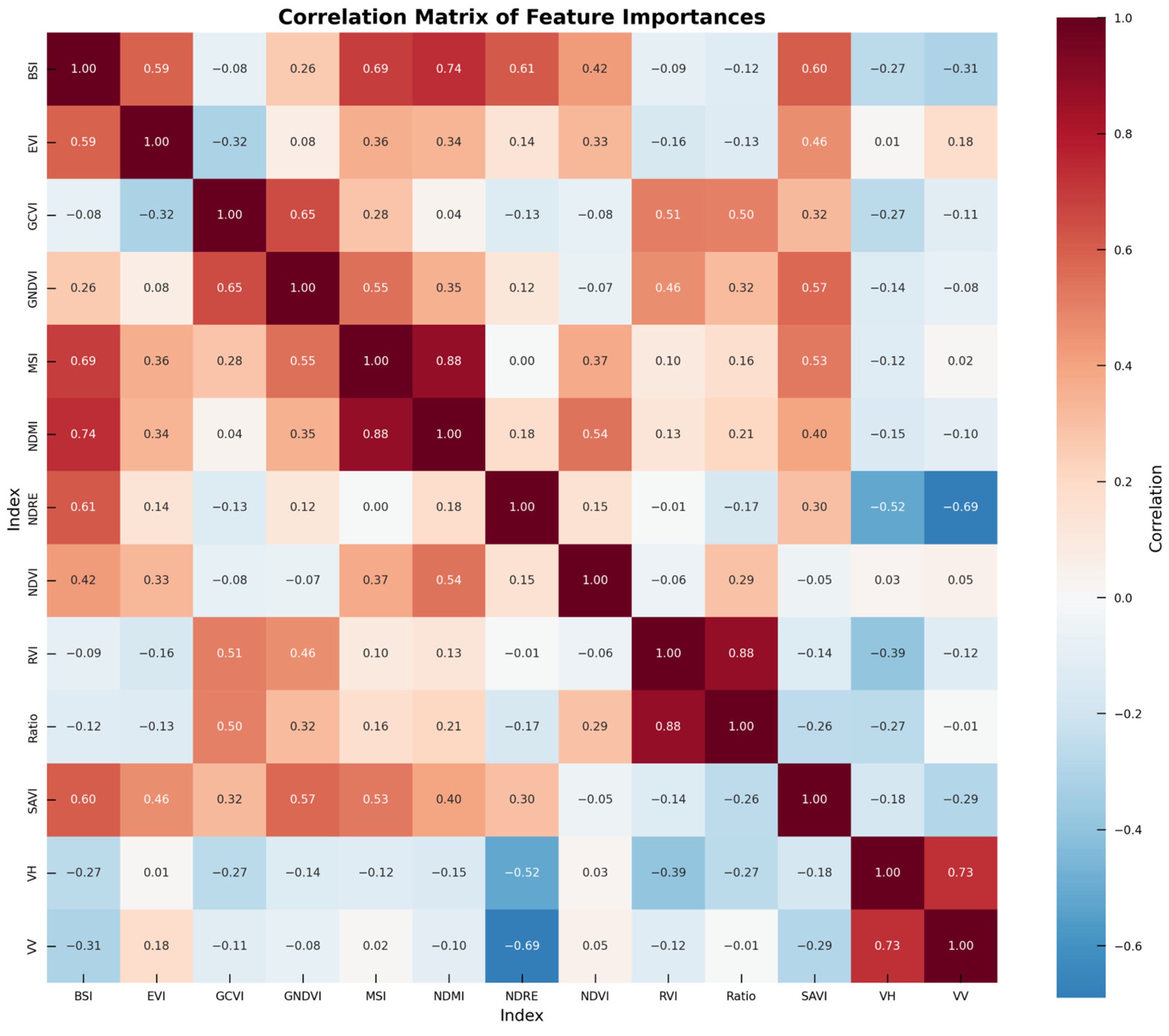
The correlation matrix of the 13 indices (Figure 5) reveals two distinct patterns. First, strong intra-family correlations indicate redundancy among features derived from similar physical processes. For example, MSI and NDMI exhibit a high correlation (r = 0.88), as do RVI and Ratio (r = 0.88), suggesting that one feature from each pair may be sufficient. Second, cross-correlations between radar and optical indices remain consistently low (|ρ| < 0.3), confirming that the two sensor families provide complementary information. Optical indices primarily capture biochemical properties such as chlorophyll content and leaf area index, whereas radar backscatter is sensitive to structural and dielectric properties of the canopy.

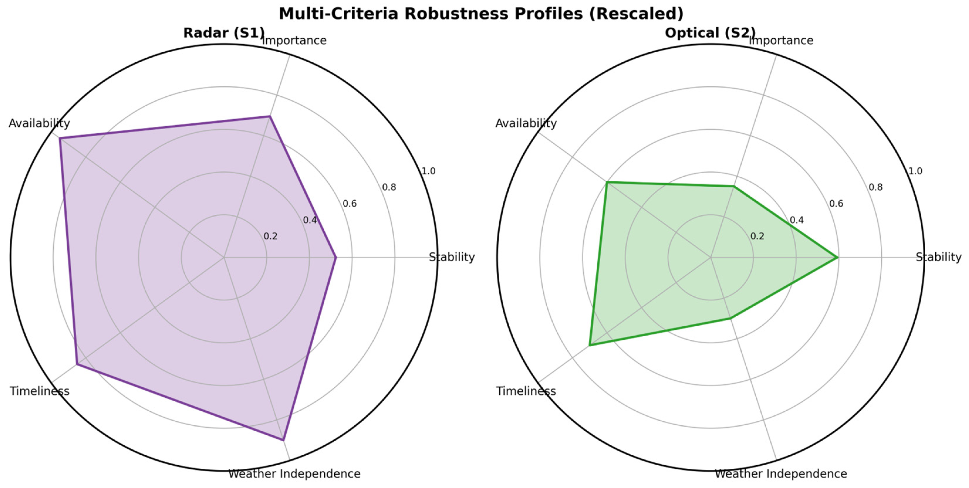
To further investigate sensor complementarity, a multi-criteria robustness comparison was performed using five criteria: Stability, Importance, Availability, Timeliness, and Weather Independence (Figure 6). Stability and Importance were obtained directly from the quantitative feature-analysis framework, where Stability corresponds to the mean Stability Index and Importance corresponds to the mean feature importance across years. The remaining criteria represent operational characteristics of the sensor families. Availability reflects the consistency of usable observations throughout the growing season, Timeliness reflects the ability to support early-season crop discrimination, and Weather Independence reflects resilience to cloud contamination and adverse atmospheric conditions. To facilitate comparison among heterogeneous criteria, all metrics were normalized to a common 0–1 scale. While Stability and Importance are derived from quantitative analysis, the operational criteria provide complementary contextual information intended to summarize the practical advantages and limitations of radar and optical observations in agricultural monitoring.

After normalization to a common scale, radar and optical sensor families exhibit distinct yet complementary robustness patterns. Radar features achieve higher scores for Availability, Timeliness, and Weather Independence, reflecting their capacity to provide consistent observations regardless of cloud cover and support crop monitoring from the earliest stages of the growing season. Optical features exhibit slightly higher Stability and contribute detailed spectral and phenological information that is particularly valuable during key crop development stages. These results suggest that neither sensor family alone fully captures the diversity of information required for robust crop classification. Instead, their integration provides a balanced framework in which radar data ensures operational continuity and resilience, while optical observations contribute complementary phenological and spectral detail under favorable acquisition conditions.

3.6. Temporal Trajectory of Predictive Information

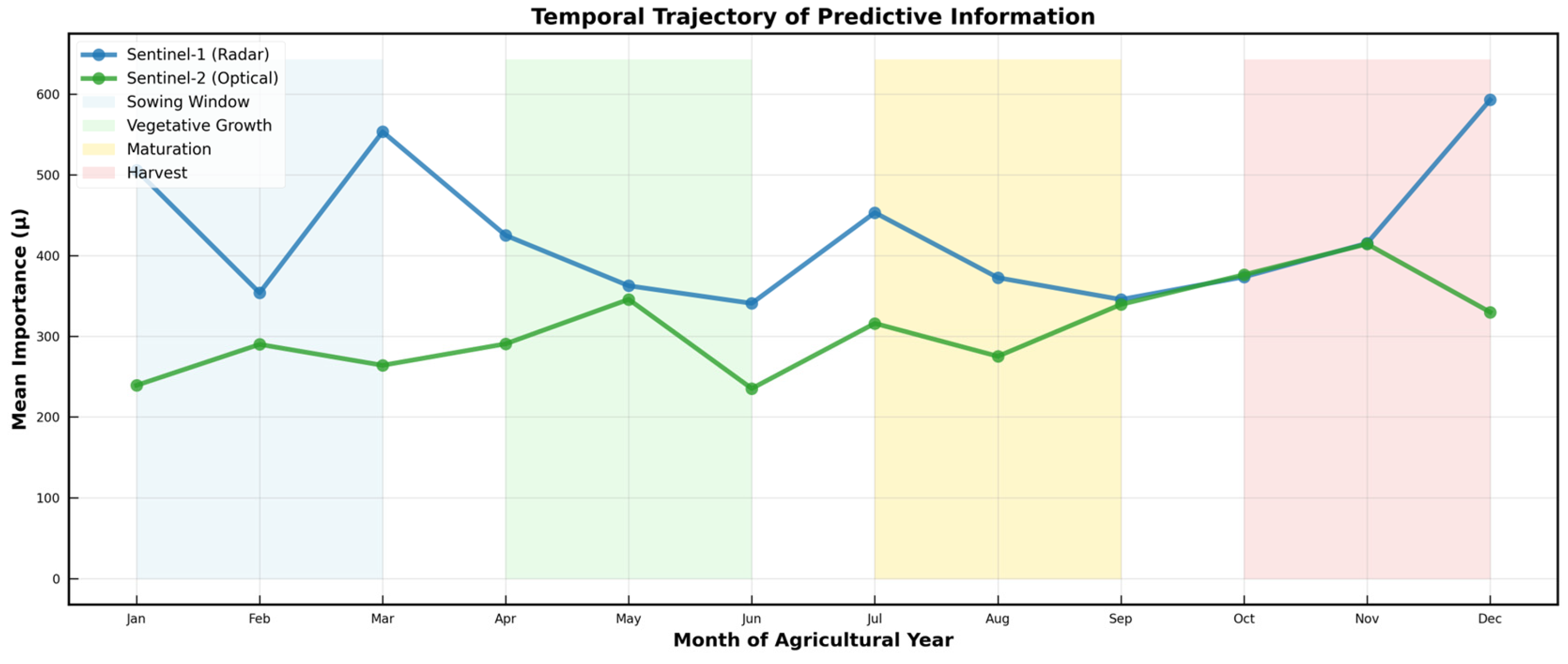
Feature importance is not static but varies throughout the agricultural season, reflecting changes in crop development and environmental conditions. To capture this dynamic behavior, Figure 7 presents the temporal evolution of mean consensus importance for radar and optical features, with shaded regions indicating inter-annual variability (±1 standard deviation).

Radar features exhibit consistently high importance across the entire season, with noticeable increases during key transition periods such as early growth, mid-season, and harvest. This suggests that radar provides a stable and continuous source of predictive information, largely independent of seasonal constraints. In contrast, optical features display a more variable trajectory, with importance increasing during periods of active vegetation development and declining during early and late stages of the season. This behavior reflects the sensitivity of optical signals to vegetation dynamics and their dependence on favorable acquisition conditions. These contrasting temporal patterns highlight the complementary roles of radar and optical data, with radar ensuring consistent baseline performance and optical features contributing enhanced discriminative power during specific phenological stages.

3.7. Pareto Optimization: Pruning Noise, Preserving Signal

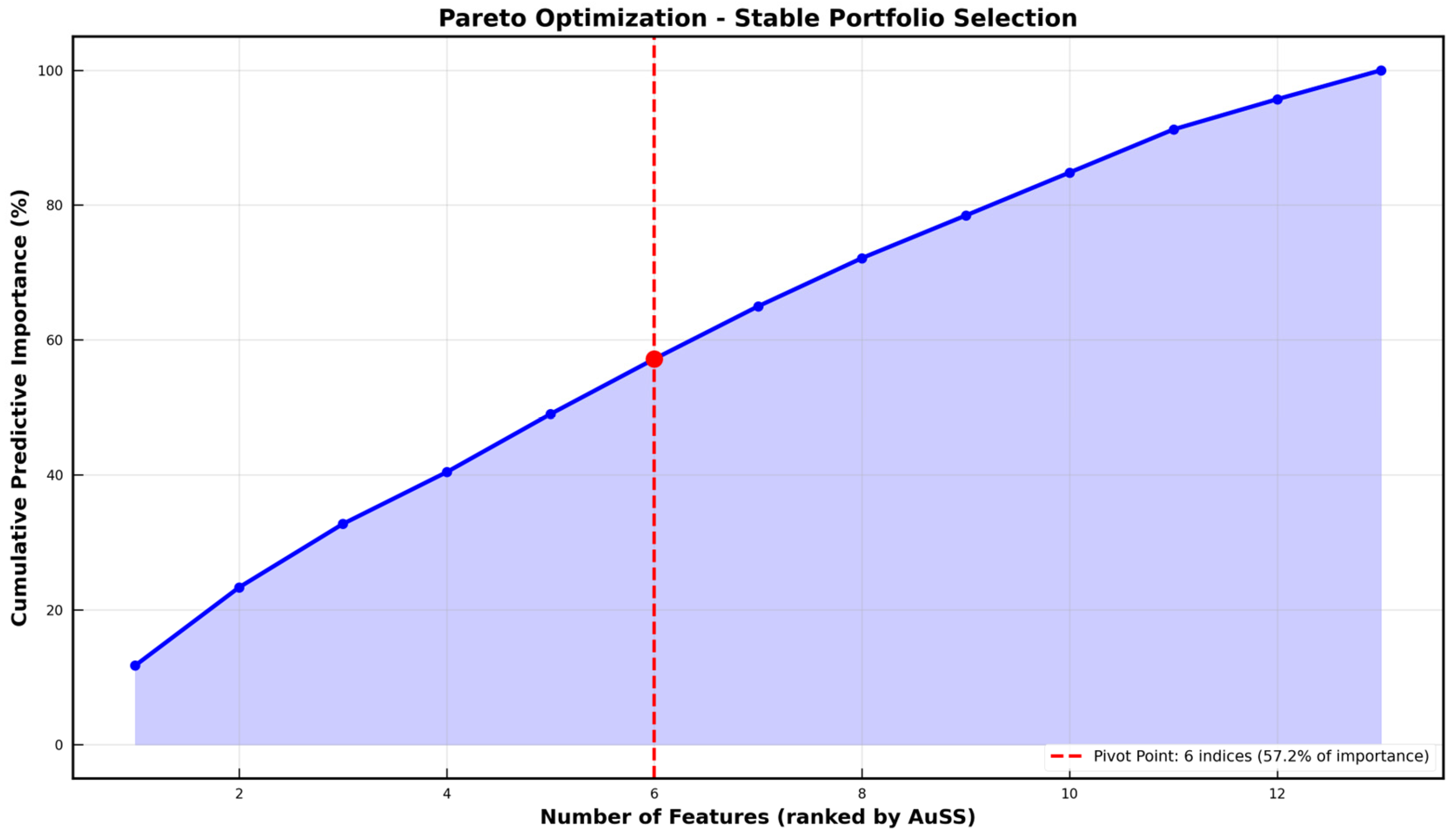
The consensus importance derived from the Voting Ensemble across six years enables the identification of diminishing returns in feature accumulation. To determine an optimal feature subset for automated classification, all 156 features were ranked according to their Automatic Selection Score (AuSS), and the cumulative proportion of total predictive importance was computed as a function of the number of selected features.

The resulting Pareto curve (Figure 8) reveals a clear diminishing return behavior, where the initial features contribute disproportionately to the overall predictive signal. A distinct inflection point is observed at approximately six features, which together account for about 57% of the cumulative importance. These six features correspond to spectral indices (VH, VV, NDVI, NDRE, GCVI, RVI). For each selected index, all 12 monthly composites (September to August) are retained, resulting in a Stable Portfolio of 72 monthly features (6 indices × 12 months). The cumulative importance percentage (57.2%) refers to the index-level importance—i.e., the sum of the importances of the 12 monthly composites for each index, normalized by the total importance of all 156 monthly features. Thus, the reduction in the number of monthly features is also 54% (from 156 to 72). Beyond this point, the marginal contribution of additional features decreases substantially, indicating increasing redundancy within the feature space. This suggests that a relatively small subset of features captures the majority of stable and informative signal, while the remaining features contribute limited additional value. These findings highlight the effectiveness of the AuSS-based ranking in identifying a compact and efficient feature subset, supporting the development of streamlined and generalizable automated classification systems.

3.8. Automatic Selection Score: Gateway for Transferability

The Automatic Selection Score (AuSS) is defined as follows:

$$AuSS= \mu \times ln(1+S)$$

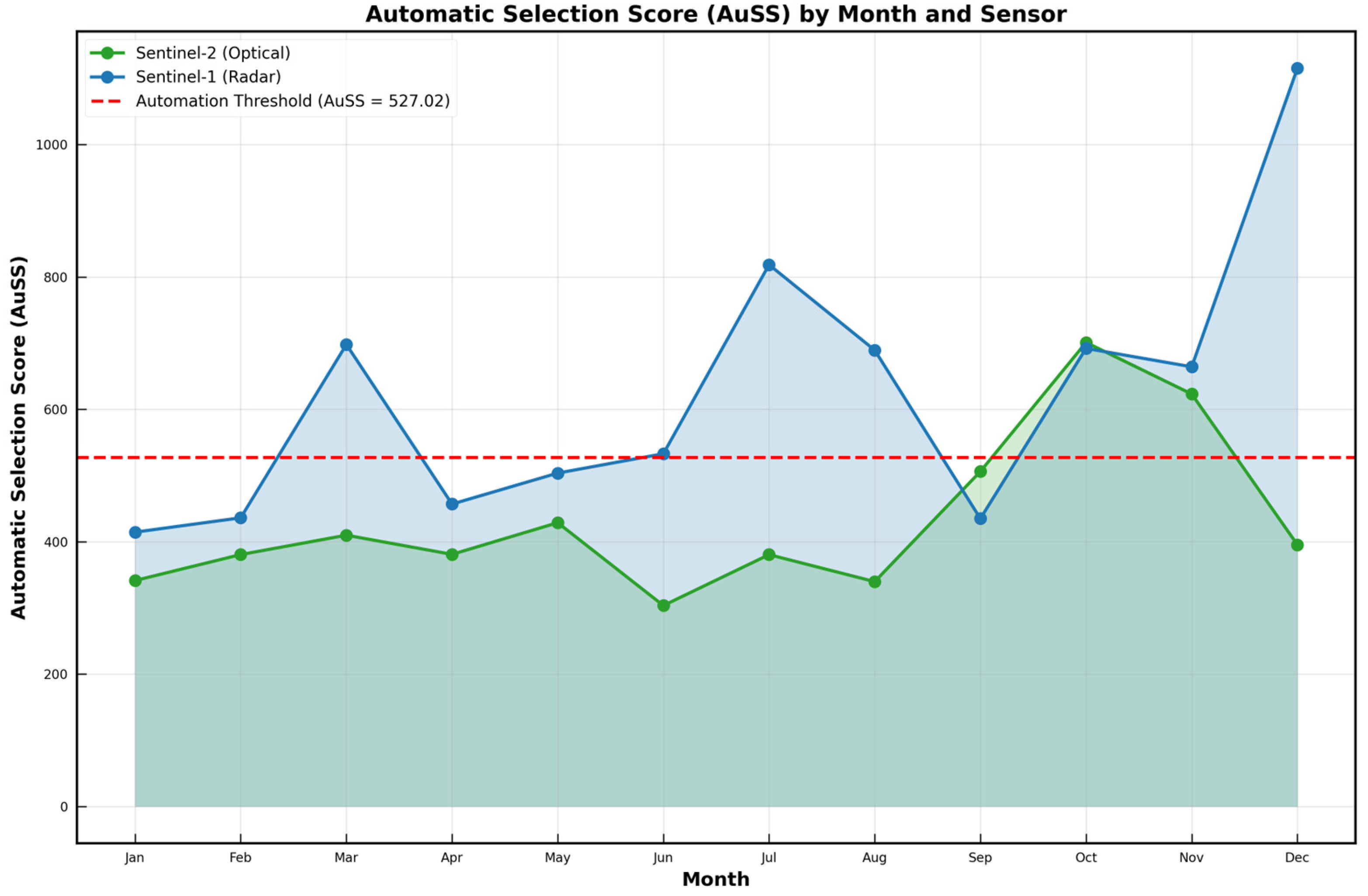
combines predictive importance with a logarithmic stability penalty. Figure 9 presents AuSS values by month for both sensor families, with the global automation threshold (mean AuSS = 527.0) indicated by a red dashed line.

Radar features maintain consistently high AuSS values throughout the agricultural season, frequently exceeding the threshold, with notable peaks observed in March (~700), mid-season (~800), and December (>1100). This indicates that radar-derived features combine strong predictive power with temporal robustness, making them suitable for automated use across most periods. In contrast, optical features exhibit a more variable pattern, remaining below the threshold for most of the season and exceeding it only during a limited period between September and November, with a peak around 700. This reflects their dependence on vegetation dynamics and acquisition conditions. These results further highlight the complementary roles of radar and optical data: radar provides a stable baseline for automated feature selection, while optical features contribute selectively during periods of increased discriminative power. The threshold therefore serves as a practical criterion for identifying features that are both informative and reliable across time.

The automation threshold (dashed red line) is set at the global mean AuSS across all months and sensor types (527.0). Features that consistently exceed this threshold are considered suitable for automated, zero-intervention use.

3.9. Feature Certainty and Entropy

Beyond stability and predictive importance, the clarity of the signal provided by each feature is critical for reducing model uncertainty in operational settings. To assess this aspect, we computed the information entropy of each index based on its normalized importance distribution across years. Lower entropy values indicate more consistent and less ambiguous behavior, while higher values reflect greater variability and uncertainty.

Table 15. Entropy-based robustness assessment of feature indices.

Index	Entropy	Stability (1/CV)	RI	Sensor
GNDVI	2.392	2.14	410.85	Optical
VV	2.429	2.87	1486.70	Radar
Ratio	2.433	2.934	841.64	Radar
VH	2.439	3.10	1631.65	Radar
EVI	2.440	3.14	1005.23	Optical
MSI	2.444	3.30	941.74	Optical
BSI	2.446	3.34	1171.46	Optical
NDVI	2.447	3.46	1459.51	Optical
GCVI	2.449	3.50	1349.95	Optical
RVI	2.449	3.65	1339.28	Radar
SAVI	2.450	3.66	1036.78	Optical
NDMI	2.460	4.25	855.50	Optical
NDRE	2.468	5.18	1782.93	Optical

summarizes the entropy values alongside stability and reliability metrics. The entropy values for all indices fall within a very narrow range (2.39–2.47) corresponding to a difference of only 0.08. This small range indicates that all features provide essentially the same level of informational consistency. No statistically meaningful difference is observed between indices (e.g., between GNDVI and NDRE). Therefore, we conclude that the Stable Portfolio maintains consistent prediction entropy across all selected indices; the observed variations are too small to be meaningfully interpreted. This consistency, rather than differences between indices, demonstrates that stability-driven selection reduces model uncertainty regardless of which index enters the portfolio.

Overall, entropy provides a complementary perspective on feature robustness, highlighting the trade-off between consistency and discriminative power in automated classification systems.

3.10. Voting Ensemble Performance with Stable Portfolio

Using the Stable Portfolio (6 indices) as input, we trained a Voting Ensemble (Random Forest, Extra Trees, XGBoost, and LightGBM) on 3773 training samples and evaluated it on 953 independent test samples. The results are summarized in

Table 16. Per-class performance of the Voting Ensemble using the Stable Portfolio.

Class	Precision	Recall	F1-Score	Support
Soft Wheat	0.90	0.91	0.90	225
Durum Wheat	0.88	0.89	0.88	158
Barley	0.86	0.87	0.86	154
Trees	0.91	0.90	0.90	179
Other Crops	0.90	0.89	0.90	237
Macro Average	0.89	0.89	0.89	953

. The model achieved an overall test accuracy of 87.4%, with a macro-averaged F1-score of 87.2%. Class-wise performance is consistently high across all crop types, with F1-scores ranging from 0.86 to 0.90, indicating balanced classification performance. The overfitting gap between training accuracy (94.8%) and cross-validation accuracy (88.6%) is limited to 6.2%, suggesting that the stability-driven feature selection effectively reduces sensitivity to year-specific variability.

3.11. Cross-Year Generalization and Statistical Significance

To evaluate temporal transferability, we compared the Stable Portfolio (72-feature set derived from the 6-index core: VH, VV, NDVI, NDRE, GCVI, RVI, each with 12 monthly values) against the full 156-feature set using the nine train-test combinations (training on one year, testing on all others).

Table 17. Cross-year generalization performance comparison.

Metric	Full Feature Set (156)	Stable Portfolio (72)	Improvement
Same-Year Accuracy	95.2%	94.8%	–0.4%
Cross-Year Accuracy	76.8%	84.3%	+7.5%
Generalization Gap	18.4%	10.5%	–7.9%
Worst-Case Accuracy	68.2%	81.7%	+13.5%
Consistency (1-std)	0.83	0.91	+0.08

reports the improvements achieved by the Stable Portfolio.

The generalization gap narrows from 18.4% to 10.5%, a 43% relative reduction, directly addressing the “temporal generalization gap” that continues to challenge operational remote sensing. The worst-case accuracy improves by 13.5%, providing a critical safety margin against anomalously challenging years.

Statistical significance was assessed with a Friedman test followed by Nemenyi post hoc comparisons (

Table 18. Statistical significance of performance differences (Nemenyi post hoc p-values).

Subset Comparison	p-Value	Significance
Stable Portfolio vs. Full Feature Set	0.003	**
Stable Portfolio vs. Volatile Set	<0.001	***
Stable Portfolio vs. Stable Set	0.042	*
Stable Portfolio vs. Top-RI Set	0.187	ns
Stable Portfolio vs. Top-AuSS Set	0.091	ns

Note: *** p < 0.001, ** p < 0.01, * p < 0.05, ns = not significant.

). The Friedman test revealed significant differences among subsets (χ² = 24.36, p < 0.001). The Stable Portfolio significantly outperforms both the Full Feature Set (p < 0.01) and the Volatile Set (p < 0.001), validating the effectiveness of stability-based selection. Non-significant differences with the Top-RI and Top-AuSS sets confirm that these metrics are effective selection criteria.

Together, these results demonstrate that the stability-driven framework identifies features capturing stable phenological signals rather than year-specific noise, enabling robust, climate-resilient crop classification.

3.12. Spatial Application and Stable Portfolio Validation

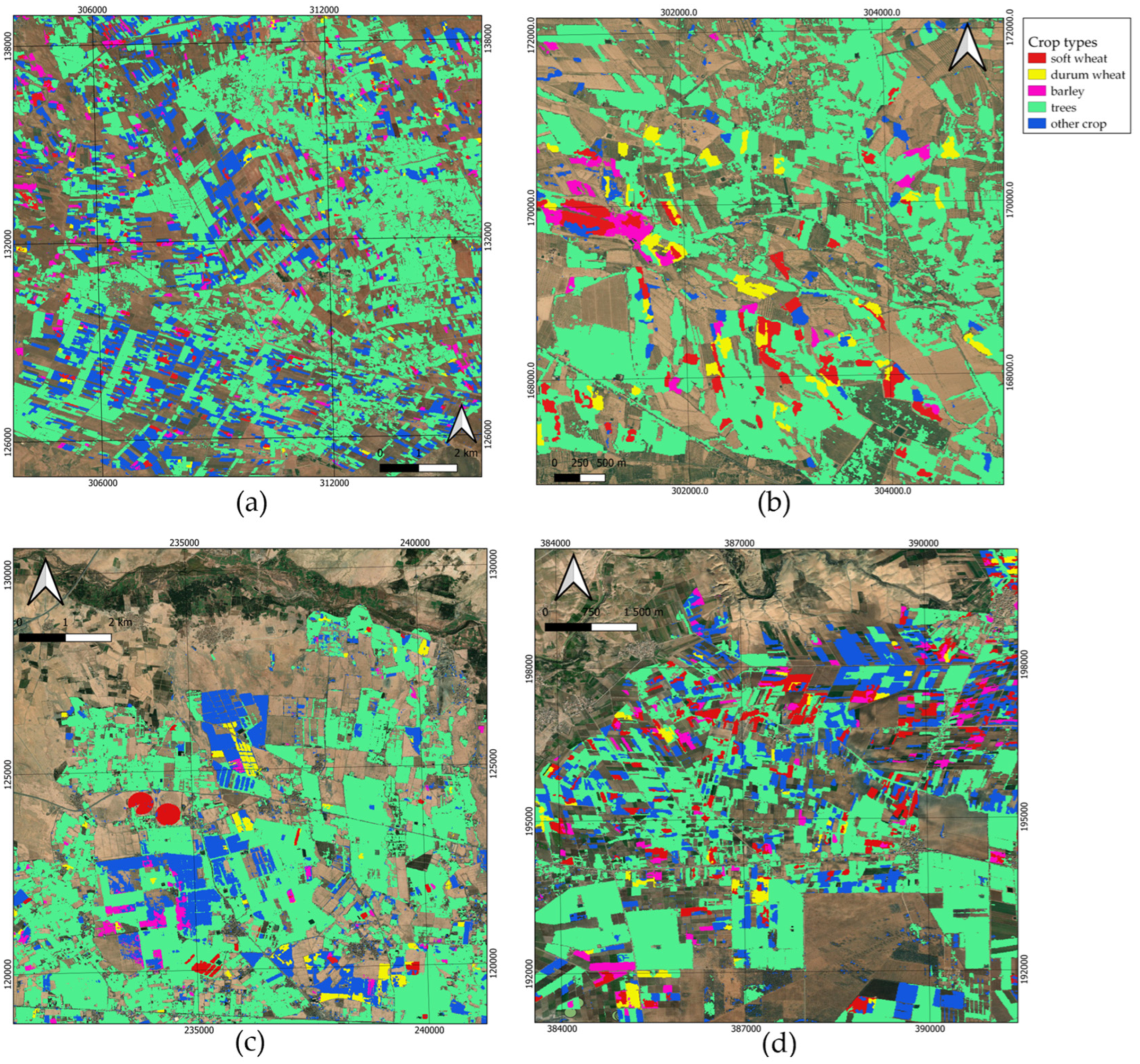
To evaluate the spatial transferability of the proposed framework, the Voting Ensemble classifier was applied to generate high-resolution (10 m) annual crop maps over four representative irrigated perimeters (Figure 10). The maps demonstrate the model’s ability to produce spatially coherent crop patterns across different agricultural landscapes.

In parallel, we assessed the impact of using a Stable Portfolio of features selected based on inter-annual stability (low coefficient of variation) as the sole input feature space. The Voting Ensemble trained on this Stable Portfolio achieved a test accuracy of 87.4% with a macro-averaged F1-score of 87.2% across the five crop classes (Table 15). Per-class F1-scores were 90.0% for Soft Wheat, 88.0% for Durum Wheat, 86.0% for Barley, 92% for Trees, and 90.0% for Other Crops, with an overfitting gap below 10%. Statistical significance of performance differences between feature subsets was assessed using paired t-tests and the non-parametric Friedman test with post hoc Nemenyi analysis (α = 0.05), confirming that the stability-driven feature selection does not compromise accuracy while enhancing model parsimony.

The spatial maps in Figure 10 are intended as a visual illustration of the Stable Portfolio’s outputs, not as a rigorous spatial validation. Detailed spatial accuracy assessment, including per-perimeter confusion matrices and area-level validation against official statistics, is provided in our companion paper focusing on classification benchmarking [43].

4. Discussion

4.1. The Importance-Stability Trade-Off: A Fundamental Constraint for Automation

This study demonstrates that feature importance in crop classification is fundamentally dynamic, and that the conventional paradigm of identifying a single “optimal” feature set from one or two years of data must be replaced by a stability-aware framework. Our analysis across six agricultural years (2018, 2019, 2020, 2023, 2024 and 2025) reveals a consistent and quantifiable trade-off: the most predictive features, notably optical indices during peak vegetation vigor (NDVI, GCVI) and radar backscatter (VH, VV), exhibit the highest inter-annual volatility, while the most stable features (NDRE, NDMI, MSI) offer only moderate predictive power [44,45]. This finding challenges the common assumption that a feature’s importance in a single year is a reliable indicator of its utility for long-term operational systems [46].

The four-quadrant behavioral typology (Figure 4) goes beyond simple ranking by offering a strategic decision framework: Dominant Stable indices (BSI, GCVI, NDRE, NDVI, RVI) become the core of an automated system; Performant Volatile indices (VH, VV) are used conditionally; Stable Minor indices (NDMI, SAVI) serve as structural anchors; and Noise/Unstable indices (EVI, GNDVI, MSI, Ratio) are pruned. This typology aligns with ecological theory that vegetation responses to climate are inherently dynamic and that effective remote sensing indicators must balance sensitivity to biophysical changes with resilience to inter-annual noise [47,48]. By aggregating importance estimates from four distinct tree-based algorithms (RF, ET, XGBoost, LightGBM), the Voting Ensemble consensus ensures that this typology reflects genuine phenological signals rather than algorithm-specific artifacts [49].

Critically, the typology reveals that no single feature excels in both criteria. This is not a limitation of our dataset but a fundamental property of remote sensing of vegetation: features that are highly sensitive to biophysical changes (e.g., NDVI at peak greenness) are inevitably also sensitive to the climatic drivers that cause inter-annual variability. Recognizing this trade-off forces a shift from optimizing for peak performance to designing for robustness, a concept well established in other domains (e.g., finance, engineering) but rarely applied in agricultural remote sensing.

4.2. Sensor Complementarity as the Key to Year-Round Automation

A key contribution of this study is the quantitative demonstration that Sentinel-1 radar and Sentinel-2 optical data are not redundant but fundamentally complementary [50]. The consistently low cross-correlation between the two families (|ρ| < 0.3, Figure 3) confirms that they capture orthogonal aspects of crop canopies: radar responds to dielectric properties and canopy geometry, while optical indices track chlorophyll content and leaf area index [51]. This complementarity is often assumed but rarely quantified with multi-year data.

More importantly, the temporal trajectory (Figure 5) and the AuSS by month (Figure 9) reveal when each sensor should dominate an automated pipeline. Radar maintains high importance and high AuSS throughout the year, with peaks in March, July, and December, periods corresponding to early growth, mid-season stress detection, and harvest. Optical indices, in contrast, become critical only during September–November, the post-harvest window. This pattern provides a direct operational rule: during sowing, growth, and harvest, rely on radar’s stability; during the narrow phenological window where optical indices exceed the automation threshold, integrate them for their high discriminative power. This phenologically adaptive strategy is a departure from static sensor-weighting approaches [52,53] and is essential for achieving year-round reliability.

The robustness fingerprint (Figure 6) further quantifies this complementarity: radar excels in stability, availability, timeliness, and weather independence, while optical indices dominate only in predictive importance. This profile reinforces the concept of a robust baseline (radar) combined with a high-resolution but conditionally applied sensor (optical)—a design that is both theoretically grounded and practically feasible [54,55]. In the context of operational monitoring, such a design reduces the risk of system failure during periods of cloud cover or atmospheric disturbances, a common problem in Mediterranean climates.

4.3. The Stable Portfolio: A Pareto-Optimal Foundation for Automation

Pareto optimization (Figure 8) shows that 6 indices—VH, VV, NDVI, NDRE, GCVI, RVI—capture 57.2% of cumulative importance, while the remaining 7 indices contribute a marginal additional signal. This 54% reduction in the number of indices (from 13 to 6) demonstrates that conventional full-feature approaches carry substantial redundancy and overfitting risk [56,57]. The Stable Portfolio identified by this method is not merely a subset; it is a balanced ensemble that includes three radar indices (VH, VV, RVI) and three optical indices (NDVI, NDRE, GCVI), reflecting the sensor complementarity discussed above.

Unlike conventional feature selection that maximizes within-year accuracy [58], our Automatic Selection Score (AuSS) explicitly balances predictive importance with a logarithmic stability penalty, ensuring that selected features are both powerful and reliable across diverse climatic years. The Reliability Index (RI) provides an even more direct measure of this trade-off and ranks NDRE, VH, and VV as the top three pillars (Table 13). The entropy analysis (Figure 8) adds an additional layer: low-entropy features (NDRE, NDMI, SAVI) provide unambiguous signatures that ground the model’s decisions, reducing vulnerability to edge cases and atmospheric perturbations [59]. Together, RI, AuSS, and entropy form a multi-dimensional screening process that yields a portfolio optimized for operational deployment. Similar dimensionality reductions have been successfully applied in large-area crop mapping [60].

Importantly, the Stable Portfolio is not merely a list of indices; it is a dynamic concept. The inclusion of both radar and optical indices, and the explicit use of monthly composites, means that the portfolio inherently captures the phenological shifts in feature importance. This is a departure from static feature sets that are applied uniformly across the entire season.

4.4. The Automated Model: Voting Ensemble with Stable Portfolio

The Voting Ensemble trained on the Stable Portfolio achieved 87.4% test accuracy and a macro-averaged F1-score of 87.2% across five crop classes (Table 15). Critically, the per-class performance is balanced (F1 ranging from 0.86 for Barley to 0.90 for Soft Wheat, Trees, and Other Crops), indicating that the Stable Portfolio captures discriminative information for all classes without favoring spectrally distinct ones [52]. The slight underperformance of Barley reflects its higher phenological plasticity and wider cultivation range, factors that increase intra-class spectral variability, a known challenge in Mediterranean environments [61].

The primary misclassifications occurred between spectrally similar classes (Durum Wheat/Soft Wheat, Trees/Other Crops), a pattern consistent with the inherent spectral similarity of these categories [62]. This suggests that further improvements may require additional data sources (e.g., time-series phenological metrics) rather than more feature engineering within the current sensor suite. It also highlights that the Stable Portfolio, while robust, does not eliminate all confusion; rather, it focuses on features that are stable and generally discriminative, accepting that some spectral overlap is unavoidable without additional information.

Most importantly, the overfitting gap between training (94.8%) and cross-validation (88.6%) accuracy is only 6.2%, suggesting that stability-driven feature selection effectively eliminates year-specific noise [63]. This low gap is a direct consequence of using the Stable Portfolio and demonstrates that the model is not memorizing climatic anomalies but learning persistent phenological relationships.

4.5. Solving the Temporal Generalization Gap

The cross-year validation results (Table 17) provide the strongest evidence for the operational value of our framework. The Stable Portfolio achieves 84.3% cross-year accuracy compared to 76.8% for the full feature set, representing a 7.5% absolute improvement. More importantly, the generalization gap narrows from 18.4% to 10.5%, a 43% relative reduction. This directly addresses the “temporal generalization gap” that has long been recognized as a fundamental obstacle in operational remote sensing [64,65].

Models trained on the full feature set capture year-specific patterns that fail to transfer, as reflected in their high same-year accuracy (95.2%) but poor cross-year performance. In contrast, the Stable Portfolio, by focusing on features with proven multi-year stability, captures underlying phenological signals that persist across climatic variations [66]. The worst-case accuracy improvement from 68.2% to 81.7% is particularly significant for operational systems, where reliability under challenging conditions often matters more than peak performance. This 13.5% gain provides a critical safety margin against anomalous years, reducing the risk of catastrophic failure when deploying automated systems in new environments [67].

Statistical significance testing (Table 17) confirms that these improvements are not due to chance. The Stable Portfolio significantly outperforms the Full Feature Set (p < 0.01) and the Volatile Set (p < 0.001), while the non-significant differences with the Top-RI and Top-AuSS sets validate that these metrics are effective selection criteria. The marginal significance of the Stable Set (p < 0.05) suggests that pure stability without importance weighting is insufficient, a key insight that justifies the composite nature of RI and AuSS.

4.6. A Pathway to Less-Intervention Operational Mapping

This study provides a complete, replicable pathway from raw satellite data to a fully automated, climate-resilient classification system. The framework begins with multi-year consensus importance derived from a Voting Ensemble, which filters out algorithm-specific noise and reveals stable phenological signals [68]. Stability metrics (CV, Stability Index) quantify inter-annual consistency, while the novel composite indices RI and AuSS balance importance with stability, providing actionable selection criteria [69,70]. Pareto optimization identifies the minimal feature set (6 indices, 57.2% of cumulative importance), and the final Voting Ensemble trained on this Stable Portfolio achieves high accuracy with a minimal generalization gap.

The resulting system significantly reduces the manual intervention for feature selection or model retraining across years [71]. The Stable Portfolio was identified once using historical data (2018, 2019, 2020, 2023, 2024 and 2025) and transfers effectively to new years without modification. This represents a fundamental shift from the current practice of annual model retraining and feature re-optimization [72,73], and it is precisely the kind of approach needed to scale satellite-based crop monitoring to operational levels. The potential cost savings in reduced ground data requirements and computational overhead could be substantial, and the increased reliability makes the system suitable for integration into national monitoring programs [74].

Our framework was developed and validated on five irrigation zones with a Mediterranean winter cropping system (sowing September–November). Morocco also has Atlantic zones (cooler, wetter, earlier sowing) and pre-Saharan zones (arid, summer cropping). While we did not test these zones, the framework can be adapted by: (1) shifting monthly composites to match local phenology or (2) retraining stability metrics with 2–3 years of local data. Future work will validate this transferability.

Moreover, the framework is transferable. While the specific Stable Portfolio was derived for Morocco’s cereal-dominated landscapes, the methodology, multi-year ensemble consensus, stability metrics, and Pareto optimization can be applied to any region and any crop type. The demonstrated patterns of sensor complementarity (radar stable year-round, optical peak in autumn) are likely to hold in other Mediterranean and semi-arid environments, though regional calibration would be beneficial.

4.7. Limitations and Future Research Directions

While this study provides comprehensive insights into feature stability, several limitations should be acknowledged. Although the six-year analysis period is substantial, it represents a specific climatic window in Morocco; the gap between 2020 and 2023 means that certain inter-annual variability patterns may not be fully captured. As shown by Forkel et al. [75], even gaps of 2–3 years can affect breakpoint detection performance, particularly for gradual trend changes, suggesting our stability estimates may be conservative. Extending this analysis to longer time series and different agro-ecological zones would validate the generalizability of the Stable Portfolio and the stability metrics [76].

Second, the focus on cereal crops in Morocco’s Mediterranean climate means the specific feature rankings may not transfer directly to other cropping systems or climatic regimes. However, the methodological framework, Voting Ensemble consensus, stability metrics, and Pareto optimization, is designed to be transferable, and similar patterns of sensor complementarity likely apply across agricultural systems [77,78]. Future work should test the framework in regions with different crop types (e.g., root crops, orchards) and climatic conditions (e.g., humid tropics, temperate zones).

Third, we used only raw radar backscatter (VV, VH) and derived indices (VH/VV, RVI). Future work should investigate whether other SAR metrics (e.g., polarimetric decompositions, coherence) offer different stability-importance trade-offs [78]. Similarly, the inclusion of additional optical indices (e.g., those sensitive to canopy water content or lignin) could further refine the portfolio.

Fourth, the Voting Ensemble, while robust, requires more computational resources than single classifiers. For very large-scale operational deployment, investigating lighter models (e.g., distilled versions of the ensemble, or simpler models like logistic regression with the Stable Portfolio) that maintain the generalization would be valuable.

Future research directions include:

• Integration of meteorological data to understand the environmental drivers of feature volatility and develop conditional models that adapt to predicted climate anomalies. For example, in years forecasted to be dry, the model could automatically increase the weight of water stress indices.
• Temporal transfer learning approaches that fine-tune the Stable Portfolio with minimal new data each year rather than retraining from scratch. This could further reduce operational costs. Also, Iterative decomposition methods such as BFAST could inform this process by identifying when seasonal or trend components shift significantly [79].
• Extension to other crop types and regions to validate the universality of the importance-stability trade-off and the effectiveness of the AuSS metric.
• Deep learning architectures that can automatically learn stable feature representations, potentially identifying patterns not captured by hand-crafted indices. Such architectures could directly output stability-weighted features, bypassing the manual index engineering step.
• Operational deployment studies that test the Stable Portfolio-based Voting Ensemble in real-time mapping scenarios, measuring not just accuracy but also computational efficiency and reliability under operational constraints (e.g., cloud cover, data latency).

5. Conclusions

This study demonstrates that feature importance in crop classification is fundamentally dynamic, and that stability-aware feature selection is not merely diagnostic but essential for operational automation. Through a comprehensive analysis of 156 multi-sensor features across six agricultural years in Morocco, using Voting Ensemble consensus to derive robust importance estimates, we have established several key findings with both scientific and practical significance. While the framework demonstrates strong performance across five irrigation zones, full national operational capability would require validation in additional agro-ecological zones (e.g., Atlantic and pre-Saharan regions) and sensitivity analysis of the automation threshold across these zones. Nevertheless, the methodology is transferable, and the Stable Portfolio provides a robust foundation for scaling to national monitoring with modest local calibration

First, we quantified the fundamental importance-stability trade-off that governs feature utility in multi-annual crop mapping. The four-quadrant behavioral typology comprising Dominant Stable, High-Performing Volatile, Stable Minor, and Noise provides a strategic framework for understanding this trade-off and making informed feature selection decisions. No feature excels in both criteria, confirming that operational systems must balance rather than optimize.

Second, we demonstrated the complementary roles of Sentinel-1 radar and Sentinel-2 optical data across the phenological cycle. Radar provides exceptional stability throughout the year, with peaks in early growth, mid-season stress detection, and harvest, serving as the structural backbone of automated systems. Optical vegetation indices dominate during the post-harvest period (September–November), providing irreplaceable discriminative power despite their higher volatility. This complementarity enables year-round automation through adaptive, phenology-aware sensor weighting.

Third, we introduced novel composite indices—the Reliability Index (RI) and Automatic Selection Score (AuSS)—that explicitly balance predictive importance with temporal stability. These metrics provide actionable criteria for feature selection, identifying the pillars of automation that perform consistently across diverse climatic conditions.

Fourth, we applied Pareto optimization to identify a Stable Portfolio of six indices—VH, VV, NDVI, NDRE, GCVI, and RVI—which captures 57.2% of cumulative predictive importance while filtering out inter-annual noise. This 54% reduction in the number of indices demonstrates that conventional full-feature approaches carry substantial redundancy and overfitting risk.

Fifth and most significantly, we validated that the Voting Ensemble trained on this Stable Portfolio achieves operational readiness. With 87.4% test accuracy, 87.2% macro F1-score, and a generalization gap of only 10.5% (compared to 18.4% for the full feature set), this model is capable of year-to-year transfer with minimal intervention. The 13.5% improvement in worst-case accuracy provides a critical safety margin against anomalous years and directly helps address the temporal generalization gap that has long hindered operational remote sensing.

This work has several practical implications, operational systems can adopt the Stable Portfolio of six indices as a foundation, eliminating the need for annual feature re-optimization. They can implement the Voting Ensemble combining Random Forest, Extra Trees, XGBoost, and LightGBM as the classifier, leveraging multi-model consensus for robust predictions. They can use the Automatic Selection Score threshold of 527 as a guideline for incorporating new features, ensuring that additions meet stability criteria. They can apply the cross-year validation protocol as a standard practice, recognizing that same-year accuracy overestimates operational performance. And they can leverage sensor complementarity by trusting radar during transition phases and optical indices during their peak windows, adapting weights phenologically.

From a broader perspective, this work challenges the conventional paradigm of static feature selection in remote sensing. The features that appear most important in single-year studies are often the most volatile, optimizing for historical performance rather than future robustness. By shifting focus from importance alone to the importance-stability trade-off, and by providing the quantitative tools of the Reliability Index and Automatic Selection Score to manage this trade-off, we enable a new generation of automated classification systems designed for resilience rather than peak performance.

The framework developed here, encompassing Voting Ensemble consensus importance, stability metrics, Pareto-optimized portfolio, and final ensemble validation is transferable to other regions, crop types, and sensor combinations. As climate variability increases and the demand for timely agricultural information grows, such stability-aware approaches will become essential for building monitoring systems that remain reliable in the face of environmental change. Future work should extend this analysis to longer time series, integrate meteorological drivers of volatility, and explore deep learning architectures that can automatically learn stable feature representations. Fully automated, climate-resilient crop mapping at scale is now an achievable goal, guided by the principles and tools established in this study.

The complete code for feature extraction, stability analysis, Pareto optimization, and model training is available in a Jupyter notebook at the following anonymized repository: https://colab.research.google.com/drive/1xgGF35OakpoCxuPqiwOoxNO7YT20CcNp?usp=sharing (accessed on 18 June 2026). The repository includes all preprocessing steps, hyperparameter configurations, and instructions for reproducing the results.

References

1. Haider, K.; Abbas, D.; Ullah, F.; Ijaz, M.; Ikram, M.; Kabir, K.; Khan, K.A.; Galian, J. Climate-driven insect pest outbreaks and food security risks: A review of adaptive strategies for resilient agriculture. J. Pest Sci. 2026, 99, 12. [Google Scholar] [CrossRef]
2. Yu, L.; Du, Z.; Li, X.; Zheng, J.; Zhao, Q.; Wu, H.; Weise, D.; Yang, Y.; Zhang, Q.; Li, X.; et al. Enhancing global agricultural monitoring system for climate-smart agriculture. Clim. Smart Agric. 2025, 2, 100037. [Google Scholar] [CrossRef]
3. Choukri, M.; Laamrani, A.; Chehbouni, A. Use of optical and radar imagery for crop type classification in Africa: A review. Sensors 2024, 24, 3618. [Google Scholar] [CrossRef] [PubMed]
4. Misbah, K.; Laamrani, A.; Khechba, K.; Dhiba, D.; Chehbouni, A. Multi-sensors remote sensing applications for assessing, monitoring, and mapping NPK content in soil and crops in African agricultural land. Remote Sens. 2021, 14, 81. [Google Scholar] [CrossRef]
5. Khechba, K.; Laamrani, A.; Dhiba, D.; Misbah, K.; Chehbouni, A. Monitoring and analyzing yield gap in Africa through soil attribute best management using remote sensing approaches: A review. Remote Sens. 2021, 13, 4602. [Google Scholar] [CrossRef]
6. Tuia, D.; Persello, C.; Bruzzone, L. Recent advances in domain adaptation for the classification of remote sensing data. arXiv 2021, arXiv:2104.07778. [Google Scholar] [CrossRef]
7. Li, S.; Liu, L.; Huo, J.; Li, S.; Yin, Y.; Ma, Y. A Class-Aware Unsupervised Domain Adaptation Framework for Cross-Continental Crop Classification with Sentinel-2 Time Series. Remote Sens. 2025, 17, 3762. [Google Scholar] [CrossRef]
8. Nyborg, J.; Pelletier, C.; Lefèvre, S.; Assent, I. TimeMatch: Unsupervised cross-region adaptation by temporal shift estimation. ISPRS J. Photogramm. Remote Sens. 2022, 188, 301–313. [Google Scholar] [CrossRef]
9. Huang, J.; Xiao, G.; Li, X.; Zheng, J.; Zeng, Y.; Su, W.; Miao, S.; Gobin, A. Progress and Perspectives of Crop Type Mapping With Remote Sensing: A review. IEEE Geosci. Remote Sens. Mag. 2026, 14, 129–162. [Google Scholar] [CrossRef]
10. El Bouanani, N.; Laamrani, A.; Hajji, H.; Bourriz, M.; Bourzeix, F.; Ait Abdelali, H.; El-Battay, A.; Amazirh, A.; Chehbouni, A. Estimating soil attributes for yield gap reduction in Africa using hyperspectral remote sensing data with artificial intelligence methods: An extensive review and synthesis. Remote Sens. 2025, 17, 1597. [Google Scholar] [CrossRef]
11. Thingujam, U.; Prabha, D.; Ghosh Bag, A.; Thingujam, V.; Darshan, N.P.; Dutta, S.; Gorain, S. From point sensing to intelligent systems: A comprehensive review on advanced sensor technologies for soil health monitoring. Discov. Sens. 2025, 1, 27. [Google Scholar] [CrossRef]
12. Zhang, Z.; Huang, L.; Wang, Q.; Jiang, L.; Qi, Y.; Wang, S.; Shen, T.; Tang, B.-H.; Gu, Y. UAV hyperspectral remote sensing image classification: A systematic review. IEEE J. Sel. Top. Appl. Earth Obs. Remote Sens. 2024, 18, 3099–3124. [Google Scholar] [CrossRef]
13. Zhao, P.; Hu, W.; Cao, D.; Dong, Z.; Zeng, Y.; Huang, Q.; Chen, Z. A Review on Deep Learning-Based Electrical Load Forecasting: From Perspectives of Learning Paradigms and Foundation Models. J. Mod. Power Syst. Clean Energy 2026, 14, 791–809. [Google Scholar] [CrossRef]
14. Peña-Barragán, J.M.; Ngugi, M.K.; Plant, R.E.; Six, J. Object-based crop identification using multiple vegetation indices, textural features and crop phenology. Remote Sens. Environ. 2011, 115, 1301–1316. [Google Scholar] [CrossRef]
15. Laamrani, A.; Berg, A.A.; Voroney, P.; Feilhauer, H.; Blackburn, L.; March, M.; Dao, P.D.; He, Y.; Martin, R.C. Ensemble identification of spectral bands related to soil organic carbon levels over an agricultural field in Southern Ontario, Canada. Remote Sens. 2019, 11, 1298. [Google Scholar] [CrossRef]
16. Badshah, A.; Alkazemi, B.Y.; Din, F.; Zamli, K.Z.; Haris, M. Crop classification and yield prediction using robust machine learning models for agricultural sustainability. IEEE Access 2024, 12, 162799–162813. [Google Scholar] [CrossRef]
17. Ouzemou, J.E.; El Harti, A.; Lhissou, R.; El Moujahid, A.; Bouch, N.; El Ouazzani, R.; Bachaoui, E.M.; El Ghmari, A. Crop type mapping from pansharpened Landsat 8 NDVI data: A case of a highly fragmented and intensive agricultural system. Remote Sens. Appl. Soc. Environ. 2018, 11, 94–103. [Google Scholar] [CrossRef]
18. Orynbaikyzy, A.; Gessner, U.; Mack, B.; Conrad, C. Crop type classification using fusion of sentinel-1 and sentinel-2 data: Assessing the impact of feature selection, optical data availability, and parcel sizes on the accuracies. Remote Sens. 2020, 12, 2779. [Google Scholar] [CrossRef]
19. Büyükkeçeci, M.; Okur, M.C. A comprehensive review of feature selection and feature selection stability in machine learning. Gazi Univ. J. Sci. 2023, 36, 1506–1520. [Google Scholar] [CrossRef]
20. Miao, Y.; Mulla, D.J.; Robert, P.C. Identifying important factors influencing corn yield and grain quality variability using artificial neural networks. Precis. Agric. 2006, 7, 117–135. [Google Scholar] [CrossRef]
21. Werner, C.; Schnyder, H.; Cuntz, M.; Keitel, C.; Zeeman, M.J.; Dawson, T.E.; Badeck, F.-W.; Brugnoli, E.; Ghashghaie, J.; Grams, T.E.E.; et al. Progress and challenges in using stable isotopes to trace plant carbon and water relations across scales. Biogeosciences 2012, 9, 3083–3111. [Google Scholar] [CrossRef]
22. Ouzemou, J.E.; El Harti, A.; Moujahid, A.E.; Bouch, N.; El Ouazzani, R.; Lhissou, R.; Bachaoui, E.M. Mapping crop based on phenological characteristics using time-series NDVI of operational land imager data in Tadla irrigated perimeter, Morocco. In Proceedings of the Remote Sensing for Agriculture, Ecosystems, and Hydrology XVII, Toulouse, France, 22–24 September 2015; SPIE: Paris, France, 2015; Volume 9637, p. 96372G. [Google Scholar] [CrossRef]
23. Heiss, N.; Meier, J.; Gessner, U.; Kuenzer, C. A review: Potential of Earth observation (EO) for mapping Small-Scale agriculture and cropping systems in West Africa. Land 2025, 14, 171. [Google Scholar] [CrossRef]
24. Ahmed, S.; Mahmoud, A.S.; Farg, E.; Mohamed, A.M.; Moustafa, M.S.; Abutaleb, K.; Saleh, A.M.; AbdelRahman, M.A.; AbdelSalam, H.M.; Arafat, S.M. Investigation on the use of ensemble learning and big data in crop identification. Heliyon 2023, 9, e13339. [Google Scholar] [CrossRef] [PubMed]
25. Kierdorf, J.; Roscher, R. Reliability scores from saliency map clusters for improved image-based harvest-readiness prediction in cauliflower. IEEE Geosci. Remote Sens. Lett. 2023, 20, 8500505. [Google Scholar] [CrossRef]
26. Coluzzi, R.; Imbrenda, V.; Lanfredi, M.; Simoniello, T. A first assessment of the Sentinel-2 Level 1-C cloud mask product to support informed surface analyses. Remote Sens. Environ. 2018, 217, 426–443. [Google Scholar] [CrossRef]
27. Lebrini, Y.; Boudhar, A.; Laamrani, A.; Htitiou, A.; Lionboui, H.; Salhi, A.; Chehbouni, A.; Benabdelouahab, T. Mapping and characterization of phenological changes over various farming systems in an arid and semi-arid region using multitemporal moderate spatial resolution data. Remote Sens. 2021, 13, 578. [Google Scholar] [CrossRef]
28. Achli, S.; Ongoma, V.; Epule, T.E.; Dhiba, D.; Salih, W.; Ousayd, L.; Chehbouni, A. Exploring the key drivers of crop yields in Morocco–a systematic review. Front. Agron. 2025, 7, 1515938. [Google Scholar] [CrossRef]
29. Verbesselt, J.; Hyndman, R.; Newnham, G.; Culvenor, D. Detecting trend and seasonal changes in satellite image time series. Remote Sens. Environ. 2010, 114, 106–115. [Google Scholar] [CrossRef]
30. Solymosi, K.; Kövér, G.; Romvári, R. The development of vegetation indices: A short overview. Acta Agrar. Kaposváriensis 2019, 23, 75–90. [Google Scholar] [CrossRef]
31. Zhang, L.; Zhang, Z.; Luo, Y.; Cao, J.; Xie, R.; Li, S. Integrating satellite-derived climatic and vegetation indices to predict smallholder maize yield using deep learning. Agric. For. Meteorol. 2021, 311, 108666. [Google Scholar] [CrossRef]
32. Dapke, P.P.; Nagare, S.M.; Quadri, S.A.; Bandal, S.B.; Gaikwad, R.M.; Baheti, M.R. Seasonal analysis of vegetation, moisture, urbanization, and Land Surface Temperature (LST) using NDVI, NDMI, NDWI, and NDBI indices: A case study of sillod, Maharashtra. In Proceedings of the 2025 International Conference on Computational, Communication and Information Technology (ICCCIT), Indore, India, 7–8 February 2025; pp. 753–760. [Google Scholar] [CrossRef]
33. Vera-Esmeraldas, A.; Pizarro-Oteíza, S.; Labbé, M.; Rojo, F.; Salazar, F. UAV-Based Spectral and Thermal Indices in Precision Viticulture: A Review of NDVI, NDRE, SAVI, GNDVI, and CWSI. Agronomy 2025, 15, 2569. [Google Scholar] [CrossRef]
34. Nguyen, C.T.; Chidthaisong, A.; Kieu Diem, P.; Huo, L.-Z. A Modified Bare Soil Index to Identify Bare Land Features during Agricultural Fallow-Period in Southeast Asia Using Landsat 8. Land 2021, 10, 231. [Google Scholar] [CrossRef]
35. Kobayashi, N.; Tani, H.; Wang, X.; Sonobe, R. Crop classification using spectral indices derived from Sentinel-2A imagery. J. Inf. Telecommun. 2020, 4, 67–90. [Google Scholar] [CrossRef]
36. Mandal, D.; Ratha, D.; Bhattacharya, A.; Kumar, V.; McNairn, H.; Rao, Y.S.; Frery, A.C. A radar vegetation index for crop monitoring using compact polarimetric SAR data. IEEE Trans. Geosci. Remote Sens. 2020, 58, 6321–6335. [Google Scholar] [CrossRef]
37. He, S.; Peng, P.; Chen, Y.; Wang, X. Multi-crop classification using feature selection-coupled machine learning classifiers based on spectral, textural and environmental features. Remote Sens. 2022, 14, 3153. [Google Scholar]
38. Thinn, K.T.; Saeed, W. Consensus and Divergence in Explainable AI (XAI): Evaluating Global Feature-Ranking Consistency with Empirical Evidence from Solar Energy Forecasting. Mathematics 2026, 14, 297. [Google Scholar] [CrossRef]
39. Wang, L.; Dong, Q.; Yang, L.; Gao, J.; Liu, J. Crop classification based on a novel feature filtering and enhancement method. Remote Sens. 2019, 11, 455. [Google Scholar] [CrossRef]
40. Belgiu, M.; Drăguţ, L. Random forest in remote sensing: A review of applications and future directions. ISPRS J. Photogramm. Remote Sens. 2016, 114, 24–31. [Google Scholar] [CrossRef]
41. Wang, Z.; Zhang, C.; Gao, L.; Fan, C.; Xu, X.; Zhang, F.; Zhou, Y.; Niu, F.; Li, Z. Time phase selection and accuracy analysis for predicting winter wheat yield based on time series vegetation index. Remote Sens. 2024, 16, 1995. [Google Scholar] [CrossRef]
42. Liang, J.; Sawut, M.; Cui, J.; Hu, X.; Xue, Z.; Zhao, M.; Zhang, X.; Rouzi, A.; Ye, X.; Xilike, A. Object-oriented multi-scale segmentation and multi-feature fusion-based method for identifying typical fruit trees in arid regions using Sentinel-1/2 satellite images. Sci. Rep. 2024, 14, 18230. [Google Scholar] [CrossRef] [PubMed]
43. Choukri, M.; Bouroubi, Y.; Ouzemou, J.-E.; Grich, S.; Kamga Fotso, G.A.; Ojaghi, S.; Chehbouni, A.; Laamrani, A. A Mul-ti-Class, Multi-Temporal Crop and Land Cover Mapping Framework for Morocco Using Sentinel-1/2 Monthly Composites and Advanced Machine Learning Ensembles. Front. Remote Sens. 2026; under review.
44. Gao, Z.; Guo, D.; Ryu, D.; Western, A.W. Training sample selection for robust multi-year within-season crop classification using machine learning. Comput. Electron. Agric. 2023, 210, 107927. [Google Scholar] [CrossRef]
45. Fastovich, D.; Meyers, S.R.; Saupe, E.E.; Williams, J.W.; Dornelas, M.; Dowding, E.M.; Finnegan, S.; Huang, H.-H.M.; Jonkers, L.; Kiessling, W.; et al. Coupled, decoupled, and abrupt responses of vegetation to climate across timescales. Science 2025, 389, 64–68. [Google Scholar] [CrossRef] [PubMed]
46. Ezzahar, J.; Chehbouni, A.; Ouaadi, N.; Madiafi, M.; Said, K.; Er-Raki, S.; Laamrani, A.; Chakir, A.; Chabaane, Z.L.; Zribi, M. Sentinel-1 backscatter and interferometric coherence for soil moisture retrieval in winter wheat fields within a semiarid south-mediterranean climate: Machine learning versus semiempirical models. IEEE J. Sel. Top. Appl. Earth Obs. Remote Sens. 2023, 17, 2256–2271. [Google Scholar] [CrossRef]
47. Li, Z.; Xu, D.; Guo, X. Remote sensing of ecosystem health: Opportunities, challenges, and future perspectives. Sensors 2014, 14, 21117–21139. [Google Scholar] [CrossRef] [PubMed]
48. Tian, Y.; Zeng, T.; Lü, Q.; Jiang, H.; Yang, S.; Cao, H.; Yu, W. Multi-Source Remote Sensing Data-Driven Susceptibility Mapping of Retrogressive Thaw Slumps in the Yangtze River Source Region. Remote Sens. 2026, 18, 380. [Google Scholar] [CrossRef]
49. Tsai, Y.L.S.; Lin, S.Y.; Kim, J.R.; Choi, Y. Analysis of the seasonal velocity difference of the Greenland Russell glacier using multi-sensor data. Terr. Atmos. Ocean. Sci. 2019, 30, 541–562. [Google Scholar] [CrossRef]
50. Gholizadeh, A.; Kopačková, V. Detecting vegetation stress as a soil contamination proxy: A review of optical proximal and remote sensing techniques. Int. J. Environ. Sci. Technol. 2019, 16, 2511–2524. [Google Scholar] [CrossRef]
51. Steele-Dunne, S.C.; McNairn, H.; Monsivais-Huertero, A.; Judge, J.; Liu, P.W.; Papathanassiou, K. Radar remote sensing of agricultural canopies: A review. IEEE J. Sel. Top. Appl. Earth Obs. Remote Sens. 2017, 10, 2249–2273. [Google Scholar] [CrossRef]
52. Sun, Z.; Wang, D.; Zhong, G. A Review of Crop Classification Using Satellite-Based Polarimetric SAR Imagery. In Proceedings of the 2018 7th International Conference on Agro-Geoinformatics (Agro-Geoinformatics), Hangzhou, China, 6–9 August 2018; pp. 1–5. [Google Scholar] [CrossRef]
53. Nestola, E.; Scartazza, A.; Di Baccio, D.; Castagna, A.; Ranieri, A.; Cammarano, M.; Mazzenga, F.; Matteucci, G.; Calfapietra, C. Are optical indices good proxies of seasonal changes in carbon fluxes and stress-related physiological status in a beech forest? Sci. Total Environ. 2018, 612, 1030–1041. [Google Scholar] [CrossRef] [PubMed]
54. Guan, X.; Liu, M.; Cao, S.; Jiang, J. Phenology-Aware Transformer for Semantic Segmentation of Non-Food Crops from Multi-Source Remote Sensing Time Series. Remote Sens. 2025, 17, 2346. [Google Scholar] [CrossRef]
55. Kang, K.; Xie, J.; Liu, X.; Wang, H. Overview of the application of intelligent optimization algorithms in multi-attribute group decision making. Appl. Intell. 2025, 55, 409. [Google Scholar] [CrossRef]
56. Hu, K.; Wang, Z.; Coleman, G.; Bender, A.; Yao, T.; Zeng, S.; Song, D.; Schumann, A.; Walsh, M. Deep learning techniques for in-crop weed recognition in large-scale grain production systems: A review. Precis. Agric. 2024, 25, 1–29. [Google Scholar] [CrossRef]
57. Pour, N.G.; Shemehsavar, S. DCB-VIM: An ensemble learning based filter method for feature selection with imbalanced class distribution. Neurocomputing 2025, 651, 130848. [Google Scholar] [CrossRef]
58. Wei, Y.; Guo, X.; Lu, Y.; Hu, H.; Wang, F.; Li, R.; Li, X. Phenology-Guided Wheat and Corn Identification in Xinjiang: An Improved U-Net Semantic Segmentation Model Using PCA and CBAM-ASPP. Remote Sens. 2025, 17, 3563. [Google Scholar] [CrossRef]
59. Li, L.; Zhu, Z.; Wang, C. Multiscale Entropy-Based Surface Complexity Analysis for Land Cover Image Semantic Segmentation. Remote Sens. 2023, 15, 2192. [Google Scholar] [CrossRef]
60. Xu, X.; Qiao, H.; Xu, Z.; Hu, S. MPGH-FS: A Hybrid Feature Selection Framework for Robust Multi-Temporal OBIA Classification. Sensors 2025, 25, 5933. [Google Scholar] [CrossRef] [PubMed]
61. Liu, L.; Xiao, X.; Qin, Y.; Wang, J.; Xu, X.; Hu, Y.; Qiao, Z. Mapping cropping intensity in China using time series Landsat and Sentinel-2 images and Google Earth Engine. Remote Sens. Environ. 2020, 239, 111624. [Google Scholar] [CrossRef]
62. Blickensdörfer, L.; Schwieder, M.; Pflugmacher, D.; Nendel, C.; Erasmi, S.; Hostert, P. Mapping of crop types and crop sequences with combined time series of Sentinel-1, Sentinel-2 and Landsat 8 data for Germany. Remote Sens. Environ. 2022, 269, 112831. [Google Scholar] [CrossRef]
63. Nogueira, S.; Brown, G. Measuring the stability of feature selection. In Joint European Conference on Machine Learning and Knowledge Discovery in Databases; Springer International Publishing: Cham, Switzerland, 2016; pp. 442–457. [Google Scholar] [CrossRef]
64. Gao, Y.; Zhao, D.; Liang, B.; Yang, X.; Xue, X. Remote Sensing Monitoring of Soil Salinization Based on Bootstrap-Boruta Feature Stability Assessment: A Case Study in Minqin Lake Region. Remote Sens. 2026, 18, 245. [Google Scholar] [CrossRef]
65. Tian, J.; Luo, X. Conflicting changes of vegetation greenness interannual variability on half of the global vegetated surface. Earth’s Future 2024, 12, e2023EF004119. [Google Scholar] [CrossRef]
66. Ledvinka, H.D.; Han, S.Y.; Thistlethwaite, R.J.; Trethowan, R.M.; Filippi, P. A scalable machine learning approach for predicting wheat growth stages with a large national dataset. Field Crops Res. 2026, 336, 110237. [Google Scholar] [CrossRef]
67. Ouzemou, J.E.; Laamrani, A.; El Battay, A.; Whalen, J.K. Predicting soil salinity based on soil/water extracts in a semi-arid region of Morocco. Soil Syst. 2025, 9, 3. [Google Scholar] [CrossRef]
68. Sadeghi, S.H.; Hazbavi, Z. Spatiotemporal variation of watershed health propensity through reliability-resilience-vulnerability based drought index (case study: Shazand Watershed in Iran). Sci. Total Environ. 2017, 587, 168–176. [Google Scholar] [CrossRef] [PubMed]
69. Ouzemou, J.E.; El Harti, A.; El Hachimi, J.; Lhissou, R.; Oussaoui, S. Optimizing Sugar Beet Crop Management: Integrating Satellite Imagery for Precision Agriculture. SSRN 2023, 4570968. [Google Scholar] [CrossRef]
70. Hussain, S.; Mustafa, M.W.; Al-Shqeerat, K.H.A.; Saeed, F.; Al-Rimy, B.A.S. A novel feature-engineered–NGBoost machine-learning framework for fraud detection in electric power consumption data. Sensors 2021, 21, 8423. [Google Scholar] [CrossRef] [PubMed]
71. Lei, L.; Wang, X.; Zhang, L.; Hu, X.; Zhong, Y. CROPUP: Historical products are all you need? An end-to-end cross-year crop map updating framework without the need for in situ samples. Remote Sens. Environ. 2024, 315, 114430. [Google Scholar] [CrossRef]
72. Sirpa-Poma, J.W.; Satgé, F.; Pillco Zolá, R.; Resongles, E.; Perez-Flores, M.; Flores Colque, M.G.; Molina-Carpio, J.; Ramos, O.; Bonnet, M.-P. Complementarity of Sentinel-1 and Sentinel-2 data for soil salinity monitoring to support sustainable agriculture practices in the Central Bolivian Altiplano. Sustainability 2024, 16, 6200. [Google Scholar] [CrossRef]
73. Sorokin, A.; Stepanov, A.; Dubrovin, K.; Verkhoturov, A. Enhancement of comparative assessment approaches for Synthetic Aperture Radar (SAR) vegetation indices for crop monitoring and identification—Khabarovsk territory (Russia) case study. Remote Sens. 2024, 16, 2532. [Google Scholar] [CrossRef]
74. Song, H.; Wei, C.; Yong, Z. Efficient knowledge distillation for remote sensing image classification: A CNN-based approach. Int. J. Web Inf. Syst. 2024, 20, 129–158. [Google Scholar] [CrossRef]
75. Forkel, M.; Carvalhais, N.; Verbesselt, J.; Mahecha, M.D.; Neigh, C.S.; Reichstein, M. Trend change detection in NDVI time series: Effects of inter-annual variability and methodology. Remote Sens. 2013, 5, 2113–2144. [Google Scholar] [CrossRef]
76. Caian, M.; Lazar, C.; Neague, P.; Dobre, A.; Amihaesei, V.; Chitu, Z.; Irasoc, A.; Popescu, A.; Cizmas, G. A modeling System for Identification of Maize Ideotypes, optimal sowing dates and nitrogen fertilization under climate change–PREPCLIM-v1. Geosci. Model Dev. 2024, 19, 627–650. [Google Scholar] [CrossRef]
77. Capliez, E.; Ienco, D.; Gaetano, R.; Baghdadi, N.; Salah, A.H. Temporal-domain adaptation for satellite image time-series land-cover mapping with adversarial learning and spatially aware self-training. IEEE J. Sel. Top. Appl. Earth Obs. Remote Sens. 2023, 16, 3645–3675. [Google Scholar] [CrossRef]
78. Touzi, R.; Boerner, W.M.; Lee, J.S.; Lueneburg, E. A review of polarimetry in the context of synthetic aperture radar: Concepts and information extraction. Can. J. Remote Sens. 2004, 30, 380–407. [Google Scholar] [CrossRef]
79. Verbesselt, J.; Hyndman, R.; Zeileis, A.; Culvenor, D. Phenological change detection while accounting for abrupt and gradual trends in satellite image time series. Remote Sens. Environ. 2010, 114, 2970–2980. [Google Scholar] [CrossRef]
80. Ouassanouan, Y.; Elfarkh, J.; Grich, S.; Liblab, A.; Chehbouni, A. Crop and irrigation types ground-truth dataset for Moroccan agricultural regions. Sci. Data 2026, 13, 746. [Google Scholar] [CrossRef] [PubMed]
Figure 1. Geographic context of the study (left). Localisation map displaying the spatial coverage of ground truth polygons and points used for model training and validation, as well as the boundaries of the five irrigated perimeters where the classification framework was applied.
Remotesensing 18 02149 g001
Figure 2. Methodological workflow for feature stability analysis and multi-year model evaluation.
Remotesensing 18 02149 g002
Figure 3. Boxplot of stability by physical group (Phenology, Water Stress, Canopy Structure, Bare Soil, Radar, Vegetation Vigor).
Remotesensing 18 02149 g003
Figure 4. Scatter plot of mean importance vs. stability with quadrants, labeled by index name and colored by typology.
Remotesensing 18 02149 g004
Figure 5. Heatmap of pairwise correlations (13 × 13) with annotations for strong correlations.
Remotesensing 18 02149 g005
Figure 6. Multi-criteria robustness profiles of Sentinel-1 (radar) and Sentinel-2 (optical) after normalization to a 0–1 scale.
Remotesensing 18 02149 g006
Figure 7. Line plot of monthly mean importance for Radar and Optical, with shaded phenological windows (sowing, growth, maturation, harvest).
Remotesensing 18 02149 g007
Figure 8. Pareto curve (cumulative importance vs. number of indices ranked by AuSS) with the pivot point at 6 indices (57.2%).
Remotesensing 18 02149 g008
Figure 9. Line plot of AuSS by month for Radar and Optical, with the threshold line (AuSS = 527.0).
Remotesensing 18 02149 g009
Figure 10. Spatial applicability of the Voting Ensemble model on four representative irrigated perimeters in Morocco. Each subfigure shows a subset of the irrigated area to illustrate the model’s ability to produce spatially coherent crop type maps at 10 m resolution. (a) Tassaout Amont (2023), (b) Tassaout Aval (2020), (c) N’Fis Rive Droite (2019), (d) Tadla Beni Moussa (2024). White areas indicate non-agricultural land (bare soil, infrastructure, water bodies) excluded by the agricultural mask.
Remotesensing 18 02149 g010