A Large-to-Small Kernel Guided Multi-Level Aggregation Network for Hyperspectral Image Classification

Abstract

Hyperspectral images (HSIs) simultaneously capture spatial and spectral information of a target. Compared with conventional visible-light images, HSI can offer higher spectral resolution that facilitates more detailed characterization. However, most existing HSI classification methods primarily emphasize low-level and high-level feature interactions while lacking effective encoding of mid-level interactions, which are often more discriminative. Moreover, HSI classification is typically conducted with patch-based inputs; although this approach facilitates the extraction of spatial information surrounding the central pixel, it tends to inadvertently dilute the network’s focus away from the central pixel. To address these challenges, we propose a Large-to-Small Kernel Guided Multi-Level Aggregation network (LSGMA). A novel Multi-Level Aggregation (MLA) module is designed, which enhances the network’s emphasis on mid-level features. It enables the simultaneous extraction of low-, mid-, and high-level features, thereby ultimately improving the classification accuracy of the model. In addition, a Large-to-Small Kernel Guided Focus (LSGF) module is introduced that more effectively captures spatial neighborhood cues while maintaining strong focus on central features. Extensive experiments on four public datasets demonstrate that the proposed LSGMA network achieves superior performance compared with several state-of-the-art methods.

1. Introduction

In recent years, HSIs have garnered significant attention in the fields of geoscience and remote sensing [1]. Unlike most remote sensing images, HSI contains hundreds of contiguous spectral bands, providing spatial and spectral information that enables distinguishing the targets with different materials at the pixel-level [2]. As one of the core research directions in this domain, hyperspectral image classification (HSIC) has been extensively studied. Its accurate land-cover classification results play a crucial role in practical applications, such as military target recognition, smart-city management, ecological forest monitoring, and the dynamic monitoring of environmental pollution [3,4,5,6].

Early research on HSIC primarily exploited the rich spectral information of HSI and numerous machine learning methods were introduced for this purpose, such as Support Vector Machines (SVM) [7] and Multinomial Logistic Regression (MLR) [8]. However, the high similarity among HSI bands results in information redundancy, which increases the data processing complexity. At the early stage to mitigate information redundancy and reduce computational complexity, dimensionality-reduction techniques were adopted, such as Principal Component Analysis (PCA) [9] and Linear Discriminant Analysis (LDA) [10]. Nevertheless, these early machine learning-based methods exhibit several notable limitations, including a heavy reliance on handcrafted features designed by domain experts. Although these methods can achieve excellent performance on task-specific and scene-dependent tasks, they often demonstrate limited robustness when transferred to new application scenarios. To address this, Wang et al. [11] proposed HyperSIGMA, a foundation model based on Vision Transformers that unifies HSI interpretation across tasks and scenarios, scalable to over a billion parameters.

In recent years, deep learning has been increasingly applied to HSIC due to its exceptional capability in feature learning and extraction [12,13,14,15,16]. Chen et al. [17] were the first to apply deep learning to HSIC, who performed hyperspectral pixel-level classification using a Stacked Autoencoder (SAE). Due to atmospheric changes and complex land cover distribution, pixel-level labeling of HSI is extremely time-consuming and laborious. To overcome these obstacles, Yang et al. [18] proposed an Image-to-Pixel Representation (ITER) method. Hu et al. [19] proposed a 2D-CNN architecture based on local image patches that uses a neighboring window around a central pixel as input to capture spatial contextual information. This approach broke the limitation of traditional machine learning methods (e.g., SVM) that rely on handcrafted features. Makantasis et al. [20], applied a 2D-CNN to encode joint spatial–spectral information of HSI pixels, followed by a multi-layer perceptron to complete final classification. However, these methods still suffered from insufficient utilization of spectral information and were unable to fully integrate spatial and spectral features. To address this issue, Liu et al. [21] propose a novel 2D-3D CNN with spectral-spatial multi-scale feature fusion for hyperspectral image classification, which extracts spatial-spectral features more fully. Yang et al. [22] propose a novel online spectral information compensation network (OSICN) for HSI classification, which consists of a candidate spectral vector mechanism, progressive filling process, and multi-branch network. The OSICN makes the spectral information participate in network learning in advance to guide spatial information extraction, which truly processes spectral and spatial features in HSI as a whole. Yang et al. [23] proposed a Local-to-Global Transformer (LGFormer) capable of directly extracting intrinsic features from raw spectral-spatial patches; it not only considers spatial distribution and spectral continuity but also preserves the intrinsic spectral-spatial correlations within the HSI cube. Zhang et al. [24] proposed a novel 3D-2D-convolutional neural network (CNN) model named AD-HybridSN (Attention-Dense-HybridSN). Experimental results indicate that our proposed model can learn more discriminative spatial–spectral features using very few training data. Additionally, Feng et al. [25] designed an 11-layer CNN model called R-HybridSN (Residual-HybridSN), with an organic combination of 3D-2D-CNN, residual learning, and depth-separable convolutions. R-HybridSN can better learn deep hierarchical spatial–spectral features with very few training data.

Although the aforementioned networks have improved HSI classification to some extent, these patch-based HSIC methods still have certain limitations. Specifically, these methods generate redundant image patches in the initial generation, which leads to repeated computations. To address these issues, researchers have proposed a new direction known as global learning frameworks, which can process the entire image directly to avoid redundant calculations. For instance, Yu et al. [26] proposed a Convolutional Multi-Attention and Asymmetric Convolution Global Learning Framework (CMAAC), which solves the insufficient utilization of spectral-spatial information and improves classification accuracy in complex scenarios. Zheng et al. [27] proposed a Fast Patch-Free Global Learning Framework (FPGA), which, by processing the entire image in an end-to-end manner, can capture long-range spatial dependency features. Zhang et al. [28] designed a Dual-Channel Convolutional Network (DCCN), which can simultaneously capture the global spatial-spectral correlations and hierarchical multi-scale features, enabling it to accomplish the classification task effectively. Zhu et al. [29] proposed a Spectral-Spatial Dependency Global Learning Framework (SSDGL), which employs a hierarchical balanced sampling strategy and weighted Softmax loss to alleviate the class imbalance problem and reduce misclassification.

Global learning frameworks can directly process entire images, establish long-range spectral-spatial dependencies among pixels and improve classification accuracy in complex scenarios. However, they tend to overlook fine-grained local texture information due to over-reliance on global features, which ultimately results in compromising the representation of local details in the final outcomes. Thus, existing classification models perform poorly in the task of effectively balancing the extraction of spatial neighborhood information and central information, failing to allocate appropriate weights assigned to the extraction of global and central features. Furthermore, while existing Convolutional Neural Networks (CNNs) have demonstrated remarkable performance in visual tasks, they still exhibit prominent limitations in feature encoding. Deng et al. [30] were the first to point out that prevailing CNN models tend to encode low-level and high-level interactions, while neglecting mid-level interactive features—those more discriminative—which restricts their expressive capacity. Specifically, low-level interactions typically refer to simple, repetitive visual features such as points, lines, and corners. These features, which often recur across different categories—for example, the texture of the grass and wall both possess the concept of “edges”—are the most “atomic” components in neural networks. These features are highly generalized and therefore robust. They tend to model simple and common local visual concepts, but these concepts themselves have limited expressive power and thus cannot capture high-level semantic patterns. In contrast, high-level interactions correspond to complex features on a large-scale, global scale; they are highly abstract features, such as the overall outline of a grassland. These features are global semantic concepts serving the final classification, but due to their complexity, they are easily affected by interference and generally have poor generalization ability. Mid-level interactions lie between the two, characterizing moderately complex visual features. They combine low-level interactions into semantically meaningful information, such as weeds or a building. This specific memory pattern allows mid-level interactions to possess strong discriminative power, enabling the network to accurately capture key components of each category. Therefore, mid-level interactions help networks achieve more accurate category distinctions in hyperspectral image classification tasks, thereby effectively improving classification accuracy. Moreover, recent progress on multi-level game-theoretic interaction within DNNs indicates that CNNs still possess significant untapped potential [31,32,33], building on existing foundations by encoding the neglected mid-level features, could enable models to extract more comprehensive multi-level features, thereby strengthening the classification capability for complex HSI. Nevertheless, current network models remain weak in extracting mid-level features and are inefficient in aggregating multi-level features.

To address the aforementioned issues, we propose a Large-to-Small Kernel Guided Multi-Level Aggregation network (LSGMA) for Hyperspectral Image Classification, which consists of a Large-to-Small Kernel Guided Focus Module (LSGF) and a Multi-Level Aggregation Module (MLA). First, a novel LSGF is proposed by us, which achieves efficient spatial feature modeling by synergistically integrating the extensive receptive field perception of large-kernel static (LKS) convolution with the local focus features of small-kernel dynamic (SKD) convolution. This module initially employs large-kernel static convolution to expand the receptive field, fully captures long-range spatial contextual information (leverages broad contextual information), thereby providing rich environmental semantics for subsequent processing. Subsequently, it adopts small-kernel dynamic convolution based on a grouping mechanism, which adaptively enhances the feature representation of the central region through a dynamic weight allocation mechanism, enabling refined extraction of key visual features within limited computational complexity. This dual-branch structure not only preserves the advantages of global context modeling but also ensures computational efficiency by constraining the local aggregation scope. As a result, the network achieves a favorable balance between large-range perception and local feature enhancement, significantly improving both the capability and efficiency of feature representation. Furthermore, the MLA comprises a Spatial Aggregation Block (SA) and a Channel Reallocation Block (CR). The former combines local perception with a dynamic context fusion mechanism through parallel processing, effectively capturing and enhancing mid-level feature interactions that are often neglected by traditional methods, thereby realizing efficient feature aggregation and semantic enhancement. The latter is a simple and efficient channel aggregation block that can adaptively compel the network to encode expressive interactions that would have originally been ignored. Simply put, it performs channel-wise recalibration on the input.

The main contributions of this article are summarized as follows:

(1) First, an MLA composed of an SA and a CR is proposed. The former effectively captures and enhances mid-level feature interactions through local perception and a dynamic context fusion mechanism; the latter adaptively learns important channel features and performs a reallocation of the input.

(2) To simultaneously capture spatial neighborhood and central information, an LSGF is proposed. This module enhances spatial feature modeling ability through a complementary mechanism that combines global receptive field perception with focused local feature extraction. It employs static convolution to capture global contextual information and utilizes dynamic convolution to adaptively enhance features in the central region, thereby achieving a balance between global feature extraction and local detail enhancement.

(3) An LSGMA was proposed in this article. Its superiority in hyperspectral image classification tasks is demonstrated through extensive comparative experiments against state-of-the-art methods on four public hyperspectral datasets.

The rest of this manuscript is organized as follows. In Section 2, the LSGMA is described in detail. Section 3 reports relevant experimental results, and carries out corresponding analysis and discussion. Finally, we summarize the entire manuscript in Section 4.

2. Methods

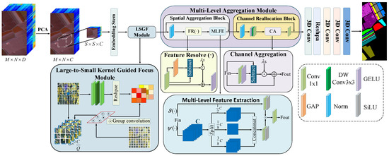
To fully utilize the spectral–spatial information of HSI and obtain rich multi-level features for more accurate and efficient classification, an LSGMA is designed. This network consists of an MLA and an LSGF module, and its overall architecture is illustrated in Figure 1. Initially, for a given input, HSI can be denoted as $X\in H\times W\times D$, where H and W are the height and width of spatial dimensions, and D represents the number of spectral bands. PCA is employed in this study to compress the spectral dimension of the HSI, thereby eliminating redundant information. After PCA dimensionality reduction, the spatial dimensions remain unchanged, while the spectral dimension is compressed from D to C. Meanwhile, essential spectral information is preserved throughout this process.

Figure 1. Overall structure diagram of the Large-to-Small Kernel Guided Multi-Level Aggregation network.

Subsequently, neighborhood patch extraction preprocessing is performed on the HSI after PCA processing. Specifically, an image patch is extracted around each pixel of the HSI, which serves as the input sample for the subsequent network. The label of the central pixel is assigned as the label for each image patch, denoted as $Z\in S\times S\times C$, with the width and height both transformed to S and the number of spectral bands changed to C. The image patches are first fed into an embedding stem to regulate the resolutions. Then the image patches are fed a second time into the LSGF. By combining LKS and SKD, the model’s ability to extract spatial neighborhood and central information is enhanced. After being processed by the LSGF, the features are passed into the MLA. After low-level and high-level interactive features are obtained, more discriminative mid-level interactive features, which are often neglected by previous networks, are further captured. Thus, feature representations with richer expressive power are acquired.

2.1. Large-to-Small Kernel Guided Focus Module

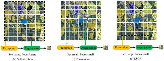
This paper proposes a novel strategy for perception and feature aggregation to achieve efficient feature interaction and fusion, as illustrated in Figure 2c. The method first captures comprehensive global context information through large-scale perception to model spatial relationships; subsequently, it employs small-scale feature aggregation operations to precisely fuse local, fine-grained features. Compared to the traditional methods shown in Figure 2a,b, this new strategy extracts complex local details more accurately while ensuring the full acquisition of global information, thereby effectively improving classification accuracy. Specifically, for feature $F_i$, the contextual perception region is $A_{\mathcal{P}}\left(F_i\right)$, and the aggregation region is $A_{\mathcal{A}}\left(F_i\right)$. Respectively, $A_{\mathcal{P}}\left(F_i\right)$ encompasses a larger spatial extent compared with $A_{\mathcal{A}}\left(F_i\right)$, the process can be formulated as follows:

$$Y_i=\mathcal{A}\left(\mathcal{P}\left(F_i,A_{\mathcal{P}}\left(F_i\right)\right),A_{\mathcal{A}}\left(F_i\right)\right).$$

(1)

where $\mathcal{P}$ represents perception and $\mathcal{A}$ represents aggregation.

Figure 2. Comparison of self-attention, convolution, and LS conv.

As can be observed from Equation (1), the context ranges employed in the perception and aggregation processes are different, namely $A_{\mathcal{P}}\left(F_i\right)$ and $A_{\mathcal{A}}\left(F_i\right)$, respectively, enabling the model to leverage multi-scale contextual information and simultaneously capture both global context information and intricate local feature details.

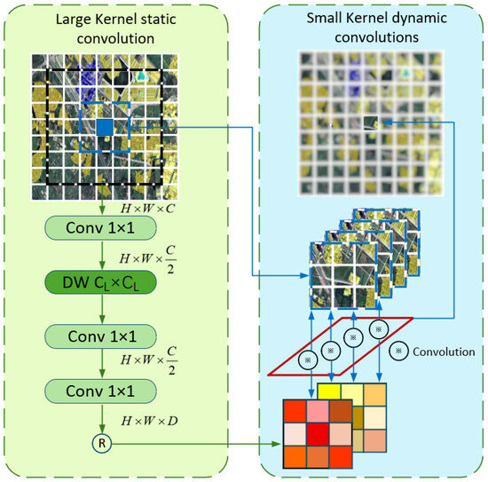
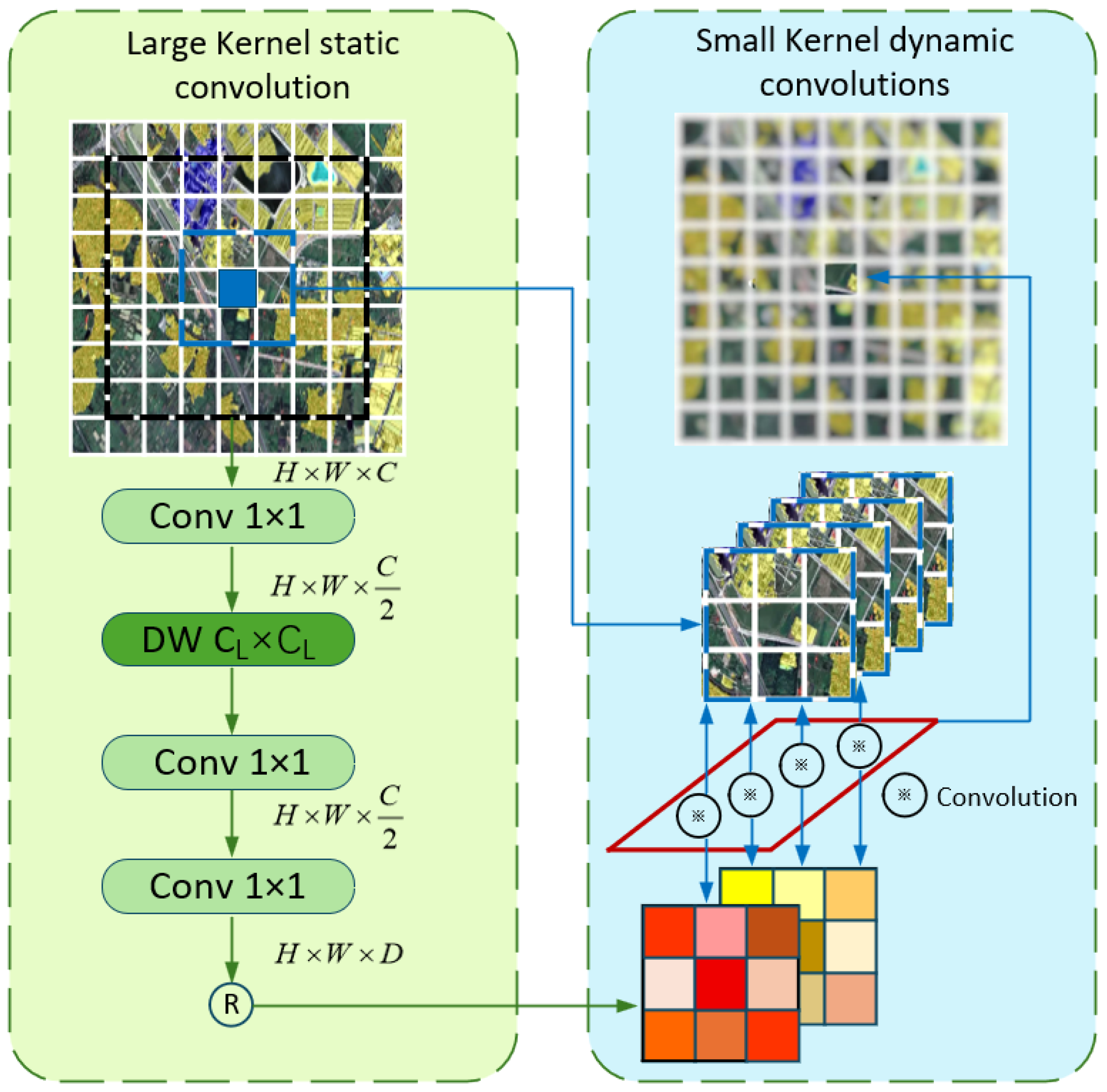
Based on the aforementioned design philosophy, this paper further proposes the LSGF convolution module. As illustrated in Figure 3, this module sequentially performs two stages of operations on each feature within the HSI: (1) large-kernel static convolution—utilizing large-sized static convolution kernels to expand the receptive field and capture richer contextual information; (2) small-kernel dynamic convolution—a form of small-kernel dynamic convolution incorporating a grouping mechanism, capable of adaptively aggregating complex local details.

Figure 3. Overall structure diagram of the LSGF.

2.1.1. Large-Kernel Static Convolution

Based on the input visual feature map $Z\in S\times S\times C$, the proposed LKS first performs channel dimensionality reduction through a pointwise convolution, reducing the number of channels to ${\displaystyle \frac{C}{2}}$. For the dimensionality-reduced feature $F_i$, a large-kernel depthwise convolution ($DW$) with a kernel size of $C_l\times C_l$ is then applied to capture large-field spatial neighborhood information of $A_{C_l}\left(F_i\right)$, where $A_{C_l}\left(F_i\right)$ denotes the surroundings of size $C_l\times C_l$ centered around $F_i$. The large-kernel $DW$ receptive field can be significantly expanded in an efficient manner, and the contextual perception capability can be enhanced. Subsequently, a PW is utilized to model spatial relationships among features, generating the context-adaptive weights $\mathrm{W}\in {\mathrm{R}}^{\mathrm{H}\times \mathrm{W}\times \mathrm{D}}$, which are applied in the subsequent aggregation process performed by the small-kernel dynamic convolution. The whole process can be formulated as follows:

$$W_i=PW\left(D{W}_{C_l\times C_l}\left(PW\left(A_{C_l}\left(F_i\right)\right)\right)\right.,$$

(2)

where $W_i\in {\mathrm{R}}^{\mathrm{D}}$ is the generated weights for $F_i$.

2.1.2. Small-Kernel Dynamic Convolution

A dynamic grouped convolution design is adopted in this module. For the generated feature maps $\mathrm{W}\in {\mathrm{R}}^{\mathrm{H}\times \mathrm{W}\times \mathrm{C}}$, a channel grouping strategy is adopted, dividing them into Q groups in total, with each group containing ${\displaystyle \frac{C}{Q}}$ channels, and the channels in the same group share the aggregation weights, to effectively reduce the model’s memory overhead and computational cost. Furthermore, the convolution kernel size for each group is adaptively adjusted based on different input data, which enhances the model’s adaptability and thereby strengthens its capability to handle complex data. For each $F_i$, we reshape its corresponding weights $W_i\in {\mathrm{R}}^{\mathrm{D}}$ generated by LKS to obtain $W_i^{*}\in R^{G\times C_s\times C_s}$, where $C_s\times C_s$ denotes the convolution kernel size of the small kernel. Subsequently, $W_i^{*}$ is utilized to guide the aggregation of highly related contextual information from $A_{C_s}\left(F_i\right)$, which $A_{C_s}\left(F_i\right)$ denotes the surroundings of size $C_s\times C_s$ centered at $F_i$. The c-th channel in $F_i$ is denoted as $F_{ic}$, which belongs to the q-th channel group. Finally, through a convolution operation between $A_{C_s}\left(F_i\right)$ and $W_{iq}^{*}\in R^{C_s\times C_s}$, the aggregated features are obtained and represented as $Y_{ic}$. In this manner, adaptive fine-grained features can be effectively represented, allowing the model to sensitively respond to dynamic and complex changes across different contexts. The whole process can be formulated as follows:

$$Y_{ic}=W_{iq}^{*}⊛{\mathrm{A}}_{{\mathrm{C}}_{\mathrm{s}}}\left(F_{ic}\right).$$

(3)

Rather than adopting a straightforward combination of large-kernel, small-kernel, and other dynamic convolutions, the proposed LSGF introduces an innovative approach. An LKS is utilized to achieve large-field visual perception, which in turn provides precise guidance for an SKD in performing adaptive feature fusion within highly relevant contextual information. As a result, the model’s capability to distinguish complex visual features is significantly enhanced.

2.2. Multi-Level Aggregation Module

As shown in Figure 1, after passing through the LSGF, the image flows into the MLA, which is composed of the Spatial Aggregation Block (SA) and Channel Reallocation Block (CR). MLA can further perform context aggregation and improve the accuracy of feature extraction.We integrate Feature Resolve (FR) and Multi-Level Feature Extraction (MLFE) into the Spatial Aggregation Block (SA) to force the aggregation of features encoded by previously neglected intermediate interactions, thereby enabling the model to achieve better performance on the HSI classification task. The Multi-Level Feature Aggregation also includes a Channel Reallocation Block (CR), which redistributes channels, forcing the model to encode previously ignored mid-level features while reducing channel redundancy.

2.2.1. Spatial Aggregation Block

DNNs with the incompatible composition of locality perception and context aggregation can be implicitly prone to extreme-level game-theoretic interaction strengths while suppressing the more robust and expressive mid-level ones. Currently, the primary obstacle lies in compelling the network to encode the originally ignored expressive interactions and informative features. To address this, we propose the SA, which consists of two cascaded components, designed to learn representations of multi-level interactions within an integrated framework. This can be formulated as follows:

$$\mathrm{Z}=\mathrm{FR}(·)+MlFE\left(\mathrm{FR}\right(Norm\left(\mathrm{F}\right)\left)\right),$$

(4)

where $FR(·)$ refers to a Feature Resolve module; $MLFE(·)$ refers to a Multi-level feature extraction module, which is composed of the context feature extraction branch $\vartheta (·)$ and the multi-level aggregation branch $\psi (·)$; and Z represents the downsampled feature.

Context Extraction

A purely ConvNet structure is established, which focuses on extracting multi-level features with both static and adaptive locality perceptions. There are two complementary counterparts, $\mathrm{Conv}1\times 1(·)$ and $GAP(·)$ layers, which are designed to instantiate fine-grained local textures and complex global shapes respectively. To prevent the network from neglecting mid-level interactions, $FR(·)$ is designed to adaptively exclude the neglected interactions, which are defined as follows:

$$Y={\mathrm{Conv}}_{1\times 1}1\left(F\right),$$

(5)

$$\mathrm{Z}=\mathrm{GELU}\left(\mathrm{Y}+{\lambda }_{\mathrm{s}}\odot (\mathrm{Y}-\mathrm{GAP}\left(\mathrm{Y}\right))\right),$$

(6)

The scaling factor ${\lambda }_s\in R^{C\times 1}$ is initialized as zero. The $FR(·)$ effectively enhances the spatial diversities of features by reweighting the complementary interaction component $\mathrm{Y}-\mathrm{GAP}\left(\mathrm{Y}\right)$. Furthermore, a depth-wise convolution (DWConv) is introduced into the contextual branch of the $MLFE(·)$ to encode multi-level features. Different from the traditional approaches that combine DWConv with self-attention to model global and local interactions, we innovatively deploy three different parallel DWConv layers with a dilation ratio $d\in \{1,2,3\}$ to comprehensively capture low, mid, and high-level interactions. Given the input feature $F\in R^{C\times HW}$, it is first processed by a DWConv with a $5\times 5$ kernel and a dilation ratio of 1 to extract low-level features. The output is then split along the channel dimension into: ${\mathrm{F}}_l\in {\mathrm{R}}^{{\mathrm{C}}_l\times \mathrm{HW}}$, ${\mathrm{F}}_m\in {\mathrm{R}}^{{\mathrm{C}}_m\times \mathrm{HW}}$, ${\mathrm{F}}_h\in {\mathrm{R}}^{{\mathrm{C}}_h\times \mathrm{HW}}$, where $C=C_l+C_m+C_h$; among them, $C_l$ serves as the identical mapping and is directly output, while $C_m$ and $C_h$ are respectively processed by DWConv with kernel sizes of $5\times 5$ (dilation rate $d=2$) and $5\times 5$ (dilation rate $d=3$), to respectively capture mid- and high-level features. Finally, the outputs of the three branches are concatenated to form the multi-level contexts $Y_C=Concat\left(Y_{l,1:C_l},Y_m,Y_h\right)$.

Multi-Level Feature Aggregation

To adaptively aggregate the multi-order features extracted from context feature extraction branches, we employ SiLU for activation in the multi-level aggregation branch. This function not only exhibits the gating effect as a sigmoid but also possesses a stable training property. It takes the output $FR(·)$ as input, and is formulated as follows:

$$Z=\underset{\psi }{\underbrace{SiLU\left({Conv}_{1\times 1}\left(F\right)\right)}}\odot \underset{\vartheta }{\underbrace{SiLU\left({Conv}_{1\times 1}\left(Y_C\right)\right)}}.$$

(7)

With the SA blocks, LSGMA can extract more mid-level interactions that were overlooked by previous networks, enabling the model to capture more comprehensive and abundant multi-level features.

2.2.2. Channel Reallocation Block

Drawing inspiration from the $FR(·)$ concept mentioned above, we designed a lightweight Channel Aggregation $CA(·)$ to adaptively reallocate channel-wise features in high-dimensional hidden spaces. Subsequently, we further extend it into a CR, which can be formulated as follows:

$$\begin{array}{c}Y=GELU\left({DW}_{3\times 3}\left({Conv}_{1\times 1}(Norm\left(X\right))\right)\right),\hfill \\ Z={Conv}_{1\times 1}(CA\left(Y\right))+X.\hfill \end{array}$$

(8)

The specific implementation of $CA(·)$ can be decomposed into two steps. First, a channel-reducing projection $W_r:{\mathrm{R}}^{\mathrm{C}\times \mathrm{HW}}\to {\mathrm{R}}^{1\times \mathrm{HW}}$. Second, the GELU activation function is employed. This process aims to aggregate channel-wise information and achieve its adaptive reallocation.

$$CA\left(\mathrm{X}\right)=\mathrm{X}+{\lambda }_{\mathrm{s}}\odot \left(\mathrm{F}-GELU\left({\mathrm{FW}}_{\mathrm{r}}\right)\right),$$

(9)

Among them, the channel-wise scaling factor ${\lambda }_{\mathrm{s}}$ is initialized to zero. It leverages the complementary interaction $\left(\mathrm{F}-GELU\left({\mathrm{FW}}_{\mathrm{r}}\right)\right)$ to achieve the reallocation of channel-wise features. In this way, $CA(·)$ enhances the previously overlooked game-theoretic interactions.

3. Experiments and Results

In this section, we introduce the four datasets used in the experiments as well as the settings of various model parameters, and focus on discussing the comparison results of the proposed LSGMA against various methods on the datasets. Four public datasets are employed, namely the QUH-Pingan datasets (Pingan) [34], the Salinas datasets (Sa) [35], the QUH-Qingyun datasets (Qingyun) [34], and the WHU-Hi-Longkou (WHU) [36] datasets. The four datasets mentioned above are large in volume and densely labeled. An excessively high training ratio could lead to “precision saturation” in deep learning models, causing all comparison methods to achieve high classification accuracy on these datasets, thus failing to effectively differentiate the performance of different algorithms. Therefore, we set the training ratios for the four datasets to 3%, 0.5%, 1%, and 0.5%, with three datasets being drone-captured images. Smaller training ratios better align with the practical application scenario of “low labeling cost, wide-area prediction” in drone inspections. Simultaneously, we adopted a stratified sampling classification method, sampling independently by category to ensure a consistent proportion of training samples for each land cover type. This prevents excessive samples from large categories from crowding out training resources for rarer minor categories, ensuring equal training and evaluation conditions for each category, and resulting in objective and fair statistical results for classification metrics.

3.1. Datasets Description

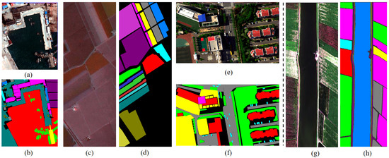
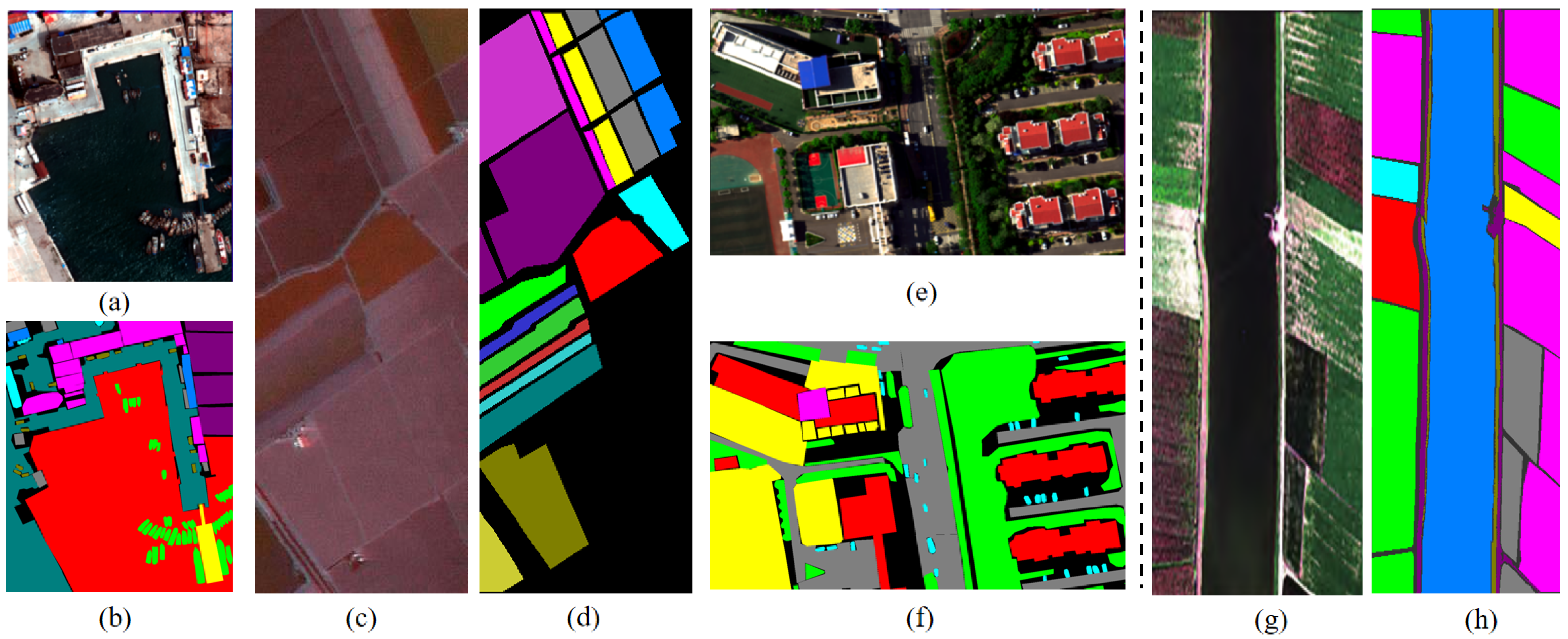
QUH-Pingan Datasets: The QUH-Pingan dataset was acquired from 10:43 to 11:28 on 19 May 2021, in Huangdao Pingan Passenger Ship Terminal, Qingdao, China. The UAV flew at an altitude of 200 m, and the spatial resolution of the UAV-borne hyperspectral imagery is about 0.10 m. This dataset has a spatial size of 1230 × 1000 pixels and 176 bands with a wavelength range of 400–1000 nm. This dataset has 10 land cover classes, but there are large differences in size, including seawater and roads at large scales; trees, floating piers, brick houses, and steel houses at medium scales; and ships and cars at small scales, which are the most difficult to identify. In addition, this dataset is one of the few that contains data from the marina scene among previous datasets. The training set was configured to 3% of the total data, and the specific number of training samples is detailed in Table 1. The false-color image and ground-truth map of QUH-Pingan are shown in Figure 4.

Table 1. Category and quantity on four datasets.

QUH-Pingan [34]				Salinas [35]				QUH-Qingyun [34]				WHU-Hi-Longkou [36]
Class	Category	Train	Test	Class	Category	Train	Test	Class	Category	Train	Test	Class	Category	Train	Test
1	Ship	1468	47,467	1	Alfalfa	5	41	1	Trees	2781	275,369	1	Corn	172	34,339
2	Seawater	17,343	560,770	2	Corn-notill	143	1285	2	Concrete building	1795	177,717	2	Cotton	42	8332
3	Trees	250	8095	3	Corn-mintill	83	747	3	Car	138	13,645	3	sesame	15	3016
4	Concrete structure building	2669	86,304	4	Corn	24	213	4	Tronhide building	98	9669	4	Broad-leaf-soybean	316	62,896
5	Floating pier	623	20,136	5	Grass-pasture	48	435	5	Plastic playground	2177	215,558	5	Narrow-leaf-soybeans	21	4130
6	Brick houses	423	13,663	6	Grass-tress	73	657	6	Asphal road	2559	253,387	6	Rice	59	11,795
7	Steel houses	420	13,571	7	Grass-pasture-mowed	3	25					7	Water	335	66,721
8	Wharf construction land	2493	80,620	8	Hay-windrowed	48	430					8	Roads and houses	36	7088
9	Car	243	7865	9	Oats	2	18					9	Mixed-weed	26	5203
10	Road	8296	268,218	10	Soyben-notill	97	875
				11	Soybean-mintill	245	2210
				12	Soybean-clean	59	534
				13	Wheat	20	185
				14	Woods	126	1139
				15	Building-grass-tress-drives	39	347
				16	Stone-steel-towers	9	84
Total		34,228	1,106,709	Total		1024	9225	Total		9548	945,345	Total		1022	203,520

Figure 4. (a) False color image of QUH-Pingan. (b) Ground-truth map of QUH-Pingan. (c) False color image of Salinas. (d) Ground-truth map of Salinas. (e) False color image of QUH-Qingyun. (f) Ground-truth mao of QUH-Qingyun. (g) False color image of WHU-Hi-Longkou. (h) Ground-truth WHU-Hi-Longkou.

Salinas Dataset: This dataset was acquired by the AVIRIS sensor in 1998 over the Salinas Valley region of California, USA. The size of the imagery is 512 × 217 pixels, totaling 111,000 pixels with a spatial resolution of 3.7 m. It comprises 224 contiguous spectral bands; after removing 20 water absorption bands, 204 spectral bands remain for classification tasks. The labeled pixels total 54,129, divided into 16 classes. The training set was configured to 0.5% of the total data, and the specific number of training samples is detailed in Table 1. The false-color image and ground-truth map of Salinas are shown in Figure 4.

QUH-Qingyun Dataset: The QUH-Qingyun dataset was acquired in the vicinity of Qingyun Road Primary School and the surrounding residential area in Qingdao City, Shandong Province, China. The UAV flew at an altitude of 300 m, and the size of the imagery is 880 × 1360 pixels. There are 270 bands from 400 to 1000 nm, and the spatial resolution is about 0.15 m. This dataset has a relatively limited number of land cover categories, with only 6 types. However, this dataset has areas obscured by building shadows, including classes such as trees, cars, and asphalt roads. The interference of shadows can significantly reduce the accuracy of identification and can be used to assess the robustness of the classification methods. The training set was configured to 1% of the total data, and the specific numbers of training samples are listed in Table 1. The false-color image and ground-truth map of QUH-Qingyun are shown in Figure 4.

WHU-Hi-Longkou Dataset: This dataset was provided by the RSIDEA Team of Wuhan University. Captured over Longkou Town, Hubei Province, China, and acquired using a Headwall Nano-Hyperspec imaging sensor mounted on the DJI Matrice 600 Pro (The manufacturer of the DJI Matrice 600 Pro is DJI, and its headquarters is located in Shenzhen, Guangdong Province, China.). Unmanned Aerial Vehicle (UAV) platform. The image size is 550 × 400 pixels, resulting in 220,000 total pixels, with the spatial resolution of the UAV-borne hyperspectral imagery being about 0.463 m. The dataset comprises 270 contiguous spectral bands. The labeled pixels are divided into 9 classes. The training set was configured to 0.5% of the total data, and the specific numbers of training samples are detailed in Table 1. The false-color image and ground-truth map of WHU-Hi-Longkou are shown in Figure 4.

3.2. Experiment Setting and Assessment Criteria

All experiments were conducted by PyTorch 3.12.9 on a computer equipped with a GeForce RTX 4060 graphics processing unit (GPU), an Intel(R) Core(TM) i9-14900HX CPU, and 32 GB RAM. The cross-entropy loss function was used to calculate the associated loss, and the Adam optimizer was used for network optimization with the initial learning rate set to $1\times {10}^{-2}$. The network was trained for 200 epochs with a batch size of 16.

We adopt three widely used criteria to evaluate the performance of HSIC: Overall Accuracy (OA), Kappa coefficient (kappa), and Average Accuracy (AA). The OA represents the proportion of correctly classified samples among the total test samples; kappa reflects the consistency between the classification results and the ground truth, and AA is the mean of the classification accuracy of all classes.

3.3. Parameter Analysis

This part primarily analyzes the impact of various parameters in the network on classification results. The model’s classification performance depends not only on its structural design but also on the setting of various parameters. Specifically, this part mainly discusses the influence of the datasets’ patch size, PCA dimensionality and the sizes of large and small kernels in the LSGF on classification accuracy. All experiments were conducted across the aforementioned four datasets, employing a control variable method to analyze the influence of parameters, thereby ensuring the reliability of the results.

3.3.1. Influence of the Patch Size

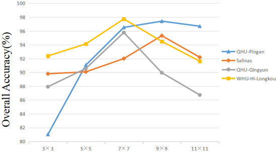
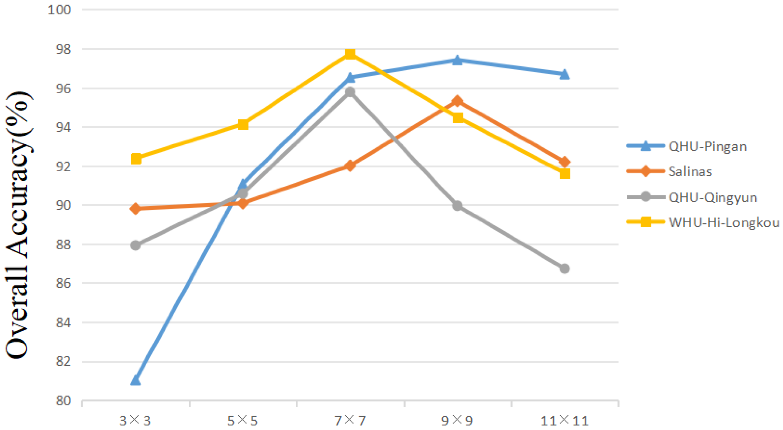
In HSIC tasks, image patches are typically used as network inputs to capture spatial information for assisting the decision-making process. However, the size of the input image patches is closely related to the scope and quality of the spatial information that can be obtained. To this end, we investigate the impact of different patch sizes on HSIC performance. Thus, we keep other factors, set the patch sizes of four datasets to $3\times 3$, $5\times 5$, $7\times 7$, $9\times 9$, and $11\times 11$, and compared the classification accuracy of the LSGMA under different patch sizes. Figure 5 shows the influence of different spatial sizes on the OA.

Figure 5. Classification results of different patch sizes.

As can be observed from the Figure 5, the OA values of the QUH-Qingyun and Salinas datasets reach their maximum when the patch size increases to $9\times 9$; beyond this size, the OA values begin to decline. For the QUH-Pingan and WHU-Hi-Longkou datasets, the OA values peak when the patch size reaches $7\times 7$. This is mainly because the objects captured in the QUH-Pingan and Salinas datasets are respectively the docks and agricultural areas. In these regions, land cover categories usually have relatively regular distributions, but there are significant differences in size among the various categories. In contrast, the QUH-Qingyun and WHU datasets have smaller capture ranges. The QUH-Qingyun dataset mainly focuses on the Qingyun Road University and its surrounding urban areas, featuring complex and interwoven category distributions. Meanwhile, although the WHU dataset is also an agricultural area, its land cover categories are interlaced. Therefore, we selected the block size corresponding to the maximum OA value for each dataset, that is, $9\times 9$ for the QUH-Pingan and Salinas datasets, and $7\times 7$ for the QUH-Qingyun and WHU-Hi-Longkou datasets.

3.3.2. Influence of the PCA Dimension

While the multiple bands of HSI provide rich information, too many bands also create information redundancy, increasing the computational cost of subsequent processing tasks. Furthermore, when the number of training samples is limited, the overall classification accuracy of HSI tends to decrease with increasing feature dimensionality, a phenomenon known as the curse of dimensionality. Therefore, it is necessary to reduce information redundancy by decreasing the spectral dimensionality of HSI. PCA is a commonly used dimensionality reduction method, whose core idea is to extract key features by calculating the similarity between different data. However, different PCA dimensions can affect the model’s classification results. Therefore, we investigated the impact of different PCA dimensions on the HSI classification task.

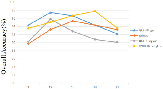
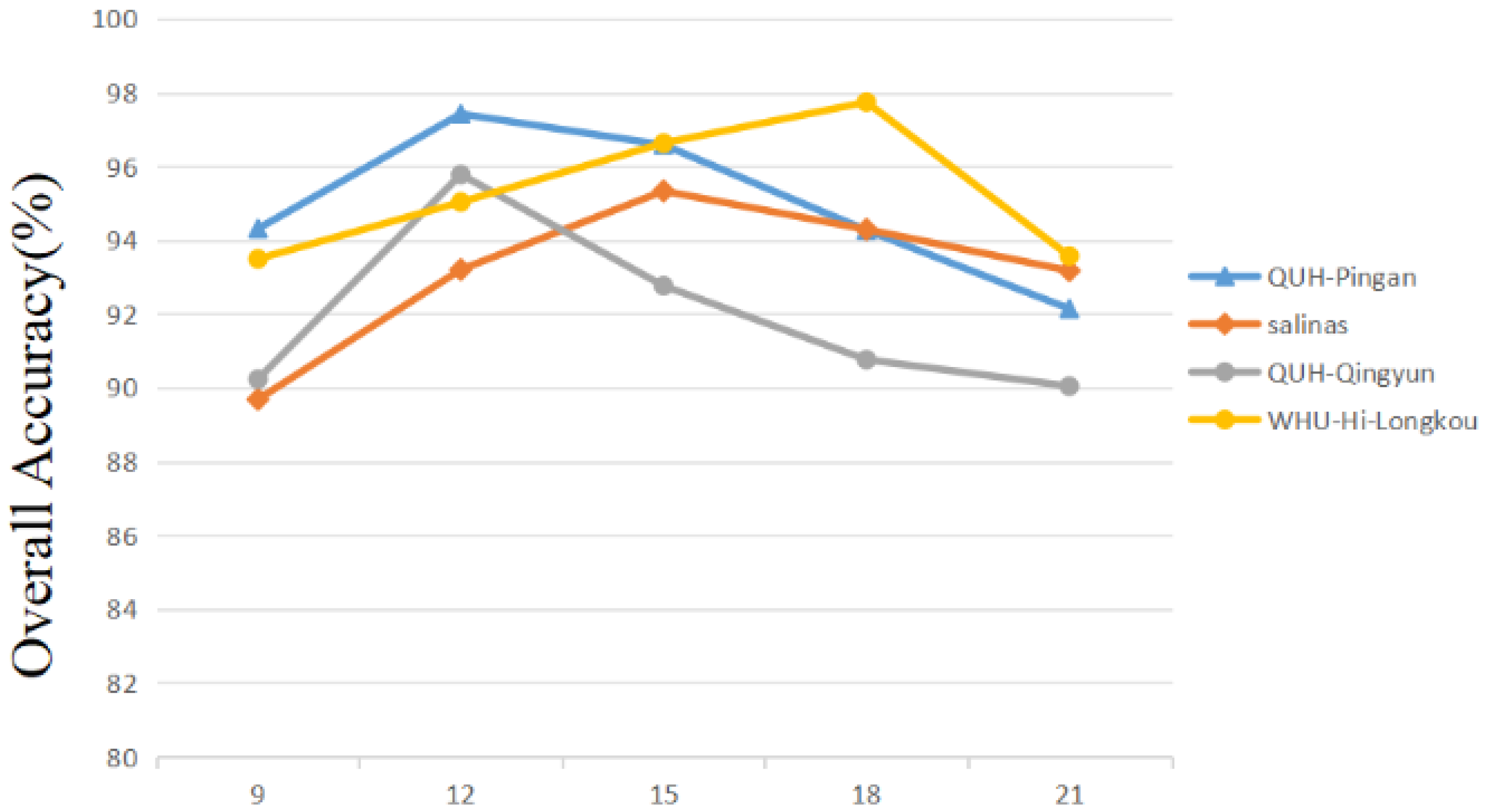
As shown in Figure 6, the appropriate PCA dimension varies for each dataset, determined by its characteristics. Excessively high PCA dimensionality usually leads to the retention of too much information, resulting in redundancy even after dimensionality reduction; conversely, excessively low PCA dimensionality may lead to the loss of useful information, ultimately resulting in a decrease in classification accuracy. Based on Figure 6, this paper sets the PCA dimension to 12 for the QUH-Pingan and QUH-Qingyun datasets, 15 for the Salinas dataset, and 18 for the WHU-Hi-Longkou dataset.

Figure 6. Classification results on different of PCA dimension on different datasets.

3.3.3. Influence of the Large and Small Kernel Sizes

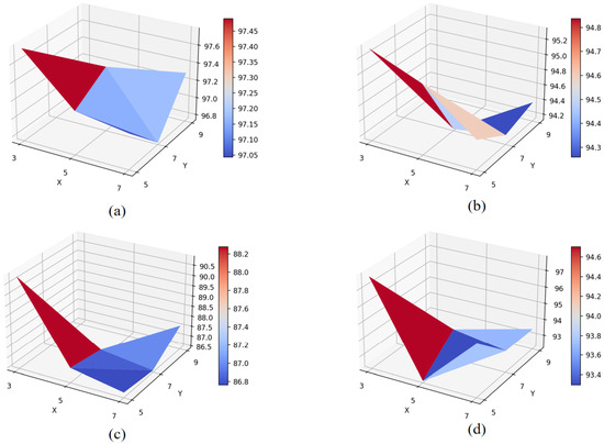
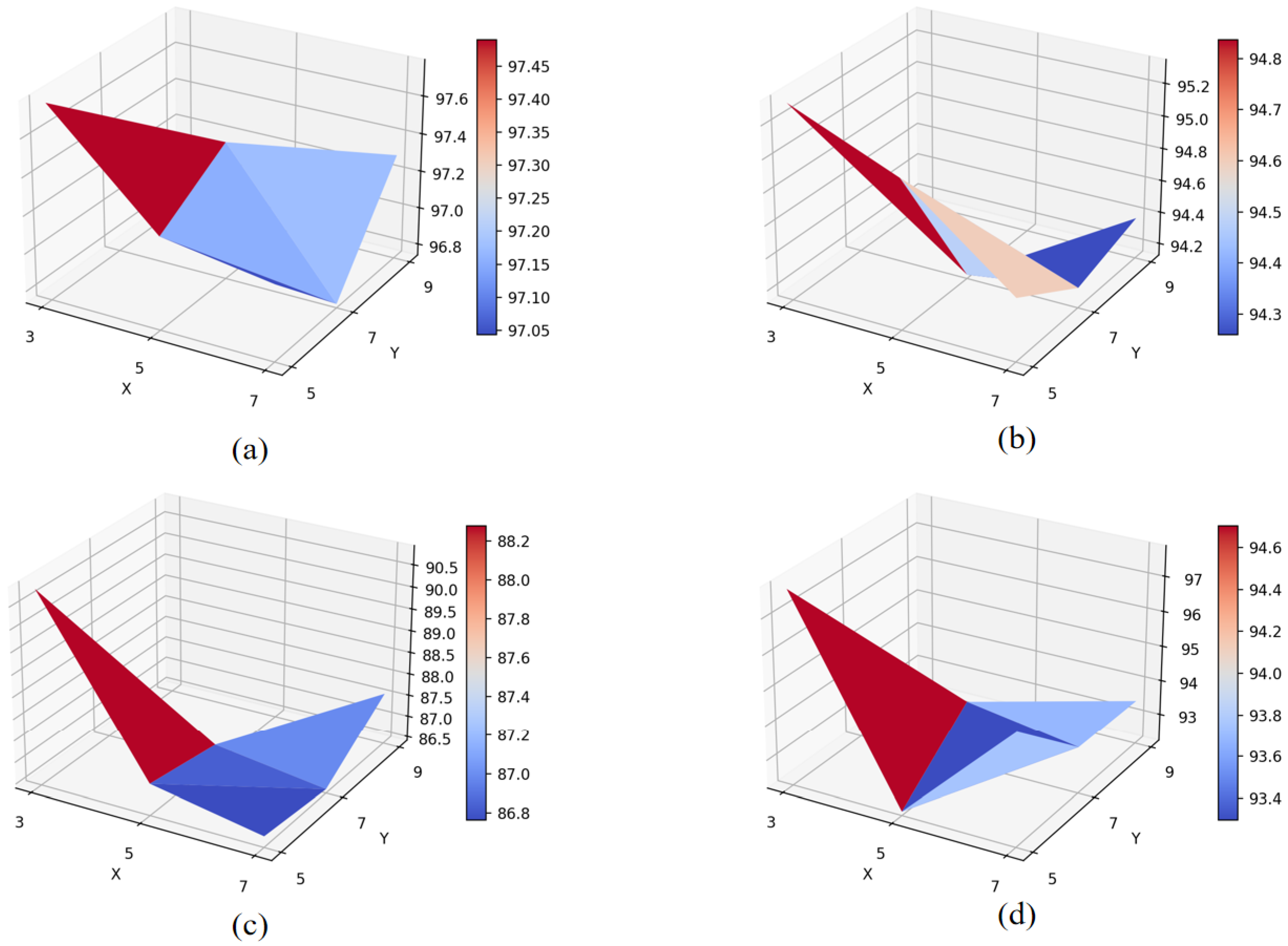
In the LSGF module, the large-kernel (Y) size determines the scope of contextual information that the model can capture, while the small-kernel (X) size determines the scope of feature aggregation. Therefore, their interaction jointly influences the classification performance of the model. In order to set more reasonable parameters on LSGMA, we conducted experiments to determine the optimal combination of large and small kernel sizes. We set the large kernel sizes to 5, 7, and 9, and the small kernel sizes to 3, 5, and 7, evaluating all pairwise combinations on four datasets. Figure 7 illustrates the classification outcomes of different kernel size combinations on the four datasets.

Figure 7. Classification results on combinations of large and small kernel sizes on different datasets. (Figure display) (a) QUH-Pingan. (b) Salinas. (c) QUH-Qingyun. (d) WHU-Hi-Longkou.

As shown in Figure 7 and Table 2, when the small kernel size remains constant, the model can acquire more spatial contextual features as the large kernel size increases, leading to a corresponding increase in the amount of information to be processed. However, information redundancy also intensifies, creating additional difficulties for subsequent kernel processing. Therefore, the overall accuracy (OA) decreases with increasing kernel size on all four datasets. This result indicates that the model requires more efficient information, not more information. When the large kernel size remains constant, the spatial contextual information acquired by the model is fixed. In this case, increasing the small kernel size means expanding the focusing range, causing the model to fail to accurately focus on local details, resulting in insufficient feature extraction. Therefore, the overall accuracy (OA) decreases with increasing small kernel size on all four datasets. Experimental results show that the OA values are highest on all four datasets when the large kernel size is 5, and the small kernel size is 3, corresponding to the optimal spatial context perception range and feature focusing range. Therefore, for these four datasets, we set the large kernel size to 5 and the small kernel size to 3.

Table 2. Classification results on combinations of large and small kernel sizes on different datasets. (a) QUH-Pingan. (b) Salinas. (c) QUH-Qingyun. (d) WHU-Hi-Longkou.

	(a) Large Kernel	5	7	9		(b) Large Kernel	5	7	9
(a) Small Kernel					(b) Small Kernel
3		97.43	97.23	97.14	3		95.32	95.04	94.51
5		\	97.13	96.59	5		\	94.15	94.25
7		\	\	96.30	7		\	\	94.22
	(c) Large Kernel	5	7	9		(d) Large Kernel	5	7	9
(c) Small Kernel					(d) Small Kernel
3		95.78	92.43	91.66	3		97.75	92.32	95.40
5		\	91.86	91.50	5		\	94.04	95.37
7		\	\	91.37	7		\	\	93.48

3.4. Analysis of Classification Results

To evaluate the performance of the LSGMA for HSIC, it was compared with several state-of-the-art classification models. Specifically, our model was primarily compared against the following approaches: (1) Spectral Spatial Feature Tokenization Transformer (SSFTT) [37]; (2) SpectralFormer [38]; (3) Lightweight Hybrid Convolutional Neural Network (Lite-HCNet) [39]; (4) Groupwise Separable Convolutional ViT (GSC-ViT) [40]; (5) Lightweight Spectral–Spatial Attention Network (LSSAN) [41]; (6) Covariance Attention and Cross-layer Fusion Transformer Network (CACFTNet) [42]; (7) Multiscale Densely Connected Attention Network (MSDAN) [43]; (8) SimPoolFormer [44]; and (9) Dynamic Graph Enhancement and Hierarchical Feature Fusion model (DEHF) [45].

3.4.1. Results of QUH-Pingan

The classification results of different methods on the QUH-Pingan datasets are listed in Table 3 (the bold font in the table indicates the best performance among all the methods). The visual maps of the various methods are shown in Figure 8.

Table 3. Accuracy evaluation results of the QUH-Pingan Dataset.

Class	SSFTT	SpectralFormer	Lite-HCNet	Gsc-Vit	LSSAN	CACFTNet	MSDAN	SimPoolFormer	DEHF	LSGMA
1	78.67 ± 9.86	69.69 ± 14.62	76.39 ± 1.99	84.79 ± 0.59	83.56 ± 13.84	78.57 ± 8.80	75.43 ± 7.83	87.51 ± 10.42	78.62 ± 7.21	86.94 ± 7.98
2	98.87 ± 0.67	98.34 ± 3.38	98.61 ± 0.40	98.60 ± 2.11	98.95 ± 1.44	98.71 ± 0.55	98.80 ± 1.63	98.71 ± 2.00	98.65 ± 1.78	99.15 ± 1.00
3	62.03 ± 1.6	66.90 ± 1.67	79.57 ± 1.05	87.68 ± 3.02	80.79 ± 5.42	74.66 ± 1.75	77.63 ± 1.60	53.35 ± 2.93	52.76 ± 2.41	88.22 ± 0.53
4	74.85 ± 5.79	76.47 ± 5.89	73.37 ± 4.22	88.59 ± 1.85	81.84 ± 13.65	86.62 ± 3.32	82.73 ± 3.92	66.63 ± 11.05	90.07 ± 6.43	95.87 ± 1.12
5	16.08 ± 0.38	70.32 ± 1.78	56.05 ± 0.77	68.99 ± 1.11	34.15 ± 1.67	62.20 ± 0.89	44.83 ± 0.85	45.39 ± 2.30	69.69 ± 0.83	94.35 ± 0.91
6	1.81 ± 0.42	70.13 ± 0.63	68.93 ± 0.44	88.23 ± 1.54	68.61 ± 1.13	70.00 ± 0.68	46.30 ± 0.98	69.95 ± 0.91	88.61 ± 1.31	95.41 ± 0.54
7	73.01 ± 8.22	82.78 ± 8.38	78.94 ± 1.60	85.79 ± 0.57	72.77 ± 15.28	86.94 ± 18.73	79.96 ± 0.00	89.02 ± 9.58	92.87 ± 5.61	92.83 ± 0.63
8	80.78 ± 13.37	81.47 ± 0.55	85.54 ± 1.26	88.68 ± 0.34	76.42 ± 0.41	86.85 ± 0.35	81.77 ± 0.61	81.58 ± 0.44	75.15 ± 1.92	94.74 ± 0.10
9	1.36 ± 16.73	12.02 ± 13.87	35.94 ± 6.52	35.93 ± 9.62	3.70 ± 19.49	22.64 ± 18.57	6.47 ± 29.29	45.27 ± 6.52	51.42 ± 8.49	77.46 ± 8.43
10	94.05 ± 0.49	97.26 ± 3.00	94.48 ± 1.06	97.22 ± 1.47	95.72 ± 1.90	96.33 ± 1.21	97.14 ± 1.46	93.04 ± 2.18	95.12 ± 2.91	98.39 ± 1.11
OA%	89.65 ± 0.19	92.02 ± 0.63	91.77 ± 0.14	94.82 ± 0.63	91.84 ± 1.24	93.58 ± 0.49	92.23 ± 0.67	90.95 ± 1.49	93.16 ± 1.16	97.42 ± 0.21
AA%	58.04 ± 1.25	72.54 ± 1.54	74.78 ± 0.54	82.45 ± 0.95	69.65 ± 2.15	76.35 ± 1.90	69.11 ± 1.12	73.04 ± 1.96	79.30 ± 1.83	92.34 ± 0.65
Kappa%	84.46 ± 0.22	88.06 ± 0.71	87.66 ± 0.16	92.28 ± 0.71	87.80 ± 1.42	90.42 ± 0.56	88.33 ± 0.76	86.47 ± 1.71	89.80 ± 0.67	96.15 ± 0.23

Figure 8. Ground-truth and classification maps of different methods on QUH-Pingan. (a) Ground-truth map. (b) SSFTT. (c) SpectralFormer. (d) Lite-HCNet. (e) GSC-ViT. (f) LSSAN. (g) CACFTNet. (h) MSDAN. (i) Sim Pool Former. (j) LSGMA.

As shown in Table 3, in the QUH-Pingan dataset, the proposed LSGMA network achieves the best classification performance in terms of three evaluation metrics: overall accuracy (OA), average accuracy (AA), and the Kappa coefficient. Among the eight mainstream methods, except for CACFTNet and Gsc-Vit, the OA improvement over the remaining six methods is more than 5%. Specifically, compared with SSFTT, the OA improvement reaches 7.77%. In addition, LSGMA still outperforms CACFTnet and Gsc-ViT, achieving OA improvements of 3.84% and 2.95%, respectively. Moreover, LSGMA attains the highest accuracy on nine out of ten classes in this dataset (seawater, trees, concrete structure building, floating pier, brick houses, Wharf construction land, car, road), demonstrating its superiority in recognizing datasets containing classes with large variations in object size.

Figure 8 shows the visual maps of various methods on the QUH-Pingan dataset. For clarity, the ground-truth map is first displayed in Figure 8a. Due to the significant class size imbalance in the QUH-Pingan dataset, it is clearly observed that the compared methods, when handling such imbalanced categories, tend to misclassify adjacent classes with large size disparities. Specifically, small-sized classes are often misidentified as part of large-sized classes, or small classes intrude into the regions of large classes. For instance, SSFTT and LSSAN misclassify Class 5 (floating pier) as Class 1 (ship). Most methods erroneously recognize Class 9 (car) as part of Class 10 (road), and Class 6 (brick houses) as part of Class 7 (steel houses). In contrast, LSGMA is able to accurately identify small-sized classes of targets when recognizing objects with significant size differences. For example, it does not misclassify small-sized classes such as trees (category 3) and cars (category 9) as large-sized, neighboring classes. This advantage can be attributed to LSGMA’s ability to simultaneously capture both spatial neighborhood information and central information, thereby enabling more effective classification on datasets containing classes with pronounced size differences.

3.4.2. Result of Salinas

The classification results of different methods on the Salinas datasets are listed in Table 4 (the bold font in the table indicates the best performance among all the methods), The visual maps of the various methods are shown in Figure 9.

Table 4. Accuracy evaluation results of the Salinas dataset.

Class	SSFTT	SpectralFormer	Lite-HCNet	Gsc-Vit	LSSAN	CACFTNet	MSDAN	SimPoolFormer	DEHF	LSGMA
1	99.83 ± 0.25	98.12 ± 1.15	99.89 ± 0.15	99.94 ± 0.11	97.63 ± 2.17	96.62 ± 3.44	99.25 ± 1.68	99.74 ± 0.35	95.32 ± 3.14	99.75 ± 0.38
2	99.96 ± 0.07	99.94 ± 0.07	99.99 ± 0.02	100.00 ± 0.00	99.80 ± 0.25	98.75 ± 1.30	99.81 ± 0.27	99.68 ± 0.51	99.95 ± 0.53	99.98 ± 0.02
3	99.51 ± 0.24	98.00 ± 1.48	99.83 ± 0.09	99.27 ± 0.66	94.80 ± 3.97	94.88 ± 1.76	98.74 ± 0.64	97.01 ± 2.34	99.44 ± 1.64	99.64 ± 0.50
4	94.78 ± 3.22	90.84 ± 6.68	91.62 ± 4.98	91.58 ± 7.25	86.91 ± 9.84	74.71 ± 11.35	82.81 ± 12.24	95.25 ± 3.07	89.64 ± 2.72	95.74 ± 3.43
5	97.48 ± 0.26	98.51 ± 0.74	97.70 ± 1.28	96.49 ± 1.45	97.25 ± 1.01	95.92 ± 1.75	91.23 ± 6.97	93.87 ± 1.55	99.32 ± 1.19	97.84 ± 1.11
6	100.00 ± 0.00	99.96 ± 0.05	99.98 ± 0.02	99.93 ± 0.10	99.90 ± 0.12	96.72 ± 2.51	99.05 ± 0.98	99.83 ± 0.30	99.95 ± 0.28	99.75 ± 0.27
7	99.42 ± 0.65	99.47 ± 0.14	98.91 ± 0.86	99.71 ± 0.58	96.94 ± 1.80	94.17 ± 5.83	98.45 ± 0.74	98.59 ± 0.87	99.86 ± 0.61	98.80 ± 0.61
8	89.10 ± 0.98	84.36 ± 3.33	86.62 ± 2.20	86.88 ± 2.78	83.65 ± 2.88	83.44 ± 3.96	85.69 ± 3.32	83.76 ± 3.36	85.94 ± 2.39	88.26 ± 1.63
9	100.00 ± 0.00	99.79 ± 0.45	100.00 ± 0.00	99.98 ± 0.03	99.84 ± 0.18	99.71 ± 0.33	99.79 ± 0.39	100.00 ± 0.00	100.00 ± 0.00	100.00 ± 0.00
10	96.60 ± 0.63	92.98 ± 1.41	96.93 ± 0.55	96.46 ± 0.81	93.43 ± 1.06	91.62 ± 5.00	95.45 ± 2.90	95.35 ± 0.96	92.54 ± 1.95	97.70 ± 0.73
11	91.6 ± 1.69	93.87 ± 3.06	95.40 ± 3.21	97.71 ± 1.87	87.26 ± 6.65	75.65 ± 8.61	86.35 ± 7.04	96.01 ± 2.73	88.36 ± 2.14	98.46 ± 1.19
12	99.43 ± 0.99	99.43 ± 0.47	99.99 ± 0.02	98.86 ± 0.95	96.06 ± 3.40	96.09 ± 3.78	96.03 ± 2.19	98.63 ± 1.29	95.34 ± 1.94	99.20 ± 0.97
13	94.36 ± 4.97	90.43 ± 8.28	77.91 ± 16.78	70.83 ± 29.82	94.80 ± 3.82	89.51 ± 9.79	65.55 ± 36.41	74.16 ± 40.42	96.03 ± 10.28	95.66 ± 2.62
14	91.29 ± 4.76	89.1 ± 12.73	92.50 ± 2.30	90.67 ± 4.80	89.39 ± 3.29	91.31 ± 4.13	90.84 ± 5.50	93.80 ± 4.65	87.16 ± 3.67	98.03 ± 1.55
15	80.14 ± 1.47	77.67 ± 3.20	86.2 ± 1.04	90.26 ± 2.91	70.90 ± 4.42	82.53 ± 2.93	77.48 ± 7.12	78.06 ± 4.81	79.10 ± 5.76	88.42 ± 3.53
16	97.04 ± 1.76	97.98 ± 0.46	99.06 ± 0.42	98.27 ± 0.58	95.16 ± 5.17	81.63 ± 20.50	96.61 ± 3.03	92.52 ± 6.36	95.70 ± 4.92	99.29 ± 0.35
OA%	93.98 ± 0.43	92.24 ± 0.87	94.12 ± 0.29	94.48 ± 0.53	90.45 ± 1.27	90.21 ± 1.35	91.27 ± 0.21	91.78 ± 0.92	92.44 ± 0.72	95.33 ± 0.1
AA%	95.65 ± 0.83	94.42 ± 1.69	95.16 ± 0.67	94.80 ± 1.82	92.73 ± 1.65	90.20 ± 1.46	91.44 ± 2.18	93.52 ± 2.85	93.98 ± 2.41	97.28 ± 0.36
Kappa%	93.29 ± 0.48	91.36 ± 0.97	93.45 ± 0.31	93.86 ± 0.59	89.36 ± 1.42	89.10 ± 1.49	90.28 ± 0.23	90.85 ± 1.02	91.58 ± 0.84	94.80 ± 0.12

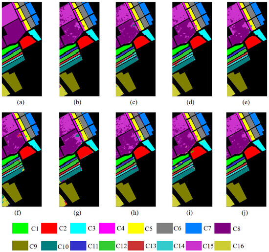
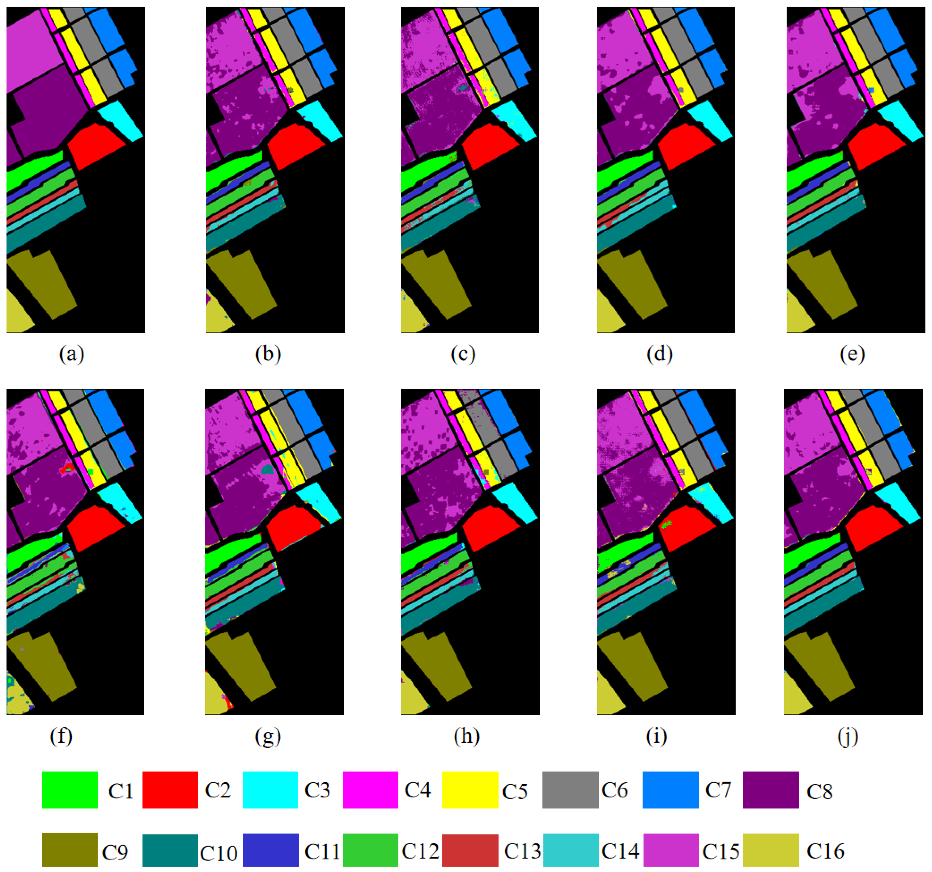
Figure 9. Ground-truth and classification maps of different methods on Salinas. (a) Ground-truth map. (b) SSFTT. (c) SpectralFormer. (d) Lite-HCNet. (e) GSC-ViT. (f) LSSAN. (g) CACFTNet. (h) MSDAN. (i) Sim Pool Former. (j) LSGMA.

As can be seen from the Table 4, on the Salinas dataset, LSGMA achieves superior classification accuracy compared to other methods in terms of three criteria. Particularly in comparison with LSSAN and CACFTNet, LSGMA significantly improves OA values and also achieves remarkable enhancements in AA and Kappa values. In addition, among the 16 classes, LSGMA achieves the highest classification accuracy for classes 4, 9, 10, 11, 13, 14, and 16 (fallow-rough-plow, soil-vinyard-develop, corn-senesced-green-weeds, lettuce-romaine-4wk, lettuce-romaine-6wk, lettuce-romaine-7wk, and vinyard-vertical-trellis).

Figure 9 shows the visual maps of various methods on the Salinas dataset. For convenient comparison, the ground-truth map of the Salinas dataset is presented first. From the perspective of these classification maps, the classification performance of the models proposed in recent years has been constrained by the limited training samples, and the classification maps still fail to achieve the ideal effect. The errors are mainly concentrated in Class 8 (grapes-untrained), which is frequently confused with Class 15 (vinyard-untrained). In addition, some methods also exhibit misclassification in other classes. For example, LSSAN misclassifies part of Class 8 (grapes-untrained) as Class 2 (brocoli-green-weeds-2), while CACFTNet misclassifies part of Class 8 as Class 10 (corn-senesced-green-weeds). In contrast, the classification map of the LSGMA shows higher class consistency and is the closest to the ground-truth map.

3.4.3. Result of QUH-Qingyun

The classification results of different methods on the QUH-Qingyun datasets are listed in Table 5 (the bold font in the table indicates the best performance among all the methods). The visual maps of the various methods are shown in Figure 10.

Table 5. Accuracy evaluation results of the QUH-Qingyun dataset.

Class	SSFTT	SpectralFormer	Lite-HCNet	Gsc-Vit	LSSAN	CACFTNet	MSDAN	SimPoolFormer	DEHF	LSGMA
1	95.05 ± 0.72	96.05 ± 0.94	95.75 ± 1.17	95.91 ± 2.10	95.08 ± 2.13	94.99 ± 1.27	95.66 ± 1.07	96.46 ± 2.49	95.18 ± 2.83	95.37 ± 0.50
2	88.98 ± 0.31	87.14 ± 1.14	90.36 ± 1.11	91.84 ± 1.26	91.34 ± 3.38	90.12 ± 2.64	88.83 ± 1.41	92.12 ± 0.91	94.22 ± 2.17	97.05 ± 0.56
3	0.02 ± 1.89	17.27 ± 2.31	34.08 ± 2.92	29.49 ± 0.76	3.25 ± 4.16	23.23 ± 9.35	2.01 ± 3.72	29.45 ± 7.08	44.95 ± 3.21	64.47 ± 1.02
4	95.41 ± 1.91	95.41 ± 2.10	97.56 ± 1.52	97.55 ± 3.05	98.06 ± 2.82	97.00 ± 3.98	97.91 ± 3.09	98.65 ± 1.67	97.63 ± 2.74	99.02 ± 0.43
5	89.66 ± 0.37	89.36 ± 0.31	92.75 ± 0.69	92.63 ± 0.78	93.83 ± 4.52	90.92 ± 0.59	91.71 ± 4.27	92.18 ± 1.33	94.81 ± 1.27	96.70 ± 0.30
6	89.21 ± 19.19	83.67 ± 8.29	91.57 ± 0.78	92.96 ± 6.44	87.48 ± 26.73	89.24 ± 6.37	88.18 ± 1.19	80.44 ± 13.57	91.61 ± 5.71	96.12 ± 9.07
OA%	89.75 ± 0.57	88.39 ± 0.70	92.06 ± 0.23	92.66 ± 0.30	90.76 ± 1.89	90.59 ± 1.05	90.12 ± 1.22	89.43 ± 1.22	93.26 ± 1.72	95.78 ± 0.28
AA%	76.39 ± 1.73	78.15 ± 0.94	83.68 ± 0.44	83.39 ± 0.60	78.17 ± 2.92	80.92 ± 1.85	77.05 ± 1.14	81.55 ± 1.59	86.40 ± 0.92	91.45 ± 0.47
Kappa%	86.35 ± 0.62	84.59 ± 0.75	89.45 ± 0.25	90.25 ± 0.32	87.73 ± 2.04	87.51 ± 1.14	86.85 ± 1.31	86.00 ± 1.33	91.06 ± 1.17	94.41 ± 4.33

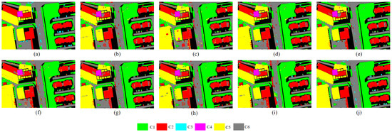
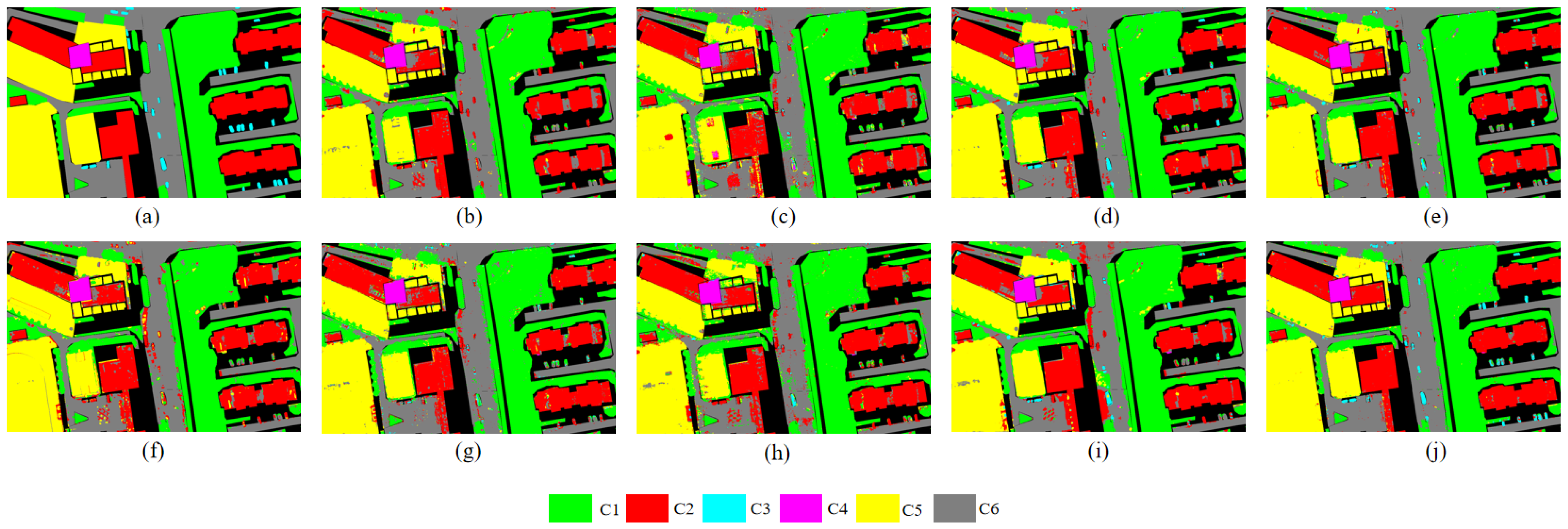
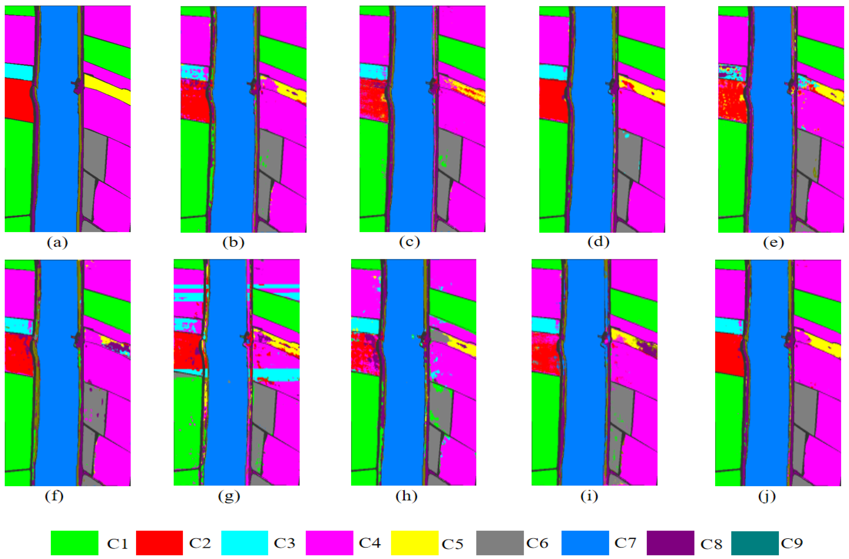
Figure 10. Ground-truth and classification maps of different methods on QUH-Qingyun. (a) Ground-truth map. (b) SSFTT. (c) SpectralFormer. (d) Lite-HCNet. (e) GSC-ViT. (f) LSSAN. (g) CACFTNet. (h) MSDAN. (i) Sim Pool Former. (j) LSGMA.

As can be seen from Table 5, on the QUH-Qingyun dataset, the proposed LSGMA achieves optimal performance across all three evaluation criteria. Compared with classical methods (e.g., SpectralFormer, LSSAN, and MSDAN) as well as representative models proposed in recent years (e.g., SSFTT, CACFTNet, and Sim Pool Former), LSGMA delivers OA improvements of over 3% in all cases, with the maximum improvement reaching 7.39%. Furthermore, among the six classes in this dataset, LSGMA attains the highest per-class accuracy in five classes. Particularly in Class 3 (car), which was partially obscured by shadows, the accuracy was significantly improved. These results demonstrate the superiority of the proposed method in identifying areas obscured by building shadows, highlighting the robustness of the approach.

The ground-truth map and the classification maps of different methods are shown in Figure 10. In the QUH-Qingyun dataset, certain regions are occluded by shadows cast by buildings and trees. Such shadow interference significantly degrades the classification accuracy of various mainstream methods. For example, methods such as SSFTT, Spectral, LSSAN, and MSDAN tend to misclassify the shadow-covered areas of Class 3 (car) as part of Class 2 (concrete building) or Class 1 (trees). Meanwhile, most methods also erroneously identify the areas of Class 6 (road) that are shaded by Class 1 (trees) as belonging to Class 1 (trees). In contrast, the LSGMA acquires global context through large kernel perception while accurately identifying shadow-affected regions through small kernel focusing, thereby improving classification accuracy and fully demonstrating the superiority of LSGMA in handling shadow interference.

3.4.4. Result of WHU-Hi-Longkou

The classification results of different methods on the WHU-Hi-Longkou dataset are listed in Table 6 (the bold font in the table indicates the best performance among all the methods), The visual maps of the variou.s methods are shown in Figure 11.

Table 6. Accuracy evaluation results of the WHU-Hi-Longkou Dataset.

Class	SSFTT	SpectralFormer	Lite-HCNet	Gsc-Vit	LSSAN	CACFTNet	MSDAN	SimPoolFormer	DEHF	LSGMA
1	99.64 ± 0.17	99.01 ± 0.68	99.91 ± 0.05	99.51 ± 0.48	98.00 ± 2.13	98.11 ± 1.56	98.39 ± 1.15	99.15 ± 0.64	99.60 ± 0.07	99.68 ± 0.10
2	82.14 ± 4.80	76.21 ± 10.33	95.21 ± 1.37	82.99 ± 11.01	73.61 ± 3.76	76.88 ± 12.54	78.33 ± 20.16	77.46 ± 8.57	71.75 ± 4.08	95.80 ± 1.72
3	64.58 ± 6.65	93.06 ± 2.72	95.18 ± 0.47	69.61 ± 35.71	65.29 ± 30.50	69.55 ± 15.26	91.10 ± 5.82	91.31 ± 7.81	78.41 ± 10.28	94.50 ± 1.07
4	99.00 ± 0.31	97.46 ± 0.60	99.23 ± 0.56	98.93 ± 0.39	96.71 ± 1.61	97.36 ± 1.18	98.68 ± 0.29	97.26 ± 1.23	98.32 ± 0.62	99.32 ± 0.29
5	51.00 ± 6.40	64.75 ± 7.11	74.71 ± 16.09	45.38 ± 21.02	50.68 ± 21.35	51.52 ± 26.95	65.60 ± 21.93	60.42 ± 16.49	55.88 ± 23.08	79.08 ± 9.58
6	98.3 ± 1.55	95.18 ± 2.67	98.31 ± 1.23	97.26 ± 1.87	95.44 ± 2.82	89.09 ± 4.42	92.90 ± 1.68	94.10 ± 4.63	95.00 ± 2.79	99.28 ± 0.15
7	99.67 ± 0.2	99.79 ± 0.28	99.89 ± 0.03	99.15 ± 0.55	99.15 ± 1.15	99.48 ± 0.40	99.62 ± 0.25	99.76 ± 0.13	99.62 ± 0.27	99.78 ± 0.21
8	74.37 ± 7.27	84.12 ± 6.77	90.98 ± 2.38	57.94 ± 12.70	49.49 ± 16.18	67.83 ± 14.35	81.90 ± 6.72	79.88 ± 12.68	87.42 ± 5.49	89.03 ± 5.25
9	56.9 ± 7.13	55.58 ± 6.36	66.16 ± 8.92	51.66 ± 24.72	53.50 ± 12.01	32.94 ± 18.47	51.03 ± 5.70	54.04 ± 9.28	56.35 ± 4.72	67.99 ± 5.41
OA%	95.24 ± 0.12	95.22 ± 0.47	97.65 ± 0.30	94.19 ± 0.77	92.56 ± 0.80	92.85 ± 1.10	95.19 ± 0.95	94.86 ± 0.40	95.07 ± 0.52	97.74 ± 0.31
AA%	80.9 ± 1.01	85.02 ± 1.20	91.06 ± 1.22	78.05 ± 3.60	75.76 ± 5.50	75.87 ± 3.75	84.17 ± 2.82	83.71 ± 2.08	82.48 ± 2.21	91.60 ± 1.74
Kappa%	93.69 ± 0.15	93.69 ± 0.62	96.91 ± 0.40	92.32 ± 1.02	90.22 ± 1.05	90.54 ± 1.47	93.65 ± 1.27	93.22 ± 0.52	93.49 ± 1.34	97.02 ± 0.41

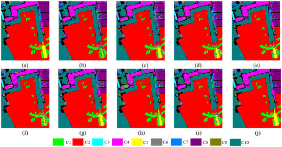
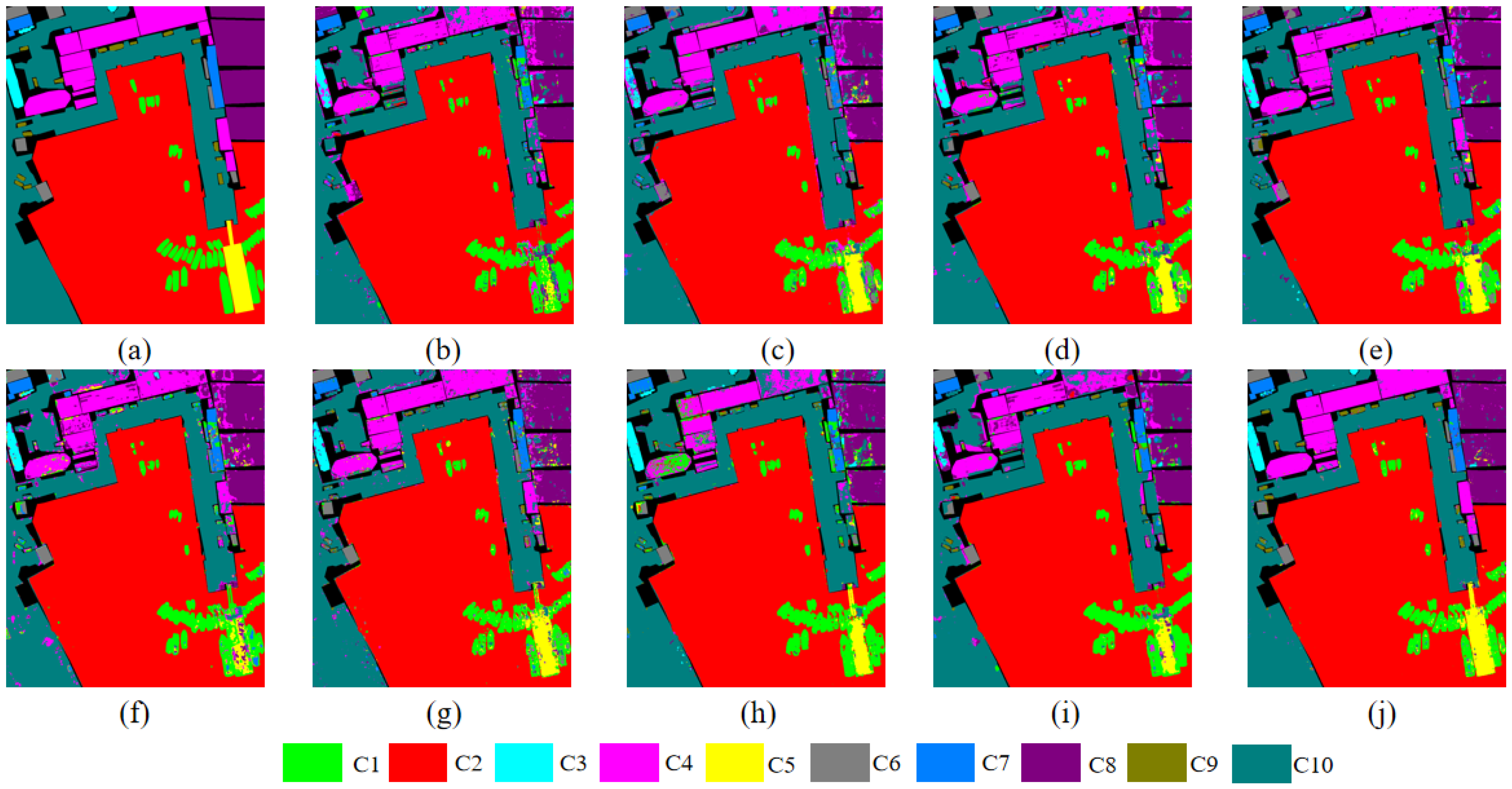
Figure 11. Ground-truth and classification maps of different methods on WHU-Hi-Longkou. (a) Ground-truth map. (b) SSFTT. (c) SpectralFormer. (d) Lite-HCNet. (e) GSC-ViT. (f) LSSAN. (g) CACFTNet. (h) MSDAN. (i) Sim Pool Former. (j) LSGMA.

As shown from Table 6, on the WHU-Hi-Longkou dataset, the LSGMA achieves the optimal classification performance across all evaluation criteria. In terms of AA values, the LSGMA shows significant improvements compared to GSC-ViT, LSSAN, and CACFTNet. Regarding OA values, it also surpasses several recently proposed mainstream models (e.g., CACFTNet, SSFTT, and SimPoolFormer), demonstrating further performance enhancement. Among the 8 classes of this dataset, the LSGMA achieves the highest classification accuracy in classes 2, 4, 5, 6, and 9 (cotton, broad-leaf soybean, narrow-leaf soybeans, rice, and mixed-weed).

Figure 11 intuitively shows the classification maps of different comparison methods. For ease of analysis, the ground-truth map is presented first. Across the classification maps, it is obvious that the classification maps of the comparison methods have deficiencies. In particular, Class 5 (narrow-leaf-soybeans), which is easily misclassified as Class 4 (broad-leaf-soybean) by most methods (e.g., SSFTT, SpectralFormer, LSSAN, and Lite-HCNet all exhibit this type of error). In addition, in LSSAN and SimPoolFormer, Class 5 is further misclassified as Class 8 (roads and houses). In rare cases, Class 5 is even mislabeled as Class 3 (sesame) or Class 6 (rice). In contrast, although the classification map generated by the LSGMA still has minor errors, it is the closest to the ground-truth map overall. This result further verifies the effectiveness and superiority of LSGMA in recognizing complex land-cover categories.

3.5. Ablation Study

To further analyze the importance of the MLA module and the LSGF module in the LSGMA, a series of ablation studies was conducted to verify the impact of these two modules on network performance.

As shown in Table 7, removing any single module from the LSGMA architecture leads to a significant degradation in all three evaluation metrics. This trend is consistently observed across the four datasets. Specifically, after removing the MLA module, OA decreases by 2.83%, 1.92%, 2.27%, and 2.27% on the four datasets, respectively; after removing the LSGF module, OA decreases by 2.48%, 2.05%, 2.55%, and 2.14%, respectively. Furthermore, for both average accuracy (AA) and the Kappa coefficient, the simultaneous removal of the two modules also results in substantial accuracy drops. The results indicate that both the MLA and LSGF modules can effectively enhance the model’s capability, and their synergistic effect can further strengthen the classification accuracy, exhibiting obvious complementary advantages. In summary, both the MLA and the LSGF make important contributions to improving the model’s classification performance, which verifies their effectiveness and complementarity.

Table 7. Results of the first and second ablation study.

Datasets	Moudle				OA	AA	Kappa	Params/K	FLOPs/K
	MLA		LSGF
	SA	CR	LKS	SKD
QUH-Pingan	√		√	√	95.48	85.58	93.25	20.627	322.003
		√	√	√	95.90	86.98	93.89	20.661	322.013
			√	√	94.59	81.92	91.92	20.527	321.974
	√	√	√		96.09	87.48	94.18	20.681	321.945
	√	√		√	95.86	87.62	93.86	20.679	321.965
	√	√			94.94	83.40	92.46	20.513	321.827
	√	√	√	√	97.42	92.34	96.15	20.705	322.178
Salinas	√		√	√	94.11	96.64	93.46	22.813	761.523
		√	√	√	93.94	96.26	93.26	22.806	761.501
			√	√	93.41	95.59	92.67	22.717	761.492
	√	√	√		93.97	96.22	93.30	22.760	761.561
	√	√		√	93.65	93.44	92.94	22.774	761.585
	√	√			93.28	92.21	92.53	22.699	761.450
	√	√	√	√	95.33	97.28	94.80	22.861	761.608
QUH-Qingyun	√		√	√	94.13	79.05	91.26	20.583	321.953
		√	√	√	94.45	88.58	92.65	20.571	322.001
			√	√	93.51	85.81	91.39	20.498	321.892
	√	√	√		93.94	86.77	91.96	20.462	321.894
	√	√		√	94.21	87.42	92.32	20.471	321.903
	√	√			93.23	85.49	91.01	20.412	321.785
	√	√	√	√	95.78	91.45	94.41	20.653	322.130
WHU-Hi-Longkou	√		√	√	95.88	84.79	94.56	23.875	539.628
		√	√	√	96.10	87.18	95.37	23.839	539.614
			√	√	95.38	84.15	93.90	23.764	539.571
	√	√	√		96.14	85.69	94.91	23.817	539.602
	√	√		√	96.23	89.08	95.03	23.791	539.578
	√	√			95.60	85.91	94.20	23.775	539.505
	√	√	√	√	97.74	91.61	97.02	23.902	539.648

In order to verify the contribution of the SA block and the CR block in the MLA module, as well as the LKS block and the SKD block in the LSGF module, in the presented approach to the ultimate classification result, the second-degree ablation study is carried out on the four datasets. The study results are presented in Table 7.

From the Table 7, we observe that removing either block within the MLA leads to a decline across all three evaluation criteria. The SA block is originally designed to better extract mid-level features overlooked by existing methods, thereby improving the network’s classification accuracy, while the CR block redistributes the input at the channel level to reduce information redundancy. When both blocks exist simultaneously, the MLA exhibits stronger feature integration capability, which further enhances the classification performance of the LSGMA. The results demonstrate that both the SA block and the CR block contribute substantially to performance improvements, which verifies their critical role in feature extraction and classification accuracy enhancement.

As clearly demonstrated in Table 7, both the LKS and SKD blocks in the LSGF module are crucial. Across all datasets, only when both blocks are present do all three evaluation metrics achieve their highest values. The LKS block employs large-kernel depth-wise convolutions to fully capture long-range spatial contextual information, ensuring comprehensive feature extraction and providing a rich semantic context for the subsequent steps. Building upon the information captured by LKS, the SKD block utilizes group-based small-kernel dynamic convolutions to dynamically assign weights to the critical central features. In summary, through the collaborative interaction between LKS and SKD, the module retains the advantages of global modeling while maintaining computational efficiency by focusing on key features. As illustrated in the Table 7, the cooperation of both blocks makes a significant contribution to improving the model’s classification accuracy, and the absence of either one leads to a decline in the model’s classification performance.

As shown in Table 7, simultaneously introducing LSGF and MLA modules leads to a moderate increase in the number of parameters and FLOPs, with a maximum increase of no more than 0.3%. However, the resulting gain in classification performance is more significant, with OA increasing by up to about 5%, while the model’s classification accuracy is significantly improved. This result demonstrates that extracting previously neglected intermediate-order features can effectively increase the model’s classification accuracy while maintaining the number of parameters.

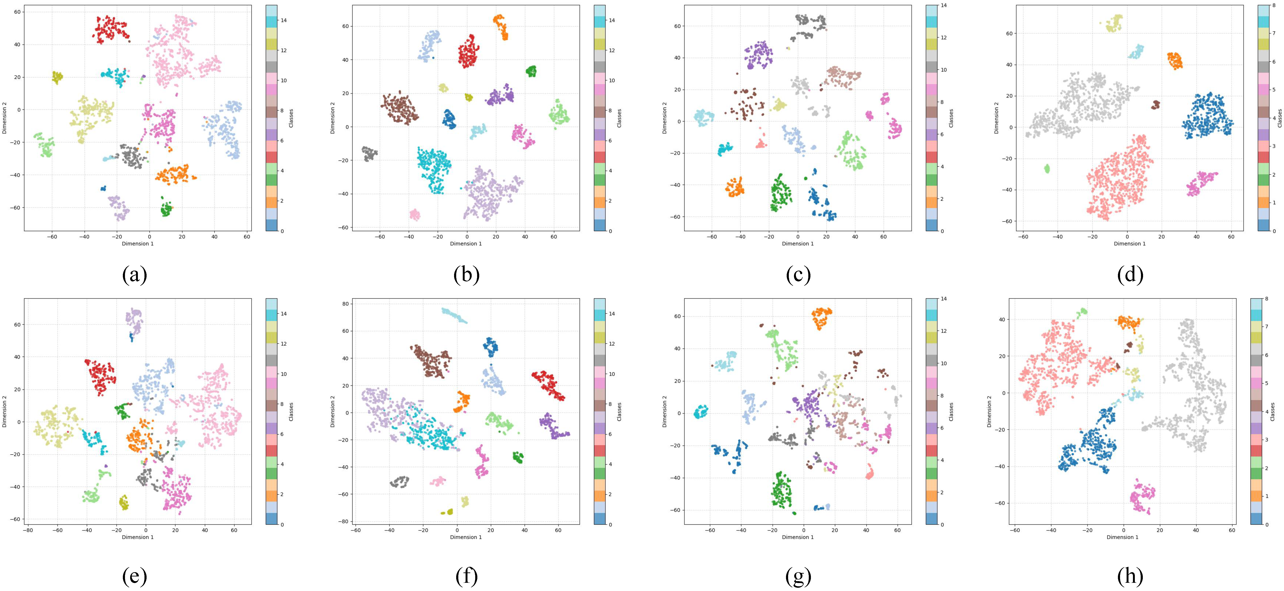
To more intuitively verify the role of mid-level interaction in the HSIC task, we removed the SA module used to extract mid-level interactions, thus eliminating the model’s ability to extract mid-level interactions. Based on this, we used t-SNE to visualize the features, clearly demonstrating the difference between the feature distributions obtained with and without mid-level interaction extraction by comparing them.

As can be observed in Figure 12, when mid-level features are not extracted, the data points of different classes are heavily mixed and overlap with each other. In contrast, after the extraction of mid-level features, data points from different classes are more clearly separated, while those belonging to the same class are clustered more tightly. This leads to a marked improvement in classification performance.

Figure 12. t-SNE visualizations of extracting mid-level features. (a) QUH-Pingan. (b) Salinas. (c) QUH-Qingyun. (d) WHU-Hi-Longkou. t-SNE visualizations of Unextracting mid-level features. (e) QUH-Pingan. (f) Salinas. (g) QUH-Qingyun. (h) WHU-Hi-Longkou.

4. Conclusions

In this article, an efficient and accurate HSIC network named LSGMA is proposed. First, considering the limitations of both patch-based and image-based input, we employ LKS to expand the receptive field and fully extract spatial contextual information. Then, SKD is adopted to adaptively aggregate central feature representations. The combination of these two components forms the LSGF. Second, we introduce the MLA to effectively integrate multi-level features. It encodes the previously neglected mid-level feature interactions through Spatial Aggregation (SA), and then performs channel-wise reallocation on the input via Channel Reallocation (CR). Finally, a series of parameter experiments and ablation studies are conducted, and comparative experiments are carried out with seven state-of-the-art classification methods on four public datasets. The results demonstrate that LSGMA exhibits superior performance in HSIC tasks.

References

- Ghamisi, P.; Plaza, J.; Chen, Y.; Li, J.; Plaza, A.J. Advanced spectral classifiers for hyperspectral images: A review. IEEE Geosci. Remote Sens. Mag. 2017, 5, 8–32. [Google Scholar] [CrossRef] [Scilit]
- Lu, G.; Fei, B. Medical hyperspectral imaging: A review. J. Biomed. Opt. 2014, 19, 010901. [Google Scholar] [CrossRef] [Scilit] [PubMed]
- Abbas, S.; Peng, Q.; Wong, M.S.; Li, Z.; Wang, J.; Ng, K.T.K.; Kwok, C.Y.T.; Hui, K.K.W. Characterizing and classifying urban tree species using bi-monthly terrestrial hyperspectral images in Hong Kong. ISPRS J. Photogramm. Remote Sens. 2021, 177, 204–216. [Google Scholar] [CrossRef] [Scilit]
- De Almeida, D.R.A.; Broadbent, E.N.; Ferreira, M.P.; Meli, P.; Zambrano, A.M.A.; Gorgens, E.B.; Resende, A.F.; de Almeida, C.T.; Do Amaral, C.H.; Dalla Corte, A.P.; et al. Monitoring restored tropical forest diversity and structure through UAV-borne hyperspectral and lidar fusion. Remote Sens. Environ. 2021, 264, 112582. [Google Scholar] [CrossRef] [Scilit]
- Ghiyamat, A.; Shafri, H.Z. A review on hyperspectral remote sensing for homogeneous and heterogeneous forest biodiversity assessment. Int. J. Remote Sens. 2010, 31, 1837–1856. [Google Scholar] [CrossRef] [Scilit]
- Kramer, S.J.; Siegel, D.A.; Maritorena, S.; Catlett, D. Modeling surface ocean phytoplankton pigments from hyperspectral remote sensing reflectance on global scales. Remote Sens. Environ. 2022, 270, 112879. [Google Scholar] [CrossRef] [Scilit]
- Melgani, F.; Bruzzone, L. Classification of hyperspectral remote sensing images with support vector machines. IEEE Trans. Geosci. Remote Sens. 2004, 42, 1778–1790. [Google Scholar] [CrossRef] [Scilit]
- Li, J.; Bioucas-Dias, J.M.; Plaza, A. Spectral–spatial hyperspectral image segmentation using subspace multinomial logistic regression and Markov random fields. IEEE Trans. Geosci. Remote Sens. 2011, 50, 809–823. [Google Scholar] [CrossRef] [Scilit]
- Prasad, S.; Bruce, L.M. Limitations of principal components analysis for hyperspectral target recognition. IEEE Geosci. Remote Sens. Lett. 2008, 5, 625–629. [Google Scholar] [CrossRef] [Scilit]
- Du, Q. Modified Fisher’s linear discriminant analysis for hyperspectral imagery. IEEE Geosci. Remote Sens. Lett. 2007, 4, 503–507. [Google Scholar]
- Wang, D.; Hu, M.; Jin, Y.; Miao, Y.; Yang, J.; Xu, Y.; Qin, X.; Ma, J.; Sun, L.; Li, C.; et al. HyperSIGMA: Hyperspectral intelligence comprehension foundation model. IEEE Trans. Pattern Anal. Mach. Intell. 2025, 47, 6427–6444. [Google Scholar] [CrossRef] [Scilit] [PubMed]
- Zhu, X.X.; Tuia, D.; Mou, L.; Xia, G.S.; Zhang, L.; Xu, F.; Fraundorfer, F. Deep learning in remote sensing: A comprehensive review and list of resources. IEEE Geosci. Remote Sens. Mag. 2017, 5, 8–36. [Google Scholar] [CrossRef] [Scilit]
- Li, S.; Song, W.; Fang, L.; Chen, Y.; Ghamisi, P.; Benediktsson, J.A. Deep learning for hyperspectral image classification: An overview. IEEE Trans. Geosci. Remote Sens. 2019, 57, 6690–6709. [Google Scholar] [CrossRef] [Scilit]
- Audebert, N.; Le Saux, B.; Lefèvre, S. Deep learning for classification of hyperspectral data: A comparative review. IEEE Geosci. Remote Sens. Mag. 2019, 7, 159–173. [Google Scholar] [CrossRef] [Scilit]
- Kang, X.; Wang, Z.; Duan, P.; Wei, X. The potential of hyperspectral image classification for oil spill mapping. IEEE Trans. Geosci. Remote Sens. 2022, 60, 5538415. [Google Scholar] [CrossRef] [Scilit]
- Kang, X.; Zhuo, B.; Duan, P. Dual-path network-based hyperspectral image classification. IEEE Geosci. Remote Sens. Lett. 2018, 16, 447–451. [Google Scholar]
- Chen, Y.; Lin, Z.; Zhao, X.; Wang, G.; Gu, Y. Deep learning-based classification of hyperspectral data. IEEE J. Sel. Top. Appl. Earth Obs. Remote Sens. 2014, 7, 2094–2107. [Google Scholar] [CrossRef] [Scilit]
- Yang, J.; Du, B.; Wang, D.; Zhang, L. ITER: Image-to-pixel representation for weakly supervised HSI classification. IEEE Trans. Image Process. 2023, 33, 257–272. [Google Scholar] [PubMed]
- Hu, W.; Huang, Y.; Wei, L.; Zhang, F.; Li, H. Deep convolutional neural networks for hyperspectral image classification. J. Sens. 2015, 2015, 258619. [Google Scholar] [CrossRef] [Scilit]
- Makantasis, K.; Karantzalos, K.; Doulamis, A.; Doulamis, N. Deep supervised learning for hyperspectral data classification through convolutional neural networks. In Proceedings of the 2015 IEEE International Geoscience and Remote Sensing Symposium (IGARSS), Milan, Italy, 26–31 July 2015; IEEE: New York, NY, USA, 2015; pp. 4959–4962. [Google Scholar]
- Liu, D.; Han, G.; Liu, P.; Yang, H.; Sun, X.; Li, Q.; Wu, J. A novel 2D-3D CNN with spectral-spatial multi-scale feature fusion for hyperspectral image classification. Remote Sens. 2021, 13, 4621. [Google Scholar]
- Yang, J.; Du, B.; Xu, Y.; Zhang, L. Can spectral information work while extracting spatial distribution?—An online spectral information compensation network for HSI classification. IEEE Trans. Image Process. 2023, 32, 2360–2373. [Google Scholar] [CrossRef] [Scilit] [PubMed]
- Yang, J.; Du, B.; Wu, C. Lgformer: Local-to-global transformer for hyperspectral image classification. In Proceedings of the IGARSS 2023-2023 IEEE International Geoscience and Remote Sensing Symposium, Pasadena, CA, USA, 16–21 July 2023; IEEE: New York, NY, USA, 2023; pp. 5938–5941. [Google Scholar]
- Zhang, J.; Wei, F.; Feng, F.; Wang, C. Spatial–spectral feature refinement for hyperspectral image classification based on attention-dense 3D-2D-CNN. Sensors 2020, 20, 5191. [Google Scholar] [PubMed]
- Feng, F.; Wang, S.; Wang, C.; Zhang, J. Learning deep hierarchical spatial–spectral features for hyperspectral image classification based on residual 3D-2D CNN. Sensors 2019, 19, 5276. [Google Scholar] [CrossRef] [Scilit]
- Yu, L.; Zhang, X.; Wang, K. CMAAC: Combining multiattention and asymmetric convolution global learning framework for hyperspectral image classification. IEEE Trans. Geosci. Remote Sens. 2024, 62, 5508518. [Google Scholar] [CrossRef] [Scilit]
- Zheng, Z.; Zhong, Y.; Ma, A.; Zhang, L. FPGA: Fast patch-free global learning framework for fully end-to-end hyperspectral image classification. IEEE Trans. Geosci. Remote Sens. 2020, 58, 5612–5626. [Google Scholar] [CrossRef] [Scilit]
- Yu, H.; Zhang, H.; Liu, Y.; Zheng, K.; Xu, Z.; Xiao, C. Dual-channel convolution network with image-based global learning framework for hyperspectral image classification. IEEE Geosci. Remote Sens. Lett. 2021, 19, 6005705. [Google Scholar]
- Zhu, Q.; Deng, W.; Zheng, Z.; Zhong, Y.; Guan, Q.; Lin, W.; Zhang, L.; Li, D. A spectral-spatial-dependent global learning framework for insufficient and imbalanced hyperspectral image classification. IEEE Trans. Cybern. 2021, 52, 11709–11723. [Google Scholar]
- Deng, H.; Ren, Q.; Zhang, H.; Zhang, Q. Discovering and explaining the representation bottleneck of dnns. arXiv 2021, arXiv:2111.06236. [Google Scholar]
- Ancona, M.; Oztireli, C.; Gross, M. Explaining deep neural networks with a polynomial time algorithm for shapley value approximation. In Proceedings of the International Conference on Machine Learning (ICML), Long Beach, CA, USA, 9–15 June 2019; pp. 272–281. [Google Scholar]
- Zhang, H.; Li, S.; Ma, Y.; Li, M.; Xie, Y.; Zhang, Q. Interpreting and boosting dropout from a game-theoretic view. arXiv 2020, arXiv:2009.11729. [Google Scholar]
- Cheng, X.; Chu, C.; Zheng, Y.; Ren, J.; Zhang, Q. A game-theoretic taxonomy of visual concepts in dnns. arXiv 2021, arXiv:2106.10938. [Google Scholar]
- Fu, H.; Sun, G.; Zhang, L.; Zhang, A.; Ren, J.; Jia, X.; Li, F. Three-dimensional singular spectrum analysis for precise land cover classification from UAV-borne hyperspectral benchmark datasets. ISPRS J. Photogramm. Remote Sens. 2023, 203, 115–134. [Google Scholar]
- Green, R.O.; Eastwood, M.L.; Sarture, C.M.; Chrien, T.G.; Aronsson, M.; Chippendale, B.J.; Faust, J.A.; Pavri, B.E.; Chovit, C.J.; Solis, M.; et al. Imaging spectroscopy and the airborne visible/infrared imaging spectrometer (AVIRIS). Remote Sens. Environ. 1998, 65, 227–248. [Google Scholar] [CrossRef] [Scilit]
- Zhong, Y.; Hu, X.; Luo, C.; Wang, X.; Zhao, J.; Zhang, L. WHU-Hi: UAV-borne hyperspectral with high spatial resolution (H2) benchmark datasets and classifier for precise crop identification based on deep convolutional neural network with CRF. Remote Sens. Environ. 2020, 250, 112012. [Google Scholar]
- Sun, L.; Zhao, G.; Zheng, Y.; Wu, Z. Spectral–spatial feature tokenization transformer for hyperspectral image classification. IEEE Trans. Geosci. Remote Sens. 2022, 60, 5522214. [Google Scholar] [CrossRef] [Scilit]
- Hong, D.; Han, Z.; Yao, J.; Gao, L.; Zhang, B.; Plaza, A.; Chanussot, J. SpectralFormer: Rethinking hyperspectral image classification with transformers. IEEE Trans. Geosci. Remote Sens. 2021, 60, 5518615. [Google Scholar] [CrossRef] [Scilit]
- Ma, X.; Kang, X.; Qin, H.; Wang, W.; Ren, G.; Wang, J.; Liu, B. A Lightweight Hybrid Convolutional Neural Network for Hyperspectral Image Classification. IEEE Trans. Geosci. Remote Sens. 2023, 61, 5513714. [Google Scholar] [CrossRef] [Scilit]
- Zhao, Z.; Xu, X.; Li, S.; Plaza, A. Hyperspectral image classification using groupwise separable convolutional vision transformer network. IEEE Trans. Geosci. Remote Sens. 2024, 62, 5511817. [Google Scholar] [CrossRef] [Scilit]
- Cui, Y.; Xia, J.; Wang, Z.; Gao, S.; Wang, L. Lightweight spectral–spatial attention network for hyperspectral image classification. IEEE Trans. Geosci. Remote Sens. 2021, 60, 5510114. [Google Scholar] [CrossRef] [Scilit]
- Cheng, S.; Chan, R.; Du, A. CACFTNet: A hybrid cov-attention and cross-layer fusion transformer network for hyperspectral image classification. IEEE Trans. Geosci. Remote Sens. 2024, 62, 1–17. [Google Scholar]
- Wang, X.; Fan, Y. Multiscale densely connected attention network for hyperspectral image classification. IEEE J. Sel. Top. Appl. Earth Obs. Remote Sens. 2022, 15, 1617–1628. [Google Scholar] [CrossRef] [Scilit]
- Roy, S.K.; Jamali, A.; Chanussot, J.; Ghamisi, P.; Ghaderpour, E.; Shahabi, H. SimPoolFormer: A two-stream vision transformer for hyperspectral image classification. Remote Sens. Appl. Soc. Environ. 2025, 37, 101478. [Google Scholar]
- Zhang, J.; Wang, J.; Li, D.; Zhang, J.; Sun, X.; Shang, X. Hyperspectral Band Selection with Dynamic Graph Enhancement and Hierarchical Feature Fusion. IEEE Trans. Geosci. Remote Sens. 2026, 64, 5508816. [Google Scholar] [CrossRef] [Scilit]
Disclaimer/Publisher’s Note: The statements, opinions and data contained in all publications are solely those of the individual author(s) and contributor(s) and not of MDPI and/or the editor(s). MDPI and/or the editor(s) disclaim responsibility for any injury to people or property resulting from any ideas, methods, instructions or products referred to in the content. |
© 2026 by the authors. Licensee MDPI, Basel, Switzerland. This article is an open access article distributed under the terms and conditions of the Creative Commons Attribution (CC BY) license.