A Superpixel-Guided Spectral–Spatial Fusion Network for Hyperspectral Scene Classification

Highlights

What are the main findings?

• We propose a superpixel-guided spectral aggregation strategy that represents hyperspectral images using compact, boundary-aware spectral tokens, which are then combined with a pretrained spectral foundation model and a pseudo-RGB branch to achieve efficient spectral–spatial feature fusion.
• A lightweight adaptation strategy is applied to transfer the pretrained spectral model, enabling stable performance improvement in hyperspectral scene classification under limited labeled samples.

What are the implications of the main findings?

• The results suggest that organizing hyperspectral observations according to spatially coherent structures is beneficial for improving performance of hyperspectral scene classification.
• The findings indicate that lightweight adaptation of pretrained spectral priors can stabilize HSI-SC under scarce supervision and better exploit high-dimensional spectral information.

Abstract

In recent years, research on remote sensing scene classification (RSSC) has mainly focused on high-resolution imagery, which provides limited spectral information, whereas hyperspectral imaging (HSI) offers richer cues about material properties and compositional structure. Despite its potential, hyperspectral scene classification (HSI-SC) remains challenging because pixel- or patch-based representations fail to preserve spatial structures and regional boundaries. In addition, labeled hyperspectral samples are often scarce, making it difficult to learn stable class-discriminative representations from high-dimensional spectral observations. To address these issues, this paper proposes a dual-branch fusion framework. Superpixels are used to aggregate high-dimensional spectral signals into compact, boundary-aware tokens. The spectral branch is initialized with pretrained model weights and further adapted via a lightweight adaptation strategy for efficient transfer under limited supervision. In parallel, a pseudo-RGB spatial branch complements structural and textural information. Spectral and spatial features are fused additively to generate a more discriminative scene representation. Experimental results demonstrate that the proposed method outperforms compared hyperspectral scene classification approaches.

1. Introduction

Hyperspectral scene classification (HSI-SC) aims to assign a semantic category to each hyperspectral scene by considering its spatial layout, land cover composition, and continuous spectral responses [1], and has become an important technique for urban planning, precision agriculture, and disaster monitoring [2]. Traditional HSI-SC studies have mainly focused on RGB or multispectral imagery, where scene recognition relies primarily on spatial textures, structural patterns, and geometric features [3]. However, in complex scenarios such as high-density urban areas and agro-forestry transition zones, regions with different functions may exhibit similar visual appearances. As a result, methods that rely only on spatial–visual cues are prone to visual ambiguity [4]. In contrast, hyperspectral imaging (HSI) records fine-grained spectral responses over continuous wavelengths, providing physically meaningful information related to material properties and compositional differences. Such spectral evidence can help alleviate visual ambiguity and improve scene-level semantic discrimination [5,6]. Accordingly, hyperspectral scene classification (HSI-SC) has attracted increasing research attention.

Despite the rich spectral information provided by HSI, HSI-SC remains challenging [7]. Unlike pixel-wise land cover classification, scene classification requires a model to capture not only local material responses, but also the compositional relationships, spatial arrangement, and overall appearance of the scene. Conventional pixel-level or fixed patch-based representations often introduce excessively long input sequences and tend to cut across object or material boundaries, making it difficult to preserve spatially coherent structures. In addition, hyperspectral data acquisition and scene-level annotation are costly, so labeled hyperspectral scene samples are often limited. Under such restricted supervision, directly learning stable class-discriminative representations from high-dimensional spectral observations remains difficult.

To address these issues, this paper proposes a superpixel-guided spectral–spatial fusion network for HSI-SC. The proposed method first uses superpixels to organize a hyperspectral image into spatially coherent units, where each unit is represented by its mean spectrum. This design reduces the number of input tokens while preserving boundary-aware local structures. The resulting spectral tokens are encoded by a pretrained spectral branch, and a lightweight adaptation strategy is adopted to transfer spectral knowledge to the downstream scene classification task. Meanwhile, a pseudo-RGB spatial branch is introduced to provide complementary texture and shape cues. Finally, the spectral and pseudo-RGB features are fused to obtain a more discriminative scene representation.

2. Related Work

2.1. Feature Learning for Remote Sensing Scene Classification

Early studies on remote sensing scene classification mainly relied on handcrafted feature descriptors. These methods used manually designed feature extraction strategies to describe local textures, edge structures, and spectral statistical distributions. Representative descriptors include Local Binary Patterns (LBPs), Scale-Invariant Feature Transform (SIFT), and Histograms of Oriented Gradients (HOGs) [8]. Although these methods can be effective in relatively simple scenes, their representation capacity is limited by their dependence on expert knowledge, making it difficult to characterize complex spatial configurations, regional compositions, and high-level semantic information.

To reduce the dependence on handcrafted descriptors, data-driven unsupervised feature learning methods were introduced to learn more adaptive representations from unlabeled pixels or low-level features. Typical methods include Principal Component Analysis (PCA) [9], Independent Component Analysis (ICA) [10], sparse coding [11], and shallow autoencoders (AEs) [12]. These methods can capture latent statistical patterns and improve feature expressiveness. However, because they usually lack explicit scene-level semantic supervision, the learned representations may not be well aligned with scene discrimination objectives, especially when inter-class differences are subtle and intra-class variations are complex.

With the rapid development of deep learning [13,14,15], CNN-, RNN-, and Transformer-based models have been widely used for remote sensing and hyperspectral image interpretation. CNNs provide strong local feature extraction ability [16,17,18,19,20,21], RNNs can model sequential dependencies [22], and Transformers are effective in capturing long-range interactions through self-attention [23,24,25]. Within these advanced paradigms, distinct feature-modeling paradigms have been developed to handle high-dimensional remote sensing observations. For instance, spectral embedding blocks are typically utilized at the initial input layer as a tokenization mechanism, focusing on mapping raw spectral dimensions into a continuous latent space to align features for subsequent layers. Whereas the multi-convolutional modulator designed in the THSGR framework [26], operate deep within the network backbone to model long-range structural dependencies and cross-modal interactions; by employing self-attention-free gated convolutions. Driven by these diverse architectural designs, numerous advanced scene representation models have been proposed. For example, Chen et al. [27] introduced GCSANet by embedding global context spatial attention into DenseNet to enhance contextual representation. Zhao et al. [28] developed MGML-FENet to integrate multi-granularity and multi-level features for capturing both local details and high-level semantics. Tang et al. [29] proposed ACNet to improve the robustness of spatial attention by enforcing attention consistency between original and rotated images. Other studies have explored structured key-area localization [30], covariance-based representation [31], self-supervised contrastive learning [32], self-attention-based feature aggregation [23], convolutional capsule networks [33], and fully contextual modeling [34] for remote sensing or hyperspectral classification tasks.

Although these methods have improved feature extraction and scene representation, they still face several limitations. First, many models rely on dense pixel-level or fixed patch-level representations, which may increase sequence length and computational cost when modeling global scene semantics. Second, the high costs of hyperspectral data acquisition and scene-level annotation often lead to limited training samples, making models susceptible to sample insufficiency and reducing result stability [35,36].

More recently, state space model based Mamba architectures have attracted increasing attention in hyperspectral image classification because of their ability to model long-range dependencies with linear computational complexity. For example, MambaHSI introduces spatial–spectral Mamba modeling for hyperspectral image classification [37], S2Mamba develops a spatial–spectral state space model for spectral–spatial feature fusion [38], and 3DSS-Mamba further explores three-dimensional spectral–spatial Mamba modeling for hyperspectral image classification [39]. These studies demonstrate the potential of Mamba-based models for efficient hyperspectral representation learning. However, most existing Mamba-based methods are still designed for pixel-level or patch-level hyperspectral classification, where the input is usually organized as regular image patches or spectral–spatial sequences. For hyperspectral scene classification, how to organize the full image into compact and boundary-aware units, and how to combine spectral representation with spatial appearance cues under limited supervision, remains insufficiently explored.

2.2. Pretraining and Foundation Models for Hyperspectral Representation

Pretraining has become an important strategy for improving representation learning under limited supervision. In remote sensing scene classification, a common practice is to adopt generic backbone networks pretrained on large-scale RGB datasets, such as ResNet [40] and ViT [41], as feature extractors. However, these models are mainly pretrained on natural images and therefore tend to emphasize local textures and spatial structures. Due to the substantial differences between RGB images and hyperspectral images in imaging mechanisms, inter-band correlations, and data distributions, their transferability to hyperspectral scene classification remains constrained.

To better model the intrinsic characteristics of hyperspectral data, hyperspectral foundation models have recently been developed. HyperSIGMA [42] proposes a spatial–spectral dual-branch foundation model tailored for hyperspectral data, introducing sparse sampling attention and a spectral enhancement module on top of large-scale pretraining to strengthen the joint modeling of spatial features and spectral information. HyperFree [43] incorporates a visual prompting mechanism for channel-wise adaptation. By constructing a learnable weight dictionary over the wavelength range of $0.4$–$2.5\mathsf{\mu }\mathrm{m}$, it enables dynamic adaptation to inputs with different band configurations. SpectralEarth [44] establishes a large-scale hyperspectral dataset with global coverage and multi-temporal characteristics based on EnMAP [45]. HyperSL [46] maps spectral signals from different sensors into a unified sequential representation through a universal spectral tokenizer and wavelength positional encoding.

These studies have provided important foundations for hyperspectral representation learning. Nevertheless, existing hyperspectral foundation model research still mainly focuses on pixel-level or patch-level interpretation. For HSI-SC, the modeling of regional compositional relationships and global spatial organization remains relatively limited. Therefore, it is necessary to develop a framework that preserves boundary-aware regional information, reduces modeling complexity, and integrates transferable spectral knowledge with spatial appearance cues for scene-level classification.

3. Methodology

3.1. Problem Definition and Overall Architecture

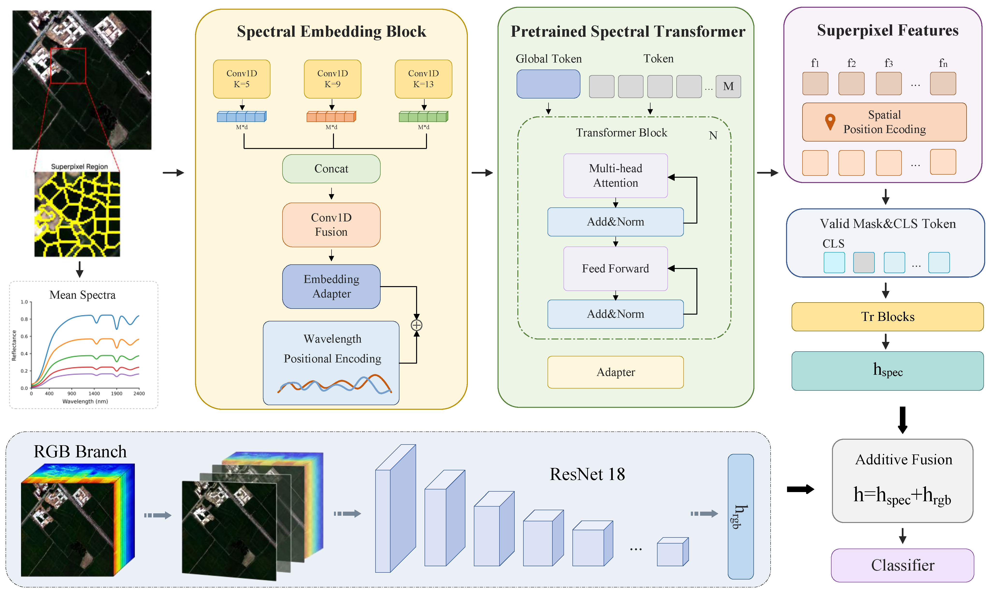
Hyperspectral scene classification differs fundamentally from pixel-wise land cover classification. Instead of predicting a label for each individual pixel, it assigns a semantic category to an entire hyperspectral image patch. Consequently, a reliable model should account not only for local material responses, but also for the composition of multiple regions, their spatial arrangement, and the overall appearance of the scene. Motivated by these requirements, we develop a dual-branch framework that combines spectral modeling with pseudo-RGB spatial representation learning. The overall architecture of the proposed framework is shown in Figure 1.

Given a hyperspectral image patch

$$\mathbf{X}\in {\mathbb{R}}^{H\times W\times C},$$

(1)

where H, W, and C denote the image height, image width, and number of spectral bands, respectively, and a wavelength vector

$$\mathsf{\lambda }=[{\lambda }_1,{\lambda }_2,\dots ,{\lambda }_C]\in {\mathbb{R}}^C,$$

(2)

where ${\lambda }_c$ denotes the physical wavelength of the c-th spectral band, the goal of hyperspectral scene classification is to learn a mapping

$$\widehat{y}=f_{\mathrm{\Theta }}(\mathbf{X},\mathsf{\lambda }),$$

(3)

where $\widehat{y}\in \{1,2,\dots ,M\}$ is the predicted scene label, M is the number of scene categories, and $\mathsf{\Theta }$ denotes the learnable parameters of the proposed framework.

The proposed method organizes a hyperspectral image into a compact set of superpixels, where each superpixel is represented by its mean spectrum. These spectra are encoded by a pretrained wavelength-aware spectral encoder to extract discriminative spectral features. The centroid of each superpixel is further used to retain spatial layout information, and Transformer integrates the valid superpixel features for image-level classification. In parallel, a pseudo-RGB branch extracts complementary texture and shape cues from the hyperspectral cube. The final prediction is obtained by additive fusion of the spectral and pseudo-RGB features followed by a classification head.

3.2. Superpixel-Based Region Construction

The input organization begins with a superpixel partition, which defines the spatial units used to compute superpixel spectra and centroid coordinates.

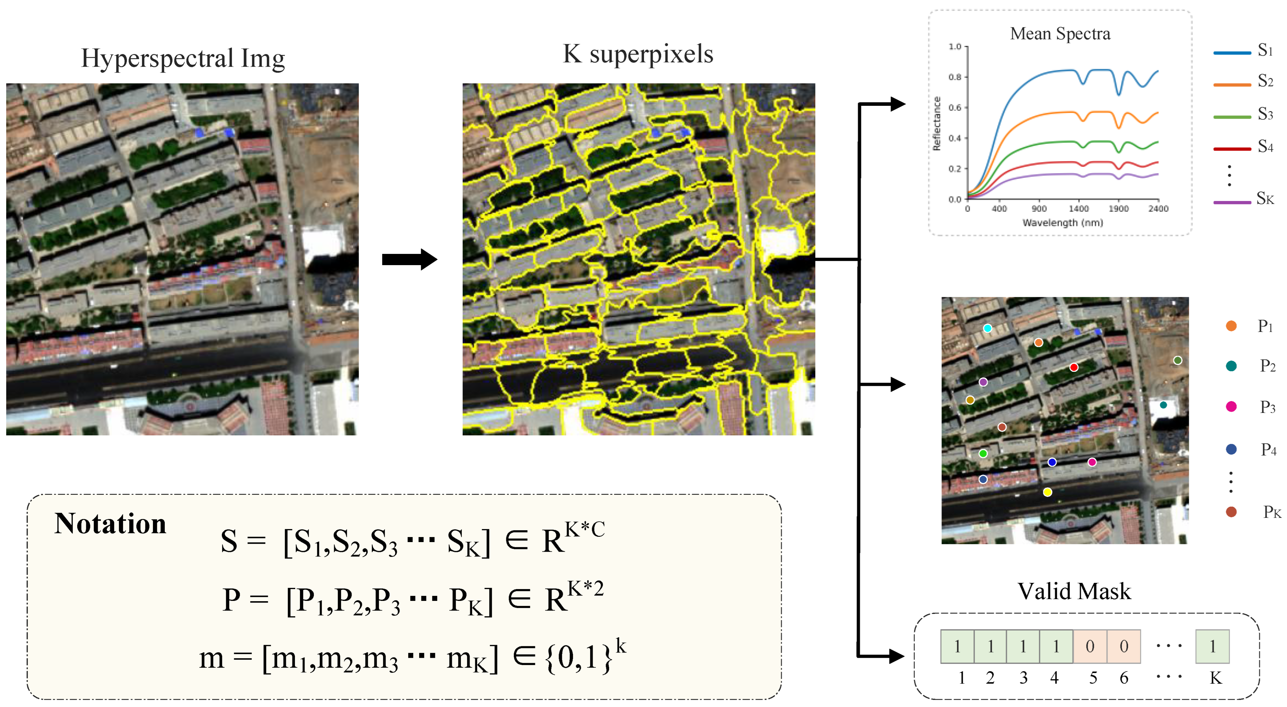
Directly using all pixels in a hyperspectral patch would produce a long input sequence and may mix pixels from different objects or materials. To obtain a more compact input while better preserving local spatial consistency, Simple Linear Iterative Clustering(SLIC) is applied to aggregate the image into spatially coherent superpixels. The superpixel-based region construction process is shown in Figure 2.

Let the resulting superpixel label map be

$$\mathbf{L}\in {\{0,1,\dots ,N-1\}}^{H\times W},$$

(4)

where N denotes the actual number of superpixels in the current image patch, and $L_{u,v}$ is the superpixel index assigned to pixel $(u,v)$.

The pixel set associated with the i-th superpixel is defined as

$${\mathsf{\Omega }}_i=\{(u,v)\mid L_{u,v}=i\},i=0,1,\dots ,N-1.$$

(5)

Here, ${\mathsf{\Omega }}_i$ denotes the set of spatial coordinates belonging to the i-th superpixel, and $|{\mathsf{\Omega }}_i|$ denotes the number of pixels within this region.

After the spatial regions are obtained, each superpixel is further summarized by its representative spectral response.

For each superpixel, the mean spectrum of all pixels within the region is used as its representative spectral descriptor. The c-th spectral component of the i-th superpixel is computed as

$$s_i\left(c\right)={\displaystyle \frac{1}{|{\mathsf{\Omega }}_i|}}\sum _{(u,v)\in {\mathsf{\Omega }}_i}{X}_{u,v,c},c=1,2,\dots ,C.$$

(6)

In this equation, $X_{u,v,c}$ denotes the spectral response at spatial coordinate $(u,v)$ and spectral band c, while $s_i\left(c\right)$ denotes the average response of the i-th superpixel at the same band.

The corresponding spectral vector is written as

$${\mathbf{s}}_i={[s_i\left(1\right),s_i\left(2\right),\dots ,s_i\left(C\right)]}^{\top }\in {\mathbb{R}}^C.$$

(7)

By stacking all spectra, the spectral set representation is obtained as

$$\mathbf{S}={[{\mathbf{s}}_0,{\mathbf{s}}_1,\dots ,{\mathbf{s}}_{N-1}]}^{\top }\in {\mathbb{R}}^{N\times C}.$$

(8)

Here, each row of $\mathbf{S}$ corresponds to the mean spectrum of one superpixel region.

In addition to spectral information, the spatial location of each superpixel is retained to describe the regional layout of the scene.

To preserve the spatial organization of superpixel regions, the centroid of each superpixel is further computed. The row and column coordinates of the centroid of the i-th superpixel are defined as

$$p_i^u={\displaystyle \frac{1}{|{\mathsf{\Omega }}_i|}}\sum _{(u,v)\in {\mathsf{\Omega }}_i}u,p_i^v={\displaystyle \frac{1}{|{\mathsf{\Omega }}_i|}}\sum _{(u,v)\in {\mathsf{\Omega }}_i}v.$$

(9)

Here, $p_i^u$ and $p_i^v$ denote the row-wise and column-wise centroid coordinates, respectively.

To remove the influence of image size, the centroid coordinates are normalized by the spatial dimensions:

$${\tilde{p}}_i^u={\displaystyle \frac{p_i^u}{H}},{\tilde{p}}_i^v={\displaystyle \frac{p_i^v}{W}}.$$

(10)

The normalized centroid coordinates therefore lie in the range $[0,1)$ under the current implementation.

The normalized position vector of the i-th superpixel is then written as

$${\mathbf{p}}_i=[{\tilde{p}}_i^u,{\tilde{p}}_i^v]\in {\mathbb{R}}^2.$$

(11)

By stacking all region centroids, the position matrix is obtained as

$$\mathbf{P}={[{\mathbf{p}}_0,{\mathbf{p}}_1,\dots ,{\mathbf{p}}_{N-1}]}^{\top }\in {\mathbb{R}}^{N\times 2}.$$

(12)

Each row of $\mathbf{P}$ corresponds to the centroid of one superpixel region.

Since the number of superpixels varies across different image patches, the variable-length region set must be converted into a fixed-length representation for mini-batch training. Let K denote the predefined maximum number of region tokens. The spectral matrix and position matrix are padded to

$${\mathbf{S}}_{\mathrm{pad}}\in {\mathbb{R}}^{K\times C},{\mathbf{P}}_{\mathrm{pad}}\in {\mathbb{R}}^{K\times 2}.$$

(13)

A binary validity mask is simultaneously constructed as

$$\mathbf{m}\in {\{0,1\}}^K,$$

(14)

where

$$m_i=\left\{\begin{array}{cc}1,\hfill & i<N,\hfill \\ 0,\hfill & i\ge N,\hfill \end{array}\right.i=0,1,\dots ,K-1.$$

(15)

In this definition, $m_i=1$ indicates that the i-th token corresponds to a valid superpixel, whereas $m_i=0$ indicates that it is a padded token.

Accordingly, each hyperspectral patch is converted into the triplet

$$\left({\mathbf{S}}_{\mathrm{pad}},{\mathbf{P}}_{\mathrm{pad}},\mathbf{m}\right),$$

(16)

which serves as the input to the spectral branch.

3.3. Pretrained Spectral Prior for Encoding

After obtaining the spectra of the superpixels, we introduce a pretrained spectral encoder to extract spectral features from these one-dimensional inputs. Unlike methods that encode two-dimensional hyperspectral patches, the proposed spectral branch takes each superpixel spectrum as an independent spectral sequence. This input form is well aligned with HyperSL, whose pretraining is based on one-dimensional spectral tokenization and wavelength-aware encoding. Therefore, HyperSL is used to initialize the spectral branch, providing a compatible pretrained prior for subsequent task adaptation.

Each superpixel spectrum is then transformed into a sequence of band-wise tokens before being fed into the spectral encoder.

Given the representative spectrum ${\mathbf{s}}_i\in {\mathbb{R}}^C$ of the i-th superpixel, the first step is to convert it into a band-token sequence using multi-scale one-dimensional convolutions. Three parallel branches with kernel sizes 5, 9, and 13 are employed to capture local spectral contexts at different receptive fields:

$${\mathbf{e}}_i^{\left(1\right)}={\mathsf{\Phi }}_5\left({\mathbf{s}}_i\right)\in {\mathbb{R}}^{D\times C},$$

(17)

$${\mathbf{e}}_i^{\left(2\right)}={\mathsf{\Phi }}_9\left({\mathbf{s}}_i\right)\in {\mathbb{R}}^{D\times C},$$

(18)

$${\mathbf{e}}_i^{\left(3\right)}={\mathsf{\Phi }}_{13}\left({\mathbf{s}}_i\right)\in {\mathbb{R}}^{D\times C}.$$

(19)

In the above equations, D denotes the embedding dimension. ${\mathsf{\Phi }}_5(·)$, ${\mathsf{\Phi }}_9(·)$, and ${\mathsf{\Phi }}_{13}(·)$ denote three independent one-dimensional convolutional modules with kernel sizes of 5, 9, and 13, respectively. Each module consists of a Conv1D layer, a BatchNorm1D layer, and a GELU activation.

The outputs of the three branches are concatenated along the channel dimension and fused by a $1\times 1$ convolution:

$${\mathbf{E}}_i={\mathsf{\Phi }}_{1\times 1}\left([{\mathbf{e}}_i^{\left(1\right)};{\mathbf{e}}_i^{\left(2\right)};{\mathbf{e}}_i^{\left(3\right)}]\right)\in {\mathbb{R}}^{D\times C}.$$

(20)

Here, $[·;·]$ denotes channel-wise concatenation, and ${\mathsf{\Phi }}_{1\times 1}(·)$ denotes the fusion module implemented by a $1\times 1$ Conv1D, followed by BatchNorm1D and GELU.

The fused feature map is then transposed into token-sequence form:

$${\mathbf{Z}}_i={\mathbf{E}}_i^{\top }\in {\mathbb{R}}^{C\times D}.$$

(21)

In this representation, the c-th row of ${\mathbf{Z}}_i$ corresponds to the D-dimensional token associated with the c-th spectral band.

To further enhance the adaptability of the embedded spectral tokens, an embedding-level Adapter is inserted after the spectral embedding stage:

$${\overline{\mathbf{Z}}}_i={\mathbf{Z}}_i+{\mathcal{A}}_{\mathrm{emb}}\left({\mathbf{Z}}_i\right).$$

(22)

Here, ${\mathcal{A}}_{\mathrm{emb}}(·)$ denotes the embedding-level Adapter, and the residual formulation allows task-specific adjustment of spectral tokens before deeper encoding.

After the embedding-level adaptation, wavelength-aware positional information is added to the spectral token sequence.

Each spectral band corresponds to a physical wavelength rather than a purely ordinal index. To preserve this property, wavelength-aware positional encoding is introduced. First, the wavelength of the c-th band is normalized as

$${\overline{\lambda }}_c={\displaystyle \frac{{\lambda }_c-400}{10}},c=1,2,\dots ,C.$$

(23)

Here, ${\overline{\lambda }}_c$ denotes the normalized wavelength value used by the encoding function.

Following the current implementation, the frequency coefficient of the t-th sine-cosine pair is defined as

$${\alpha }_t=exp\left(-{\displaystyle \frac{log100}{D}}·2t\right),t=0,1,\dots ,{\displaystyle \frac{D}{2}}-1.$$

(24)

In this equation, ${\alpha }_t$ is the frequency coefficient for the t-th embedding dimension pair.

The wavelength-aware positional encoding matrix ${\mathbf{P}}^{\lambda }\in {\mathbb{R}}^{C\times D}$ is then given by

$$P_{c,2t}^{\lambda }=sin\left({\alpha }_t{\overline{\lambda }}_c\right),P_{c,2t+1}^{\lambda }=cos\left({\alpha }_t{\overline{\lambda }}_c\right).$$

(25)

Here, $P_{c,2t}^{\lambda }$ and $P_{c,2t+1}^{\lambda }$ denote the sine and cosine components of the positional encoding assigned to the c-th band.

The wavelength-aware token sequence is thus obtained as

$${\tilde{\mathbf{Z}}}_i={\overline{\mathbf{Z}}}_i+{\mathbf{P}}^{\lambda }.$$

(26)

This operation injects physical wavelength information into the embedded spectral tokens.

With the wavelength-aware tokens prepared, the spectral Transformer backbone is then used to encode the spectral sequence.

A global token inherited from the pretrained spectral backbone is prepended to the sequence:

$${\mathbf{H}}_i^0=\left[\mathbf{g};{\tilde{\mathbf{Z}}}_i\right]\in {\mathbb{R}}^{(C+1)\times D}.$$

(27)

Here, $\mathbf{g}\in {\mathbb{R}}^D$ denotes the inherited global token, and ${\mathbf{H}}_i^0$ denotes the initial input sequence of the i-th region.

Let ${\mathcal{B}}_{\ell }(·)$ denote the ℓ-th spectral Transformer block and let ${\mathcal{A}}_{\ell }(·)$ denote the Adapter attached after that block. The encoding process is formulated as

$${\tilde{\mathbf{H}}}_i^{\ell }={\mathcal{B}}_{\ell }\left({\mathbf{H}}_i^{\ell -1}\right),\ell =1,2,\dots ,L_s,$$

(28)

$${\mathbf{H}}_i^{\ell }={\tilde{\mathbf{H}}}_i^{\ell }+{\mathcal{A}}_{\ell }\left({\tilde{\mathbf{H}}}_i^{\ell }\right),\ell =1,2,\dots ,L_s,$$

(29)

where $L_s$ denotes the number of spectral Transformer blocks.

The final spectral feature is extracted from the first output token:

$${\mathbf{f}}_i={\mathbf{H}}_i^{L_s}\left(0\right)\in {\mathbb{R}}^D.$$

(30)

That is, ${\mathbf{f}}_i$ denotes the encoded spectral feature of the i-th superpixel.

To preserve the pretrained spectral knowledge while enabling downstream adaptation, the spectral branch is trained using a lightweight transfer strategy.

Rather than fully fine-tuning the pretrained spectral backbone, a lightweight adaptation strategy is adopted. In the current implementation, the spectral embedding layers, the inherited global token, and the pretrained spectral Transformer blocks are frozen. The normalization layers remain trainable. In addition, all Adapter modules, the superpixel position encoder, the pseudo-RGB branch, and the classification head are optimized. This design is intended to preserve pretrained spectral priors while allowing efficient adaptation to scene classification.

3.4. Transformer-Based Global Context Modeling

After each superpixel has been encoded into a spectral feature vector, the model further incorporates its spatial location to preserve the layout of the superpixel distribution. Specifically, the centroid coordinate of the i-th superpixel is projected into the same feature space as the spectral feature:

$${\mathsf{\pi }}_i=\varphi \left({\mathbf{p}}_i\right)\in {\mathbb{R}}^D,$$

(31)

where $\varphi (·)$ denotes the superpixel position encoder, ${\mathbf{p}}_i$ is the normalized centroid coordinate of the i-th superpixel, and ${\mathsf{\pi }}_i$ is the corresponding position embedding.

The position-enhanced superpixel feature is then defined as

$${\widehat{\mathbf{f}}}_i={\mathbf{f}}_i+{\mathsf{\pi }}_i.$$

(32)

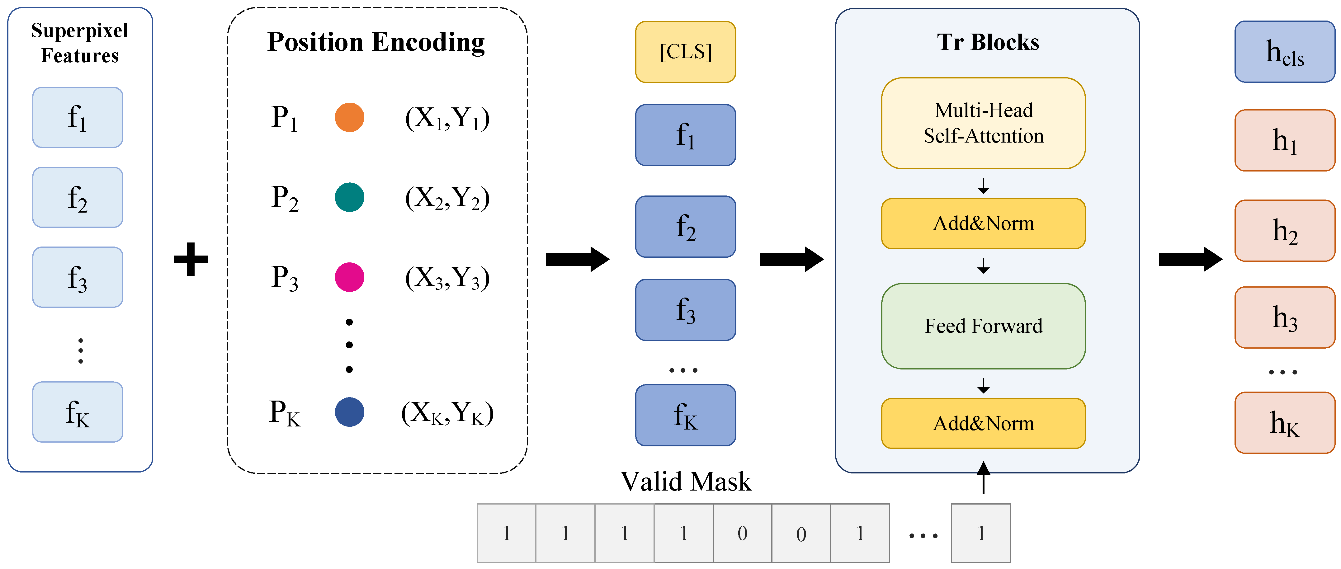
This operation injects spatial layout information into the spectral features of individual superpixels. The superpixel-level context aggregation module is shown in Figure 3.

All superpixel features are stacked into

$$\widehat{\mathbf{F}}={[{\widehat{\mathbf{f}}}_0,{\widehat{\mathbf{f}}}_1,\dots ,{\widehat{\mathbf{f}}}_{K-1}]}^{\top }\in {\mathbb{R}}^{K\times D},$$

(33)

where $\widehat{\mathbf{F}}$ denotes the sequence of position-enhanced superpixel features.

To obtain a representation from the token sequence, a learnable classification token is introduced for global semantic aggregation.

To aggregate global semantics from all valid superpixel tokens, a learnable classification token is prepended to the input sequence:

$${\mathbf{U}}^0=[\mathbf{c};\widehat{\mathbf{F}}]\in {\mathbb{R}}^{(K+1)\times D},$$

(34)

where $\mathbf{c}\in {\mathbb{R}}^D$ is the cls token. During self-attention, this token interacts with all valid superpixel tokens and serves as the carrier of global scene semantics.

Since padded superpixel tokens may exist in the fixed-length sequence, the validity mask is first extended as

$${\mathbf{m}}^{\prime }=[1,m_0,m_1,\dots ,m_{K-1}]\in {\{0,1\}}^{K+1},$$

(35)

where the first element is set to 1 because the cls is always valid.

An additive attention mask is then defined as

$$a_j=\left\{\begin{array}{cc}0,\hfill & m_j^{\prime }=1,\hfill \\ -\infty ,\hfill & m_j^{\prime }=0,\hfill \end{array}\right.j=0,1,\dots ,K.$$

(36)

Here, $a_j$ denotes the additive penalty associated with the j-th token in attention computation. This mask is broadcast to the attention logits so that padded tokens do not participate in effective token interactions.

Let ${\mathcal{F}}_{\ell }(·;\mathbf{a})$ denote the ℓ-th Transformer block under additive attention mask $\mathbf{a}$. The global context modeling process is formulated as

$${\mathbf{U}}^{\ell }={\mathcal{F}}_{\ell }\left({\mathbf{U}}^{\ell -1};\mathbf{a}\right),\ell =1,2,\dots ,L_c,$$

(37)

where $L_c$ denotes the number of Transformer blocks.

After aggregation, the output corresponding to the classification token is used as the feature of the spectral branch

$${\mathbf{h}}_{\mathrm{spec}}={\mathbf{U}}^{L_c}\left(0\right)\in {\mathbb{R}}^D.$$

(38)

This vector is used as the final spectral-branch representation of the entire hyperspectral scene.

3.5. Pseudo-RGB Spatial Branch and Dual-Branch Fusion

The spectral branch provides the hyperspectral representation ${\mathbf{h}}_{\mathrm{spec}}$ through superpixel-based spectral tokenization, pretrained spectral encoding, and global context aggregation. Alongside the spectral branch, a pseudo-RGB spatial branch is introduced to extract complementary texture and structural cues from the visible-band information of the hyperspectral cube.

Specifically, three spectral bands closest to the red, green, and blue wavelengths are selected:

$$r=\arg \underset{j}{\min }|{\lambda }_j-650|,g=\arg \underset{j}{\min }|{\lambda }_j-550|,b=\arg \underset{j}{\min }|{\lambda }_j-475|.$$

(39)

Here, r, g, and b denote the indices of the bands used to form the red, green, and blue channels, respectively. The pseudo-RGB image is then defined as

$${\mathbf{X}}^{\mathrm{rgb}}=\left[{\mathbf{X}}_{:,:,r},{\mathbf{X}}_{:,:,g},{\mathbf{X}}_{:,:,b}\right]\in {\mathbb{R}}^{H\times W\times 3}.$$

(40)

This image is entirely derived from the hyperspectral input and does not introduce additional RGB data.

The pseudo-RGB image is fed into a ResNet-18 backbone pretrained on ImageNet to extract spatial appearance features. To make its output compatible with the spectral representation, the original fully connected layer of ResNet-18 is replaced with a linear projection layer whose output dimension is D. The pseudo-RGB feature is denoted as

$${\mathbf{h}}_{\mathrm{rgb}}={\psi }_{\mathrm{rgb}}\left({\mathbf{X}}^{\mathrm{rgb}}\right)\in {\mathbb{R}}^D,$$

(41)

where ${\psi }_{\mathrm{rgb}}(·)$ denotes the modified ResNet-18 branch.

Given ${\mathbf{h}}_{\mathrm{spec}}\in {\mathbb{R}}^D$ and ${\mathbf{h}}_{\mathrm{rgb}}\in {\mathbb{R}}^D$, the two branch features are fused by element-wise addition:

$$\mathbf{h}={\mathbf{h}}_{\mathrm{spec}}+{\mathbf{h}}_{\mathrm{rgb}}.$$

(42)

The fused feature is then fed into the classification head to obtain the logits:

$$\mathbf{z}=g_{\mathrm{cls}}\left(\mathbf{h}\right)\in {\mathbb{R}}^M,$$

(43)

where $g_{\mathrm{cls}}(·)$ denotes the classification head and M is the number of scene categories.

The predicted probability of the m-th category is computed by

$$p_m={\displaystyle \frac{exp\left(z_m\right)}{{\sum }_{q=1}^{M}exp\left(z_q\right)}},m=1,2,\dots ,M.$$

(44)

Here, $z_m$ denotes the logit of the m-th class, and $p_m$ denotes the corresponding posterior probability.

The final scene label is obtained as

$$\widehat{y}=\arg \underset{m}{\max }{p}_m.$$

(45)

Thus, $\widehat{y}$ is the category with the highest predicted probability.

3.6. Optimization Objective

Let ${\mathbf{z}}_b=[z_{b,1},z_{b,2},\dots ,z_{b,M}]$ denote the logits of the b-th sample in a mini-batch of size B, and let $y_b$ denote its ground-truth scene label. The overall training objective is defined as the cross-entropy classification loss:

$$\mathcal{L}={\mathcal{L}}_{\mathrm{cls}}=-{\displaystyle \frac{1}{B}}{\displaystyle \sum _{b=1}^B}log{\displaystyle \frac{exp\left(z_{b,y_b}\right)}{{\sum }_{m=1}^{M}exp\left(z_{b,m}\right)}},$$

(46)

where $z_{b,y_b}$ denotes the logit corresponding to the ground-truth class of the b-th sample, and ${\mathcal{L}}_{\mathrm{cls}}$ is the average classification loss over the mini-batch.

4. Experiments

4.1. Datasets

To evaluate the effectiveness of different architectures under varying information inputs, experiments were conducted on two widely used standard hyperspectral scene classification datasets.

4.1.1. HSRS-SC Dataset [47]

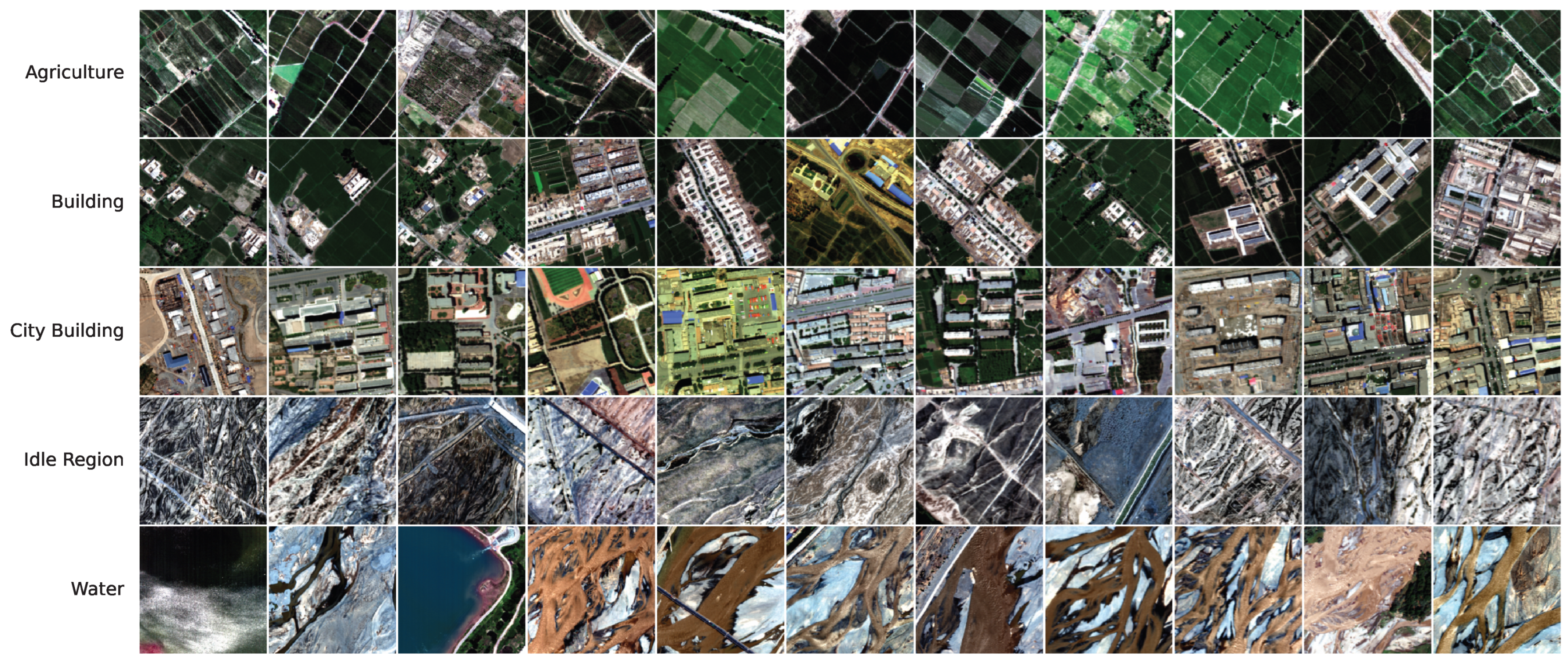
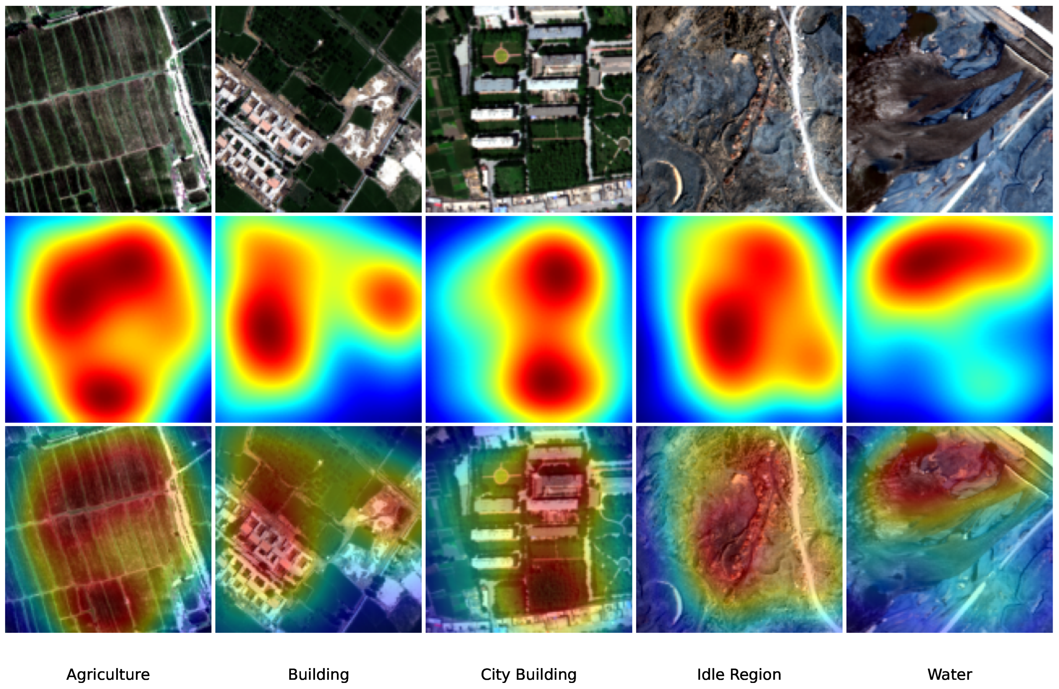
The HSRS-SC is a large-scale hyperspectral scene classification dataset derived from aerial data collected during the Heihe Watershed Allied Telemetry Experimental Research (HiWATER) mission. It comprises 1385 hyperspectral images with a spatial dimension of $256\times 256$ pixels. The dataset features a high spatial resolution of 1 m and a spectral range of 380 to 1050 nm across 48 bands. It is organized into five distinct categories, and representative samples are shown in Figure 4:

4.1.2. HRSSC Dataset [48]

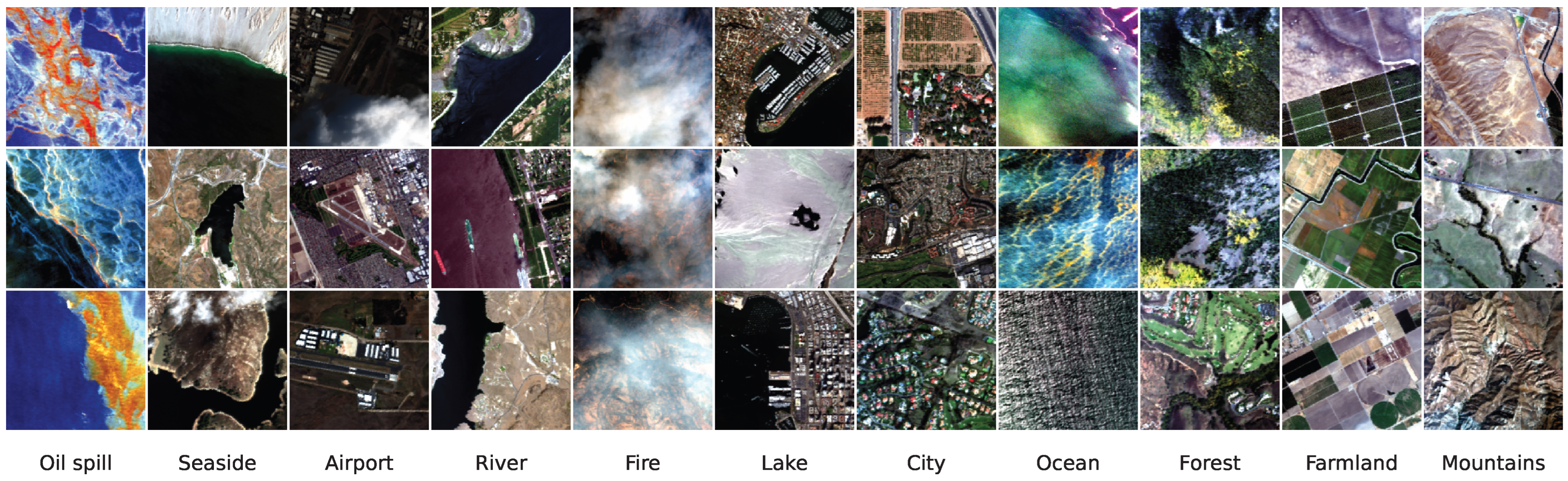
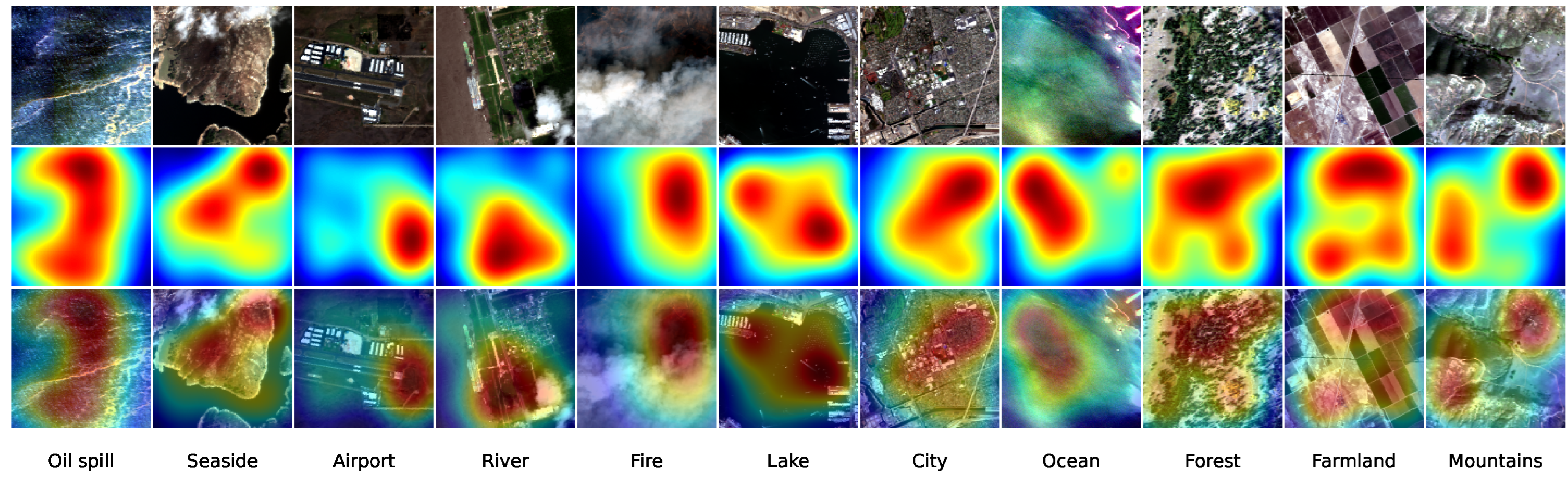
The HRSSC dataset is a high-resolution benchmark designed to evaluate scene classification performance using the Airborne Visible/Infrared Imaging Spectrometer (AVIRIS) sensor. This dataset consists of 1445 hyperspectral cubes with a spatial size of $256\times 256$ pixels and an extensive spectral depth of 224 bands spanning from 400 to 2500 nm. The spatial resolution varies from 3 to 15 m. The dataset includes 11 diverse categories: Airport, City, Farmland, Fire, Forest, Lake, Mountains, Ocean, Oil spill, River, and Seaside. Representative samples are shown in Figure 5.

4.2. Experimental Methodology

Four representative deep learning architectures were selected as baselines to benchmark performance. AlexNet [49] and ResNet-18 [40] were adopted as CNN baselines to represent early convolutional feature learning and deeper residual modeling, respectively. In addition, ViT [41] was included to capture global context through patch tokenization and self-attention, while DeiT [50] was used to assess the benefit of distillation-based training. Based on these four models, three distinct input schemes were designed to evaluate the contribution of different information types:

(a)

Scheme 1 (RGB): Utilizes three visible bands to generate RGB pseudo-color images, serving as a baseline to evaluate classification performance based primarily on spatial textures.

(b)

Scheme 2 (RGB+NIR): Extends Scheme 1 by incorporating three Near-Infrared (NIR) bands. Features are integrated via concatenation to assess the discriminative gain from non-visible spectral cues.

(c)

Scheme 3 (Fusion): Integrates RGB visual features with global spectral and joint spatial-spectral representations derived from the full hyperspectral data.

4.3. Experimental Setup

(a)

Hardware: Experiments were run on a high-performance server equipped with an Intel Xeon Platinum 8470Q processor (25 vCPUs), 32 GB RAM, and an NVIDIA RTX 5090 GPU.

(b)

Training Configuration: Pretrained weights for the four baseline models were sourced from the official torchvision library. Models were trained for 300 epochs using the AdamW [51] optimizer, which updates weights only for parameters that require gradients. The hyperparameters were set as follows: an initial learning rate of $1\times {10}^{-4}$, a weight decay coefficient of $5\times {10}^{-4}$, and $({\beta }_1,{\beta }_2)=(0.9,0.95)$.

(c)

Evaluation Metrics: Model performance is evaluated using Overall Accuracy (OA), Average Accuracy (AA), Kappa coefficient, and F1-score. OA measures the proportion of correctly classified samples among all test samples, while AA denotes the mean classification accuracy across all categories. Kappa evaluates the agreement between predictions and ground-truth labels by considering chance agreement, and F1-score provides a balanced measure of precision and recall. These metrics are reported to provide a comprehensive assessment of classification performance.

4.4. Results and Analysis

To evaluate model generalization under limited labeled samples, we adopted a random sampling strategy that selected only 10 samples per class for training, with all remaining labeled samples used for testing. All images were resized to $224\times 224$ pixels to meet the input requirements of the baseline networks. As reported in

Table 1. Results on HSRS-SC and HRSSC with different methods. All metrics are reported in %.

Method	HSRS-SC				HRSSC
	OA	AA	Kappa	F1	OA	AA	Kappa	F1
ViT (RGB)	93.78	93.33	91.88	93.76	78.28	75.10	74.93	79.89
DeiT (RGB)	89.36	88.33	86.02	89.04	68.01	64.79	63.24	69.97
AlexNet (RGB)	86.52	84.99	82.25	86.10	69.44	60.75	64.41	68.98
ResNet (RGB)	94.38	93.56	92.62	94.32	81.57	77.20	78.64	82.21
ViT (RGB+NIR)	94.83	94.42	93.23	94.82	78.50	75.79	75.28	80.44
DeiT (RGB+NIR)	94.61	93.66	92.91	94.52	75.06	75.26	71.29	76.88
AlexNet (RGB+NIR)	91.76	91.17	89.20	91.72	71.01	63.69	66.36	71.15
ResNet (RGB+NIR)	95.36	94.24	93.89	95.31	82.85	77.45	80.04	83.20
ViT (Fusion)	91.69	91.64	89.12	91.64	68.99	61.01	63.60	69.16
DeiT (Fusion)	93.41	92.73	91.35	93.35	70.94	67.08	66.16	71.67
AlexNet (Fusion)	94.91	93.79	93.30	94.82	76.48	74.30	72.72	76.47
ResNet (Fusion)	95.06	95.14	93.54	95.09	79.33	74.73	76.12	80.13
Ours	97.15	96.77	96.27	97.15	83.52	81.28	80.88	84.22

and

Table 2. Quantitative results of the proposed method with different hyperspectral foundation model weights on the HSRS-SC and HRSSC datasets. All metrics are reported in %.

Pre-Trained Weights	HSRS-SC				HRSSC
	OA	AA	Kappa	F1	OA	AA	Kappa	F1
HyperSIGMA	94.38	93.47	92.63	94.32	76.55	74.30	72.72	74.47
SpectralEarth	95.66	94.94	94.29	95.60	80.15	78.06	77.06	81.23
HyperFree	96.10	95.46	94.89	96.03	80.82	78.51	77.77	81.37
HyperSL	97.15	96.77	96.27	97.15	83.52	81.28	80.88	84.22

, the proposed method attains the highest values for all four metrics on both datasets under the current experimental setting. Under the 10-shot setting, the results in Table 1 indicate that performance is influenced not only by the amount of input information, but also by how that information is organized and matched to the backbone under limited supervision. The proposed method achieves the best overall performance on both datasets, suggesting that, in hyperspectral scene classification with limited samples, simply increasing the number of input channels is insufficient; the manner in which spectral and spatial cues are represented and integrated is equally important.

A consistent improvement is observed when moving from Scheme 1 to Scheme 2. Across all four backbones, the inclusion of NIR bands leads to better results on both datasets. This trend suggests that the additional near-infrared information provides complementary cues beyond those contained in an RGB-like representation. For remote sensing scene classification, scene categories are determined not only by visual appearance, but also by the material properties of the constituent regions. The fact that this trend is shared by all evaluated backbones further indicates that the contribution of NIR information is stable under the current protocol. By contrast, the effect of Scheme 3 is not consistent across architectures. Although AlexNet benefits from the Fusion setting, ViT, DeiT, and ResNet do not consistently outperform their corresponding RGB+NIR variants. This result suggests that the main difficulty lies not in whether richer hyperspectral information is useful, but in whether it can be transformed into a representation that remains learnable when only a small number of labeled samples is available. When the fusion process is not designed to organize spectral information in a manner aligned with scene recognition, the additional information may not translate into improved classification performance. Under the present setup, this issue appears to be more evident for generic visual backbones, particularly Transformer-based models, whose effectiveness is closely related to the way input tokens are formed and interpreted.

The comparison among backbones further supports this observation. ResNet provides the strongest competing performance in most settings, indicating that convolutional inductive biases remain effective for scene classification under limited supervision. Meanwhile, AlexNet achieves a more substantial performance gain under Scheme 3, indicating that the efficacy of feature fusion is not uniform across different settings. Taken together, these results indicate that the benefit of additional spectral information in hyperspectral scene classification with limited training samples depends not only on the information itself, but also on how it is structured, aggregated, and incorporated into the learning process.

To further examine the decision behavior of the proposed framework, we visualize class activation responses on HSRS-SC and HRSSC, as shown in Figure 6 and Figure 7. For each example, the first row shows the pseudo-RGB image, the second row presents the activation map, and the third row overlays the activation response on the pseudo-RGB image. The activation maps are generated from the final Transformer aggregation stage of the proposed model. Specifically, the target-class score is back-propagated to the superpixel tokens before the last aggregation block, and the resulting gradient-weighted token responses are mapped back to the image plane according to their corresponding superpixel locations. Therefore, the visualization indicates which image components contribute more strongly to the final prediction.

As shown in Figure 6, on HSRS-SC, the activation responses are generally concentrated on visually meaningful and category-relevant components. For agricultural scenes, the model tends to highlight regular field patterns; for building-related categories, stronger responses appear over constructed structures and their surrounding layouts; for water scenes, the activations are mainly distributed over homogeneous water surfaces and nearby boundaries. These observations indicate that the proposed model does not rely on isolated pixels or scattered background responses. Instead, it collects evidence from coherent image components that are closely related to the predicted category. This behavior is consistent with the superpixel-guided design, where hyperspectral pixels are first grouped into compact units before being processed by the spectral branch.

As shown in Figure 7, on HRSSC, the activation maps exhibit more diverse response patterns, which is reasonable given the larger number of categories and more heterogeneous image content in this dataset. The model tends to focus on category-related components, such as runways or open built-up structures in airport scenes, dense urban layouts in city scenes, vegetation-covered areas in farmland and forest scenes, and water bodies or shoreline structures in lake, river, ocean, and seaside scenes. Although HRSSC remains more challenging and contains stronger inter-class ambiguity, the activation responses are still mainly distributed over meaningful image components rather than irrelevant background areas. This observation is consistent with the quantitative results and confusion matrices, suggesting that the proposed spectral–spatial fusion framework can produce interpretable prediction evidence under limited supervision.

To examine the influence of different pretrained hyperspectral foundation model weights, we conducted an additional comparison by replacing only the pretrained initialization of the spectral branch while keeping the training strategy, classifier design, and evaluation protocol unchanged. Since the original foundation models differ in input organization, embedding design, and backbone structure, lightweight interface adaptations were applied when necessary so that the pretrained weights from HyperSIGMA [42], SpectralEarth [44], HyperFree [43], and HyperSL [46] could be incorporated into the same scene classification framework. Therefore, this experiment evaluates the transfer behavior of different pretrained weights within the proposed framework, rather than providing a direct comparison among the complete original foundation models.

On HSRS-SC [47], all four initialization sources achieve relatively high classification performance, with OA values ranging from 94.38% to 97.15%. Among them, HyperSL obtains the highest results, reaching 97.15% OA, 96.77% AA, 96.27 Kappa, and 97.15% F1-score. Compared with the second-best initialization, HyperFree, the corresponding improvements are 1.05, 1.31, 1.38, and 1.12 percentage points, respectively. This result indicates that, under the current experimental setting, the HyperSL initialization is the most compatible with the proposed spectral branch on HSRS-SC.

A similar trend can be observed on HRSSC [48]. HyperSL again achieves the highest values across all four metrics, with 83.52% OA, 81.28% AA, 80.88 Kappa, and 84.22% F1-score. The second-best results are obtained by HyperFree, which reaches 80.82% OA, 78.51% AA, 77.77 Kappa, and 81.37% F1-score. Thus, the gains of HyperSL over the second-best initialization are 2.70, 2.77, 3.11, and 2.85 percentage points in OA, AA, Kappa, and F1-score, respectively. The larger performance gap on HRSSC suggests that the choice of pretrained initialization has a more visible effect on this dataset under the current protocol.

The observed differences are consistent with the architectural relationship between the pretrained weights and the proposed spectral branch. In this work, the spectral branch processes region-level one-dimensional spectra obtained through superpixel aggregation. Therefore, pretrained weights derived from a model that explicitly encodes spectral sequences and incorporates wavelength-aware information can be more directly mapped to the proposed region-level spectral encoder. Under this setting, HyperSL provides a compatible initialization for the spectral encoder, since its pretraining formulation is also centered on one-dimensional spectral tokenization and wavelength-aware representation learning.The fundamental reason for the performance discrepancies among HyperSIGMA, SpectralEarth, HyperFree and HyperSL lies in their fundamentally different architectural assumptions at the design stage. For example, HyperSIGMA emphasizes spatial–spectral foundation modeling, SpectralEarth is built around spectral adaptation for large-scale hyperspectral pretraining, and HyperFree focuses on channel-adaptive and promptable hyperspectral inference. When their pretrained weights are adapted to the present framework, their original structural context cannot be preserved exactly. Consequently, the results in Table 1 reflect their performance after adaptation to the proposed scene classification pipeline, rather than the full capability of the original models.

Based on the above content, HyperSL is adopted as the default pretrained initialization for the spectral branch. This choice because its one-dimensional spectral tokenization and wavelength-aware representation are more consistent with the input form and encoding process used in the proposed method. Under the current framework, this compatibility reduces the architectural mismatch during weight transfer and leads to the best overall results on both HSRS-SC and HRSSC.

4.4.1. Confusion Matrix Analysis

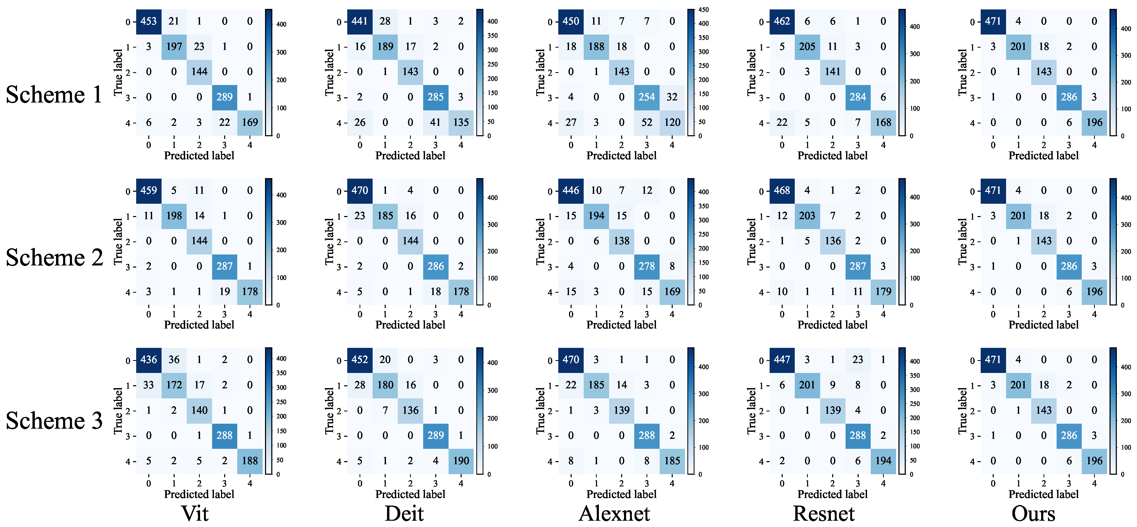
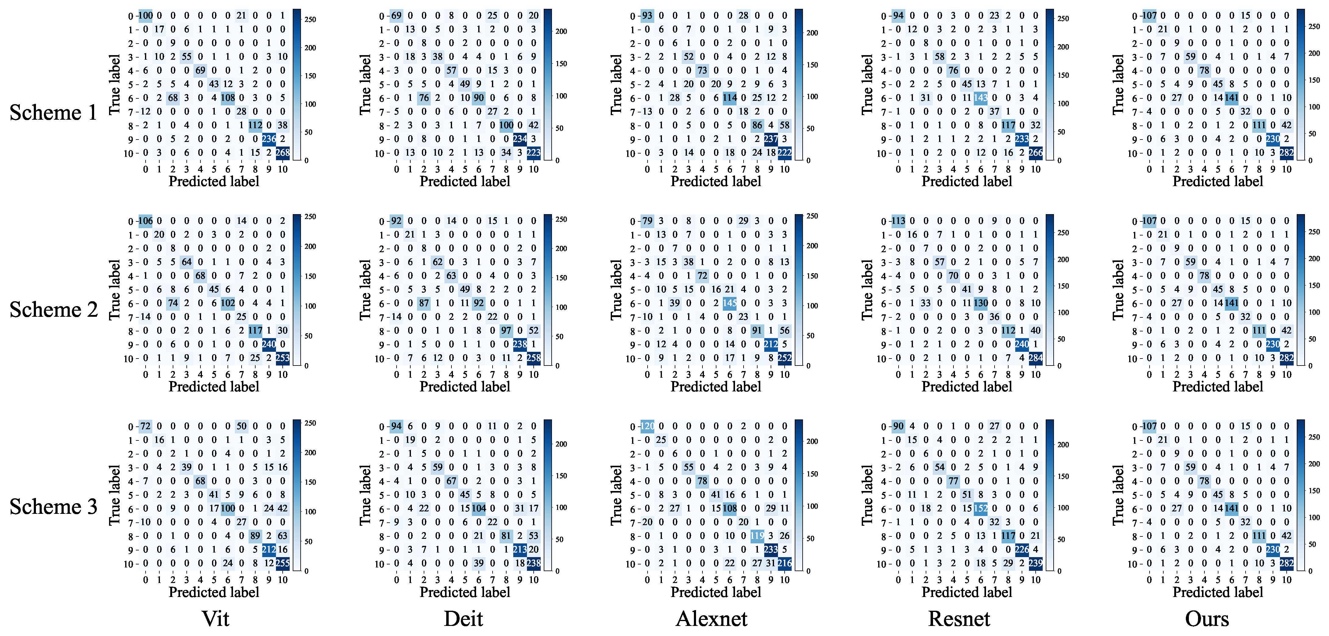
The confusion matrices in Figure 8 and Figure 9 provide a class-wise view of the prediction distributions under the three input schemes. Unlike OA, AA, Kappa, and F1-score, which summarize the overall classification performance, confusion matrices show how correctly and incorrectly classified samples are distributed across individual scene categories. A stronger concentration along the main diagonal indicates that more samples are assigned to their ground-truth classes, whereas off-diagonal entries reflect inter-class misclassification. Therefore, the confusion matrices are used as complementary evidence for interpreting the quantitative results in Table 1.

For HSRS-SC, the confusion matrices generally show a relatively compact diagonal structure across most methods and input schemes. This pattern is consistent with the higher quantitative scores obtained on this dataset. The characteristics of HSRS-SC provide a useful context for this observation. The dataset contains five scene categories and has a spatial resolution of 1 m, with 48 spectral bands covering 380–1050 nm. Under this setting, the scene categories are represented with relatively fine spatial details, and the smaller label space results in fewer possible class-pair confusions. Accordingly, the off-diagonal responses in HSRS-SC are visually less dispersed than those observed in HRSSC. This does not indicate that the dataset is free of ambiguity, but it shows that most methods can correctly classify a large proportion of samples under the current 10-shot protocol. Within the HSRS-SC results, the proposed method presents a more concentrated diagonal distribution than the compared visual backbones. This observation is consistent with its highest OA, AA, Kappa, and F1-score on this dataset. The off-diagonal entries of the proposed method are still present, but they are visually weaker than those of the compared methods under the same evaluation setting. This suggests that the proposed region-level spectral modeling and scene-level aggregation are associated with a more stable class-wise prediction pattern on HSRS-SC. The improvement should be interpreted as a reduction in visible misclassification responses rather than as a complete elimination of class confusion.

For HRSSC, the confusion matrices show more distributed off-diagonal entries than those of HSRS-SC. This visual pattern agrees with the quantitative results, where all methods obtain lower absolute scores on HRSSC. Several dataset characteristics may be related to this difference. HRSSC contains 11 scene categories, including urban, agricultural, natural, fire-related, and water-related scenes. Compared with HSRS-SC, this larger and more diverse label space introduces more possible class-pair interactions in the confusion matrix. In addition, HRSSC provides 224 spectral bands over a broader wavelength range of 400–2500 nm, while its spatial resolution varies from 3 to 15 m. Under limited supervision, richer spectral dimensionality and variable spatial resolution may place higher demands on the model’s ability to learn stable scene-level representations. These factors provide a plausible background for the more visible inter-class confusion observed in the HRSSC matrices. The off-diagonal entries in HRSSC are not concentrated in a single method or a single input scheme; rather, they appear across different visual backbones and schemes. This indicates that the classification difficulty on HRSSC is not only related to a specific model architecture. Instead, it is also associated with the dataset’s larger category set and more heterogeneous scene composition. Several HRSSC categories may share similar visual layouts or related spectral characteristics at the scene level, particularly among natural and water-related scenes. Under the 10-shot setting, such similarities may increase the difficulty of separating fine-grained scene categories. The proposed method still shows a relatively clearer diagonal structure than the compared methods, which is consistent with its leading quantitative results on HRSSC. However, visible off-diagonal responses remain, indicating that further improvement is still possible for categories with subtle inter-class differences.

From Scheme 1 to Scheme 2, the diagonal patterns become clearer for several backbones, especially on HRSSC. This visual trend is consistent with the numerical results, where the introduction of an additional pseudo-color view improves the metrics of the evaluated visual backbones. The second pseudo-color view appears to provide complementary information beyond the single RGB-like input under the current band selection. However, this observation should be limited to the present experimental setting; it does not imply that any additional band combination would necessarily produce the same effect.

The behavior of Scheme 3 is more dependent on the backbone architecture. In the quantitative results, Scheme 3 improves some backbones but does not consistently outperform Scheme 2 for all models. The confusion matrices show a similar pattern: direct fusion with full-hyperspectral features does not always produce a cleaner diagonal structure. This suggests that the availability of richer spectral information alone is not sufficient to ensure lower class confusion. How the spectral and spatial features are encoded, aligned, and fused remains important for scene-level classification. This observation is consistent with the motivation of the proposed framework, in which hyperspectral information is first organized into superpixel-level spectral tokens before scene-level aggregation.

Across both datasets, the proposed method maintains a relatively concentrated diagonal structure compared with the evaluated baselines. On HSRS-SC, this appears as compact diagonal responses and weak off-diagonal entries. On HRSSC, where off-diagonal responses are generally more pronounced, the proposed method still shows a clearer diagonal pattern than the compared methods. This class-wise behavior is consistent with the aggregate performance reported in Table 1. Taken together, the confusion matrices indicate that the proposed framework provides a more stable prediction distribution under the current hyperspectral scene classification setting.

Overall, the confusion matrix analysis supports three observations. First, HRSSC exhibits more visible inter-class confusion than HSRS-SC under the same evaluation protocol, which is consistent with its larger label space, broader spectral range, variable spatial resolution, and lower quantitative scores. Second, the additional pseudo-color view in Scheme 2 is associated with cleaner diagonal patterns for several backbones, in line with the corresponding metric improvements. Third, the proposed method shows a relatively stable diagonal concentration on both datasets, suggesting that superpixel-guided spectral representation and scene-level aggregation are useful for reducing class-wise prediction dispersion under the current experimental conditions.

4.4.2. Ablation Analysis

To further evaluate the contribution of the key components in the proposed framework, ablation experiments were conducted on HSRS-SC and HRSSC under the same 10-shot training protocol. As shown in

Table 3. Quantitative results of the proposed method with different component ablations on the HSRS-SC and HRSSC datasets. All metrics are reported in %.

Variant	HSRS-SC				HRSSC
	OA	AA	Kappa	F1	OA	AA	Kappa	F1
Ours (Full)	97.15	96.77	96.27	97.15	83.52	81.28	80.88	84.22
w/o Pretrain	94.76	94.03	93.12	94.72	80.90	79.90	77.94	82.00
w/o SSA	95.13	94.74	93.63	95.12	81.12	79.44	78.23	82.21
w/o (Pretrain, SSA)	93.56	92.82	91.57	93.50	79.18	77.39	76.01	80.15

, three variants were considered: removing spectral foundation pretraining, replacing superpixel-guided aggregation with fixed grid partitioning, and removing both components simultaneously. The full model consistently achieves the best performance on both datasets, indicating that both pretrained spectral initialization and superpixel-guided input organization contribute to the final classification results.

When spectral foundation pretraining is removed, the spectral branch is initialized randomly, while the lightweight adaptation strategy and the remaining network structure are kept unchanged. This variant leads to a clear performance drop on both datasets. On HSRS-SC, OA, AA, Kappa, and F1 decrease by 2.39, 2.74, 3.15, and 2.43 percentage points, respectively. On HRSSC, the corresponding decreases are 2.62, 1.38, 2.94, and 2.22 percentage points. These results show that pretrained spectral initialization provides a more informative starting point for the spectral branch under limited supervision. Since only part of the spectral backbone is updated during training, random initialization makes it more difficult for the adapters and the partially unfrozen layers to learn effective spectral features from only a small number of labeled samples.

Replacing superpixel-guided aggregation with fixed grid partitioning also degrades performance on both datasets. Compared with the full model, the variant without superpixel-guided aggregation decreases by 2.02, 2.03, 2.64, and 2.03 percentage points in OA, AA, Kappa, and F1 on HSRS-SC, and by 2.40, 1.84, 2.65, and 2.01 percentage points on HRSSC. This result indicates that the way hyperspectral pixels are organized before spectral encoding has a direct effect on classification performance. Fixed grid partitioning imposes regular spatial divisions that may cut across object or material boundaries, whereas superpixels group pixels according to local spatial and spectral consistency. Therefore, the mean spectra obtained from superpixels are more likely to correspond to coherent components within the image, which benefits the subsequent Transformer-based aggregation.

A comparison between the two single-component ablations further suggests that pretrained initialization and superpixel-guided aggregation affect the model from different aspects. On HSRS-SC, removing pretraining causes a slightly larger decrease than replacing superpixels with fixed grids in OA, Kappa, and F1, suggesting that the spectral initialization plays a more visible role on this dataset. On HRSSC, the two variants show comparable decreases in OA, Kappa, and F1, while the decrease in AA is larger when superpixel-guided aggregation is removed. Since AA gives equal weight to each category, this result suggests that superpixel-based input organization may help reduce class-wise performance imbalance on the more category-diverse HRSSC dataset.

When both spectral pretraining and superpixel-guided aggregation are removed, the model obtains the lowest performance among all variants. Compared with the full model, OA, AA, Kappa, and F1 decrease by 3.59, 3.95, 4.70, and 3.65 percentage points on HSRS-SC, and by 4.34, 3.89, 4.87, and 4.07 percentage points on HRSSC. The degradation is larger than that caused by either component alone, indicating that the two designs provide complementary benefits. Spectral foundation pretraining improves the initialization of the spectral branch, while superpixel-guided aggregation determines how the input spectra are constructed before encoding. Their combination allows the model to start from a stronger spectral prior while using more spatially coherent input units.

It is also worth noting that the performance drop caused by removing both components is not simply the arithmetic sum of the two individual drops. This suggests that the two components interact within the same spectral branch rather than contributing independently. Superpixel-guided aggregation determines the form of the input spectra, while spectral pretraining determines how these spectra are encoded. Therefore, the full model benefits from their joint use, although their effects partially overlap in the overall learning process.

Overall, the ablation results demonstrate that both spectral foundation pretraining and superpixel-guided aggregation are important for the proposed framework. The former provides a stable and informative initialization under limited supervision, while the latter constructs more coherent superpixel spectra for classification. Together, these components enhance performance reliability on both datasets.

To further examine the sensitivity of the pseudo-RGB branch to wavelength selection, we evaluate several nearby target wavelength combinations around the default setting, and the corresponding results are reported in

Table 4. Sensitivity analysis of pseudo-RGB target wavelength selection on the HSRS-SC and HRSSC datasets. All metrics are reported in %.

Dataset	Pseudo-RGB Wavelengths (nm)	OA (%)	AA (%)	Kappa (%)	F1 (%)
HRSSC	640/540/464	83.15	80.91	80.40	83.56
	645/545/470	84.19	82.67	81.77	84.94
	650/550/475	83.52	81.28	80.88	84.22
	655/555/480	83.37	80.82	80.73	84.12
	660/560/485	83.22	80.87	80.61	83.89
HSRS-SC	640/540/464	96.78	96.37	95.77	96.73
	645/545/470	96.85	96.71	95.89	96.87
	650/550/475	97.15	96.77	96.27	97.15
	655/555/480	97.53	97.43	96.76	97.53
	660/560/485	96.84	96.42	95.87	96.83

. The results show that the classification performance remains relatively stable within the tested wavelength range. On HRSSC, the OA varies from 83.15% to 84.19%, while on HSRS-SC it ranges from 96.78% to 97.53%. These variations are limited compared with the overall performance level, indicating that the pseudo-RGB branch does not rely on an exact wavelength triplet. Instead, selecting nearby visible bands provides comparable spatial cues under the current experimental setting. Nevertheless, the best wavelength combination is not identical across the two datasets, suggesting that the optimal pseudo-RGB construction may still depend on sensor characteristics and scene composition.

To further evaluate the influence of the SLIC compactness parameter on superpixel construction, the corresponding sensitivity results are reported in

Table 5. Sensitivity analysis of the SLIC compactness parameter on the HSRS-SC and HRSSC datasets. All metrics are reported in %.

Dataset	Compactness	OA (%)	AA (%)	Kappa (%)	F1 (%)
HRSSC	1	82.10	78.36	79.18	82.63
	5	83.52	81.28	80.88	84.22
	10	82.70	77.16	79.87	82.95
	50	83.83	77.78	81.12	83.86
HSRS-SC	2	96.33	95.83	95.19	96.30
	5	97.15	96.77	96.27	97.15
	10	96.55	96.20	95.49	96.52
	50	96.63	96.12	95.58	96.61

. The sensitivity analysis of the SLIC compactness parameter shows that the superpixel generation setting has a measurable influence on the final scene classification results. In the proposed framework, superpixels are used to organize pixels into local units before classification. Therefore, the compactness parameter affects the spatial form of these units and may further influence how local objects, boundaries, and structural patterns are represented. A smaller compactness value allows the partition to follow image content more flexibly, whereas a larger value enforces more regular superpixels. These two tendencies may lead to different descriptions of the spatial layout and object composition within a scene.

On HSRS-SC, the setting with compactness 5 achieves the best results across OA, AA, Kappa, and F1. When the compactness value is increased to 10 or 50, all metrics decrease slightly. This suggests that, under the current experimental setting, a moderate compactness value is more suitable for preserving the local organization of the scene. For scene classification, the label is determined by the overall arrangement and combination of different land cover components rather than by isolated pixels. Therefore, if the superpixels are either too irregular or overly constrained by spatial regularity, the resulting partition may provide a less stable description of the scene structure.

The trend on HRSSC is less uniform. Compactness 50 gives a slightly higher OA than compactness 5, but its AA is noticeably lower. This indicates that the improvement in overall accuracy does not correspond to a more balanced improvement across classes. Since OA is more affected by the total number of correctly classified samples, whereas AA gives equal importance to each class, the discrepancy between these two metrics suggests that a larger compactness value may benefit some categories while weakening the average class-wise performance. Considering both datasets and all metrics, compactness 5 is adopted as the default setting because it provides a more balanced result, rather than optimizing a single metric on one dataset.

The ablation on the number of unfrozen spectral Transformer blocks further examines the fine-tuning strategy used in the proposed framework. As shown in

Table 6. Sensitivity analysis of the number of unfrozen spectral Transformer blocks on the HSRS-SC and HRSSC datasets. All metrics are reported in %.

Dataset	Unfrozen	OA (%)	AA (%)	Kappa (%)	F1 (%)
HRSSC	0	83.52	81.28	80.88	84.22
	1	83.35	80.51	80.71	83.81
	2	82.94	78.92	80.17	83.28
	3	83.15	78.40	80.45	83.51
HSRS-SC	0	97.15	96.77	96.27	97.15
	1	96.10	95.68	94.89	96.05
	2	96.86	96.52	95.88	96.84
	3	96.40	95.45	95.28	96.37

, keeping the pretrained spectral backbone largely frozen yields the best or most stable performance on both datasets. When additional Transformer blocks are unfrozen, the results do not show consistent improvement; instead, several metrics decrease, especially under settings where two or three blocks are updated. This suggests that simply increasing the number of trainable pretrained layers is not necessarily beneficial in the current setting.

This trend is reasonable because only 10 labeled samples per class are available for training. Under such limited supervision, updating more parameters may make the model more sensitive to the specific sampled training examples, thereby reducing the benefit of the pretrained spectral representation. In contrast, freezing most of the spectral backbone helps preserve the knowledge learned during pretraining, while the task-specific trainable components provide sufficient flexibility for adapting the representation to scene classification. Therefore, the results support the use of a conservative fine-tuning strategy, in which most pretrained spectral parameters are retained and only a limited set of parameters is updated for downstream adaptation.

The multi-seed evaluation provides an additional assessment of the stability of the proposed method under different random sampling conditions. As shown in

Table 7. Performance stability of the proposed method under different random seeds on the HSRS-SC and HRSSC datasets. All metrics are reported in %.

Dataset	Seed	OA (%)	AA (%)	Kappa (%)	F1 (%)
HRSSC	5	83.01	80.92	80.27	83.60
	42	83.52	81.28	80.88	84.22
	79	83.82	82.21	81.33	84.58
	120	82.85	81.99	80.15	83.64
	Mean ± Std	83.30 ± 0.45	81.60 ± 0.60	80.66 ± 0.55	84.01 ± 0.47
HSRS-SC	5	96.64	95.97	95.58	96.62
	42	97.15	96.77	96.27	97.15
	79	97.08	96.85	96.18	97.09
	120	97.30	96.90	96.47	97.29
	Mean ± Std	97.04 ± 0.28	96.62 ± 0.44	96.12 ± 0.38	97.04 ± 0.29

, the performance variations remain relatively limited across the tested seeds. The standard deviations on HRSSC are slightly larger than those on HSRS-SC, which is consistent with the overall experimental trend that HRSSC presents a more challenging setting under the 10-shot protocol. These results suggest that the reported performance is not strongly dependent on a particular random split.

Table 8. Complexity comparison under the same input setting.

Method	HSRS-SC					HRSSC
	Params	Train.	FLOPs	Lat.	Mem.	Params	Train.	FLOPs	Lat.	Mem.
ViT (RGB)	85.80	85.80	16.87	7.31	519.52	85.80	85.80	16.87	6.59	519.53
DeiT (RGB)	5.53	5.53	1.08	8.14	42.19	5.53	5.53	1.08	7.63	42.20
AlexNet (RGB)	57.02	57.02	0.71	2.80	336.18	57.05	57.05	0.71	2.88	336.32
ResNet (RGB)	11.18	11.18	1.82	4.18	80.53	11.18	11.18	1.82	6.70	80.54
ViT (RGB+NIR)	86.19	86.19	33.73	14.73	523.37	86.19	86.19	33.73	11.71	523.38
DeiT (RGB+NIR)	5.62	5.62	2.16	16.68	43.92	5.63	5.63	2.16	12.93	43.93
AlexNet (RGB+NIR)	94.77	94.77	1.40	5.71	553.93	94.80	94.80	1.40	4.89	554.07
ResNet18 (RGB+NIR)	11.18	11.18	3.64	6.76	80.24	11.19	11.19	3.64	6.75	80.26
ViT (Fusion)	91.06	91.06	205.13	47.91	856.29	93.43	93.43	341.70	103.44	1682.47
DeiT (Fusion)	9.45	9.45	189.34	58.49	375.37	11.83	11.83	325.91	106.65	1203.30
AlexNet (Fusion)	67.09	67.09	188.98	44.12	703.51	69.46	69.46	325.55	99.12	1531.21
ResNet18 (Fusion)	17.67	17.67	190.08	52.49	420.12	20.05	20.05	326.65	100.04	1247.93
Ours	20.20	14.35	34.74	15.96	293.05	20.20	14.35	118.88	62.34	432.80

Note: Params, Train., FLOPs, Lat., and Mem. denote the total number of parameters (M), trainable parameters (M), floating-point operations (G), network inference latency (ms), and peak GPU memory consumption (MB), respectively.

reports the computational cost of different methods, which helps explain the accuracy–efficiency trade-off observed in Table 1. The RGB-based baselines have the lowest computational cost because they only use a three-channel input. However, their accuracy is also lower than that of the proposed method on both datasets. The dual pseudo-RGB setting increases the computation of these backbones, but the improvement in classification accuracy is not consistent for all models. This shows that adding another pseudo-color input alone does not always provide a reliable gain.

The Fusion variants require much higher FLOPs, latency, and memory than the RGB and dual pseudo-RGB settings. This is expected because they directly introduce hyperspectral information into the visual backbones. However, Table 1 shows that this direct fusion strategy does not consistently improve the classification results, especially on HRSSC. Therefore, the increase in computational cost does not necessarily translate into better performance when the spectral information is incorporated in a simple fusion manner.

Compared with these baselines, the proposed method requires more computation than RGB-only and dual pseudo-RGB models, but it achieves the best accuracy on both datasets. More importantly, its computational cost is much lower than that of the Fusion variants. For example, on HRSSC, the proposed method has higher FLOPs than RGB-based models due to the use of spectral information, but it remains clearly more efficient than the Fusion baselines while obtaining better classification results. This indicates that the proposed framework provides a reasonable trade-off between accuracy and computational cost under the current setting.

Overall, the results suggest that the performance improvement of the proposed method is not simply obtained by increasing model complexity. Instead, the method introduces additional computation to use hyperspectral information more effectively, while avoiding the much larger cost of directly processing full hyperspectral inputs with generic visual backbones.

4.4.3. Comparison with Representative Scene Classification Methods

Table 9. Comparison with representative remote sensing scene classification methods on the HSRS-SC and HRSSC datasets. All metrics are reported in %.

Method	HSRS-SC				HRSSC
	OA	AA	Kappa	F1	OA	AA	Kappa	F1
SKAL	92.88	91.47	90.65	92.69	79.03	78.42	75.88	80.41
MGML-FENet	94.16	94.40	92.39	94.24	80.22	79.28	77.21	81.70
SSFNet	94.23	93.14	92.44	94.16	81.72	80.25	78.81	82.50
Ours	97.15	96.77	96.27	97.15	83.52	81.28	80.88	84.22

compares the proposed method with several representative remote sensing scene classification approaches on the HSRS-SC and HRSSC datasets. The proposed method achieves the highest values across all four metrics on both datasets. On HSRS-SC, the improvement over SKAL, MGML-FENet, and SSFNet is relatively clear, indicating that the proposed framework provides more effective discrimination under the current limited-sample setting.

On HRSSC, the performance differences among methods are smaller than those on HSRS-SC, but the proposed method still maintains consistent advantages in OA, AA, Kappa, and F1. This result is consistent with the observation that HRSSC is a more challenging dataset, where more scene categories and stronger inter-class similarity make classification more difficult. The improvement in both OA and class-related metrics suggests that the proposed method does not only increase the overall number of correct predictions, but also maintains more balanced classification performance across categories.

Among the compared methods, SSFNet obtains the strongest results on HRSSC, while MGML-FENet and SSFNet show competitive performance on HSRS-SC. Nevertheless, the proposed method consistently outperforms these representative methods on both datasets. These results indicate that the proposed framework is better suited to hyperspectral scene classification under the limited samples protocol.

5. Discussion

The experimental results provide several observations on the roles of pretrained spectral knowledge, superpixel-guided input organization, and pseudo-RGB appearance cues in hyperspectral scene classification under limited supervision. Under the 10-shot protocol adopted in this study, the proposed method achieves the highest OA, AA, Kappa, and F1-score on both HSRS-SC and HRSSC. This result is consistent with the motivation of the framework. Effective hyperspectral scene classification requires not only discriminative spectral responses, but also an appropriate way to organize spectral information before classification. In the proposed method, each superpixel is represented by its mean spectrum, which reduces the number of input units and helps alleviate the mixing of unrelated materials caused by rigid grid partitioning. The valid superpixel features are then integrated by a masked Transformer to obtain an image-level feature for classification. This design enables the model to exploit hyperspectral information more effectively than relying only on pseudo-color visual inputs.

The comparison among the three input schemes further shows that the organization of hyperspectral information has a direct influence on classification performance. Scheme 2 generally outperforms Scheme 1 across the evaluated visual backbones, suggesting that the additional pseudo-color view provides complementary information beyond a single RGB-like representation. However, Scheme 3 does not consistently improve all backbones compared with Scheme 2. This indicates that simply introducing full hyperspectral features into a generic visual backbone does not necessarily lead to stable performance gains. Richer spectral information needs to be encoded and fused in a form that is compatible with the classification architecture. This observation is consistent with the proposed framework, where hyperspectral data are first summarized into superpixel spectra and then integrated through the spectral branch.

The comparison of different pretrained hyperspectral foundation model weights shows that the initialization source also affects downstream performance within the proposed framework. Among the evaluated pretrained weights, HyperSL achieves the best results on both datasets. This result should be interpreted in relation to the input form used in this study. The spectral branch takes the mean spectrum of each superpixel as a one-dimensional input, while HyperSL is designed for spectral-sequence modeling with wavelength-aware encoding. Therefore, its pretrained weights are more consistent with the spectral embedding and encoding process used in the proposed method. This finding does not imply that HyperSL is universally superior to other hyperspectral foundation models. Rather, it indicates that HyperSL is more compatible with the present architecture and adaptation protocol.

The confusion matrices provide a class-wise view of the prediction behavior. Compared with HSRS-SC, HRSSC shows more distributed off-diagonal entries, which is consistent with the lower quantitative scores observed on this dataset. This pattern indicates that HRSSC involves stronger inter-class confusion under the current experimental setting. The proposed method shows a more concentrated diagonal pattern than the compared methods on both datasets, in agreement with its higher OA, AA, Kappa, and F1-score values. Nevertheless, misclassification is still observed, especially on HRSSC, suggesting that fine-grained category differences and limited labeled samples remain challenging for hyperspectral scene classification.

The ablation study further clarifies the contributions of the main components. Removing spectral foundation pretraining reduces performance on both datasets, indicating that pretrained spectral knowledge provides a useful initialization under the current setting. Replacing superpixel-guided aggregation with fixed grid partitioning also leads to lower performance, suggesting that the way pixels are grouped before spectral encoding is important. Compared with fixed grids, superpixels group pixels according to local spatial and spectral consistency, and their mean spectra are more likely to correspond to coherent image components. When both components are removed, the model obtains the lowest performance among the ablation variants. These results indicate that spectral foundation pretraining and superpixel-guided aggregation provide complementary benefits within the proposed framework.

Several limitations should be noted. First, the experiments were conducted on two hyperspectral scene classification datasets under a fixed 10-shot protocol. Although this setting is useful for evaluating performance under limited supervision, additional datasets, different training-sample ratios, and cross-dataset evaluation are needed to further assess generalization. Second, the pseudo-RGB and additional pseudo-color views were constructed from fixed band selections. This design is simple and reproducible, but it may not be optimal for all sensors or scene types. Third, the proposed input organization relies on the quality of superpixel generation. In scenes with complex boundaries, mixed pixels, or strong noise, the resulting superpixels may not always provide sufficiently coherent spectra, which can affect the stability of the spectral branch. Fourth, the pretrained-weight comparison was performed by adapting different pretrained weights to the proposed framework. Therefore, the results reflect their transfer behavior under the current architecture, rather than a direct comparison of the complete original foundation models.

Future work can be considered from a broader perspective. First, the proposed framework should be further evaluated under cross-sensor, cross-region, and cross-season settings to better support practical hyperspectral remote sensing applications. Second, future studies may explore sensor-aware band selection and adaptive spectral input construction, so that the model can better accommodate different spectral ranges, band numbers, and acquisition conditions. Third, more flexible image grouping strategies can be investigated to reduce the dependence on fixed superpixel parameters and improve robustness in complex land cover environments. Finally, the method can be extended toward application-oriented remote sensing interpretation tasks, such as agricultural monitoring, ecological assessment, urban land-use analysis, and disaster response, where reliable classification under limited annotations is important for large-scale Earth observation and intelligent geospatial decision-making.

6. Conclusions

This paper presents a superpixel-guided spectral–spatial fusion network for hyperspectral scene classification under limited supervision. By organizing hyperspectral images into compact superpixel-level spectral tokens, the proposed method reduces input redundancy while preserving spatially coherent regional information. A pretrained spectral branch with lightweight Adapter tuning is used to exploit transferable spectral knowledge, while a pseudo-RGB branch provides complementary texture and structural cues for final classification. Experiments on the HSRS-SC and HRSSC datasets demonstrate the effectiveness of the proposed framework under the 10-shot setting. The comparisons of pretrained weights, ablation studies, and additional analyses further confirm the contributions of spectral pretraining and superpixel-guided aggregation. Overall, the results show that combining boundary-aware input organization with transferable spectral representation is an effective strategy for hyperspectral scene classification when labeled samples are limited.

References

1. Cheng, G.; Xie, X.; Han, J.; Guo, L.; Xia, G.S. Remote Sensing Image Scene Classification Meets Deep Learning: Challenges, Methods, Benchmarks, and Opportunities. IEEE J. Sel. Top. Appl. Earth Obs. Remote Sens. 2020, 13, 3735–3756. [Google Scholar] [CrossRef]
2. Zhao, D.; Tang, L.; Arun, P.V.; Asano, Y.; Zhang, L.; Xiong, Y.; Tao, X.; Hu, J. City-scale distance estimation via near-infrared trispectral light extinction in bad weather. Infrared Phys. Technol. 2023, 128, 104507. [Google Scholar] [CrossRef]
3. He, N.; Fang, L.; Li, S.; Plaza, A.; Plaza, J. Remote Sensing Scene Classification Using Multilayer Stacked Covariance Pooling. IEEE Trans. Geosci. Remote Sens. 2018, 56, 6899–6910. [Google Scholar] [CrossRef]
4. Alosaimi, N.; Alhichri, H.; Bazi, Y.; Ben Youssef, B.; Alajlan, N. Self-supervised learning for remote sensing scene classification under the few shot scenario. Sci. Rep. 2023, 13, 6899–6910. [Google Scholar] [CrossRef] [PubMed]
5. Zhao, D.; Hu, B.; Jiang, W.; Zhong, W.; Arun, P.V.; Cheng, K.; Zhao, Z.; Zhou, H. Hyperspectral video tracker based on spectral difference matching reduction and deep spectral target perception features. Opt. Lasers Eng. 2025, 194, 109124. [Google Scholar] [CrossRef]
6. Zhao, D.; Zhang, H.; Huang, K.; Zhu, X.; Arun, P.V.; Jiang, W.; Li, S.; Pei, X.; Zhou, H. SASU-Net: Hyperspectral video tracker based on spectral adaptive aggregation weighting and scale updating. Expert Syst. Appl. 2025, 272, 126721. [Google Scholar] [CrossRef]
7. Yang, J.; Du, B.; Zhang, L. Overcoming the Barrier of Incompleteness: A Hyperspectral Image Classification Full Model. IEEE Trans. Neural Netw. Learn. Syst. 2024, 35, 14467–14481. [Google Scholar] [CrossRef] [PubMed]
8. Zhu, Q.; Zhong, Y.; Zhao, B.; Xia, G.S.; Zhang, L. Bag-of-Visual-Words Scene Classifier with Local and Global Features for High Spatial Resolution Remote Sensing Imagery. IEEE Geosci. Remote Sens. Lett. 2016, 13, 747–751. [Google Scholar] [CrossRef]
9. Hotelling, H. Analysis of a complex of statistical variables into principal components. J. Educ. Psychol. 1933, 24, 417–441. [Google Scholar] [CrossRef]
10. Lee, T.W. Independent Component Analysis; Springer: Boston, MA, USA, 1998; pp. 27–66. [Google Scholar] [CrossRef]
11. Olshausen, B.A.; Field, D.J. Emergence of simple-cell receptive field properties by learning a sparse code for natural images. Nature 1996, 381, 607–609. [Google Scholar] [CrossRef] [PubMed]
12. Bourlard, H.; Kamp, Y. Auto-association by multilayer perceptrons and singular value decomposition. Biol. Cybern. 1988, 59, 291–294. [Google Scholar] [CrossRef] [PubMed]
13. Kong, W.; Liu, B.; Bi, X.; He, Y. A Universal Representation Mechanism for Multisource Hyperspectral Remote Sensing Image. IEEE Geosci. Remote Sens. Lett. 2024, 21, 5507305. [Google Scholar] [CrossRef]
14. Yang, J.; Du, B.; Wang, D.; Zhang, L. ITER: Image-to-Pixel Representation for Weakly Supervised HSI Classification. IEEE Trans. Image Process. 2024, 33, 257–272. [Google Scholar] [CrossRef] [PubMed]
15. Zhao, D.; Xu, X.; You, M.; Arun, P.V.; Zhao, Z.; Ren, J.; Wu, L.; Zhou, H. Local Sub-Block Contrast and Spatial–Spectral Gradient Feature Fusion for Hyperspectral Anomaly Detection. Remote Sens. 2025, 17, 695. [Google Scholar] [CrossRef]
16. Cheng, G.; Yang, C.; Yao, X.; Guo, L.; Han, J. When Deep Learning Meets Metric Learning: Remote Sensing Image Scene Classification via Learning Discriminative CNNs. IEEE Trans. Geosci. Remote Sens. 2018, 56, 2811–2821. [Google Scholar] [CrossRef]
17. Zhao, C.; Qin, B.; Feng, S.; Zhu, W.; Sun, W.; Li, W.; Jia, X. Hyperspectral Image Classification with Multi-Attention Transformer and Adaptive Superpixel Segmentation-Based Active Learning. IEEE Trans. Image Process. 2023, 32, 3606–3621. [Google Scholar] [CrossRef] [PubMed]
18. Li, Z.; Liu, W.; Xie, Z.; Kang, X.; Duan, P.; Li, S. FAA-Det: Feature Augmentation and Alignment for Anchor-Free Oriented Object Detection. IEEE Trans. Geosci. Remote Sens. 2024, 62, 5539411. [Google Scholar] [CrossRef]
19. Li, J.; Lin, D.; Wang, Y.; Xu, G.; Zhang, Y.; Ding, C.; Zhou, Y. Deep Discriminative Representation Learning with Attention Map for Scene Classification. Remote Sens. 2020, 12, 1366. [Google Scholar] [CrossRef]
20. Zhao, D.; Wang, M.; Huang, K.; Zhong, W.; Arun, P.V.; Li, Y.; Asano, Y.; Wu, L.; Zhou, H. OCSCNet-Tracker: Hyperspectral Video Tracker Based on Octave Convolution and Spatial–Spectral Capsule Network. Remote Sens. 2025, 17, 693. [Google Scholar] [CrossRef]
21. Minetto, R.; Pamplona Segundo, M.; Sarkar, S. Hydra: An Ensemble of Convolutional Neural Networks for Geospatial Land Classification. IEEE Trans. Geosci. Remote Sens. 2019, 57, 6530–6541. [Google Scholar] [CrossRef]
22. Wang, Q.; Liu, S.; Chanussot, J.; Li, X. Scene Classification with Recurrent Attention of VHR Remote Sensing Images. IEEE Trans. Geosci. Remote Sens. 2019, 57, 1155–1167. [Google Scholar] [CrossRef]
23. Cao, R.; Fang, L.; Lu, T.; He, N. Self-Attention-Based Deep Feature Fusion for Remote Sensing Scene Classification. IEEE Geosci. Remote Sens. Lett. 2021, 18, 43–47. [Google Scholar] [CrossRef]
24. Zhang, J.; Zhao, H.; Li, J. TRS: Transformers for Remote Sensing Scene Classification. Remote Sens. 2021, 13, 4143. [Google Scholar] [CrossRef]
25. Zheng, F.; Lin, S.; Zhou, W.; Huang, H. A Lightweight Dual-Branch Swin Transformer for Remote Sensing Scene Classification. Remote Sens. 2023, 15, 2865. [Google Scholar] [CrossRef]
26. Yang, J.; Du, B.; Liu, R.; Mao, Z.; Zhang, L. Boosting Multimodal Remote Sensing Image Classification with Transformer-Based Heterogeneously Salient Graph Representation. IEEE Trans. Geosci. Remote Sens. 2026, 64, 5512117. [Google Scholar] [CrossRef]
27. Chen, W.; Ouyang, S.; Tong, W.; Li, X.; Zheng, X.; Wang, L. GCSANet: A Global Context Spatial Attention Deep Learning Network for Remote Sensing Scene Classification. IEEE J. Sel. Top. Appl. Earth Obs. Remote Sens. 2022, 15, 1150–1162. [Google Scholar] [CrossRef]
28. Zhao, Q.; Lyu, S.; Li, Y.; Ma, Y.; Chen, L. MGML: Multigranularity Multilevel Feature Ensemble Network for Remote Sensing Scene Classification. IEEE Trans. Neural Netw. Learn. Syst. 2023, 34, 2308–2322. [Google Scholar] [CrossRef] [PubMed]
29. Tang, X.; Ma, Q.; Zhang, X.; Liu, F.; Ma, J.; Jiao, L. Attention Consistent Network for Remote Sensing Scene Classification. IEEE J. Sel. Top. Appl. Earth Obs. Remote Sens. 2021, 14, 2030–2045. [Google Scholar] [CrossRef]
30. Wang, Q.; Huang, W.; Xiong, Z.; Li, X. Looking Closer at the Scene: Multiscale Representation Learning for Remote Sensing Image Scene Classification. IEEE Trans. Neural Netw. Learn. Syst. 2022, 33, 1414–1428. [Google Scholar] [CrossRef] [PubMed]
31. He, N.; Fang, L.; Li, S.; Plaza, J.; Plaza, A. Skip-Connected Covariance Network for Remote Sensing Scene Classification. IEEE Trans. Neural Netw. Learn. Syst. 2020, 31, 1461–1474. [Google Scholar] [CrossRef] [PubMed]
32. Li, X.; Shi, D.; Diao, X.; Xu, H. SCL-MLNet: Boosting Few-Shot Remote Sensing Scene Classification via Self-Supervised Contrastive Learning. IEEE Trans. Geosci. Remote Sens. 2022, 60, 5801112. [Google Scholar] [CrossRef]
33. Zhu, K.; Chen, Y.; Ghamisi, P.; Jia, X.; Benediktsson, J.A. Deep Convolutional Capsule Network for Hyperspectral Image Spectral and Spectral-Spatial Classification. Remote Sens. 2019, 11, 223. [Google Scholar] [CrossRef]
34. Wang, D.; Du, B.; Zhang, L. Fully Contextual Network for Hyperspectral Scene Parsing. IEEE Trans. Geosci. Remote Sens. 2022, 60, 5501316. [Google Scholar] [CrossRef]
35. Jia, S.; Jiang, S.; Lin, Z.; Li, N.; Xu, M.; Yu, S. A survey: Deep learning for hyperspectral image classification with few labeled samples. Neurocomputing 2021, 448, 179–204. [Google Scholar] [CrossRef]
36. Jiang, W.; Zhao, D.; Wang, C.; Yu, X.; Arun, P.; Asano, Y.; Xiang, P.; Zhou, H. Hyperspectral video object tracking with cross-modal spectral complementary and memory prompt network. Knowl.-Based Syst. 2025, 330, 114595. [Google Scholar] [CrossRef]
37. Li, Y.; Luo, Y.; Zhang, L.; Wang, Z.; Du, B. MambaHSI: Spatial–Spectral Mamba for Hyperspectral Image Classification. IEEE Trans. Geosci. Remote Sens. 2024, 62, 5524216. [Google Scholar] [CrossRef]
38. Wang, G.; Zhang, X.; Peng, Z.; Zhang, T.; Jiao, L. S2Mamba: A Spatial–Spectral State Space Model for Hyperspectral Image Classification. IEEE Trans. Geosci. Remote Sens. 2025, 63, 5511413. [Google Scholar] [CrossRef]
39. He, Y.; Tu, B.; Liu, B.; Li, J.; Plaza, A. 3DSS-Mamba: 3D-Spectral-Spatial Mamba for Hyperspectral Image Classification. IEEE Trans. Geosci. Remote Sens. 2024, 62, 5534216. [Google Scholar] [CrossRef]
40. He, K.; Zhang, X.; Ren, S.; Sun, J. Deep Residual Learning for Image Recognition. In Proceedings of the IEEE Conference on Computer Vision and Pattern Recognition (CVPR), Las Vegas, NV, USA, 27–30 June 2016. [Google Scholar]
41. Dosovitskiy, A.; Beyer, L.; Kolesnikov, A.; Weissenborn, D.; Zhai, X.; Unterthiner, T.; Dehghani, M.; Minderer, M.; Heigold, G.; Gelly, S.; et al. An Image is Worth 16x16 Words: Transformers for Image Recognition at Scale. arXiv 2020, arXiv:2010.11929. [Google Scholar]
42. Wang, D.; Hu, M.; Jin, Y.; Miao, Y.; Yang, J.; Xu, Y.; Qin, X.; Ma, J.; Sun, L.; Li, C.; et al. HyperSIGMA: Hyperspectral Intelligence Comprehension Foundation Model. IEEE Trans. Pattern Anal. Mach. Intell. 2025, 47, 6427–6444. [Google Scholar] [CrossRef] [PubMed]
43. Li, J.; Liu, Y.; Wang, X.; Peng, Y.; Sun, C.; Wang, S.; Sun, Z.; Ke, T.; Jiang, X.; Lu, T.; et al. HyperFree: A Channel-adaptive and Tuning-free Foundation Model for Hyperspectral Remote Sensing Imagery. In Proceedings of the 2025 IEEE/CVF Conference on Computer Vision and Pattern Recognition (CVPR), Nashville, TN, USA, 10–17 June 2025; pp. 23048–23058. [Google Scholar] [CrossRef]
44. Braham, N.A.A.; Albrecht, C.M.; Mairal, J.; Chanussot, J.; Wang, Y.; Zhu, X.X. SpectralEarth: Training Hyperspectral Foundation Models at Scale. IEEE J. Sel. Top. Appl. Earth Obs. Remote Sens. 2025, 18, 16780–16797. [Google Scholar] [CrossRef]
45. Guanter, L.; Kaufmann, H.; Segl, K.; Foerster, S.; Rogass, C.; Chabrillat, S.; Kuester, T.; Hollstein, A.; Rossner, G.; Chlebek, C.; et al. The EnMAP Spaceborne Imaging Spectroscopy Mission for Earth Observation. Remote Sens. 2015, 7, 8830–8857. [Google Scholar] [CrossRef]
46. Kong, W.; Liu, B.; Bi, X.; Yu, C.; Li, X.; Chen, Y. HyperSL: A Spectral Foundation Model for Hyperspectral Image Interpretation. IEEE Trans. Geosci. Remote Sens. 2025, 63, 5513119. [Google Scholar] [CrossRef]
47. Xu, K.; Deng, P.; Huang, H. HSRS-SC: A hyperspectral image dataset for remote sensing scene classification. J. Image Graph. 2021, 26, 1809–1822. [Google Scholar] [CrossRef]
48. Li, Z.; Duan, P.; Zheng, J.; Xie, Z.; Kang, X.; Yin, J.; Li, S. SSFNet: Spectral–Spatial Fusion Network for Hyperspectral Remote Sensing Scene Classification. IEEE Trans. Geosci. Remote Sens. 2025, 63, 5508511. [Google Scholar] [CrossRef]
49. Krizhevsky, A.; Sutskever, I.; Hinton, G.E. ImageNet Classification with Deep Convolutional Neural Networks. In Proceedings of the Advances in Neural Information Processing Systems; Pereira, F., Burges, C., Bottou, L., Weinberger, K., Eds.; Curran Associates, Inc.: Red Hook, NY, USA, 2012; Volume 25. [Google Scholar]
50. Touvron, H.; Cord, M.; Douze, M.; Massa, F.; Sablayrolles, A.; Jegou, H. Training data-efficient image transformers and distillation through attention. In Proceedings of the 38th International Conference on Machine Learning, Virtual, 18–24 July 2021; Meila, M., Zhang, T., Eds.; PMLR: New York, NY, USA, 2021; Volume 139, pp. 10347–10357. [Google Scholar]
51. Zhou, P.; Xie, X.; Lin, Z.; Yan, S. Towards Understanding Convergence and Generalization of AdamW. IEEE Trans. Pattern Anal. Mach. Intell. 2024, 46, 6486–6493. [Google Scholar] [CrossRef] [PubMed]
Figure 1. Overall architecture of the proposed superpixel-guided spectral–spatial fusion network. Note: The framework consists of two complementary branches. The upper branch is the superpixel-guided spectral branch. The spectral branch first represents the hyperspectral image with a set of superpixels, where each superpixel is described by its mean spectrum. These spectra are embedded using multi-scale one-dimensional convolutions and wavelength positional encoding, and are then encoded by a pretrained spectral Transformer with lightweight Adapters. The resulting spectral features are combined with spatial position encoding and aggregated by masked Transformer blocks(Tr Blocks) to capture the overall structure of the image. Meanwhile, the pseudo-RGB branch employs ResNet-18 to extract complementary texture and structural cues from selected visible bands. The outputs of the two branches are finally integrated through additive fusion for hyperspectral scene classification.
Remotesensing 18 02124 g001
Figure 2. Illustration of superpixel-based region construction.
Remotesensing 18 02124 g002
Figure 3. Superpixel-Level Context Aggregation Module.
Remotesensing 18 02124 g003
Figure 4. Examples of hyperspectral remote sensing scene images under the HSRS-SC setting. The samples are grouped into five representative scene categories, including agriculture, building, city building, idle region, and water.
Remotesensing 18 02124 g004
Figure 5. Examples of hyperspectral remote sensing scene images under the HRSSC setting. The samples are grouped into eleven representative scene categories, including Oil spill, Seaside, Airport, River, Fire, Lake, City, Ocean, Forest, Farmland, Mountains.
Remotesensing 18 02124 g005
Figure 6. Class activation visualization on HSRS-SC. The first, second, and third rows correspond to pseudo-RGB images, activation maps, and overlay results, respectively. Warmer colors indicate stronger class activation responses, whereas cooler colors indicate weaker responses.
Remotesensing 18 02124 g006
Figure 7. Class activation visualization on HRSSC. The first, second, and third rows correspond to pseudo-RGB images, activation maps, and overlay results, respectively. Warmer colors indicate stronger class activation responses, whereas cooler colors indicate weaker responses.
Remotesensing 18 02124 g007
Figure 8. Confusion matrices obtained under the HSRS-SC setting.
Remotesensing 18 02124 g008
Figure 9. Confusion matrices obtained under the HRSSC setting.
Remotesensing 18 02124 g009