Analyzing the Effect of Angle of Incidence on the Terrestrial Laser Scanning Intensity of Broad-Leaved Surfaces Using a Piecewise Data-Driven Model

Highlights

What are the main findings?

• A piecewise polynomial Lambert–Beckmann (PPLB) model is proposed to characterize TLS intensity variations on broad-leaved surfaces by estimating the transition angle (${\theta }_T$) from the observed data rather than imposing a fixed threshold.
• The PPLB model quantifies three physically meaningful parameters, namely specular reflection contribution ($k_s$), surface roughness ($m$), and transition angle (${\theta }_T$), enabling comparison between adaxial and abaxial leaf surfaces across five tropical tree species.

What are the implications of the main findings?

• Within the controlled experimental conditions, the PPLB model produced low fitting errors and greater flexibility than the LB and PPLP models, providing a surface-specific approach for understanding angle-of-incidence effects in TLS-based vegetation characterization.
• The proposed model incorporates a flexible, surface-specific transition angle, which better accommodates the morphological diversity of natural leaf surfaces than fixed-threshold approaches, as evidenced by the nonzero fitted transition angles ranging from 30° to 64° across the measured surfaces.

Abstract

Terrestrial laser scanners provide both geometric and radiometric information, and terrestrial laser scanning (TLS) intensity is influenced by surface optical properties and the angle of incidence. This study presents a piecewise polynomial Lambert–Beckmann (PPLB) model to enhance TLS intensity characterization for broad-leaved surfaces. The PPLB model incorporates the Beckmann law, thus enabling a data-driven estimation of transition angles and enhancing the fitting flexibility across diverse leaf surfaces. TLS measurements were conducted on adaxial and abaxial leaf surfaces of five tree species using a RIEGL VZ-400 scanner. The results indicated that the TLS intensity consistently declined as the angle of incidence increased; however, different species and surfaces showed distinct angular response patterns. Across all ten tested species–surface combinations, the PPLB model achieved low root mean square error values of 0.0095–0.0183 and yielded three physically meaningful parameters: specular reflection contribution ($k_s$), surface roughness ($m$), and transition angle (${\theta }_T$). Excluding the ${\theta }_T$ = 0° fitted result for the Golden Shower Tree abaxial surface, the estimated nonzero ${\theta }_T$ values ranged from 30° to 64°, indicating substantial variability in threshold angles among leaf surfaces beyond the commonly assumed value of 45°. These findings highlight the importance of incorporating surface-specific threshold angles for improved leaf characterization.

1. Introduction

Terrestrial laser scanning (TLS) intensity represents the strength of the backscattered laser signal of a terrestrial laser scanner, which is strongly correlated with surface optical properties [1,2]. In tropical forests, broad-leaved species with bifacial morphology present unique challenges for optical characterization because of their distinct surface architectures. Bifacial leaves comprise two distinct surfaces: an adaxial surface (upper surface oriented toward the stem growth direction) and an abaxial surface (lower surface oriented away from the stem growth direction) [3]. The adaxial surface typically features organized palisade mesophyll cells beneath a smooth waxy cuticle layer, whereas the abaxial surface contains loosely arranged spongy mesophyll tissue [4,5]. These structural differences generate surface-specific optical responses that influence TLS intensity measurements.

Studies have extensively investigated the angular dependence of TLS intensity, consistently reporting a decrease in intensity with increasing angle of incidence [2,6,7,8,9,10,11,12,13,14]. This trend reflects the bidirectional reflectance distribution function (BRDF) properties of surface materials, in which both diffuse and specular reflection components influence the measured intensity. To quantify the effect of the angle of incidence on TLS intensity, researchers have developed fitting models based on weighted combinations of diffuse and specular reflection components [2,6,14]. The contribution of diffuse reflection is typically represented by the Lambert cosine law, and the contribution of specular reflection is modeled using the Beckmann [2,6,14] or Phong [9,15] reflection model. Although the contribution of specular reflection to the total reflection is relatively small, it is the primary factor influencing the BRDF at near-normal angles of incidence [9].

Most existing models employ continuous functions to describe the contributions of diffuse and specular components to the TLS intensity at various angles of incidence [2,6,14]. However, although such models adequately describe the variations in TLS intensity at small angles of incidence, they exhibit limited accuracy at large angles of incidence [16]. To address this problem, studies have developed piecewise fitting models that account for the contributions of diffuse and specular components to TLS intensity at different angles of incidence. Specifically, Tan and Cheng [9] proposed piecewise models that divide the angular range into two regions by using a fixed transition angle of 45°, which is a constraint imposed by the mathematical structure of the Phong model [9,15,17]. However, such a fixed threshold has not been validated for natural leaf surfaces with diverse morphological characteristics. Furthermore, previous studies have predominantly focused on the adaxial surface [6,14,16,18,19], with limited research exploring bifacial optical behaviors [2,4].

To enable flexible transition angles, this study developed a piecewise fitting model by incorporating the Beckmann model to characterize specular reflection. The Beckmann model enables data-driven determination of transition angles without imposing fixed constraints. We applied the proposed model to the adaxial and abaxial leaf surfaces of sampled species to estimate transition angles directly from observed intensity data. The purpose of the leaf experiment was to provide a controlled basis for evaluating how the angle of incidence affects TLS intensity responses of broad-leaved surfaces with different optical and morphological characteristics. By separating adaxial and abaxial surfaces and estimating surface-specific model parameters, the experiment enables a more detailed interpretation of bifacial leaf intensity behavior and provides a basis for future TLS radiometric correction and vegetation characterization studies. Compared with existing models, the proposed model enables more flexible and surface-specific modeling of TLS intensity variations across different leaf surfaces and angular ranges.

2. Materials and Methods

2.1. TLS Intensity Equation

The TLS intensity equation describes the optical interaction between laser pulses and target surfaces by incorporating system parameters, measurement geometry, and surface reflection properties [2,8,20,21,22,23]. The general form of the TLS intensity equation is expressed as follows:

$$I_r={\displaystyle \frac{{\rho ·P}_t{·D}^2·f\left(\theta \right)}{4·R^2}}·{\eta }_{sys}·{\eta }_{atm}$$

(1)

where $I_r$ is the TLS intensity received by the sensor, $\rho$ is the surface reflectance, $P_t$ is the transmitted laser power, $D$ is the receiver aperture diameter, $f\left(\theta \right)$ is the BRDF, $R$ is the distance from the scanner to the target, ${\eta }_{sys}$ is a factor related to the optical transmission efficiency of the TLS system, and ${\eta }_{atm}$ is a factor accounting for atmospheric conditions during measurement.

In typical TLS applications, $P_t$, $D$, and ${\eta }_{sys}$ are constant for the same TLS sensor. Moreover, ${\eta }_{atm}$ can be assumed to be constant when atmospheric conditions are unchanged. These factors can be consolidated into a single constant value $c$ [24,25], thereby simplifying Equation (1) as follows:

$$I_r={\displaystyle \frac{c·\rho ·f\left(\theta \right)}{R^2}}$$

(2)

Commercial TLS systems typically apply automatic range compensation to their intensity measurements as follows:

$$I_r^{\prime }=c·\rho ·f\left(\theta \right)=I_0·f\left(\theta \right)$$

(3)

where $I_r^{\prime }$ represents the range-compensated intensity and $I_0$ represents the intensity at an angle of incidence of 0°, which is a constant related to object surface reflectance.

The BRDF $f\left(\theta \right)$ can be decomposed into diffuse and specular reflection components that contribute to the measured TLS intensity [6,8,9,15,26,27]. The total intensity is expressed as follows:

$$I_r^{\prime }=I_0·(k_d·I_d+k_s·I_s)$$

(4)

$$k_d+k_s=1$$

(5)

where $I_d$ and $I_s$ denote the intensities of diffuse and specular reflections, respectively, and $k_d$ and $k_s$ denote the proportions of these reflections, respectively.

The diffuse component is isotropic, and the reflected radiance is uniformly distributed in all directions. By contrast, the specular component is concentrated around the mirror reflection angle [2,6,9,22]. For leaves, the diffuse component originates from volume scattering within the leaf mesophyll structure, whereas the specular component arises from surface reflection at the cuticle interface [28].

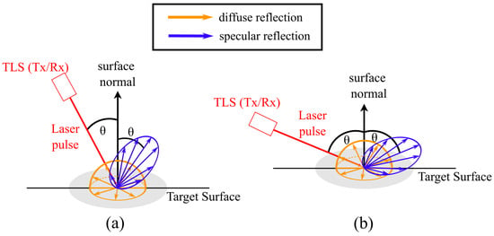
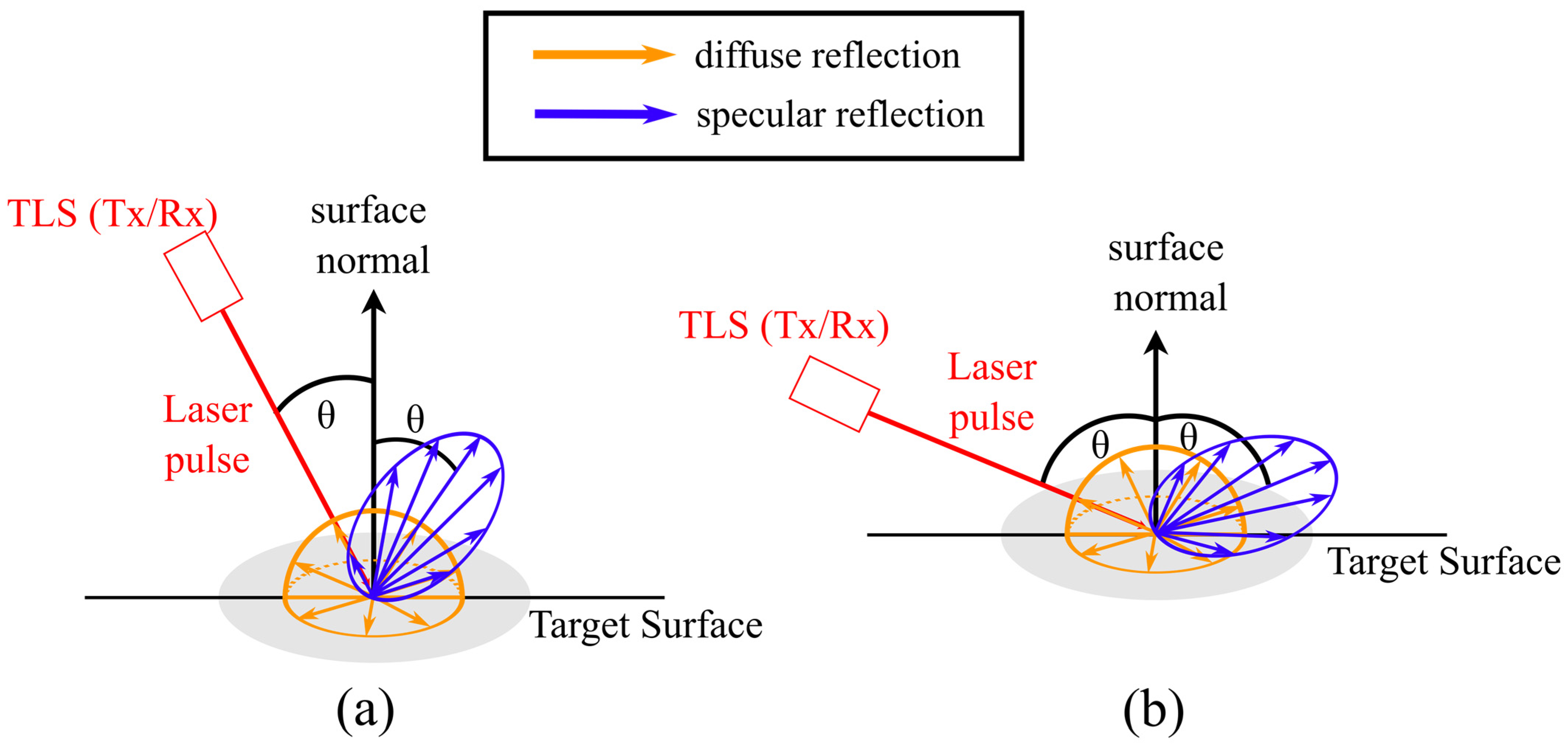
Both diffuse and specular components contribute to the detected TLS intensity, and the contributions of these components vary with the angle of incidence. The contribution of the specular reflection component to the total TLS intensity is greater at a smaller angle of incidence than at a larger angle of incidence [Figure 1a,b]. At large angles of incidence, the specular reflection deviates substantially from the receiver aperture, reducing its contribution to the measured intensity [Figure 1b]. Under such conditions, the diffuse component becomes the dominant contributor to the detected TLS intensity because the scattered energy partially covers the sensor’s field of view regardless of the angle of incidence.

Figure 1. Object reflection at (a) small and (b) large angles of incidence.

TLS intensity is often modeled as a combination of diffuse and specular reflections. Previous studies [2,6,16,18] have proposed the use of Lambert’s cosine law and the Beckmann model to characterize diffuse and specular reflections, respectively, leading to the development of the Lambert–Beckmann (LB) model. The LB model is expressed as follows:

$$I_r^{\prime }=I_0·\left[({1-k}_s)·\mathit{cos}\theta +k_s·{\displaystyle \frac{e^{-\frac{{\mathit{tan}}^2\theta }{m^2}}}{{\mathit{cos}}^5\theta }}\right]$$

(6)

where $\theta$ is the angle of incidence, and $m$ is the surface roughness factor [2,6,27,29]. Smaller $m$ values correspond to increased surface smoothness and greater specular reflection contribution. A higher $k_s$ value also leads to an increase in the contribution of the specular reflection component.

An alternative formulation entails using the Phong model to describe the specular reflection and is suitable for smooth and glossy surfaces [9,15]. The Phong model is expressed as follows [15]:

$$I_r^{\prime }=I_0·\left({(1-k}_s)· \mathit{cos}\theta +k_s·{\mathit{cos}}^{n}2\theta \right)$$

(7)

where $n$ is an exponent that controls the shape and steepness of the specular reflection distribution. Larger $n$ values result in a more abrupt decline in the intensity of specular reflection at small angles of incidence [15].

The contributions of the specular and diffuse reflection components to the total TLS intensity vary with the angle of incidence. Therefore, piecewise models have been used to characterize the variations in TLS intensity in different TLS applications. A previous study [9] used a piecewise model that integrates polynomial approximation to characterize the diffuse component and the Phong model to characterize the specular component [Equation (7)]. This approach is known as the piecewise polynomial Lambert–Phong (PPLP) model [9].

$$I_r^{\prime }=\left\{\begin{array}{c}{I}_0·\left[{\sum }_{i=0}^N{a}_i·{\mathit{cos}}^i\theta +k_s·{\mathit{cos}}^{n}2\theta \right],\theta \le 45°\\ I_0·\left[{\sum }_{i=0}^N{a}_i·{\mathit{cos}}^i\theta \right],\theta >45°\end{array}\right.$$

(8)

In Equation (8), $a_i$ represents the polynomial coefficients, and $N$ represents the polynomial degree. In this study, the $N$ value of the PPLP model was set to 2 in accordance with the methodology used in a previous study [9] to ensure consistency with previous PPLP model implementations. Equation (8) considers both diffuse and specular reflections at small angles of incidence but only diffuse reflection at large angles of incidence [9,15]. However, it is worth noting that the PPLP model uses a fixed transition angle of 45°, which is inherent to the Phong model. This fixed threshold does not account for the considerable morphological diversity observed in natural leaf surfaces.

To allow for flexible transition angles, this study developed a piecewise polynomial LB (PPLB) model, which replaces the Phong model with the Beckmann model for characterizing the specular reflection component. The proposed model is expressed as follows:

$$I_r^{\prime } =\left\{\begin{array}{c}{I}_0·\left[({1-k}_s)·{\sum }_{i=0}^N{a}_i·{\mathit{cos}}^i\theta +k_s·{\displaystyle \frac{e^{- \frac{{\mathit{tan}}^2\theta }{m^2}}}{{\mathit{cos}}^5\theta }}\right],\theta \le {\theta }_T\\ I_0·\left[({1-k}_s)·{\sum }_{i=0}^N{a}_i·{\mathit{cos}}^i\theta \right], \theta >{\theta }_T\end{array}\right.$$

(9)

The PPLB model employs a threshold transition angle ${\theta }_T$ to determine the transition between mixed (diffuse and specular) and purely diffuse reflection regimes. In Equation (9), the polynomial coefficients $a_i$ are shared by the two branches and are fitted as a single set of coefficients, rather than independently for $\theta \le {\theta }_T$ and $\theta >{\theta }_T$. Thus, the polynomial term represents a common diffuse component across both angular regimes, while ${\theta }_T$ controls the angular range over which the Beckmann specular term is included. In this study, ${\theta }_T$ is interpreted as a surface-specific optical boundary associated with the angular range over which the specular reflection contribution remains detectable by the TLS receiver. Because the two branches of the PPLB model are connected at ${\theta }_T$, the fitted intensity response remains continuous across the transition angle. This approach better accounts for the diverse properties of natural leaf surfaces.

2.2. Instrument and Leaf Samples

Leaf samples were scanned using a RIEGL VZ-400 terrestrial laser scanner (RIEGL Laser Measurement Systems GmbH, Horn, Austria) operating at a wavelength of 1550 nm. This system has a ranging accuracy of 5 mm at distances of up to 600 m. Moreover, the scanner conducts automatic intensity calibration to compensate for range-dependent effects. Because the detailed receiver design and optical path of commercial TLS instruments are proprietary, the estimated parameters in this study should be interpreted for the tested sensor-wavelength configuration.

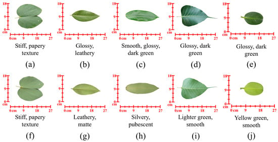
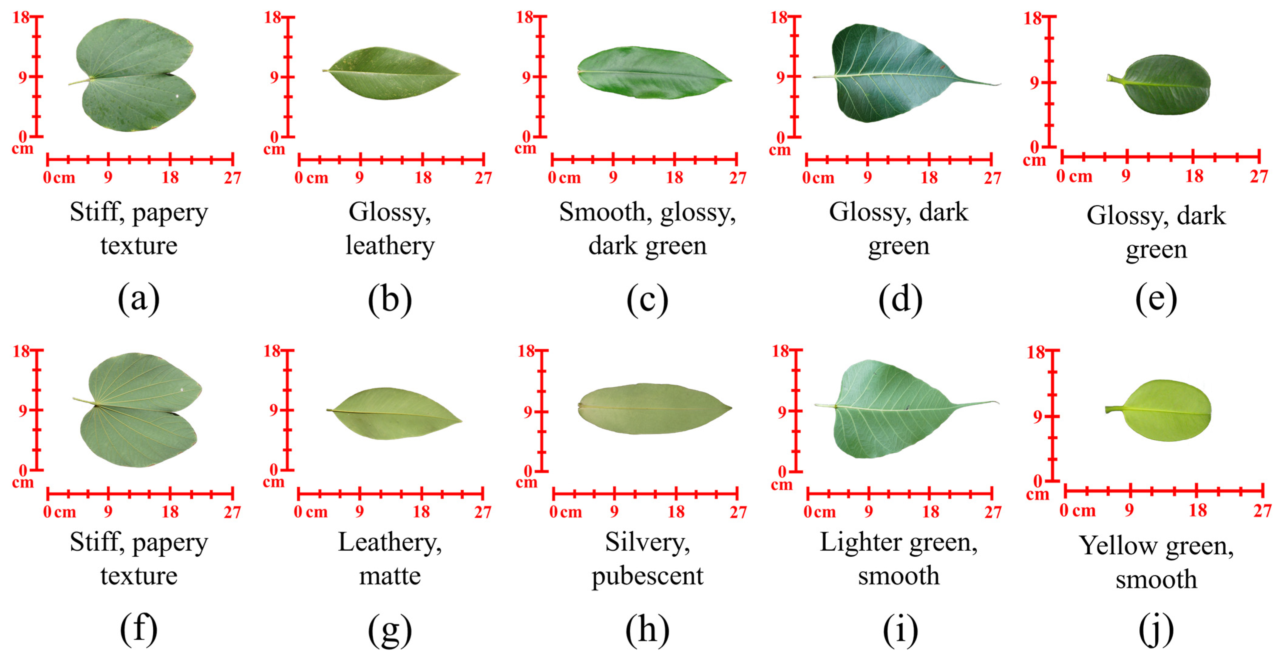
Leaf samples were collected from five tree species within the campus of National Cheng Kung University in Tainan City, Taiwan: the orchid tree (Bauhinia purpurea), golden shower tree (Cassia fistula L.), velvet apple tree (Diospyros discolor), Bodhi tree (Ficus religiosa), and Fukugi tree (Garcinia subelliptica). Eight leaves were collected from each species, resulting in 40 individual leaf samples. For model fitting and presentation, measurements from the eight leaves of the same species and surface side were pooled because preliminary inspection indicated similar angular intensity trends among leaves within each species-surface group. This aggregation was used to characterize species-surface scale responses while still accounting for intraspecies sampling during data acquisition. Representative adaxial and abaxial leaf samples from every species are depicted in Figure 2.

Figure 2. Leaf samples from each species. Adaxial surfaces of leaves from the (a) orchid tree, (b) golden shower tree, (c) velvet apple tree, (d) Bodhi tree, and (e) Fukugi tree. Abaxial surfaces of leaves from the (f) orchid tree, (g) golden shower tree, (h) velvet apple tree, (i) Bodhi tree, and (j) Fukugi tree.

The collected leaves exhibited distinct surface morphologies, ranging from smooth, glossy surfaces (the Bodhi and Fukugi trees) to textured, papery surfaces (the orchid tree) and pubescent structures (abaxial surface of the velvet apple tree) [30]. This diversity ensured that the generalization ability of the developed model could be tested for different surface roughness and specular reflection characteristics.

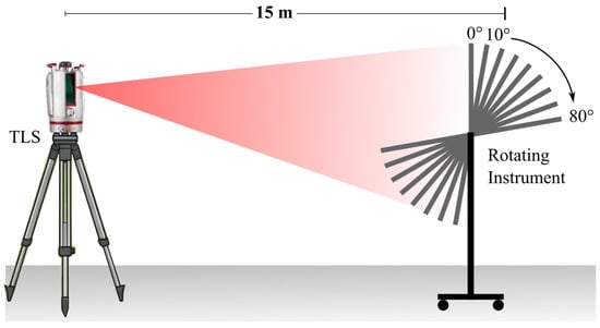
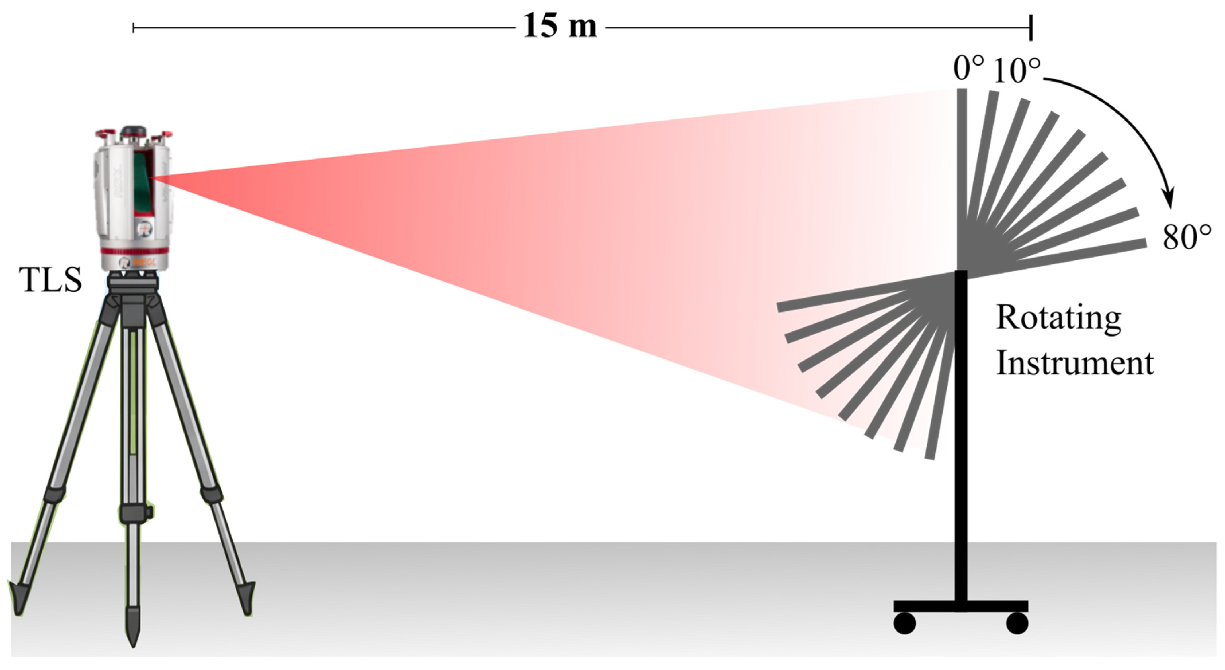
A mounting instrument was placed on a customized rotating platform positioned 15 m from the terrestrial laser scanner (Figure 3). This distance was selected empirically as part of the controlled experimental setup to avoid very close-range measurement conditions while maintaining sufficient point density on the detached leaf samples and stable scanning geometry. Previous TLS intensity correction studies have shown that distance and angle-of-incidence effects influence TLS intensity measurements, highlighting the need for controlled measurement geometry in radiometric experiments [13,23].

Figure 3. Measurement setup for scanning leaf samples.

Individual leaf samples were mounted on the rotating platform, and angular measurements were conducted from 0° to 80° in 10° increments for both adaxial and abaxial surfaces. It should be noted that these values refer to the nominal rotation angles of the mounting platform during data acquisition. The angle of incidence used in the analysis was not assigned directly from the platform rotation angle but was computed point by point from the local leaf surface normal and the incident laser beam direction. All measurements were completed within 20 min of leaf collection as a practical control measure to minimize potential changes in surface condition caused by leaf deterioration. Although minor post-detachment changes, including possible water-loss effects, cannot be fully excluded, the consistent measurement window helped reduce their potential influence across samples.

2.3. Data Preprocessing

2.3.1. Computation of the Angle of Incidence

To calculate the angle of incidence for each measurement point, a local neighborhood was defined around the point by using the k-nearest-neighbors approach. The number of neighbors was set to 30 points to balance local surface representation with computational efficiency. The surface normal vector of each point ($\overrightarrow{N}$) was estimated by fitting a plane to the neighborhood points through principal component analysis. The use of k = 30 provides a balance between local surface representations, but normal estimation may be less stable near leaf edges or in low-density point cloud regions, particularly at large angles of incidence. Therefore, the influence of potentially unstable observations was reduced through the subsequent one standard deviation filtering procedure and by restricting model fitting to the more stable 0–70° angle-of-incidence range. The angle of incidence at each point ($\theta$) was then calculated using the dot product between the incident laser beam vector ($\overrightarrow{L}$) and the normal vector, as expressed in the following equation:

$$\theta ={\mathit{cos}}^{-1}\left({\displaystyle \frac{\overrightarrow{L}·\overrightarrow{N}}{|\overrightarrow{L}||\overrightarrow{N}|}}\right)$$

(10)

2.3.2. Intensity Normalization

The detected raw intensity values were normalized to the maximum instrument-measured intensity to facilitate comparison across different surfaces. The data were organized into angular bins with intervals of 1° based on the point-wise computed angle of incidence, retaining intensity values within one standard deviation of the mean in each bin to reduce the influence of highly scattered observations. The valid point counts and standard deviations of normalized intensity values were summarized by 10° angle of incidence intervals to assess the reliability of the binned observations, particularly in the high angle-of-incidence range (Supplementary Tables S1 and S2). These summaries were used to evaluate data stability together with the one standard deviation filtering procedure; no fixed minimum point count threshold was used as the sole criterion for angular range selection.

Model fitting was performed using the symfit 0.5.6 optimization module in Python 3.10, which implements nonlinear least squares fitting algorithms to obtain the best-fit parameters for each model. For the PPLB model specifically, the piecewise equation was implemented in symfit 0.5.6, and ${\theta }_T$ was treated as an unknown fitted parameter. Therefore, ${\theta }_T$ was optimized together with the other PPLB parameters, including the $k_s$ and $m$. The fitted ${\theta }_T$ value represents the transition angle that best separates the mixed (diffuse and specular) reflection regime from the purely diffuse reflection regime for each species–surface combination.

2.3.3. Selection of the Polynomial Degree

Higher-order polynomial models inherently provide lower fitting errors. However, an excessively high polynomial degree can lead to model overfitting, where the model captures measurement artifacts rather than features that reflect the underlying surface properties. This phenomenon compromises the physical interpretability of surface reflectance models. Therefore, for the PPLB model, the polynomial degree was selected by considering both the reduction in RMSE and the need to maintain a simple and physically interpretable model structure. In this study, polynomial degrees ranging from $N=1$ to $N=5$ were evaluated using the symfit 0.5.6 optimization module in Python 3.10. The final polynomial degree was selected by examining whether increasing $N$ produced a meaningful reduction in RMSE relative to the additional model complexity.

3. Results and Discussion

3.1. Variations in TLS Intensity with Angle of Incidence

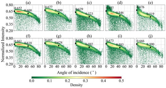
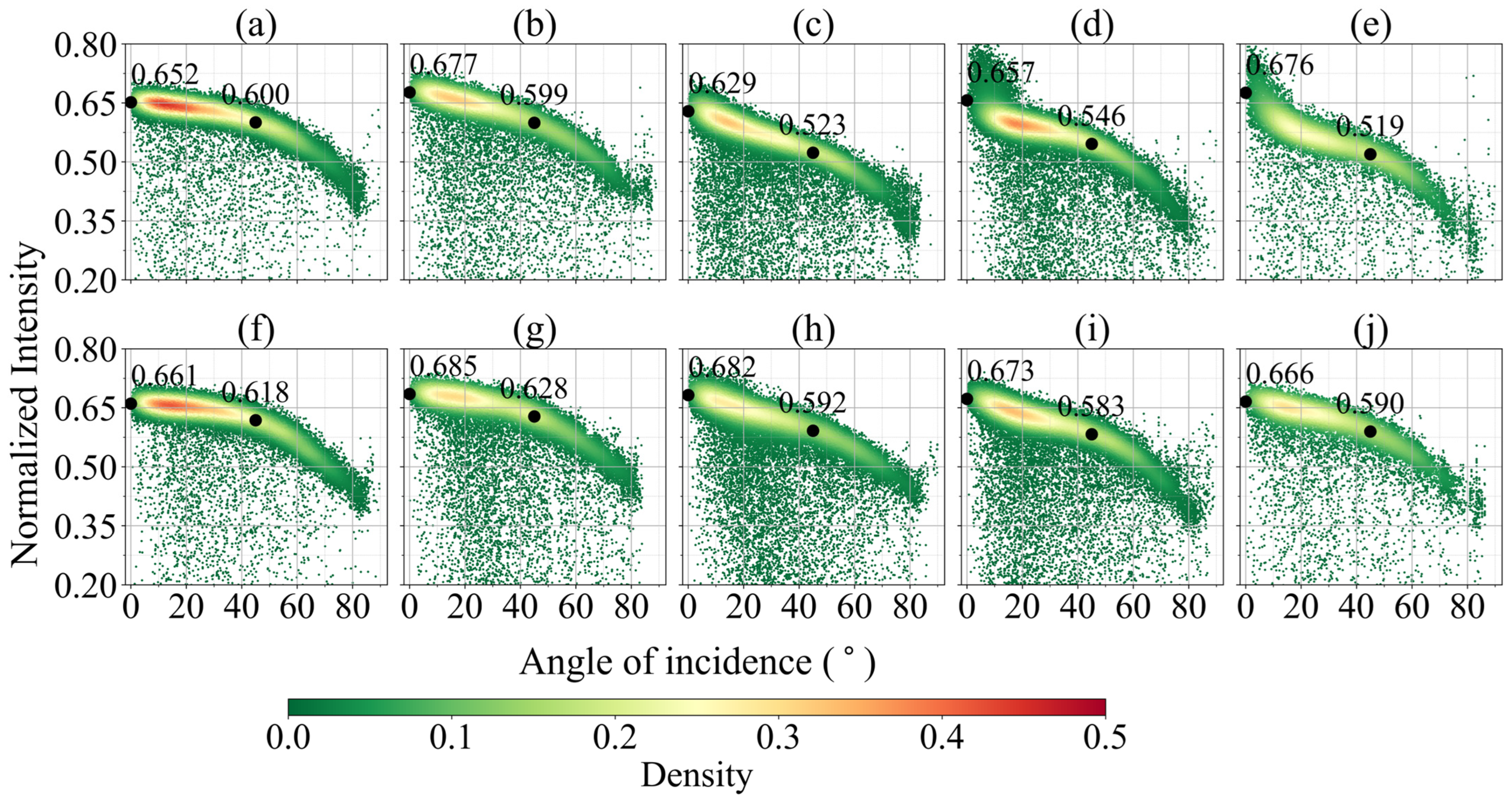
This study analyzed the variations in TLS intensity with the angle of incidence to investigate species- and surface-specific intensity characteristics. Figure 4 illustrates a density plot of the normalized TLS intensity versus the angle of incidence for adaxial and abaxial leaf surfaces across all five species. In this figure, a warmer color represents a higher number of measurements. The figure highlights a curvilinear decrease in TLS intensity with an increase in the angle of incidence. To facilitate the comparison of the intensity values for the adaxial and abaxial surfaces, Figure 4 also presents the median intensity values at angles of incidence of 0° and 45°.

Figure 4. Density plot of normalized TLS intensity versus angle of incidence. Adaxial surfaces of the (a) orchid tree, (b) golden shower tree, (c) velvet apple tree, (d) Bodhi tree, and (e) Fukugi tree. Abaxial surfaces of the (f) orchid tree, (g) golden shower tree, (h) velvet apple tree, (i) Bodhi tree, and (j) Fukugi tree.

For all species and surfaces, the TLS intensity decreased with an increase in the angle of incidence, reflecting the fundamental BRDF behavior. A possible explanation for this finding is that an increase in the angle of incidence caused a higher proportion of the laser signal to be reflected away from the sensor. Moreover, consistent with challenges reported in previous research [2,6], the intensity observations became more dispersed and less clearly concentrated around the main angular trend at angles of incidence greater than 70°. This pattern is also supported by the valid point count and normalized intensity standard deviation summaries in Supplementary Tables S1 and S2, which show decreasing retained point counts and increasing intensity dispersion toward larger angles of incidence. Therefore, model fitting was performed within the 0–70° range to maintain stable parameter estimation across the tested species and surface sides. This condition corresponds to the observations that were scattered under the leaf-surface experimental setup.

Despite the aforementioned common trend, notable variations were observed between species and between leaf surfaces, revealing distinct angular response signatures that reflect the underlying optical surface characteristics. The adaxial surfaces exhibited pronounced species-specific variations, particularly within the range of near-normal angles of incidence (0–30°). Leaves from the orchid tree [Figure 4a] and golden shower tree [Figure 4b] exhibited a gradual decrease in TLS intensity with an increase in the angle of incidence within the near-normal range. By contrast, the Bodhi tree [Figure 4d] and Fukugi tree [Figure 4e] exhibited a sharp decrease in TLS intensity within the aforementioned range. This sharp decrease demonstrates the contribution of specular reflection components at near-normal angles of incidence. The adaxial leaves of the Bodhi and Fukugi trees have smooth surfaces with prominent waxy cuticle layers overlying the palisade mesophyll tissue [31,32]. The adaxial leaves of the velvet apple tree [Figure 4c] showed intermediate characteristics compared to the other species.

Compared with the adaxial surfaces, the abaxial surfaces [Figure 4f–j] showed smaller variations in TLS intensity within the near-normal range of angles of incidence. This result suggests that the contribution of the diffuse reflectance component to the TLS intensity was greater for the abaxial surfaces than for the adaxial ones. Moreover, the abaxial surfaces exhibited a higher normalized intensity than did the adaxial surfaces across all five species. These differences can be attributed to structural variations in leaf anatomy. The adaxial surfaces contained densely packed palisade mesophyll cells, resulting in relatively low backscattered intensities. By contrast, the abaxial surfaces featured loosely arranged spongy mesophyll, which produced relatively high backscattered intensities [31,32].

3.2. Model Fitting Results

3.2.1. Polynomial Degree Selection for the PPLB Model

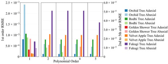
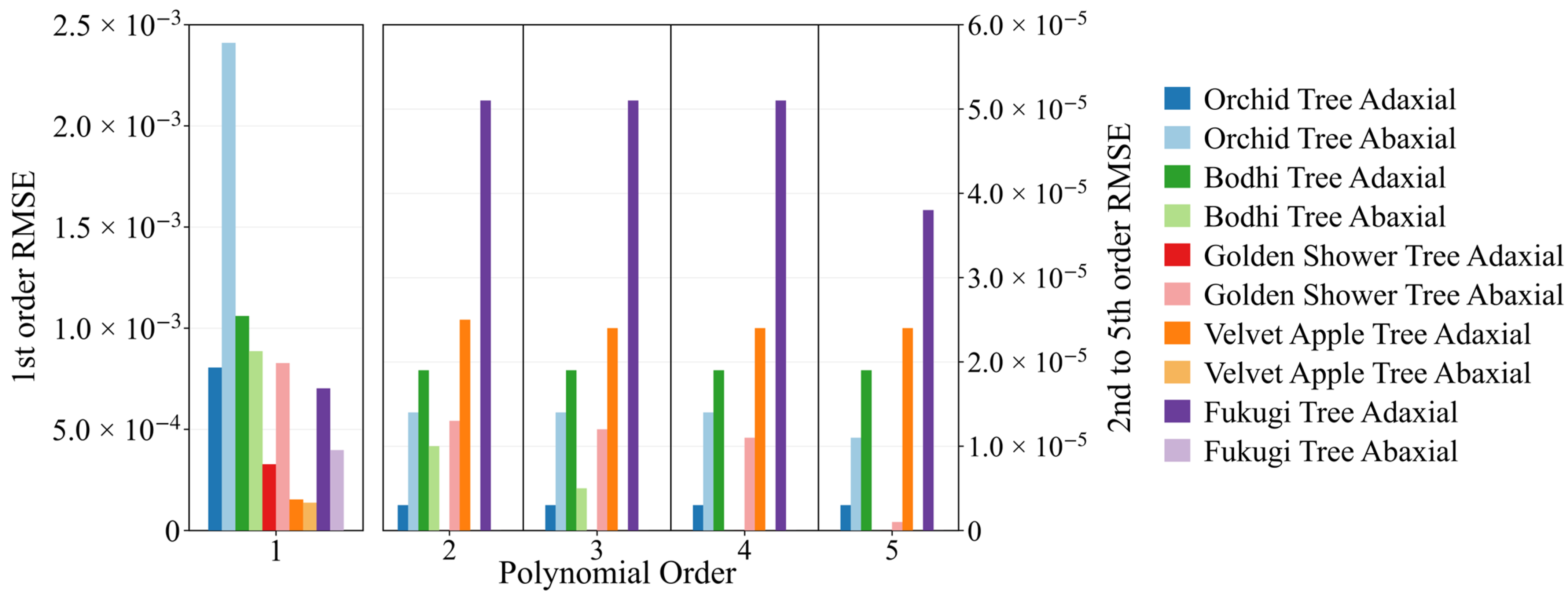
To determine the suitable polynomial degree for the PPLB model, this study evaluated polynomial orders ranging from $N$ = 1 to $N$ = 5 using the symfit 0.5.6 optimization module across the five selected broad-leaved species. Figure 5 displays the RMSE values of the PPLB model for the various polynomial degrees for both adaxial and abaxial leaf surfaces. The RMSE quantifies the fitting errors between the model fitting results and the observed intensity data as a function of angle of incidence.

Figure 5. RMSE values between the fitting results of the piecewise polynomial Lambert–Beckmann (PPLB) model and the observed intensity data for different polynomial degrees ($N$) across all species and leaf surfaces.

When $N$ = 1, the PPLB model becomes equivalent to the LB model. According to Figure 5, the RMSE decreased significantly across all species and both leaf surfaces when $N$ was increased from 1 to 2. Across the ten species-surface combinations, the mean RMSE decreased from $7.704\times {10}^{-4}$ at ($N$ = 1) to $1.35\times {10}^{-5}$ at ($N$ = 2), corresponding to an absolute reduction of $7.569\times {10}^{-4}$. By contrast, increasing the polynomial degree from ($N$ = 2) to ($N$ = 5) reduced the mean RMSE only from $1.35\times {10}^{-5}$ to $9.60\times {10}^{-6}$, corresponding to an additional reduction of $3.90\times {10}^{-6}$. Thus, polynomial terms beyond the second degree contributed marginally to the RMSE in this study. Therefore, second-degree polynomials ($N$ = 2) were selected for subsequent implementations of the PPLB model.

3.2.2. Comparative Model Fitting Results

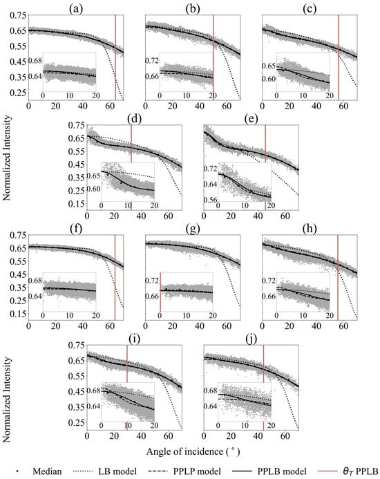
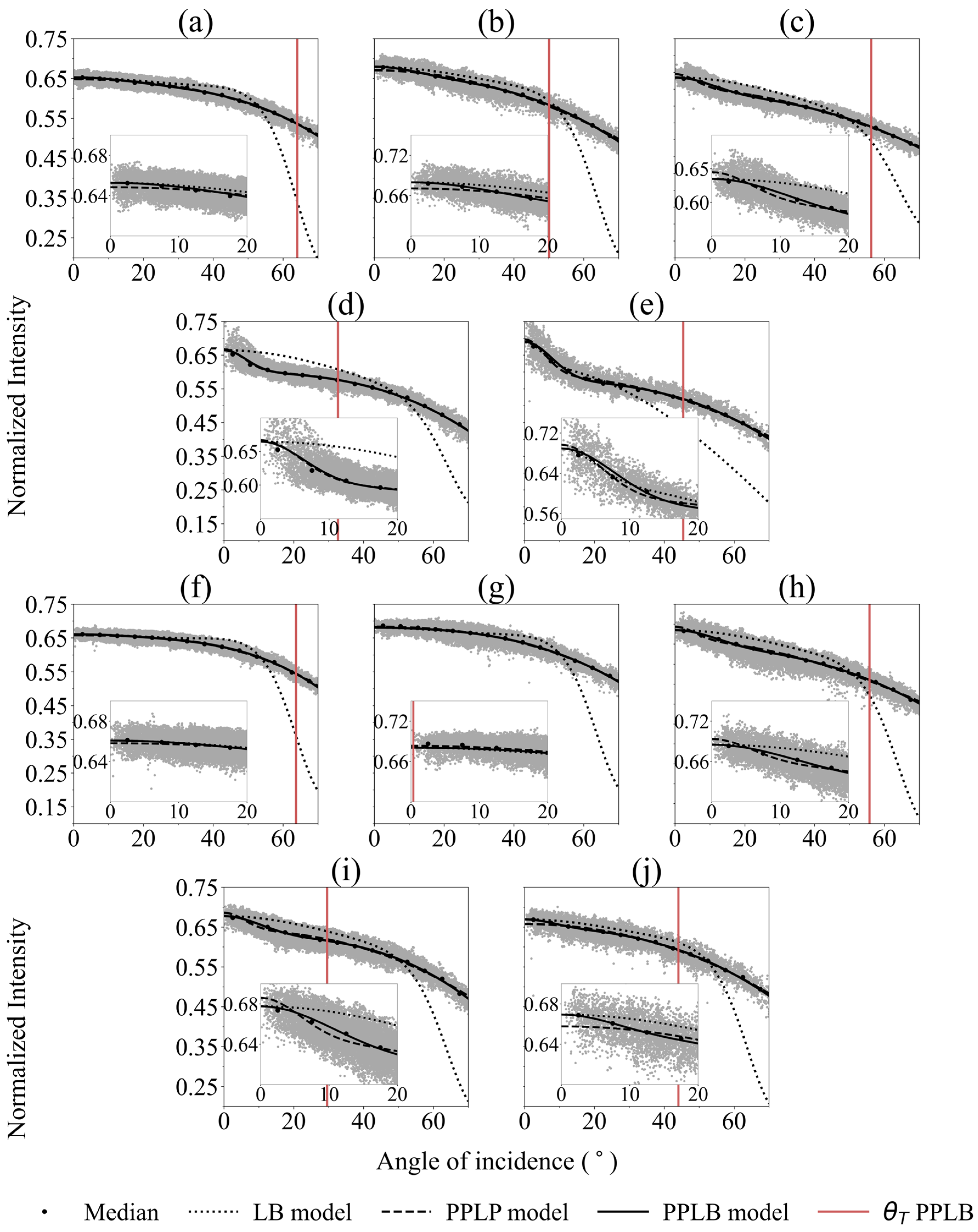
Figure 6 presents a comprehensive comparison of the performance of three BRDF models, namely the LB, PPLP, and PPLB models. The median intensity values (black dots) served as reference baselines to support visual comparison between the observed angular intensity trend and the fitted model curves. The fitting performance of each model was evaluated on the basis of the proximity of its results to these median values, with a smaller deviation indicating a better fit.

Figure 6. Model fitting results for adaxial (a–e) and abaxial (f–j) leaves of the (a,f) orchid tree, (b,g) golden shower tree, (c,h) velvet apple tree, (d,i) Bodhi tree, and (e,j) Fukugi tree.

The fitting results of the LB model showed a close fit to the median intensity values only in specific cases, such as those for the adaxial and abaxial leaf surfaces of the orchid tree [insets of Figure 6a,f], the adaxial leaf surface of the Fukugi tree [inset of Figure 6e], and the abaxial leaf surface of the golden shower tree [inset of Figure 6g]. However, this model showed poor performance at angles of incidence exceeding 50°, indicating its limited capability to represent surface-dependent intensity variations across different leaf types.

Compared with the LB model, the PPLP model demonstrated improved fitting results across angles of incidence, successfully capturing the intensity decline that the LB model failed to capture. However, at near-normal angles of incidence, this model marginally underestimated the TLS intensities for the adaxial leaf surfaces of the orchid tree [inset of Figure 6a] and golden shower tree [inset of Figure 6b] and for the abaxial leaf surfaces of the Fukugi tree [inset of Figure 6j]. These deviations suggest that although the PPLP model captured general TLS intensity trends effectively, it slightly underestimated the specular peak at near-normal angles of incidence.

The PPLB model provided fitted curves that were closely aligned with the observed intensity trends for both adaxial and abaxial leaf surfaces. Notably, it showed good fitting results for the adaxial leaf surfaces of the orchid and golden shower trees [Figure 6a,b], the adaxial and abaxial leaf surfaces of the velvet apple tree [Figure 6c,h], and the abaxial leaf surfaces of the Bodhi and Fukugi trees [Figure 6i,j]. The PPLB model effectively captured both the near-normal specular component and the gradual diffuse transition, indicating its enhanced ability to represent surface-dependent BRDF characteristics.

The red vertical lines in Figure 6 indicate the fitted transition angle (${\theta }_T$) values of the PPLB model. These lines visually mark the angular boundary at which the model transitions from the mixed (diffuse and specular) reflection regime to the purely diffuse reflection regime. For example, the adaxial surface of the Orchid Tree exhibited a relatively large ${\theta }_T$ value of 64° [Figure 6a], indicating that the Beckmann specular component remained active over most of the fitted 0–70° angular range. This behavior differs from the PPLP model, which applies a fixed 45° transition angle regardless of leaf surface type. Therefore, the adaptive ${\theta }_T$ in the PPLB model provides a surface-specific boundary that can better reflect differences in angular intensity behavior among leaf surfaces.

3.2.3. Comparison of the Specular Contributions Estimated by Different Models

According to the previous discussion, the PPLP and PPLB models demonstrated satisfactory fitting results for angles of incidence ranging from 0° to 70°. Consequently, parameter comparisons were performed between these two models. Table 1 presents a summary of the optical parameters estimated by both models for all 10 leaf surfaces. The single parameter set reported in Table 1 therefore represents the pooled species-surface response rather than a single representative leaf. A comparison of specular reflection coefficients indicated that 6 of the 10 surfaces showed similar $k_s$ values in both models. The remaining surfaces (denoted by * in Table 1) exhibited noticeable differences in $k_s$ between the models, where the PPLP model estimated $k_s$ = 0, while the PPLB model estimated a small but nonzero $k_s$.

Table 1. Optical properties estimated by the piecewise polynomial Lambert–Phong (PPLP) and piecewise polynomial Lambert–Beckmann (PPLB). See main text for detailed explanation for *.

Leaf-Sides	Species	PPLB Model				PPLP Model [9]
		${\mathit{k}}_{\mathit{s}}$	m	${\mathit{\theta }}_{\mathit{T}}$ (°)	RMSE	${\mathit{k}}_{\mathit{s}}$	n	RMSE
Adaxial	Orchid tree *	0.022	0.315	64	0.0095	0	25.032	0.0096
	Golden Shower tree *	0.032	0.251	50	0.0128	0	100.164	0.0133
	Velvet Apple tree	0.073	0.234	56	0.0127	0.068	103.456	0.0132
	Bodhi tree	0.096	0.148	33	0.0131	0.099	104.609	0.0131
	Fukugi tree	0.162	0.178	45	0.0183	0.156	103.039	0.0189
Abaxial	Orchid tree *	0.018	0.336	64	0.0096	0	4.638	0.0097
	Golden Shower tree	0	0.545	0	0.0132	0	100.047	0.0132
	Velvet Apple tree	0.057	0.248	56	0.0149	0.050	103.368	0.0152
	Bodhi tree	0.070	0.231	30	0.0133	0.063	103.214	0.0138
	Fukugi tree *	0.028	0.181	44	0.0154	0	3.324	0.0157

The Phong exponent ($n$) in the PPLP model was treated as a mathematical fitting parameter that controls the shape and steepness of the specular term, rather than as a directly interpretable physical property of the leaf surface. The similar high $n$ values obtained for several adaxial and abaxial surfaces, particularly the Golden Shower Tree, Velvet Apple Tree, and Bodhi Tree, indicate that this parameter provided limited discrimination among these leaf surfaces in the present dataset. In this study, physical interpretation focuses primarily on the PPLB parameters $k_s$, $m$, and ${\theta }_T$, while the PPLP model is used as a comparison baseline.

Regarding the surfaces with similar $k_s$ values, both the PPLB and PPLP models captured a pronounced specular contribution for the adaxial leaf surfaces of the Bodhi and Fukugi trees [Figure 6d,e]. The adaxial leaf surface of the Fukugi tree exhibited the highest $k_s$ values among all surfaces (0.162 and 0.156 in the PPLB and PPLP models, respectively) and showed a sharp decrease in the TLS intensity at a near-normal angle of incidence. This result confirms the capability of both models to represent the contribution of specular reflection to the TLS intensity when a sharp decrease in intensity occurs at a near-normal angle of incidence.

For surfaces that exhibited noticeable differences in $k_s$, the PPLP model consistently resulted in a $k_s$ value of 0, whereas the PPLB model identified small but nonzero specular contributions ($k_s$ = 0.018–0.032). These cases demonstrate the ability of the PPLB model to detect small specular reflection contributions that cannot be captured by the PPLP model. Conversely, a $k_s$ value of 0 was obtained for the abaxial leaf surface of the golden shower tree in both models, with ${\theta }_T$ = 0° in the PPLB model. This fitted result indicates that the model did not identify a measurable specular contribution for this surface under the present TLS measurement and fitting configuration. This interpretation is therefore limited to the present model-fitting framework and TLS measurement configuration, and future BRDF measurements would help verify the underlying leaf-surface scattering behavior.

Therefore, compared with the PPLP model, the PPLB model generally produced fitted curves that were more closely aligned with the median intensity values used as the fitting reference. This improved ability of the PPLB model can be attributed to its flexible transition angle (${\theta }_T$). The PPLP and PPLB models are piecewise models that separate a mixed (diffuse and specular) reflection regime from a purely diffuse one; however, the PPLP model employs a fixed transition angle of 45°, which is derived from the Phong model, whereas the PPLB model estimates ${\theta }_T$ directly from the observation data, thereby allowing for adaptive, surface-specific boundary determination. Moreover, the PPLB model may estimate a transition angle close to 45° for some surfaces, such as the Fukugi tree, but it is not constrained to this value and can adapt to other leaf surfaces.

The surface roughness parameter ($m$) provided additional insights into the optical behavior of the leaves. In the original Beckmann formulation, $m$ is commonly related to surface roughness. For leaf surfaces, $m$ can be interpreted as an effective optical roughness parameter derived from the TLS intensity response at 1550 nm. This interpretation extends beyond the apparent external smoothness of the epidermis or cuticle because the measured TLS intensity may also be influenced by subsurface and internal anatomical structures, including mesophyll arrangement and wavelength-dependent scattering within the leaf. Therefore, qualitative visual appearance does not always correspond directly to the fitted $m$ value.

In general, surfaces with higher $k_s$ values tended to have lower $m$ values, indicating stronger specular reflection and smoother effective optical behavior. For example, the adaxial leaf surfaces of the Bodhi and Fukugi trees exhibited the highest $k_s$ values (0.096 and 0.162, respectively) and the lowest $m$ values (0.148 and 0.178, respectively) among the tested surfaces. The adaxial surface of the Velvet Apple Tree showed intermediate angular intensity behavior, but its fitted $m$ value (0.234) was higher than that of the Bodhi Tree (0.148). This difference suggests that the TLS-derived $m$ parameter may also reflect the combined influence of epidermal or cuticle properties, micro-scale surface structure, internal leaf anatomy, and wavelength-dependent interactions. Across all species, the abaxial surfaces consistently showed higher $m$ values than the adaxial ones, indicating that the abaxial surfaces had rougher effective optical behavior and weaker specular reflection.

The ${\theta }_T$ value is a distinctive feature of the PPLB model, defining the angular boundary between mixed (diffuse and specular) and purely diffuse reflection regimes. The tested species exhibited different ${\theta }_T$ values (Table 1). For most species, the adaxial and abaxial surfaces showed similar ${\theta }_T$ values. Specifically, the two leaf surfaces exhibited the same ${\theta }_T$ values for the Orchid Tree (64°) and Velvet Apple Tree (56°) and nearly identical values for the Bodhi Tree (33° vs. 30°) and Fukugi Tree (45° vs. 44°). However, the Golden Shower Tree showed a clear within-species difference, with ${\theta }_T$ = 50° for the adaxial surface and ${\theta }_T$ = 0° for the abaxial surface. This result indicates that the optical transition behavior estimated by the model can differ substantially between the two leaf surfaces within the same species. The ${\theta }_T$ = 0° value should be interpreted as a model-derived fitted response under the present TLS measurement and fitting configuration, indicating that the PPLB model did not identify a measurable mixed (diffuse and specular) regime for this surface. This model-based interpretation represents a limitation of the present study and should be further examined through independent BRDF measurements or additional optical validation in future work. This exception further supports the need for surface-specific transition-angle estimation rather than the use of a fixed transition angle for all leaf surfaces. The PPLB model exhibited RMSE values ranging from 0.0095 to 0.0183, which were comparable to or lower than those obtained using the PPLP model across the tested leaf surfaces (Table 1). These RMSE values are used as fitting-performance indicators to evaluate model behavior under controlled leaf-surface measurement conditions.

Additionally, the results of this study should be interpreted within the experimental scope of the controlled leaf-surface measurements. Although the PPLB model is mathematically applicable to a wider angle-of-incidence domain, the present analysis focused on the 0–70° range because measurements at angles greater than 70° produced sparse and unstable observations under the experimental setup. This condition was mainly associated with the geometric and physical characteristics of leaf surfaces at very large angles of incidence, rather than with the model formulation. The estimated $k_s$, $m$, and ${\theta }_T$ values should also be interpreted for the RIEGL VZ-400 scanner operating at 1550 nm, because TLS intensity may vary with wavelength, beam characteristics, receiver design, and radiometric calibration. Moreover, the five selected broad-leaved species and their adaxial and abaxial surfaces provided diverse surface characteristics for model evaluation, but future studies involving additional species and more extreme leaf morphologies, such as dense hairs, pronounced spots, or highly irregular surface textures, would further support broader application of the proposed model.

4. Conclusions

This study developed a piecewise polynomial Lambert–Beckmann (PPLB) model to improve the characterization of the effect of the angle of incidence on TLS intensity for broad-leaved surfaces. This model incorporates three physically meaningful parameters, namely the specular reflection contribution ($k_s$), surface roughness ($m$), and transition angle threshold (${\theta }_T$). The proposed PPLB model allows ${\theta }_T$ to be estimated from the observed intensity response rather than fixed a priori. Experiments on the adaxial and abaxial surfaces of five tropical tree species showed that a second-order polynomial $(N=2)$ was sufficient to represent the relationship between TLS intensity and angle of incidence within the tested angular range.

The main contribution of the proposed model is not merely a reduction in fitting error, but the demonstration that the transition angle between mixed (diffuse and specular) and purely diffuse reflection regimes varies substantially among natural leaf surfaces. Excluding the case of the Golden Shower Tree abaxial surface, for which ${\theta }_T$ = 0°, the estimated non-zero ${\theta }_T$ values ranged from 30° to 64°. This result indicates that the commonly assumed 45° threshold is suitable for some surfaces, such as Fukugi leaves, but not universal across the tested broad-leaved species. The resulting $k_s$, $m$, and ${\theta }_T$ parameters provide a compact representation of surface-specific TLS intensity behavior and may support future radiometric correction and leaf-surface characterization. The findings should be interpreted within the controlled leaf-surface measurement conditions of this study, including the tested sensor, wavelength, and 0–70° fitting angle-of-incidence range. Further evaluation using additional species, sensors, wavelengths, and field-based canopy measurements would support broader application of the proposed model.

References

- Yan, W.Y.; Shaker, A. Radiometric Correction and Normalization of Airborne LiDAR Intensity Data for Improving Land-Cover Classification. IEEE Trans. Geosci. Remote Sens. 2014, 52, 7658–7673. [Google Scholar] [CrossRef] [Scilit]
- Qian, X.; Yang, J.; Shi, S.; Gong, W.; Du, L.; Chen, B.; Chen, B. Analyzing the Effect of Incident Angle on Echo Intensity Acquired by Hyperspectral Lidar Based on the Lambert-Beckman Model. Opt. Express 2021, 29, 11055. [Google Scholar] [CrossRef] [Scilit] [PubMed]
- Kling, G.J.; Hayden, L.L.; Potts, J.J. UIPlants: Botanic Terminology. Available online: https://woodyplantstutorial.nres.illinois.edu/glossary.asp (accessed on 8 June 2025).
- Brakke, T.W.; Smith, J.A.; Harnden, J.M. Bidirectional Scattering of Light from Tree Leaves. Remote Sens. Environ. 1989, 29, 175–183. [Google Scholar] [CrossRef] [Scilit]
- Jacquemoud, S.; Ustin, S. Leaf Optical Properties; Cambridge University Press: Cambridge, UK, 2019. [Google Scholar]
- Bai, J.; Gao, S.; Niu, Z.; Zhang, C.; Bi, K.; Sun, G.; Huang, Y. A Novel Algorithm for Leaf Incidence Angle Effect Correction of Hyperspectral LiDAR. IEEE Trans. Geosci. Remote Sens. 2022, 60, 5700409. [Google Scholar] [CrossRef] [Scilit]
- Pesci, A.; Teza, G. Terrestrial Laser Scanner and Retro-Reflective Targets: An Experiment for Anomalous Effects Investigation. Int. J. Remote Sens. 2008, 29, 5749–5765. [Google Scholar] [CrossRef] [Scilit]
- Bolkas, D. Terrestrial Laser Scanner Intensity Correction for the Incidence Angle Effect on Surfaces with Different Colours and Sheens. Int. J. Remote Sens. 2019, 40, 7169–7189. [Google Scholar] [CrossRef] [Scilit]
- Tan, K.; Cheng, X. Specular Reflection Effects Elimination in Terrestrial Laser Scanning Intensity Data Using Phong Model. Remote Sens. 2017, 9, 853. [Google Scholar] [CrossRef] [Scilit]
- Tan, K.; Cheng, X. Intensity Data Correction Based on Incidence Angle and Distance for Terrestrial Laser Scanner. J. Appl. Remote Sens. 2015, 9, 094094. [Google Scholar] [CrossRef] [Scilit]
- Tan, K.; Cheng, X. Correction of Incidence Angle and Distance Effects on TLS Intensity Data Based on Reference Targets. Remote Sens. 2016, 8, 251. [Google Scholar] [CrossRef] [Scilit]
- Tan, K.; Liu, K.; Cheng, X. An Empirical Method in Correcting Specular Highlight Phenomenon in TLS Intensity Data. IEEE Access 2016, 4, 9821–9827. [Google Scholar] [CrossRef] [Scilit]
- Kaasalainen, S.; Jaakkola, A.; Kaasalainen, M.; Krooks, A.; Kukko, A. Analysis of Incidence Angle and Distance Effects on Terrestrial Laser Scanner Intensity: Search for Correction Methods. Remote Sens. 2011, 3, 2207–2221. [Google Scholar] [CrossRef] [Scilit]
- Zhu, X.; Wang, T.; Darvishzadeh, R.; Skidmore, A.K.; Niemann, K.O. 3D Leaf Water Content Mapping Using Terrestrial Laser Scanner Backscatter Intensity with Radiometric Correction. ISPRS J. Photogramm. Remote Sens. 2015, 110, 14–23. [Google Scholar] [CrossRef] [Scilit]
- Ding, Q.; Chen, W.; King, B.; Liu, Y.; Liu, G. Combination of Overlap-Driven Adjustment and Phong Model for LiDAR Intensity Correction. ISPRS J. Photogramm. Remote Sens. 2013, 75, 40–47. [Google Scholar] [CrossRef] [Scilit]
- Kaasalainen, S.; Åkerblom, M.; Nevalainen, O.; Hakala, T.; Kaasalainen, M. Uncertainty in Multispectral Lidar Signals Caused by Incidence Angle Effects. Interface Focus 2018, 8, 20170033. [Google Scholar] [CrossRef] [Scilit] [PubMed]
- Phong, B.T. Illumination for Computer Generated Pictures. Commun. ACM 1975, 18, 311–317. [Google Scholar] [CrossRef] [Scilit]
- Kaasalainen, S.; Nevalainen, O.; Hakala, T.; Anttila, K. Incidence Angle Dependency of Leaf Vegetation Indices from Hyperspectral Lidar Measurements. Photogramm. Fernerkund. Geoinf. 2016, 2016, 75–84. [Google Scholar] [CrossRef] [Scilit]
- Hu, P.; Huang, H.; Chen, Y.; Qi, J.; Li, W.; Jiang, C.; Wu, H.; Tian, W.; Hyyppä, J. Analyzing the Angle Effect of Leaf Reflectance Measured by Indoor Hyperspectral Light Detection and Ranging (LiDAR). Remote Sens. 2020, 12, 919. [Google Scholar] [CrossRef] [Scilit]
- Kashani, A.G.; Olsen, M.J.; Parrish, C.E.; Wilson, N. A Review of LIDAR Radiometric Processing: From Ad Hoc Intensity Correction to Rigorous Radiometric Calibration. Sensors 2015, 15, 28099–28128. [Google Scholar] [CrossRef] [Scilit] [PubMed]
- Schill, F.; Holst, C.; Wujanz, D.; Hartmann, J.; Paffenholz, J.-A. Intensity-Based Stochastic Model of Terrestrial Laser Scanners: Methodological Workflow, Empirical Derivation and Practical Benefit. ISPRS Open J. Photogramm. Remote Sens. 2025, 15, 100079. [Google Scholar] [CrossRef] [Scilit]
- Tan, K.; Cheng, X.; Cheng, X. Modeling Hemispherical Reflectance for Natural Surfaces Based on Terrestrial Laser Scanning Backscattered Intensity Data. Opt. Express 2016, 24, 22971. [Google Scholar] [CrossRef] [Scilit] [PubMed]
- Xu, T.; Xu, L.; Yang, B.; Li, X.; Yao, J. Terrestrial Laser Scanning Intensity Correction by Piecewise Fitting and Overlap-Driven Adjustment. Remote Sens. 2017, 9, 1090. [Google Scholar] [CrossRef] [Scilit]
- Tan, K.; Cheng, X. Distance Effect Correction on TLS Intensity Data Using Naturally Homogeneous Targets. IEEE Geosci. Remote Sens. Lett. 2020, 17, 499–503. [Google Scholar] [CrossRef] [Scilit]
- Höfle, B.; Pfeifer, N. Correction of Laser Scanning Intensity Data: Data and Model-Driven Approaches. ISPRS J. Photogramm. Remote Sens. 2007, 62, 415–433. [Google Scholar] [CrossRef] [Scilit]
- Jutzi, B.; Gross, H. Investigations on Surface Reflection Models for Intensity Normalization in Airborne Laser Scanning (ALS) Data. Photogramm. Eng. Remote Sens. 2010, 76, 1051–1060. [Google Scholar] [CrossRef] [Scilit]
- Poullain, E.; Garestier, F.; Bretel, P.; Levoy, F. Modeling of ALS Intensity Behavior as a Function of Incidence Angle for Coastal Zone Surface Study. In Proceedings of the 2012 IEEE International Geoscience and Remote Sensing Symposium; IEEE: New York, NY, USA, 2012; pp. 2849–2852. [Google Scholar]
- Grant, L. Diffuse and Specular Characteristics of Leaf Reflectance. Remote Sens. Environ. 1987, 22, 309–322. [Google Scholar] [CrossRef] [Scilit]
- Poullain, E.; Garestier, F.; Levoy, F.; Bretel, P. Analysis of ALS Intensity Behavior as a Function of the Incidence Angle in Coastal Environments. IEEE J. Sel. Top. Appl. Earth Obs. Remote Sens. 2016, 9, 313–325. [Google Scholar] [CrossRef]
- eFloras Published on the Internet. Available online: http://www.efloras.org/ (accessed on 30 September 2024).
- Ustin, S.L.; Jacquemoud, S. How the Optical Properties of Leaves Modify the Absorption and Scattering of Energy and Enhance Leaf Functionality. In Remote Sensing of Plant Biodiversity; Cavender-Bares, J., Gamon, J.A., Townsend, P.A., Eds.; Springer International Publishing: Cham, Switzerland, 2020; pp. 349–384. ISBN 978-3-030-33157-3. [Google Scholar]
- Xu, K.; Ye, H. Light Scattering in Stacked Mesophyll Cells Results in Similarity Characteristic of Solar Spectral Reflectance and Transmittance of Natural Leaves. Sci. Rep. 2023, 13, 4694. [Google Scholar] [CrossRef] [Scilit] [PubMed]
Disclaimer/Publisher’s Note: The statements, opinions and data contained in all publications are solely those of the individual author(s) and contributor(s) and not of MDPI and/or the editor(s). MDPI and/or the editor(s) disclaim responsibility for any injury to people or property resulting from any ideas, methods, instructions or products referred to in the content. |
© 2026 by the authors. Licensee MDPI, Basel, Switzerland. This article is an open access article distributed under the terms and conditions of the Creative Commons Attribution (CC BY) license.