Comparative Assessment of Low-Cost GNSS Interferometric Reflectometry (GNSS-IR) and Conventional Tide Gauges for Coastal Sea-Level Measurement

Highlights

What are the main findings?

• Low-cost GNSS reflectometry (GNSS-R) measurements strongly agree with conventional tide gauge data, achieving correlations exceeding 85% and centimeter-level accuracy (RMSE of 0.07–0.21 m).
• Statistical analyses across five independent campaigns confirmed no significant difference in the variance of sea-level measurements between the low-cost GNSS-R system and the reference tide gauge.

What are the implications of the main findings?

• Low-cost GNSS receivers and antennas provide a scientifically reliable and economically viable alternative to traditional tide gauges for monitoring coastal sea-level variations.
• The accessibility of this technology enables the expansion of dense coastal monitoring networks, which is critical for tracking climate-driven sea-level changes and improving coastal management.

Abstract

Global climate change drives critical shifts in coastal sea-level dynamics, necessitating the deployment of dense, high-temporal-resolution monitoring networks. To achieve this, GNSS interferometric reflectometry (GNSS-IR) has emerged as a robust technique for monitoring relative sea-level changes. The present study evaluates the performance of a low-cost, multi-band GNSS setup (employing u-blox ZED-F9P receivers) as an economically viable alternative to traditional infrastructure. The GNSS-IR system was installed at the Altata Bay pier (Mexico), and its measurements were validated against a conventional radar tide gauge located 75 m away on the same pier structure. Across five ∼24 h measurement campaigns, the equivalent sea level was retrieved using SNR-based inverse modeling. The low-cost system demonstrated high fidelity, yielding correlations exceeding 85% and RMSE values between 7.0 cm and 21.0 cm. Furthermore, robust statistical validation using the Fisher F-test ($\alpha =0.05$) confirmed no significant differences in measurement variance between the low-cost GNSS-IR system and the reference tide gauge. These findings validate the concept that low-cost GNSS receivers are a scientifically reliable alternative for expanding coastal sea-level monitoring infrastructure.

1. Introduction

Thanks to advances in geodesy, and especially to Global Navigation Satellite Systems (GNSSs), various applications have emerged, such as crustal deformation measurement [1], ionospheric analysis for precursors of seismic activity [2], structural analysis [3], and sea-level monitoring [4]. However, the globally concerning matter of climate change has become one of the most relevant subjects of study, as it is the primary driving factor in global mean sea-level rise [5,6]. Specifically, certain types of phenomena such as the increase in global temperatures lead to anomalous ocean currents, acidification of the ocean waters, melting of polar ice caps, and sea-level rise, among other negative effects [7,8]. Thus, determining sea-level variation is a fundamental part of analyzing climate models to identify the causes of these changes [8], since it affects not only coastal areas but society as a whole. For several decades, conventional tide gauges have been employed to measure sea level and tides using distinct devices, such as gauges based on the traditional rule [9], bubbler systems [10] and radar instrumentation [11].

However, these traditional measurements have certain limitations. Because tide gauges are fixed to the Earth’s surface, they record only relative sea level and are highly susceptible to local vertical land motion (VLM), such as coastal subsidence, making it difficult to separate absolute sea-level rise from crustal deformation [12]. Nonetheless, the scientific community has developed new remote sensing techniques to measure sea level in open ocean and coastal areas, such as satellite radar altimetry [13] and GNSS interferometric reflectometry (GNSS-IR) [14]. While conventional tide gauges remain the standard for millimeter-level accuracy, GNSS-IR serves as a highly capable complementary option, allowing researchers to monitor sea-level variations with centimeter-level precision while expanding spatial coverage in regions where deploying traditional gauges is not feasible.

The remote sensing of sea-level measurements began in recent decades [15]. In June 1990, the European Space Agency (ESA) promoted the use of satellites with pulse-limited altimeters, consolidating the GNSS reflectometry (GNSS-R) method as one of the newest techniques for ocean altimetry implementation in 1993 [16]. Since then, new GNSS-R techniques were developed on the basis of distinct GNSS observations. For example, Reference Soulat et al. [17] proposed sea-level measurements using the phase delay of GPS signals; this approach measures the phase difference between direct and reflected L-band signals, enabling centimeter-level retrieval of surface elevation, sea-surface height, and, in some cases, ocean roughness. The technique requires two antennas to receive and measure the phase difference between the direct signal (RHCP) and the reflected signal (LHCP), usually at the specular reflection point. Later, the same technique was used to monitor the sea level change over a three-month period in Europe [18]. Moreover, Reference Anderson [19] investigated the utility of the signal-to-noise ratio (SNR) from GPS receivers for GNSS-R applications, which was later demonstrated using a specific configuration with a single GPS receiver and antenna [20]. Furthermore, the precision of SNR-based methodologies was improved through forward and inverse modeling of SNR data, which were implemented to estimate snow depth [21,22] and sea level [23,24], respectively.

Similarly, low-cost GNSS receivers have attracted considerable attention within the scientific community and are increasingly being employed in a wide range of geodetic and remote sensing applications.

For example, Reference Ichikawa et al. [25] used a low-cost receiver placed on an unmanned aerial vehicle (UAV) to determine the water level on the shore of Lake Biwa, Japan, from the difference between reflected and direct signals, estimating the geometric height of the UAV using the weighted least squares method, resulting in agreement between the sensor data and the GNSS receiver to 0.01 m accuracy. Moreover, Reference Fagundes et al. [5] evaluated one year of data of SNR data obtained from Lake Guaíba, Brazil, using a low-cost open-source system and compared these data to water-level measurements from a nearby radar tide gauge (located in the same place). The study demonstrated the functionality of the low-cost device, which yielded a 98% coincidence factor and root mean square error (RMSE) of 2.9 cm. Furthermore, a low-cost GNSS buoy was developed to measure sea level in coastal areas where the installation of tide gauges or satellite altimetry is not feasible [26]. The structure, built with tubes and floats, cost approximately £300 and incorporated a single-frequency GNSS receiver configured to record GPS/GLONASS data at 5 Hz. Comparison with a reference tide gauge using the Van de Casteele test [27] showed an RMSE of 1.4 cm, validating its accuracy. The results also revealed high-frequency oscillations associated with coastal geometry and wave action. Likewise, the centimeter-level precision was validated in [28], which used a low-cost GNSS to measure water levels in a mesotidal coastal zone, using the SNR principle to calculate the height difference between the receiver and the water surface. The results were compared to the output of a GNSS tide gauge, resulting in an average daily RMSE of 1.7 cm for a tidal range greater than 3 m. Finally, experiments using low-cost GNSS buoys were also conducted [29]; in that study, four dual-frequency receivers were arranged in a 1.18 m square in Jingye Lake and Bohai Bay (China). The results achieved 0.91 cm (single-frequency) and 0.50 cm (dual-frequency) accuracy, which improved to 0.49 cm and 0.40 cm, respectively, after applying a geometric constraint algorithm. Hence, low-cost GNSS receivers have become a viable and easy-to-deploy tool for diverse geodetic applications.

Although several studies have demonstrated the feasibility of low-cost GNSS-IR systems for sea-level monitoring, most investigations have been conducted under distinct environmental conditions, using different hardware configurations, tidal regimes, and processing strategies. Therefore, the main contribution of this work is the evaluation of a low-cost GNSS-IR architecture under real coastal monitoring conditions in Altata Bay, Mexico. In addition, this study assesses the impact of height-rate and inter-frequency corrections on reflector-height retrievals and validates the resulting sea-level estimates through statistical comparison with an operational tide gauge over five independent measurement campaigns.

To achieve these ends, the present study investigated the performance of low-cost GNSS receivers for sea-level monitoring using two different GNSS-R methodologies. First, five measurement campaigns were conducted to retrieve individual reflected GNSS radio wave signals from the sea at a 1 Hz sampling rate over a ∼24 h period. Second, an equivalent sea-level parameter is computed from the phase difference between the RHCP and LHCP signals as well as the inversion modeling from SNR data.

Finally, the precision was evaluated statistically on the basis of the Fisher “F” hypothesis test and RMSE. The objective of this study is not to investigate long-term tidal constituents or seasonal sea-level variability but rather to evaluate the feasibility and performance of a low-cost GNSS-IR architecture under real coastal monitoring conditions. Altata Bay was selected because it hosts a conventional radar tide gauge operated by the Mexican Navy (SEMAR), located approximately 75 m from the GNSS-IR installation site, enabling direct validation of the retrieved sea-level observations using an independent reference sensor. Furthermore, the measurement campaigns were designed as short-term deployments intended to evaluate hardware performance, data quality, and consistency with tide gauge observations. The campaign durations (17–23 h) were constrained by practical limitations associated with prototype deployment, hardware reliability, power supply stability, and data storage issues encountered during field operations.

The paper is organized as follows: The study area, hardware, software, and methodologies are described in Section 2. In Section 3, the results are described. Lastly, the conclusions are discussed in Section 4.

2. Materials and Methods

2.1. Study Area

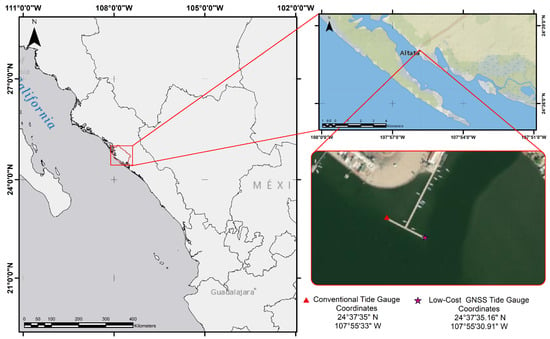
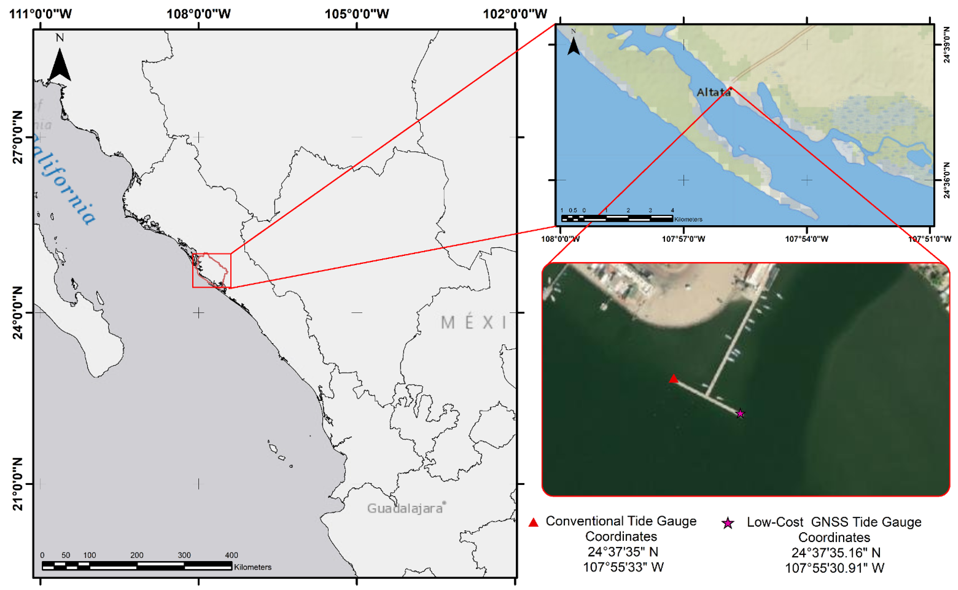
Altata Bay covers an area of 9100 hectares along the continental shelf. It is bordered by the Redo Peninsula and connects to the Pabellón Cove, which is situated along the Lucernilla Peninsula. It is located 62 km from Culiacán Rosales, the capital of the state of Sinaloa, Mexico (see Figure 1). The reference tide gauge station, ALTA043, is located at the geographical coordinates 24°$37\prime 35″\mathrm{N},107°55\prime 33″\mathrm{W}$, with an ellipsoidal elevation of 1 m and installed on a pier 200 m from the coastline. The main sensor is a radar-type device with a 1 min sampling rate operated and administered by the Bureau of the Navy (SEMAR) in Mexico. The tide range varies between 0.35 m and 1.15 m in relation to the mean low water springs (MLWS). The selection of Altata Bay was primarily motivated by the presence of the operational SEMAR radar tide gauge, which enabled a direct comparison between GNSS-IR observations and an independent reference sensor. Furthermore, the proximity between the tide gauge and the GNSS installation site (approximately $75\mathrm{m}$) provided favorable conditions for validating the performance of the proposed low-cost GNSS-IR system under real coastal monitoring conditions.

Figure 1. Study area for this investigation. The reference tide gauge and the low-cost GNSS receiver are represented as a red triangle and a red star, respectively. The distance between the two instruments is 75 m.

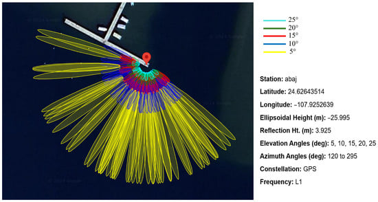
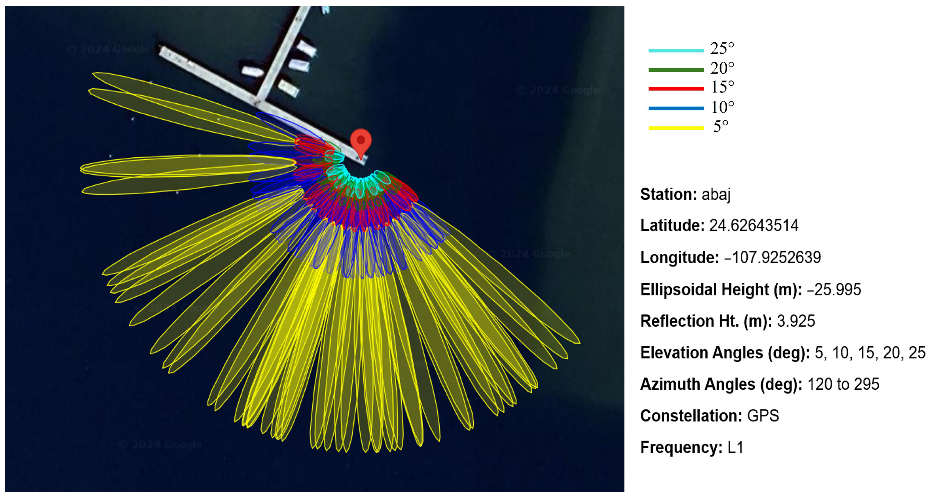
In order to retrieve GNSS signal reflections from the sea, the first Fresnel zones (FFZs) were computed to determine optimal azimuth quadrants and satellite elevation angles. The FFZ, whose formulated components are described in [18], represents the sensing zone where GNSS radio waves are reflected from the surface of interest, in this case, seawater. The FFZ presents size variations and specular points for each satellite elevation angle. Thus, using the FFZ and a visual inspection of site satellite photographs, an azimuth range between 120° and 295° was selected, in conjunction with an elevation angle from 5° to 25° (Figure 2). The latter was calculated using the GPS L1 frequency ($f=1575.42\mathrm{MHz}$, $\lambda =19.05\mathrm{cm}$).

Figure 2. First Fresnel zones (FFZs) for GNSS-R with an antenna height of $3.9\mathrm{m}$ (excluding tidal variations) and fixed elevation angles of $5°$, $10°$, $15°$, and $20°$.

Frequently, it is necessary to perform a quality check (QC) to retrieved SNR observations based on the FFZ. This QC consists of selecting SNR observations with a damped sinusoidal geometry whose amplitude is inversely proportional to the satellite elevation angle, and the quantity of peaks is based on the antenna height over the reflecting surface. This sinusoidal geometry varies when the reflected signal interacts with a surface with distinct physical composition. Therefore, SNR signals with a good-quality sinusoid were used to retrieve sea-level variations. Operating at lower elevation angles (e.g., 5°) elongates the FFZ, increasing the risk of unwanted multipath reflections from nearby moored vessels or the pier infrastructure. To mitigate this, the azimuth mask (120–295°) was strictly defined to orient the sensing footprint toward the open bay, away from the pier. While increasing the minimum elevation cut-off angle to 10° or 15° would reduce the FFZ size and avoid distant obstacles, it would also significantly decrease the number of usable satellite arcs, thereby degrading the temporal resolution of the retrievals. Furthermore, standard quality control (SQC) using the Lomb–Scargle periodogram inherently filters out reflections from static infrastructure, as they fail to produce the distinct, high-amplitude sinusoidal signals characteristic of water reflections.

2.2. Site Installation and Instrumentation

To carry out the hardware installation, a point on the surface of the pier was selected as close as possible to the reference tide gauge. Once the permanent point was defined with geodetic coordinates (latitude: 24°37′35.16″$\mathrm{N}$; longitude: 107°55′30.91″$\mathrm{W}$), it was centered and leveled using a tripod for antenna installation.

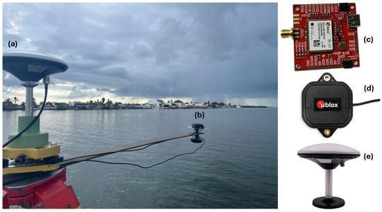
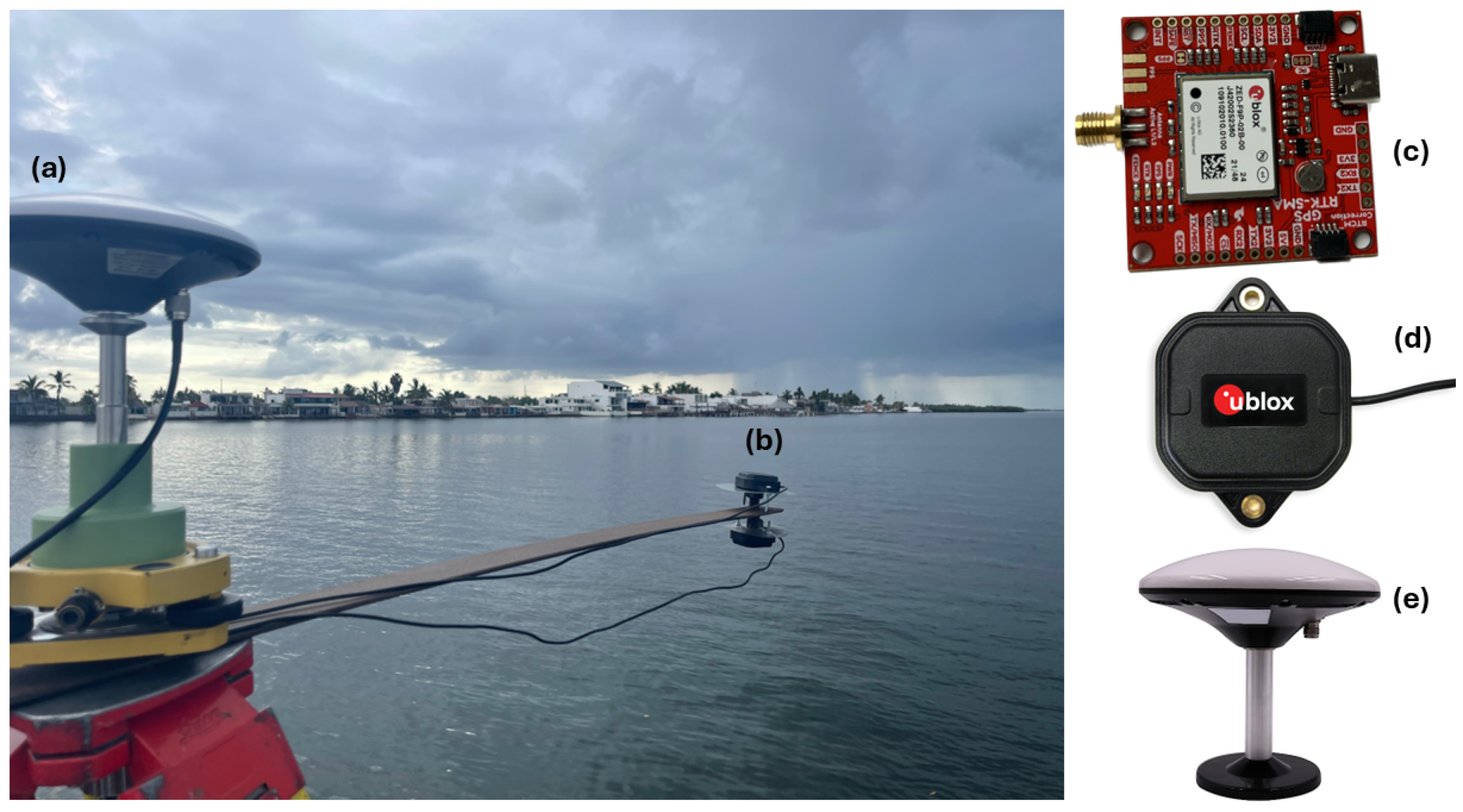
Moreover, a structure was designed using a steel bar that allowed the simultaneous mounting of three antennas during a single observation session. The bar, approximately $100\mathrm{cm}$ long, extends about $50\mathrm{cm}$ into the water (Figure 3).

Figure 3. Installation of three low-cost GNSS receivers and antennas. Experiment A with a single antenna is shown in (a), while experiment B with double antennas is illustrated in (b). The calibrated model BEIBT300 GNSS antenna is shown in (a,e), while the uncalibrated model ANNM00 is illustrated in (b,d).The u-blox ZED-F9P receiver is shown in (c).

Three low-cost GNSS receivers (u-blox ZED-F9P) were used for GNSS data acquisition, each with an approximate cost of $258.7\mathrm{USD}$ (Figure 3c). The ZED-F9P receiver is a compact ($17\times 22\mathrm{mm}$) multi-band low-cost GNSS module providing centimeter-level accuracy through concurrent reception of GPS, GLONASS, Galileo, and BeiDou signals. It features 184 channels and $-167\mathrm{dBm}$ sensitivity and supports RTK positioning. Additionally, it operates within a voltage range of $2.7$–$3.6\mathrm{V}$ and supports USB, UART, SPI, and I²C interfaces, making it suitable for low-power applications. For data processing and identification, the receiver in Experiment A (calibrated, upright) is designated as ABAJ. The two receivers in Experiment B are designated as ARRI (zenith-facing) and BETI (nadir-facing), respectively.

In Experiment A, the topographic point was established directly on the tripod, centered and leveled using conventional methods. This antenna (Figure 3e) was calibrated by the National Geodetic Survey (NGS). In Experiment B, two uncalibrated low-cost antennas (Figure 3d) were mounted at the end of the steel bar to execute the phase delay analysis. One antenna was oriented toward the zenith to capture the direct RHCP signals. The second antenna was mounted facing the nadir. Because standard GNSS antennas are RHCP, physically inverting the antenna towards the surface reverses its polarization frame, making it optimally sensitive to the left-hand circularly polarized (LHCP) signals reflected off the sea surface. Each antenna was connected to an independent u-blox ZED-F9P receiver.

2.3. Data Acquisition and Processing

Five continuous observation campaigns were carried out (Table 1) over periods longer than 12 h, following the considerations in [30]. In this context, GNSS data were acquired using the official u-blox software U-Center [31] with a sampling rate of 1 Hz and an elevation angle mask of 0°. Moreover, an independent “.ubx” file was created for each antenna and later converted to the RINEX v2.11 format using the software RTKLIB 2.4.3 b34 version [32]. It is worth noting that each receiver was preconfigured to log raw GNSS measurements using the built-in RXM-RAWX and RXM-SFRBX messages, ensuring that all necessary observations were recorded in each file for subsequent processing. Although the target duration for each campaign was 24 h to capture complete tidal cycles, the actual recorded durations varied between 17 and 23 h (as detailed in Table 1). These inconsistencies were strictly due to logistical field constraints, primarily unexpected power supply interruptions at the pier and the limited battery lifespan of the data storage systems in the harsh coastal environment. Despite these interruptions, sufficient data was acquired across all campaigns to cover major tidal amplitude shifts, allowing robust statistical comparison. Although the u-blox receivers are multi-band capable, the primary sea-level retrievals were derived from the L1 frequency owing to its higher SNR strength and greater satellite availability, ensuring adequate temporal resolution. The L2C observations were utilized primarily to calculate inter-frequency (IF) biases. As shown in Table 2 and Table 3, incorporating the inter-frequency (IF) corrections in conjunction with the height-rate ($\dot{H}$) correction provided a measurable performance improvement, reducing the overall RMS of the reflector-height time series.

Table 1. GNSS-R measurement campaigns conducted in Altata Bay from October 2023 to January 2024. Time is expressed in local time (LT).

Campaign	Time and Dates		Hours	Sampling Rate (Hz)	Elevation Mask (°)
	Start	End
1	19:00 h 16 October 2023	13:00 h 17 October 2023	18	1	0
2	18:00 h 9 November 2023	17:00 h 10 November 2023	23	1	0
3	18:00 h 23 November 2023	16:00 h 24 November 2023	22	1	0
4	20:00 h 7 December 2023	15:00 h 8 December 2023	19	1	0
5	23:00 h 15 January 2024	16:00 h 16 January 2024	17	1	0

Table 2. Statistics for L1 (1) and L2C (20) frequencies and RMS for each station with and without height-rate correction.

Station	Freq	Bias (m)	Sigma (m)	RMS (no $\dot{\mathit{H}}$) (m)	RMS (w/$\dot{\mathit{H}}$) (m)
Campaign 1
ABAJ	1	0	0.394	0.484	0.482
	20	−0.01	0.424
ARRI	1	0	0.336	0.368	0.351
	20	−0.042	0.287
Campaign 2
ABAJ	1	0	0.493	0.488	0.472
	20	0.128	0.504
ARRI	1	0	0.284	0.325	0.317
	20	−0.054	0.263
BETI	1	0	0.285	0.295	0.292
	20	−0.122	0.269
Campaign 3
ABAJ	1	0	0.197	0.278	0.273
	20	0.025	0.205
ARRI	1	0	0.252	0.274	0.268
	20	−0.054	0.263
BETI	1	0	0.185	0.283	0.276
	20	−0.123	0.209
Campaign 4
ABAJ	1	0	0.153	0.198	0.196
	20	0.086	0.147
ARRI	1	0	0.186	0.214	0.209
	20	−0.041	0.199
BETI	1	0	0.196	0.259	0.254
	20	−0.111	0.191
Campaign 5
ABAJ	1	0	0.215	0.308	0.301
	20	0.26	0.204
ARRI	1	0	0.154	0.286	0.283
	20	0.05	0.169

RMS: root mean square; $\dot{H}$: height-rate correction.

Table 3. RMS per station using the RH + $\dot{H}$/IF correction.

Station	RMS with RH + $\dot{\mathit{H}}$/IF Correction (m)
Campaign 1
ABAJ	0.317
ARRI	0.319
Campaign 2
ABAJ	0.285
ARRI	0.305
BETI	0.285
Campaign 3
ABAJ	0.264
ARRI	0.259
BETI	0.273
Campaign 4
ABAJ	0.187
ARRI	0.203
BETI	0.246
Campaign 5
ABAJ	0.295
ARRI	0.278

RMS: root mean square; RH: reflector height; $\dot{H}$: height-rate correction; IF: interferometric.

We employed the scientific software gnssrefl to retrieve sea-level data from the RINEX files. For further information about the software capabilities and configuration, readers are referred to [33]. The gnssrefl software, an open-source package for GNSS interferometric reflectometry (GNSS-IR), allows the user to compute GNSS-R-based observations for distinct applications such as measuring soil moisture and water level. In the latter, the equivalent sea-level parameters can be computing using different approaches such as phase difference [18] and signal-to-noise ratio (SNR), including the forward and inverse modeling technique [21,23].

2.4. GNSS-R Processing

Generally, the SNR is the main observation involved in ground-based GNSS-R tide gauges. This parameter can record an oscillation in the interference pattern, which is commonly related to the phase difference between the reflected and direct multipath signals. Therefore, using this data in the gnssrefl software, we computed water-level variations based on the phase-delay method and applied a forward and inverse model for SNR observations.

2.4.1. SNR Inverse Modeling (Experiment A)

In this two-step methodology, the forward model represents the SNR observations as the ratio between the noise power $P_n$ and the signal power $P_s$. The latter can be described as a function of direct and reflected powers ($P_d$ and $P_r$, respectively) and phases (${\varphi }_d$, ${\varphi }_r$, respectively). The trend and detrended interference fringes can be decomposed as

$$\mathrm{tSNR}={\displaystyle \frac{P_d+P_r}{P_n}}$$

(1)

$$\mathrm{dSNR}={\displaystyle \frac{2\sqrt{P_d}\sqrt{P_r}cos\left({\varphi }_i\right)}{P_n}}$$

(2)

where ${\varphi }_i$ is the interferometric phase, defined as the difference between the direct and reflected phases.

Consequently, the interferometric phase can be approximated as

$${\varphi }_i\approx {\displaystyle \frac{4\pi Hsine}{\lambda }}$$

(3)

where H is the reflector height above the reflecting surface and $\lambda$ is the carrier wavelength.

Thus, the SNR model can be expanded considering imperfections in the physical parameters as follows [21]:

$$\mathrm{SNR}=\left(1+P_i^{\prime }+2\sqrt{P_i^{\prime }}cos\left({\varphi }_i^{\prime }\right)\right){\displaystyle \frac{P_d^{\prime }}{P_n}}$$

(4)

where $P_i^{\prime }$ is the ratio between the interferometric power $P_i$ and the complex bias term $B=\left|B\right|exp\left(i{\varphi }_B\right)$, respectively. ${\varphi }_i^{\prime }$ is the difference between the interferometric phase and the interferometric bias.

$P_d^{\prime }$ is the ratio between the direct power and the noise power bias, defined as $K={10}^{K_{dB}/10}$, where $K_{dB}$ can be expanded as a polynomial function of the sine of the elevation angle. Because the sea surface is continuously varying, the reflector height rate ($\dot{H}$) and the elevation angle rate ($\dot{e}$) are estimated iteratively using a polynomial spline fitting approach. In this study, the iterative process was considered to have converged when the change in the estimated height correction between successive iterations was less than $0.001\mathrm{m}$ (1 mm). On average, stable convergence was achieved within 3 to 4 iterations across the measurement campaigns. Once convergence was reached, these corrections were applied to the initial observations.

Furthermore, the polynomial coefficient phase bias ${\varphi }_B^{\left(1\right)}$, derived from the reflection phase bias ${\varphi }_B$, can be adjusted to an equivalent reflector height bias as

$$H_B={\displaystyle \frac{{\varphi }_B^{\left(1\right)}}{4\pi }}$$

(5)

Hence, the reflector height can be calculated as

$$H=H_A-H_B$$

(6)

where $H_A$ is an a priori first-guess value and $H_B$ is the a posteriori bias estimate. In this study, $H_A$ was obtained from the initial SNR-based reflector-height retrieval using the selected azimuth and elevation masks. This first-guess value was derived from the dominant oscillation frequency of the detrended SNR arcs. Subsequently, $H_B$ was estimated during the inverse modeling procedure as the equivalent reflector-height bias associated with the phase-bias term. Thus, the final reflector height was computed as $H=H_A-H_B$.

Later, the inverse model incorporated the forward model using a non-linear least squares procedure. The resulting parameter corresponds to the vertical distance from the antenna phase center to the reflecting surface.

Finally, we computed the initial reflector height (RH) based on the GPS constellation, considering the azimuth and elevation masks, eliminating outliers and applying a spline-based sinusoidal adjustment. Subsequently, RH corrections (height/time correction) were applied to re-estimate RH. Furthermore, the inter-frequency (IF) bias between L1 and L2C observations was estimated by calculating the mean difference between the simultaneous height retrievals of the two frequencies over a moving time window. This constant offset was then subtracted from the L2C retrievals to align them with the L1 reference height.

The correction workflow was implemented sequentially. First, the initial reflector height (RH) was estimated from the dominant oscillation frequency of the detrended SNR arcs using the selected azimuth and elevation masks. Then, the height-rate correction (RH + $\dot{H}$) was applied iteratively to account for the temporal variation of the reflecting sea surface during each satellite arc. Finally, the inter-frequency (IF) bias estimated from the L1 and L2C reflector-height solutions was removed from the solution, and the reflector heights were recomputed to obtain the final RH + $\dot{H}$/IF estimates. This procedure allowed the evaluation of the RMS reduction associated with each correction stage.

According to [20], for a moving flat surface with tidal variations greater than $7\mathrm{m}$ over a 24 h period, the SNR model for flat surfaces ($d=2Hsine$) does not satisfy the solution. This is because GPS measures the distance between the antenna and the reflecting surface, and therefore the frequencies of the reflected signals are not correlated with the measurements obtained by a tide gauge.

Therefore, for moving/time-varying flat surfaces, the correction is as follows [34]:

$$\Delta H_R=\dot{H}tane{\dot{e}}^{-1}$$

(7)

where $\Delta H_R$ is the height correction, while $\dot{H}$ and $\dot{e}$ are the temporal rates (time derivatives) of the reflecting surface height and the satellite elevation angle, respectively.

Assuming the surface is locally constant, the values of $\dot{H}$ and $\dot{e}$ are obtained iteratively. Once the corrections are computed, they are applied to the initial observations to obtain the updated sea level (RH) for each station in each measurement campaign.

2.4.2. Phase Delay Analysis (Experiment B)

The phase delay analysis method employs two antennas and two receivers; one antenna points towards the zenith (RHCP) and records the direct GNSS signals coming from the satellite, while the second antenna is oriented towards the nadir (LHCP) and records the signals reflected on the sea surface, which present a phase delay [35]. Consequently, since the reflected signals show an increase in the path length traveled, the nadir-oriented antenna will appear as a virtual antenna located below the surface; therefore, the distance between the virtual antenna and the sea surface will be equal to the distance between the sea surface and the actual LHCP antenna. Thus, it can be deduced that as the sea level changes, the path length of the reflected signals also changes, making the LHCP antenna appear to change its vertical position. Hence, the height of the sea surface is directly proportional to the height of the LHCP antenna above the surface ($h_a$); therefore, the vertical relationship between the two antennas ($\Delta v$) (RHCP–LHCP) and the parameter $h_a$ is expressed by the following geometry:

$$\Delta v=2h_a+d$$

(8)

where d is the vertical distance between the antenna phase centers. On the basis of [35], one of the main forms of phase delay analysis is through the GNSS phase observation:

$${\lambda }_i{\Phi }_A^j={\rho }_A^j+c({\tau }_A-{\tau }^j)+Z_A^j-I_A^j+{\lambda }_i{N}_A^j$$

(9)

where ${\lambda }_i$ is the wavelength of the GNSS carrier signal, ${\Phi }_A^j$ is the carrier phase in complete cycles, ${\rho }_A^j$ is the satellite geometric range, c is the speed of light in a vacuum, ${\tau }_A$ is the receiver clock bias, ${\tau }^j$ is the satellite clock bias, $Z_A^j$ is the tropospheric delay, $I_A^j$ is the ionospheric delay, and $N_A^j$ is the phase ambiguity.

Moreover, the formulation for the single-time difference phase considering two receivers, denoted as A and B, both observing the same satellite j, can be inferred from Equation (10) as

$${\lambda }_i\Delta {\Phi }_{A,B}^j=\Delta {\rho }_{A,B}^j+c\Delta {\tau }_{A,B}+\Delta Z_{A,B}^j-\Delta I_{A,B}^j+{\lambda }_i\Delta N_{A,B}^j$$

(10)

where $\Delta$ denotes the difference between the two receivers. Consequently, the relative clock bias ($\Delta {\tau }_{A,B}$) between the two independent receivers in the single-difference phase equations, was estimated as an independent epochwise white-noise parameter during the non-linear least squares adjustment using RTKLIB. Alternatively, this term is completely eliminated when forming double differences if a reference satellite is utilized. Therefore, when considering differences with respect to the same satellite, the clock bias term becomes negligible. In addition, the ionospheric effects $\Delta I_{A,B}^j$ and tropospheric effects $\Delta Z_{A,B}^j$ are not considered due to the short distance between the two antennas.

Hence, the geometric difference on a short baseline can be expressed in a local coordinate system [35], as a function of the satellite azimuth ($\alpha$) and elevation angle ($\theta$), yielding

$$\Delta {\rho }_{A,B}^j=\Delta esin\left({\alpha }^j\right)cos\left({\theta }^j\right)+\Delta ncos\left({\alpha }^j\right)cos\left({\theta }^j\right)+\Delta vsin\left({\theta }^j\right)$$

(11)

where $\Delta e$, $\Delta n$, and $\Delta v$ are the east, north, and vertical components of the baseline, respectively. If the horizontal baseline is known, it can be neglected, allowing the east and north components to be excluded in order to reduce the number of unknowns.

2.5. Statistical Approach

To determine whether the variations or differences are significant with respect to the tidal trend, the Fisher statistical test was selected. This test relates the variances of the observations, allowing a comparison of the proportion of variances between two data sets as follows [36]:

$$H_0:{\displaystyle \frac{S_1^2}{S_2^2}}=1$$

(12)

$$H_a:{\displaystyle \frac{S_1^2}{S_2^2}}\ne 1$$

(13)

where $H_0$ and $H_a$ are the null and alternative hypotheses, respectively; $S_1^2$ and $S_2^2$ are the variances of the two datasets to be compared, where the statistical test is applied for each station in each observation campaign. Therefore, the null hypothesis is accepted if

$$F_i<F_{\alpha /2,v_{1i},v_{2i}}$$

(14)

where $F_i$ is the statistical value for each station, while $F_{\alpha /2,v_{1i},v_{2i}}$ is the critical F-value corresponding to the upper tail area $\alpha /2$, with $v_{1i}$ and $v_{2i}$ degrees of freedom in the numerator and denominator, respectively, obtained from the Fisher distribution. The significance level is $\alpha =0.05$.

Finally, the 95% confidence intervals (CIs) are established [36]:

$${\displaystyle \frac{1}{F_{\alpha /2,v_{1i},v_{2i}}}}·{\displaystyle \frac{S_1^2}{S_2^2}}<{\displaystyle \frac{{\sigma }_1^2}{{\sigma }_2^2}}<{\displaystyle \frac{S_1^2}{S_2^2}}·F_{\alpha /2,v_{1i},v_{2i}}$$

(15)

where ${\sigma }_1^2/{\sigma }_2^2=1$ under the null hypothesis.

3. Results

When evaluating the performance of both experiments, temporal resolution is a critical factor. The reference radar tide gauge operates continuously, yielding a resolution of 1 to 5 min. In Experiment A (SNR inverse modeling), the temporal resolution is dictated by the passage of satellites through the FFZ. Using only the GPS constellation, this resulted in approximately 15 to 20 height retrievals per day per frequency (L1/L2C). When fused, the SNR method provided a temporal resolution of roughly one measurement every 30 to 45 min. Conversely, Experiment B (phase-delay method) compares the continuous carrier-phase measurements between the zenith and nadir antennas. This allowed epoch-by-epoch tracking, yielding a high temporal resolution of 1 Hz (1 s), which was subsequently reduced to 5 min to match the reference tide gauge sampling rate for statistical comparison.

Furthermore, Table 2 summarizes the RMS values and inter-frequency (IF) biases obtained from the initial L1 and L2C reflector-height retrievals before and after the application of the RH + $\dot{H}$ correction. Subsequently, Table 3 reports the RMS values after the IF biases have been removed from the solution and the reflector heights have been using the RH + $\dot{H}$/IF correction. Thus, Table 2 evaluates the effect of the height-rate correction, whereas Table 3 presents the final RMS values after the application of both the height-rate and inter-frequency corrections.

It is critical to note that a physical geodetic leveling survey was not conducted to tie the GNSS-IR antenna phase centers to the tide gauge benchmark. Because the objective of this study is to evaluate the dynamic tracking capability of the low-cost sensors (i.e., amplitude, variance, and correlation), the datum alignment was performed purely numerically. Relative sea-level time series were created by subtracting the respective mean water level from each instrument’s dataset (mean centering). Consequently, the calculated offsets evaluate the relative phase and amplitude tracking between the sensors, rather than absolute geodetic water levels. The vertical datum between the tide gauge and GNSS-R is based in a distinct type of representation. Although an offset may be used to link the TG to a benchmark network, the initial tide gauge measurements represent the separation between the sensor’s internal origin and sea level. Likewise, the distance between the antenna phase center and the reflective surface is represented by GNSS-R retrievals, which, if needed, can be further linked to the earth’s ellipsoid by GNSS positioning. Therefore, the vertical origin of the tide gauge and the GNSS-R sea-level measurements were shifted in order to compare the sea level changes between the proposed sensors. Thus, relative sea levels were created by deducting the mean sea level from each instrument’s time data. Furthermore, the tide gauge observations were interpolated to match the GNSS-R observation sample.

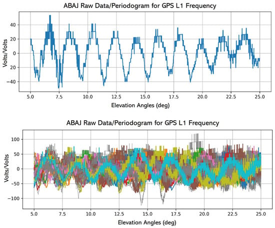
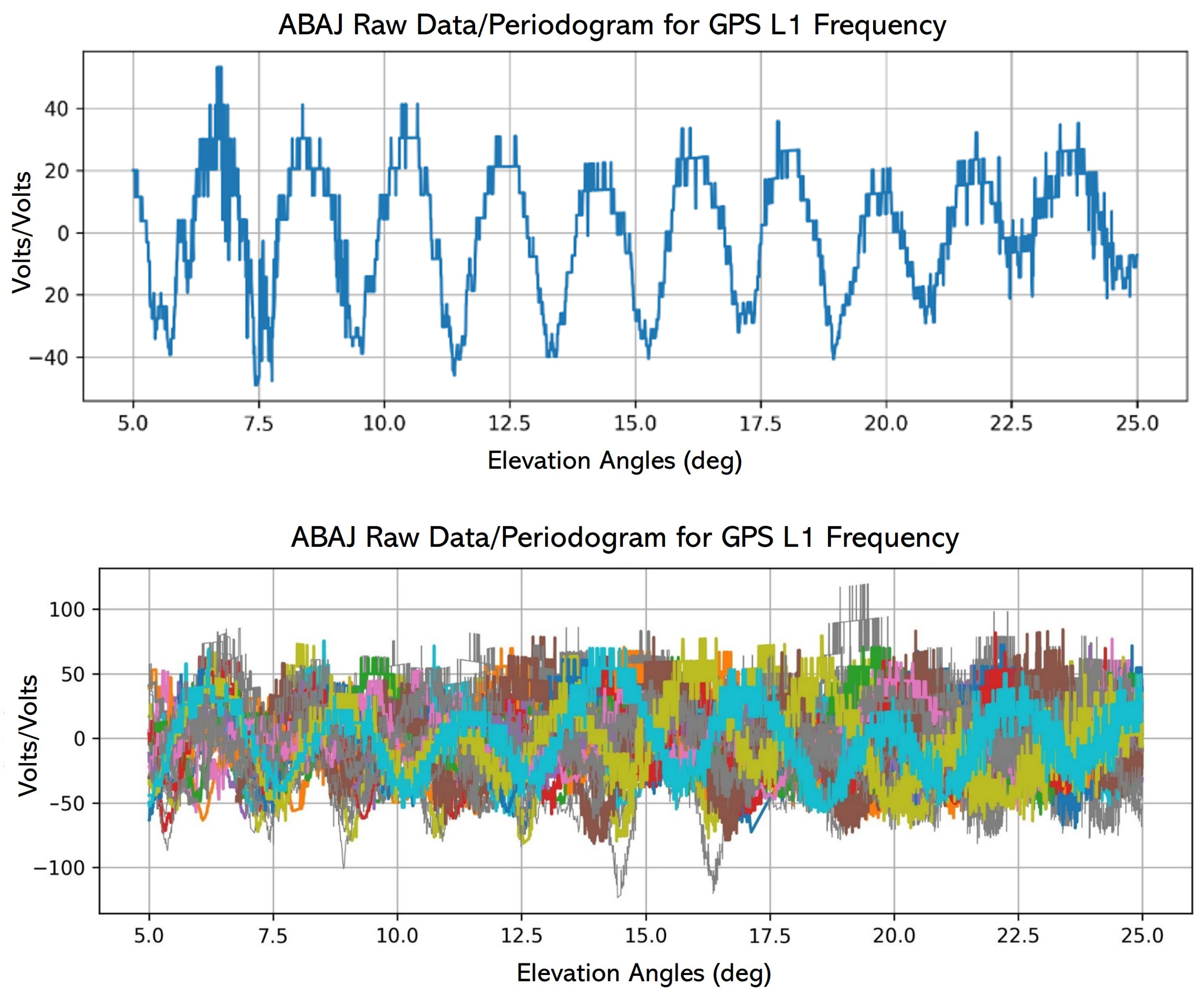
However, when working with spectral analysis techniques such as the Lomb–Scargle periodogram (LSP), it is necessary to remove the effect of the direct GNSS signal using a low-order polynomial and to convert the signal power from dB-Hz to linear units (volts/volts), since the LSP estimates the spectral power by fitting sinusoidal functions at different frequencies to the data. Therefore, we detrended the SNR observations from the five campaigns prior to the LSP analysis (Figure 4).

Figure 4. The (top) panel shows the detrended GPS-L1 SNR measurements from the GNSS-R station ABAJ. The observations correspond to mean-removed and low-order polynomial detrended SNR data represented as a function of satellite elevation angle, rather than raw SNR measurements. Each colored curve represents the continuous track of an individual satellite (differentiated by PRN) over the local sky. The (bottom) panel represents one satellite arc from DOY 314 with an azimuth of 150°.

Thereafter, we used the GNSSREFL software, which extracts SNR data from the GPS frequencies L1, L2C, and L5 (if available) and saves it to a new file with “.snr66” extension (for angles less than 30°). Subsequently, the resulting SNR data were analyzed to estimate the height of the reflecting surface (RH) including the RH corrections for higher amplitudes. Table 2 shows the statistics for the GPS constellation L1 and L2C frequencies denoted in the code as 1 and 20, respectively. Furthermore, the inter-frequency (IF) biases and the RMS values for the initial observations, with and without the RH + $\dot{H}$ correction, can be observed. Moreover, bias is computed as the mean vertical deviation of the frequency-specific retrievals, and sigma ($\sigma$) represents the standard deviation of these retrievals. To compute the final station RMS, the L1 and L2C retrievals were fused into a single time series after correction for the IF bias, thereby increasing data density and improving the overall robustness of the height estimation.

Additionally, the inter-frequency (IF) biases were removed from the solution, and the reflector heights were recomputed using the RH + $\dot{H}$/IF correction, yielding the RMS values presented in Table 3.

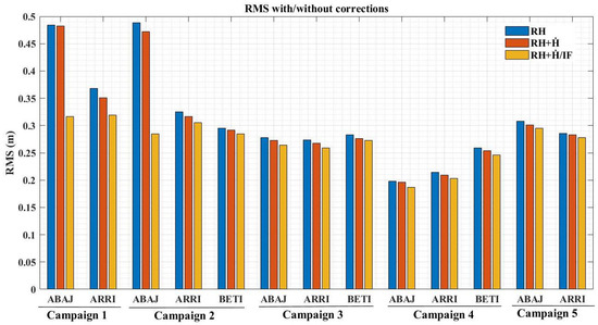
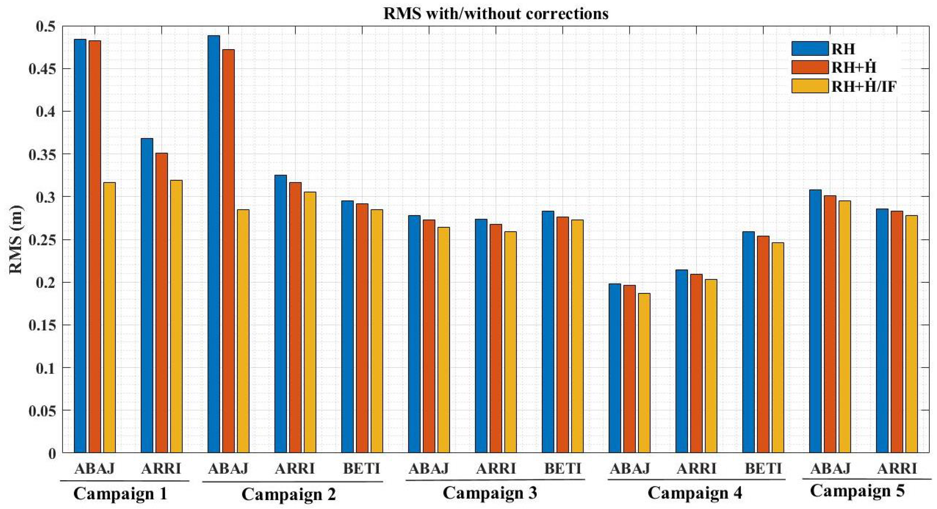
In this sense, we computed the root mean square (RMS) differences for each station in each campaign (Figure 5). The RMS values of the initial height estimates generally ranged between 0.198 m and 0.488 m. For campaign one (C-1), an initial RMS of 0.484 m and 0.351 m was recorded for stations ABAJ and ARRI, respectively. A significant improvement was obtained after applying the RH + $\dot{H}$/IF corrections, with an RMS of 0.317 m for ABAJ and 0.319 m for ARRI, indicating the variability of the data with respect to the best-fit line. For subsequent campaigns, a relatively large initial RMS (0.488 m) was observed at station ABAJ in campaign 2 (C-2). This improved considerably after the application of the height-rate and inter-frequency corrections, resulting in an RMS of 0.285 m. The best fit was obtained at station ABAJ in the fourth (C-4), with an uncorrected RMS value of 0.198 m and an RMS of 0.187 m once the corrections were applied.

Figure 5. Root mean square (RMS) of the estimated reflector heights per station. RH: initial estimate; RH + $\dot{H}$: height-rate corrected estimate; RH + $\dot{H}$/IF: estimate corrected for both height-rate and inter-frequency effects.

Moreover, the accuracies obtained from the sinusoidal adjustment are relatively high; however, to evaluate the performance of the instruments, it is necessary to compare the data obtained (final heights) after adjustment with the data derived from a conventional tide gauge (TG). For this purpose, all measurements were compared, i.e., per station/campaign, over the same time period (GPS), to observe whether they followed the tidal trends observed by the TG. Consequently, we performed a correlation analysis between the two heights (GNSS and tide gauge) (Table 4).

Table 4. Statistics comparing GNSS and tide gauge heights per campaign.

Station	Correlation ($\mathit{\rho }$)	RMSE (m)	Campaign
RH-ABAJ	0.85	0.17	1
RH-ARRI	0.83	0.18
ABAJ	0.97	0.07	2
ARRI	0.90	0.13
BETI	0.96	0.08
ABAJ	0.95	0.08	3
ARRI	0.91	0.11
BETI	0.92	0.10
ABAJ	0.80	0.11	4
ARRI	0.61	0.21
BETI	0.65	0.19
ABAJ	0.96	0.08	5
ARRI	0.93	0.10

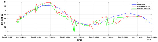
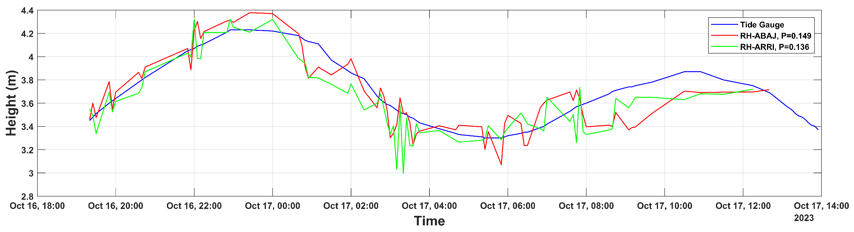
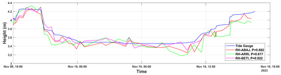
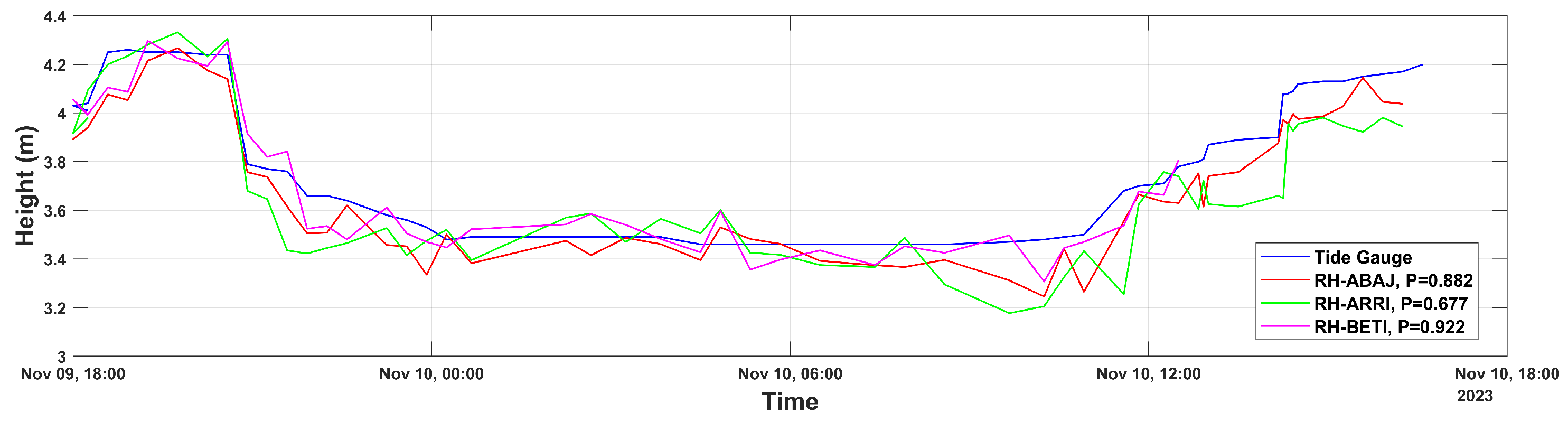
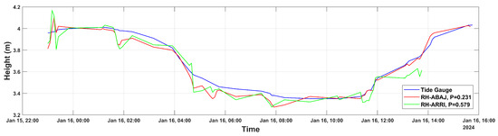
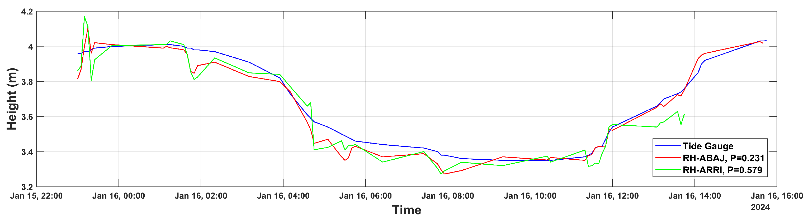
In addition, the time series of sea level data derived from both GNSS-R and tide gauge measurements for Campaign 1 (C-1) are shown in Figure 6. It can be observed that the GNSS-R measurements from the ARRI and ABAJ stations follow the same temporal trend as the relative sea-level measurements obtained from the conventional tide gauge. Likewise, some straight segments are visible in the GNSS-R time series, corresponding to short periods of missing data caused by interruptions in the power supply system.

Figure 6. Comparison of GNSS and tide gauge height trends over time, campaign one.

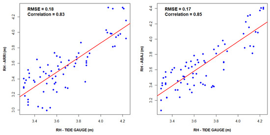
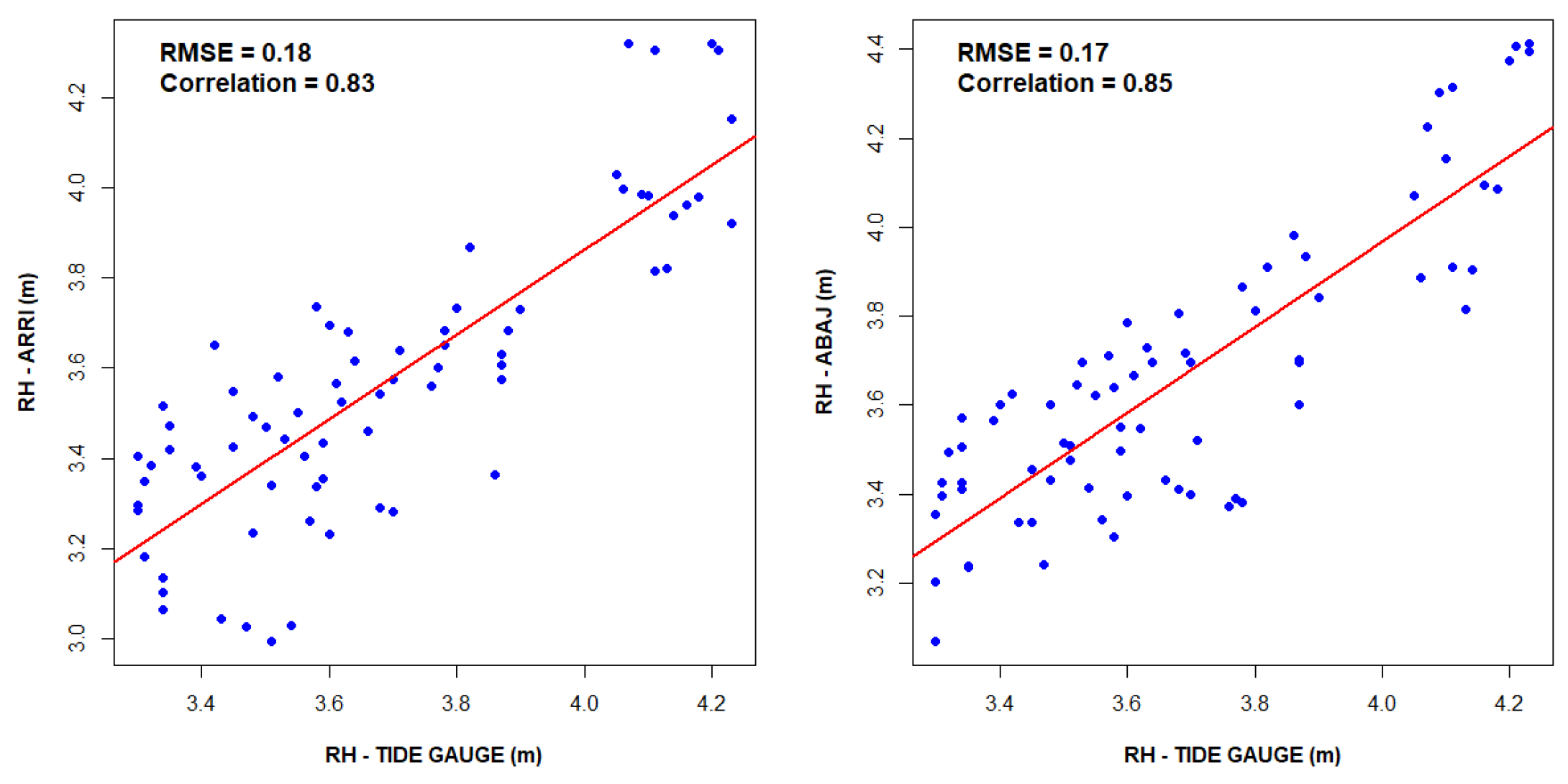
Furthermore, we performed a statistical comparison of the accuracy of sea-level measurements (GNSS-R) using linear correlation for each station with respect to the conventional tide gauge (Figure 7). It can be observed that, in both stations, the dispersion of the data is in the same direction as the diagonal, with a correlation of 0.83 (83%) for the ARRI station and a root mean square error (RMSE) of 0.18 m. Meanwhile, for the ABAJ station, the correlation between the measurements is equal to 0.85 with an RMSE of 0.17 m.

Figure 7. Linear correlation between sea-level measurements obtained from GNSS-R and the conventional tide gauge during Campaign 1. Blue dots represent individual observations and the red line corresponds to the linear regression fit. (Left panel) ARRI station; (right panel) ABAJ station.

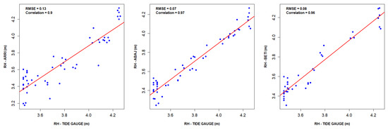
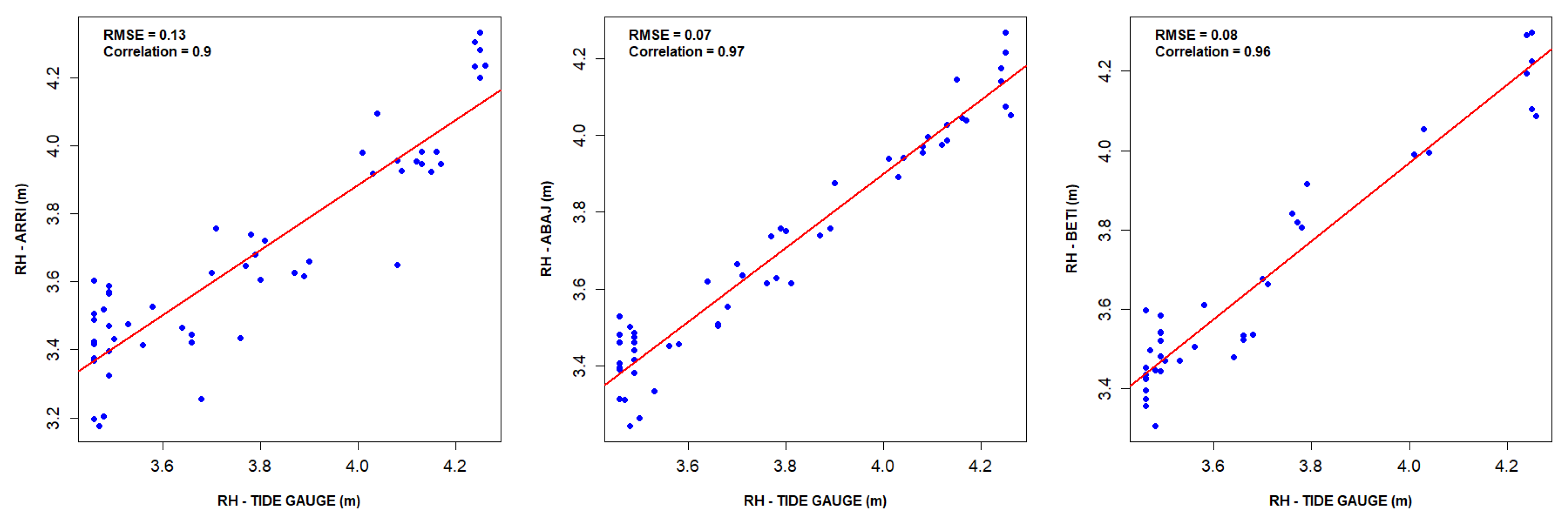
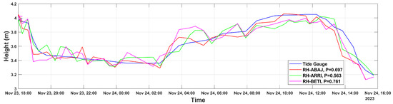
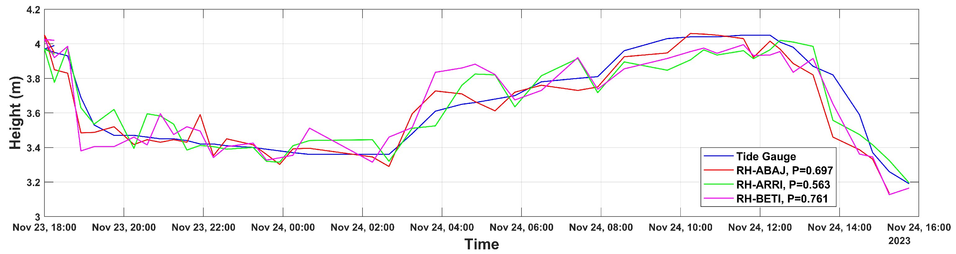
The measurement trends for campaigns C2–C5 are shown in Figure 8. It should be noted that, in these campaigns, the GNSS-R sea-level measurements exhibit a tidal behavior consistent with the heights recorded by the conventional tide gauge. Nevertheless, bias segments of approximately $3\mathrm{h}$ can be observed for the BETI station. These are attributable to signal loss between the receiver and the data storage system, likely caused by software handling errors. Strong linear correlations ($\rho$) were obtained for campaign C-2, with values of 0.97, 0.90, and 0.96 for stations ABAJ, ARRI, and BETI, respectively (Figure 9). Moreover, the root mean square errors (RMSEs) were computed, yielding values of $0.07\mathrm{m}$ for ABAJ, $0.13\mathrm{m}$ for ARRI, and $0.08\mathrm{m}$ for BETI.

Figure 8. Time series of relative sea-level measurements using GNSS-R and a conventional tide gauge for campaign C-2.

Figure 9. Linear correlation between sea-level measurements obtained from the GNSS-R tide gauge (GNSS-R TG) and the conventional tide gauge during Campaign C-2. Blue dots denote individual sea-level observations, and the red line represents the best-fit linear regression. The ARRI station is shown in the (left) panel, the ABAJ station in the (center) panel, and the BETI station in the (right) panel.

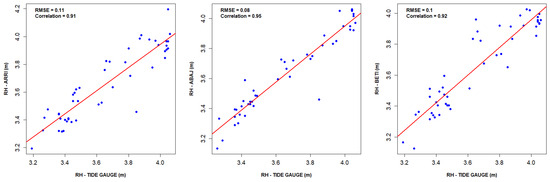
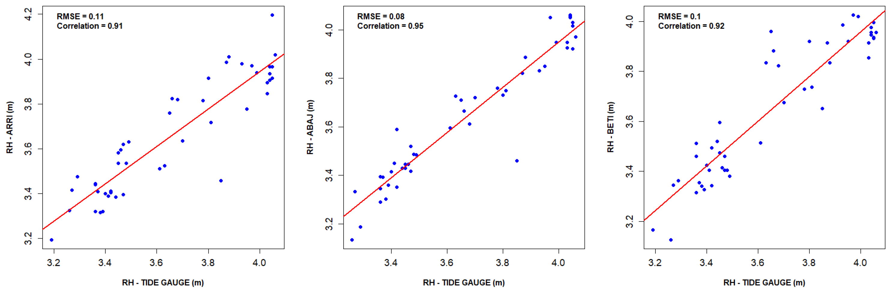
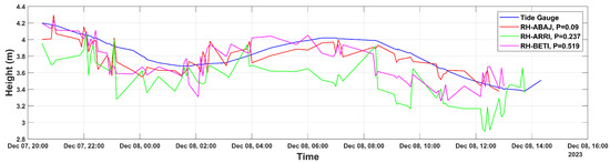
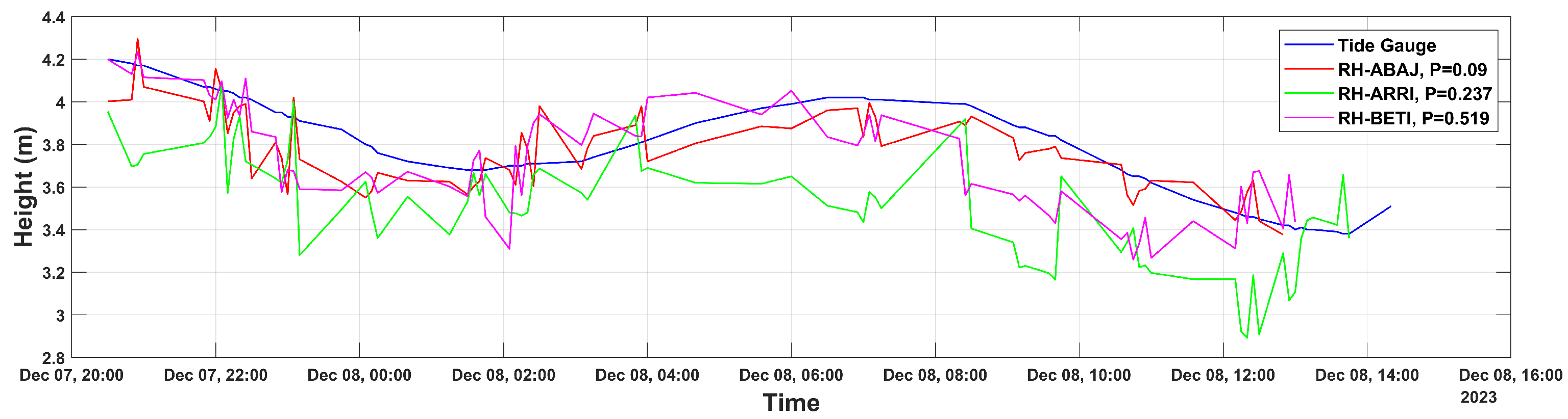
Figure 10 shows the trend of sea-level observations with respect to time, which is analogous to the tidal trend. In the latter, it can be observed that the variations between stations are relatively small, as demonstrated in the linear correlation statistics (Figure 11), with values of ($\rho$) 0.95, 0.91 and 0.92 for ABAJ, ARRI and BETI, respectively, and RMSEs of 0.08 m, 0.11 m, and 0.10 m, respectively.

Figure 10. Trend of relative sea-level measurements using GNSS-R and MC during campaign C-3.

Figure 11. Linear correlation between sea-level measurements obtained from the GNSS-R tide gauge (GNSS-R TG) and the conventional tide gauge during Campaign C-3. Blue dots represent paired sea-level observations, while the red line corresponds to the least-squares linear regression fit. The ARRI station is shown in the (left) panel, the ABAJ station in the (center) panel, and the BETI station in the (right) panel.

Sequentially, the C-4 campaign had the greatest measurement discrepancy, especially at the ARRI station, since it presented abrupt variations and biases between measurement intervals, caused by alterations in the antenna environment. Consequently, the remaining stations behaved in a similar way, presenting significant differences between measurements, since the antennas were installed in the same location. Nonetheless, the measurements followed the reference tidal trend, which can be seen in Figure 12. The preceding results are inferred to be heavily influenced by the immediate environment; visual observations noted fishing boats passing relatively close to the antennas, causing pronounced wake variations. However, because independent meteorological and wave-buoy data (e.g., significant wave height and wind speed) were not available during these campaigns, the direct correlation between GNSS-IR noise and quantitative sea-state conditions remains a limitation that should be addressed in future long-term deployments.

Figure 12. Trend of relative sea-level measurements using GNSS-R and MC during campaign C-4.

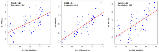
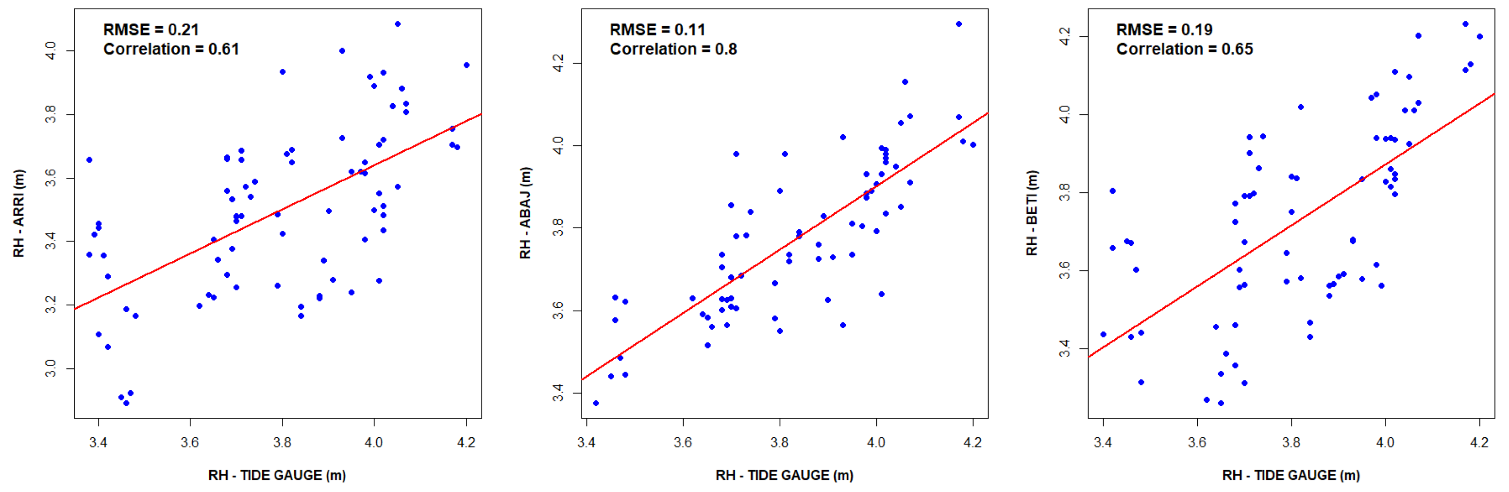
Additionally, the correlation metrics between measurements are represented in Figure 13. It can be noted that, with respect to the tide gauge, the ARRI station has a correlation index equal to 0.61 and an RMSE of 0.21 m, reflecting the behavior of the measurements described above, while the ABAJ and BETI stations present ($\rho$) values of 0.80 and 0.65 individually, with RMSE of 0.11 m and 0.19 m, respectively. The previous results can be attributed to the environment, since fishing boats pass relatively close to the antennas, which causes waves and pronounced variations and, in turn, noise in the measurements.

Figure 13. Linear correlation between sea-level measurements obtained from the GNSS-R tide gauge (GNSS-R TG) and the conventional tide gauge during Campaign C-4. Blue dots represent paired sea-level observations, while the red line corresponds to the least-squares linear regression fit. The ARRI station is shown in the (left) panel, the ABAJ station in the (center) panel, and the BETI station in the (right) panel.

In addition, the sea-level variations during campaign C-5 (Figure 14) followed the trend of the tide amplitudes. However, in both stations (ARRI and ABAJ), there are biases between the data; these can be identified in the sections where the amplitudes change abruptly.

Figure 14. Trend of relative sea-level measurements using GNSS-R and MC during campaign C-5.

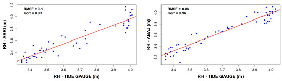
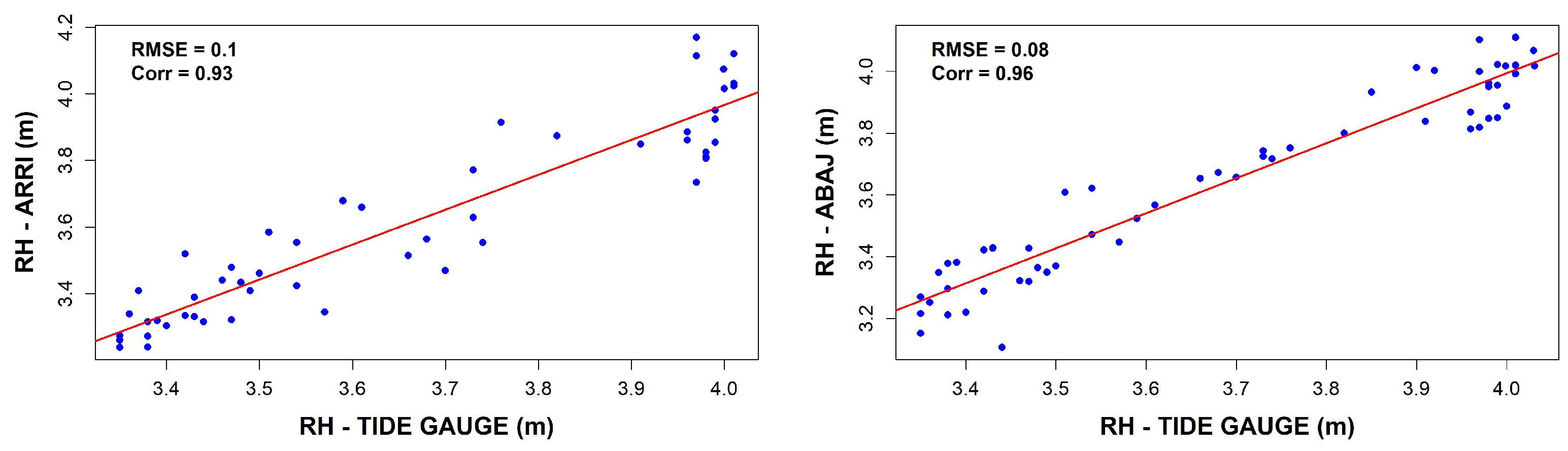
The observed correlation coefficients were 0.96 for the ABAJ station, with an RMSE of $0.08\mathrm{m}$, and 0.93 for the ARRI station, with an RMSE of $0.10\mathrm{m}$ (Table 4). It is worth noting that a data loss of approximately $6\mathrm{h}$ is evident, which is attributable to a power outage in the data storage system (Figure 15).

Figure 15. Linear correlation between sea-level measurements obtained from the GNSS-R tide gauge (GNSS-R TG) and the conventional tide gauge during Campaign C-5. Blue dots represent paired sea-level observations, while the red line corresponds to the least-squares linear regression fit. The ARRI station is shown in the (left) panel, and the ABAJ station is displayed in the (right) panel.

Statistical tests were conducted for each station and campaign to determine whether significant differences existed between the variances of the two measurement datasets, using a significance level of $\alpha =0.05$. Furthermore, the general statistics of the GNSS-R and tide gauge measurements per campaign are presented in Table 5.

Table 5. General statistics for measurement set by campaign.

Statistics per Station/Campaign
Station	Mean ($\overline{\mathit{y}}$)	Variance (${\mathit{S}}_{\mathit{i}}^{\mathbf{2}}$)	stDev ($\mathit{S}$)	Campaign
TIDE GAUGE	3.652873563	0.07302048	0.2717895	1
RH-ABAJ	3.663135135	0.1006715	0.3194535
RH-ARRI	3.565739726	0.10188033	0.3213959
TIDE GAUGE	3.791272727	0.08498565	0.2942099	2
RH-ABAJ	3.692814815	0.08156497	0.2882775
RH-ARRI	3.677277778	0.09316768	0.3080999
RH-BETI	3.6732	0.08158936	0.2892774
TIDE GAUGE	3.654042553	0.07670068	0.279943	3
RH-ABAJ	3.63673913	0.07010158	0.2676927
RH-ARRI	3.655957447	0.06460868	0.2569304
RH-BETI	3.649361702	0.07151427	0.2703127
TIDE GAUGE	3.787125	0.05225548	0.2300368	4
RH-ABAJ	3.77484507	0.03501233	0.1884476
RH-ARRI	3.494468354	0.06828574	0.2629852
RH-BETI	3.73390411	0.06052263	0.247716
TIDE GAUGE	3.710344828	0.06676195	0.26064	5
RH-ABAJ	3.641842105	0.08724452	0.2979974
RH-ARRI	3.615173077	0.07743872	0.2809931

Across all five measurement campaigns (C-1 to C-5), the statistical analysis demonstrates a consistent agreement between the GNSS-R measurements and the reference tide gauge data for the evaluated stations (ABAJ, ARRI, and BETI). In all cases, the computed F-statistics remained below their corresponding critical values and within the 95% confidence intervals (Table 6).

Table 6. Statistical test results for the five campaigns conducted.

Station	F (Tabulated)	F (Computed)	CI Lower	CI Upper	p-Value	Test Decision	Campaign
RH-ABAJ	1.5658	0.7253	0.4623	1.1242	0.149	$H_0$	1
RH-ARRI	1.5691	0.7167	0.4557	1.1121	0.1362	$H_0$
RH-ABAJ	1.7201	1.0416	0.605	1.789	0.882	$H_0$	2
RH-ARRI	1.7201	0.9118	0.53	1.566	0.736	$H_0$
RH-BETI	1.8297	1.0344	0.565	1.839	0.922	$H_0$
RH-ABAJ	1.803	1.094	0.605	1.968	0.764	$H_0$	3
RH-ARRI	1.803	1.094	0.605	1.968	0.764	$H_0$
RH-BETI	1.795	1.072	0.597	1.925	0.813	$H_0$
RH-ABAJ	1.586	1.490	0.939	2.349	0.09	$H_0$	4
RH-ARRI	1.562	0.765	0.489	1.194	0.237	$H_0$
RH-BETI	1.580	0.863	0.545	1.356	0.519	$H_0$
RH-ABAJ	1.694	0.764	0.451	1.294	0.316	$H_0$	5
RH-ARRI	1.722	0.860	0.499	1.470	0.579	$H_0$

CI: confidence interval; $H_0$: null hypothesis.

Furthermore, the associated p-values consistently exceeded the significance level of $\alpha =0.05$. Consequently, the null hypothesis ($H_0$) was accepted for all stations and campaigns, indicating that no statistically significant differences exist between the variances of the GNSS-R measurements and the tide gauge observations.

However, during campaign C-4, the ABAJ station yielded a relatively low p-value ($p=0.09$). Although this still satisfies the acceptance criterion for $H_0$, it suggests a borderline case that may reflect increased variability or potential systematic effects and therefore should be interpreted with caution.

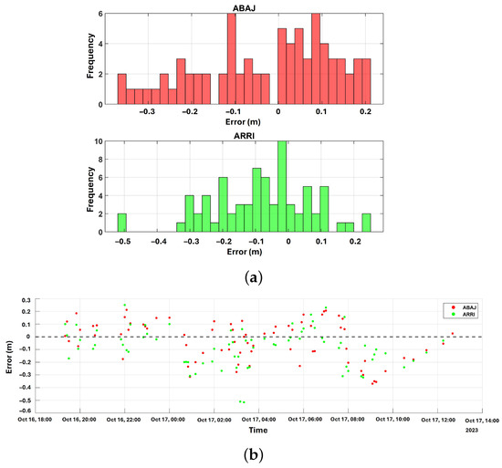
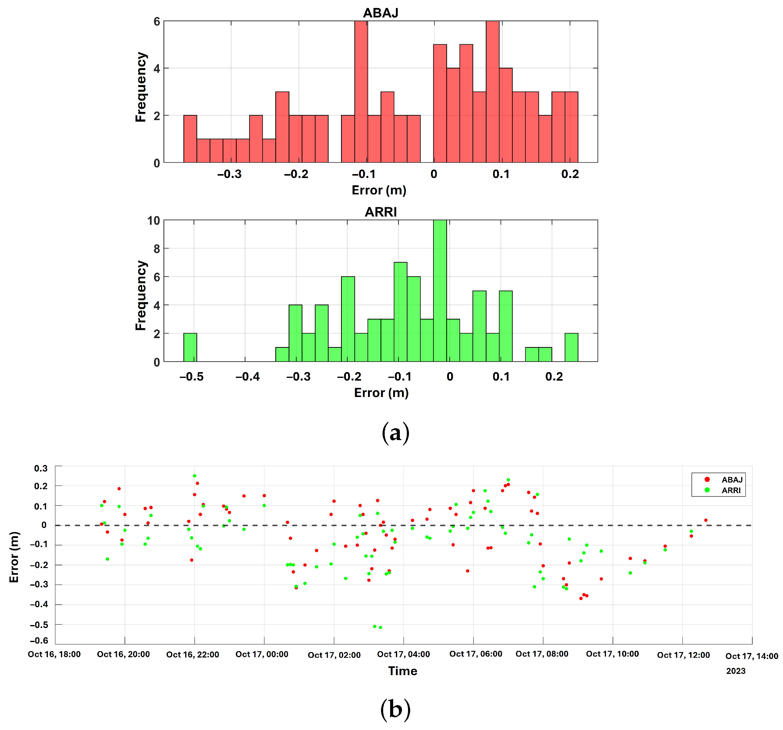
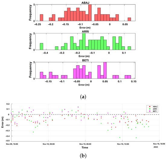
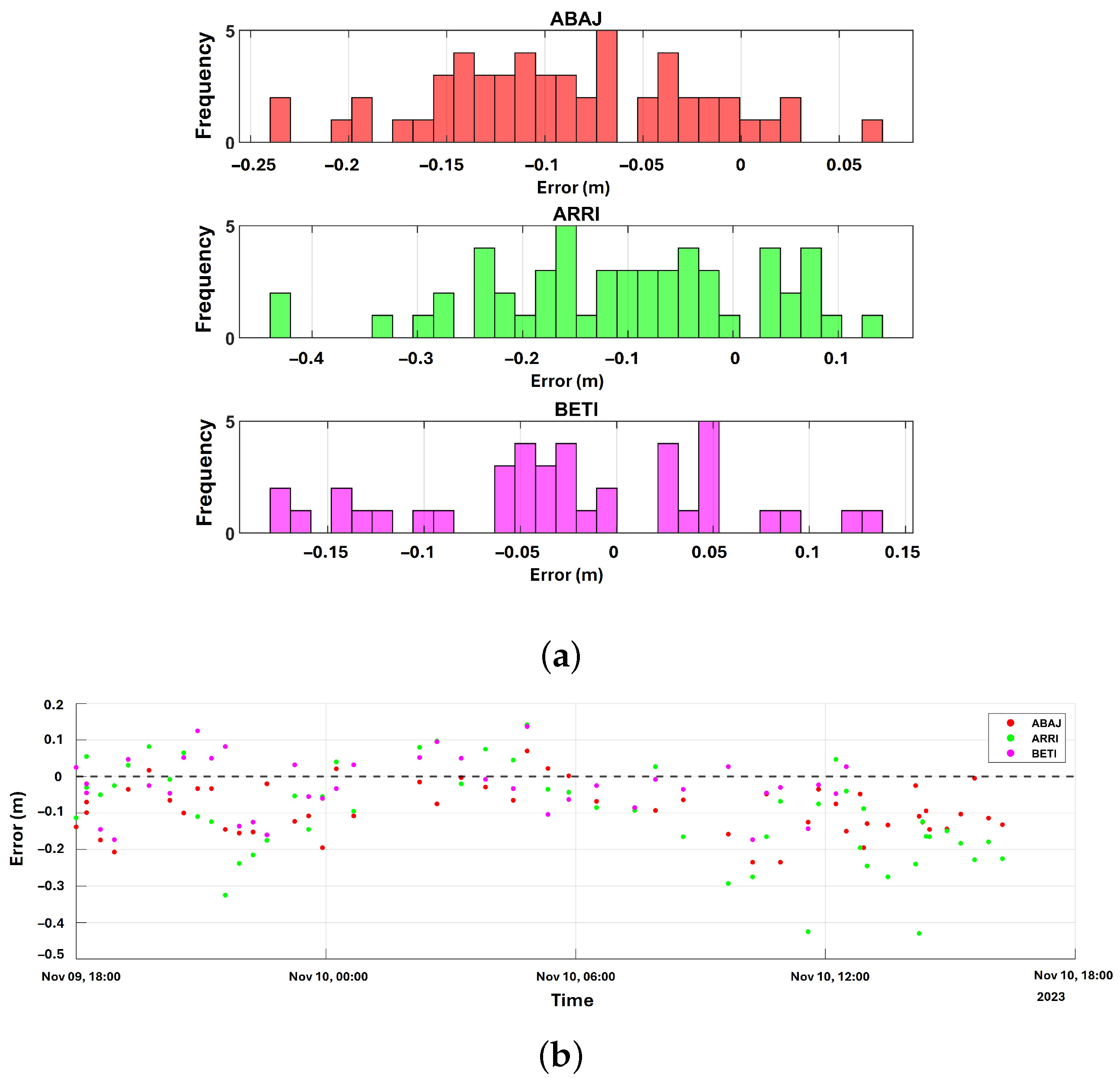
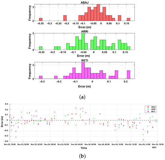
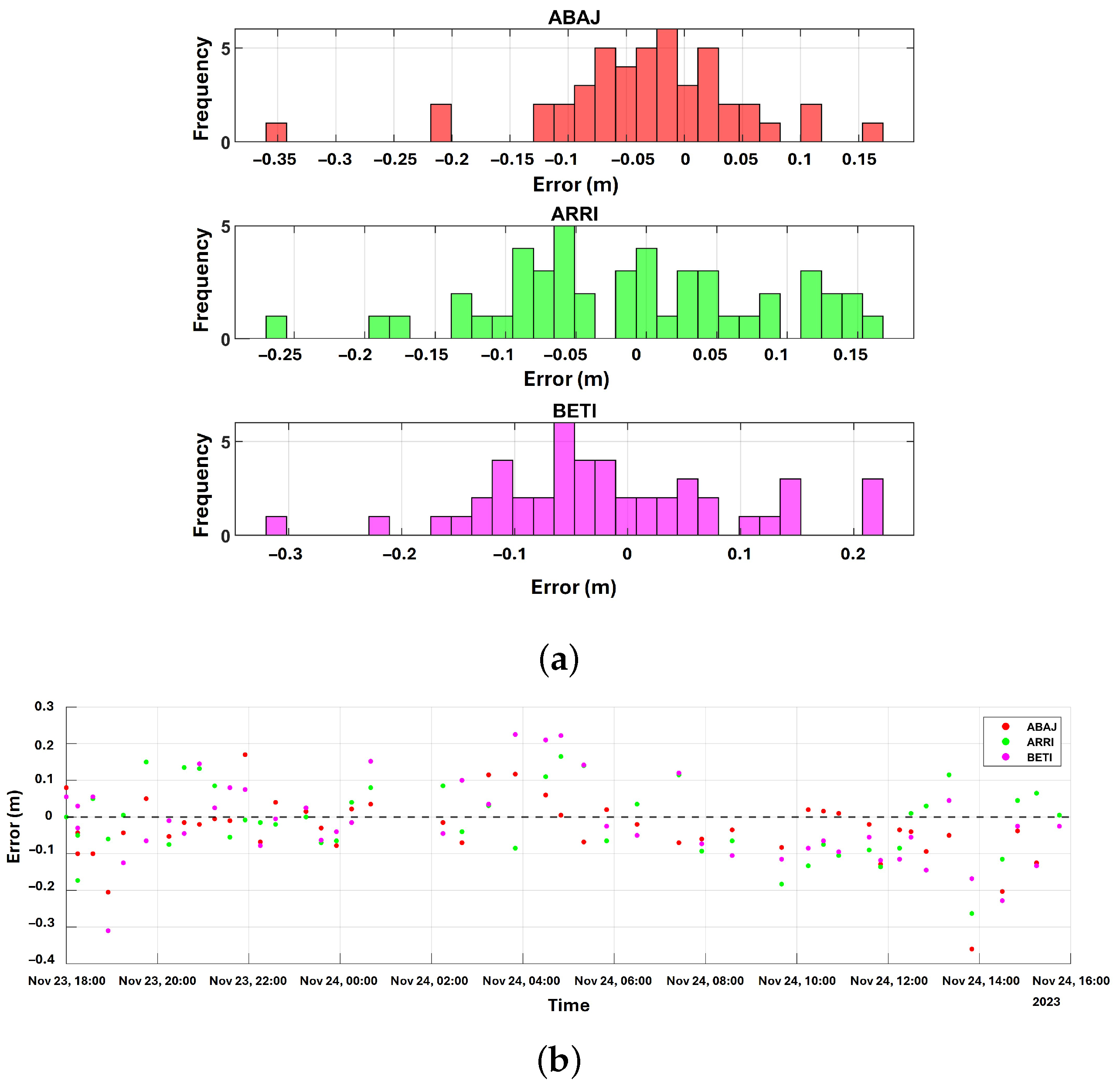
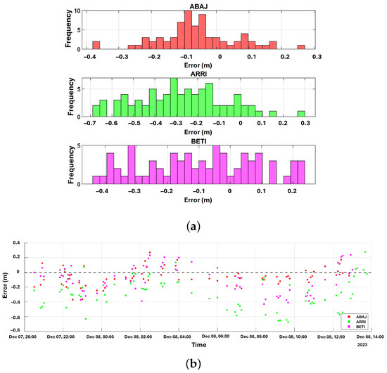
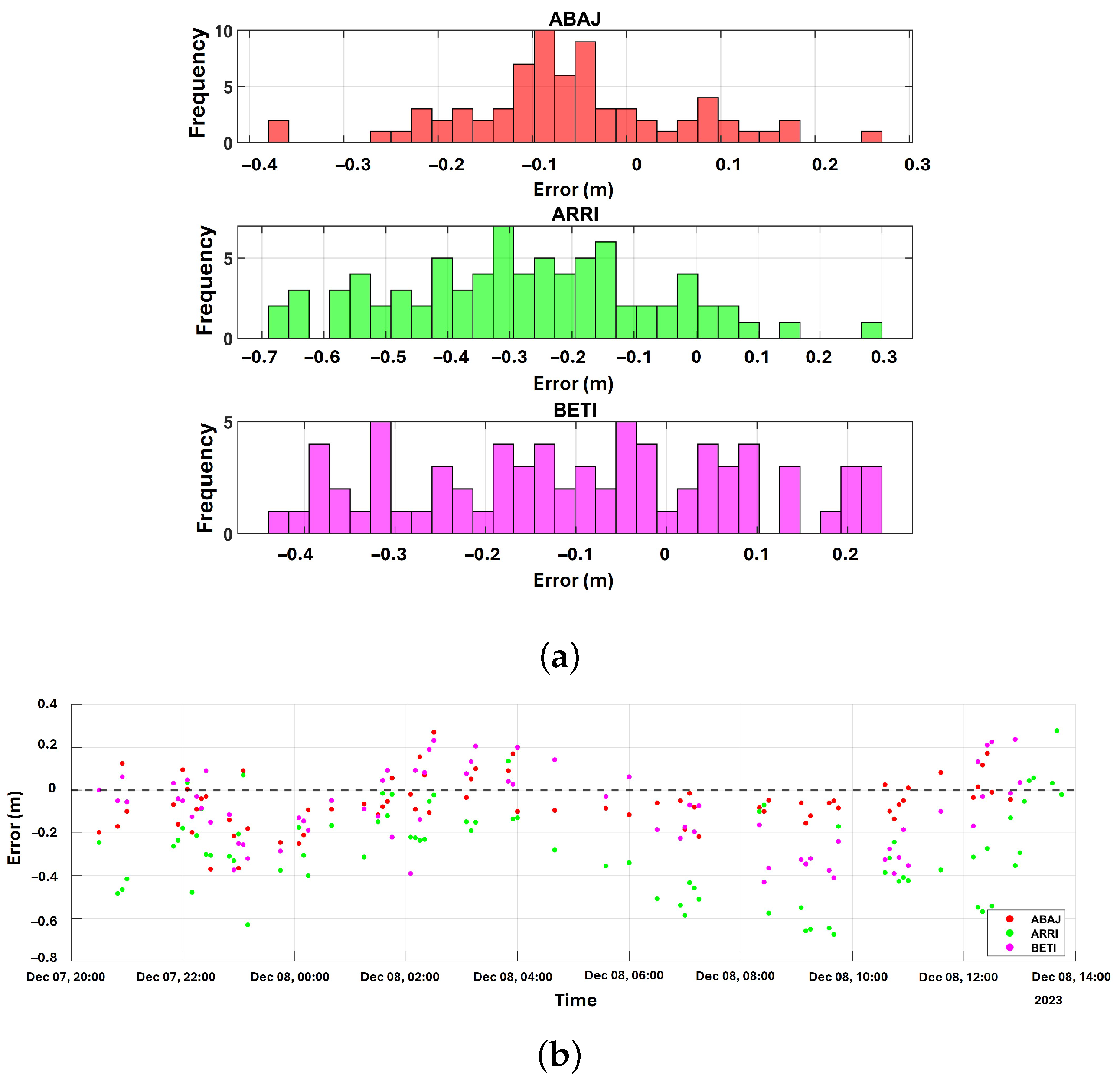
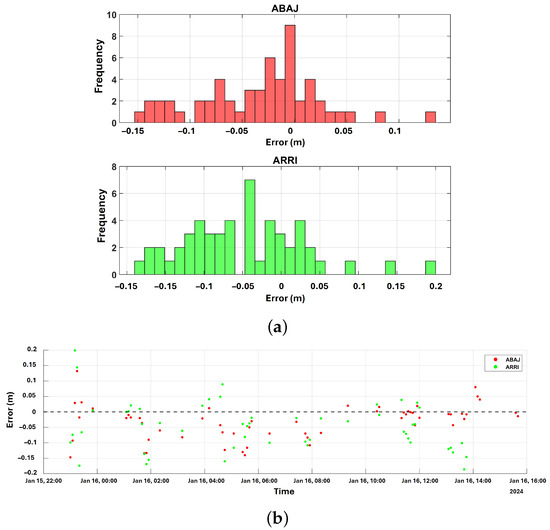
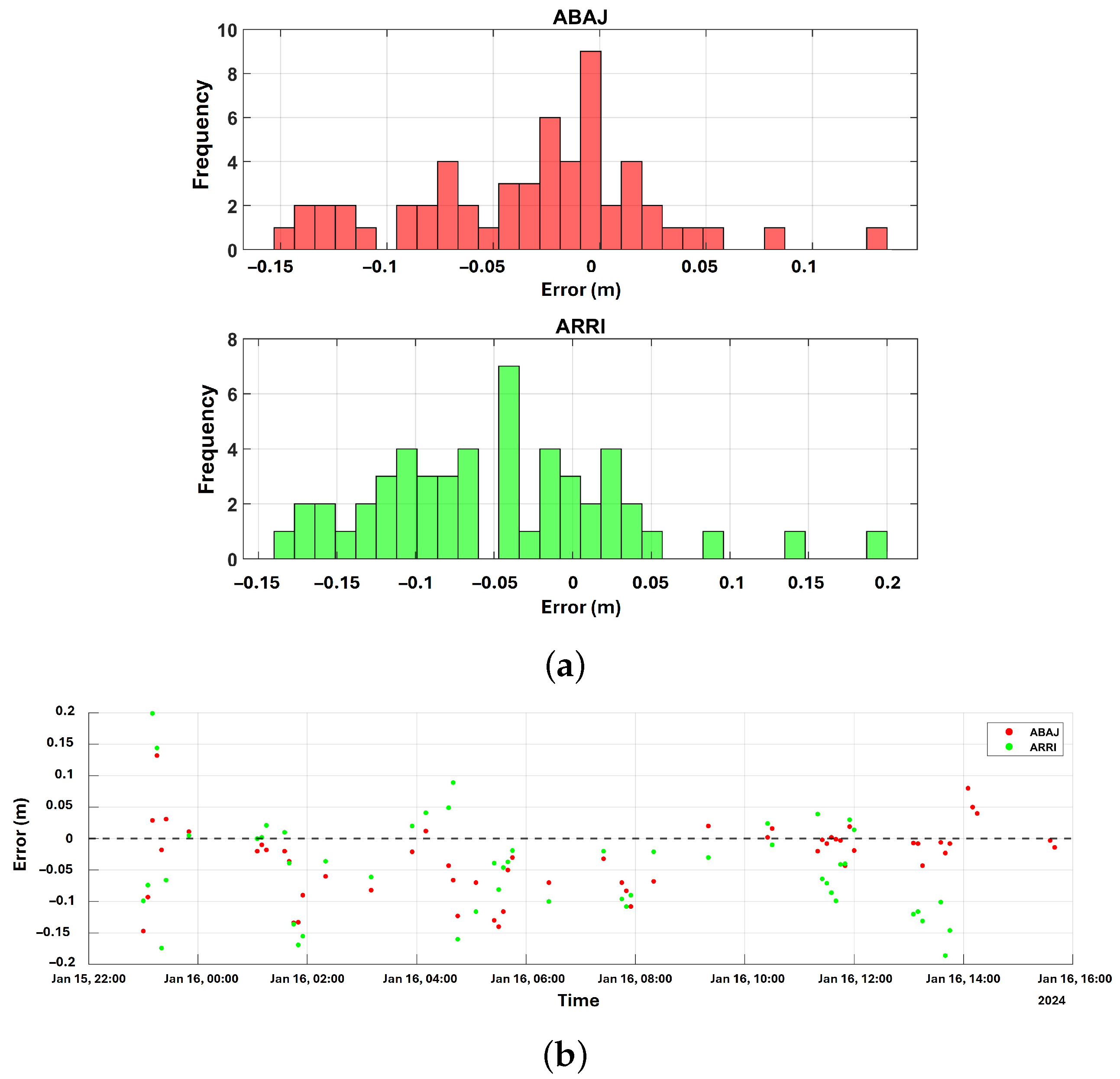
To further evaluate the robustness of the low-cost GNSS-IR system, a residual analysis was conducted. The residuals (defined as the differences between the GNSS-IR retrievals and the tide gauge reference data) were computed for all campaigns. The error distribution analysis (Figure 16, Figure 17, Figure 18, Figure 19 and Figure 20) indicates a near-normal distribution centered around zero, confirming the absence of severe systematic biases in the SNR inversions. The minor residual spread is primarily attributable to high-frequency wave action and environmental noise during specific tidal phases.

Figure 16. The error distribution analysis and frequency distribution (histogram) for the first campaign. (a) Frequency distribution (histogram). (b) Error distribution.

Figure 17. The error distribution analysis and frequency distribution (histogram) for the second campaign. (a) Frequency distribution (histogram). (b) Error distribution.

Figure 18. The error distribution analysis and frequency distribution (histogram) for the third campaign. (a) Frequency distribution (histogram). (b) Error distribution.

Figure 19. The error distribution analysis and frequency distribution (histogram) for the fourth campaign. (a) Frequency distribution (histogram). (b) Error distribution.

Figure 20. The error distribution analysis and frequency distribution (histogram) for the fifth campaign. (a) Frequency distribution (histogram). (b) Error distribution.

4. Discussion and Conclusions

From the analysis of coastal sea level data obtained using low-cost GNSS receivers, the feasibility of these devices under the GNSS reflectometry (GNSS-R) technique was evaluated. Signal-to-noise ratio (SNR) data were collected from three receiving antennas, each connected to an independent low-cost receiver. The analysis was conducted using only the GPS constellation.

Five measurement campaigns, each with a duration of approximately 24 h, were performed to assess the quality of the observations. An elevation mask of approximately 25° was applied to retrieve reflected SNR signals from the sea, whereas previous studies have reported elevation masks of up to 50° [37]. Additionally, the pre-processed SNR data within an azimuth range of 120° to 295° exhibited a damped sinusoidal behavior, consistent with the literature.

However, during low-tide conditions, exposed sand surfaces introduce significant noise into the measurements. As a result, the initial sea level retrievals exhibited relatively large root mean square (RMS) values, reaching up to $0.48\mathrm{m}$ for campaigns 1 and 2. After adjustments and height-rate corrections were applied, the RMS decreased substantially, reaching values of approximately $2\mathrm{cm}$ and $3.1\mathrm{cm}$, with the latter corresponding to campaign 1.

The final sea level estimates were compared against observations from a conventional tide gauge with a sampling interval of 1 min, later reduced to 5 min by the Mexican Navy (SEMAR). Consequently, the number of GNSS-R observations was also reduced, resulting in a loss of temporal resolution that may affect statistical variability (i.e., reduced precision).

The results show acceptable correlations ($\rho$), ranging from a minimum of 0.61 in campaign C-4 to a maximum of 0.97 in campaign C-2. The root mean square error (RMSE) ranges between $7.0\mathrm{cm}$ and $21.0\mathrm{cm}$. Previous studies using low-cost GNSS-IR systems have reported lower RMSE values under different environmental conditions and deployment configurations [5,37]. Similarly, Reference Fagundes et al. [5] analyzed one year of GNSS-R observations using a low-cost device, obtaining a correlation of 0.98 and an RMSE of $2.9\mathrm{cm}$ relative to a conventional tide gauge. Although the RMSE values obtained in this study (7–$21\mathrm{cm}$) are higher than those reported in previous low-cost GNSS-IR investigations, direct comparisons should be interpreted with caution because of differences in environmental conditions, tidal ranges, deployment durations, and experimental configurations. The present experiments were conducted in an environment with a low tidal range ($0.35$–$1.15\mathrm{m}$) using short-term field deployments affected by practical hardware limitations, including power interruptions and data storage failures. Consequently, the main contribution of this work is not the achievement of the lowest RMSE but rather the demonstration that a low-cost GNSS-IR architecture based on commercially available receivers can successfully reproduce sea-level variability and maintain statistical consistency with an operational tide gauge under real-world coastal conditions.

It was hypothesized, on the basis of visual observations during the campaign, that this degradation was caused by the wakes of nearby fishing boats altering the surface roughness. However, for lack of independent auxiliary data (such as wave buoy measurements or port traffic logs), this remains an unverified inference. While increasing the minimum elevation cut-off angle to $10°$ could theoretically shrink the Fresnel zone and filter out distant wave interference, applying this restriction to a GPS-only dataset critically limits the number of valid satellite arcs, severely degrading the temporal continuity of the sea-level retrievals.

The combination of low-cost antennas and receivers proved capable of capturing sea-level variations using GNSS-R. In fact, [37] demonstrated that low-cost antennas can outperform geodetic antennas in certain configurations, particularly when operating at elevation masks greater than $30°$. Furthermore, these systems represent a practical alternative due to their lower cost, portability, and ease of deployment.

To validate the obtained results and assess the presence of systematic errors, a statistical analysis was conducted. The null hypothesis ($H_0$) assumes equality between the variances of GNSS-R and tide gauge measurements. Fisher’s F-test was applied, as the data satisfied the required conditions, including independence and approximate normality.

The results confirm the reliability of the GNSS-R observations, as the null hypothesis was accepted for all campaigns at a 95% confidence level. This indicates that the computed F-statistic falls within the acceptance region, i.e., below the critical F-value. It should be noted that the F-test evaluates the equality of variances between the GNSS-R and tide gauge measurements rather than the equality of the time series themselves. Therefore, the acceptance of $H_0$ indicates that the two datasets exhibit statistically comparable variability and dynamic range, whereas the temporal agreement and phase-tracking capability are assessed through the correlation analysis and residual evaluation presented in the previous sections.

It is important to acknowledge the limitations of the current experimental design. The five measurement campaigns, lasting approximately $24\mathrm{h}$ each, successfully demonstrate short-term technical feasibility and statistical agreement with the reference tide gauge. However, these short durations are insufficient to evaluate the long-term durability of low-cost hardware (e.g., susceptibility to salt corrosion or prolonged power interruptions) compared to established tide gauge infrastructure. Furthermore, a continuous deployment of at least one full lunar cycle (∼29 days) is required in future studies to rigorously assess the system’s performance across the complete spectrum of spring and neap tidal phases. Likewise, extended deployments would enable the assessment of long-term hardware stability; measurement drift; and the influence of environmental factors such as wind waves, temperature fluctuations, and salinity variations.

While the low-cost GNSS receivers demonstrated high accuracy in sea-level retrieval, the data gaps encountered in campaigns 3 and 5 highlight a significant practical vulnerability in the power and data-logging infrastructure. For long-term, autonomous coastal deployments, makeshift storage (e.g., standard laptops) and reliance on local pier power grids are insufficient. Future implementations must incorporate redundancy strategies, such as the use of dedicated low-power microcontrollers (e.g., Raspberry Pi or Arduino-based loggers), integrated solar-panel and battery-bank subsystems, and IoT (Internet of Things) telemetry for real-time remote monitoring and data transmission. Although the u-blox ZED-F9P is a multi-constellation receiver, this initial study restricted processing to GPS-only signals to establish a baseline validation using the most mature algorithms within the open-source gnssrefl environment. We fully acknowledge that this limitation underutilizes the hardware’s potential. Incorporating multi-constellation data (GLONASS, Galileo, BeiDou) in future processing will drastically increase the number of valid daily satellite arcs, thereby enhancing both the temporal resolution and the spatial coverage of the coastal reflection zones.

The benchmarking results presented in Table 7 suggest that several factors may explain the large RMSE values obtained in the present study compared with previous low-cost GNSS-IR investigations. First, the measurement campaigns were limited to short-term deployments (17–23 h), whereas other studies relied on observations spanning several months or even one year. Second, only GPS observations were processed, reducing the number of available satellite arcs compared with multi-constellation approaches. Third, occasional power interruptions and data storage failures introduced data gaps that affected the continuity of the observations. Finally, the relatively small tidal range observed at Altata Bay (0.35–1.15 m) reduces the dynamic range of the signal, making the retrievals more sensitive to measurement noise and environmental disturbances. Consequently, although the RMSE values reported here are larger than those obtained in previous studies, the proposed system successfully demonstrated the feasibility of low-cost GNSS-IR monitoring under realistic coastal operating conditions.

Table 7. Benchmarking of recent low-cost GNSS-IR sea-level monitoring studies compared to the present work.

Reference	Hardware/Receiver	Method	Tidal Range	Temporal Coverage	RMSE vs. Tide Gauge
Fagundes et al. [5]	Low-cost open-source	SNR	∼1.5 m	1 year	$2.9\mathrm{cm}$
Knight et al. [26]	Low-cost GNSS buoy	GNSS RTK	∼4.0 m	Short-term	$1.4\mathrm{cm}$
Bell et al. [28]	Low-cost GNSS	SNR	>$3.0\mathrm{m}$	Months	$1.7\mathrm{cm}$
This study	u-blox ZED-F9P	SNR inversion	∼1.15 m	5 campaigns (∼24 h)	$7.0$–$21.0\mathrm{cm}$

RMSE: root mean square error; RTK: real-time kinematic; SNR: signal-to-noise ratio.

The principal contribution of this study is not the achievement of the lowest RMSE values reported in the literature but rather the demonstration that a low-cost GNSS-IR architecture based on commercially available receivers can reliably reproduce sea-level variability under real-world coastal monitoring conditions. Furthermore, the analysis of height-rate and inter-frequency corrections, together with the statistical validation against an operational tide gauge, provides additional insight into the performance and limitations of low-cost GNSS-IR systems deployed in low-tidal-range environments.

Ultimately, it can be concluded that low-cost GNSS receivers are capable of retrieving sea-level measurements with RMSE values ranging from $7.0$ to $21.0\mathrm{cm}$ during short-term (∼24 h) campaigns while successfully reproducing the temporal variability observed in the reference tide gauge records. Although these errors are larger than those reported in some previous low-cost GNSS-IR studies (Table 7), direct comparisons should be interpreted with caution because of differences in tidal range, deployment duration, environmental conditions, and experimental configurations. The proposed low-cost GNSS-IR system nevertheless demonstrated statistically consistent performance with the reference tide gauge under real coastal monitoring conditions. Therefore, low-cost GNSS antennas and receivers constitute a viable and cost-effective alternative for expanding coastal sea-level monitoring networks using GNSS-R.

References

- Lyros, E.; Kostelecky, J.; Plicka, V.; Vratislav, F.; Sokos, E.; Nikolakopoulos, K. Detection of Tectonic and Crustal Deformation Using GNSS Data Processing: The Case of PPGnet. Civ. Eng. J. 2021, 7, 14–23. [Google Scholar] [CrossRef] [Scilit]
- Nayak, K.; Romero-Andrade, R.; Sharma, G.; Colonna, R. Sequential Evolution of Ionospheric TEC Anomalies and Acoustic-Gravity Wave Precursors Associated with the February 8, 2025, Mw 7.6 Cayman Islands Earthquake. J. Atmos. Sol.-Terr. Phys. 2025, 274, 106582. [Google Scholar] [CrossRef] [Scilit]
- Bezcioglu, M.; Yigit, C.O.; Mazzoni, A.; Fortunato, M.; Dindar, A.A.; Karadeniz, B. High-Rate (20 Hz) Single-Frequency GPS/GALILEO Variometric Approach for Real-Time Structural Health Monitoring and Rapid Risk Assessment. Adv. Space Res. 2022, 70, 1388–1405. [Google Scholar] [CrossRef] [Scilit]
- Larson, K.M.; Ray, R.D.; Williams, S.D.P. A 10-Year Comparison of Water Levels Measured with a Geodetic GPS Receiver versus a Conventional Tide Gauge. J. Atmos. Ocean. Technol. 2017, 34, 295–307. [Google Scholar] [CrossRef] [Scilit]
- Fagundes, M.A.R.; Mendonça-Tinti, I.; Iescheck, A.L.; Akos, D.M.; Geremia-Nievinski, F. An Open-Source Low-Cost Sensor for SNR-Based GNSS Reflectometry: Design and Long-Term Validation towards Sea-Level Altimetry. GPS Solut. 2021, 25, 73. [Google Scholar] [CrossRef] [Scilit]
- IPCC. Climate Change 2021: The Physical Science Basis. Contribution of Working Group I to the Sixth Assessment Report of the Intergovernmental Panel on Climate Change; Cambridge University Press: Cambridge, UK, 2021. [Google Scholar] [CrossRef] [Scilit]
- Alonso-Arroyo, A.; Camps, A.; Park, H.; Pascual, D.; Onrubia, R.; Martin, F. Retrieval of Significant Wave Height and Mean Sea Surface Level Using the GNSS-R Interference Pattern Technique. IEEE Trans. Geosci. Remote Sens. 2015, 53, 3198–3209. [Google Scholar] [CrossRef] [Scilit]
- Cazenave, A.; Nerem, R.S. Present-Day Sea Level Change: Observations and Causes. Rev. Geophys. 2004, 42, 2003RG000139. [Google Scholar] [CrossRef] [Scilit]
- Watson, C.; Coleman, R.; Handsworth, R. Coastal Tide Gauge Calibration. J. Coast. Res. 2008, 244, 1071–1079. [Google Scholar] [CrossRef] [Scilit]
- Salama, G.M.; Hamed, H.F.A.; Deabes, E.A.M.; Othman, S.E. Innovative Mechanical Tide Gauge Improvement. Meas. Sens. 2019, 100005. [Google Scholar] [CrossRef] [Scilit]
- Martín Míguez, B.; Testut, L.; Wöppelmann, G. Modern Tide Gauges Performance. Sci. Mar. 2012, 76, 221–228. [Google Scholar] [CrossRef] [Scilit]
- Nerem, R.S.; Leuliette, É.; Cazenave, A. Sea-Level Change Review. C. R. Geosci. 2006, 338, 1077–1083. [Google Scholar] [CrossRef] [Scilit]
- Cazenave, A.; Moreira, L. Sea-Level Changes Review. Proc. R. Soc. A 2022, 478, 20220049. [Google Scholar] [CrossRef] [Scilit] [PubMed]
- Peng, D.; Feng, L.; Larson, K.M.; Hill, E.M. GNSS-IR Sea-Level Measurement. Remote Sens. 2021, 13, 4319. [Google Scholar] [CrossRef] [Scilit]
- Lowe, S.T.; LaBrecque, J.L.; Zuffada, C.; Romans, L.J.; Young, L.E.; Hajj, G.A. Earth-Reflected GPS Signal. Radio Sci. 2002, 37. [Google Scholar] [CrossRef] [Scilit]
- Martin-Neira, M. A Passive Reflectometry and Interferometry System (PARIS) Application to Ocean Altimetry. ESA J. 1993, 17, 142–150. [Google Scholar]
- Soulat, F.; Caparrini, M.; Germain, O.; Lopez-Dekker, P.; Taani, M.; Ruffini, G. GNSS-R Sea State Monitoring. Geophys. Res. Lett. 2004, 31, L21303. [Google Scholar] [CrossRef] [Scilit]
- Löfgren, J.S.; Haas, R.; Scherneck, H.G.; Bos, M.S. Local Sea Level from GNSS. Radio Sci. 2011, 46, 1–12. [Google Scholar] [CrossRef] [Scilit]
- Anderson, K.D. Water Level from GPS. J. Atmos. Ocean. Technol. 2000, 17, 1118–1127. [Google Scholar] [CrossRef] [Scilit]
- Larson, K.M.; Ray, R.D.; Nievinski, F.G.; Freymueller, J.T. Accidental Tide Gauge. IEEE Geosci. Remote Sens. Lett. 2013, 10, 1200–1204. [Google Scholar] [CrossRef] [Scilit]
- Nievinski, F.G.; Larson, K.M. GPS Multipath Modeling I. IEEE Trans. Geosci. Remote Sens. 2014, 52, 6555–6563. [Google Scholar] [CrossRef] [Scilit]
- Nievinski, F.G.; Larson, K.M. GPS Multipath Modeling II. IEEE Trans. Geosci. Remote Sens. 2014, 52, 6564–6573. [Google Scholar] [CrossRef] [Scilit]
- Strandberg, J.; Hobiger, T.; Haas, R. GNSS-R Sea Level Improvement. Radio Sci. 2016, 51, 1286–1296. [Google Scholar] [CrossRef] [Scilit]
- Martinez-Felix, C.A.; Vazquez-Becerra, G.E.; Geremia-Nievinski, F.; Millan-Almaraz, J.R.; Franco-Ochoa, C.; Melgarejo-Morales, A.; Gaxiola-Camacho, J.R. Tidal Measurements Comparison. GPS Solut. 2022, 26, 22. [Google Scholar] [CrossRef] [Scilit]
- Ichikawa, K.; Ebinuma, T.; Konda, M.; Yufu, K. Low-Cost GNSS-R UAV. Sensors 2019, 19, 998. [Google Scholar] [CrossRef] [Scilit] [PubMed]
- Knight, P.J.; Bird, C.O.; Sinclair, A.; Plater, A.J. A Low-Cost GNSS Buoy Platform for Measuring Coastal Sea Levels. Ocean Eng. 2020, 203, 107198. [Google Scholar] [CrossRef] [Scilit]
- Miguez, B.M.; Testut, L.; Wöppelmann, G. Van de Casteele Test. J. Atmos. Ocean. Technol. 2008, 25, 1238–1244. [Google Scholar] [CrossRef] [Scilit]
- Williams, S.D.P.; Bell, P.S.; McCann, D.L.; Cooke, R.; Sams, C. Low-Cost GPS for Tides. J. Atmos. Ocean. Technol. 2020, 37, 1925–1935. [Google Scholar] [CrossRef] [Scilit]
- Di, M.; Guo, B.; Ren, J.; Li, M.; Chen, X.; Zhang, A. GNSS Buoy Sea Surface Height. Ocean Eng. 2023, 277, 114362. [Google Scholar] [CrossRef] [Scilit]
- Larson, K.M. GNSS-IR Applications Review. WIREs Water 2016, 3, 775–787. [Google Scholar] [CrossRef] [Scilit]
- Hazel, P.; Herczeg, Z. u-Center; u-blox AG: Thalwil, Switzerland, 2021. [Google Scholar]
- Takasu, T.; Kubo, N.; Yasuda, A. Development, Evaluation and Application of RTKLIB: A Program Library for RTK-GPS. In Proceedings of the GNSS 2007, Tokyo, Japan, 20–22 November 2007. [Google Scholar]
- Larson, K.M. gnssrefl Software. GPS Solut. 2024, 28, 165. [Google Scholar] [CrossRef] [Scilit]
- Chen, L.; Chai, H.; Zheng, N.; Wang, M.; Xiang, M. Low-Cost GNSS-IR Performance. Adv. Space Res. 2023, 72, 4651–4662. [Google Scholar] [CrossRef] [Scilit]
- Löfgren, J.S.; Haas, R. Multi-Frequency Sea Level. EURASIP J. Adv. Signal Process. 2014, 2014, 50. [Google Scholar] [CrossRef] [Scilit]
- Ghilani, C.D. Adjustment Computations: Spatial Data Analysis, 5th ed.; Wiley: Hoboken, NJ, USA, 2010. [Google Scholar]
- Purnell, D.J.; Gomez, N.; Minarik, W.; Porter, D.; Langston, G. Precise Water Level Measurements. Earth Surf. Dyn. 2021, 9, 673–685. [Google Scholar] [CrossRef] [Scilit]
Disclaimer/Publisher’s Note: The statements, opinions and data contained in all publications are solely those of the individual author(s) and contributor(s) and not of MDPI and/or the editor(s). MDPI and/or the editor(s) disclaim responsibility for any injury to people or property resulting from any ideas, methods, instructions or products referred to in the content. |
© 2026 by the authors. Licensee MDPI, Basel, Switzerland. This article is an open access article distributed under the terms and conditions of the Creative Commons Attribution (CC BY) license.