


Highlights
What are the main findings?
- A kinematic orbit determination approach based on onboard GNSS code pseudorange measurements achieved a 3D RMSE of 49.6 cm for Sentinel-6A, without dynamic models or carrier-phase integer ambiguity resolution.
- Compared with the SPP, the final solution reduced the 3D RMSE from 101.2 cm to 49.6 cm and the radial bias from 52.7 cm to 1.4 cm.
What are the implications of the main findings?
- The results demonstrate that sub-meter real-time LEO kinematic orbit determination is feasible based on code pseudorange measurements.
- The proposed method offers a lightweight orbit determination strategy for future LEO PNT services and resource-constrained small-satellite constellations.
Abstract
The emerging potential of low-Earth-orbit (LEO) satellite-based Positioning, Navigation, and Timing services has increased the need for real-time, stable, and accurate orbit determination techniques. Here, we propose a method for estimating sub-meter-level LEO satellite orbits using Global Navigation Satellite System (GNSS) code pseudorange observations. To mitigate ionospheric delay, a dual-frequency ionosphere-free combination was applied, while code-carrier smoothing was employed to reduce code observation noise. A satellite weighting model based on Signal-in-Space Range Error was developed to reflect the orbit and clock error characteristics of different GNSS, and a robust weighting scheme was applied to alleviate the impact of observation outliers. Further, Galileo High Accuracy Service corrections compensated for orbit, clock and code bias errors. The algorithm was validated using the GNSS observation data collected from the Sentinel-6A satellite on 10 August 2023. Each successively applied technique gradually improved orbit determination accuracy, achieving up to a 51% reduction in 3D root mean square error (RMSE). The final RMSE values in the radial, along-track, cross-track, and 3D components were 39.4, 18.8, 23.5, and 49.6 cm, respectively. Temporal analysis showed no distinct periodicity in orbit errors and no significant correlation with satellite visibility or ground track.
1. Introduction
Recently, positioning technologies utilizing low-Earth-orbit (LEO) satellites have garnered significant attention as promising alternatives to overcome the limitations of existing Global Navigation Satellite System (GNSS) [1,2,3,4]. In particular, LEO satellites exhibit high signal strength and large Doppler shifts owing to their low altitude, and the concepts of Positioning, Navigation, and Timing (PNT) augmentation utilizing these features are being actively researched. These characteristics enable rapid geometric changes and a high Signal-to-Noise Ratio (SNR) compared to GNSS, thereby increasing the potential for utilizing LEO satellites as next-generation satellite navigation systems. However, accurate orbital information from LEO satellites is essential for real-time LEO PNT services [5]. Therefore, precise orbit determination of LEO satellites is a prerequisite for accurate positioning of LEO PNT service users.
Generally, satellite orbit determination is conducted using the Dynamic Orbit Determination (DOD) method, which relies on accurate modeling of external forces acting on the satellite and numerical integration for state propagation [6]. However, unlike Medium-Earth-Orbit (MEO) satellites, LEO satellites are significantly affected by atmospheric drag and higher-order perturbations of the Earth’s gravitational field; consequently, they require sophisticated force models and empirical parameter estimation, making them susceptible to modeling errors and leading to complex algorithm structures [7]. In particular, for real-time applications, precise force modeling and parameter estimation increase the computational burden, limiting system implementation [8]. GNSS observations significantly improve DOD accuracy [9]. With advances in GNSS receiver performance, GNSS-based orbit determination techniques have been applied to various LEO satellites and are widely used for missions that require precise orbit determination [10]. Real-time GNSS-based orbit determination methods using onboard LEO receiver observations are categorized into Reduced-Dynamic Orbit Determination (RDOD) and Kinematic Orbit Determination (KOD).
RDOD estimates the orbit of an LEO satellite by predicting its state using a dynamic model and updating it with GNSS observations. This enables robust orbit determination, even under unfavorable observation geometries or in the presence of outliers. Furthermore, the orbit can be propagated over short-term observation gaps using a dynamic model, thereby maintaining a continuous and accurate orbit estimate. In [11], they introduced the RDOD technique and demonstrated, through covariance analysis, that it outperformed both the dynamic and GPS measurement-based approaches in orbit accuracy. Subsequently, batch least-squares and extended Kalman filter approaches for RDOD were compared in [12], demonstrating that both methods could achieve centimeter-level accuracy. In [13,14], they reported the feasibility of GNSS-based real-time onboard orbit determination of LEO satellites using broadcast ephemerides, achieving decimeter-level accuracy and demonstrating performance improvements with multi-constellation processing. In addition, pseudo-ambiguity parameters were introduced in [15] to reduce line-of-sight (LOS) errors caused by the GPS broadcast ephemeris, achieving a 3D RMSE of approximately 40 cm. In [16], they applied the Piecewise Constant Acceleration (PCA) model to RDOD and achieved a 3D root mean square error (RMSE) of approximately 4.5 cm using CHAMP and GRACE satellite data for validation. Furthermore, ref. [17] proposed a Kalman filter-based RDOD technique that simplifies the dynamic model, demonstrating its ability to achieve meter-level accuracy in real time. More recently, ref. [18] applied the Ambiguity Resolution (AR) technique to RDOD and reported a 3D RMSE of approximately 6.5 cm. However, similar to DOD, RDOD requires accurate dynamic modeling and proper tuning of the empirical parameters, making its orbit determination performance susceptible to modeling errors [19,20,21].
In contrast, KOD estimates the satellite state based solely on GNSS observations without the use of a dynamical model. Consequently, this approach is unaffected by errors in the dynamic model and has a relatively simple computational structure. In [22], they proposed a zero-difference KOD technique and achieved a positioning accuracy of approximately 5 cm using GRACE satellite data. Furthermore, ref. [23] demonstrated that a piecewise linear receiver clock model improved KOD accuracy by at least 40% in the radial direction and up to 7% in the along-track and cross-track directions. In addition, ref. [24] presented an iterative least-squares-based KOD method using only GNSS raw observations and reported sub-centimeter accuracy. In [25], they proposed a real-time KOD technique using a single-frequency receiver, mitigating ionospheric delay errors using the GRoup And Phase Ionospheric Correction (GRAPHIC) combination and improving positioning accuracy through epoch-differenced carrier phase processing, achieving a 3D RMSE of approximately 79 cm using SJ-9A satellite data. In [26], they developed a KOD algorithm incorporating a real-time AR technique and achieved 3D RMSEs of 5.23 cm and 4.01 cm, respectively, based on Sentinel-3A and Swarm-A satellite data. In [27], they reported a real-time accuracy of approximately 50 cm by applying a pseudo-ambiguity-based probabilistic model. Furthermore, ref. [28] proposed a weighting model based on an exponential function and signal strength, considering the impact of the satellite attitude, and demonstrated an improvement in the orbit accuracy for a single-frequency KOD using Luojia-1A satellite data. These prior studies demonstrated that orbit determination at the sub-meter to centimeter level is achievable using code pseudorange and carrier phase observations.
Previous KOD studies have commonly achieved high accuracy by applying carrier phase observations with integer ambiguity resolution, at the cost of increased algorithmic complexity. To the best of our knowledge, no prior studies have achieved sub-meter-level orbit determination accuracy based solely on pseudorange observations. To address this issue, this study proposes an orbit determination technique based on code pseudorange observations. This study aimed to develop an orbit determination algorithm capable of achieving sub-meter accuracy without relying on any dynamic models or integer ambiguity resolution. This requirement is particularly important for implementation in future LEO PNT constellations composed of small satellites, where resource constraints demand efficient algorithms. The proposed algorithm employs a dual-frequency Ionosphere-Free (IF) combination to remove ionospheric delay errors and applies code-carrier smoothing to reduce noise in pseudorange measurements. Furthermore, it enhances orbit determination accuracy by utilizing a robust weighting model based on Signal-in-Space Range Error (SISRE) and applying High Accuracy Service (HAS) correction data.
2. Materials and Methods
2.1. Observation Model
The fundamental code pseudorange observation model is defined in Equation (1), as described in [29].
In this equation, denotes the pseudorange observable, represents the geometric distance between the receiver and the satellite, and is the speed of light. The receiver and satellite clock errors are denoted as and , respectively. The equation also includes ionospheric delay , tropospheric delay , receiver hardware bias , satellite hardware bias , multipath error , and random noise . For LEO satellites, tropospheric delay is negligible and thus neglected, and the remaining error terms, excluding receiver and satellite clock errors and ionospheric delay, are grouped into a single residual error term . Accordingly, a revised pseudorange observation model between LEO and GNSS satellites is formulated, as expressed in Equation (2).
The receiver clock error is inherently unknown and must be estimated at each epoch during the orbit determination process [30]. The ionospheric delay, , arises from signal propagation through the ionosphere and can significantly degrade the accuracy of pseudorange measurements between LEO and GNSS satellites. When only single-frequency signals are used, the dispersive ionospheric delay is difficult to model accurately, limiting orbit determination performance. To mitigate this, the dual-frequency IF combination technique, which utilizes signals at two different frequencies, was applied to eliminate most of the ionospheric delay by exploiting its inverse-square dependence on the frequency [31]. Since this approach reduces the ionospheric effects without requiring an explicit ionospheric model, it is widely used as a stable and efficient method for the real-time orbit determination of LEO satellites.
It should be noted that conventional ionospheric correction models, such as Klobuchar, NeQuick, and global ionosphere map-based corrections, are primarily designed for ground-based users. Their direct application to signal paths between LEO and GNSS satellites is not straightforward because the ionospheric propagation path differs from that of ground users and depends on the LEO satellite altitude and viewing geometry. Therefore, additional modifications, such as LEO-specific mapping functions or path integration strategies, would be required to properly apply such models in an LEO scenario. For this reason, this study adopts the dual-frequency IF combination to avoid additional dependence on an external ionospheric model. The code pseudorange observation model after applying the IF combination is given by Equation (3).
However, the dual-frequency IF combination amplifies multipath errors and receiver measurement noise, leading to a relatively higher noise level in code observations and an approximately threefold increase in total observation noise [32]. To mitigate this effect, this study applies a code-carrier smoothing technique; although both carrier phase-based smoothing and Doppler-based smoothing can be employed [33], a carrier phase-based smoothing method is adopted because Doppler observations are not available from the onboard GNSS receiver data of the Sentinel-6A satellite. This method reduces code noise and multipath by filtering noisy code pseudorange measurements with precise carrier phases. The Hatch filter is a representative algorithm for this purpose that computes the smoothed pseudorange using the previous smoothed value and changes in the carrier phase. This process is described by Equation (4) [34].
In the equation, denotes the smoothed code pseudorange at epoch , and is the observed code pseudorange. represents the smoothed pseudorange from the previous epoch. and denote the carrier phase measurements at the current and previous epochs, respectively. is the smoothing window length, which controls the contribution of past observations. In general, increasing improves noise reduction in the code pseudorange, but may degrade the sensitivity to carrier phase errors or rapid dynamic changes. In this study, various values were tested considering this trade-off, and was selected as the optimal value to provide the best orbit determination performance.
Since cycle slips degrade the carrier smoothing performance, they are detected using the Loss of Lock Indicator (LLI). LLI is a flag recorded in the RINEX observation files when a loss of signal lock occurs, indicating potential cycle slips or tracking interruptions. Changes in the LLI enabled the identification of satellites affected by phase discontinuities. When a cycle slip is detected at a given epoch, unsmoothed code pseudoranges are used. From the subsequent epoch, a new smoothing window is initialized, and smoothing is conducted until the next cycle slip occurs.
2.2. SISRE-Based Robust Weighting
The accuracy of standalone GNSS positioning is determined by both the User Equivalent Range Error (UERE) and Dilution of Precision (DOP), the latter representing satellite geometry [29]. This implies that the magnitude of individual pseudorange errors and the satellite arrangement determine the final positioning error. Here, UERE is a composite metric that represents all error components in a single pseudorange observation in terms of equivalent range. It includes both system-inherent and user-environment errors and is generally decomposed as shown in Equation (5).
SISRE refers to the signal-in-space range error caused by broadcast orbit and clock errors and reflects the intrinsic performance of the satellite system. In contrast, User Equipment Error (UEE) refers to errors caused by user-side factors such as receiver noise, multipath, and atmospheric errors. In comparing GNSS system performance, SISRE evaluation is essential rather than UEE, as SISRE represents intrinsic system performance. SISRE is computed from the radial, along-track, and cross-track components of satellite orbit error and satellite clock error, and is generally expressed as in Equation (6) [35].
, , and denote radial, along-track, and cross-track orbit errors, respectively, while denotes the satellite clock error. The weighting coefficients , , and are listed in Table 1, with values adopted from [36].
Table 1.
SISRE weight factors for statistical contribution of radial (R) as well as along-track (A) and cross-track (C) errors to the line-of-sight ranging error.
The quality of SISRE values based on GPS broadcast ephemeris has gradually improved over time. Ref. [37] analyzed its performance from 1993–2002 and reported that SISRE improved to approximately 1 m following enhancements in the control segment. Using data from 2008–2010, ref. [38] showed that the SISRE for Block IIR and IIR-M satellites was 0.42 m and 0.53 m, respectively, reflecting improved accuracy due to the transition to a new satellite generation. The initial evaluation of Galileo SISRE was reported by [39], with values generally ranging from 1–2 m based on a 14-h average over approximately one month from mid-May to mid-June 2013. According to [40], GPS and Galileo SISRE had improved to approximately 0.49 m and 0.19 m, respectively.
These previous studies indicate that SISRE values can vary over time as GNSS constellation performance improves and new satellite generations become operational. In particular, the continuous modernization of GPS satellites may lead to further improvements in broadcast orbit and clock accuracy, which could change the relative SISRE levels between GPS and Galileo. Therefore, the SISRE-based weighting coefficients used in this study should not be regarded as permanent constants, but rather as periodically updated parameters that reflect the latest constellation performance. In practical real-time implementation, SISRE statistics can be periodically recomputed using the most recently available precise or rapid orbit and clock products, and the corresponding constellation-level weighting coefficients can be updated accordingly to maintain the long-term robustness of the proposed method.
SISRE serves as a comprehensive indicator of orbit and clock accuracy and provides a useful criterion for evaluating the reliability of various GNSS constellations. In KOD, where observation quality directly affects solution stability, SISRE-based weighting is particularly beneficial. In this study, the weighting coefficients for each satellite constellation are determined according to their respective SISRE values. The weights are defined to be inversely proportional to the error variance, thereby assigning higher weights to constellations with smaller SISRE values. Accordingly, the weights for each satellite constellation are defined as in Equation (7). The variable denotes SISRE, and the weighting scheme normalizes the weight of the constellation with the smallest SISRE to 1 while expressing the remaining constellations as relative values.
Orbit determination based on GNSS measurements is inherently dependent on observation quality and is sensitive to outliers from individual satellites or specific epochs. In particular, large residual errors may cause divergence in least-squares estimation. To mitigate this issue, a robust weighting model is applied. In this study, the Huber weighting function, based on [41], is adopted to reduce the sensitivity to outliers. The Huber method assigns standard least-squares weights when the residual is below a threshold and gradually reduces the weight when it exceeds the threshold, thereby suppressing the influence of outliers. The Huber weight for the residual is defined as in Equation (8).
The threshold constant is set to 2.0 in this study. This strategy mitigates the impact of outliers while preserving the statistical efficiency of the conventional least-squares estimation for nominal observations. Finally, the observation weights are constructed from a combination of SISRE-based weights and robust weighting coefficients, enabling the simultaneous consideration of system-level error characteristics and observation-level reliability.
2.3. Application of HAS Corrections
Galileo HAS is a high-precision correction service freely available to users. It broadcasts correction messages via the Galileo E6-B signal and over the internet, enabling users to apply orbit, clock, and bias corrections for both GPS and Galileo satellites.
HAS is designed to allow for the gradual expansion of its functionality and is structured into two service levels. Service Level 1 is designed to achieve convergence within 300 s after applying corrections and provides orbit, clock, and bias correction information for Galileo E1/E5a/E5b/E6/E5AltBOC and GPS L1/L5/L2C signals to users worldwide. Service Level 2 is designed to achieve convergence within 100 s and provides tropospheric and ionospheric delay corrections for the European region in addition to orbit and clock corrections.
Currently, HAS is in its initial service phase and provides only a subset of the correction items defined in Service Level 1 [42]. At this stage, correction data updated every 10 s are provided to users for Galileo E1/E5a/E5b/E6 and GPS L1/L2C signals. Orbital corrections are expressed in the satellite-centered NTW coordinate system, and satellite position and velocity variations are provided as radial, along-track, and cross-track components. The reference point of the orbit correction is defined at the antenna phase center. Clock corrections provide coefficients for satellite clock offsets. Bias corrections compensate for code pseudorange biases, reducing systematic errors in the observables [43].
2.4. System Architecture
This study proposes a real-time LEO determination framework that combines observation-level corrections with an adaptive weighting strategy. At the observation level, code–carrier smoothing is applied to mitigate noise in the code measurements, and first-order ionospheric delay is eliminated using a dual-frequency IF combination. In addition, HAS correction data are applied to account for satellite orbit and clock errors.
Robust weighting coefficients are derived from residuals, which are then combined with SISRE-based coefficients to form final observation weights. Although SISRE is a key indicator reflecting orbit and clock errors, it cannot be computed in real time because precise reference orbits are not available. In practice, SISRE is estimated using the latest available precise orbits from previous epochs. In other words, SISRE-based coefficients must be precomputed using the nearest available past data, rather than being updated in real time. In this study, since the proposed algorithm is validated using past data, precise orbit products from the same day as the test period are used for SISRE computation, enabling a more accurate evaluation of the algorithm’s performance.
2.5. Data Description and Preprocessing
To validate the proposed algorithm, 24 h of continuous data from the Sentinel-6A satellite collected on 10 August 2023 were used. GNSS observation data from the onboard receiver were obtained via NASA Earthdata Search, in the form of observation RINEX files provided by the Goddard Earth Sciences Data and Information Services Center (GES DISC). The broadcast ephemerides of GNSS satellites were obtained from navigation message files provided by the NASA Crustal Dynamics Data Information System (CDDIS).
Standard Product 3 (SP3), a high-precision orbit product for Sentinel-6A provided by the Copernicus Data Space Ecosystem (CDSE), was used as reference orbit data. The precise satellite position and clock information contained in the SP3 file were used to quantitatively evaluate the errors in the estimated orbit. Galileo HAS correction data were collected via real-time streaming using the Bundesamt für Kartographie und Geodäsie (BKG) Ntrip Client (BNC), and satellite orbit, clock, and code bias corrections were applied to evaluate their effectiveness.
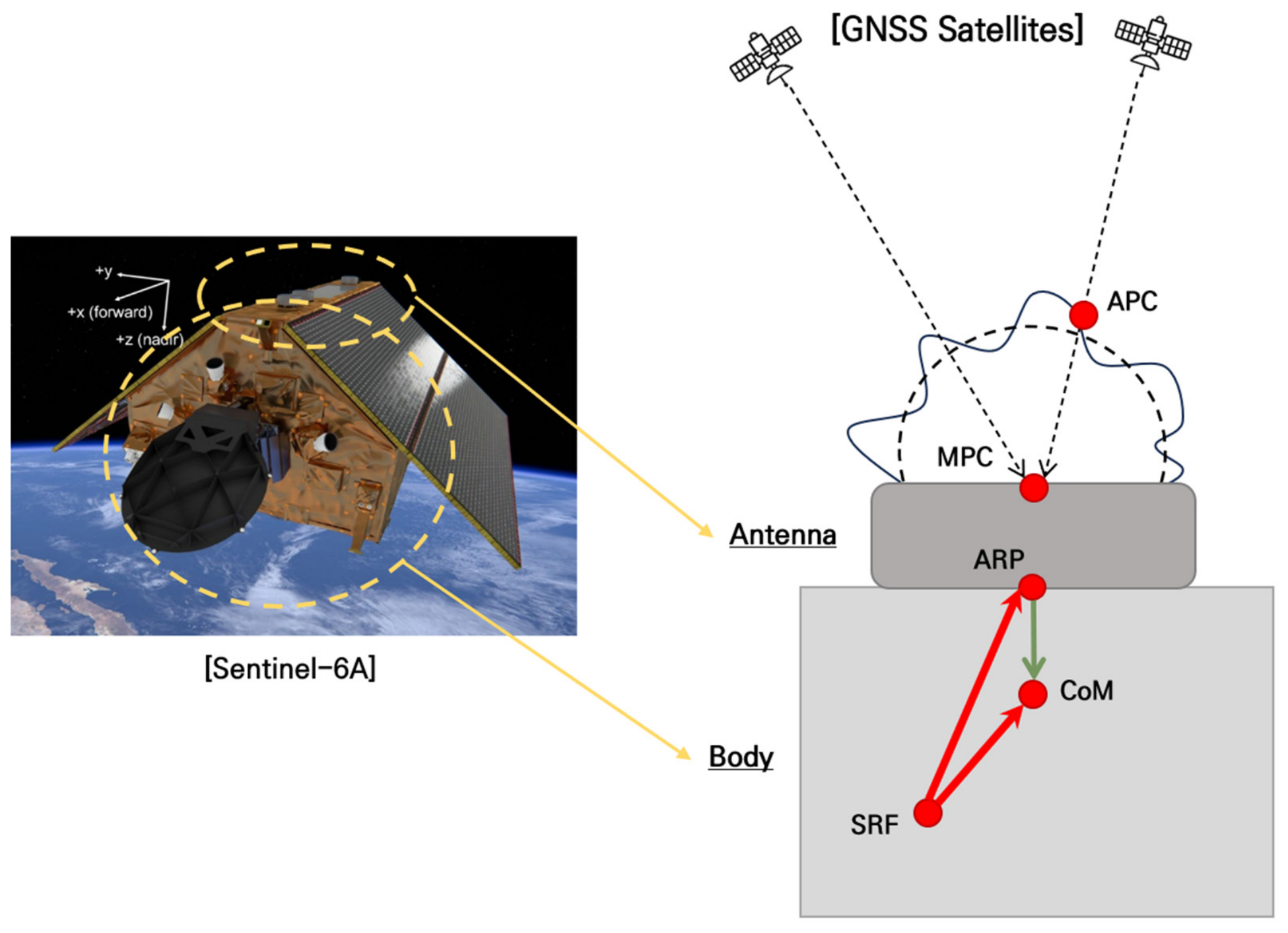
For the Sentinel-6A satellite, coordinates directly estimated from GNSS observations are defined with respect to the Antenna Phase Center (APC) or Mean Phase Center (MPC), while the reference coordinates provided by the SP3 product are defined relative to the satellite’s Center of Mass (CoM). Therefore, a fixed offset exists between these reference points due to the geometric structure of the satellite, which, if not properly accounted for, may introduce bias in the orbit error assessment.
In this study, for comparison with the SP3 reference coordinates, the Antenna Reference Point (ARP) was adopted as the reference point for the estimated coordinates instead of the APC or MPC, and only the transformation from ARP to CoM was applied. In other words, Phase Center Offset (PCO) and Phase Center Variation (PCV) corrections from the ARP to the antenna phase center were not applied, and only the geometric transformation between the ARP and CoM was considered to ensure comparability with the reference orbit. The ARP and CoM coordinates, defined in the Satellite Reference Frame (SRF), are taken from [44] and listed in Table 2.
Table 2.
ARP and CoM coordinates of Sentinel-6A expressed in the SRF. The coordinates are adopted from [44] and used to define the geometric offset between the ARP and CoM for the coordinate correction.
Since all coordinates in Table 2 are defined in the SRF, they must be transformed into the Earth-centered Earth-fixed (ECEF) frame for position comparison and error analysis. In this study, a two-step rotation transformation is applied. First, using satellite attitude information, the transformation from the SRF to the Earth-Centered Inertial (ECI) frame is performed. Subsequently, the transformation from ECI to ECEF is carried out by accounting for Earth’s rotation. The transformation from SRF to ECI is performed using a rotation matrix derived from the satellite attitude quaternion, as shown in Equation (9).
Here, , , , and denote the components of the quaternion representing satellite attitude. The attitude quaternion data are obtained from the Sentinel-6A attitude products provided by CDSE. The transformation from ECI to ECEF is performed using a z-axis rotation matrix based on the Greenwich sidereal time , as given in Equation (10).
The two rotation matrices introduced above are sequentially applied to transform the SRF reference vector into the ECEF coordinate system. To define the geometric offset between the ARP and the CoM, the position vectors to the ARP and CoM in the SRF are denoted by and , respectively. The difference between these vectors defines the CoM-to-ARP vector (CAV), as expressed in Equation (11). The CAV is a fixed vector representing the relative position of the ARP with respect to the CoM in the SRF. The defined is then transformed into the ECEF frame by sequentially applying the rotation matrices given in Equations (9) and (10). The corresponding formulation is presented in Equation (12).
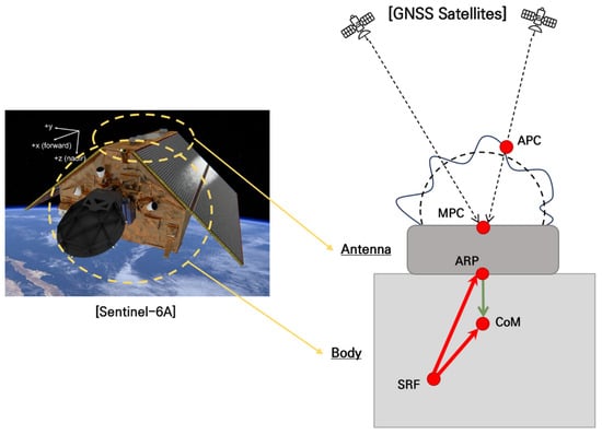
The transformed vector is projected onto the LOS unit vector from the satellite to the receiver to obtain the corresponding pseudorange correction. The correction value is computed as the dot product between the LOS unit vector and , as given in Equation (13). The coordinate transformation and vector projection procedures are illustrated in Figure 1.
Figure 1.
Coordinate correction process from the ARP to the CoM. The green arrow represents the CAV in the SRF, which is transformed into the ECEF frame and projected onto the LOS vector to derive the pseudorange correction. The red arrows indicate the vectors from the SRF origin to the ARP and from the SRF origin to the CoM, respectively.
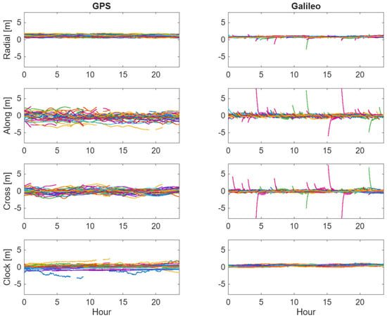
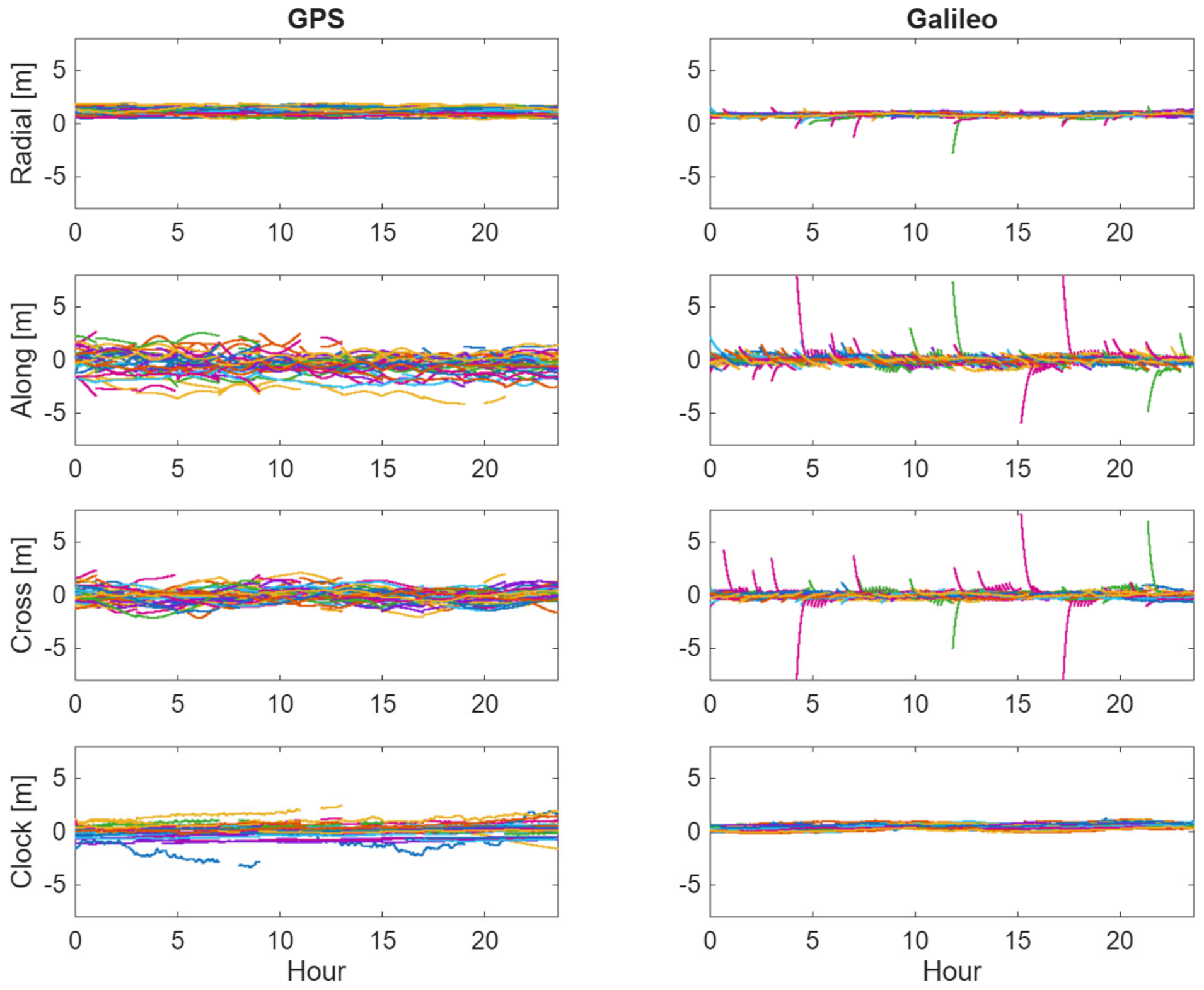
To calculate the SISRE-based weighting coefficients described in Section 2, the accuracy of broadcast ephemerides was evaluated by comparison with precise orbit and clock products for Galileo and GPS satellites on 10 August 2023. The broadcast ephemerides for the GNSS satellites were collected from CDDIS, and the precise orbit and clock products were also obtained from the SP3 files provided by CDDIS. Additionally, the antenna correction model provided by the International GNSS Service (IGS) was applied for PCO correction. The evaluation was conducted by comparing satellite positions and clock offsets at common epochs, enabling quantitative assessment of the orbit and clock error characteristics of the broadcast ephemerides. The differences between the broadcast ephemerides and precise orbit products are presented as time series in Figure 2, and the corresponding RMSE and SISRE values for radial, along-track, cross-track, and clock errors by satellite constellation are summarized in Table 3.
Figure 2.
Errors in GPS and Galileo broadcast ephemerides relative to the precise orbit and clock products on 10 August 2023.
Table 3.
RMSE values in the radial, along-track, and cross-track directions and signal-in-space range errors of the broadcast ephemerides relative to the precise orbit and clock products.
As shown in Figure 2, relatively large orbit differences are observed for Galileo immediately after newly updated broadcast ephemeris parameters are applied. This is because the newly updated ephemeris represents a new prediction arc based on updated navigation information, and its initial consistency with the precise orbit products is generally lower than that achieved toward the end of the previous arc. Within the same ephemeris arc, these differences tend to gradually decrease as the predicted broadcast orbit becomes more consistent with the precise orbit products. Table 3 summarizes these errors in terms of RMSE and the corresponding SISRE values.
The SISRE-based weighting coefficients were computed by normalizing the weights of the Galileo satellites, which exhibit smaller SISRE values, to unity and expressing the weights of the GPS satellites as relative values with respect to those of Galileo. Based on the SISRE values obtained in this study, the resulting relative weighting ratio was approximately 1:0.174. In a strict real-time orbit determination scenario, however, SISRE values cannot be directly computed for the current day because precise reference orbit and clock products are not available in real time. Therefore, to examine whether the SISRE coefficient obtained on the validation day is representative of recently available SISRE information, the SISRE values of GPS and Galileo broadcast ephemerides were additionally evaluated over approximately two weeks preceding the validation day and summarized in Table 4.
Table 4.
Daily RMSE values in the radial, along-track, cross-track, and clock components, and corresponding SISRE values of the broadcast ephemerides relative to precise orbit and clock products during the two-week period preceding the validation day.
As summarized in Table 4, GPS SISRE remained within approximately 0.49–0.62 m, while Galileo SISRE remained within approximately 0.23–0.28 m. Accordingly, the relative GPS weighting coefficient with respect to Galileo remained within a similar range, generally around 0.2.
These results indicate that the SISRE-based coefficients used in the main validation are consistent with the recent SISRE trend, rather than being values specific to a single day. Thus, in practical real-time implementation, the SISRE-based coefficients do not need to be estimated epoch by epoch during real-time processing. Instead, they can be precomputed using the most recently available orbit and clock products, such as previous-day or recent reference-period statistics, and then applied as constellation-level weights.
3. Results
3.1. Orbit Determination Performance
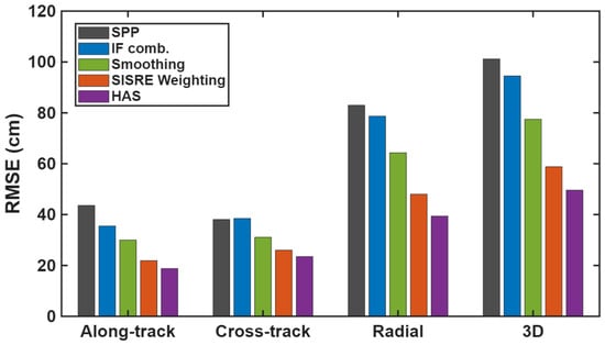
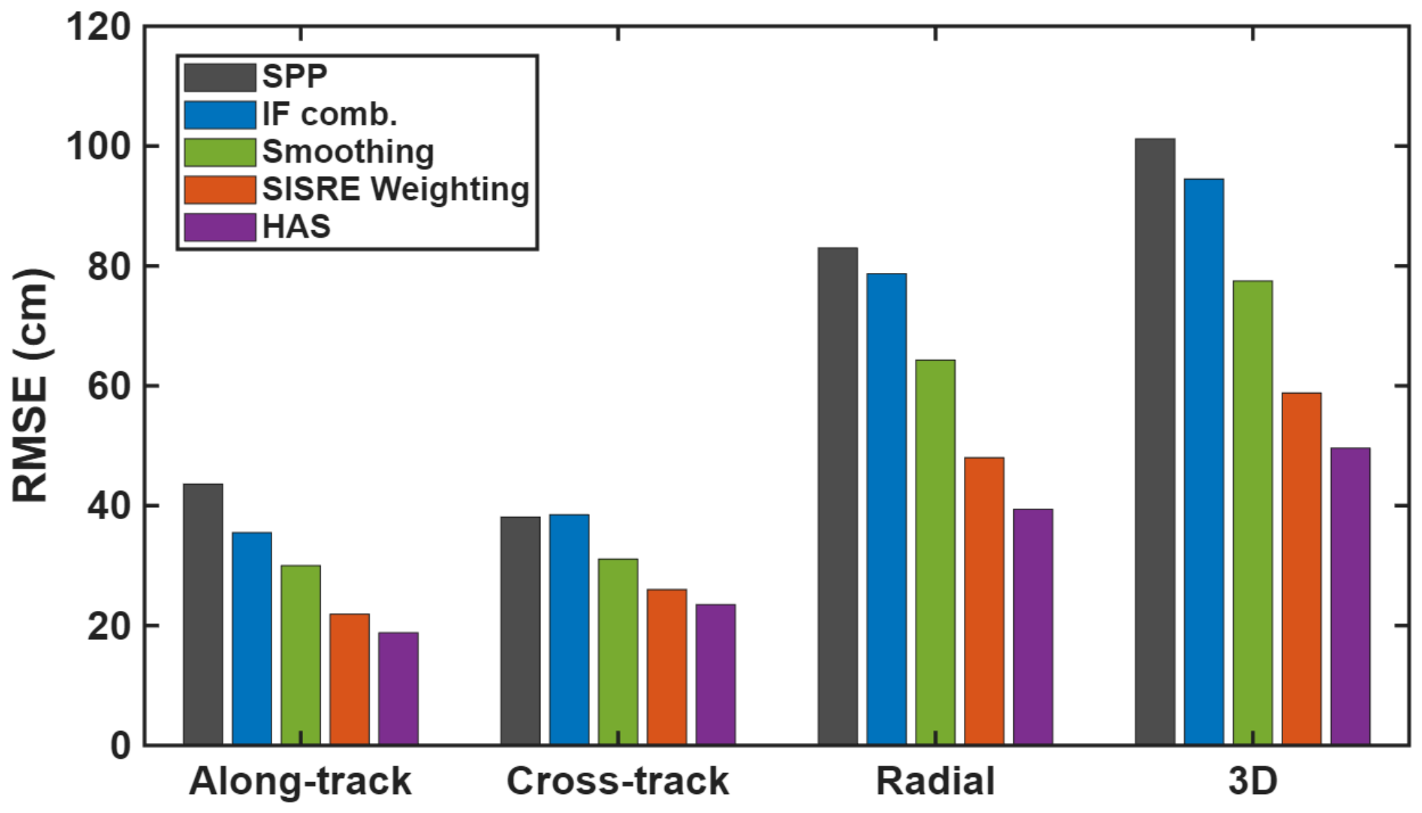
In this section, the performance of the proposed orbit determination method is quantitatively evaluated by comparison with SP3 precise orbit products. The RMSE values of the radial, along-track, cross-track, and 3D errors obtained by cumulatively applying the processing techniques described in Section 2 are summarized in Table 5 and illustrated in Figure 3. Here, Standard Point Positioning (SPP) denotes the orbit determination solution based solely on single-frequency code pseudorange measurements, without applying ionospheric correction, code–carrier smoothing, or satellite orbit and clock corrections.
Table 5.
RMSE of radial, along-track, cross-track, and 3D components for each processing configuration. Each “+” indicates the cumulative addition of the corresponding processing technique to the previous solution, starting from the SPP.
Figure 3.
Bar chart representation of the RMSE values listed in Table 5 for the radial, along-track, cross-track, and 3D components under each processing strategy.
The 3D RMSE of the SPP solution was 101.2 cm, indicating that meter-level orbit accuracy was achieved. As the processing techniques described in Section 2 were cumulatively applied, a progressive reduction in RMSE was observed. With the application of the dual-frequency IF combination, the 3D RMSE decreased to 94.5 cm, corresponding to an improvement of approximately 6.6%. However, the radial component remained the dominant error source, with an RMSE of 78.7 cm. This was attributed to the residual effects of code noise amplification and remaining errors, despite the mitigation of the first-order ionospheric delay. After applying code–carrier smoothing, a significant reduction in RMSE was observed in all components, owing to reduced code noise. Furthermore, by applying the SISRE-based robust weighting model, different weights were assigned to the observations based on the orbit and clock accuracies of each GNSS system, leading to additional accuracy improvement. Finally, when HAS corrections were applied, the 3D RMSE was reduced to 49.6 cm, achieving an improvement of approximately 51% compared to the SPP solution.
3.2. Mean Error and Time-Series Characteristics
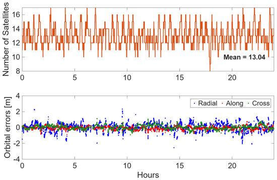
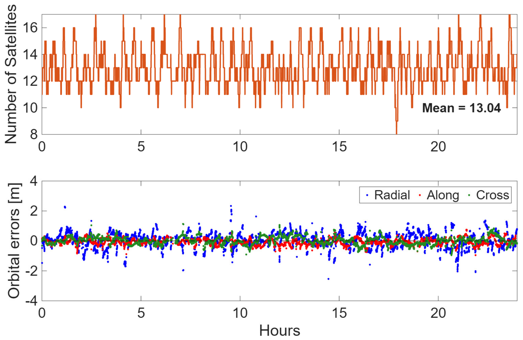
In addition, the mean errors of the radial, along-track and cross-track components are summarized in Table 6. The radial mean error of the SPP solution exhibited the largest bias among the three components, indicating the presence of a significant systematic bias in the radial component. After applying the IF combination, the radial mean error was significantly reduced to 7.9 cm, demonstrating that the removal of the first-order ionospheric delay contributed directly to bias mitigation in the radial component. The along-track and cross-track mean errors also showed slight reductions. Following the application of code-carrier smoothing, the radial mean error decreased to below 5 cm, suggesting that not only random noise but also part of the bias component was mitigated. After applying the SISRE-based weighting, the mean errors in all directional components were reduced to below 5 cm. Although HAS corrections slightly increased cross-track errors, they remained at centimeter level with negligible impact on overall accuracy. Figure 4 shows time-series variations in radial, along-track, and cross-track errors for the HAS-corrected final solution, along with satellite numbers.
Table 6.
Mean errors in radial, along-track and cross-track components for each processing strategy.
Figure 4.
Time series of the radial, along-track, and cross-track orbit errors and the number of satellites. The blue, red, and green markers represent the radial, along-track, and cross-track errors, respectively.
4. Discussion
4.1. Remaining Error Sources
As shown in Figure 4, approximately 13 satellites were used on average during the test period. The radial error is the largest among the three directional components. This can be attributed to the fact that the PCO and PCV corrections between the ARP and the antenna phase center were not considered, and only the first-order ionospheric delay was removed. The radial component, represented by the blue markers, corresponds to the direction between the LEO satellite and the Earth’s center and is therefore most directly affected by residual errors in the pseudorange observations. In particular, higher-order ionospheric delay terms are not completely eliminated and remain as residuals, which are primarily projected onto the range component and contribute to increased radial errors [45]. In addition, residual errors from satellite clock estimation are directly reflected in pseudorange observations. Since these clock errors are geometrically coupled with the range component in the observation model, they may exhibit some correlation with radial errors [46]. Consequently, imperfections in clock error estimation may also contribute to the observed increase in the radial error.
4.2. Temporal Behavior and Satellite Visibility
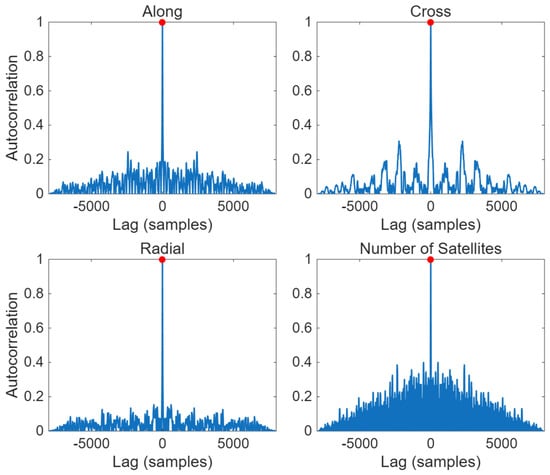
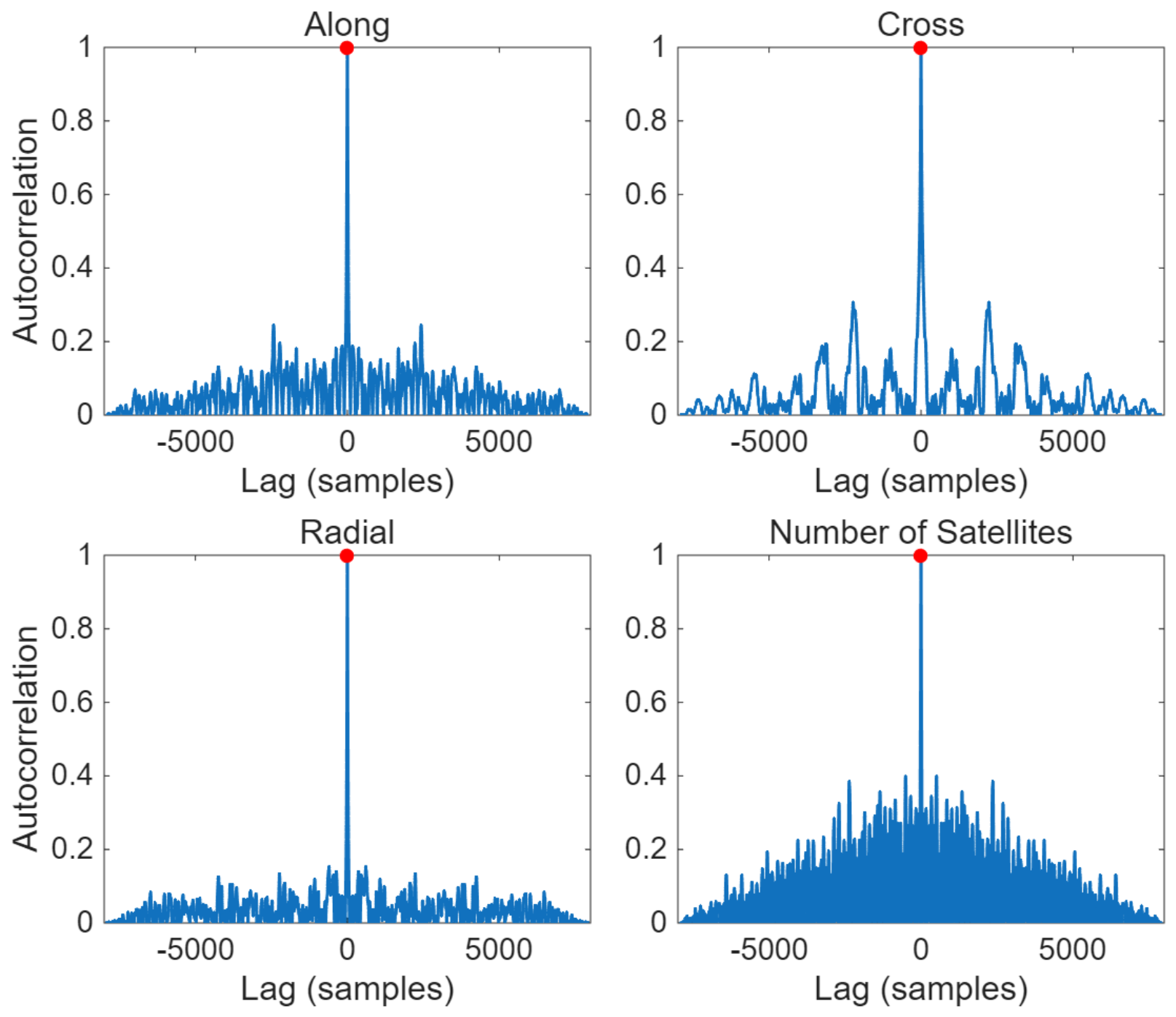
The temporal variations in directional errors and the number of satellites suggest a periodic pattern. To investigate this, the autocorrelation function (ACF) was computed for each component, and the results are shown in Figure 5. As shown in Figure 5, the autocorrelation values for the along-track, cross-track, and radial errors, as well as the number of satellites, reach their maximum at zero lag. For non-zero lags, however, the autocorrelation values remain low and irregularly distributed, with no distinct periodic peaks observed.
Figure 5.
Autocorrelation analysis of orbit errors in the along-track, cross-track, and radial directions, along with the number of satellites. The red circles indicate the points at which the autocorrelation reaches its maximum value.
The autocorrelation analysis shows that the along-track and radial errors exhibit minimal temporal correlation, indicating predominantly noise-like behavior. In contrast, the cross-track errors show relatively larger correlations at non-zero lags among the three components, which is consistent with the more pronounced periodic pattern observed in Figure 4. However, the magnitude of these correlations is still limited, indicating that the periodicity is not sufficiently strong to be considered significant. Meanwhile, the number of satellites demonstrates strong temporal correlation, reflecting slowly varying satellite visibility and orbital geometry. These results indicate that most of the remaining orbit errors are largely uncorrelated over time, with only minor structured components observed in the cross-track direction.
The autocorrelation results indicate that the analyzed orbit errors are dominated by stochastic components that vary irregularly over time, rather than systematic errors with distinct periodicity. In addition, a correlation analysis between the 3D orbit error and the number of satellites was performed. The resulting correlation coefficient of 0.033 indicates a negligible relationship between the 3D orbit error and the number of satellites.
4.3. Spatial Characteristics and HAS Regional Dependence
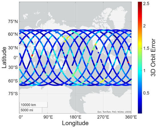
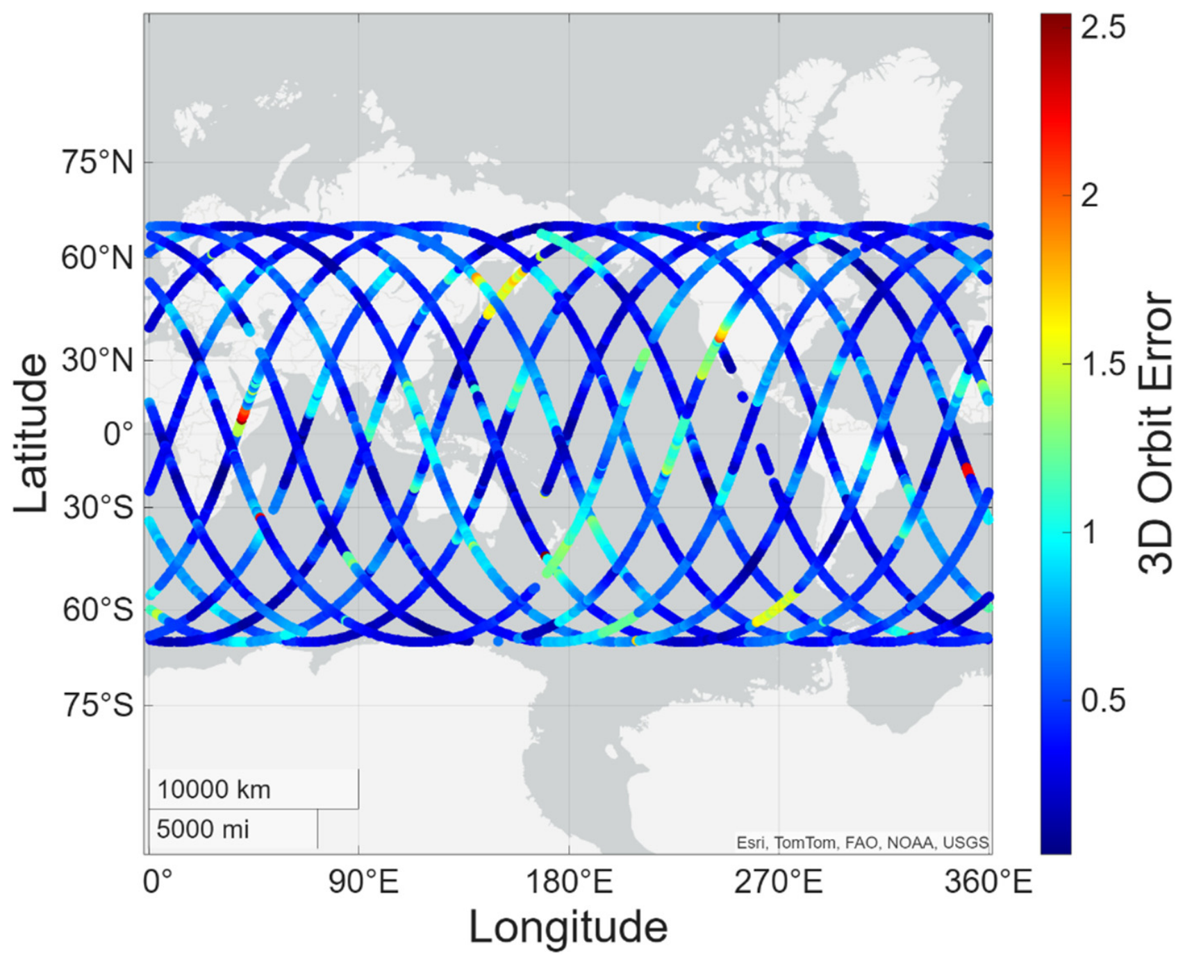
To further investigate the potential impact of satellite ground track variations on the observed error behavior, the relationship between the satellite ground track and the 3D orbit error was analyzed. The 3D error was projected onto the ground track, and the results are shown in Figure 6. As shown in Figure 6, no distinct spatial pattern was observed, with orbit errors showing no consistent increase or decrease over specific latitudinal or longitudinal regions along the satellite trajectory. Although relatively large errors appeared in certain segments, these were not concentrated in particular geographic regions but distributed across the entire ground track. These findings suggest that the magnitude of the 3D orbit error is not directly related to the satellite’s geographic location and that the proposed method provides stable performance without regional bias.
Figure 6.
Projection of 3D orbit errors onto the satellite ground track, illustrating the spatial distribution of orbit errors along the satellite trajectory. The color bar indicates the magnitude of the 3D orbit error, with red representing larger errors and blue representing smaller errors.
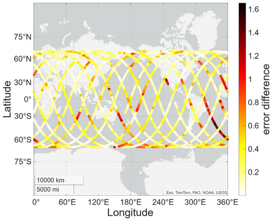
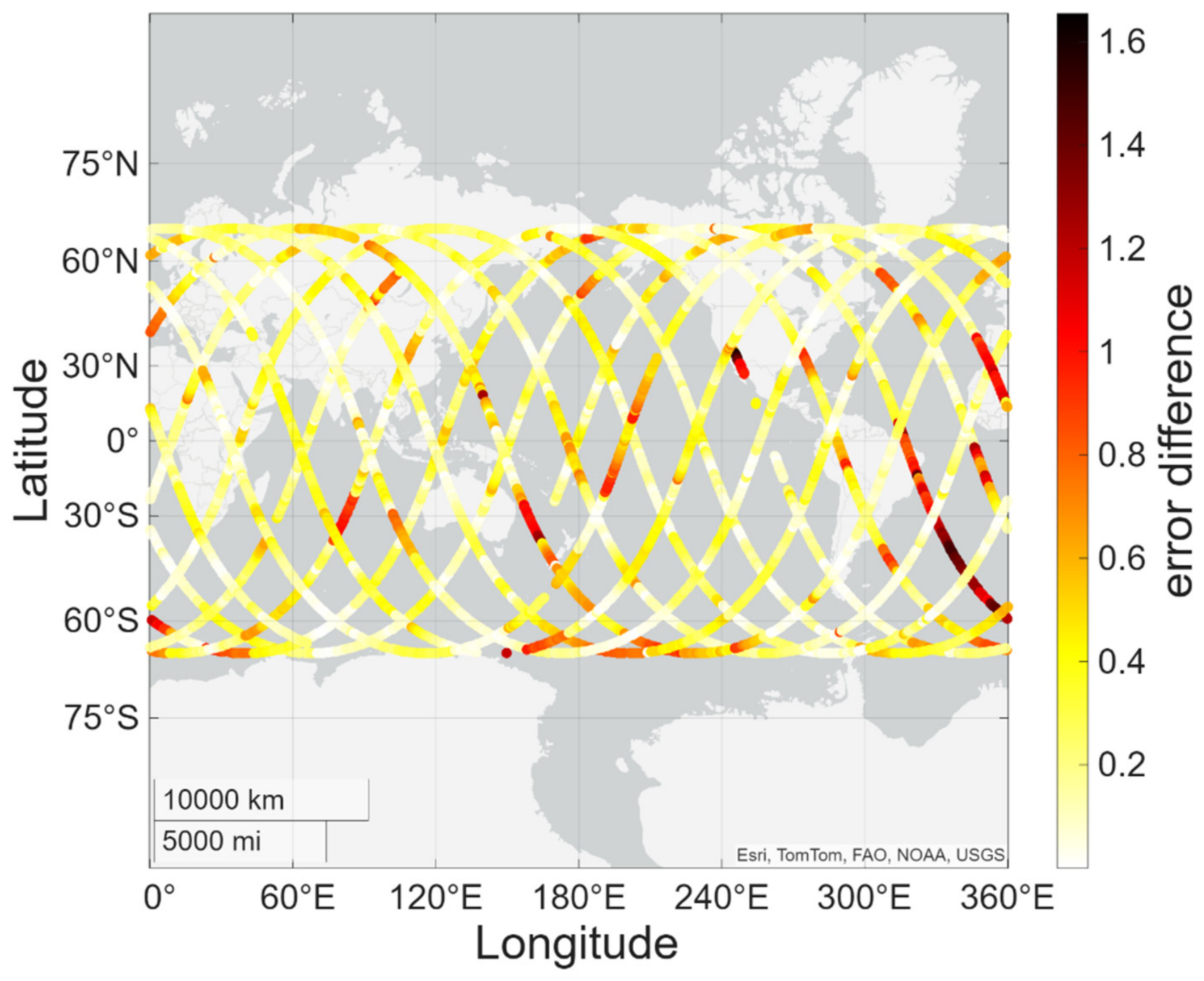
Since the performance of HAS corrections can be influenced by the distribution of Galileo ground infrastructure, their effectiveness may vary regionally, particularly in areas outside Europe, including Asia and the Pacific [47,48]. Ref. [49] analyzed HAS-based PPP performance over a six-day period using 10 receivers located in Europe, Africa, the Americas, the Pacific, and Asia. The results showed that the HAS-based PPP solutions satisfied the horizontal and vertical 95% accuracy criteria in Europe and Africa. In contrast, performance degradation was identified in the Americas and Asia. As shown in Table 5, the application of HAS corrections reduced the overall 3D RMSE to 49.6 cm, indicating a noticeable improvement in orbit accuracy. To further examine the spatial characteristics of this improvement, the change in 3D orbit error due to HAS corrections was projected onto the satellite ground track, as shown in Figure 7.
Figure 7.
Projection of differences in 3D orbit errors before and after HAS corrections onto the satellite ground track. The color bar represents the magnitude of the error difference, with darker red and lighter yellow colors indicating larger and smaller differences, respectively.
As illustrated in Figure 7, the application of HAS corrections generally contributed to an improvement in orbit accuracy, with error differences remaining relatively uniform and below 0.4 m over most segments of the ground track. However, in the segment passing near the Atlantic Ocean, larger changes in the 3D orbit error were observed. This may result from higher-quality correction data near Europe, where Galileo Sensor Stations are more densely distributed than in the Asia-Pacific region [50]. These regional variations indicate that HAS correction performance is not globally uniform and that its effectiveness depends on factors such as the distribution of ground stations.
5. Conclusions
This study introduced a kinematic orbit determination approach for LEO satellites based on code pseudorange observations, without relying on dynamic models or carrier-phase-based integer ambiguity resolution. In the proposed algorithm, a dual-frequency IF combination, code–carrier smoothing, an SISRE-based robust weighting model, and HAS corrections were applied in real time. The algorithm was validated using Sentinel-6A data, and its performance was assessed through comparison with SP3 precise orbit products. The validation results showed that the 3D RMSE of the SPP solution was 101.2 cm and decreased to 49.6 cm after applying the correction techniques, representing a reduction of approximately 51%. In particular, the along-track component showed the largest improvement of approximately 57%. The radial bias dropped from 52.7 cm to 1.4 cm (a 97% decrease), while the along-track and cross-track components also exhibited consistent reductions. These results demonstrate that real-time LEO kinematic orbit determination with sub-meter accuracy can be achieved based on code pseudorange observations, confirming its feasibility for various LEO-based PNT applications.
Author Contributions
Conceptualization, H.-S.L. and K.-D.P.; methodology, H.-S.L.; software, H.-S.L.; validation, H.-S.L.; formal analysis, H.-S.L. and K.-D.P.; investigation, H.-S.L.; resources, H.-S.L. and K.-D.P.; data curation, H.-S.L.; writing—original draft preparation, H.-S.L.; writing—review and editing, H.-S.L. and K.-D.P.; visualization, H.-S.L.; supervision, K.-D.P.; project administration, K.-D.P.; funding acquisition, K.-D.P. All authors have read and agreed to the published version of the manuscript.
Funding
This work is supported by the Korea Agency for Infrastructure Technology Advancement grant funded by the Ministry of Land, Infrastructure and Transport (RS-2022-00141819, Development of Advanced Technology for Absolute, Relative, and Continuous Complex Positioning to Acquire Ultra-precise Digital Land Information).
Data Availability Statement
The data generated in this study are available from the corresponding author upon reasonable request.
Conflicts of Interest
Author Kwan-Dong Park was employed by the company PPSOL Inc. The authors declare that the research was conducted in the absence of any commercial or financial relationships that could be construed as a potential conflict of interest.
Abbreviations
| LEO | low Earth orbit |
| GNSS | Global Navigation Satellite Systems |
| PNT | Positioning, Navigation, and Timing |
| SNR | Signal-to-Noise Ratio |
| DOD | Dynamic Orbit Determination |
| RDOD | Reduced-Dynamic Orbit Determination |
| KOD | Kinematic Orbit Determination |
| LOS | Line-of-Sight |
| PCA | Piecewise Constant Acceleration |
| RMSE | Root Mean Square Error |
| AR | Ambiguity Resolution |
| GRAPHIC | Group and Phase Ionospheric Correction |
| IF | Ionosphere-Free |
| SISRE | Signal-in-Space Range Error |
| HAS | High Accuracy Service |
| LLI | Loss of Lock Indicator |
| UERE | User Equivalent Range Error |
| DOP | Dilution of Precision |
| UEE | User Equipment Error |
| GES DISC | Goddard Earth Sciences Data and Information Services Center |
| CDDIS | Crustal Dynamics Data Information System |
| SP3 | Standard Product 3 |
| CDSE | Copernicus Data Space Ecosystem |
| BKG | Bundesamt für Kartographie und Geodäsie |
| BNC | BKG Ntrip Client |
| APC | Antenna Phase Center |
| MPC | Mean Phase Center |
| CoM | Center of Mass |
| ARP | Antenna Reference Point |
| PCO | Phase Center Offset |
| PCV | Phase Center Variation |
| SRF | Satellite Reference Frame |
| ECEF | Earth-Centered, Earth-Fixed |
| ECI | Earth-Centered Inertial |
| CAV | CoM-to-ARP Vector |
| IGS | International GNSS Service |
| SPP | Standard Point Positioning |
| ACF | Autocorrelation Function |
References
- Benzerrouk, H.; Nguyen, Q.; Xiaoxing, F.; Amrhar, A.; Nebylov, A.V.; Landry, R. Alternative PNT based on iridium Next LEO satellites Doppler/INS integrated navigation system. In 2019 26th Saint Petersburg International Conference on Integrated Navigation Systems (ICINS); IEEE: New York, NY, USA, 2019; pp. 1–10. [Google Scholar] [CrossRef] [Scilit]
- Nardin, A.; Dovis, F.; Fraire, J.A. Empowering the tracking performance of LEO PNT by means of meta-signals. In 2020 IEEE International Conference on Wireless for Space and Extreme Environments (WiSEE); IEEE: New York, NY, USA, 2020; pp. 153–158. [Google Scholar] [CrossRef] [Scilit]
- Egea-Roca, D.; López-Salcedo, J.A.; Seco-Granados, G.; Falletti, E. Comparison of several signal designs based on chirp spread spectrum (CSS) modulation for a LEO PNT system. In Proceedings of the ION GNSS+, the International Technical Meeting of the Satellite Division of the Institute of Navigation, St. Louis, MO, USA, 20–24 September 2021; pp. 2804–2818. [Google Scholar] [CrossRef] [Scilit]
- Yang, Y.; Mao, Y.; Ren, X.; Jia, X.; Sun, B. Demand and key technology for a LEO constellation as augmentation of satellite navigation systems. Satell. Navig. 2024, 5, 11. [Google Scholar] [CrossRef] [Scilit]
- Deng, R.; Qin, H.; Zhang, Y. Non-cooperative LEO satellite orbit determination using single station for space-based opportunistic positioning. Remote Sens. 2024, 16, 912. [Google Scholar] [CrossRef] [Scilit]
- Tapley, B.D. Fundamentals of orbit determination. In Theory of Satellite Geodesy and Gravity Field Determination; Sansò, F., Rummel, R., Eds.; Springer: Berlin/Heidelberg, Germany, 1989; pp. 235–260. [Google Scholar] [CrossRef] [Scilit]
- Frontier SI. State of the Market Report: Low Earth Orbit Positioning, Navigation and Timing (LEO PNT), 2024 ed. (v1.1); Frontier SI: Victoria, Australia, 2024. [Google Scholar]
- Švehla, D.; Rothacher, M. Kinematic and reduced-dynamic precise orbit determination of low Earth orbiters. Adv. Geosci. 2003, 1, 47–56. [Google Scholar] [CrossRef] [Scilit]
- Mur, T.J.M.; Dow, J.M. Satellite Navigation Using GPS; ESA Bulletin Nr. 90. 1997. Available online: https://www.esa.int/esapub/bulletin/bullet90/b90mur.htm (accessed on 3 June 2026).
- Selvan, K.; Siemuri, A.; Prol, F.S.; Välisuo, P.; Bhuiyan, M.Z.H.; Kuusniemi, H. Precise orbit determination of LEO satellites: A systematic review. GPS Solut. 2023, 27, 178. [Google Scholar] [CrossRef] [Scilit]
- Wu, S.C.; Yunck, T.P.; Thornton, C.L. Reduced-dynamic technique for precise orbit determination of low Earth satellites. J. Guid. Control Dyn. 1991, 14, 24–30. [Google Scholar] [CrossRef] [Scilit] [PubMed]
- Montenbruck, O.; van Helleputte, T.; Kroes, R.; Gill, E. Reduced dynamic orbit determination using GPS code and carrier measurements. Aerosp. Sci. Technol. 2005, 9, 261–271. [Google Scholar] [CrossRef] [Scilit]
- Hauschild, A.; Montenbruck, O. Precise real-time navigation of LEO satellites using GNSS broadcast ephemerides. Navigation 2021, 68, 419–432. [Google Scholar] [CrossRef] [Scilit]
- Montenbruck, O.; Kunzi, F.; Hauschild, A. Performance assessment of GNSS-based real-time navigation for the Sentinel-6 spacecraft. GPS Solut. 2021, 26, 12. [Google Scholar] [CrossRef] [Scilit]
- Wang, F.; Gong, X.; Sang, J.; Zhang, X. A novel method for precise onboard real-time orbit determination with a standalone GPS receiver. Sensors 2015, 15, 30403–30418. [Google Scholar] [CrossRef] [Scilit] [PubMed]
- Swatschina, P. Dynamic and Reduced-Dynamic Precise Orbit Determination of Satellites in Low Earth Orbits. Ph.D. Thesis, Vienna University of Technology, Vienna, Austria, 2012. [Google Scholar]
- Yang, Y.; Yue, X.; Dempster, A.G. GPS-based onboard real-time orbit determination for LEO satellites using consider Kalman filter. IEEE Trans. Aerosp. Electron. Syst. 2016, 52, 769–777. [Google Scholar] [CrossRef] [Scilit]
- Wang, Z.; Li, Z.; Wang, N.; Hoque, M.; Wang, L.; Li, R.; Zhang, Y.; Yuan, H. Real-time precise orbit determination for LEO between kinematic and reduced-dynamic with ambiguity resolution. Aerospace 2022, 9, 25. [Google Scholar] [CrossRef] [Scilit]
- Allahvirdi-Zadeh, A.; Wang, K.; El-Mowafy, A. Precise orbit determination of LEO satellites based on undifferenced GNSS observations. J. Surv. Eng. 2022, 148, 03121001. [Google Scholar] [CrossRef] [Scilit]
- Zelensky, N.P.; Lemoine, F.G.; Ziebart, M.; Sibthorpe, A.; Willis, P.; Beckley, B.D.; Klosko, S.M.; Chinn, D.S.; Rowlands, D.D.; Luthcke, S.B.; et al. DORIS/SLR POD modeling improvements for Jason-1 and Jason-2. Adv. Space Res. 2010, 46, 1541–1558. [Google Scholar] [CrossRef] [Scilit]
- Allende-Alba, G.; Montenbruck, O.; Ardaens, J.S.; Wermuth, M.; Hugentobler, U. Estimating maneuvers for precise relative orbit determination using GPS. Adv. Space Res. 2017, 59, 45–62. [Google Scholar] [CrossRef] [Scilit]
- Peng, D.; Wu, B. Kinematic precise orbit determination for LEO satellites using space-borne dual-frequency GPS measurements. Chin. Astron. Astrophys. 2012, 36, 291–306. [Google Scholar]
- Weinbach, U.; Schön, S. Improved GRACE kinematic orbit determination using GPS receiver clock modeling. GPS Solut. 2012, 17, 511–520. [Google Scholar] [CrossRef] [Scilit]
- Zehentner, N.; Mayer-Gürr, T. Precise orbit determination based on raw GPS measurements. J. Geod. 2015, 90, 275–286. [Google Scholar] [CrossRef] [Scilit]
- Chen, P.; Zhang, J.; Sun, X. Real-time kinematic positioning of LEO satellites using a single-frequency GPS receiver. GPS Solut. 2016, 21, 973–984. [Google Scholar] [CrossRef] [Scilit]
- Li, X.; Wu, J.; Zhang, K.; Li, X.; Xiong, Y.; Zhang, Q. Real-time kinematic precise orbit determination for LEO satellites using zero-differenced ambiguity resolution. Remote Sens. 2019, 11, 2815. [Google Scholar] [CrossRef] [Scilit]
- Gong, X.; Sang, J.; Wang, F.; Li, X. LEO onboard real-time orbit determination using GPS/BDS data with an optimal stochastic model. Remote Sens. 2020, 12, 3458. [Google Scholar] [CrossRef] [Scilit]
- Fu, W.; Wang, L.; Chen, R.; Zhou, H.; Li, T.; Han, Y. Improved single-frequency kinematic orbit determination strategy of small LEO satellite with the sun-pointing attitude mode. Remote Sens. 2021, 13, 4020. [Google Scholar] [CrossRef] [Scilit]
- Misra, P.; Enge, P. Global Positioning System: Signals, Measurements, and Performance, 2nd ed.; Ganga-Jumana Press: Lincoln, MA, USA, 2012. [Google Scholar]
- Kouba, J.; Héroux, P. Precise point positioning using IGS orbit and clock products. GPS Solut. 2001, 5, 12–28. [Google Scholar] [CrossRef] [Scilit]
- Odijk, D. Ionosphere-free phase combinations for modernized GPS. J. Surv. Eng. 2003, 129, 165–173. [Google Scholar] [CrossRef] [Scilit]
- Petovello, M.; van der Marel, H.; de Bakker, P.F. Single versus dual frequency precise point positioning. Inside GNSS 2012, 7, 30–35. [Google Scholar]
- Zhou, Z.; Li, B. Optimal Doppler-aided smoothing strategy for GNSS navigation. GPS Solut. 2017, 21, 197–210. [Google Scholar] [CrossRef] [Scilit]
- Petovello, M.; Lo Presti, L.; Visintin, M. Can you list all the properties of the carrier-smoothing filter? Inside GNSS 2015, 10, 32–37. [Google Scholar]
- Jiang, N.; Cao, Y.; Xia, F.; Huang, H.; Meng, Y.; Zhou, S.; Qu, W.; Hu, X. Broadcast ephemeris SISRE assessment and systematic error characteristic analysis for BDS and GPS satellite systems. Adv. Space Res. 2024, 73, 5284–5298. [Google Scholar] [CrossRef] [Scilit]
- Chen, L.; Jiao, W.; Huang, X.; Geng, C.; Ai, L.; Lu, L.; Hu, Z. Study on signal-in-space errors calculation method and statistical characterization of BeiDou navigation satellite system. In China Satellite Navigation Conference (CSNC) 2013 Proceedings; Sun, J., Jiao, W., Wu, H., Shi, C., Eds.; Springer: Berlin/Heidelberg, Germany, 2013; pp. 423–434. [Google Scholar] [CrossRef] [Scilit]
- Warren, D.L.; Raquet, J.F. Broadcast vs. precise GPS ephemerides: A historical perspective. GPS Solut. 2003, 7, 151–156. [Google Scholar] [CrossRef] [Scilit]
- Heng, L.; Gao, G.X.; Walter, T.; Enge, P. Statistical characterization of GPS signal-in-space errors. In Proceedings of the Ion ITM, San Diego, CA, USA, 24–26 January 2011; pp. 312–319. [Google Scholar]
- Rodriguez, R.L. Galileo IOV status and results. In Proceedings of the Ion GNSS, Nashville, TN, USA, 16–20 September 2013; pp. 3065–3093. [Google Scholar]
- Yang, J.H.; Tang, C.P.; Song, Y.Z.; Hu, X.; Zhou, S.; Chang, Z. Analysis of signal-in-space ranging error of GNSS navigation message. Sci. China Phys. Mech. Astron. 2021, 51, 019508. [Google Scholar]
- Huber, P.J. Robust estimation of a location parameter. Ann. Math. Stat. 1964, 35, 492–518. [Google Scholar] [CrossRef] [Scilit]
- Han, W.S.; Park, K.D. Comparison of Galileo HAS and IGS RTS corrections and development of a Galileo HAS based GNSS positioning algorithm. J. Position Navig. Timing 2024, 13, 431–439. [Google Scholar]
- Angrisano, A.; Ascione, S.; Cappello, G.; Gioia, C.; Gaglione, S. Application of “Galileo high accuracy service” on single-point positioning. Sensors 2023, 23, 4223. [Google Scholar] [CrossRef] [Scilit] [PubMed]
- ESA. Sentinel-6 Michael Freilich POD Context (JC-TN-ESA-SY-0420). Sentinel Online, 2023. Available online: https://ids-doris.org/documents/BC/satellites/Sentinel6A_PODcontext.pdf (accessed on 3 June 2026).
- Liu, Z.; Li, Y.; Guo, J.; Li, F. Influence of higher-order ionospheric delay correction on GPS precise orbit determination and precise positioning. Geod. Geodyn. 2016, 7, 369–376. [Google Scholar] [CrossRef] [Scilit]
- Johnston, G.; Riddell, A.; Hausler, G. The International GNSS Service. In Springer Handbook of Global Navigation Satellite Systems; Springer: Berlin/Heidelberg, Germany, 2017. [Google Scholar]
- Ren, X.; Yang, H.; Xu, G.; Yao, K.; Zhang, Y.; Zhang, X. Galileo HAS compared with WHU RTS. Adv. Space Res. 2025, 76, 3291–3304. [Google Scholar] [CrossRef] [Scilit]
- EUSPA. Galileo HAS Service Definition Document; EUSPA: Prague, Czech Republic, 2023.
- Chamorro, A.; Cancela, S.; García, A.J.; Calle, D.; Fernández-Hernández, I.; de Blas, F.J.; Vazquez, J.; Hernández, C. Early demonstration of Galileo HAS user performances. In Proceedings of the Ion GNSS, Denver, CO, USA, 19–23 September 2022; pp. 828–835. [Google Scholar] [CrossRef] [Scilit]
- Fernandez-Hernandez, I.; Chamorro-Moreno, A.; Cancela-Diaz, S.; Calle-Calle, J.D.; Zoccarato, P.; Blonski, D.; Senni, T.; de Blas, F.J.; Hernández, C.; Simón, J.; et al. Galileo high accuracy service: Initial definition and performance. GPS Solut. 2022, 26, 65. [Google Scholar] [CrossRef] [Scilit]

Disclaimer/Publisher’s Note: The statements, opinions and data contained in all publications are solely those of the individual author(s) and contributor(s) and not of MDPI and/or the editor(s). MDPI and/or the editor(s) disclaim responsibility for any injury to people or property resulting from any ideas, methods, instructions or products referred to in the content. |
© 2026 by the authors. Licensee MDPI, Basel, Switzerland. This article is an open access article distributed under the terms and conditions of the Creative Commons Attribution (CC BY) license.