


Highlights
What are the main findings?
- We propose PnP-JDU, a new joint deblurring–unmixing framework that integrates a Plug-and-Play prior within the Alternating Direction Method of Multipliers (ADMM) method for abundance estimation and hyperspectral image reconstruction.
- PnP-JDU produces sharper hyperspectral reconstructions and more accurate abundance maps than conventional unmixing and standalone PnP methods, while remaining robust across diverse blur types.
What are the implications of the main findings?
- The results show that deblurring and unmixing should be addressed jointly, since unified optimization improves both spectral fidelity and spatial accuracy.
- This framework provides a foundation for extending hyperspectral analysis to more advanced mixing models and for improving downstream remote sensing tasks such as classification, anomaly detection, and material mapping.
Abstract
Hyperspectral imaging (HSI) provides rich spatial and spectral information for remote sensing, mineral exploration, and biomedical analysis, but its limited spatial resolution and sensor imperfections lead to blurred, noisy, and mixed-pixel observations. Addressing these degradations jointly—rather than sequentially—has been shown to improve physical interpretability, yet existing joint deblurring–unmixing methods rely primarily on hand-crafted regularizers that do not fully exploit spatial–spectral structure. Meanwhile, recent plug-and-play (PnP) approaches applied to HSI leverage deep priors but focus solely on either deconvolution or unmixing in isolation. To bridge this gap, we formulate the joint inverse problem of hyperspectral deblurring and spectral unmixing and propose, to our knowledge, the first plug-and-play framework tailored for this coupled task using the Alternating Direction Method of Multipliers (ADMM) and a pretrained deep denoiser (DnCNN) as an implicit PnP prior. Our method uses the natural splitting properties of ADMM to separate a physics-driven subproblem that enforces fidelity to the hyperspectral forward model, which includes linear mixing and blur under a linear, space-invariant convolution approximation, from the data-driven prior step. This synergy of model-based fidelity and learned spatial prior enables more accurate abundance estimates than those obtained with approaches relying solely on analytical regularizers. Experimental results on real hyperspectral datasets demonstrate that the proposed Plug-and-Play Joint Deconvolution and Unmixing (PnP-JDU) method outperforms conventional unmixing baselines, stand-alone PnP unmixing methods, and the Deblurring and Sparse Unmixing via the Alternating Direction Method with Total Variation (DSUnADM-TV) baseline in reconstruction and abundance accuracy metrics. Across the tested datasets and imaging conditions, PnP-JDU achieves lower RMSE, higher PSNR, lower reconstruction and abundance errors, and lower SAD values, while preserving fine spatial details and producing physically meaningful abundance maps.
1. Introduction
Hyperspectral imaging (HSI) is a powerful remote sensing technique that captures two-dimensional spatial information and detailed spectral information across hundreds of contiguous wavelength bands for each pixel in an image [1,2,3,4,5]. Unlike traditional RGB or multispectral images, hyperspectral data provide rich spectral signatures that enable precise identification and characterization of materials [6,7]. This capability has made HSI a valuable tool in a wide range of applications, including mineral exploration, agricultural and water resources control, military defense, art conservation and archeology, medical diagnosis, analysis of crime scene details, document imaging, forensic medicine, food quality control, and mineralogical mapping of the earth’s surface [8,9,10,11,12,13,14,15,16].
However, interpreting hyperspectral images poses significant challenges due to the phenomenon of spectral mixing. In many real-world scenarios, including target detection and classification applications, the spatial resolution of hyperspectral sensors is insufficient to capture pure material signatures within a single pixel [17]. As a result, observed spectra are often mixtures of multiple constituent materials, known as endmembers [2,3,18]. Extracting the proportions of these materials—referred to as abundances—from the mixed spectral measurements is a central problem in HSI analysis and is addressed through the use of spectral unmixing models [2,3,4]. In addition, due to various physical and hardware limitations, hyperspectral images are often affected by blurring and noise during the acquisition process, which in turn degrades the performance of downstream analysis tasks [19,20,21,22,23]. These degradations compound the challenges of accurate unmixing, especially when subtle spectral features are distorted or lost.
To address spectral mixing, spectral mixing models are typically categorized into linear and nonlinear formulations [3,4,5,24]. A Linear mixing model assumes that the observed spectrum of each pixel is a convex combination of endmember spectra, weighted by their fractional abundances, and that photons interact with only a single material without inter-material interactions, which is typically valid in macro scenarios [25]. In contrast, nonlinear mixing accounts for multiple photon interactions among materials, leading to more complex mixing behaviors [4]. To model such effects, various nonlinear models have been proposed, including the Nascimento bilinear model [15], Fan Bilinear Model [26], generalized bilinear model (GBM) [27], polynomial post-nonlinear model (PPNM) [28], multilinear mixing model (MLM) [29], and intimate mixing [30,31]. Although these nonlinear models can improve the accuracy of abundance estimation, they often incur high computational cost and rely heavily on accurate endmember extraction. In contrast, the linear mixing model (LMM) remains widely adopted due to its simplicity, robustness, and computational efficiency [25]. Therefore, in this work, we adopt the linear mixing model as the basis of our analysis.
To solve the unmixing problem, the Unconstrained Least Squares (UCLS) method [32,33], which is the simplest approach, minimizes the least-squares error between the observed pixel and its model prediction without imposing any physical constraints. To overcome this, the Nonnegative Constrained Least Squares (NCLS) [32] enforces the abundance nonnegativity constraint through iterative updates, ensuring that all abundance fractions remain positive. However, since NCLS does not impose the abundance sum-to-one constraint, the resulting abundances do not necessarily represent normalized fractions. The Fully Constrained Least Squares (FCLS) method [34], extends NCLS, solves the linear unmixing model under abundance nonnegativity and sum-to-one constraints, thereby ensuring physically valid abundances. Unlike UCLS, which may yield negative or unnormalized values, FCLS enforces the abundance nonnegativity and sum-to-one constraints to obtain physically valid abundance estimates [35,36].
In contrast to these least-squares approaches, Nonnegative Matrix Factorization (NMF) formulates hyperspectral unmixing as a blind matrix factorization problem by jointly estimating the endmember matrix and abundance maps under nonnegativity and sum-to-one constraints [37,38,39,40]. In the work presented here, the endmember signatures are assumed to be known a priori, and the objective is limited to abundance estimation. Consequently, NMF-based methods, which are designed for joint endmember–abundance estimation, are not directly applicable to the considered unmixing optimization problem.
However, all the methods discussed above operate in a pixel-by-pixel manner and do not exploit prior information inherent in hyperspectral images, where natural hyperspectral images typically exhibit strong correlations in both the spatial and spectral domains. Exploiting spatial and contextual information in hyperspectral images enables improved unmixing performance compared to independent pixel-wise analysis. This information is commonly incorporated through regularization terms in the associated optimization problem. To enhance hyperspectral unmixing performance, various priors have been incorporated through regularization terms to exploit both spectral and spatial structures of abundance maps.
Sparsity priors are widely used to promote sparse abundance representations, motivated by the fact that only a few endmembers are typically present in each pixel; this idea has been further extended to group sparsity to enforce structured sparsity across pixels [17,37,38,40,41,42,43,44,45,46,47,48,49,50,51,52,53,54]. A commonly used spatial prior is total variation (TV) regularization, which promotes piecewise smoothness in abundance maps [37,38,42,51,52,53], while graph-based regularization encodes spatial and spectral similarity among neighboring pixels [37,38,42,51,52,53]. When proximal algorithms, such as the Alternating Direction Method of Multipliers (ADMM) are used to solve the optimization, one way to enforce regularization is through the proximal operator [55], providing a unified way to incorporate diverse priors into the unmixing problem [25,56,57,58,59,60,61,62]. However, the design of effective regularization strategies is often challenging, and sophisticated regularization terms can substantially increase the complexity of the optimization procedure.
As an alternative, prior information may be introduced implicitly by integrating image denoising operations within the unmixing framework, thereby avoiding the need for explicit, hand-crafted regularizers [63,64]. For example, the work in [65] proposed an NMF-based hyperspectral unmixing framework that combines handcrafted sparsity regularization with learned abundance priors implemented through denoising operators. In this context, a variety of image denoisers have been successfully employed for HSI processing such as nonlocal means (NLM) [63,64,66], block-matching methods like BM3D [63,64,67] and its higher-dimensional extension BM4D [63,64,68]. In recent years, learning-based denoisers, particularly convolutional neural network (CNN)-based methods such as Denoising CNN (DnCNN) [69], have demonstrated superior denoising performance by capturing complex spatial features and have been increasingly integrated into HSI unmixing frameworks as implicit priors [70]. In the work presented here a DnCNN is used as a prior in the proposed HSI optimization problem.
While hyperspectral restoration and unmixing have been extensively studied independently, only a limited number of studies have considered a joint optimization framework that integrates both processes. Most existing methods ignore deconvolution when performing unmixing, while deconvolution has typically been addressed in separate works where spectral unmixing was not considered. Although a few studies have explored joint deconvolution and hyperspectral unmixing [22,71,72,73], some earlier works provide limited reproducibility details or limited quantitative validation of both the reconstructed hyperspectral image and the estimated abundance maps. In [73], the authors analyze the effect of blur on geometrical hyperspectral unmixing and show that performing deconvolution before unmixing improves endmember and abundance estimation; however, they do not propose a simultaneous joint deconvolution–unmixing algorithm. In [71], a joint blind deconvolution and spectral unmixing model is proposed for simulated space-object imagery, but the evaluation is mainly qualitative and reproduction is limited by the lack of full implementation details. In [72], supervised joint unmixing–deconvolution algorithms are proposed mainly for abundance estimation, with validation based primarily on abundance Mean Squared Error (MSE) and without explicit evaluation of reconstructed hyperspectral images. In contrast, the work in [22] presents a TV/sparsity-based joint deblurring–unmixing framework solved using an alternating direction method, referred to as Deblurring and Sparse Unmixing via the Alternating Direction Method with Total Variation (DSUnADM-TV), and evaluated on both simulated and real hyperspectral data.
These remaining gaps motivate the proposed Plug-and-Play (PnP) Joint Deconvolution and Unmixing (PnP-JDU) framework, which replaces hand-crafted regularization with a learned plug-and-play prior and evaluates both estimated abundance and reconstructed hyperspectral images. By integrating the learned prior within the joint degradation-aware formulation, the proposed method aims to improve abundance estimation while explicitly accounting for spatial degradation effects such as blurring and noise. This problem is particularly relevant for applications where subtle spectral differences between materials are essential, such as mineral mapping [16], precision agriculture, and environmental monitoring [6,74,75]. To effectively address the challenges posed by mixed and degraded hyperspectral observations, our recent research has explored joint modeling strategies that simultaneously tackle image restoration (deconvolution and denoising) and spectral unmixing. These joint approaches aim to improve unmixing accuracy by incorporating spatial degradation models into the inversion process.
Among modern optimization frameworks, PnP priors have emerged as a powerful technique for solving inverse problems in imaging. Originally proposed as a way to integrate advanced denoising algorithms into iterative optimization schemes [63] without explicitly defining a regularization function, PnP priors replace the proximal operator in methods such as ADMM [55] with a deep learning-based denoiser [69]. This allows us to leverage sophisticated learned priors while keeping the interpretability and convergence properties of classical optimization. Over the past decade, the PnP priors framework has shown state-of-the-art performance across diverse image restoration [76,77] and unmixing tasks [25,63,64,65,77,78,79]. While PnP priors have been successfully applied to hyperspectral restoration and unmixing individually, to the best of our knowledge, they have not yet been employed in a joint framework for hyperspectral deconvolution and unmixing. This motivates our proposed method, which integrates a PnP prior into an ADMM-based optimization to couple a physics-based forward model with a learned spatial prior in a principled and unified way.
In summary, the work presented here makes the following contributions: (i) development of a joint deconvolution and unmixing framework that simultaneously addresses spectral mixing and spatial degradation; (ii) integration of learned spatial priors into a physics-informed optimization scheme; (iii) rigorous evaluation on real hyperspectral datasets, demonstrating improvements over conventional unmixing methods; and (iv) provision of a foundation for future extensions to nonlinear mixing models and more complex imaging scenarios. By addressing these objectives, the research seeks to advance the state-of-the-art in hyperspectral data analysis and enable more accurate and interpretable material characterization in diverse applications. The remainder of this paper is organized as follows: Section 2 introduces the necessary background information and notation for our problem formulation. In Section 3, we present the proposed joint deblurring–unmixing framework and its details in an ADMM-PnP optimization scheme. Section 4 describes the experimental setup and datasets, followed by Section 5 which provides quantitative and qualitative evaluations of the proposed method. Section 6 discusses the main findings, implications, limitations, and future research directions. Finally, Section 7 summarizes the conclusions of this work.
2. Notation for Data Representation and Hyperspectral Unmixing
A hyperspectral image (HSI) can be represented as a three-dimensional (3D) data cube , where H and W denote the spatial height and width of the image, respectively, and L denotes the number of spectral bands. Among mixing models, LMM is the most widely used due to its simplicity and interpretability. As mentioned earlier, it assumes that the observed spectrum of each pixel is a convex combination of endmember spectra, weighted by their fractional abundances [3]. In the LMM, the observed spectral vector at pixel i is modeled as a linear combination of P endmember signatures collected in the matrix , weighted by their corresponding abundance fractions , corrupted by an additive noise term commonly modeled as additive zero-mean Gaussian noise [80,81], as shown below:
where is the total number of pixels in the image. The abundance vectors are subject to the physical abundance constraints of nonnegativity (ANC) and abundance sum-to-one (ASC):
respectively, where denotes the all-one vector. Spectral unmixing is the process of estimating the abundances of endmembers in each pixel from the observed hyperspectral image using known endmembers, while ensuring that the abundances satisfy physical constraints. These endmembers can be determined using extraction algorithms such as N-FINDR [82] or VCA [83], or manually identified during data acquisition. Given the endmember matrix , the abundance maps are estimated by solving the following constrained optimization problem:
where denotes the mixing model, is the Frobenius norm of the matrix, is a regularization term incorporating prior information to enforce desired properties of the solution, is a penalty parameter that controls the trade-off between the data fidelity term and the regularization term. In this formulation, the unmixing problem can be interpreted as factorizing the observed data into two low-rank matrices—known endmembers and abundances—subject to the physical constraints of ANC and ASC.
3. Proposed Plug-and-Play Framework for Joint Deconvolution and Hyperspectral Unmixing
3.1. Theory
Hyperspectral imaging systems capture data over contiguous spectral bands, forming a three-dimensional cube that encodes both spatial and spectral information. However, due to optical limitations and sensor imperfections, the acquired hyperspectral image is often degraded by blur and noise. These degradations can be described by a blur kernel, which, under suitable assumptions, can be incorporated into the imaging model through a convolution operator. Therefore, hyperspectral deconvolution and unmixing can be formulated as an inverse problem, where the goal is to recover latent variables, such as abundance maps, from degraded observations [25,63,64,77]. In general, an inverse problem estimates a signal from observations through the forward model
where denotes the clean hyperspectral image, represents the convolution operator modeling the spatial blur, and is additive zero-mean Gaussian noise.
Under the linear mixing model (LMM), the clean hyperspectral signal can be represented using the known endmember matrix and abundance matrix as
Substituting Equation (6) into Equation (5), the degraded hyperspectral observation can be written as
Therefore, the proposed problem can be interpreted as a joint deconvolution and unmixing problem, where accounts for the imaging blur and the goal is to estimate the abundance matrix from the degraded observation . Using an ADMM-based formulation with two auxiliary variables [55,84], the proposed optimization problem is written as
where the data-fidelity term is given by
The two proximal priors used in the proposed framework are defined as
Here, denotes the implicit plug-and-play prior associated with the pretrained DnCNN denoiser, and is the indicator function of the abundance simplex. The abundance simplex is defined as
The indicator function is defined as
To solve Equation (8) using ADMM, two auxiliary variables are introduced:
The resulting constrained optimization problem becomes
Using the scaled dual variables and , the abundance update is given by
The two auxiliary-variable updates are:
where denotes projection onto the abundance simplex. The scaled dual-variable updates are:
In this formulation, is associated with the PnP denoising step, is associated with the simplex projection enforcing abundance nonnegativity and sum-to-one constraints. The PnP-DnCNN is used as an implicit learned prior; therefore, should be interpreted through its denoising operation rather than as an explicitly defined analytical regularizer.
ADMM is well suited for this problem because it separates the data-fidelity term from the proximal priors, allowing each part of the optimization to be handled efficiently. The data-fidelity update enforces consistency with the blurred hyperspectral forward model, while the proximal updates incorporate the learned PnP prior and abundance constraints. This decomposition is particularly useful for hyperspectral unmixing and restoration problems [25,63,64,77,78,79], where physical modeling and prior information must be combined within a unified optimization framework.
3.2. Implementation
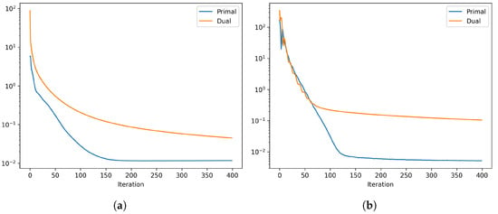
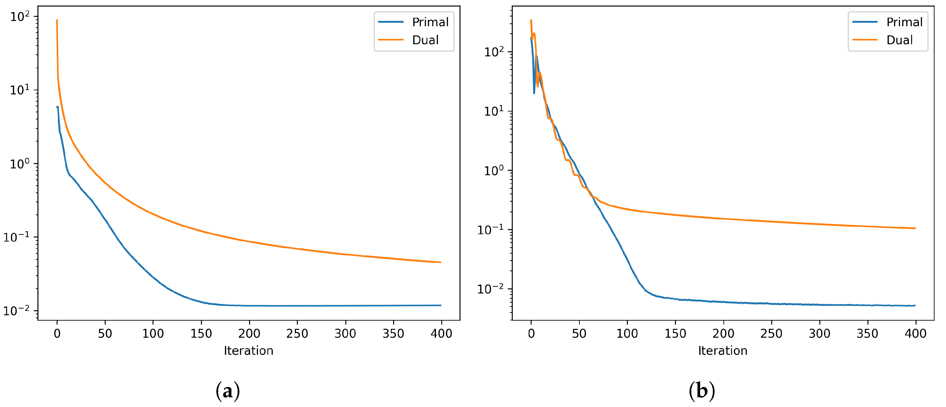
For the Plug-and-Play ADMM implementation, we utilize the SCICO (Scientific Computational Imaging Code) library, which provides a modular framework for defining forward operators, ADMM solvers, and learned denoisers [85]. Two regularization terms are incorporated: a pretrained DnCNN denoiser (17M), a 17-layer network trained on natural images with medium Gaussian noise, for learned spatial prior; and a simplex projection to enforce the ANC and ASC constraints. Since the pretrained DnCNN is a two-dimensional denoising network, the hyperspectral data are processed band-by-band in the denoising step rather than as a full three-dimensional spectral tensor. Therefore, the DnCNN mainly provides a learned spatial prior, while the spectral mixing information is handled through the forward model and abundance constraints. The ADMM penalty parameters are denoted as , corresponding to the DnCNN denoising prior and simplex projection, respectively. The denoising penalty was selected empirically for each dataset and blur scenario within the range to , while the simplex penalty was fixed at to strictly enforce the abundance constraints. These values were selected empirically by testing several candidate settings and choosing the ones that provided stable residual behavior and the best overall quantitative performance. For all experiments, the proposed PnP-JDU method was executed for 400 iterations, as the ADMM primal and dual residual curves (Figure 1) plateaued at this stage. Figure 1a,b show the evolution of the primal and dual residuals over ADMM iterations for the two datasets used in this study: Indian Pines and Pavia University. The primal and dual residual curves decrease steadily and reach stable plateaus, indicating that the Plug-and-Play ADMM iterations stabilize under the chosen penalty parameters.
Figure 1.
Evolution of Plug-and-Play ADMM shown by primal and dual residuals for (a) Indian Pines and (b) Pavia University.
4. Experimental Setup
We conducted a comprehensive performance evaluation of the proposed framework on widely used hyperspectral datasets including Indian Pines [86] and Pavia University [87], which we degrade using Gaussian kernels of varying bandwidths, motion blur, and square blur to create blurred data for our study. The results are assessed and compared with those of existing methods quantitatively using standard image-quality and spectral-fidelity metrics: Root-Mean-Square Error (RMSE), Peak Signal-to-Noise Ratio (PSNR), Spectral Angle Distance (SAD), and Erreur Relative Globale Adimensionnelle de Synthèse (ERGAS) [88]. All experiments were performed on a workstation equipped with an Intel Core i9-14900K CPU, 62 GiB system memory, and an NVIDIA GeForce RTX 4090 GPU with 24 GiB memory. The same hardware configuration was used for all runtime measurements.
4.1. Degradation Models
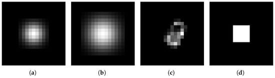
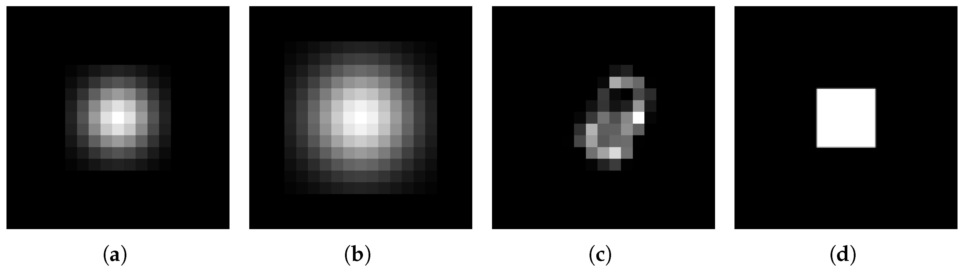
To simulate degradation, we follow the settings used in prior works [77,89], where each dataset is convolved with a set of representative blur kernels and then corrupted by additive zero-mean Gaussian noise. The considered degradations include: (i) a Gaussian kernel with bandwidth 2 and a zero-mean Gaussian noise with ; (ii) a Gaussian kernel with bandwidth 3 and a zero-mean Gaussian noise with ; (iii) a Gaussian kernel with bandwidth 2 and a zero-mean Gaussian noise with ; (iv) a motion blur kernel of size with a zero-mean Gaussian noise ; and (v) a square blur kernel with side length 5 and a zero-mean Gaussian noise (see Figure 2).
Figure 2.
Blurring kernels used in the experiments: (a) Gaussian kernel, (b) Gaussian kernel, (c) Motion kernel, and (d) Square kernel, respectively.
The signal-to-noise ratio (SNR, in dB) for additive zero-mean Gaussian noise decreases as the noise level increases. For a noise standard deviation of , the SNR is 25 for the Indian Pines dataset and 24 for the Pavia University dataset. When the noise standard deviation is increased to , the SNR drops to 16 for the Indian Pines and 15 for the Pavia University.
4.2. Datasets
We evaluated the proposed framework on a set of widely used hyperspectral datasets including the Indian Pines and Pavia University datasets that capture different spatial, spectral, and application characteristics.
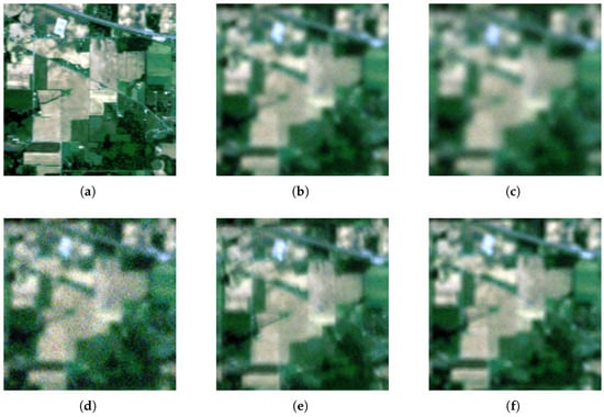
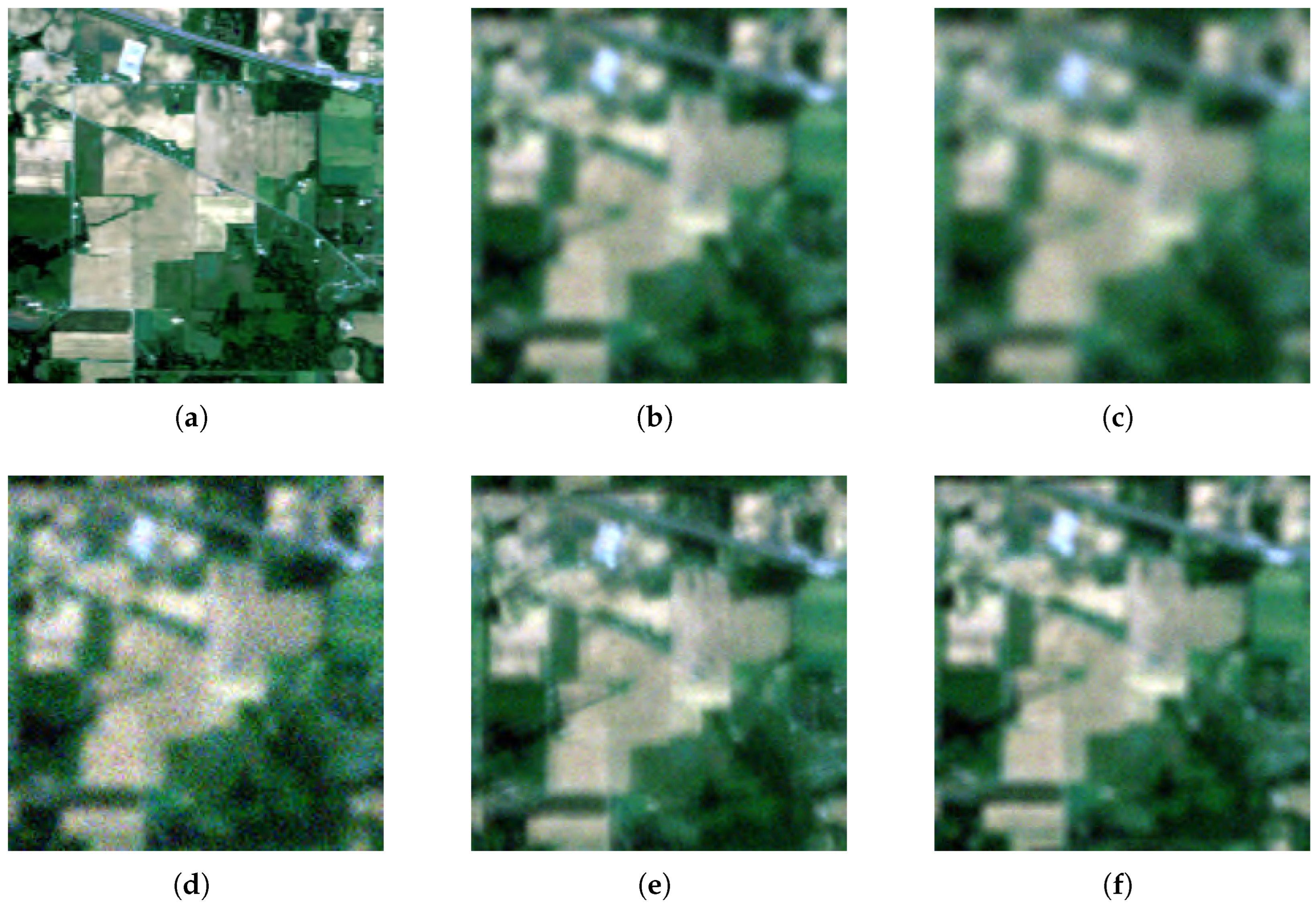
The Indian Pines scene [86], collected by the AVIRIS sensor over northwestern Indiana, consists of pixels with 224 spectral bands spanning 0.4–2.5 m. Following the procedure in [90], we removed the water absorption bands (104–108, 150–163, and 220) to improve data quality. These spectral regions are known to be unreliable due to strong atmospheric water vapor absorption, which attenuates most of the incoming light and results in very low signal-to-noise ratio (SNR) and corrupted reflectance values. The scene is primarily agricultural (two-thirds cropland, one-third forest and perennial vegetation), with additional man-made structures such as roads, highways, and housing. Ground truth covers 16 land-cover classes, though some are not mutually exclusive. An RGB visualization of the Indian Pines dataset is shown in Figure 3, which highlights the original scene, its degraded versions generated using Gaussian, motion and square convolutions, and a further degraded version with additive zero-mean Gaussian noise.
Figure 3.
RGB visualization of the Indian Pines hyperspectral dataset constructed from the closest bands to 650 nm (R), 550 nm (G), and 450 nm (B). (a) Ground truth hyperspectral image; (b) Convolved hyperspectral image with a Gaussian kernel with bandwidth 2 and corrupted by noise with (SNR = 25 ); (c) Convolved hyperspectral image with a Gaussian kernel with bandwidth 3 and corrupted by noise with (SNR = 25 ); (d) Convolved hyperspectral image with a Gaussian kernel with bandwidth 2 and corrupted by noise with (SNR = 16 ); (e) Convolved hyperspectral image with a motion kernel and corrupted by noise with (SNR = 25 ); (f) Convolved hyperspectral image with a square kernel and corrupted by noise with (SNR = 25 ).
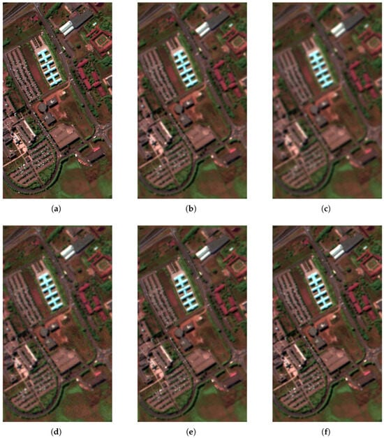
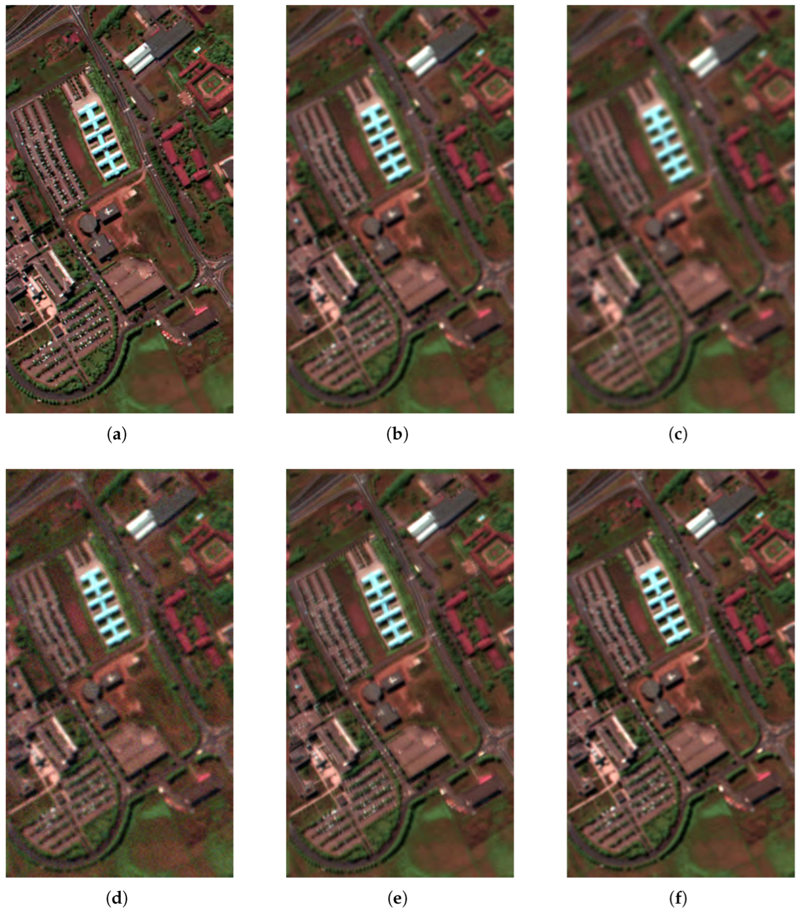
The Pavia University scene [87], acquired by the ROSIS sensor during an airborne campaign over northern Italy, has pixels and 103 spectral bands spanning – m, where each pixel represents a square ground area of 1.3 m × 1.3 m. A portion of the samples corresponds to background with no information, which appears as black strips and is typically discarded before analysis. Ground-truth annotations distinguish nine urban land-cover classes. Figure 4 presents an RGB visualization of the Pavia dataset, illustrating the original scene, its degraded versions obtained through Gaussian, motion and square convolution, and an additional degradation resulting from additive zero-mean Gaussian noise.
Figure 4.
RGB visualization of Pavia University hyperspectral dataset constructed from the closest bands to 650 nm (R), 550 nm (G), and 450 nm (B). (a) Ground truth hyperspectral image; (b) Convolved hyperspectral image with a Gaussian kernel with bandwidth 2 and corrupted by noise with (SNR = 24 ); (c) Convolved hyperspectral image with a Gaussian kernel with bandwidth 3 and corrupted by noise with (SNR = 24 ); (d) Convolved hyperspectral image with a Gaussian kernel with bandwidth 2 and corrupted by noise with (SNR = 15 ); (e) Convolved hyperspectral image with a motion kernel and corrupted by noise with (SNR = 24 ); (f) Convolved hyperspectral image with a square kernel and corrupted by noise with (SNR = 24 ).
4.3. Quantitative Metrics and Baselines
To quantitatively evaluate the performance of the proposed method and compare it to other deconvolution and unmixing methods, several well-established metrics are employed. These metrics assess the accuracy of the reconstructed hyperspectral image and the abundance maps with respect to the ground truth. The following metrics are used:
4.3.1. Hyperspectral Reconstruction Metrics
These metrics evaluate how well the reconstructed hyperspectral dataset (), obtained from the endmember matrix and estimated abundance maps (), match the ground-truth data () which follows the mixing model , reflecting the accuracy of spectral information recovery. All the evaluation metrics defined below are computed between the ground-truth hyperspectral image reconstructed from the ground-truth abundance maps and known endmembers, and the reconstructed hyperspectral image obtained from the estimated abundance maps and the same known endmembers.
- Root-Mean-Square Error (RMSE): RMSE quantifies the average pixel-wise error between the reconstructed and ground truth images. A lower RMSE indicates a more accurate reconstruction:where denotes the spatial height and width of the image, and L denotes the number of spectral bands.
- Peak Signal-to-Noise Ratio (PSNR): PSNR measures the ratio between the maximum possible signal value and the distortion (error) introduced during reconstruction. A higher PSNR indicates better reconstruction:
- Erreur Relative Globale Adimensionnelle de Synthèse (ERGAS): ERGAS measures the global relative error of the reconstructed image and is commonly used in remote sensing. Lower ERGAS values indicate better performance:
- Spectral Angle Distance (SAD): This measures the distortion between the original spectrum and the reconstructed one and lower values indicate better spectral fidelity:
- Structural Similarity Index Measure (SSIM): SSIM evaluates the structural similarity between the reconstructed hyperspectral image and the ground-truth image. Unlike RMSE and PSNR, which mainly quantify pixel-wise reconstruction error, SSIM measures the preservation of spatial structures, contrast, and luminance information. Following the band-wise evaluation commonly used for hyperspectral image deconvolution, SSIM is computed for each spectral band and then averaged over all bands:where and denote the reconstructed and ground-truth images at spectral band ℓ, respectively. The terms and are the mean intensities, and are the standard deviations, and is the covariance between the reconstructed and ground-truth images at band ℓ. The constants and are small positive values used to stabilize the division. A higher SSIM value indicates better preservation of spatial structure in the reconstructed hyperspectral image.
4.3.2. Abundance Map Metric
- Root Mean Square Error for abundances (aRMSE): It measures the deviation between the estimated abundances and the ground-truth abundances over pixels and P endmembers:A smaller aRMSE indicates more accurate abundance estimation.
5. Experimental Results
5.1. Performance Evaluation on Indian Pines Dataset
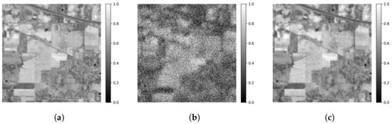
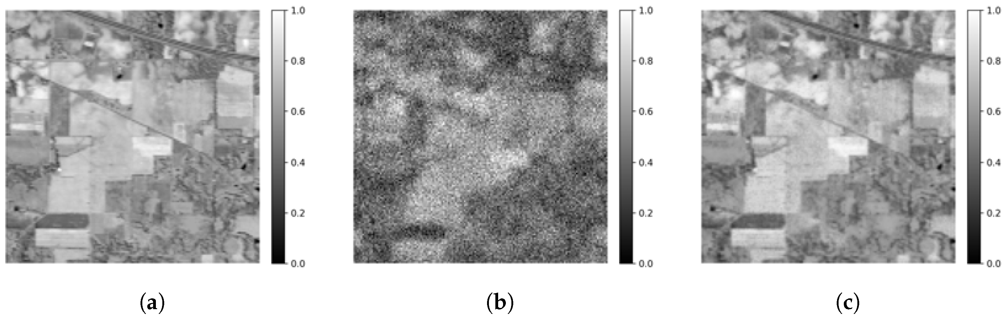
To validate the feasibility of the proposed joint deblurring–unmixing PnP-JDU framework, we conducted experiments on the Indian Pines dataset under controlled Gaussian, motion, and square blur degradations (Figure 3). Figure 5 shows the Indian Pines band 100 under motion blur degradation. The motion-blurred and noisy observation in (Figure 5b) severely obscures spatial boundaries and texture present in the ground truth shown in (Figure 5a). The PnP-JDU reconstructed result in (Figure 5c) recovers sharp edges and homogeneous regions, highlighting the robustness of the proposed joint deconvolution and unmixing approach to complex, non-isotropic blur.
Figure 5.
Comparison of Indian Pines band 100 (wavelength m) across the Ground truth, Motion kernel and corrupted by noise with , and PnP-JDU reconstructed hyperspectral image.
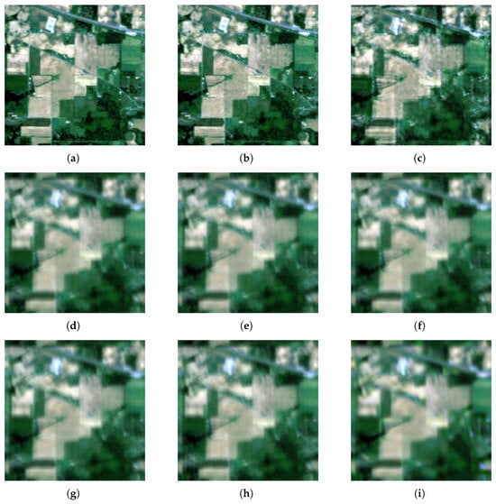
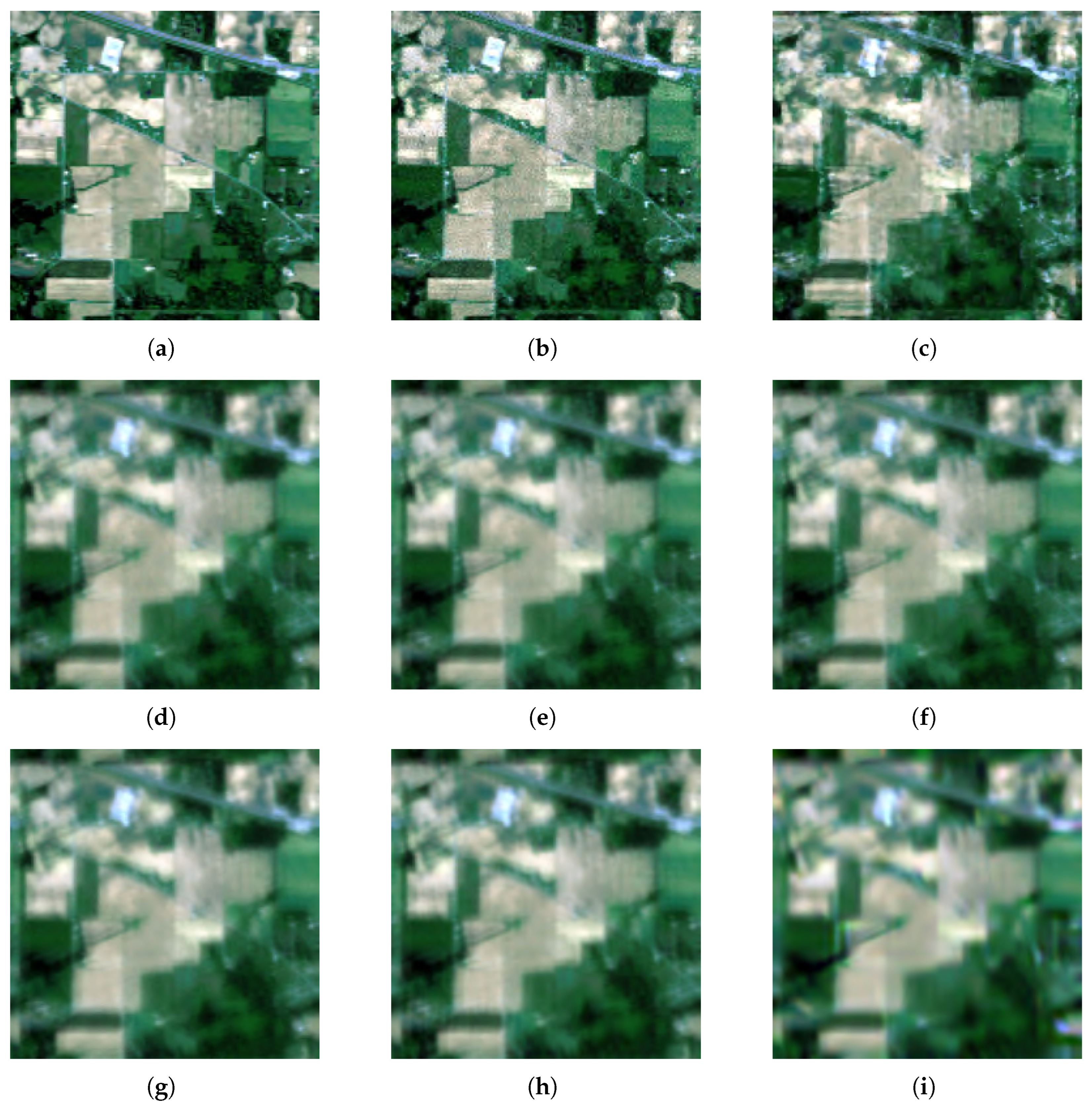
The performance of the proposed PnP-JDU model was compared against classical unmixing approaches, including Unconstrained Least Squares (UCLS), Fully Constrained Least Squares (FCLS), Nonnegative Least Squares (NCLS), standard Plug-and-Play unmixing approaches, including Pro-A/H-NLM, Pro-A/H-BM3D [63,64] without explicit deblurring and DSUnADM-TV [22]. The reconstructed hyperspectral images obtained from each method are shown in Figure 6.
Figure 6.
Indian Pines hyperspectral image reconstructions under motion blur and additive noise with using different unmixing methods. (a) Ground truth, (b) PnP-JDU, (c) DSUnADM-TV, (d) UCLS, (e) FCLS, (f) NCLS, (g) PnP-U, (h) Pro-H-NLM, and (i) Pro-H-BM3D.
The visual results clearly demonstrate that the proposed PnP-JDU algorithm achieves a notably sharper reconstruction compared with all the baseline methods. The UCLS, FCLS, NCLS, PnP-U, Pro-H-NLM, and Pro-H-BM3D reconstructions exhibit spatial smoothing, loss of fine-scale texture, and residual blurring around object boundaries. While DSUnADM-TV improves reconstruction quality over these baselines by reducing blur and preserving structural information, certain fine details remain less sharp than those in the proposed PnP-JDU result. In contrast, the PnP-JDU output recovers distinct field structures and edge details that closely resemble the ground truth. This improvement highlights the importance of jointly handling blur and spectral mixing within a unified optimization framework rather than treating them as separate processes, as well as the benefit of the PnP prior over the TV regularizer.
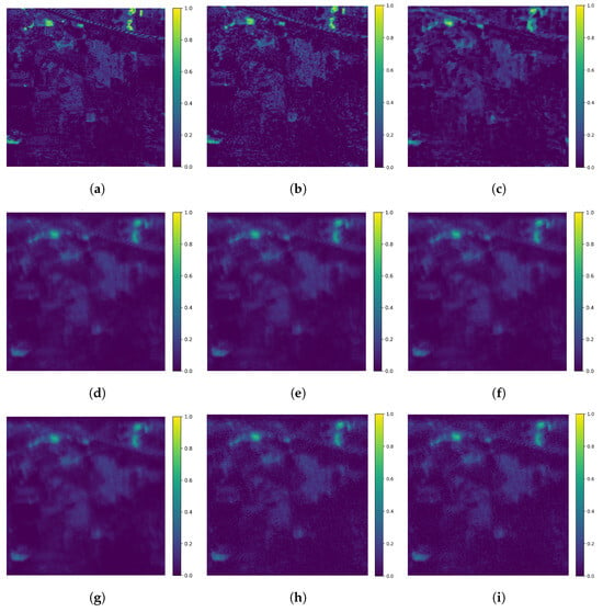
To further assess the accuracy of abundance estimation, endmember 4 was selected because its abundance map contains specific, concentrated high-abundance regions with clear transitions from the surrounding low-abundance background. The estimated abundance maps shown in Figure 7 reveal that PnP-JDU (Figure 7b) preserves spatial consistency and delineates class boundaries more accurately than the other methods. The abundance maps derived from UCLS, NCLS, and FCLS show significant spatial leakage between adjacent regions. The PnP-U, Pro-A-NLM, and Pro-A-BM3D methods, although leveraging learned priors, lack explicit modeling of the degradation process and, thus, retain residual blurring. DSUnADM-TV outperforms the baseline methods in terms of blur reduction and structural preservation; nevertheless, the proposed PnP-JDU approach yields superior sharpness in fine-scale details. In contrast, PnP-JDU effectively suppresses spatial artifacts and recovers smooth yet sharp abundance transitions consistent with the ground truth distribution. These visual observations confirm that embedding the deconvolution operator within the PnP-ADMM optimization allows the algorithm to exploit both data fidelity to the blurred observation and spatial correlations captured by the denoiser, resulting in more realistic and interpretable abundance maps.
Figure 7.
Abundance maps for endmember 4 generated by different unmixing methods from the Indian Pines dataset under motion blur and additive noise with . (a) Ground truth, (b) PnP-JDU, (c) DSUnADM-TV, (d) UCLS, (e) FCLS, (f) NCLS, (g) PnP-U, (h) Pro-A-NLM, and (i) Pro-A-BM3D.
Quantitative comparisons under different blur conditions are summarized in Table 1, where the methods are evaluated using the metrics defined in Section 4.3. Across all degradation types, the proposed PnP-JDU consistently achieves the lowest error values and the highest PSNR. It outperforms the classical least-squares methods and standard PnP frameworks by a substantial margin, while also providing consistent improvements over DSUnADM-TV. Specifically, under the Gaussian (9, 9, 2) blur condition with additive Gaussian noise at an SNR of 25 , PnP-JDU attains an aRMSE of and a PSNR of , compared with aRMSE and PSNR for FCLS, UCLS, NCLS, and PnP frameworks. DSUnADM-TV performs closer to PnP-JDU than the non-joint baselines, indicating the benefit of joint deblurring and unmixing. The same trend is observed in the SSIM values. PnP-JDU achieves lower error values and higher reconstruction quality, with runtime higher than the simple least-squares and iterative DSUnADM-TV methods, but lower than the NLM- and BM3D-based baselines.
Table 1.
Comparison results from different methods on the Indian Pines dataset under simulated degradations. The hyperspectral image is blurred according to predefined scenarios and contaminated with additive zero-mean Gaussian noise. Results are summarized over 20 independent noise realizations. The best results are highlighted in bold. ↑ indicates a higher value is better; ↓ indicates a lower value is better.
As expected, this superiority persists under stronger blur and noise scenarios, including Gaussian (13, 13, 3) and Gaussian (9, 9, 2) at SNR . In these cases, PnP-JDU reduces the reconstruction RMSE by approximately – times relative to the classical unmixing methods and other PnP-based frameworks. Compared with DSUnADM-TV, the improvement is smaller but still consistent, indicating that the proposed joint PnP framework provides the best overall reconstruction accuracy. Similar trends are observed for structured degradations. Under motion blur, PnP-JDU achieves a PSNR of , while the classical unmixing methods and PnP frameworks remain around 25– and DSUnADM-TV reaches . In addition, the SSIM values confirm this trend. The corresponding ERGAS scores further support these findings, with PnP-JDU consistently producing the smallest global relative synthesis error across the tested blur kernels.
5.1.1. Ablation Study on the Indian Pines Dataset
To quantify the contribution of each prior/constraint in the proposed PnP-JDU framework, an ablation study was conducted on the Indian Pines dataset under the Gaussian (13, 13, 3) degradation with additive Gaussian noise at SNR . The experiment was repeated over 10 independent noise realizations, and the results are reported as mean ± standard deviation in Table 2. The DnCNN module acts as a learned plug-and-play denoising prior, while the simplex projection enforces abundance nonnegativity and sum-to-one constraints.
Table 2.
Ablation study results for the Indian Pines dataset under the Gaussian (13, 13, 3) blur with SNR = 25 . Values are reported as mean ± standard deviation over independent noise realizations. ↑ indicates a higher value is better; ↓ indicates a lower value is better.
The ablation results show that the simplex projection improves both abundance estimation and reconstructed image quality in terms of the ERGAS metric. The DnCNN is also shown to improve abundance estimation and the reconstruction quality particularly in terms of the PSNR. All the metrics improve when both the Simplex and DnCNN are used. These results indicate that enforcing the physical abundance constraints and regularization through the DnCNN prior are both essential for stable and accurate joint deconvolution and unmixing.
5.1.2. Computational Runtime Analysis for the Indian Pines Dataset
For the Indian Pines dataset, the runtime per iteration was compared only among the iterative methods. PnP-U required 0.04 s/iteration, while the proposed PnP-JDU required 0.10 s/iteration. DSUnADM-TV required 0.11 s/iteration. Therefore, PnP-JDU is more computationally expensive than PnP-U but slightly faster per iteration than DSUnADM-TV for Indian Pines. In contrast, the NLM- and BM3D-based plug-and-play methods were much slower, requiring 16.89 and 30.28 s/iteration, respectively. These results show that PnP-JDU provides improved reconstruction and abundance-estimation performance while maintaining a practical computational cost.
5.2. Performance Evaluation on Pavia University Dataset
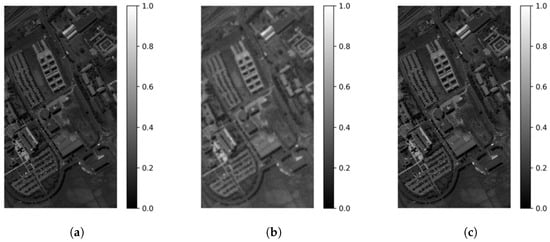
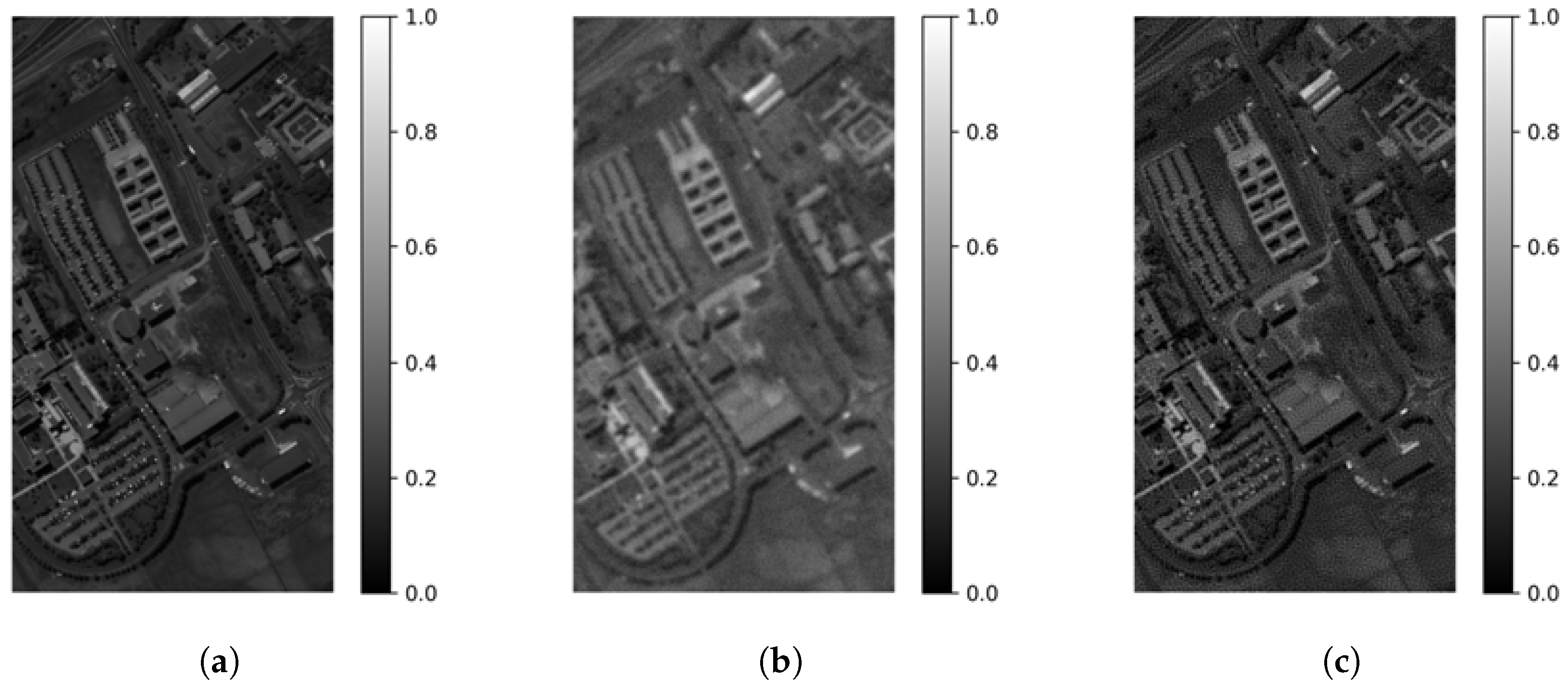
To further evaluate the robustness and generalization of the proposed PnP-JDU framework, experiments were conducted on the Pavia University dataset, which represents an urban environment. Similar to the previous setup, the hyperspectral image was degraded using Gaussian, motion, and square blur kernels, followed by the addition of zero-mean Gaussian noise (Figure 4). Figure 8 illustrates the effect of joint deconvolution and unmixing on Pavia University Band 50. The Gaussian-blurred and noisy observation in Figure 8b exhibits significant loss of spatial detail and contrast compared to the ground truth in Figure 8a. The reconstructed image in Figure 8c demonstrates effective recovery of fine spatial structures and intensity levels, indicating that the proposed joint framework successfully mitigates blur and noise while preserving spectral fidelity.
Figure 8.
Comparison of Pavia University Band 50 (wavelength m) across the ground truth, Gaussian blur (bandwidth = 3) and corrupted by noise with , and PnP-JDU reconstructed hyperspectral image.
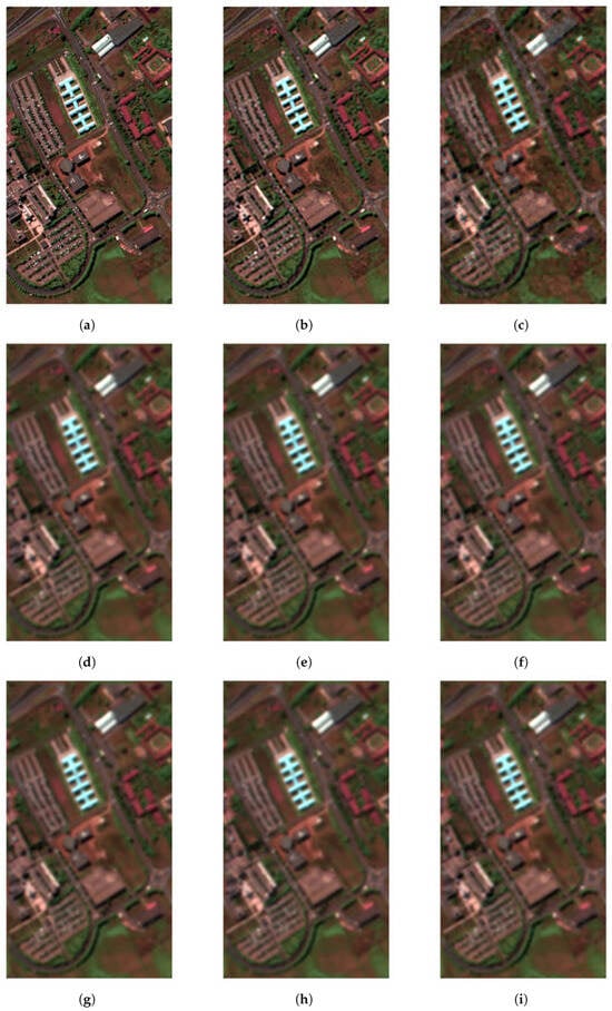
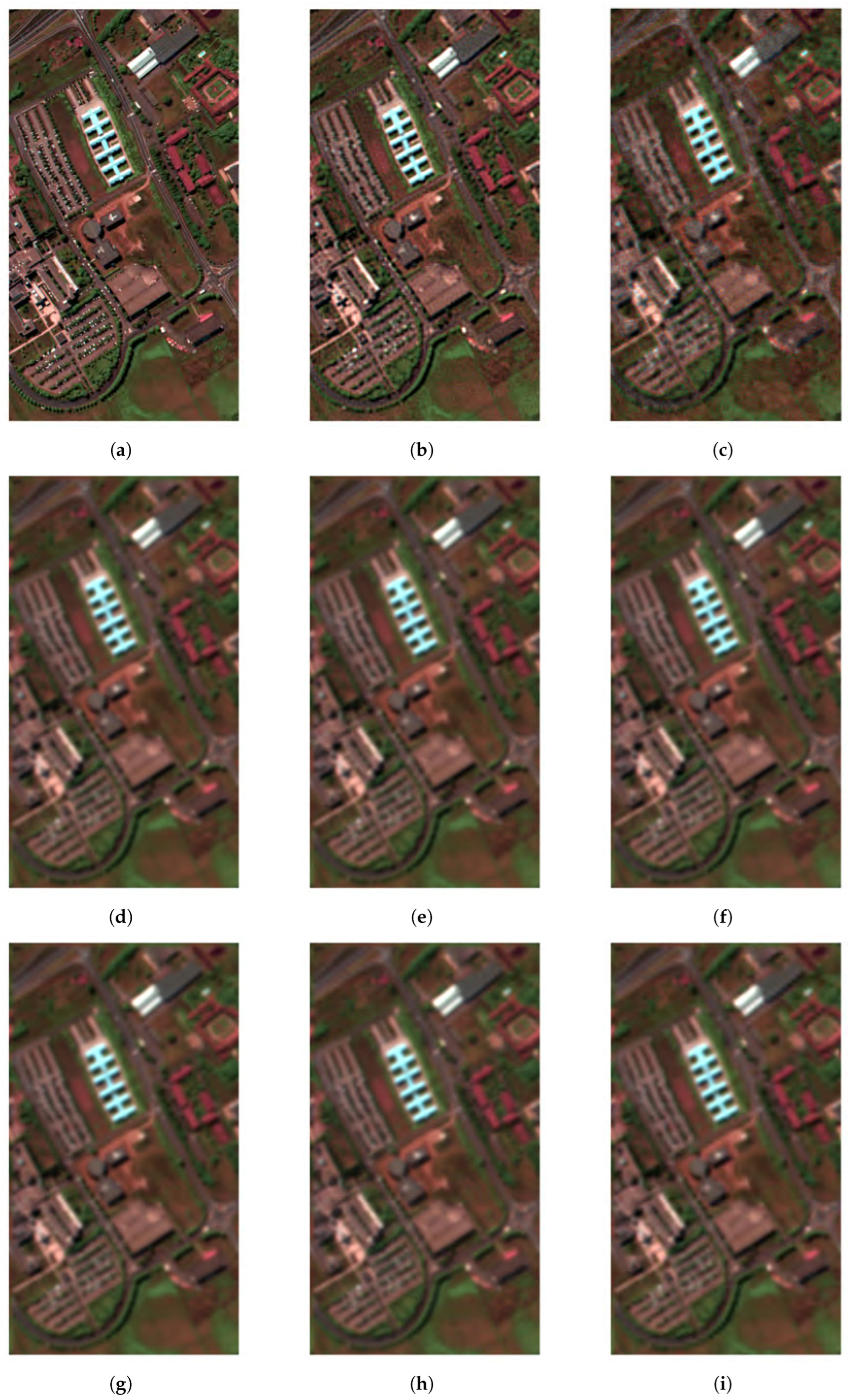
The results of PnP-JDU were compared with those of classical unmixing methods—UCLS, FCLS, and NCLS—the standard Plug-and-Play unmixing approaches without explicit deblurring (PnP-U, Pro-A/H-NLM, and Pro-A/H-BM3D) and the TV/sparsity-based joint deblurring–unmixing baseline DSUnADM-TV. Figure 9 shows the reconstructed hyperspectral images obtained by all investigated methods. It can be observed that the classical methods produce oversmoothed reconstructions with loss of fine spatial details, while the PnP approaches reduce noise but retain residual blur. DSUnADM-TV improves the reconstruction compared with the classical and PnP baselines; however, some spatial smoothing and loss of fine structural details remain. In contrast, the proposed PnP-JDU framework yields the sharpest reconstruction, with clear structural boundaries and enhanced contrast. This improvement is particularly visible in urban regions, such as building edges and road intersections, where blur removal is critical for accurate material discrimination.
Figure 9.
Reconstructed Pavia University hyperspectral images obtained using different unmixing methods under degradation by a Gaussian blur kernel (bandwidth = 3) and additive zero-mean Gaussian noise with standard deviation . (a) Ground truth, (b) PnP-JDU, (c) DSUnADM-TV, (d) UCLS, (e) FCLS, (f) NCLS, (g) PnP-U, (h) Pro-H-NLM, and (i) Pro-H-BM3D.
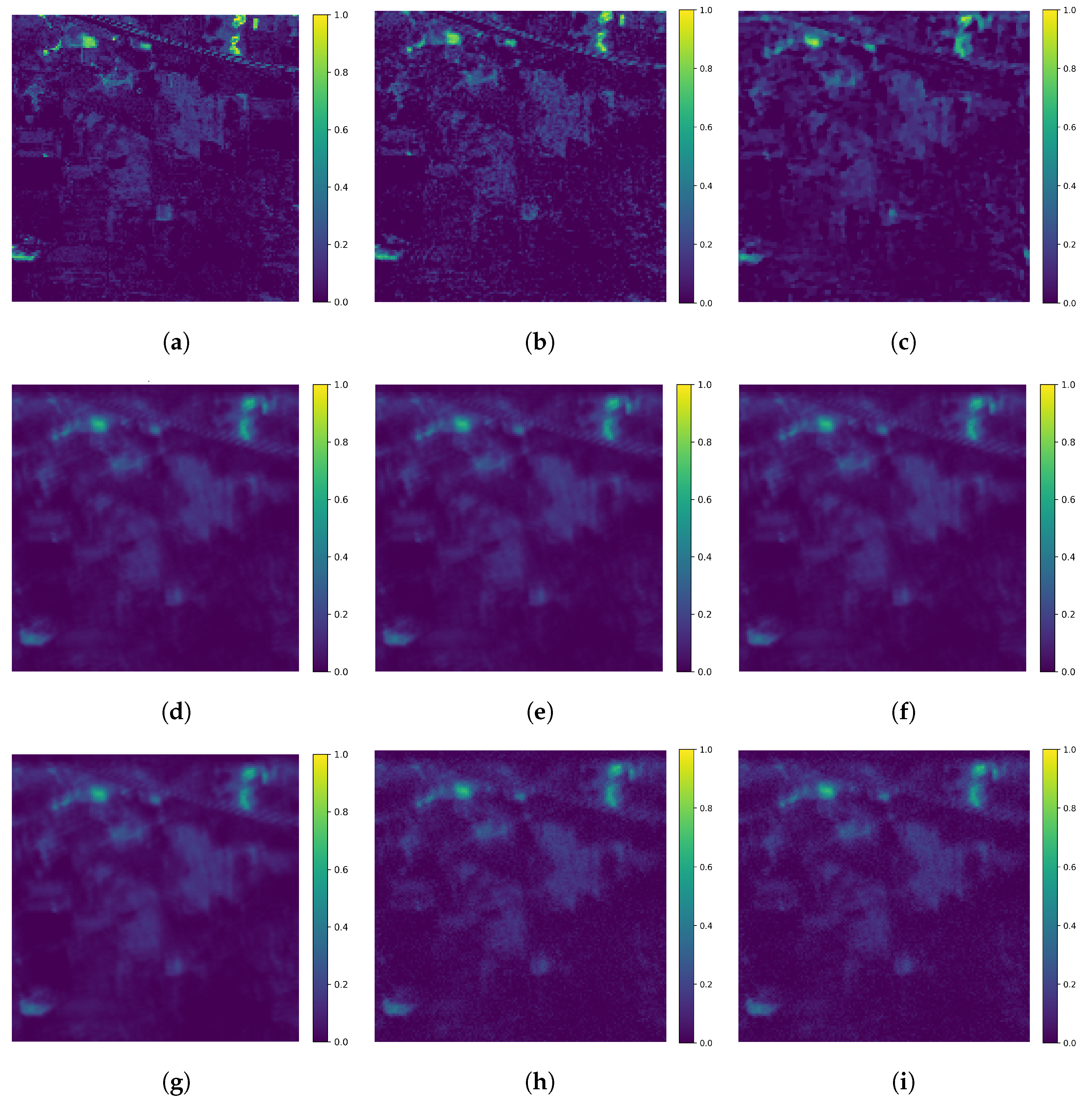
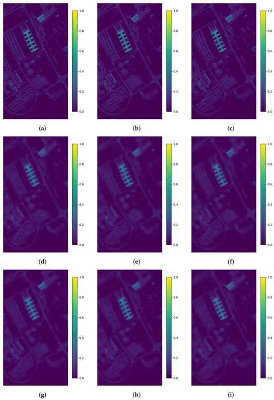
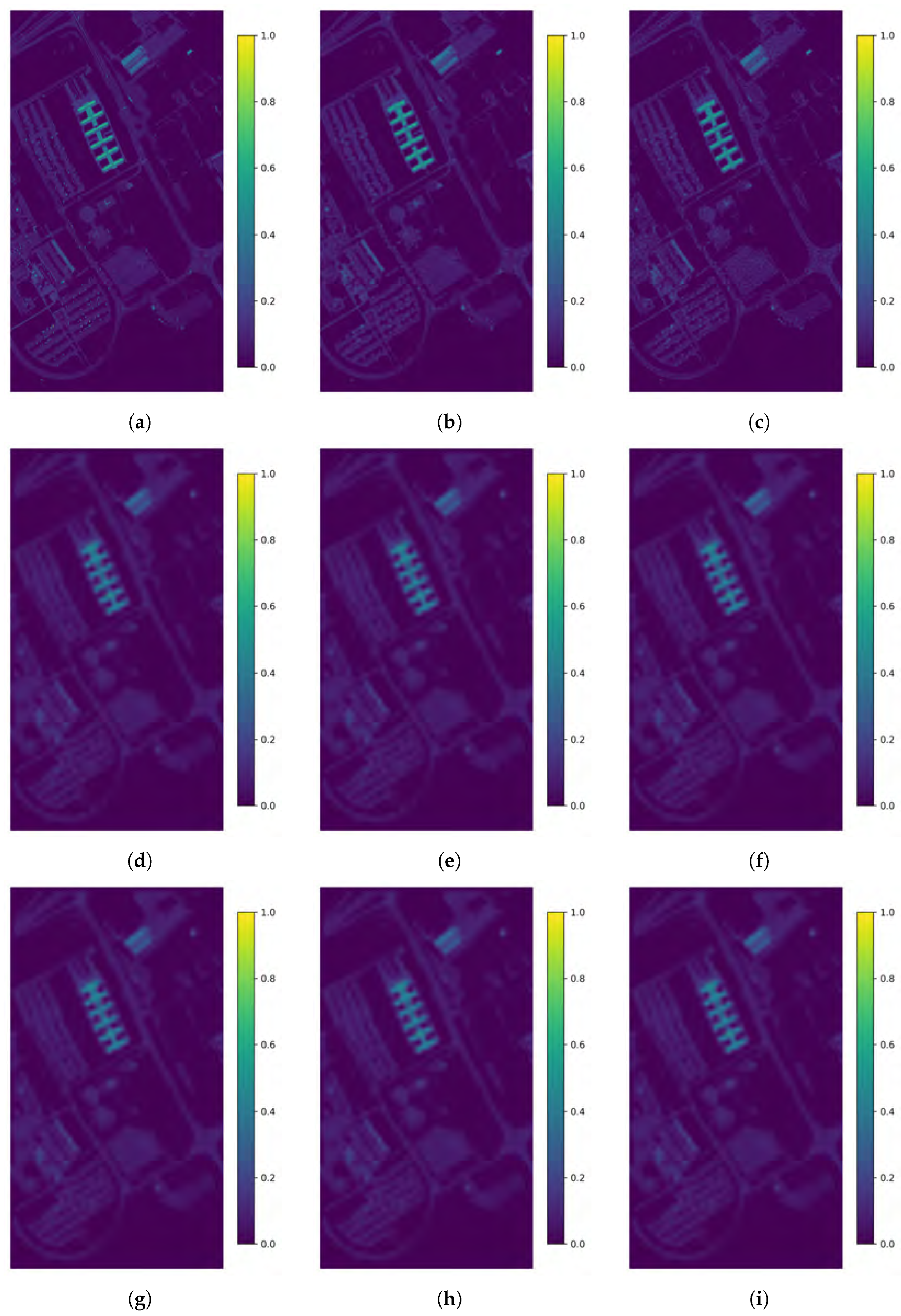
To analyze the abundance estimation performance, Figure 10 presents the abundance maps corresponding to endmember 4, chosen because it highlights the sharp edges of a building. The PnP-JDU abundance map (Figure 10b) exhibits sharper delineation of material boundaries and improved structural information of fine details compared to all baselines. In contrast, abundance maps from FCLS, UCLS, and NCLS display significant spatial leakage between adjacent regions, while the PnP-U, Pro-A-NLM, and Pro-A-BM3D results fail to restore small-scale variations lost due to blur. Additionally, DSUnADM-TV provides improvement by reducing blur, and qualitatively the result is similar to the one from PnP-JDU.
Figure 10.
Abundance maps for endmember 4 generated by different unmixing methods from the Pavia University dataset under degradation by a Gaussian blur kernel (bandwidth = 3) and additive zero-mean Gaussian noise with standard deviation . (a) Ground truth, (b) PnP-JDU, (c) DSUnADM-TV, (d) UCLS, (e) FCLS, (f) NCLS, (g) PnP-U, (h) Pro-A-NLM, and (i) Pro-A-BM3D.
Quantitative results summarized in Table 3 further substantiate these visual observations. Across all degradation scenarios, PnP-JDU consistently achieves the lowest aRMSE and RMSE values, the highest PSNR and SSIM, and the smallest ERGAS, indicating superior reconstruction fidelity and abundance accuracy. For example, under the Gaussian (9, 9, 2) blur condition with additive Gaussian noise at an SNR of , PnP-JDU attains an aRMSE of almost and a PSNR of , substantially outperforming all other methods, such as FCLS, PnP frameworks, and provides improvement over the DSUnADM-TV metrics. Similar improvements are observed for stronger blur scenarios such as Gaussian (13, 13, 3), where PnP-JDU reduces ERGAS from approximately 46 for non-joint baselines to . Compared with the joint DSUnADM-TV baseline, which achieves an ERGAS of 26.23, the proposed method still provides a further reduction, indicating improved global reconstruction fidelity under stronger blur. Even under motion and square blur, PnP-JDU maintains PSNR values above and ERGAS below 12 and SSIM above , demonstrating stable performance across diverse imaging conditions, with increased runtime compared with the faster least-squares and iterative DSUnADM-TV methods, but still below the BM3D-based baseline. These findings confirm that explicitly incorporating the deconvolution operator within the PnP-ADMM optimization enables PnP-JDU to better exploit spatial–spectral correlations while preserving abundance smoothness and structural integrity.
Table 3.
Comparison results from different methods on the Pavia University dataset under simulated degradations. The hyperspectral image is blurred according to predefined scenarios and contaminated with additive zero-mean Gaussian noise. Results are summarized over 20 independent noise realizations. The best results are highlighted in bold. ↑ indicates a higher value is better; ↓ indicates a lower value is better.
5.2.1. Ablation Study on the Pavia University Dataset
To quantify the contribution of each prior/constraint in the proposed PnP-JDU framework, an ablation study was conducted on the Pavia University dataset under motion blur with additive Gaussian noise at SNR . The experiment was repeated over 10 independent noise realizations, and the results are reported as mean ± standard deviation in Table 4. As mentioned earlier, the DnCNN module acts as a learned plug-and-play denoising prior, while the simplex projection enforces abundance nonnegativity and sum-to-one constraints.
Table 4.
Ablation study results for the Pavia University datase under the motion blur scenario with SNR = 24 . Values are reported as mean ± standard deviation over independent noise realizations. ↑ indicates a higher value is better; ↓ indicates a lower value is better.
The ablation results show that both the simplex projection and DnCNN improve abundance estimation and reconstructed image quality when added to the data fidelity term, with the simplex projection having a greater impact. These results confirm that enforcing physically valid abundance constraints and regularization with a good prior are essential for stable and accurate joint deconvolution and unmixing under motion-blur degradation.
5.2.2. Computational Runtime Analysis for the Pavia University Dataset
For the larger Pavia University dataset, the runtime per iteration increased for all iterative methods due to the larger spectral and spatial size of the data. PnP-U required 0.15 s/iteration, while DSUnADM-TV required 0.41 s/iteration based on its reported iteration count. The proposed PnP-JDU required 0.66 s/iteration. Although PnP-JDU is computationally more demanding than PnP-U and DSUnADM-TV on Pavia University, it remains substantially faster than the NLM- and BM3D-based plug-and-play methods, which required 10.10 and 78.88 s/iteration, respectively. Overall, the runtime results indicate that PnP-JDU introduces additional computational cost, but this cost remains reasonable considering its improved restoration and unmixing accuracy.
6. Discussion
The experimental results demonstrate that explicitly coupling deconvolution and spectral unmixing within a single optimization framework improves both hyperspectral image reconstruction and abundance estimation. Across the Indian Pines and Pavia University datasets, the proposed PnP-JDU method consistently achieved lower reconstruction and abundance errors, higher PSNR and SSIM values, and lower SAD and ERGAS values than the classical unmixing baselines and the standalone PnP unmixing methods. These results indicate that modeling blur directly within the unmixing problem is important, since methods that do not explicitly account for the degradation process retain residual blur and lose fine spatial details.
The comparison with DSUnADM-TV further shows the benefit of replacing hand-crafted regularization with a learned plug-and-play prior. Although DSUnADM-TV also performs joint deblurring and unmixing and improves over the non-joint baselines, PnP-JDU provides sharper reconstructions and more accurate abundance maps in most tested degradation scenarios. This suggests that the learned DnCNN prior can better capture spatial structure than the TV-based regularizer while the simplex projection maintains physically meaningful abundance estimates.
The ablation studies confirm that both the simplex projection and the DnCNN prior contribute to the performance of the proposed framework. The simplex projection enforces the abundance nonnegativity and sum-to-one constraints, which improves the physical validity and stability of the abundance estimates. The DnCNN prior improves reconstruction quality by introducing learned spatial regularization within the ADMM framework. The best performance is obtained when both components are used together, showing that the combination of physical constraints and learned prior information is essential for accurate joint deconvolution and unmixing.
The runtime analysis shows that PnP-JDU introduces additional computational cost compared with simpler pixel-wise methods and standalone PnP unmixing. This increase is expected because PnP-JDU solves a joint inverse problem and requires repeated data-fidelity, denoising, simplex-projection, and dual-update steps. However, the method remains substantially faster than the NLM- and BM3D-based plug-and-play baselines and provides a favorable trade-off between computational cost and reconstruction accuracy. Therefore, the additional runtime is justified by the improved abundance-estimation and deblurring performance.
7. Conclusions
In this work, we presented a novel joint hyperspectral image deconvolution and unmixing framework based on the Plug-and-Play paradigm (PnP-JDU). By integrating a learned DnCNN denoiser as an implicit prior within the ADMM physics-informed optimization scheme, the proposed method simultaneously addresses spatial blur and spectral mixing—two key sources of degradation in hyperspectral imaging. The ADMM-based splitting enables separate handling of the data fidelity and prior/constraint terms, effectively combining model-based physical consistency with data-driven spatial regularization. Experiments on the Indian Pines and Pavia University datasets under multiple blur and noise conditions demonstrate that PnP-JDU achieves superior performance compared to classical unmixing and restoration baselines, including FCLS, UCLS, standard PnP unmixing methods that use different denoisers than ours, and the TV/sparsity-based DSUnADM-TV, which is a joint deconvolution and unmixing framework that does not employ PnP priors. These results collectively demonstrate that the integration of spatial deconvolution within the unmixing process and the use of the PnP prior and simplex projection used in our method markedly enhances both spectral fidelity and spatial detail preservation. The PnP-JDU framework consistently produced the lowest reconstruction and abundance errors, the highest PSNR and SSIM, and the lowest SAD scores, while preserving fine spatial details and maintaining physically meaningful abundance maps. Overall, the proposed PnP-JDU framework establishes a solid foundation for physically interpretable, data-driven hyperspectral reconstruction, bridging the gap between traditional model-based optimization and modern learning-based restoration techniques.
Despite its strong performance, the proposed PnP-JDU framework has two main limitations. First, it requires higher computational time than simpler pixel-wise or closed-form unmixing methods because it relies on iterative PnP-ADMM optimization with repeated data-fidelity, denoising, simplex-projection, and regularization updates. However, its computational cost relative to DSUnADM-TV is dataset dependent. In the Indian Pines experiment, PnP-JDU was slightly faster per iteration than DSUnADM-TV, with runtimes of 0.10 and 0.11 s/iteration, respectively. In contrast, PnP-JDU was slower in the Pavia University experiment, requiring 0.66 s/iteration compared with 0.41 s/iteration for DSUnADM-TV. Second, the current formulation does not provide a formal convergence guarantee, since the DnCNN denoiser is used as an implicit prior and is combined with simplex projection. Therefore, the residual plots should be interpreted as evidence of empirical stabilization rather than a theoretical proof of convergence.
While the current study focuses on the linear mixing model and assumes known endmembers, several promising directions remain for future research. In particular, extending the proposed framework to more complex real-world scenarios, such as those encountered in mineralogical analysis, planetary surface characterization, and astronomical hyperspectral observations, where the telescope blur kernel can be characterized and used for the deconvolution, represents an important future direction [91,92]. Additionally, applying the proposed PnP-JDU approach to real-world airborne and satellite datasets, where the blur kernel and noise statistics are unknown, represents an important step toward operational deployment.
Author Contributions
Conceptualization, S.L. and C.P.; Methodology, S.L. and C.P.; Writing—original draft preparation, S.L.; Writing—review & editing, S.L. and C.P.; Supervision and project administration, C.P.; Funding acquisition, C.P. All authors have read and agreed to the published version of the manuscript.
Funding
This research was sponsored by the Army Research Laboratory and was accomplished under Cooperative Agreement Number W911NF-21-2-0294 with Eddie L. Jacobs as PI and C.P. as one of the Co-PIs. The views and conclusions contained in this document are those of the authors and should not be interpreted as representing the official policies, either expressed or implied, of the Army Research Office or the US Government. The US Government is authorized to reproduce and distribute reprints for Government purposes notwithstanding any copyright notation herein. Distribution Statement A. Approved for public release: distribution is unlimited.
Data Availability Statement
Our code repository will be made privately available upon reasonable request to the corresponding author.
Acknowledgments
During the preparation of this manuscript/study, the authors used ChatGPT (GPT-5.5) [93] solely for grammar checking and for improving clarity, cohesion, and tone of the text. The authors have reviewed and edited the output and take full responsibility for the content of this publication.
Conflicts of Interest
The authors declare no conflict of interest.
Abbreviations
The following abbreviations are used in this manuscript:
| HSI | Hyperspectral imaging |
| PnP | Plug-and-Play |
| PnP-U | Plug-and-Play Unmixing |
| PnP-JDU | Plug-and-Play Joint Deconvolution and Unmixing |
| LMM | Linear Mixing Model |
| NMM | Nonlinear Mixing Model |
| UCLS | Unconstrained Least Squares |
| NCLS | Nonnegative Constrained Least Squares |
| FCLS | Fully Constrained Least Squares |
| NMF | Nonnegative Matrix Factorization |
| TV | Total Variation |
| ADMM | Alternating Direction Method of Multipliers |
| NLM | Non-Local Means |
| BM3D | Block-Matching and 3D Filtering |
| Pro-NLM | Proposed method with NLM denoiser |
| Pro-BM3D | Proposed method with BM3D denoiser |
| DSUnADM-TV | Deblurring and Sparse Unmixing via Alternating Direction Method with Total Variation |
| BM4D | Block-Matching and 4D Filtering |
| CNN | Convolutional Neural Networks |
| DnCNN | Denoising Convolutional Neural Network |
| MSE | Mean Squared Error |
| ANC | Abundance Nonnegativity Constraint |
| ASC | Abundance Sum-to-One Constraint |
| RMSE | Root-Mean-Square Error |
| PSNR | Peak Signal-to-Noise Ratio |
| ERGAS | Erreur Relative Globale Adimensionnelle de Synthèse |
| SAD | Spectral Angle Distance |
| SCICO | Scientific Computational Imaging Code |
References
- Wang, L.; Zhao, C. Hyperspectral Image Processing; Springer: Berlin/Heidelberg, Germany, 2016. [Google Scholar]
- Keshava, N.; Mustard, J. Spectral Unmixing. IEEE Signal Process. Mag. 2002, 19, 44–57. [Google Scholar] [CrossRef] [Scilit]
- Wei, J.; Wang, X. An Overview on Linear Unmixing of Hyperspectral Data. Math. Probl. Eng. 2020, 2020, 3735403. [Google Scholar] [CrossRef] [Scilit]
- Heylen, R.; Parente, M.; Gader, P. A Review of Nonlinear Hyperspectral Unmixing Methods. IEEE J. Sel. Top. Appl. Earth Obs. Remote Sens. 2014, 7, 1844–1868. [Google Scholar] [CrossRef] [Scilit]
- Dobigeon, N.; Tourneret, J.Y.; Richard, C.; Bermudez, J.C.M.; McLaughlin, S.; Hero, A.O. Nonlinear Unmixing of Hyperspectral Images: Models and Algorithms. IEEE Signal Process. Mag. 2013, 31, 82–94. [Google Scholar] [CrossRef] [Scilit]
- Plaza, A.; Benediktsson, J.A.; Boardman, J.W.; Brazile, J.; Bruzzone, L.; Camps-Valls, G.; Chanussot, J.; Fauvel, M.; Gamba, P.; Gualtieri, A.; et al. Recent advances in techniques for hyperspectral image processing. Remote Sens. Environ. 2009, 113, S110–S122. [Google Scholar] [CrossRef] [Scilit]
- Healey, G.; Slater, D. Models and methods for automated material identification in hyperspectral imagery acquired under unknown illumination and atmospheric conditions. IEEE Trans. Geosci. Remote Sens. 2002, 37, 2706–2717. [Google Scholar]
- Lu, B.; Dao, P.D.; Liu, J.; He, Y.; Shang, J. Recent advances of hyperspectral imaging technology and applications in agriculture. Remote Sens. 2020, 12, 2659. [Google Scholar] [CrossRef] [Scilit]
- Ravikanth, L.; Jayas, D.S.; White, N.D.; Fields, P.G.; Sun, D.W. Extraction of spectral information from hyperspectral data and application of hyperspectral imaging for food and agricultural products. Food Bioprocess Technol. 2017, 10, 1–33. [Google Scholar]
- Khan, M.J.; Khan, H.S.; Yousaf, A.; Khurshid, K.; Abbas, A. Modern trends in hyperspectral image analysis: A review. IEEE Access 2018, 6, 14118–14129. [Google Scholar] [CrossRef] [Scilit]
- Liang, H. Advances in multispectral and hyperspectral imaging for archaeology and art conservation. Appl. Phys. A 2012, 106, 309–323. [Google Scholar]
- Fischer, C.; Kakoulli, I. Multispectral and hyperspectral imaging technologies in conservation: Current research and potential applications. Stud. Conserv. 2006, 51, 3–16. [Google Scholar] [CrossRef] [Scilit]
- Karim, S.; Qadir, A.; Farooq, U.; Shakir, M.; Laghari, A.A. Hyperspectral imaging: A review and trends towards medical imaging. Curr. Med. Imaging Rev. 2023, 19, 417–427. [Google Scholar]
- Calin, M.A.; Parasca, S.V.; Savastru, D.; Manea, D. Hyperspectral imaging in the medical field: Present and future. Appl. Spectrosc. Rev. 2014, 49, 435–447. [Google Scholar]
- Nascimento, J.M.; Bioucas-Dias, J.M. Nonlinear mixture model for hyperspectral unmixing. In Proceedings of the Image and Signal Processing for Remote Sensing XV; SPIE: Bellingham, WA, USA, 2009; Volume 7477, pp. 157–164. [Google Scholar]
- Sabins, F.F. Remote Sensing for Mineral Exploration. Ore Geol. Rev. 1999, 14, 157–183. [Google Scholar] [CrossRef] [Scilit]
- Iordache, M.D.; Bioucas-Dias, J.M.; Plaza, A. Sparse unmixing of hyperspectral data. IEEE Trans. Geosci. Remote Sens. 2011, 49, 2014–2039. [Google Scholar] [CrossRef] [Scilit]
- ElMasry, G.; Sun, D.W. Principles of hyperspectral imaging technology. In Hyperspectral Imaging for Food Quality Analysis and Control; Elsevier: Amsterdam, The Netherlands, 2010; pp. 3–43. [Google Scholar]
- Rasti, B.; Scheunders, P.; Ghamisi, P.; Licciardi, G.; Chanussot, J. Noise reduction in hyperspectral imagery: Overview and application. Remote Sens. 2018, 10, 482. [Google Scholar] [CrossRef] [Scilit]
- Letexier, D.; Bourennane, S. Noise removal from hyperspectral images by multidimensional filtering. IEEE Trans. Geosci. Remote Sens. 2008, 46, 2061–2069. [Google Scholar] [CrossRef] [Scilit]
- Chen, Y.; Cao, X.; Zhao, Q.; Meng, D.; Xu, Z. Denoising hyperspectral image with non-iid noise structure. IEEE Trans. Cybern. 2017, 48, 1054–1066. [Google Scholar] [PubMed]
- Zhao, X.L.; Wang, F.; Huang, T.Z.; Ng, M.K.; Plemmons, R.J. Deblurring and sparse unmixing for hyperspectral images. IEEE Trans. Geosci. Remote Sens. 2013, 51, 4045–4058. [Google Scholar] [CrossRef] [Scilit]
- Akgun, T.; Altunbasak, Y.; Mersereau, R.M. Super-resolution reconstruction of hyperspectral images. IEEE Trans. Image Process. 2005, 14, 1860–1875. [Google Scholar] [CrossRef] [Scilit] [PubMed]
- Févotte, C.; Dobigeon, N. Nonlinear hyperspectral unmixing with robust nonnegative matrix factorization. IEEE Trans. Image Process. 2015, 24, 4810–4819. [Google Scholar] [CrossRef] [Scilit] [PubMed]
- Wang, Z.; Zhuang, L.; Gao, L.; Marinoni, A.; Zhang, B.; Ng, M.K. Hyperspectral nonlinear unmixing by using plug-and-play prior for abundance maps. Remote Sens. 2020, 12, 4117. [Google Scholar] [CrossRef] [Scilit]
- Fan, W.; Hu, B.; Miller, J.; Li, M. Comparative study between a new nonlinear model and common linear model for analysing laboratory simulated-forest hyperspectral data. Int. J. Remote Sens. 2009, 30, 2951–2962. [Google Scholar] [CrossRef] [Scilit]
- Halimi, A.; Altmann, Y.; Dobigeon, N.; Tourneret, J.Y. Nonlinear unmixing of hyperspectral images using a generalized bilinear model. IEEE Trans. Geosci. Remote Sens. 2011, 49, 4153–4162. [Google Scholar] [CrossRef] [Scilit]
- Altmann, Y.; Halimi, A.; Dobigeon, N.; Tourneret, J.Y. Supervised nonlinear spectral unmixing using a postnonlinear mixing model for hyperspectral imagery. IEEE Trans. Image Process. 2012, 21, 3017–3025. [Google Scholar] [CrossRef] [Scilit] [PubMed]
- Heylen, R.; Scheunders, P. A multilinear mixing model for nonlinear spectral unmixing. IEEE Trans. Geosci. Remote Sens. 2015, 54, 240–251. [Google Scholar] [CrossRef] [Scilit]
- Hapke, B. Bidirectional reflectance spectroscopy: 1. Theory. J. Geophys. Res. Solid Earth 1981, 86, 3039–3054. [Google Scholar] [CrossRef] [Scilit]
- Hapke, B.W.; Nelson, R.M.; Smythe, W.D. The opposition effect of the moon: The contribution of coherent backscatter. Science 1993, 260, 509–511. [Google Scholar] [CrossRef] [Scilit] [PubMed]
- Chang, C.I.; Wu, C.C.; Liu, K.H.; Chen, H.M.; Chen, C.C.C.; Wen, C.H. Progressive band processing of linear spectral unmixing for hyperspectral imagery. IEEE J. Sel. Top. Appl. Earth Obs. Remote Sens. 2014, 8, 2583–2597. [Google Scholar] [CrossRef] [Scilit]
- Raksuntorn, N.; Du, Q. A New Linear Mixture Model for Hyperspectral Image Analysis. In Proceedings of the IGARSS 2008—2008 IEEE International Geoscience and Remote Sensing Symposium; IEEE: Piscataway, NJ, USA, 2008; Volume 3, pp. III-258–III-261. [Google Scholar] [CrossRef] [Scilit]
- Heinz, D.C.; Chein-I-Chang. Fully constrained least squares linear spectral mixture analysis method for material quantification in hyperspectral imagery. IEEE Trans. Geosci. Remote Sens. 2001, 39, 529–545. [Google Scholar] [CrossRef] [Scilit]
- Heylen, R.; Burazerovic, D.; Scheunders, P. Fully constrained least squares spectral unmixing by simplex projection. IEEE Trans. Geosci. Remote Sens. 2011, 49, 4112–4122. [Google Scholar] [CrossRef] [Scilit]
- Heinz, D.; Chang, C.I.; Althouse, M. Fully constrained least-squares based linear unmixing [hyperspectral image classification]. In Proceedings of the IEEE 1999 International Geoscience and Remote Sensing Symposium, IGARSS’99 (Cat. No.99CH36293); IEEE: Piscataway, NJ, USA, 1999; Volume 2, pp. 1401–1403. [Google Scholar] [CrossRef] [Scilit]
- Feng, X.R.; Li, H.C.; Li, J.; Du, Q.; Plaza, A.; Emery, W.J. Hyperspectral unmixing using sparsity-constrained deep nonnegative matrix factorization with total variation. IEEE Trans. Geosci. Remote Sens. 2018, 56, 6245–6257. [Google Scholar] [CrossRef] [Scilit]
- Qin, J.; Lee, H.; Chi, J.T.; Drumetz, L.; Chanussot, J.; Lou, Y.; Bertozzi, A.L. Blind hyperspectral unmixing based on graph total variation regularization. IEEE Trans. Geosci. Remote Sens. 2020, 59, 3338–3351. [Google Scholar] [CrossRef] [Scilit]
- Qu, K.; Li, Z.; Wang, C.; Luo, F.; Bao, W. Hyperspectral unmixing using higher-order graph regularized NMF with adaptive feature selection. IEEE Trans. Geosci. Remote Sens. 2023, 61, 1–15. [Google Scholar] [CrossRef] [Scilit]
- Tong, L.; Zhou, J.; Qian, B.; Yu, J.; Xiao, C. Adaptive graph regularized multilayer nonnegative matrix factorization for hyperspectral unmixing. IEEE J. Sel. Top. Appl. Earth Obs. Remote Sens. 2020, 13, 434–447. [Google Scholar] [CrossRef] [Scilit]
- Chen, S.S.; Donoho, D.L.; Saunders, M.A. Atomic decomposition by basis pursuit. SIAM Rev. 2001, 43, 129–159. [Google Scholar] [CrossRef] [Scilit]
- Iordache, M.D.; Bioucas-Dias, J.M.; Plaza, A. Total variation spatial regularization for sparse hyperspectral unmixing. IEEE Trans. Geosci. Remote Sens. 2012, 50, 4484–4502. [Google Scholar] [CrossRef] [Scilit]
- Qu, Q.; Nasrabadi, N.M.; Tran, T.D. Abundance estimation for bilinear mixture models via joint sparse and low-rank representation. IEEE Trans. Geosci. Remote Sens. 2013, 52, 4404–4423. [Google Scholar] [CrossRef] [Scilit]
- Zhu, F.; Wang, Y.; Xiang, S.; Fan, B.; Pan, C. Structured sparse method for hyperspectral unmixing. ISPRS J. Photogramm. Remote Sens. 2014, 88, 101–118. [Google Scholar] [CrossRef] [Scilit]
- Zhang, S.; Li, J.; Li, H.C.; Deng, C.; Plaza, A. Spectral–spatial weighted sparse regression for hyperspectral image unmixing. IEEE Trans. Geosci. Remote Sens. 2018, 56, 3265–3276. [Google Scholar] [CrossRef] [Scilit]
- Giampouras, P.V.; Themelis, K.E.; Rontogiannis, A.A.; Koutroumbas, K.D. Simultaneously sparse and low-rank abundance matrix estimation for hyperspectral image unmixing. IEEE Trans. Geosci. Remote Sens. 2016, 54, 4775–4789. [Google Scholar] [CrossRef] [Scilit]
- Zhang, L.; Wei, W.; Zhang, Y.; Yan, H.; Li, F.; Tian, C. Locally similar sparsity-based hyperspectral compressive sensing using unmixing. IEEE Trans. Comput. Imaging 2016, 2, 86–100. [Google Scholar] [CrossRef] [Scilit]
- Patel, J.R.; Joshi, M.V.; Bhatt, J.S. Abundance estimation using discontinuity preserving and sparsity-induced priors. IEEE J. Sel. Top. Appl. Earth Obs. Remote Sens. 2019, 12, 2148–2158. [Google Scholar] [CrossRef] [Scilit]
- Drumetz, L.; Meyer, T.R.; Chanussot, J.; Bertozzi, A.L.; Jutten, C. Hyperspectral image unmixing with endmember bundles and group sparsity inducing mixed norms. IEEE Trans. Image Process. 2019, 28, 3435–3450. [Google Scholar] [CrossRef] [PubMed]
- Feng, F.; Zhao, B.; Tang, L.; Wang, W.; Jia, S. Robust low-rank abundance matrix estimation for hyperspectral unmixing. J. Eng. 2019, 2019, 7406–7409. [Google Scholar] [CrossRef] [Scilit]
- Li, H.; Feng, R.; Wang, L.; Zhong, Y.; Zhang, L. Superpixel-based reweighted low-rank and total variation sparse unmixing for hyperspectral remote sensing imagery. IEEE Trans. Geosci. Remote Sens. 2020, 59, 629–647. [Google Scholar]
- Ren, L.; Ma, Z.; Bovolo, F.; Hu, J.; Bruzzone, L. Hyperspectral unmixing using weighted sparse regression with total variation regularization. Int. J. Remote Sens. 2022, 43, 6124–6151. [Google Scholar] [CrossRef] [Scilit]
- Xu, C. Spectral weighted sparse unmixing based on adaptive total variation and low-rank constraints. Sci. Rep. 2024, 14, 23705. [Google Scholar] [CrossRef] [Scilit] [PubMed]
- Zhang, S.; Zheng, J.; Lai, P.; Li, F.; Liang, L.; Plaza, A.; Deng, C.; Wang, S. Sparse unmixing of hyperspectral images with noise reduction using spatial filtering. IEEE Trans. Instrum. Meas. 2024, 74, 1–18. [Google Scholar] [CrossRef] [Scilit]
- Boyd, S.; Parikh, N.; Chu, E.; Peleato, B.; Eckstein, J. Distributed optimization and statistical learning via the alternating direction method of multipliers. Found. Trends Mach. Learn. 2011, 3, 1–122. [Google Scholar] [CrossRef] [Scilit]
- Bioucas-Dias, J.M.; Figueiredo, M.A. A new TwIST: Two-step iterative shrinkage/thresholding algorithms for image restoration. IEEE Trans. Image Process. 2007, 16, 2992–3004. [Google Scholar] [CrossRef] [Scilit] [PubMed]
- Parikh, N.; Boyd, S. Proximal Algorithms. Found. Trends Optim. 2014, 1, 127–239. [Google Scholar] [CrossRef] [Scilit]
- Mataev, G.; Milanfar, P.; Elad, M. DeepRED: Deep image prior powered by RED. In Proceedings of the IEEE/CVF International Conference on Computer Vision Workshops; IEEE: Piscataway, NJ, USA, 2019. [Google Scholar]
- Romano, Y.; Elad, M.; Milanfar, P. The little engine that could: Regularization by denoising (RED). SIAM J. Imaging Sci. 2017, 10, 1804–1844. [Google Scholar] [CrossRef] [Scilit]
- Bioucas-Dias, J.M.; Figueiredo, M.A. Alternating direction algorithms for constrained sparse regression: Application to hyperspectral unmixing. In Proceedings of the 2010 2nd Workshop on Hyperspectral Image and Signal Processing: Evolution in Remote Sensing; IEEE: Piscataway, NJ, USA, 2010; pp. 1–4. [Google Scholar]
- Zhou, C.; Rodrigues, M.R. ADMM-based hyperspectral unmixing networks for abundance and endmember estimation. IEEE Trans. Geosci. Remote Sens. 2021, 60, 1–18. [Google Scholar] [CrossRef] [Scilit]
- Zhu, F.; Halimi, A.; Honeine, P.; Chen, B.; Zheng, N. Correntropy maximization via ADMM: Application to robust hyperspectral unmixing. IEEE Trans. Geosci. Remote Sens. 2017, 55, 4944–4955. [Google Scholar] [CrossRef] [Scilit]
- Zhao, M.; Wang, X.; Chen, J.; Chen, W. A plug-and-play priors framework for hyperspectral unmixing. IEEE Trans. Geosci. Remote Sens. 2021, 60, 1–13. [Google Scholar]
- Wang, X.; Zhao, M.; Chen, J. Hyperspectral unmixing via plug-and-play priors. In Proceedings of the 2020 IEEE International Conference on Image Processing (ICIP); IEEE: Piscataway, NJ, USA, 2020; pp. 1063–1067. [Google Scholar]
- Zhao, M.; Gao, T.; Chen, J.; Chen, W. Hyperspectral unmixing via nonnegative matrix factorization with handcrafted and learned priors. IEEE Geosci. Remote Sens. Lett. 2021, 19, 1–5. [Google Scholar] [CrossRef] [Scilit]
- Buades, A.; Coll, B.; Morel, J.M. A non-local algorithm for image denoising. In Proceedings of the 2005 IEEE Computer Society Conference on Computer Vision and Pattern Recognition (CVPR’05); IEEE: Piscataway, NJ, USA, 2005; Volume 2, pp. 60–65. [Google Scholar]
- Dabov, K.; Foi, A.; Katkovnik, V.; Egiazarian, K. Image denoising by sparse 3-D transform-domain collaborative filtering. IEEE Trans. Image Process. 2007, 16, 2080–2095. [Google Scholar] [CrossRef] [Scilit] [PubMed]
- Maggioni, M.; Katkovnik, V.; Egiazarian, K.; Foi, A. Nonlocal transform-domain filter for volumetric data denoising and reconstruction. IEEE Trans. Image Process. 2012, 22, 119–133. [Google Scholar] [CrossRef] [Scilit] [PubMed]
- Zhang, K.; Zuo, W.; Chen, Y.; Meng, D.; Zhang, L. Beyond a Gaussian denoiser: Residual learning of deep CNN for image denoising. IEEE Trans. Image Process. 2017, 26, 3142–3155. [Google Scholar] [CrossRef] [Scilit] [PubMed]
- Joglekar, M.; Deshpande, A.M. A comprehensive review of hyperspectral image denoising techniques in remote sensing. Int. J. Remote Sens. 2025, 46, 5961–5995. [Google Scholar] [CrossRef] [Scilit]
- Zhang, Q.; Pauca, V.P.; Plemmons, R. Joint Blind Deconvolution and Spectral Unmixing of Hyperspectral Images. In Proceedings of the Advanced Maui Optical and Space Surveillance Technologies Conference (AMOS Tech), Wailea, HI, USA, 10–13 September 2013. [Google Scholar]
- Song, Y.; Djermoune, E.H.; Brie, D.; Richard, C. Joint unmixing-deconvolution algorithms for hyperspectral images. In Proceedings of the 2019 27th European Signal Processing Conference (EUSIPCO); IEEE: Piscataway, NJ, USA, 2019; pp. 1–5. [Google Scholar]
- Henrot, S.; Soussen, C.; Dossot, M.; Brie, D. Does Deblurring Improve Geometrical Hyperspectral Unmixing? IEEE Trans. Image Process. 2014, 23, 1169–1180. [Google Scholar] [CrossRef] [Scilit] [PubMed]
- Mahesh, S.; Jayas, D.; Paliwal, J.; White, N. Hyperspectral imaging to classify and monitor quality of agricultural materials. J. Stored Prod. Res. 2015, 61, 17–26. [Google Scholar] [CrossRef] [Scilit]
- Stuart, M.B.; McGonigle, A.J.; Willmott, J.R. Hyperspectral imaging in environmental monitoring: A review of recent developments and technological advances in compact field deployable systems. Sensors 2019, 19, 3071. [Google Scholar] [CrossRef] [Scilit] [PubMed]
- Venkatakrishnan, S.V.; Bouman, C.A.; Wohlberg, B. Plug-and-play priors for model based reconstruction. In Proceedings of the 2013 IEEE Global Conference on Signal and Information Processing; IEEE: Piscataway, NJ, USA, 2013; pp. 945–948. [Google Scholar]
- Wang, X.; Chen, J.; Richard, C. Tuning-free plug-and-play hyperspectral image deconvolution with deep priors. IEEE Trans. Geosci. Remote Sens. 2023, 61, 1–13. [Google Scholar] [CrossRef] [Scilit]
- Yan, W.; Huang, J. Plug-and-Play Prior for Sparse Hyperspectral Image Unmixing. In Proceedings of the 2024 21st International Computer Conference on Wavelet Active Media Technology and Information Processing (ICCWAMTIP); IEEE: Piscataway, NJ, USA, 2024; pp. 1–7. [Google Scholar]
- Zhao, M.; Tang, L.; Chen, J. Unrolling Plug-and-Play Network for Hyperspectral Unmixing. IEEE Trans. Geosci. Remote Sens. 2025, 63, 1–13. [Google Scholar] [CrossRef] [Scilit]
- Rasti, B.; Ulfarsson, M.O.; Sveinsson, J.R. SURE based model selection for hyperspectral imaging. In Proceedings of the 2014 IEEE Geoscience and Remote Sensing Symposium; IEEE: Piscataway, NJ, USA, 2014; pp. 4636–4639. [Google Scholar]
- Landgrebe, D.A.; Malaret, E. Noise in remote-sensing systems: The effect on classification error. IEEE Trans. Geosci. Remote Sens. 1986, GE-24, 294–300. [Google Scholar] [CrossRef] [Scilit]
- Winter, M.E. N-FINDR: An algorithm for fast autonomous spectral end-member determination in hyperspectral data. In Proceedings of the Imaging Spectrometry V; SPIE: Bellingham, WA, USA, 1999; Volume 3753, pp. 266–275. [Google Scholar]
- Nascimento, J.M.; Dias, J.M. Vertex component analysis: A fast algorithm to unmix hyperspectral data. IEEE Trans. Geosci. Remote Sens. 2005, 43, 898–910. [Google Scholar] [CrossRef] [Scilit]
- Chambolle, A.; Pock, T. A first-order primal-dual algorithm for convex problems with applications to imaging. J. Math. Imaging Vis. 2011, 40, 120–145. [Google Scholar]
- Balke, T.; Davis Rivera, F.; Garcia-Cardona, C.; Majee, S.; McCann, M.T.; Pfister, L.; Wohlberg, B.E. Scientific computational imaging code (SCICO). J. Open Source Softw. 2022, 7. [Google Scholar] [CrossRef] [Scilit]
- Baumgardner, M.F.; Biehl, L.L.; Landgrebe, D.A. 220 Band AVIRIS Hyperspectral Image Data Set: June 12, 1992 Indian Pine Test Site 3. 2015. Available online: https://purr.purdue.edu/publications/1947/1 (accessed on 15 June 2026).
- Zuo, X. Hyperspectral Data. 2022. Available online: https://ieee-dataport.org/documents/hyperspectral-data (accessed on 15 June 2026).
- Wald, L. Quality of high resolution synthesised images: Is there a simple criterion? In Proceedings of the Third Conference “Fusion of Earth Data: Merging Point Measurements, Raster Maps and Remotely Sensed Images”; SEE/URISCA: Nice, France, 2000; pp. 99–103. [Google Scholar]
- Levin, A.; Weiss, Y.; Durand, F.; Freeman, W.T. Understanding and evaluating blind deconvolution algorithms. In Proceedings of the 2009 IEEE Conference on Computer Vision and Pattern Recognition; IEEE: Piscataway, NJ, USA, 2009; pp. 1964–1971. [Google Scholar]
- Yokoya, N. Texture-guided multisensor superresolution for remotely sensed images. Remote Sens. 2017, 9, 316. [Google Scholar] [CrossRef] [Scilit]
- Hege, E.K.; O’Connell, D.; Johnson, W.; Basty, S.; Dereniak, E.L. Hyperspectral imaging for astronomy and space surveillance. In Proceedings of the Imaging Spectrometry IX; SPIE: Bellingham, WA, USA, 2004; Volume 5159, pp. 380–391. [Google Scholar]
- Singer, R.B.; McCord, T.B. Mars-large scale mixing of bright and dark surface materials and implications for analysis of spectral reflectance. In Proceedings of the Lunar and Planetary Science Conference; Pergamon Press, Inc.: New York, NY, USA, 1979; Volume 2, pp. 1835–1848. [Google Scholar]
- OpenAI. ChatGPT. Large Language Model (GPT-5.2). 2026. Available online: https://chat.openai.com/ (accessed on 15 June 2026).

Disclaimer/Publisher’s Note: The statements, opinions and data contained in all publications are solely those of the individual author(s) and contributor(s) and not of MDPI and/or the editor(s). MDPI and/or the editor(s) disclaim responsibility for any injury to people or property resulting from any ideas, methods, instructions or products referred to in the content. |
© 2026 by the authors. Licensee MDPI, Basel, Switzerland. This article is an open access article distributed under the terms and conditions of the Creative Commons Attribution (CC BY) license.