Article

A SMAP-Anchored Sentinel-1 Change Detection Method for 100 m Surface Soil Moisture Mapping with Vegetation-Conditioned Constraints


College of Geoscience and Surveying Engineering, China University of Mining and Technology-Beijing, Beijing 100083, China
*
Author to whom correspondence should be addressed.
Remote Sens. 2026, 18(12), 2045; https://doi.org/10.3390/rs18122045
Submission received: 14 May 2026 / Revised: 8 June 2026 / Accepted: 17 June 2026 / Published: 20 June 2026
(This article belongs to the Section Remote Sensing in Agriculture and Vegetation)

Highlights

What are the main findings?
  • Sentinel-1 backscatter-change dynamics exhibit an NDVI-dependent upper envelope related to vegetation-induced dynamic-range compression.
  • SMAP dry/wet quantiles provide stable moisture anchors for scaling Sentinel-1-derived relative wetness to 100 m volumetric surface soil moisture.
What are the implications of the main findings?
  • Vegetation-conditioned normalization improves the interpretability of Sentinel-1 change detection under sparse-to-moderate vegetation.
  • The method provides a lightweight SMAP–Sentinel-1 retrieval route for 100 m soil moisture mapping in comparable semi-arid cropland–grassland regions.

Abstract

High-resolution surface soil moisture (SM) is needed for local hydrological and agricultural applications, but reliable retrieval at 100 m remains challenging. Within this broader methodological context, radiometer-constrained SAR change detection remains a practical and interpretable option for high-resolution soil moisture retrieval. It uses SAR-derived temporal changes to describe fine-scale wetting and drying processes, while passive microwave observations provide volumetric moisture references. This study proposes an improved SMAP-anchored Sentinel-1 change-detection framework (ISSF) for 100 m SM mapping. ISSF addresses these limitations by fitting NDVI-binned upper-envelope samples with a nonlinear quadratic function to normalize the vegetation-dependent backscatter-change range and by using multi-year SMAP dry/wet quantiles to scale the normalized relative wetness into volumetric SM. ISSF was evaluated using in situ measurements, a near-concurrent airborne reference, SMAP-based products, and direct transfer to OzNet. In the Shandian River Basin, ISSF achieved R = 0.549 and ubRMSE = 0.062 m3 m−3 at the point scale. Relative to three benchmark change-detection methods, ISSF increased R by 11–53% and reduced ubRMSE by 7–15%. For the airborne-referenced event, ISSF showed R = 0.635 and ubRMSE = 0.027 m3 m−3. Under direct transfer to OzNet, ISSF achieved mean R = 0.55 and mean ubRMSE = 0.05 m3 m−3. These results indicate that ISSF provides a practical and interpretable approach for 100 m soil moisture mapping in semi-arid regions with sparse to moderate vegetation.

1. Introduction

Soil moisture (SM) is a direct indicator of near-surface water status and a key state variable that influences the hydrological cycle, climate processes, vegetation growth, and carbon and water exchanges [1,2,3]. It is important for a wide range of applications, including agricultural yield estimation, drought monitoring, flood forecasting, and climate change research [4,5]. Passive L-band radiometer missions, such as SMAP and SMOS, provide consistent large-scale observations of soil moisture [6,7]. However, their spatial resolution, typically about 25–50 km, remains too coarse for many local and sub-kilometer applications [8,9,10], especially irrigation management, small-watershed hydrological modelling, and hazard early warning [10,11,12,13].
High-resolution satellite soil moisture mapping methods can generally be grouped into two main routes according to their dominant information sources. The first pathway is passive microwave downscaling, which starts from coarse radiometer observations and uses optical or thermal variables as high-resolution auxiliary inputs to recover spatial heterogeneity [14,15,16]. This route can preserve the large-scale consistency of passive microwave retrievals. However, its effective spatial detail depends strongly on the selected auxiliary variables and their temporal availability. The second pathway is SAR-based retrieval, which directly captures fine-scale spatial variation [17,18]. SAR observations provide much finer spatial information than passive microwave radiometers, but the retrieval remains strongly affected by vegetation attenuation, surface roughness, crop structure, and observation geometry [19]. Within this pathway, change-detection methods provide a relatively simple way to reduce the dependence on absolute backscatter modeling. These methods use temporal backscatter changes, often relative to a dry reference condition, to describe wetting and drying dynamics [20,21]. However, SAR change metrics usually represent relative wetness rather than volumetric soil moisture. Therefore, additional moisture references are needed when the relative change signal is converted into absolute soil moisture.
Recent studies have also explored model-integration strategies for high-resolution soil moisture retrieval. Machine learning and deep learning methods can integrate microwave, optical–thermal, terrain, soil, and meteorological information to describe nonlinear soil moisture variability [22,23]. Multi-sensor fusion studies further show that active and passive microwave observations provide complementary information for surface soil moisture estimation [24]. Physically informed learning has been introduced to incorporate scattering or radiative-transfer knowledge, such as the water cloud model, into data-driven retrievals [18]. Data assimilation follows another route by merging satellite microwave observations with land surface models to improve temporal continuity and process consistency [25]. These approaches have expanded the methodological choices for high-resolution soil moisture mapping. At the same time, their application over data-limited or heterogeneous regions still depends on the availability of representative training samples, reliable auxiliary variables, and appropriate transfer strategies [26].
Within this broader methodological context, radiometer-constrained SAR change detection methods (CDM) remain a practical and interpretable option for high-resolution soil moisture retrieval. It uses SAR-derived temporal changes to describe fine-scale wetting and drying processes, while passive microwave observations provide volumetric moisture references [27,28]. This design differs from passive microwave downscaling because the fine-scale spatial and temporal variations are mainly derived from SAR observations. It also differs from operational active-passive products, such as the SMAP/Sentinel-1 product, which first disaggregates brightness temperature using Sentinel-1 spatial information and then retrieves soil moisture through a radiative transfer model [29,30]. In radiometer-constrained SAR change detection, passive microwave data mainly provide volumetric moisture references for scaling SAR-derived relative wetness.
This radiometer-constrained SAR change-detection route provides a practical way to estimate high-resolution soil moisture because it uses SAR-derived temporal changes to describe fine-scale wetting and drying while relying on passive microwave observations for volumetric moisture scaling. It estimates fine-scale soil moisture dynamics from time-series backscatter changes and then uses passive microwave information to recover volumetric soil moisture [31,32]. However, its performance still depends on addressing two challenges. First, the observable range of soil-moisture-related backscatter change is not constant across vegetation conditions. Vegetation attenuation and volume scattering reduce the soil contribution to the observed C-band backscatter, and this reduction becomes stronger as vegetation cover increases [21,33,34]. As a result, a fixed backscatter-change range may not be suitable across different vegetation conditions. Second, SAR backscatter changes primarily describe relative wetness rather than volumetric soil moisture. Stable dry and wet reference bounds are therefore needed to convert this relative signal into volumetric soil moisture. These references can be affected by outliers, short record length, and scale mismatch between coarse passive microwave observations and fine-scale SAR pixels [27,32]. Therefore, a robust strategy is still needed to combine fine-scale SAR change information with coarse-scale passive-microwave constraints.
To address these limitations, this study proposes an improved SMAP-anchored Sentinel-1 change-detection framework (ISSF) for 100 m surface soil moisture retrieval. The study is guided by the hypothesis that radiometer-constrained Sentinel-1 change detection for high-resolution soil moisture retrieval is mainly limited by two factors. The first is the vegetation-dependent compression of the observable soil-moisture-related backscatter-change range. The second is the limited stability of the dry/wet reference bounds used for volumetric scaling. The main contribution of this work is the joint treatment of these two factors within a 100 m Sentinel-1 change-detection framework. Specifically, ISSF derives NDVI-binned upper-envelope samples of Sentinel-1 backscatter changes and fits them with a nonlinear quadratic function to describe the vegetation-dependent dynamic range. Each observed backscatter change is then scaled by the dynamic range expected under the corresponding vegetation condition. ISSF further uses multi-year SMAP dry/wet quantiles as stable moisture anchors to convert the normalized relative wetness into volumetric soil moisture. A finer-scale downscaled anchoring alternative is also tested to examine whether additional passive-microwave spatial detail can improve the moisture-boundary constraint. The framework is evaluated using in situ measurements, an airborne reference map, benchmark CDM comparisons, constraint sensitivity analyses, and a direct-transfer test in OzNet.
The remainder of this paper is organized as follows: Section 2 describes the study area and datasets, Section 3 details the ISSF methodology, Section 4 presents the evaluation results, and Section 5 and Section 6 discuss implications and summarize the main conclusions.

2. Research Region and Data

2.1. Research Region

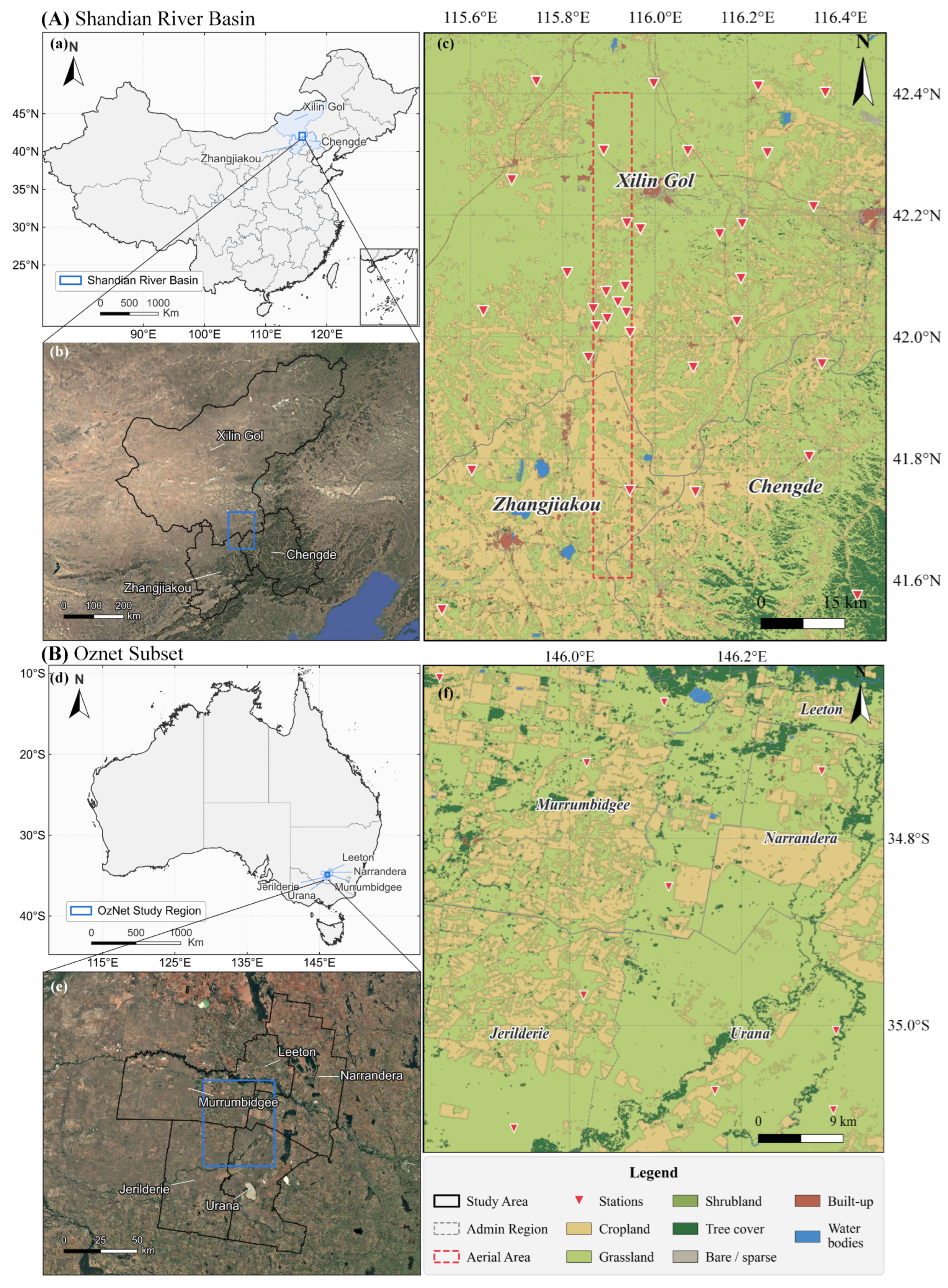
This study evaluates the proposed method in the Shandian River Basin in China and in a selected subset of the OzNet network in Australia, as shown in Figure 1. The Shandian River Basin serves as the modeling and primary evaluation region, whereas the OzNet subset is used for a stability test under direct transfer. In this test, the parameterization calibrated in the Shandian River Basin was applied to OzNet without local recalibration.
The Shandian River Basin has been used in recent field experiments and dataset evaluations for microwave soil moisture studies [35,36]. It represents a transition zone between relatively dry and wet surface conditions. Land cover is heterogeneous, with widespread grassland and cropland, together with tree cover and bare or sparsely vegetated surfaces. This setting provides a suitable testbed for evaluating retrieval performance under mixed land-cover conditions.
The OzNet region considered in this study is located in the semi-arid Murrumbidgee catchment in Australia [37]. It is also a well-established evaluation region in microwave soil moisture studies [28,38]. The selected OzNet subset was taken from a spatially coherent part of the network with relatively continuous in situ records and sufficient Sentinel-1/SMAP collocations during the study period. The subset includes both cropland and natural vegetation backgrounds. Therefore, the OzNet experiment should be interpreted as a direct-transfer stability test under comparable semi-arid cropland–grassland conditions, rather than as evidence that the proposed framework is universally applicable across all climate regimes.

2.2. Data Sources and Preprocessing

2.2.1. Sentinel-1 and NDVI

The Sentinel-1 satellite is equipped with a C-band SAR instrument. Its GRD products provide dual-polarized backscatter observations (VV and VH) at 10 m spacing, with a nominal revisit interval of 12 days per satellite. In this study, Sentinel-1 GRD data acquired in interferometric wide swath (IW) mode with VV and VH polarizations were used.
The method was evaluated in two independent study areas. A total of 82 descending-orbit Sentinel-1B acquisitions were used for the Shandian River Basin, and 92 descending-orbit Sentinel-1A acquisitions were used for the OzNet region. Only descending-orbit observations were used to maintain consistent observation geometry and acquisition time in the change-detection time series. Radar preprocessing was implemented on the Google Earth Engine (GEE) platform. The Sentinel-1 GRD collection in GEE includes standard procedures such as thermal noise removal, radiometric calibration, and terrain correction. Additional processing included speckle filtering [39] and incidence-angle normalization [34]. Before aggregation to 100 m, the 10 m Sentinel-1 VV samples were screened using a fixed backscatter plausibility range of −30 to −4 dB after daily mosaicking and incidence-angle normalization. In the Shandian River Basin, this screening removed 4.38% of the valid VV pixel–date samples, and the remaining samples were aggregated to the 100 m grid using arithmetic averaging.
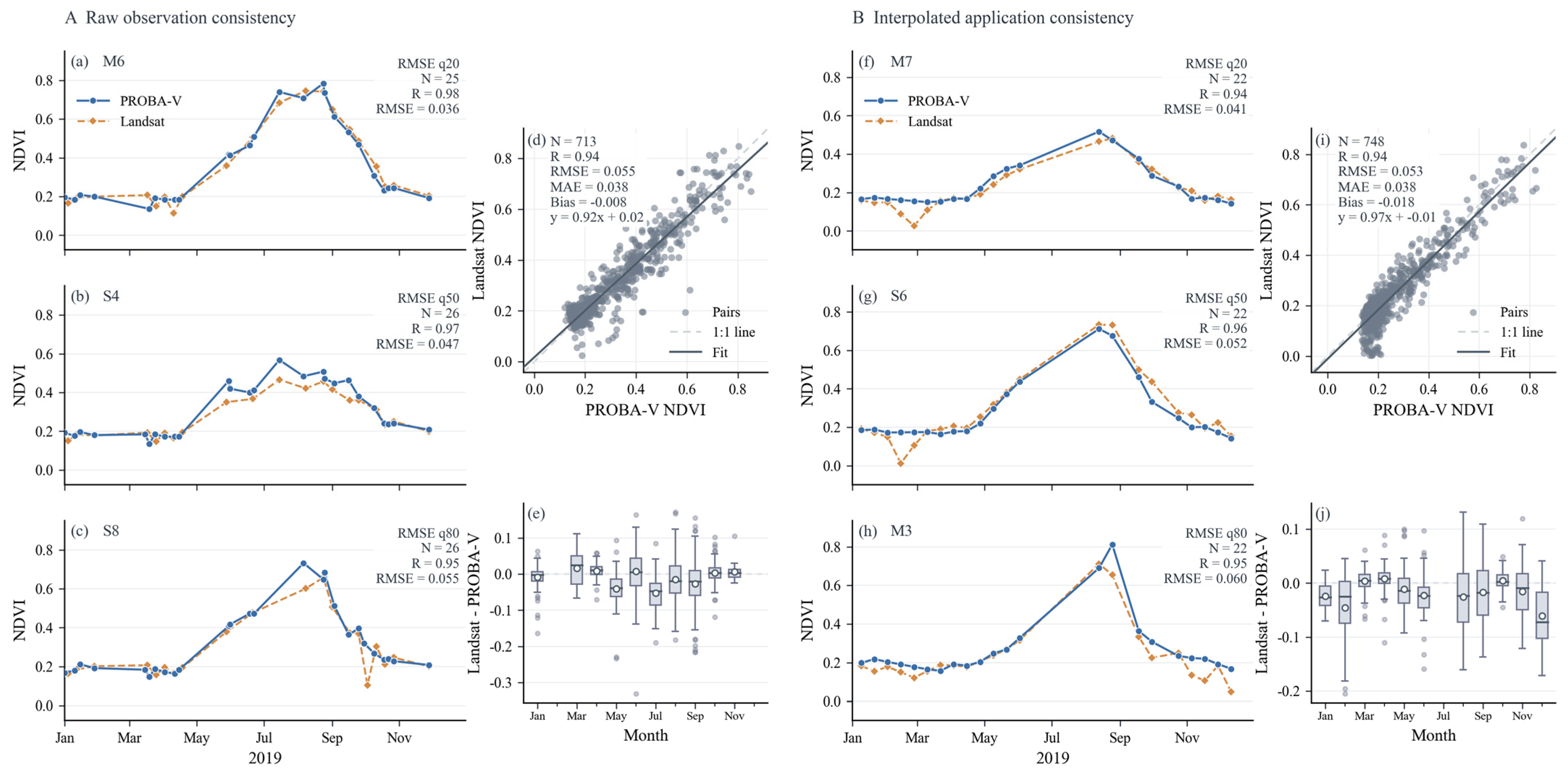
NDVI was primarily derived from the PROBA-V C1 Top-of-Canopy Daily Synthesis product at 100 m resolution in GEE. NDVI values were constrained to the range of 0–0.92 to reduce contamination from water bodies and non-vegetated surfaces. Because the operational PROBA-V products were discontinued in June 2020, NDVI after 2020 was derived from Landsat imagery due to persistent cloud contamination in Sentinel-2 observations over the study areas. The Landsat-based NDVI was aggregated to 100 m using mean resampling. Both NDVI time series were linearly interpolated at the pixel level to match the Sentinel-1 acquisition dates. In this study, NDVI was used as a practical proxy for vegetation condition rather than as a core output of the framework. Because the NDVI series was assembled from both PROBA-V and Landsat, additional overlap-period analyses were conducted to examine the consistency between the two sources and the possible influence of sensor transition on the retrieval chain.

2.2.2. SMAP and SMAP-Based Datasets

Coarse-scale soil moisture was obtained from the Soil Moisture Active Passive (SMAP) SPL3SMP_E product at 9 km resolution [6]. This product provides soil moisture estimates retrieved at ~33 km and regridded to 9 km, with a temporal sampling of 2–3 days [40].
Two additional SMAP-based soil moisture products were used for product-scale comparison. These products included the SMAP-derived 1 km downscaled surface soil moisture product (V001) [41] and the SMAP/Sentinel-1 L2 radiometer/radar 3 km EASE-Grid soil moisture product (Version 3) [29,30]. The former represents a passive-microwave downscaling product, whereas the latter provides an operational SMAP/Sentinel-1 high-resolution soil moisture product. These products were used to examine whether ISSF produced reasonable temporal behavior and spatial patterns relative to existing SMAP-based products, rather than as strict ground-truth references. All SMAP-based datasets were obtained from the NASA National Snow and Ice Data Center (NSIDC). For scale-consistent comparison, the 100 m ISSF retrievals were aggregated to the grid scale of each comparison product using arithmetic averaging.

2.2.3. Auxiliary Datasets and Evaluation Data

Daily precipitation was obtained from the CHIRPS Daily product (Version 2.0 Final) [42]. CHIRPS combines satellite observations at 0.05° resolution with gauge measurements to produce gridded daily precipitation time series. The dataset was accessed through the GEE platform.
MODIS evapotranspiration data were used only in the DSCALE_mod16-based moisture-anchoring-scale sensitivity test. The MODIS/Terra Net Evapotranspiration Gap-Filled 8-Day L4 Global 500 m product (MOD16A2GF, Version 6.1) was used to calculate land surface evaporative efficiency as the ratio of evapotranspiration to potential evapotranspiration [43]. This variable was then used by DSCALE_mod16 to generate alternative fine-scale dry/wet moisture anchoring intervals. This dataset was not used in the default ISSF retrieval chain.
Land cover information was obtained from the ESA WorldCover 2020 map at 10 m resolution. This product is derived from Sentinel-1 and Sentinel-2 data and includes 11 land-cover categories [44]. The dataset was accessed through the GEE platform.
In situ soil moisture measurements for both study areas were obtained from the International Soil Moisture Network (ISMN). Observations at 0–5 cm depth were used in the analysis. The original measurements (10-min for the Shandian River sites and hourly for the OzNet sites) were aggregated to overpass-scale values by averaging the records within ±1 h of the Sentinel-1 overpass time. Records outside the physical range (0–0.6 m3/m3) and those flagged by quality control were removed. The in situ observations were then temporally matched to Sentinel-1 acquisition dates for validation.
The airborne observation was acquired on 24 September 2018 during a comprehensive field campaign in the Shandian River Basin [35,36]. The flight covered approximately 70 km × 12 km. It provided coincident L-band active-passive microwave observations, including L-band radiometer observations at 1 km resolution. The airborne acquisition was conducted on 24 September, whereas the corresponding Sentinel-1 overpass occurred on 23 September. Local meteorological records indicated no precipitation during the intervening 24-h period, suggesting that surface soil moisture conditions remained stable between the satellite and airborne acquisitions.

3. Method

3.1. Overview of the Improved Sentinel-1 Change-Detection Method

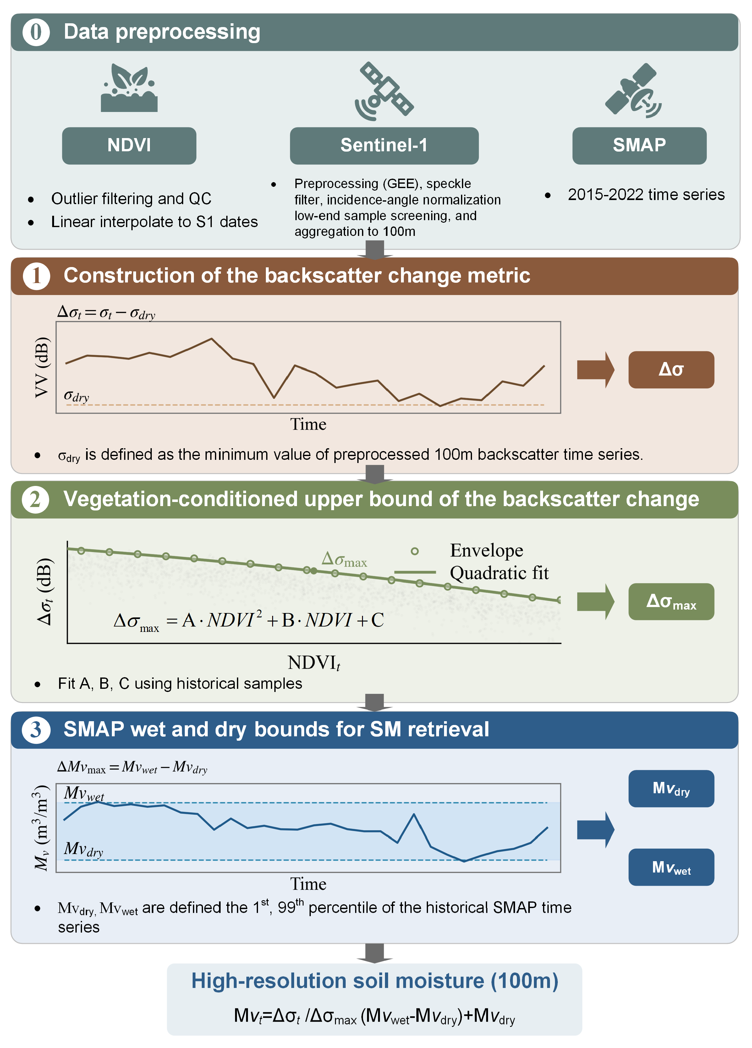
Figure 2 shows the improved SMAP-anchored Sentinel-1 change-detection framework (ISSF). ISSF follows the Sentinel-1 change-detection route, in which temporal changes in VV backscatter are used to describe fine-scale wetting and drying dynamics. Two constraints are introduced to convert this relative change signal into 100 m volumetric surface soil moisture. The first is a vegetation-conditioned dynamic-range constraint, which uses an NDVI-based upper-bound model to account for the reduction in the observable backscatter-change range under different vegetation conditions. The second is a SMAP-based moisture-anchoring constraint, which uses multi-year SMAP dry/wet bounds to scale the normalized Sentinel-1 relative wetness into volumetric soil moisture. In this design, Sentinel-1 provides the fine-scale temporal change information, while SMAP provides the coarse-scale volumetric reference.

3.1.1. Construction of the Backscatter Coefficient Change Metric

The change detection method assumes that temporal variations in surface roughness are small relative to moisture-driven backscatter coefficient changes. Under this assumption, temporal variations in backscatter coefficient can be used to describe soil moisture dynamics [20,28]. For each 100 m pixel, a backscatter coefficient time series was constructed from the preprocessed Sentinel-1 observations. A dry reference signal was then defined from this 100 m time series as follows:
σ dry = ( { σ t } t T ) min
where σ dry is the dry reference of the backscatter coefficient time series { σ t } t T . In this study, data from 2018–2019 were selected for calculation. ( ) min denotes the function used to compute the minimum value. The backscatter coefficient change at date t is then defined as:
Δ σ t = σ t σ dry
where σ t is the Sentinel-1 VV backscatter coefficient at date t . Under stable surface and vegetation conditions, backscatter coefficient changes are often approximately proportional to soil moisture changes. This relation provides the basis for tracking wetting and drying from temporal variations in backscatter coefficient [21,45]. Based on this relation, the following expression is obtained:
Δ σ t Δ σ max = Δ M v t Δ M v max
where Δ σ t denotes the backscatter coefficient change at time t relative to the dry reference. Δ σ max is upper bound of observable backscatter coefficient change. Δ M v t is the change in volumetric soil moisture at time t relative to the dry bound. Δ M v max represents the maximum range of soil moisture variation.

3.1.2. Vegetation-Conditioned Upper Bound of the Backscatter Change

The key issue addressed in this section is that the observable range of soil-moisture-related backscatter change is not constant across vegetation conditions. In vegetated areas, the observed backscatter coefficient σ obs can be described by the water cloud model (WCM) as the sum of the vegetation volume scattering term σ veg and the attenuated soil scattering term [46,47].
σ obs = σ veg + τ 2 σ soil
τ 2 = exp ( 2 A WCM VI / cos θ )
where σ obs is the observed backscatter coefficient. σ veg is the vegetation volume scattering term, and σ soil is the soil scattering term. τ 2 denotes the two-way vegetation transmissivity. A WCM is an empirical coefficient that depends on radar configuration and vegetation type, and VI represents an aggregated vegetation descriptor, for example leaf area index (LAI), vegetation water content (VWC), or NDVI [48,49]. These equations indicate that vegetation attenuation reduces the visibility of the soil scattering term, while vegetation volume scattering adds a background contribution. As vegetation attenuation increases, the observable backscatter-change range associated with soil moisture variation is expected to decrease.
Based on this vegetation-attenuation mechanism, the dependence of the maximum observable backscatter change on vegetation condition was estimated from the calibration samples. NDVI was used as a practical proxy for vegetation condition:
NDVI = NIR R NIR + R
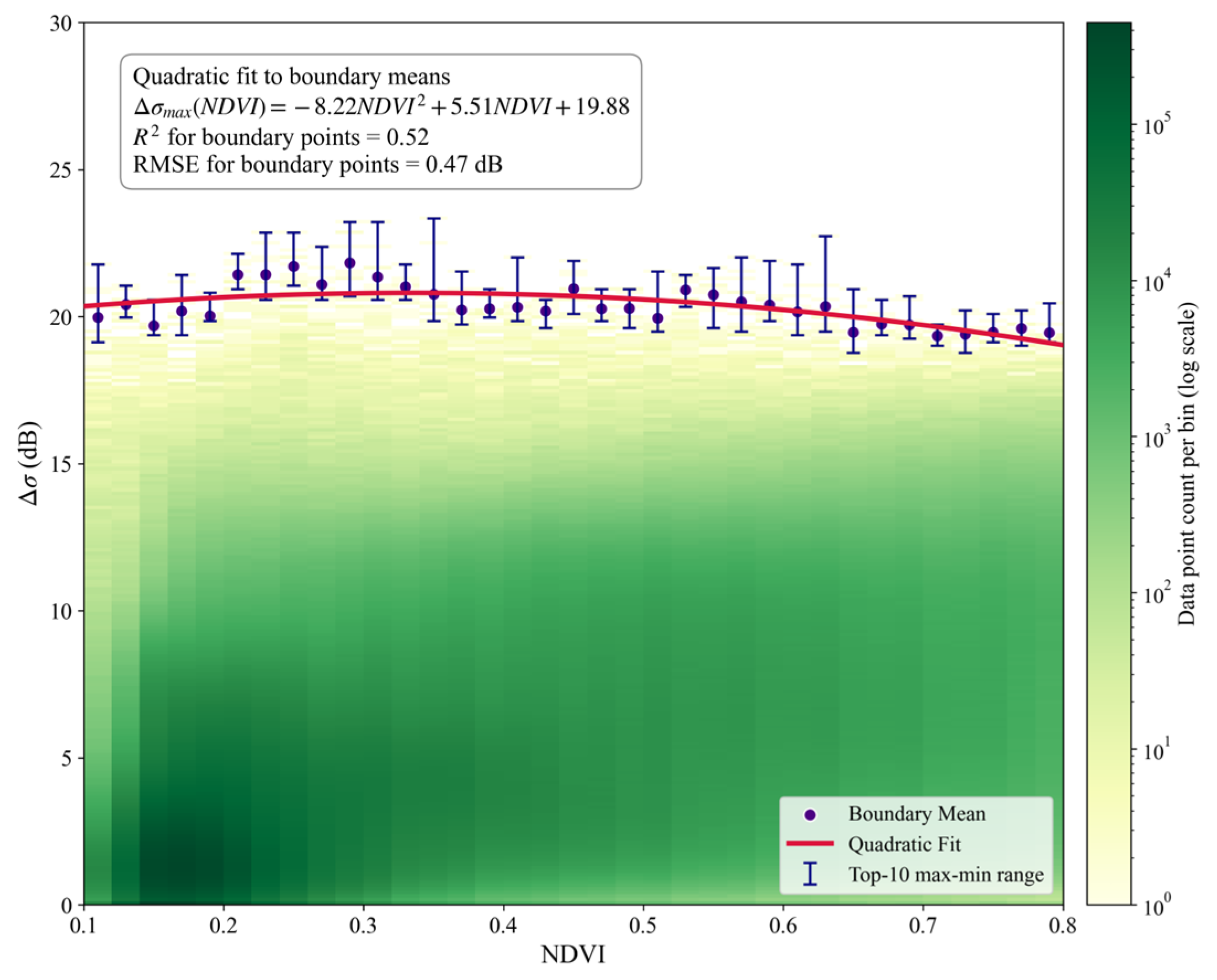
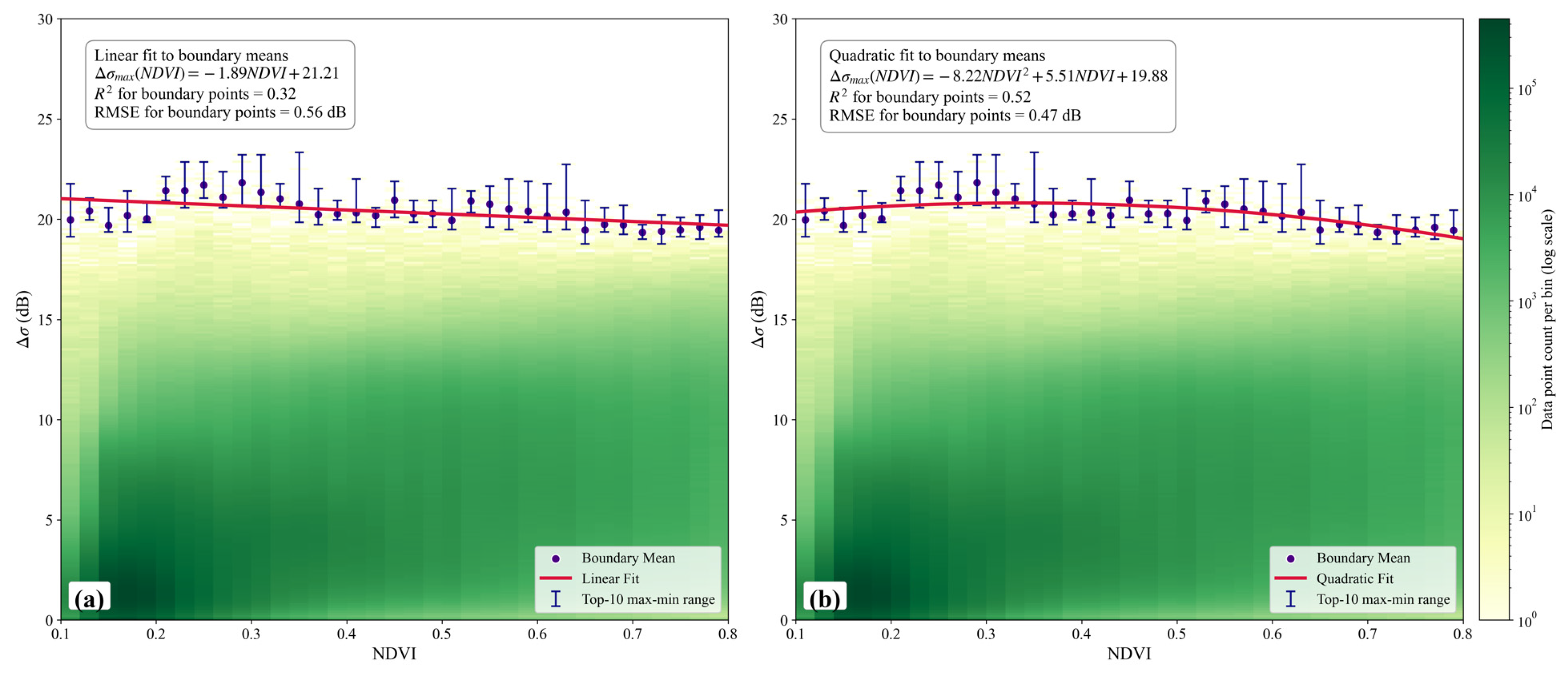
where NIR and R denote the reflectance values in the near-infrared and red bands, respectively. Historical Sentinel-1 and NDVI observations from the calibration period were used to extract the upper envelope of the Δ σ NDVI distribution. Water bodies and dense forests were excluded, and valid samples were restricted to NDVI values between 0 and 0.8. NDVI was binned at an interval of 0.02. In each bin, the mean of the top 10 largest backscatter-change values was used as the bin-wise upper-bound sample. The Top-10 setting was used as a practical compromise between preserving the upper-envelope signal and reducing sensitivity to individual extreme values, and its influence was examined in the sensitivity analysis in Section 4.4.1. The extracted upper-bound samples showed a nonlinear dependence on NDVI. Therefore, a second-order polynomial was fitted to these samples:
Δ σ max ( NDVI ) = A NDVI 2 + B NDVI + C
where A , B , and C are fitted parameters. The fitted function was used to estimate the vegetation-conditioned maximum observable backscatter-change range for each 100 m pixel and Sentinel-1 acquisition date (Figure 3):

3.1.3. SMAP Wet and Dry Bounds for SM Retrieval

The change-detection metric describes relative wetness variations rather than absolute soil moisture. Converting this relative metric into volumetric soil moisture therefore requires dry and wet reference bounds. Rather than using one regional pair of bounds for the entire study area, this framework defines dry and wet anchors separately for each SMAP grid cell. The soil moisture dynamic range is defined as follows:
Δ M v max = M v wet M v dry
where M v wet , M v dry represent the wettest and driest soil moisture values for each SMAP 9-km grid cell. The resulting bounds are defined at the SMAP grid-cell scale and assigned to all 100-m pixels within the same grid cell. For each SMAP grid cell, the following quantities are defined:
M v dry = Q 0.01 ( { SMAP t } t = 1 T )
M v wet = Q 0.99 ( { SMAP t } t = 1 T )
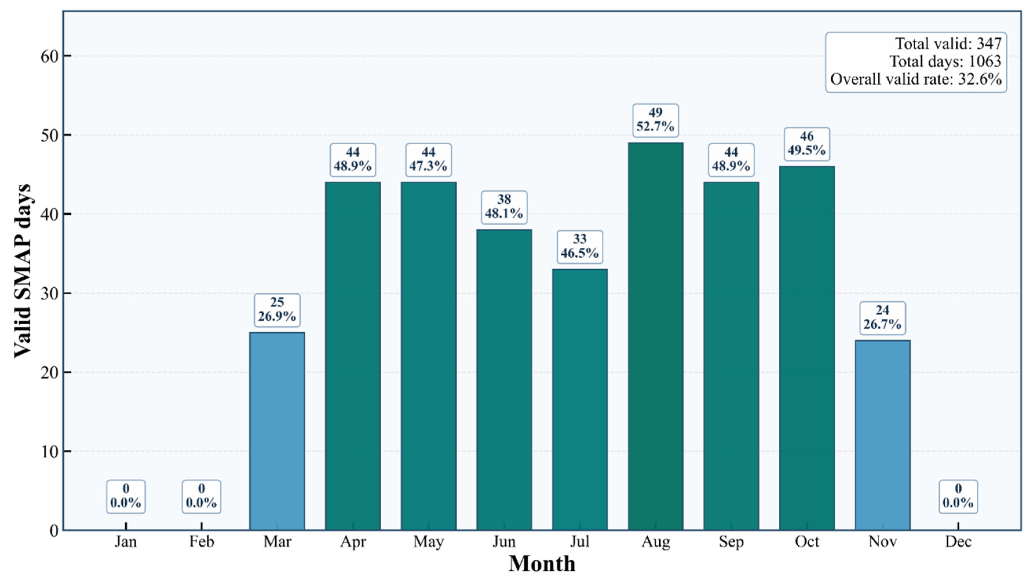
where Q 0.01 ( ) , Q 0.99 ( ) denote the functions that compute the 1st and 99th percentiles, respectively. In this study, the dry and wet bounds were estimated from the full available SMAP record (2015–2022) using the 1st and 99th percentiles in order to reduce the influence of outliers. The full 2015–2022 SMAP record was used to define an empirical dry–wet dynamic range for each SMAP grid cell, rather than to assume stationary annual moisture conditions. The 1st and 99th percentiles were selected to reduce the influence of isolated extremes while retaining the long-term dry and wet states observed by SMAP. The influence of reference-period length and quantile choice was examined in Appendix A. The estimation of dry and wet bounds relies on the multi-year SMAP time series. The SMAP Enhanced L3 processor applies quality control for frozen conditions based on effective soil temperature. Soil moisture retrievals are masked when the frozen area fraction is high. An analysis of monthly SMAP data availability in the study area showed that almost no valid data were available during January, February, late November, and December. Therefore, deep-winter frozen samples were effectively excluded from the M v wet , M v dry estimation.
The overall retrieval equation is then written as follows:
M v t = Δ σ t A NDVI 2 + B NDVI + C Δ M v max + M v dry
To keep the retrievals physically consistent with the predefined dry–wet interval, values lower than the dry bound were set to the dry bound, and values higher than the wet bound were set to the wet bound.

3.2. Evaluation and Sensitivity Analysis Design

A multi-level evaluation and sensitivity analysis design was used to assess the default ISSF configuration and to diagnose the robustness of its two key constraints. Point-scale validation was first conducted using in situ measurements. Area-scale spatial consistency was then evaluated using a near-concurrent airborne reference and spatial texture diagnostics. Two additional sensitivity tests were designed to examine whether the two constraint terms were sensitive to the choice of vegetation proxy and the spatial scale of moisture anchoring. Finally, a stability test under direct transfer was conducted over the OzNet subset to examine whether the calibrated parameterization remained stable when applied to a comparable semi-arid cropland–grassland region without local recalibration.

3.2.1. Point-Scale Evaluation

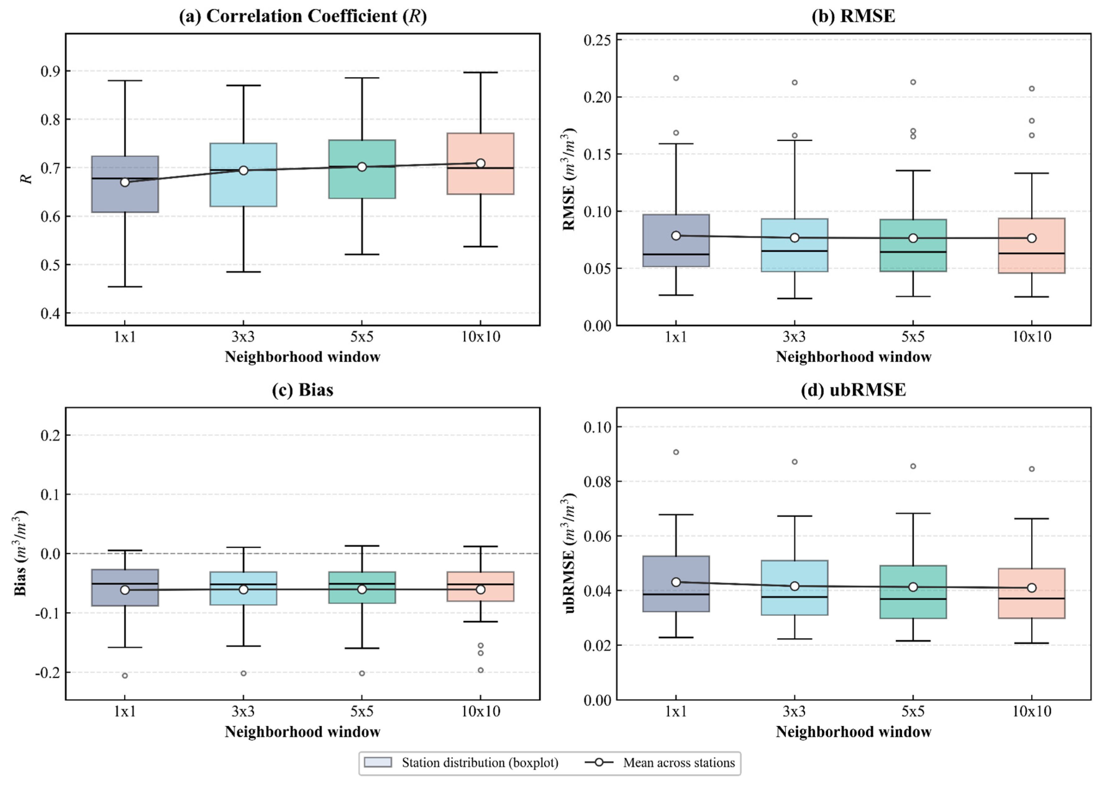
Point-scale evaluation was conducted using 0–5 cm in situ soil moisture measurements from the Shandian River Basin. The in situ measurements were used as the reference and were temporally matched to Sentinel-1 acquisition dates. Because the in situ measurements were point-based whereas the ISSF retrieval was reported at 100 m, a neighborhood-scale sensitivity analysis was conducted around each station to examine the influence of point-to-pixel representativeness error on the evaluation statistics. ISSF retrievals were averaged over 1 × 1, 3 × 3, 5 × 5, and 10 × 10 pixel windows centered on each station, and the corresponding evaluation statistics were compared.
ISSF was further compared with three representative Sentinel-1-based change-detection baselines, including Gao et al. [27], Du et al. [34], and short-term change detection (STCD) [50]. These baseline methods were selected to represent related but distinct retrieval routes within the Sentinel-1 change-detection family. Gao combines Sentinel-1 temporal change information with an NDVI-dependent backscatter-change range and study-area-scale moisture bounds constrained by coarse-scale SMOS information. Du also follows a Sentinel-1 change-detection strategy, but converts relative wetness to volumetric soil moisture using dry/wet bounds fitted for the target setting. STCD was included as a recent baseline within the same methodological family.
All methods used Sentinel-1 VV backscatter in dB as the primary input. The comparison applied the same spatial masks, including the removal of water bodies and dense forests. Other empirical settings and constants followed the original studies. Evaluation metrics included bias, Pearson correlation coefficient (R), root-mean-square error (RMSE), and unbiased RMSE (ubRMSE). ubRMSE was used to assess the ability to represent temporal soil moisture variations after removing systematic bias. The metrics are defined as follows:
R = ( θ o E [ θ o ] ) ( θ r E [ θ r ] ) ( θ o E [ θ o ] ) 2 ( θ r E [ θ r ] ) 2
Bias = 1 n i = 1 n ( S o , i θ r , i )
RMSE = E [ ( θ o θ r ) 2 ]
ubRMSE = E [ ( θ o E [ θ o ] ) ( θ r E [ θ r ] ) 2 ]
where E ( ) denotes the mean of the data in brackets, and θ o , θ r denote the retrieved and reference soil moisture values, respectively.

3.2.2. Area-Scale Spatial Evaluation

Area-scale spatial evaluation was conducted using a near-concurrent 1 km soil moisture product retrieved from an airborne L-band radiometer. The airborne map was used as an event-scale regional reference to examine whether ISSF could reproduce the wet–dry gradient and spatial texture for the available airborne event.
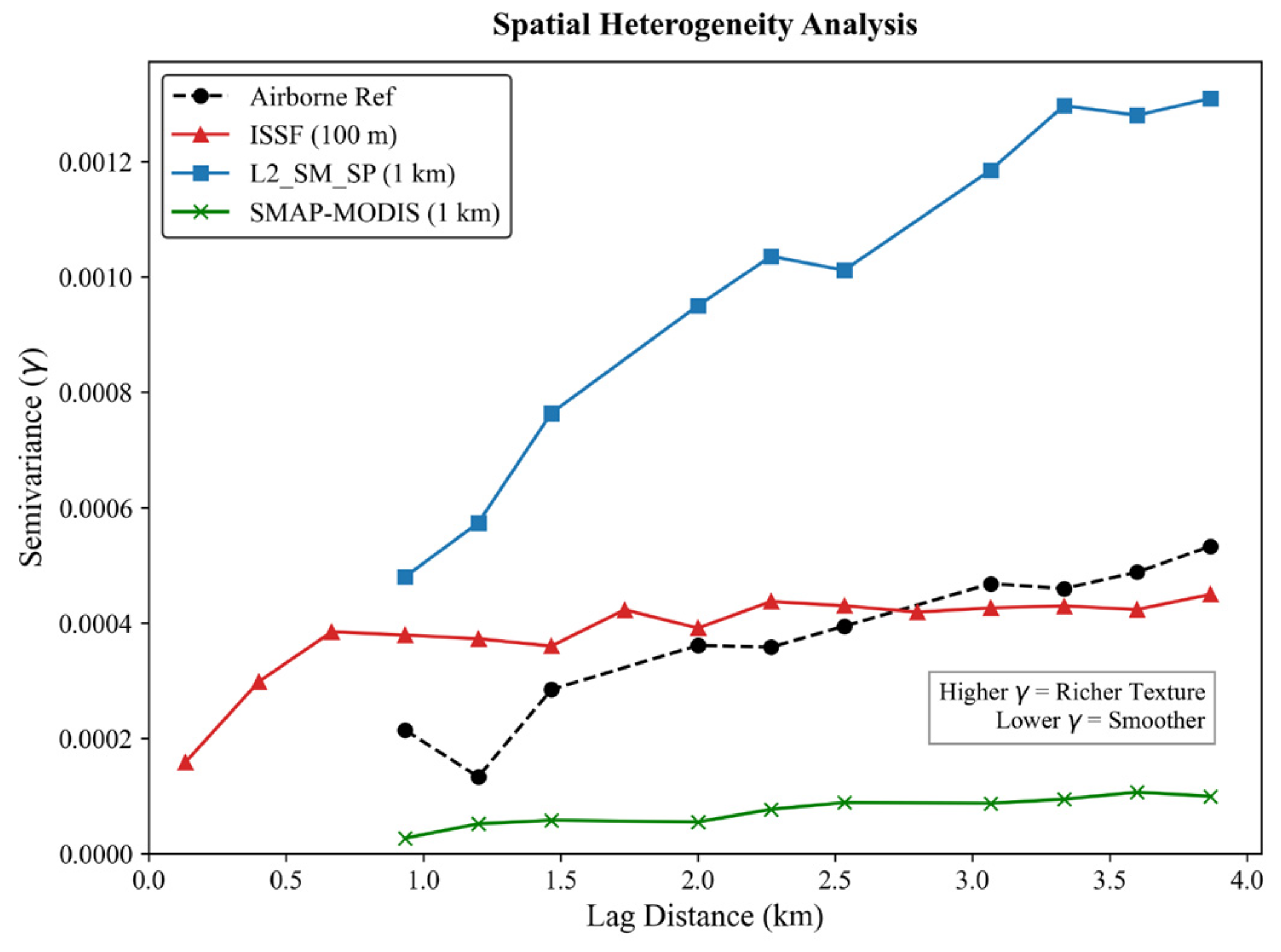
Spatial texture was further examined using the experimental semivariogram. Semivariogram-based analysis and related spatial-structure diagnostics have been widely used to characterize the scale-dependent spatial dependence of soil moisture and to support the evaluation of high-resolution soil moisture products, especially when point-scale metrics alone cannot describe regional spatial organization. The semivariogram of the airborne product was treated as an event-based regional reference. The experimental semivariogram is defined as follows [51,52]:
γ ( h ) = 1 2 N ( h ) i = 1 N ( h ) Z ( x i ) Z ( x i + h ) 2
where γ ( h ) is the semivariance at lag distance h , N h is the number of point pairs, and Z x i is the soil moisture value at location x i . Experimental semivariograms were computed for lag distances from 0 to 4 km, which match the typical scale of grassland-cropland patches in the study area. Because the 100 m and 1 km products differ in pixel density, random sampling was used for the 100 m products, whereas all valid pixels were used for the 1 km products. This design ensured robust estimation of spatial variability.

3.2.3. Constraint Sensitivity Analysis

The diagnostic sensitivity analyses were conducted to examine the robustness of the two key constraints in ISSF. The first analysis examined the sensitivity to the vegetation-conditioned upper-bound representation. The second analysis examined the influence of vegetation information source and proxy selection. The third analysis examined the effect of SMAP-based moisture anchoring and boundary scale.
  • Sensitivity to vegetation-conditioned upper-bound representation
The first test compared the fixed upper-bound scheme with the NDVI-conditioned quadratic upper-bound scheme to examine whether a vegetation-dependent dynamic range improved the normalization of Sentinel-1 backscatter changes.
  • Sensitivity to vegetation proxy selection
NDVI was used as the default vegetation proxy in ISSF because it directly represents green vegetation cover. However, optical vegetation observations can be affected by cloud contamination, temporal interpolation, and sensor transitions. Therefore, RVI was tested as a radar-based alternative vegetation proxy. In this test, only the vegetation proxy was replaced, whereas the upper-envelope extraction strategy, the Sentinel-1 relative wetness calculation, and the SMAP-based moisture anchoring scheme were kept unchanged.
RVI was calculated from Sentinel-1 VV and VH backscattering intensities as [53,54]:
RVI = 4 σ VH σ VV + σ VH
where σ VV is the backscattering coefficient of VV polarization. σ VH is the backscattering coefficient of VH polarization. RVI is based on the linear scattering intensities of co-polarization and cross-polarization and typically ranges from 0 to 1.
  • Sensitivity to moisture-anchoring scale
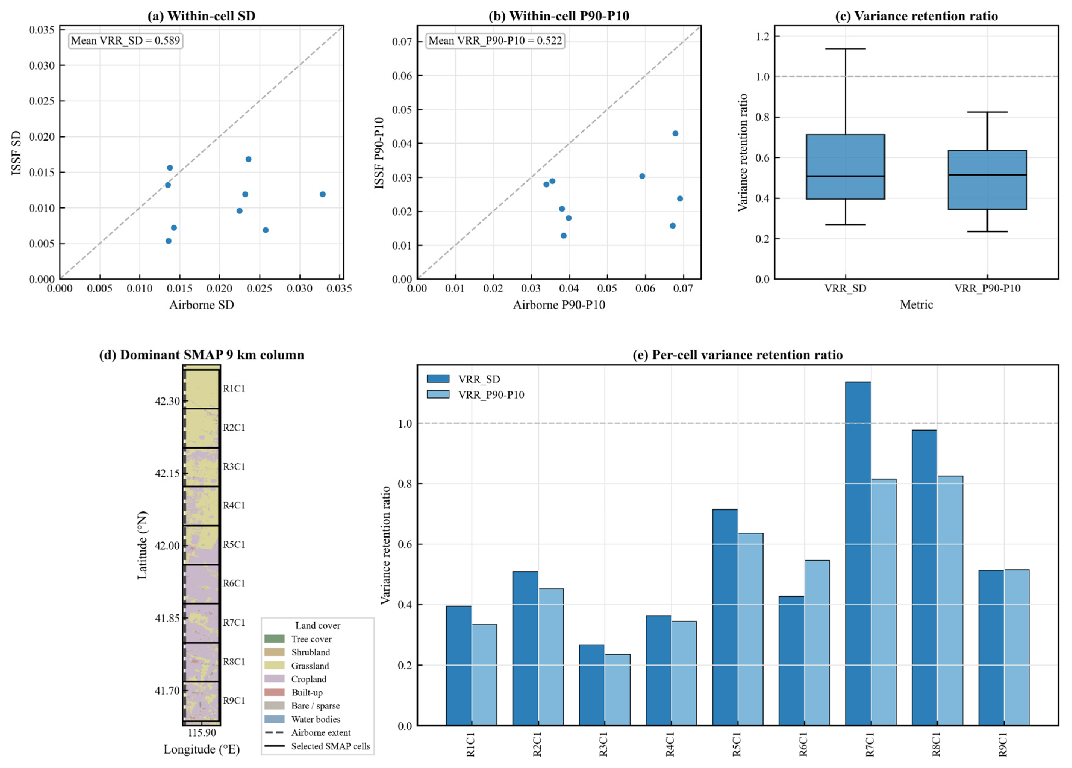
Within selected SMAP 9 km cells, sub-grid variability was further assessed by comparing the within-cell spatial dispersion of the airborne 1 km reference and the ISSF retrieval aggregated to 1 km. In this analysis, the variability retention ratio (VRR) was quantified using both the within-cell standard deviation and the P90-P10 range, where P90 and P10 denote the 90th and 10th percentiles of the within-cell soil moisture distribution, respectively.
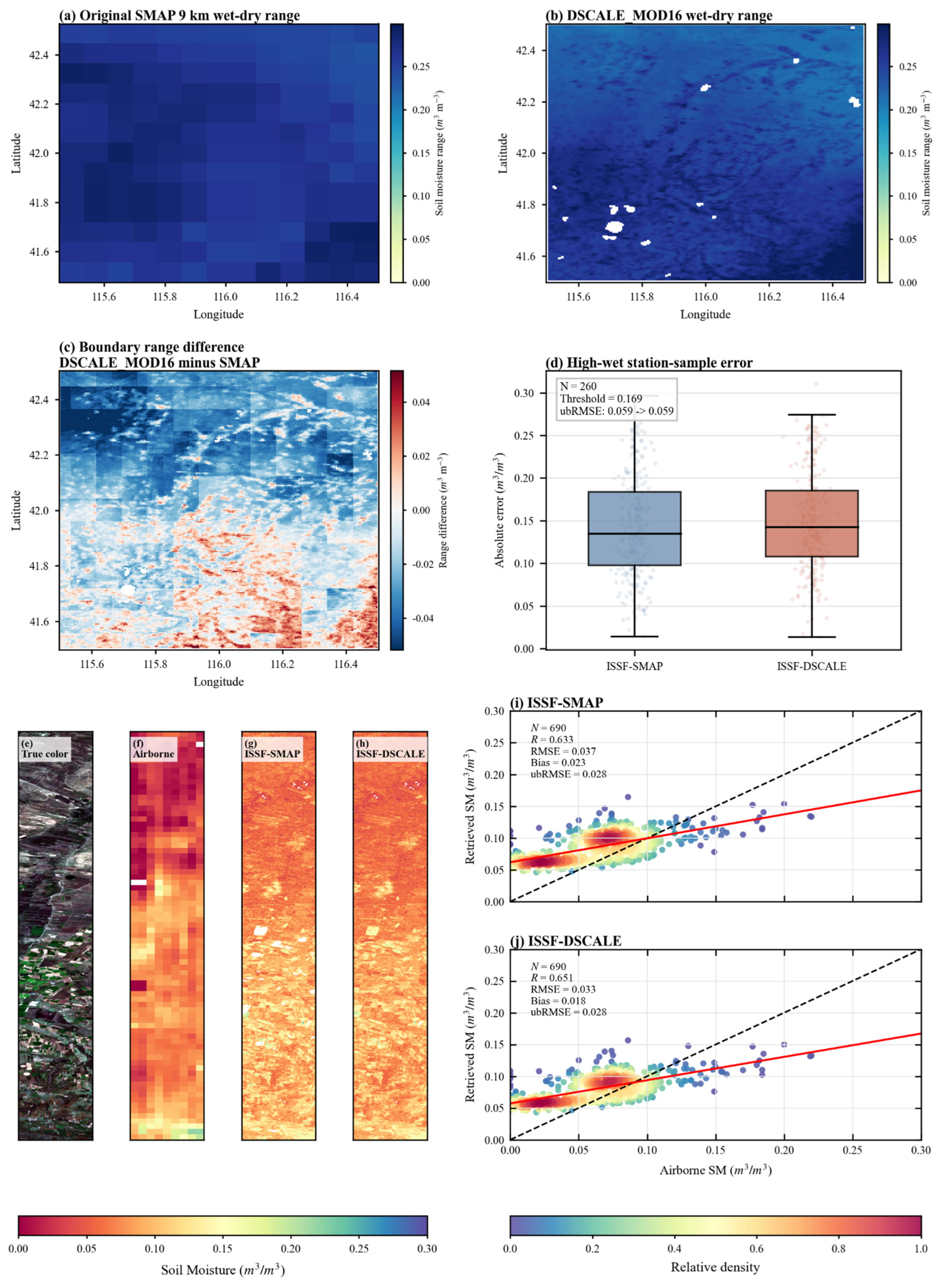
The original SMAP 9 km dry/wet anchoring interval was used as the default moisture-anchoring scheme in ISSF. Because coarse-scale anchoring may smooth sub-grid wet–dry variability, a sensitivity test was conducted using DSCALE_mod16-downscaled SMAP soil moisture. DSCALE_mod16 is a microwave soil moisture downscaling method that uses land surface evaporative efficiency derived from MODIS evapotranspiration products and meteorological data as the main downscaling factor [55]. In this study, DSCALE_mod16 was used only to generate an alternative finer-scale moisture anchoring interval. It was not used to replace the Sentinel-1 change-detection component.
Specifically, the Sentinel-1-derived relative wetness and the NDVI-based vegetation-conditioned upper-bound function were kept unchanged. The DSCALE_mod16-downscaled SMAP time series was used to estimate alternative dry and wet anchors using the 1st and 99th percentiles. This test was designed to examine whether a finer-scale passive-microwave anchoring interval could reduce wet-end errors or improve sub-grid variability retention.

3.2.4. Within-Domain Direct-Transfer Test

A stability test under direct transfer was conducted over the OzNet subset in Australia. The vegetation-conditioned upper-bound relation calibrated in the Shandian River Basin was directly applied to OzNet without local recalibration. OzNet in situ measurements were used as the reference. This test was designed to assess the behavior of the Shandian-calibrated parameterization when applied, without local recalibration, to a second region with comparable semi-arid cropland–grassland conditions. It therefore evaluates within-domain transfer stability, rather than broad geographic generalization.

4. Results

4.1. Point-Scale Evaluation and Benchmark Comparison

4.1.1. Overall Point-Scale Comparison

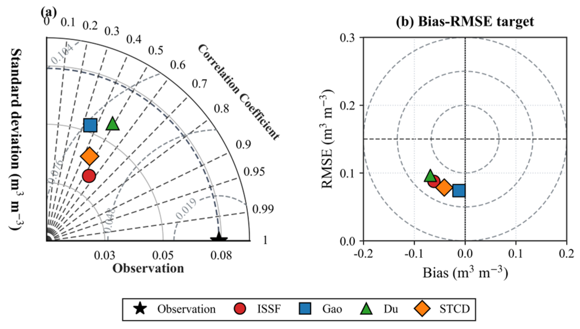
Figure 4 summarizes the overall point-scale performance of ISSF and the benchmark change-detection methods during the modeling period. In the Taylor diagram, ISSF is located closest to the observation reference, indicating a favorable balance among correlation, variability, and centered error. In the target diagram, Gao shows the smallest systematic bias, whereas ISSF shows lower unbiased error and more stable temporal agreement. Compared with Gao, Du, and STCD, ISSF increased R by 52.69%, 11.21%, and 20.77%, respectively, and reduced ubRMSE by 14.60%, 8.34%, and 7.10%, respectively. Overall, ISSF provides the most balanced performance among the tested change-detection methods, although no single method is uniformly superior across all metrics.

4.1.2. Temporal Stability Between Modeling and Evaluation Periods

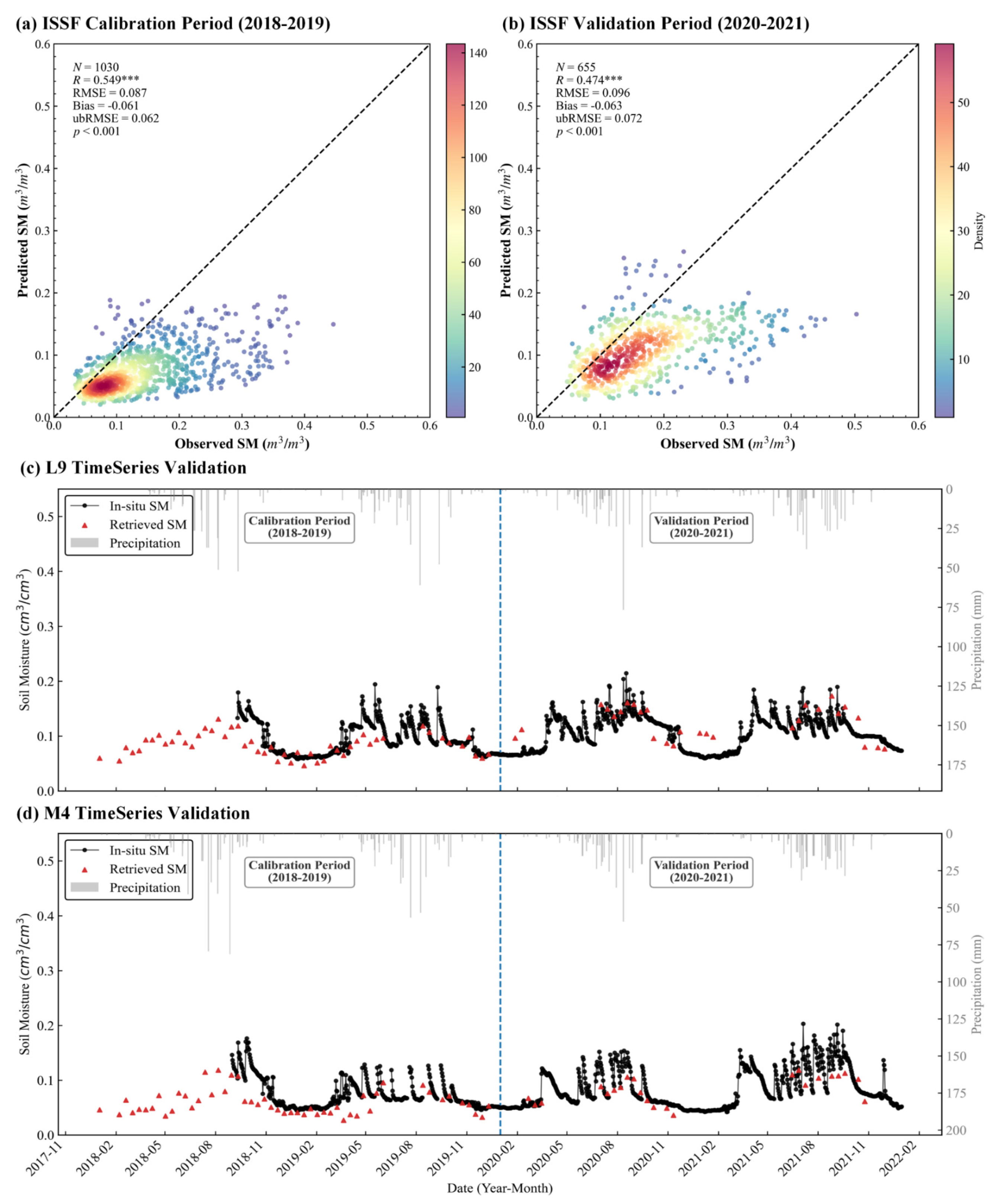
To evaluate robustness beyond the modeling period, Figure 5 compares performance in the modeling period (2018–2019) and the validation period (2020–2021). In both periods, the high-density region remains aligned with the 1:1 line, with no evident year-to-year shift. During 2018–2019, ISSF achieved R = 0.549 and ubRMSE = 0.062 m3 m−3 using the pooled station-date samples. In the independent validation period of 2020–2021, R decreased to 0.474 and ubRMSE increased to 0.072 m3 m−3. Fisher’s r-to-z test showed that the decrease in correlation was marginally significant at the 0.05 level (z = 2.02, p = 0.043). However, the bias remained nearly unchanged between the two periods, changing from −0.061 to −0.063 m3 m−3. Thus, the validation period showed a modest reduction in the ability to track temporal variations in soil moisture, while the nearly unchanged bias suggests no clear increase in systematic underestimation or overestimation.

4.1.3. Station-Wise and Vegetation-Condition-Dependent Error Behavior

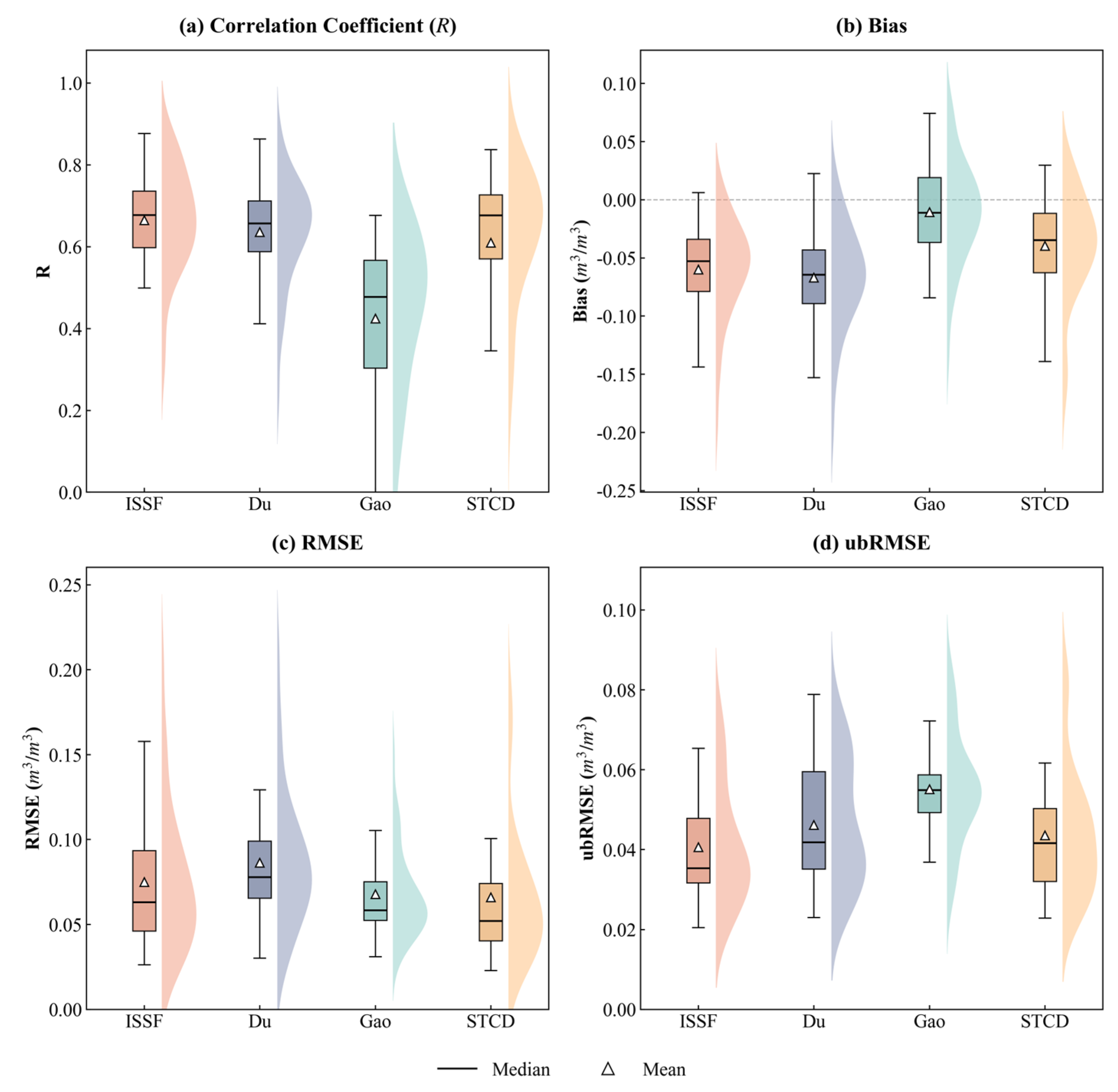
Figure 6 shows the station-wise distributions of the evaluation metrics. ISSF and STCD generally show higher station-level correlations than Gao and Du, while ISSF provides the lowest ubRMSE distribution. This indicates that the proposed constraints mainly improve the unbiased temporal component of the retrieval rather than completely removing the systematic bias.
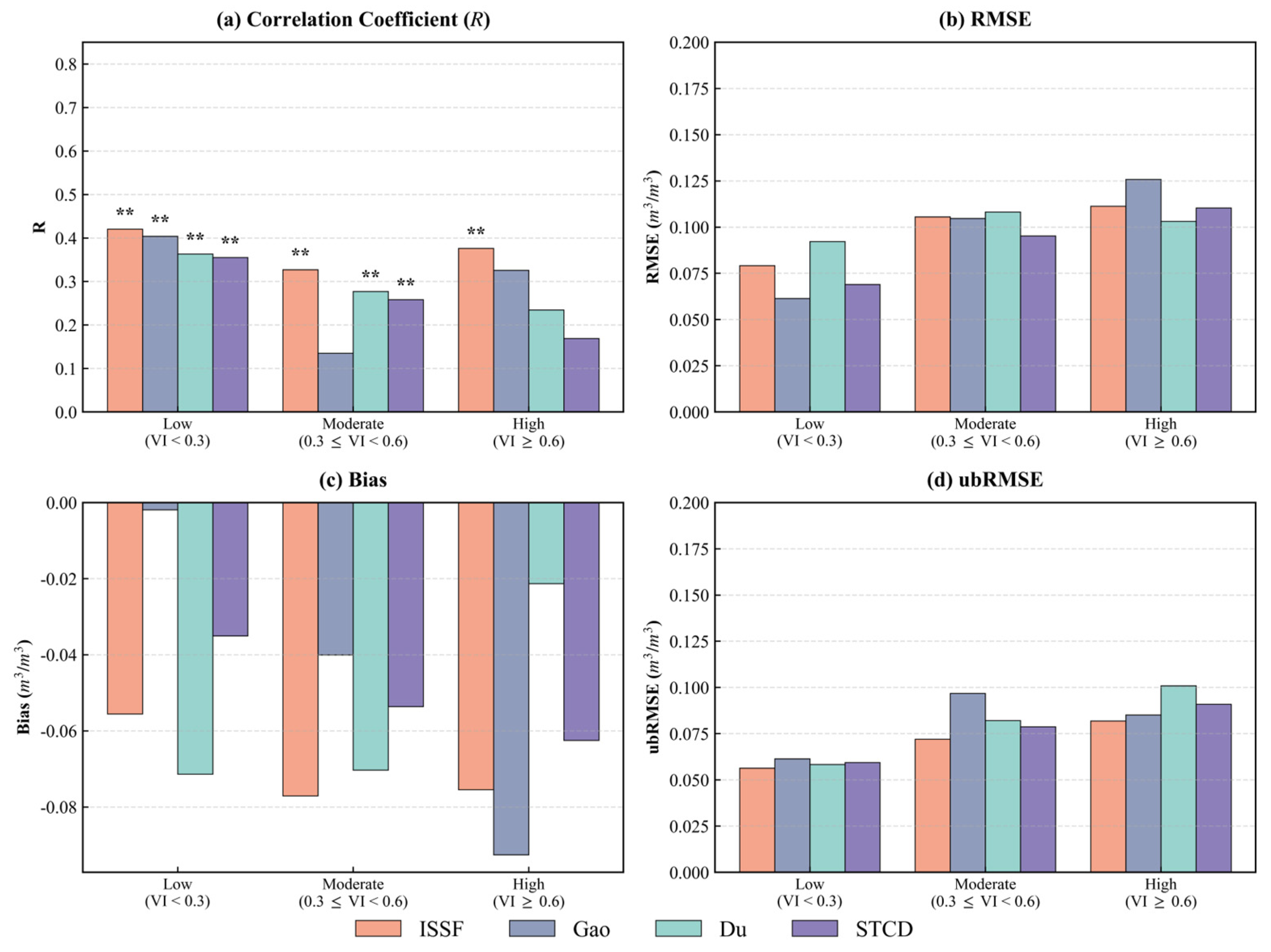
To examine how vegetation conditions affected point-scale performance, the evaluation samples were grouped into low-, moderate-, and high-vegetation classes according to NDVI. Figure 7 compares ISSF and the three benchmark methods across these vegetation classes. Overall, all methods show a decline in performance as vegetation cover increases, indicating that vegetation attenuation and volume scattering weaken the soil-moisture-related C-band response.
Under low-vegetation conditions, the differences among methods are limited. The radar response is less affected by canopy attenuation, and all methods can capture the main wetting and drying signal. ISSF shows slightly stronger temporal agreement, whereas Gao shows the smallest bias. This suggests that the vegetation-conditioned constraint provides only limited additional benefit when vegetation interference is weak.
Under moderate-vegetation conditions, the differences among methods become more evident. ISSF retained a more balanced combination of temporal agreement and unbiased error under moderate-vegetation conditions. Negative bias also becomes more evident across methods, suggesting that the observable backscatter-change range is increasingly compressed by vegetation effects.
Under high-vegetation conditions, performance decreases for all methods. ISSF still retains detectable temporal agreement and a relatively balanced error structure, but the negative bias and increased unbiased error indicate that the method does not fully overcome the reduced C-band sensitivity under denser vegetation. Therefore, the results should be interpreted as improved stability under vegetation effects rather than as a complete correction of vegetation-induced uncertainty.
In the present study, the performance degradation became more evident in the higher-vegetation group defined by NDVI ≥ 0.6. Therefore, NDVI ≈ 0.6 is used here as an empirical performance-based applicability limit for quantitative ISSF retrieval. This value should not be interpreted as a universal vegetation threshold. When NDVI exceeds this range, ISSF retrievals may still describe relative wetting and drying tendencies, but the volumetric soil moisture estimates should be interpreted with caution.
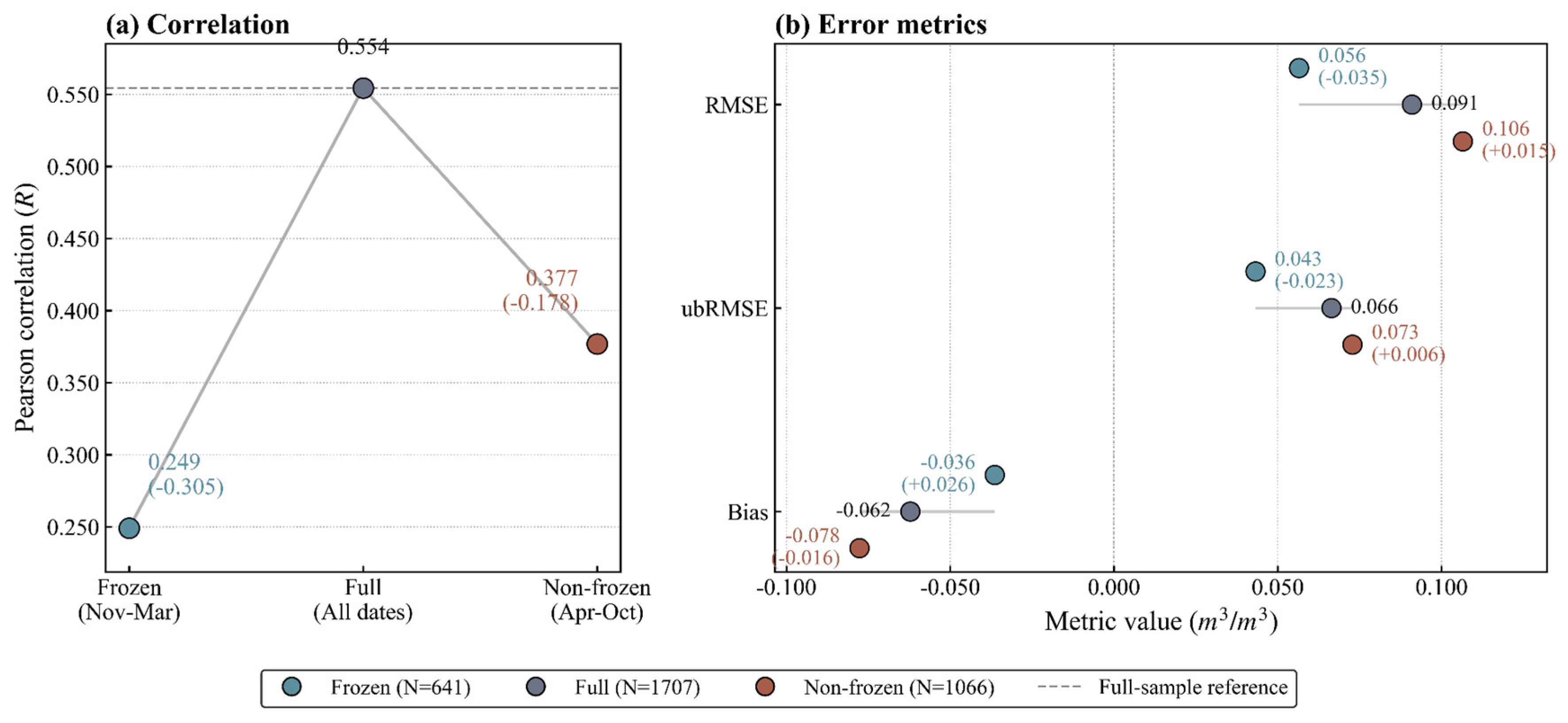
Additional grouped comparisons were used to examine whether the evaluation statistics were affected by low-variability frozen-season samples and point-to-pixel representativeness (Figure 8 and Figure 9). Excluding frozen-season samples increased the retrieval errors moderately, but the overall performance remained within a comparable range. The neighborhood-scale comparison further showed that moderate spatial averaging around the stations reduced part of the point-to-pixel mismatch, confirming the influence of representativeness error in point-scale evaluation.

4.2. Comparison with Airborne and SMAP-Based Products

4.2.1. Comparison with the Airborne Reference

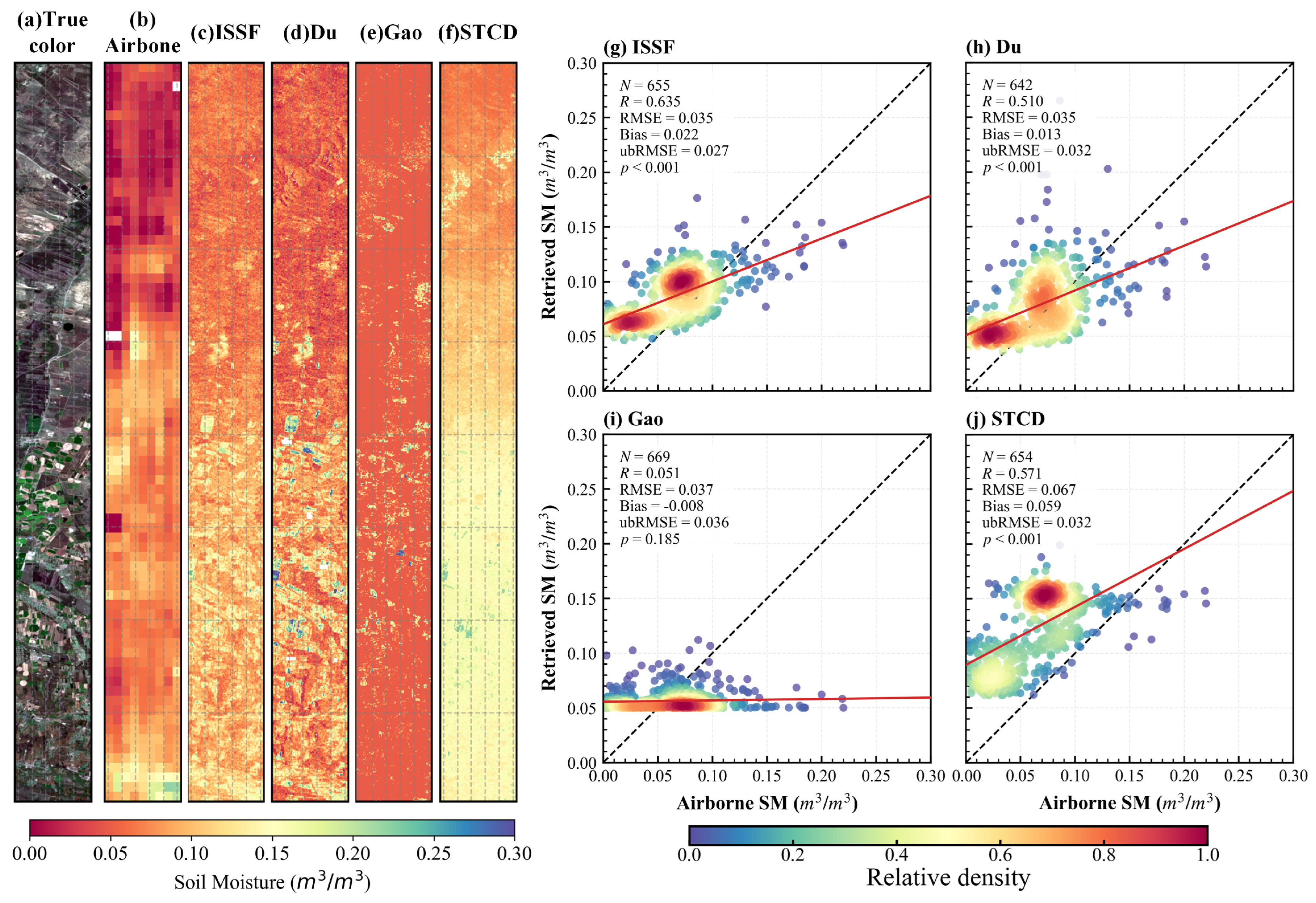
An airborne soil moisture observation was used as an event-based regional reference to compare ISSF and the baseline methods at the 1 km scale. Because only one near-concurrent airborne map was available, this comparison was used to assess event-scale spatial consistency rather than to validate general spatial performance. Figure 10a shows the true-color image of the airborne observation area. Figure 10b shows the airborne soil moisture map, which indicates generally dry conditions across the scene, with most values below 0.20 m3/m3 and a broad north–south gradient.
Figure 10c–f present the corresponding retrieval patterns from ISSF, Du, Gao, and STCD. Among the four methods, ISSF shows the closest regional pattern to the airborne reference. The density scatterplots in Figure 10g–j further quantify the area-scale comparison. ISSF shows the highest correlation and the lowest ubRMSE against the airborne reference.

4.2.2. Comparison with SMAP-Based Regional Products at Station Scale

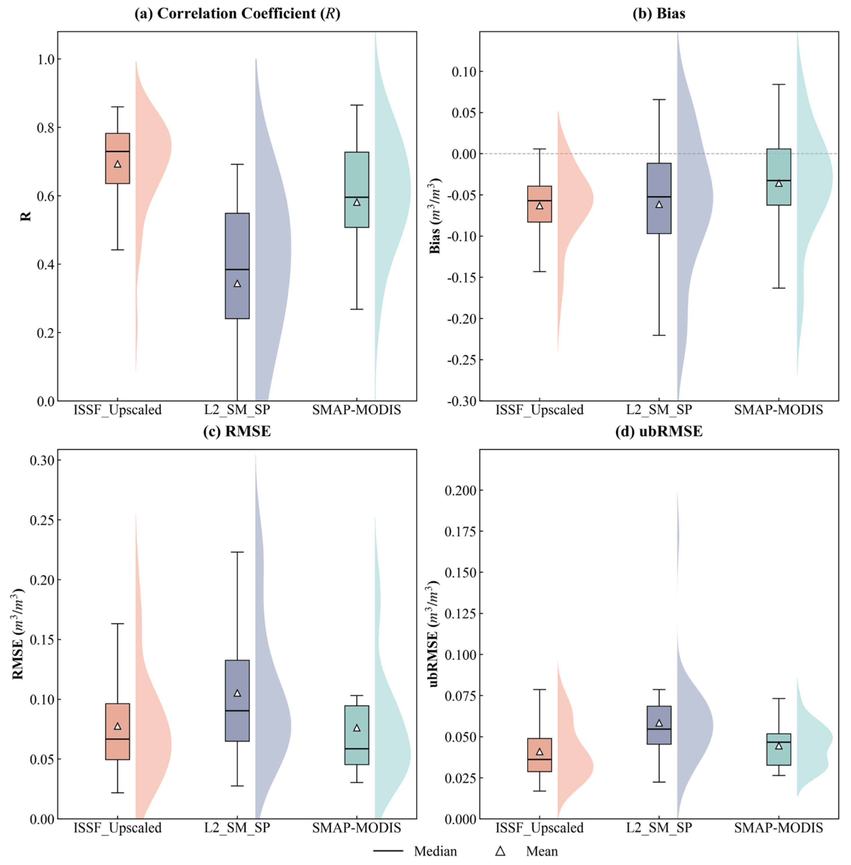
To place ISSF within existing SMAP-constrained high-resolution soil moisture products, ISSF was aggregated to 1 km and compared with L2_SM_SP and SMAP-MODIS at the station scale. This comparison was not intended to claim algorithmic superiority over these products, because they differ in retrieval philosophy, spatial support, and input data. Instead, it was used to examine whether ISSF produced reasonable station-scale behavior relative to existing SMAP-based products.
Figure 11 shows the station-level metric distributions for ISSF_Upscaled, L2_SM_SP, and SMAP-MODIS. In this comparison, ISSF_Upscaled showed a relatively concentrated metric distribution, with higher median temporal agreement and lower ubRMSE. L2_SM_SP showed a broader station-level distribution, while SMAP-MODIS showed an intermediate distribution.
All three SMAP-constrained products show a tendency toward negative bias. This common behavior suggests that part of the low-bias tendency in ISSF may be inherited from the SMAP-based moisture anchoring interval, rather than being caused only by the Sentinel-1 change-detection component. Such a systematic offset could in principle be reduced by an additional bias-correction step, although this would mainly improve the mean moisture level rather than the temporal agreement or unbiased error.

4.2.3. Regional Spatial Patterns and Texture Behavior

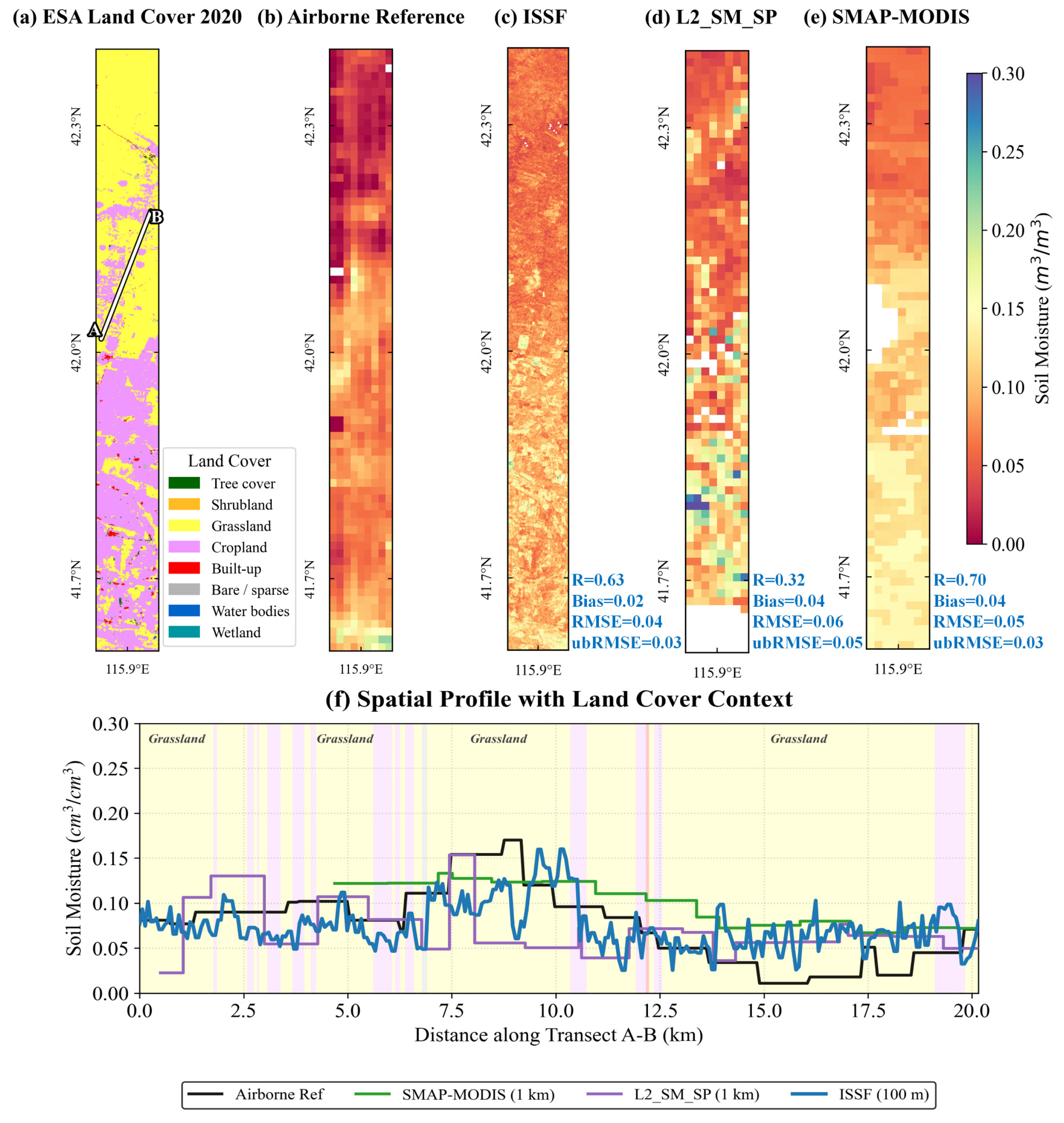
The regional spatial comparison further reveals differences among the three mapping routes (Figure 12). All three products reproduce the broad wet–dry gradient shown by the airborne reference, but they differ in local texture and spatial continuity. SMAP-MODIS captured the large-scale gradient clearly and showed a smoother spatial field. L2_SM_SP introduced finer-scale variations and stronger local contrasts for this event. ISSF preserved local wet–dry transitions while maintaining regional continuity across the cropland–grassland mosaic.
The transect along A–B shows the same pattern. The two 1 km products remain nearly constant over several kilometers, whereas ISSF retains more distinct local transitions within the same regional gradient. This behavior suggests that the Sentinel-1 change-detection component provides useful fine-scale texture, while the SMAP moisture anchoring helps maintain regional continuity.
The semivariogram was used as a supplementary regional texture diagnostic rather than as a standalone accuracy metric. The semivariogram comparison leads to a similar interpretation (Figure 13). ISSF follows a semivariogram trend that is closer to the airborne reference over the available scene. SMAP-MODIS shows a flatter curve, which is consistent with reduced high-frequency variability. L2_SM_SP shows stronger semivariance, suggesting a larger contribution from irregular local variation. These results indicate that ISSF reproduced the main wet–dry gradient and texture behavior for the available airborne event.

4.3. Direct-Transfer Stability in a Comparable Semi-Arid Region

To examine stability under direct transfer, the vegetation-conditioned parameterization calibrated in the Shandian River Basin was directly applied to the OzNet subset without local recalibration. OzNet in situ measurements were used as the reference. This test was designed to evaluate whether ISSF retained stable temporal behavior under comparable semi-arid cropland–grassland conditions, rather than to demonstrate broad geographic generalization.
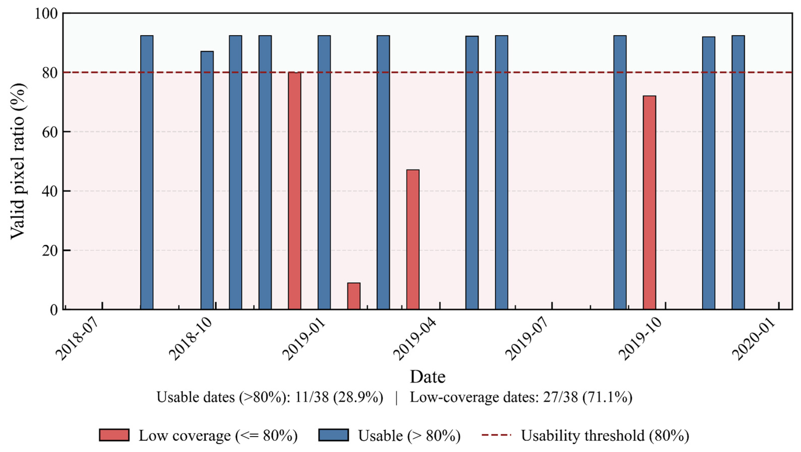
SMAP-MODIS was not included in this transfer test because its valid coverage over the OzNet study area was too limited during the study period. To quantify this limitation, the valid-pixel ratio of SMAP-MODIS was calculated for each evaluation date, as shown in Figure 14. Only 11 of the 38 dates had valid coverage above 80%, whereas the remaining 27 dates were affected by substantial missing data. Under this condition, including SMAP-MODIS in the OzNet time-series evaluation would have led to an uneven temporal comparison.
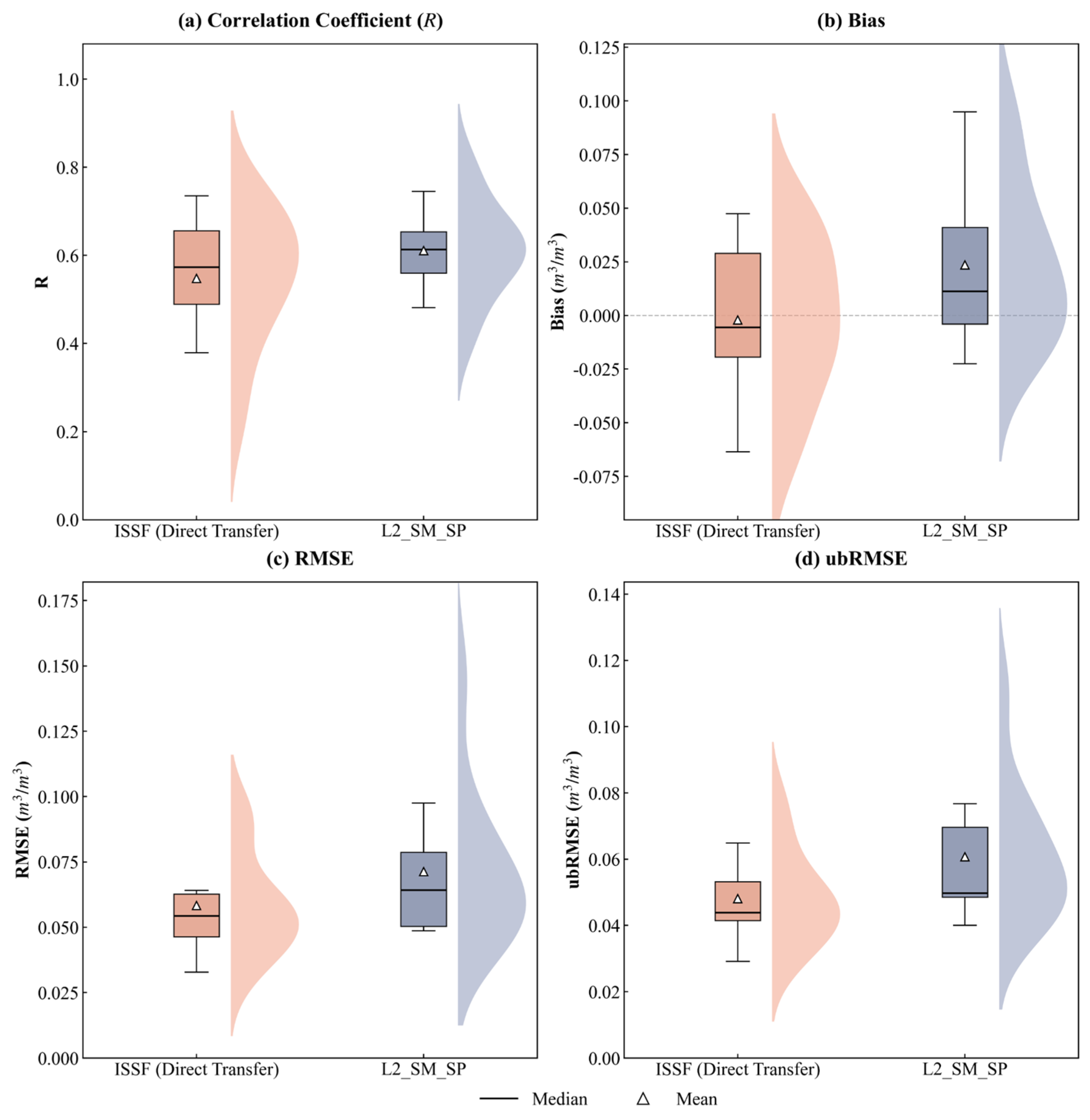
Figure 15 compares the station-level metric distributions of ISSF and L2_SM_SP under direct transfer. ISSF shows slightly lower correlation than L2_SM_SP, but its RMSE and ubRMSE distributions are more concentrated. The median ubRMSE of ISSF is about 0.04 m3 m−3, indicating relatively stable station-level temporal errors. In contrast, L2_SM_SP shows a more dispersed bias distribution and a wider high-error range, with a median ubRMSE of about 0.055 m3 m−3. These results indicate that the two products show different metric characteristics under direct transfer. ISSF showed a more concentrated error distribution across the selected OzNet sites, while L2_SM_SP showed slightly higher correlation.
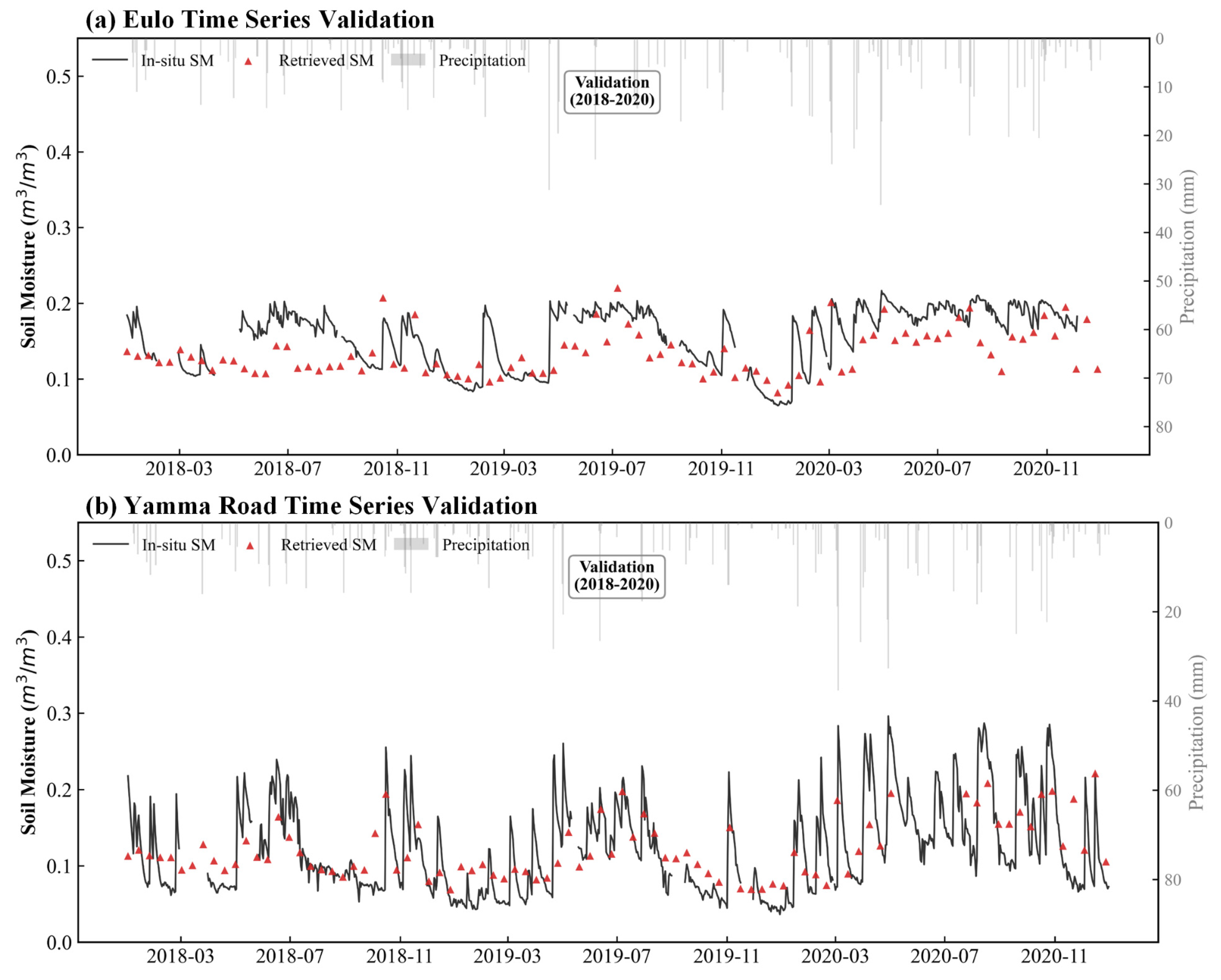
Figure 16 and Table 1 present time series at representative sites and accuracy statistics across all sites. Under direct transfer, ISSF captures the main wetting and drying cycles in the OzNet region. Across sites, ubRMSE remains below 0.05 m3/m3 for most stations. Compared with the modeling region, the cross-region evaluation shows a similar error level and no obvious change in the overall bias pattern.

4.4. Constraint Sensitivity Analysis

4.4.1. Sensitivity to Vegetation-Conditioned Upper-Bound Representation

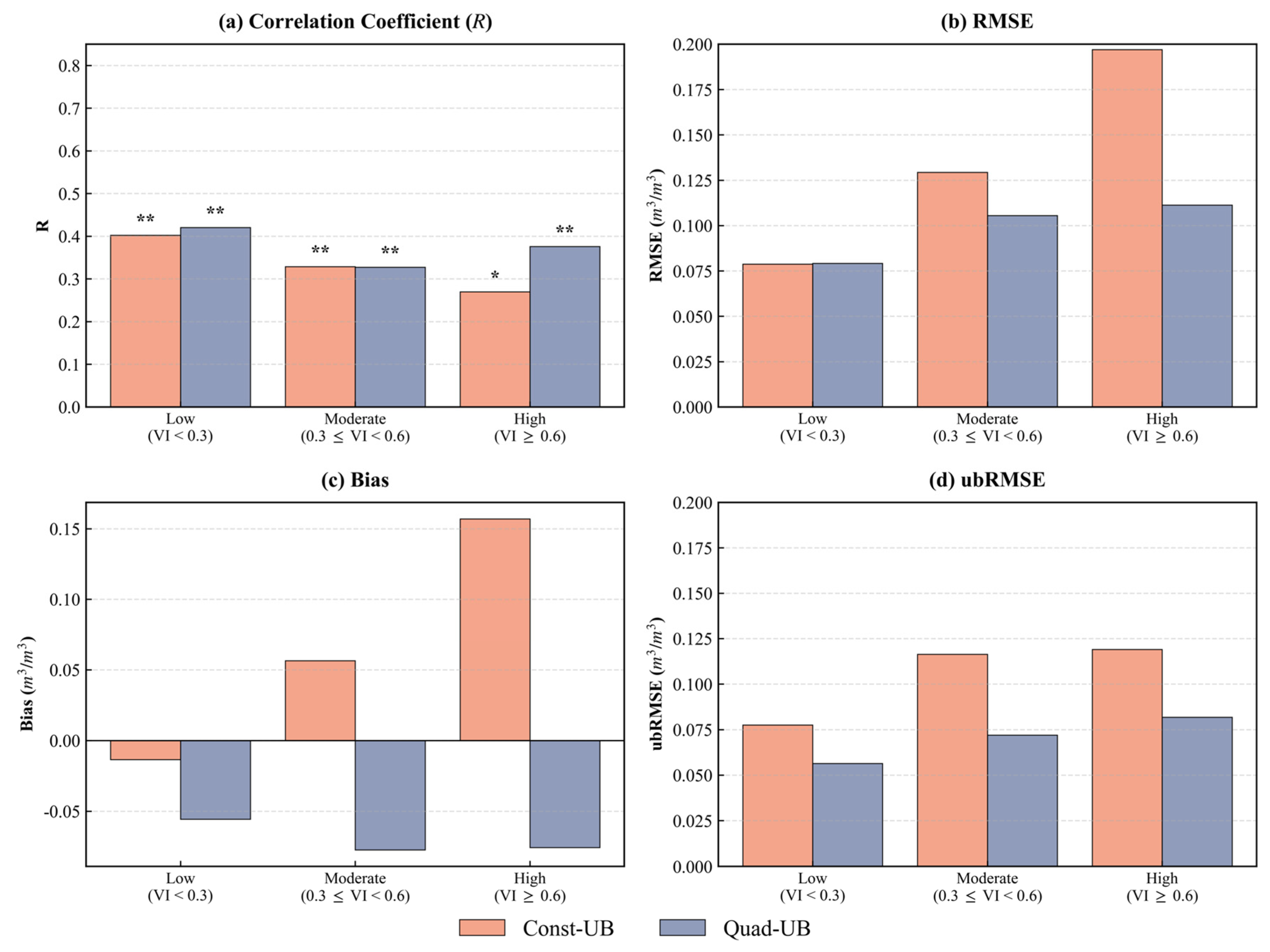
The sensitivity to the upper-bound representation was examined by comparing a fixed upper-bound scheme with the vegetation-conditioned quadratic scheme (Figure 17). Under low-vegetation conditions, the two schemes produced similar results. As vegetation increased, the advantage of the vegetation-conditioned scheme became more evident. In the moderate- and high-vegetation classes, the quadratic scheme reduced RMSE and ubRMSE and also reduced the bias relative to the fixed upper-bound scheme. This indicates that a single constant Δ σ max is insufficient when vegetation attenuation becomes stronger.
The linear and quadratic fits were further compared using the same bin-wise upper-bound samples (Figure 18). Both functions captured the decreasing tendency of Δ σ max with increasing NDVI, but the quadratic form better represented the curved upper-envelope behavior, especially over the middle and high NDVI ranges. Therefore, the quadratic NDVI-based upper-bound function was retained as the default vegetation-conditioned constraint in ISSF.
Additional tests on NDVI bin width and the number of top samples showed that the fitted upper-bound relation was stable within a reasonable parameter range. These results are provided in Table 2. The Top-N setting controls how the empirical upper envelope is extracted from each NDVI bin. A very small Top-N value can make the envelope sensitive to residual speckle noise, local geometric effects, or isolated mixed pixels. A much larger Top-N value may include more non-envelope observations and lower the estimated upper bound, which can reduce the effective backscatter-change dynamic range. The sensitivity analysis showed that Top-5 produced a lower R2 and a larger fitting RMSE than the default setting, whereas Top-10 and Top-15 produced similar fitting performance. This indicates that the fitted upper-bound relation was not strongly controlled by the exact Top-N choice around the default value. Therefore, Top-10 was retained as a practical default because it preserved the high-end backscatter-change signal while reducing dependence on individual extreme samples.

4.4.2. Sensitivity to Vegetation Information Source and Proxy Selection

Because the default ISSF uses NDVI as the vegetation proxy, two additional tests were conducted to evaluate the stability of the vegetation information used in the upper-bound model. First, the consistency between PROBA-V- and Landsat-derived NDVI was examined during the overlap period (Figure 19). The two NDVI series showed similar seasonal dynamics, and the downstream ISSF retrievals driven by the two NDVI sources were highly consistent. This suggests that the PROBA-V to Landsat transition introduced only limited uncertainty into the retrieval chain.
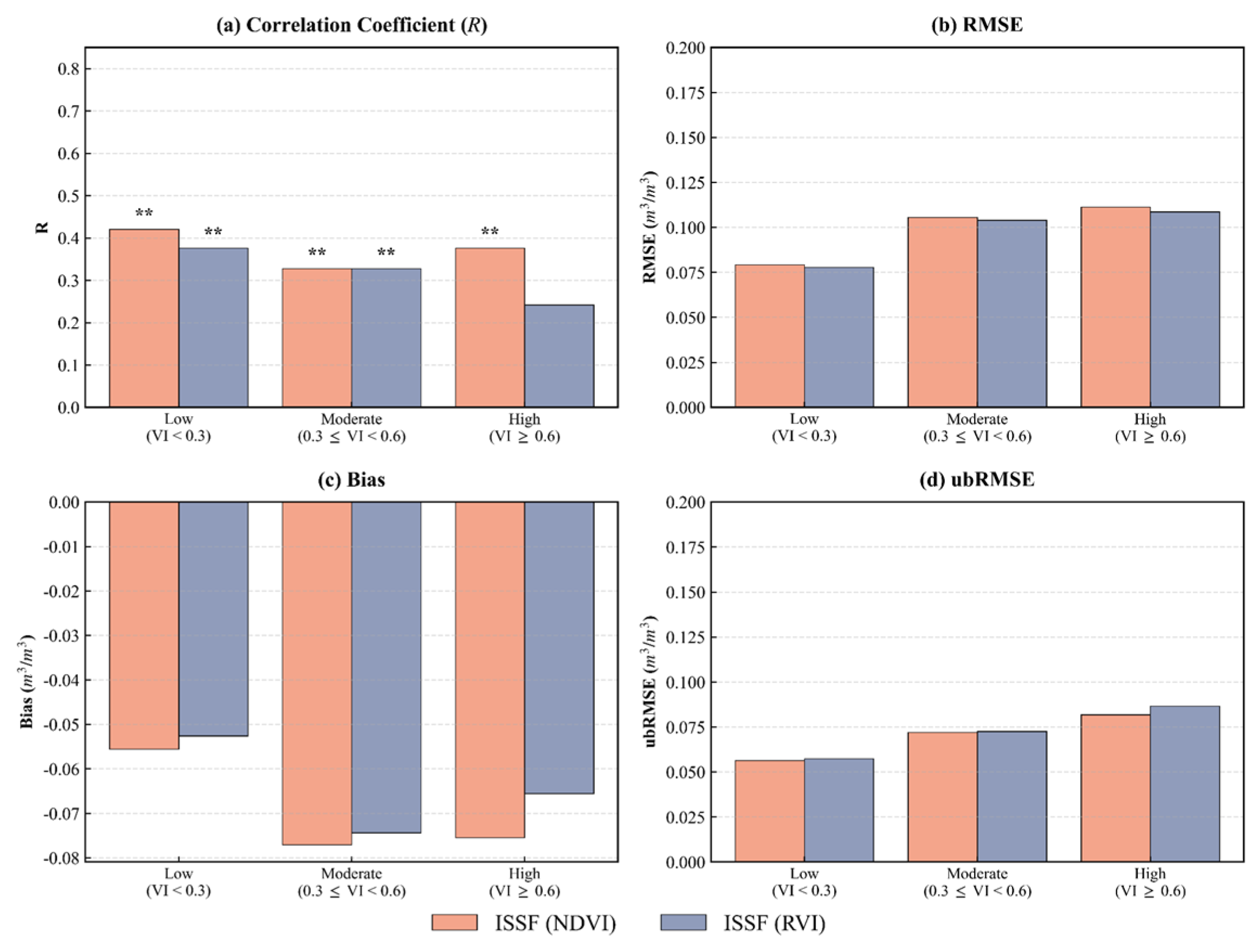
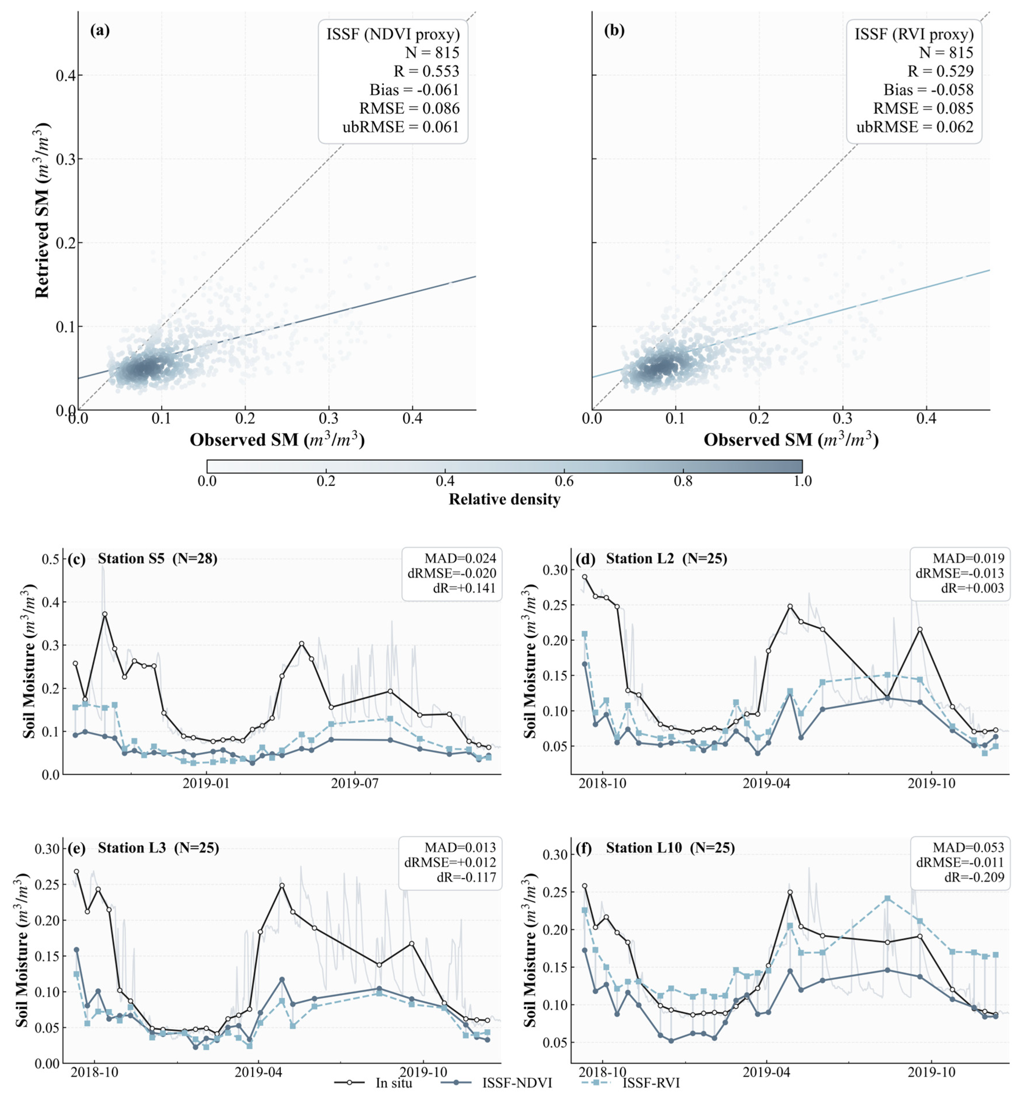
Second, RVI was tested as a radar-based alternative vegetation proxy (Figure 20 and Figure 21). Compared with the default NDVI-based implementation, ISSF(RVI) produced broadly similar retrieval patterns but did not provide a consistent improvement. Under low- and moderate-vegetation conditions, the differences between the two implementations were limited. Under high-vegetation conditions, RVI reduced the negative bias to some extent, but the correlation decreased and ubRMSE increased. These results indicate that the vegetation-conditioned framework is not restricted to optical vegetation information, but NDVI remains the more stable default proxy. RVI should be interpreted as a feasible alternative when optical observations are unavailable or unstable, rather than as a replacement for the default NDVI-based implementation.

4.4.3. Effects of SMAP-Based Moisture Anchoring and Boundary Scale

The full-record 1st/99th percentile setting was retained because it provided stable results across tested temporal windows and quantile settings, while reducing the influence of short-term extremes (Appendix A).
The SMAP-based moisture anchoring provides the volumetric reference for scaling Sentinel-1-derived relative wetness. However, because the default dry/wet anchors are defined at the original SMAP 9 km scale, they may constrain the expression of sub-grid soil moisture variability. The VRR analysis (Figure 22) shows that ISSF retained part of the within-cell spatial dispersion observed in the airborne reference, but the retained variability differed among SMAP grid cells. This indicates that SMAP anchoring does not remove all Sentinel-1-derived local variability, but it compresses part of the sub-grid wet–dry contrast.
To examine whether a finer-scale passive-microwave anchoring interval could reduce this constraint, DSCALE_MOD16-downscaled SMAP soil moisture was used to generate alternative dry/wet anchors (Figure 23b,c). However, this finer-scale boundary information did not reduce the high-wet station-sample error, with ubRMSE remaining nearly unchanged between ISSF-SMAP and ISSF-DSCALE (Figure 23d). In contrast, the airborne event comparison showed a slight improvement in area-scale agreement when DSCALE_MOD16 anchoring was used. The correlation increased from 0.633 to 0.651, RMSE decreased from 0.037 to 0.033 m3 m−3, and ubRMSE remained 0.028 m3 m−3 (Figure 23i,j). These results indicate that DSCALE_MOD16 anchoring can enhance local spatial texture and slightly improve event-scale spatial consistency, but it does not provide a consistent improvement in station-level wet-end error. Therefore, the original SMAP 9 km anchoring interval was retained as the default ISSF configuration, while DSCALE_MOD16 was used as a boundary-scale sensitivity test.

5. Discussion

5.1. Vegetation Controls on Backscatter-Change Sensitivity

The vegetation-stratified results show that ISSF performance degraded as vegetation cover increased, but this degradation did not indicate a complete loss of the Sentinel-1 temporal signal. The key question is why vegetation mainly weakened the reliability of volumetric soil moisture retrieval while part of the wet–dry temporal variation was still retained. A plausible explanation is that vegetation changes the transfer relationship between soil-moisture variation and C-band backscatter response. Under the water cloud model, the observed C-band backscatter over vegetated surfaces can be decomposed into vegetation volume scattering and soil scattering attenuated by the canopy [47,56]. Recent Sentinel-1 soil moisture studies have also identified vegetation attenuation, vegetation structure, and time-varying surface conditions as major limitations for C-band retrieval [57,58]. Therefore, the same soil-moisture change may produce a smaller observable VV backscatter-change amplitude under higher vegetation cover. In this study, the NDVI-dependent upper envelope indicates that the fitted observable VV backscatter-change range varied with vegetation condition. This pattern is consistent with a vegetation-induced narrowing of the usable change range. The vegetation-stratified validation further shows that this narrowing coincided with degraded retrieval accuracy under higher vegetation cover.
This amplitude-compression mechanism explains the role of the vegetation-conditioned upper bound in ISSF. In the retrieval equation, the Sentinel-1-derived relative wetness is controlled by the ratio between the observed backscatter change and the maximum observable backscatter-change range. If a fixed upper bound is used, the same Δσ value is normalized against the same dynamic range under both sparse and more vegetated conditions. This assumption becomes problematic when vegetation attenuation reduces the maximum observable soil-moisture-related response. In that case, the fixed upper bound can underestimate relative wetness, especially under wet or more vegetated conditions. The NDVI-conditioned upper bound reduces this mismatch by assigning a vegetation-specific dynamic range before SMAP-based volumetric scaling. Therefore, its benefit is limited when canopy attenuation is weak, but becomes clearer when vegetation effects are stronger. This improvement should be interpreted as a dynamic-range normalization within the retrieval equation, rather than as a post-retrieval bias correction.
The quadratic NDVI-based function should be interpreted as an empirical upper-envelope approximation of the vegetation-dependent observable dynamic range. It is physically motivated by vegetation attenuation, but it is not a full vegetation scattering model. The function was calibrated from the observed relationship between NDVI and the maximum detectable Sentinel-1 VV backscatter-change range in the study area. Therefore, its use should be limited to vegetation conditions comparable to those sampled in this study. The RVI-based test further indicates that the proposed upper-bound framework is not tied to optical vegetation information only. However, RVI did not provide a consistent improvement in the present experiments, so NDVI was retained as the default proxy. This result suggests that alternative vegetation indicators may be useful when optical observations are unavailable or unstable, but their use should be evaluated before transfer to new regions.
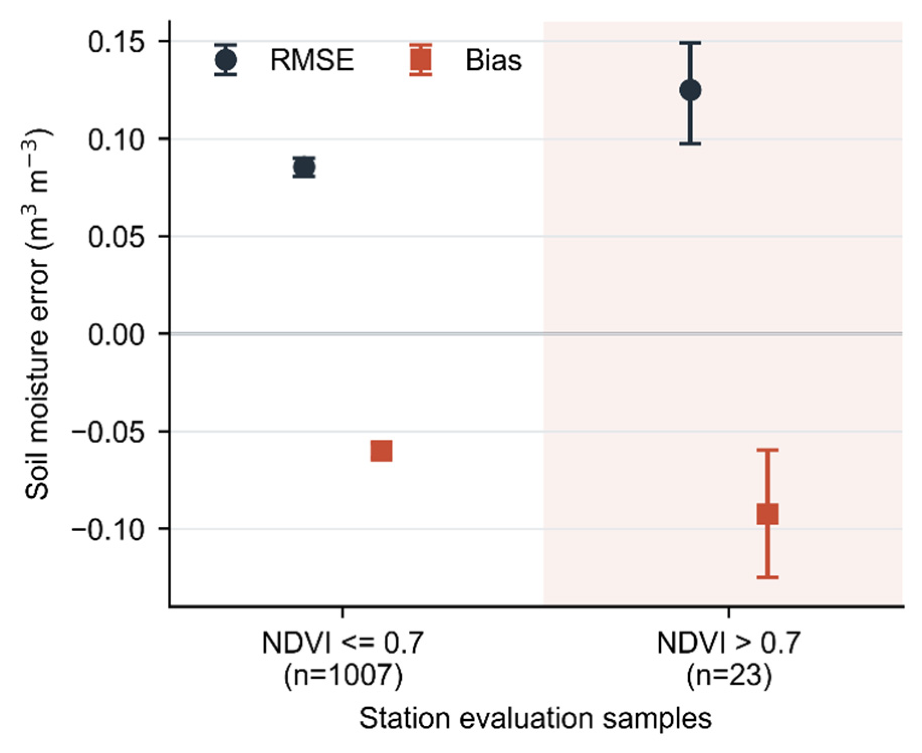
A diagnostic comparison was further conducted for saturation-prone high-NDVI samples. Samples with NDVI > 0.7 accounted for only 23 of 1030 station samples (2.2%) and 2.4% of all valid pixel–date pairs, indicating that the overall evaluation was not dominated by this range. However, the NDVI > 0.7 samples showed higher RMSE and stronger negative bias than the NDVI ≤ 0.7 samples (Figure 24). Because the number of high-NDVI station samples was small, this result should be interpreted as a diagnostic indication of increased uncertainty rather than as a robust independent stratified validation. This supports treating NDVI > 0.7 as a caution zone for volumetric ISSF retrieval.

5.2. Scale-Dependent Moisture Anchoring and Wet-End Bias

SMAP anchoring stabilizes the conversion from Sentinel-1-derived relative wetness to volumetric soil moisture, but its coarse spatial support can limit the fine-scale wet–dry contrast retained in ISSF. Passive microwave observations provide the volumetric reference, whereas Sentinel-1 contributes finer-scale change information [59,60]. Accordingly, the multi-year SMAP quantiles should be interpreted as empirically stable moisture bounds rather than strict physical limits. The VRR analysis showed that ISSF retained part of the within-cell variability, while some sub-grid contrast was compressed by the 9 km anchoring interval.
This scale mismatch provides a plausible explanation for the observed wet-end underestimation. Local wet peaks at 100 m are scaled using dry and wet bounds shared within a coarse SMAP grid cell, which can damp spatially localized moisture extremes. Reduced C-band soil sensitivity under wet or vegetated conditions may further strengthen this effect [58]. The combined influence of coarse wet-boundary smoothing and weaker soil contributions therefore appears mainly as negative volumetric bias at the wet end.
Increasing the spatial detail of the moisture anchors did not consistently remove this limitation. DSCALE_MOD16 anchoring slightly improved the airborne event-scale agreement but did not reduce the high-wet station-sample error. This contrast indicates that finer downscaled spatial texture does not necessarily provide more accurate local dry and wet bounds. Spatial detail introduced by auxiliary downscaling variables may improve the mapped texture without correcting the absolute moisture scale. The original SMAP anchoring was therefore retained as the default configuration.
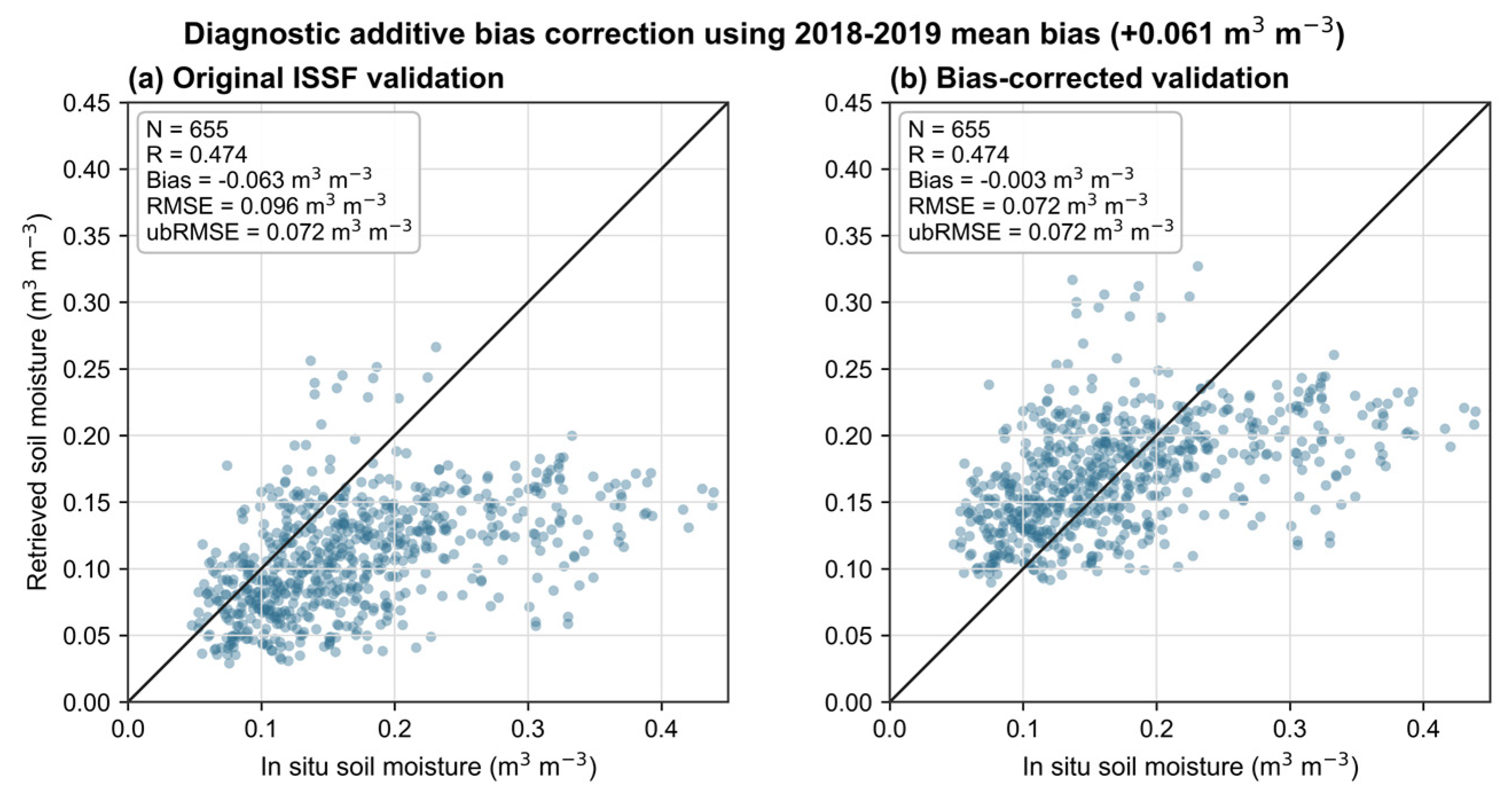
The residual systematic offset was further examined through a diagnostic additive bias-correction test for the independent 2020–2021 validation period. The mean bias estimated from the 2018–2019 modeling period was −0.061 m3 m−3; its opposite value, +0.061 m3 m−3, was applied unchanged to all 655 independent validation samples. Bias decreased from −0.063 to −0.003 m3 m−3, and RMSE decreased from 0.096 to 0.072 m3 m−3 (Figure 25). In contrast, R and ubRMSE remained unchanged at 0.474 and 0.072 m3 m−3, respectively. This behavior is expected because adding a constant shifts the mean retrieval level without changing temporal covariation or centered errors. Additive correction can therefore reduce regional mean offset, but it does not improve the underlying retrieval dynamics. Because it also requires representative regional reference data, it was not included as a default ISSF component and should instead be considered an optional regional post-processing step.
The current evaluation also has a resolution-related uncertainty boundary. Although ISSF produces 100 m retrievals, the independent in situ observations are point measurements and cannot fully represent the spatial mean of a 100 m pixel. The neighborhood-scale analysis was therefore used to diagnose point-to-pixel representativeness effects, rather than to provide a complete native-pixel validation. In addition, the airborne and product comparisons required aggregation to 1 km or coarser scales. These comparisons are useful for evaluating regional wet–dry gradients and spatial texture, but spatial aggregation can also reduce random pixel-scale errors. Therefore, the current results support the temporal consistency and event-scale spatial behavior of ISSF, while true 100 m pixel-level accuracy still requires dense ground sampling or higher-resolution independent reference data.

5.3. Transferability Under Land-Cover and Surface-Condition Constraints

The OzNet experiment provides a direct-transfer assessment under conditions that are broadly comparable to the modeling region. The vegetation-conditioned parameterization calibrated in the Shandian River Basin was applied to OzNet without local recalibration, which allowed us to examine whether the parameterization remained stable in another semi-arid cropland-grassland region. However, this test does not cover the full range of climate, vegetation, and management conditions that would be required to demonstrate general transferability. Similar concerns have been noted for Sentinel-1 soil moisture retrieval, where regional calibration and evaluation under different environmental contexts remain important for improving robustness [58]. The OzNet results therefore indicate transfer stability within a similar semi-arid and open-canopy setting. Broader transferability across contrasting environmental regimes still requires additional evaluation.
Performance is expected to be more limited when ISSF is applied to humid agricultural systems or forested environments. In humid croplands, Sentinel-1 soil moisture retrieval can be strongly affected by vegetation development, soil wetness, and C-band penetration-depth variability during crop cycles [57]. More frequent rainfall or irrigation, denser seasonal canopy development, and possible surface water or canopy-interception effects may therefore weaken the direct relationship between Sentinel-1 backscatter and near-surface soil moisture. In forested environments, dense vegetation, vegetation structure, and surface roughness are persistent uncertainty sources for Sentinel-1 soil moisture retrieval [58]. The soil contribution to C-band backscatter may be further reduced by canopy attenuation and structural scattering. These conditions were not represented in the present transfer experiment. Therefore, the performance of ISSF in humid agricultural regions or forests remains an extrapolation beyond the current validation domain and requires dedicated evaluation before operational use.
Seasonal agricultural management is another factor that can affect transferability. Sentinel-1 change-detection retrieval assumes that non-moisture scattering controls, including vegetation structure and surface roughness, vary more slowly than soil moisture over the reference period. This assumption underlies short-term change-detection approaches, which rely on surface parameters that do not change substantially relative to soil moisture [28,61]. It may be weakened after tillage, harvesting, residue exposure, or other management operations, because these processes can modify VV and VH backscatter independently of soil moisture. Field-scale Sentinel-1 studies have reported that tillage and harvesting can cause abrupt roughness changes and non-negligible variations in total backscatter [62].
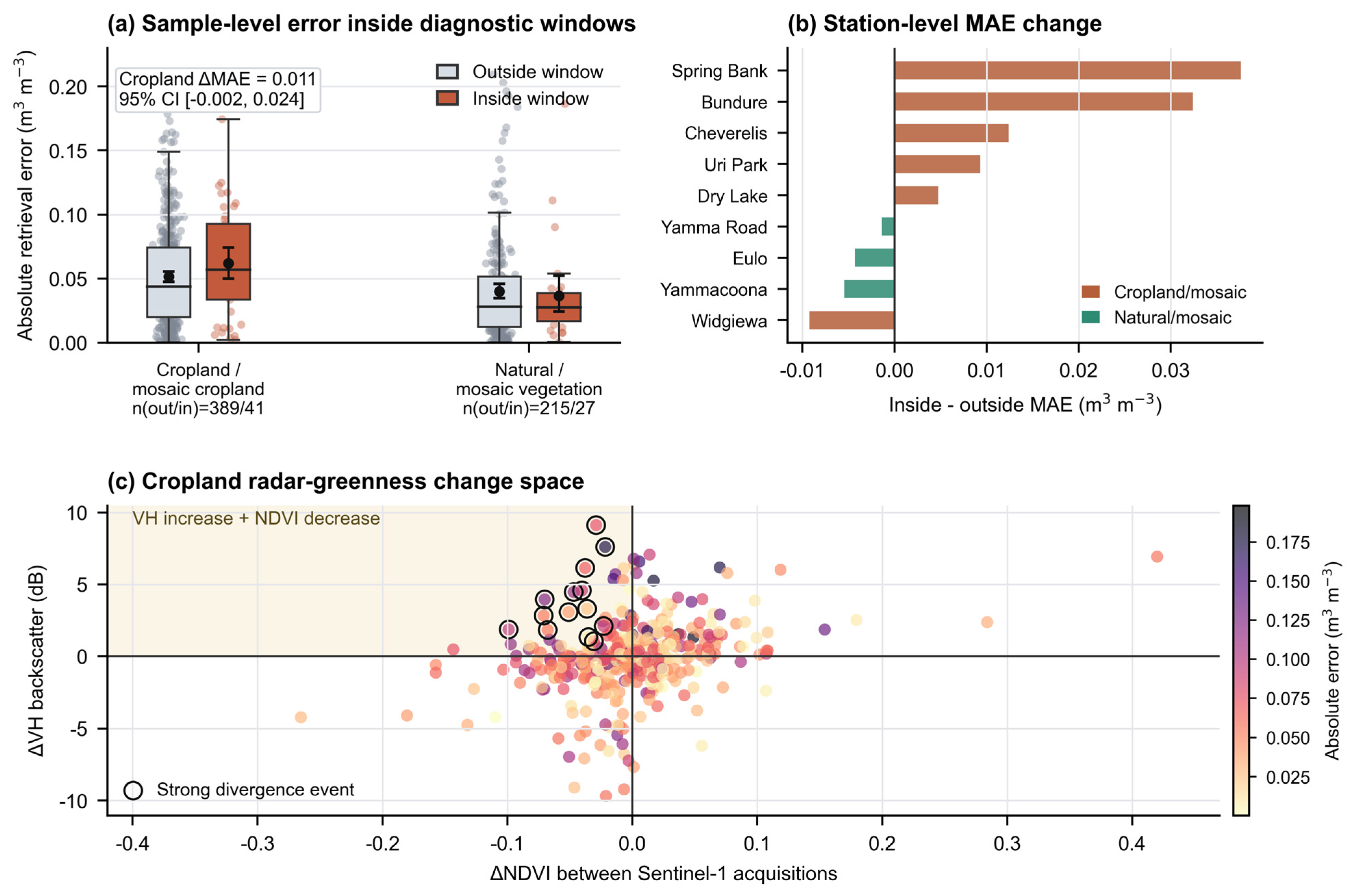
We used the VH-NDVI divergence diagnostic to examine whether lower transfer stability at some OzNet cropland sites was associated with non-moisture scattering changes (Figure 26). The diagnostic flagged periods when VH backscatter increased while NDVI decreased, a pattern that may indicate changes in crop structure, residue exposure, or surface roughness rather than soil moisture alone [62,63]. Validation samples within ±12 days of these divergence events were then compared with samples outside the windows. In cropland and mosaic-cropland sites, MAE increased from 0.051 to 0.062 m3 m−3 near divergence events, with detectable differences at both the sample level (p = 0.042) and station level (p = 0.047). Natural and mosaic-natural vegetation sites did not show the same error increase. These results suggest that non-moisture scattering changes partly contributed to the weaker transfer stability observed at some agricultural sites.
Overall, the OzNet experiment should be viewed as a useful but limited direct-transfer test. It suggests that ISSF can retain stable performance when applied to a comparable semi-arid cropland-grassland region without local recalibration. At the same time, the results indicate that transferability is constrained by vegetation density, hydroclimatic regime, and management-induced surface changes. Future applications should therefore include additional validation in humid agricultural systems, forested regions, and management-intensive croplands, together with disturbance screening or roughness-sensitive indicators.

5.4. Large-Area Applicability and Methodological Positioning

The potential use of ISSF over larger areas depends on both computational feasibility and the stability of its input assumptions. From the computational perspective, ISSF has the potential for large-area implementation because the core retrieval is pixel-wise and does not require local model training. After Sentinel-1, NDVI, and SMAP inputs are prepared, each valid pixel–date only requires backscatter-change calculation, NDVI-conditioned upper-bound evaluation, relative wetness normalization, and SMAP dry/wet-anchor scaling. The computational cost is therefore expected to increase approximately linearly with the number of valid pixel–date observations. In large-area applications, the main processing burden would come from Sentinel-1 preprocessing, time-series compositing, temporal matching with NDVI and SMAP, and tile-based raster input/output, rather than from the retrieval equation itself.
This large-area use also depends on whether the target region remains within the assumptions tested in this study. As discussed above, dense vegetation, wet conditions, and management-induced roughness changes can weaken the Sentinel-1 soil-moisture signal or violate the stable-surface assumption. Therefore, continental-scale application would require appropriate masking, quality control, or disturbance screening before interpreting the retrievals as volumetric soil moisture. In this sense, ISSF is computationally scalable, but its physical applicability should still be constrained by vegetation, hydroclimatic, and land-management conditions.
Recent CNN, LSTM, and other learning-based retrieval frameworks provide powerful tools for high-resolution soil moisture estimation because they can integrate Sentinel-1, Sentinel-2, passive microwave, terrain, soil, and meteorological information and learn nonlinear spatial-temporal relationships from representative training datasets [18,64]. ISSF follows a different route. It is not intended to replace learning-based approaches, but provides a low-training-dependence and explicitly constrained framework for 100 m soil moisture mapping. Its retrieval pathway links Sentinel-1 backscatter change, NDVI-conditioned dynamic-range constraint, and SMAP dry/wet anchoring, which makes the main assumptions and uncertainty sources easier to examine. Therefore, ISSF and learning-based methods are complementary. The constraints used in ISSF may also provide useful prior information for future hybrid or physically informed machine learning frameworks.

6. Conclusions

This study proposed ISSF, an improved SMAP-anchored Sentinel-1 change-detection framework, for 100 m surface soil moisture mapping. ISSF improves the conventional Sentinel-1 change-detection method by introducing two constraints. First, a vegetation-conditioned upper-bound function was used to describe the reduction in the observable backscatter-change range under different vegetation conditions. Second, multi-year SMAP dry/wet anchoring intervals were used to convert Sentinel-1-derived relative wetness into volumetric soil moisture. In this framework, Sentinel-1 provides fine-scale temporal change information, while SMAP provides a coarse-scale volumetric moisture reference.
ISSF was evaluated using in situ soil moisture measurements, a near-concurrent airborne reference, SMAP-based regional products, and a stability test under direct transfer to OzNet. In the Shandian River Basin, ISSF achieved a point-scale performance of R = 0.549 and ubRMSE = 0.062 m3 m−3. Relative to three benchmark change-detection methods, ISSF increased R by 11–53% and reduced ubRMSE by 7–15%. For the available airborne-referenced event, ISSF showed area-scale agreement with R = 0.635 and ubRMSE = 0.027 m3 m−3, and the semivariogram comparison indicated a regional texture trend broadly consistent with the airborne reference. Under direct transfer to OzNet without local recalibration, ISSF achieved a mean R of 0.55 and a mean ubRMSE of 0.05 m3 m−3. These results suggest that ISSF can provide stable 100 m soil moisture estimates under sparse to moderate-vegetation conditions and comparable semi-arid cropland–grassland environments.
The sensitivity analyses further clarified the role and limitation of the two constraints. The vegetation-conditioned upper-bound representation improved the normalization of Sentinel-1 backscatter changes when vegetation attenuation became stronger. NDVI remained the default vegetation proxy, while RVI provided a feasible radar-based alternative when optical vegetation observations were unavailable or unstable. The SMAP-based moisture anchoring was stable across reasonable temporal windows and quantile settings, but it also constrained part of the sub-grid soil moisture variability. The DSCALE_MOD16-based boundary test introduced finer spatial texture and slightly improved the airborne event-scale comparison, but it did not reduce station-level wet-end errors. Therefore, the original SMAP 9 km anchoring interval was retained as the default configuration.
Several limitations remain. ISSF still shows reduced skill under dense vegetation, very wet soil conditions, and disturbed cropland surfaces. Dense vegetation weakens C-band sensitivity to soil moisture, high-moisture conditions are associated with systematic underestimation, and tillage or residue changes can introduce non-moisture backscatter variations. Therefore, ISSF should be interpreted as a constrained recovery of fine-scale soil moisture variability rather than a lossless reconstruction of the full 100 m dynamic range. Further evaluation is still needed before extending the framework to humid, tropical, or densely vegetated regions. Future work should improve vegetation characterization under cloudy or rapidly changing conditions, account for surface roughness and crop-residue disturbances, and extend evaluation across more contrasting climate, vegetation, and land-management settings.

Author Contributions

Y.W. (Yunjia Wang): Validation, Formal analysis, Software, Visualization, Investigation, Writing—Original draft preparation; H.S.: Writing—review & editing, Writing—original draft, Supervision, Resources, Project administration, Methodology, Funding acquisition, Conceptualization; H.P.: Investigation, Software, Review & editing; J.G.: Investigation, Software, Review & editing; Z.X.: Investigation, Software, Review & editing; Y.W. (Yuxin Wang): Investigation, Software; D.W.: Investigation, Software. All authors have read and agreed to the published version of the manuscript.

Funding

This research was supported by Beijing Natural Science Foundation (grant number L251050), National Natural Science Foundation of China (grant number 42471381), National Key R&D Program of China (grant number 2024YFC2607703-5), supported by the Ph.D. Top Innovative Talents Fund of CUMTB, BBJ2026046, and China Fundamental Research Funds for Central Universities (Grant numbers: 2026JCCXDC05).

Data Availability Statement

The Sentinel-1 GRD data used in this study are freely available. The SMAP Enhanced L3 Radiometer Global and Polar Grid Daily 9 km EASE-Grid Soil Moisture, Version 6 is from the NSIDC DAAC (https://doi.org/10.5067/M20OXIZHY3RJ) [65]. The PROBA-V Level-3 TOC-NDVI data are from the PROBA-V data portal (https://doi.org/10.5270/PRV-htrh1c8) [66]. The SMAP/Sentinel-1 L2 Radiometer/Radar 30-Second Scene 3 km EASE-Grid Soil Moisture, Version 3 is from the NSIDC DAAC (https://doi.org/10.5067/ASB0EQO2LYJV) [29]. The SMAP-Derived 1-km Downscaled Surface Soil Moisture Product, Version 1 is from the NSIDC DAAC (https://doi.org/10.5067/U8QZ2AXE5V7B) [41]. The in situ soil moisture observations are from the International Soil Moisture Network (https://doi.org/10.5194/hess-15-1675-2011) [67], the OzNet soil moisture monitoring network (https://doi.org/10.1029/2012WR011976) [37], and the Luan River network used for the Shandian River Basin evaluation in this study (https://doi.org/10.1016/j.rse.2020.111680) [35]. The Shandian River Basin soil moisture retrieval results generated in this study are available in Zenodo at https://doi.org/10.5281/zenodo.19362893 [68].

Acknowledgments

The author would like to thank the International Soil Moisture Network (ISMN) team for providing and maintaining high-quality global soil moisture observations. We also acknowledge Google Earth Engine (GEE) platform for data access and the following data providers: NASA SMAP mission, the European Space Agency (ESA) and the Copernicus Programme for providing Sentinel-1 SAR products, and the PROBA-V mission team for the PROBA-V C1 Top-of-Canopy NDVI product.

Conflicts of Interest

The authors declare no conflicts of interest.

Appendix A

To examine the robustness of the SMAP boundary anchoring scheme, two sensitivity analyses were conducted. The first evaluated the effect of the temporal length used to define the SMAP dry-wet bounds. The second evaluated the effect of different quantile settings used for boundary estimation.
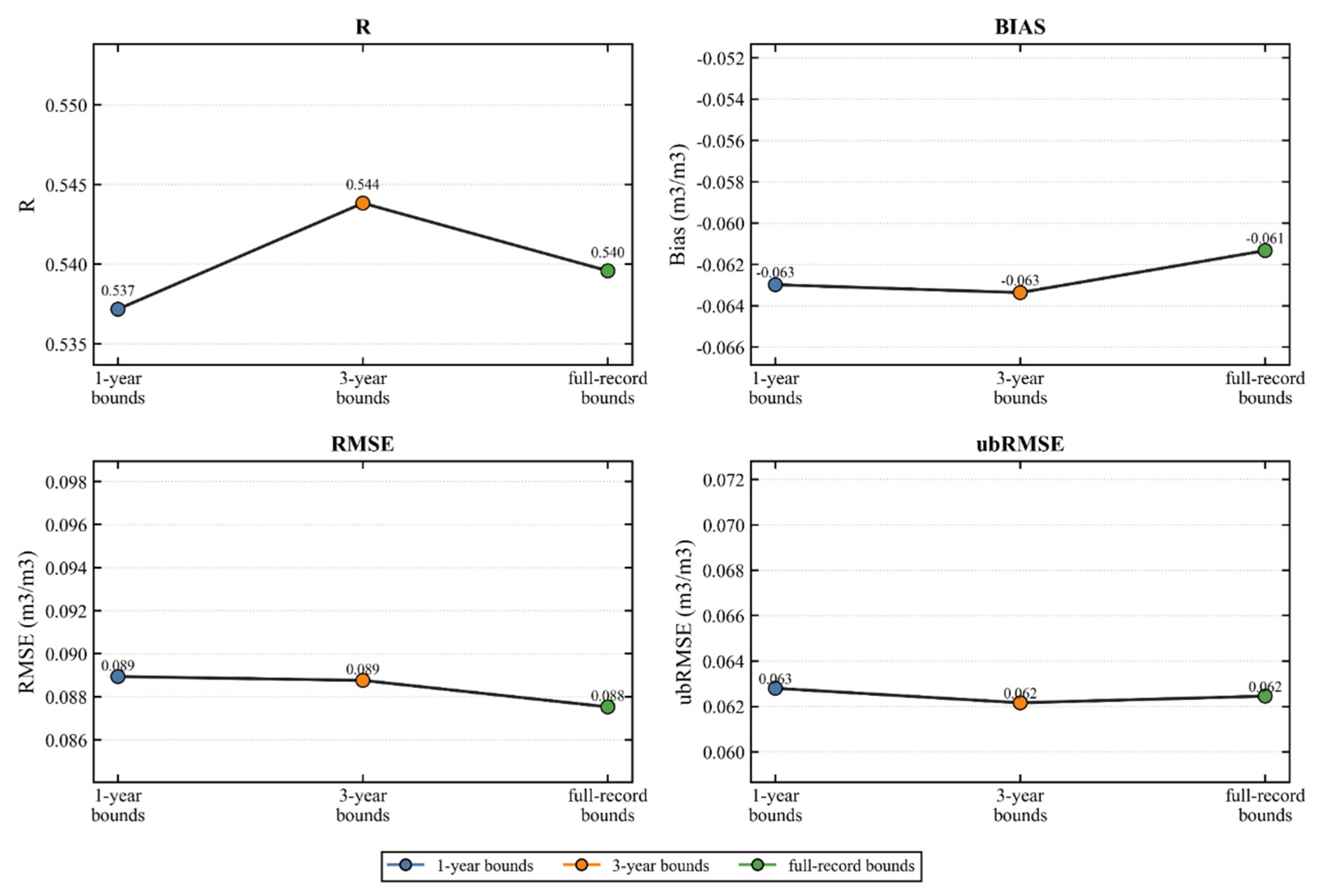
As shown in Figure A1, the retrieval results were similar under the 1-year, 3-year, and full-record boundary settings. The 3-year bounds gave the highest correlation (R = 0.544), whereas the full-record bounds gave a slightly lower RMSE (0.088 m3/m3) and a smaller bias (−0.061 m3/m3), with the same ubRMSE (0.062 m3/m3) as the 3-year bounds. The 1-year bounds produced slightly weaker overall performance. These results indicate that the retrieval is not highly sensitive to the temporal length of the SMAP reference period within the tested range. The full-record setting was retained in the final implementation because it uses the longest available SMAP record and provides a more stable reference for interannual hydroclimatic variability while maintaining comparable retrieval accuracy.
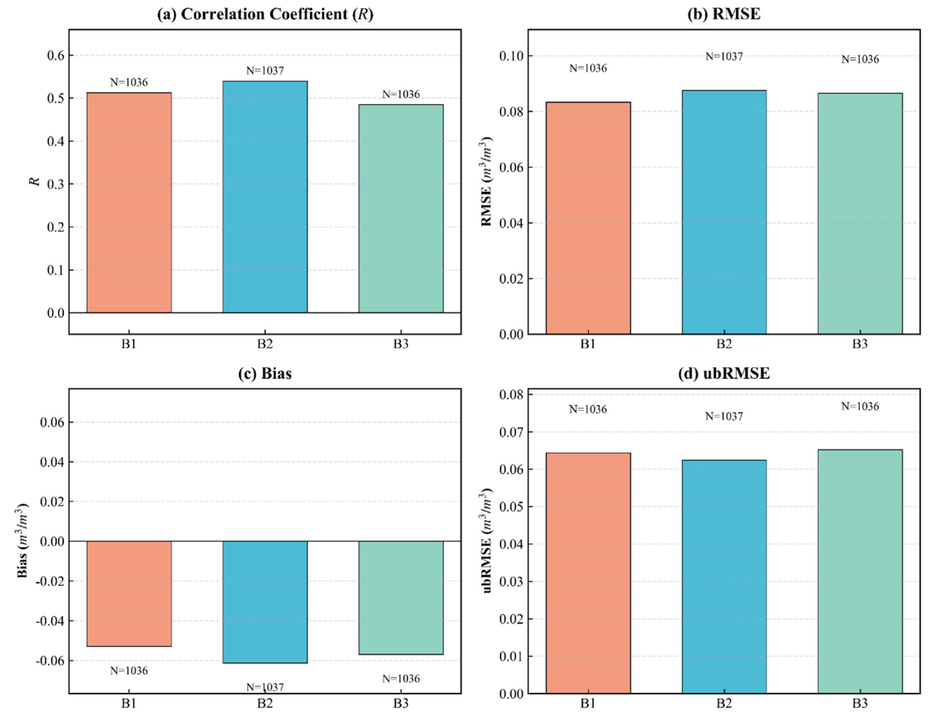
The sensitivity to the quantile definition is shown in Figure A2, where three boundary settings were compared: B1 (q0/q100), B2 (q1/q99), and B3 (q5/q95). The three settings produced broadly comparable results, but some differences were observed. B2 gave the highest correlation and the lowest ubRMSE, indicating a better representation of temporal variability. B1 gave a slightly lower RMSE and a smaller bias, but it relies on absolute minimum and maximum values and is therefore more sensitive to outliers. B3 further narrowed the dry-wet interval, which weakened the dynamic range available for retrieval and reduced correlation. Based on these results, the 1/99 quantile setting was retained as the default configuration because it provides a balanced compromise between robustness to outliers and preservation of the effective retrieval range.
To further examine the potential influence of frozen-season sampling on SMAP boundary estimation, monthly availability statistics of valid SMAP observations were compiled for the Shandian River Basin. As shown in Figure A3, almost no valid SMAP data are available in January, February, late November, and December. In contrast, most valid observations occur from April to October. This distribution indicates that the dry-wet boundary calculation was dominated by non-frozen or transitional periods rather than by deep-winter frozen conditions. It therefore supports the interpretation that frozen-season SMAP samples had only limited influence on the estimation of M v dry and M v wet in this study.
Figure A1. Sensitivity of ISSF retrieval performance to the temporal length of SMAP dry–wet bounds. Station-level validation metrics, including R, Bias, RMSE, and ubRMSE, are compared for retrievals using 1-year (2015), 3-year (2015–2017), and full-record (2015–2022) SMAP boundary settings.
Remotesensing 18 02045 g0a1
Figure A2. Sensitivity of ISSF retrieval performance to different SMAP boundary quantile settings.
Remotesensing 18 02045 g0a2
Figure A3. Monthly number of valid SMAP days in the Shandian River Basin during the study period. Bars denote the number of valid SMAP observations in each month, and labels show the monthly count and valid rate.
Remotesensing 18 02045 g0a3

References

  1. Demargne, J.; Wu, L.M.; Regonda, S.K.; Brown, J.D.; Lee, H.; He, M.X.; Seo, D.J.; Hartman, R.; Herr, H.D.; Fresch, M.; et al. The Science of NOAA’s Operational Hydrologic Ensemble Forecast Service. Bull. Am. Meteorol. Soc. 2014, 95, 79–98. [Google Scholar] [CrossRef]
  2. Green, J.K.; Seneviratne, S.I.; Berg, A.M.; Findell, K.L.; Hagemann, S.; Lawrence, D.M.; Gentine, P. Large Influence of Soil Moisture on Long-Term Terrestrial Carbon Uptake. Nature 2019, 565, 476–479. [Google Scholar] [CrossRef] [PubMed]
  3. Xu, Z.H.; Sun, H.; Zhang, T.; Xu, H.Y.; Wu, D.; Gao, J.H. Evaluating established deep learning methods in constructing integrated remote sensing drought index: A case study in China. Agric. Water Manag. 2023, 286, 108405. [Google Scholar] [CrossRef]
  4. Kornelsen, K.C.; Coulibaly, P. Advances in soil moisture retrieval from synthetic aperture radar and hydrological applications. J. Hydrol. 2013, 476, 460–489. [Google Scholar] [CrossRef]
  5. Zhao, T.; Hu, L.; Shi, J.; Lü, H.; Li, S.; Fan, D.; Wang, P.; Geng, D.; Kang, C.S.; Zhang, Z. Soil moisture retrievals using L-band radiometry from variable angular ground-based and airborne observations. Remote Sens. Environ. 2020, 248, 111958. [Google Scholar] [CrossRef]
  6. Entekhabi, D.; Njoku, E.G.; O’Neill, P.E.; Kellogg, K.H.; Crow, W.T.; Edelstein, W.N.; Entin, J.K.; Goodman, S.D.; Jackson, T.J.; Johnson, J.; et al. The Soil Moisture Active Passive (SMAP) Mission. Proc. IEEE 2010, 98, 704–716. [Google Scholar] [CrossRef]
  7. Kerr, Y.H.; Waldteufel, P.; Wigneron, J.P.; Martinuzzi, J.M.; Font, J.; Berger, M. Soil moisture retrieval from space: The Soil Moisture and Ocean Salinity (SMOS) mission. IEEE Trans. Geosci. Remote Sens. 2001, 39, 1729–1735. [Google Scholar] [CrossRef]
  8. Abolafia-Rosenzweig, R.; Badger, A.M.; Small, E.E.; Livneh, B. A continental-scale soil evaporation dataset derived from Soil Moisture Active Passive satellite drying rates. Sci. Data 2020, 7, 406. [Google Scholar] [CrossRef] [PubMed]
  9. Bai, Y.; Jia, L.; Zhao, T.J.; Shi, J.C.; Peng, Z.Q.; Du, S.J.; Zheng, J.Y.; Wang, Z.; Fan, D. A Soil Moisture Retrieval Method for Reducing Topographic Effect: A Case Study on the Qinghai-Tibetan Plateau With SMOS Data. IEEE J. Sel. Top. Appl. Earth Obs. Remote Sens. 2023, 16, 4276–4286. [Google Scholar] [CrossRef]
  10. Lv, S.N.; Zhao, T.J.; Hu, Y.; Wen, J. Empirical Validation of Soil Temperature Sensing Depth Derived From the Tau-z Model Utilizing Data From the Soil Moisture Experiment in the Luan River (SMELR). IEEE J. Sel. Top. Appl. Earth Obs. Remote Sens. 2024, 17, 14742–14751. [Google Scholar] [CrossRef]
  11. Lü, H.S.; Crow, W.T.; Zhu, Y.H.; Yu, Z.B.; Sun, J.H. The Impact of Assumed Error Variances on Surface Soil Moisture and Snow Depth Hydrologic Data Assimilation. IEEE J. Sel. Top. Appl. Earth Obs. Remote Sens. 2015, 8, 5116–5129. [Google Scholar] [CrossRef]
  12. Qin, Y.Z.; Cao, L.; Boloorani, A.D.; Wu, W.C. High-Resolution Mining-Induced Geo-Hazard Mapping Using Random Forest: A Case Study of Liaojiaping Orefield, Central China. Remote Sens. 2021, 13, 3638. [Google Scholar] [CrossRef]
  13. Daccache, A.; Knox, J.W.; Weatherhead, E.K.; Daneshkhah, A.; Hess, T.M. Implementing precision irrigation in a humid climate—Recent experiences and on-going challenges. Agric. Water Manag. 2015, 147, 135–143. [Google Scholar] [CrossRef]
  14. Sun, H.; Gao, J. A pixel-wise calculation of soil evaporative efficiency with thermal/optical remote sensing and meteorological reanalysis data for downscaling microwave soil moisture. Agric. Water Manag. 2023, 276, 108063. [Google Scholar] [CrossRef]
  15. Zhang, J.; Tao, L. An Improved Change Detection Method for Time-Series Soil Moisture Retrieval in Semi-Arid Area. Remote Sens. 2025, 17, 3874. [Google Scholar] [CrossRef]
  16. Sun, H.; Xu, Z.; Liu, H. An evaluation of the response of vegetation greenness, moisture, fluorescence, and temperature-based remote sensing indicators to drought stress. J. Hydrol. 2023, 625, 130125. [Google Scholar] [CrossRef]
  17. Singh, S.K.; Prasad, R.; Srivastava, P.K.; Yadav, S.A.; Yadav, V.P.; Sharma, J. Incorporation of first-order backscattered power in Water Cloud Model for improving the Leaf Area Index and Soil Moisture retrieval using dual-polarized Sentinel-1 SAR data. Remote Sens. Environ. 2023, 296, 113756. [Google Scholar] [CrossRef]
  18. Li, Z.; Yuan, Q.; Yang, Q.; Li, J.; Zhao, T. Differentiable modeling for soil moisture retrieval by unifying deep neural networks and water cloud model. Remote Sens. Environ. 2024, 311, 114281. [Google Scholar] [CrossRef]
  19. Na, L.; Na, R.; Bao, Y.; Zhang, J. Time-Lagged Correlation between Soil Moisture and Intra-Annual Dynamics of Vegetation on the Mongolian Plateau. Remote Sens. 2021, 13, 1527. [Google Scholar] [CrossRef]
  20. Wagner, W.; Lemoine, G.; Borgeaud, M.; Rott, H. A study of vegetation cover effects on ERS scatterometer data. IEEE Trans. Geosci. Remote Sens. 1999, 37, 938–948. [Google Scholar] [CrossRef]
  21. Zribi, M.; André, C.; Decharme, B. A method for soil moisture estimation in Western Africa based on the ERS scatterometer. IEEE Trans. Geosci. Remote Sens. 2008, 46, 438–448. [Google Scholar] [CrossRef]
  22. Xu, Z.; Sun, H.; Gao, J.; Wang, Y.; Wu, D.; Zhang, T.; Xu, H. PhySoilNet: A deep learning downscaling model for microwave satellite soil moisture with physical rule constraint. Int. J. Appl. Earth Obs. Geoinf. 2024, 135, 104290. [Google Scholar] [CrossRef]
  23. Zhu, L.; Dai, J.; Liu, Y.; Yuan, S.; Qin, T.; Walker, J.P. A cross-resolution transfer learning approach for soil moisture retrieval from Sentinel-1 using limited training samples. Remote Sens. Environ. 2024, 301, 113944. [Google Scholar] [CrossRef]
  24. Ma, H.; Zeng, J.; Zhang, X.; Peng, J.; Li, X.; Fu, P.; Cosh, M.H.; Letu, H.; Wang, S.; Chen, N.; et al. Surface soil moisture from combined active and passive microwave observations: Integrating ASCAT and SMAP observations based on machine learning approaches. Remote Sens. Environ. 2024, 308, 114197. [Google Scholar] [CrossRef]
  25. Seo, E.; Lee, M.-I.; Reichle, R.H. Assimilation of SMAP and ASCAT soil moisture retrievals into the JULES land surface model using the Local Ensemble Transform Kalman Filter. Remote Sens. Environ. 2021, 253, 112222. [Google Scholar] [CrossRef]
  26. Zhu, L.; Dai, J.; Jin, J.; Yuan, S.; Xiong, Z.; Walker, J.P. Are the Current Expectations for SAR Remote Sensing of Soil Moisture Using Machine Learning Overoptimistic? IEEE Trans. Geosci. Remote Sens. 2025, 63, 4501815. [Google Scholar] [CrossRef]
  27. Gao, Q.; Zribi, M.; Escorihuela, M.J.; Baghdadi, N. Synergetic Use of Sentinel-1 and Sentinel-2 Data for Soil Moisture Mapping at 100 m Resolution. Sensors 2017, 17, 1966. [Google Scholar] [CrossRef] [PubMed]
  28. Mohseni, F.; Mirmazloumi, S.M.; Mokhtarzade, M.; Jamali, S.; Homayouni, S. Global Evaluation of SMAP/Sentinel-1 Soil Moisture Products. Remote Sens. 2022, 14, 4624. [Google Scholar] [CrossRef]
  29. Das, N.; Entekhabi, D.; Dunbar, R.; Kim, S.; Yueh, S.; Colliander, A.; O’Neill, P.; Jackson, T.; Jagdhuber, T.; Chen, F.; et al. SMAP/Sentinel-1 L2 Radiometer/Radar 30-Second Scene 3 km EASE-Grid Soil Moisture, Version 3. 2020. Available online: https://nsidc.org/data/spl2smap_s/versions/3 (accessed on 1 January 2026).
  30. Das, N.N.; Entekhabi, D.; Dunbar, R.S.; Chaubell, M.J.; Colliander, A.; Yueh, S.; Jagdhuber, T.; Chen, F.; Crow, W.; O’Neill, P.E.; et al. The SMAP and Copernicus Sentinel 1A/B microwave active-passive high resolution surface soil moisture product. Remote Sens. Environ. 2019, 233, 111380. [Google Scholar] [CrossRef]
  31. Wagner, W.; Lemoine, G.; Rott, H. A Method for Estimating Soil Moisture from ERS Scatterometer and Soil Data. Remote Sens. Environ. 1999, 70, 191–207. [Google Scholar] [CrossRef]
  32. He, L.; Hong, Y.; Wu, X.; Ye, N.; Walker, J.P.; Chen, X. Investigation of SMAP Active–Passive Downscaling Algorithms Using Combined Sentinel-1 SAR and SMAP Radiometer Data. IEEE Trans. Geosci. Remote Sens. 2018, 56, 4906–4918. [Google Scholar] [CrossRef]
  33. Parida, B.R.; Pandey, A.C.; Kumar, R.; Kumar, S. Surface Soil Moisture Retrieval Using Sentinel-1 SAR Data for Crop Planning in Kosi River Basin of North Bihar. Agronomy 2022, 12, 1045. [Google Scholar] [CrossRef]
  34. Du, S.J.; Duan, P.; Zhao, T.J.; Wang, Z.; Niu, S.D.; Ma, C.F.; Zou, D.F.; Yao, P.P.; Guo, P.; Fan, D.; et al. An improved change detection method for high-resolution soil moisture mapping in permafrost regions. GISci. Remote Sens. 2024, 61, 17. [Google Scholar] [CrossRef]
  35. Zhao, T.; Shi, J.; Lv, L.; Xu, H.; Chen, D.; Cui, Q.; Jackson, T.J.; Yan, G.; Jia, L.; Chen, L.; et al. Soil moisture experiment in the Luan River supporting new satellite mission opportunities. Remote Sens. Environ. 2020, 240, 111680. [Google Scholar] [CrossRef]
  36. Zheng, J.Y.; Zhao, T.J.; Lu, H.S.; Shi, J.C.; Cosh, M.H.; Ji, D.B.; Jiang, L.M.; Cui, Q.; Lu, H.; Yang, K.; et al. Assessment of 24 soil moisture datasets using a new in situ network in the Shandian River Basin of China. Remote Sens. Environ. 2022, 271, 112891. [Google Scholar] [CrossRef]
  37. Smith, A.B.; Walker, J.P.; Western, A.W.; Young, R.I.; Ellett, K.M.; Pipunic, R.C.; Grayson, R.B.; Siriwardena, L.; Chiew, F.H.S.; Richter, H. The Murrumbidgee soil moisture monitoring network data set. Water Resour. Res. 2012, 48, W07701. [Google Scholar] [CrossRef]
  38. Sabaghy, S.; Walker, J.P.; Renzullo, L.J.; Akbar, R.; Chan, S.; Chaubell, J.; Das, N.; Dunbar, R.S.; Entekhabi, D.; Gevaert, A.; et al. Comprehensive analysis of alternative downscaled soil moisture products. Remote Sens. Environ. 2020, 239, 111586. [Google Scholar] [CrossRef]
  39. Mullissa, A.; Vollrath, A.; Odongo-Braun, C.; Slagter, B.; Balling, J.; Gou, Y.Q.; Gorelick, N.; Reiche, J. Sentinel-1 SAR Backscatter Analysis Ready Data Preparation in Google Earth Engine. Remote Sens. 2021, 13, 1954. [Google Scholar] [CrossRef]
  40. Oneill, P.; Chan, S.; Njoku, E.; Jackson, T.; Bindlish, R.; Chaubell, J.; Colliander, A. SMAP Enhanced L3 Radiometer Global and Polar Grid Daily 9 km EASE-Grid Soil Moisture. 2021. Available online: https://nsidc.org/data/spl3smp_e/versions/5 (accessed on 1 January 2026).
  41. Lakshmi, V.; Fang, B. SMAP-Derived 1-km Downscaled Surface Soil Moisture Product, Version 1. 2023. Available online: https://nsidc.org/data/nsidc-0779/versions/1 (accessed on 1 January 2026).
  42. Funk, C.; Peterson, P.; Landsfeld, M.; Pedreros, D.; Verdin, J.; Shukla, S.; Husak, G.; Rowland, J.; Harrison, L.; Hoell, A.; et al. The climate hazards infrared precipitation with stations—A new environmental record for monitoring extremes. Sci. Data 2015, 2, 150066. [Google Scholar] [CrossRef] [PubMed]
  43. Running, S.; Mu, Q.; Zhao, M.; Moreno, A. MODIS/Terra Net Evapotranspiration Gap-Filled 8-Day L4 Global 500m SIN Grid V061. 2021. Available online: https://www.earthdata.nasa.gov/data/catalog/lpcloud-mod16a2gf-061 (accessed on 1 January 2026).
  44. Zanaga, D.; Van De Kerchove, R.; De Keersmaecker, W.; Souverijns, N.; Brockmann, C.; Quast, R.; Wevers, J.; Grosu, A.; Paccini, A.; Vergnaud, S.; et al. ESA WorldCover 10 m 2020 v100. 2021. Available online: https://zenodo.org/records/5571936 (accessed on 1 January 2026).
  45. Wagner, W.; Lindorfer, R.; Hahn, S.; Kim, H.; Vreugdenhil, M.; Gruber, A.; Fischer, M.; Trnka, M. Global scale mapping of subsurface scattering signals impacting ASCAT soil moisture retrievals. IEEE Trans. Geosci. Remote Sens. 2024, 62, 4509520. [Google Scholar] [CrossRef]
  46. Bai, X.; Zheng, D.; Liu, X.; Fan, L.; Zeng, J.; Li, X. Simulation of Sentinel-1A observations and constraint of water cloud model at the regional scale using a discrete scattering model. Remote Sens. Environ. 2022, 283, 113308. [Google Scholar] [CrossRef]
  47. Attema, E.; Ulaby, F.T. Vegetation modeled as a water cloud. Radio Sci. 1978, 13, 357–364. [Google Scholar] [CrossRef]
  48. Qiu, J.; Crow, W.T.; Wagner, W.; Zhao, T. Effect of vegetation index choice on soil moisture retrievals via the synergistic use of synthetic aperture radar and optical remote sensing. Int. J. Appl. Earth Obs. Geoinf. 2019, 80, 47–57. [Google Scholar] [CrossRef]
  49. Joseph, A.T.; van der Velde, R.; O’Neill, P.E.; Lang, R.; Gish, T. Effects of corn on C- and L-band radar backscatter: A correction method for soil moisture retrieval. Remote Sens. Environ. 2010, 114, 2417–2430. [Google Scholar] [CrossRef]
  50. Zhu, L.; Si, R.; Shen, X.; Walker, J.P. An advanced change detection method for time-series soil moisture retrieval from Sentinel-1. Remote Sens. Environ. 2022, 279, 113137. [Google Scholar] [CrossRef]
  51. Babaeian, E.; Sadeghi, M.; Jones, S.B.; Montzka, C.; Vereecken, H.; Tuller, M. Ground, Proximal, and Satellite Remote Sensing of Soil Moisture. Rev. Geophys. 2019, 57, 530–616. [Google Scholar] [CrossRef]
  52. Korres, W.; Reichenau, T.G.; Fiener, P.; Koyama, C.N.; Bogena, H.R.; Cornelissen, T.; Baatz, R.; Herbst, M.; Diekkrüger, B.; Vereecken, H.; et al. Spatio-temporal soil moisture patterns—A meta-analysis using plot to catchment scale data. J. Hydrol. 2015, 520, 326–341. [Google Scholar] [CrossRef]
  53. Kim, Y.; Jackson, T.; Bindlish, R.; Lee, H.; Hong, S. Radar Vegetation Index for Estimating the Vegetation Water Content of Rice and Soybean. IEEE Geosci. Remote Sens. Lett. 2012, 9, 564–568. [Google Scholar] [CrossRef]
  54. Pipia, L.; Muñoz-Mari, J.; Amin, E.; Belda, S.; Camps-Valls, G.; Verrelst, J. Fusing optical and SAR time series for LAI gap filling with multioutput Gaussian processes. Remote Sens. Environ. 2019, 235, 111452. [Google Scholar] [CrossRef] [PubMed]
  55. Sun, H.; Zhou, B.; Zhang, C.; Liu, H.; Yang, B. DSCALE_mod16: A Model for Disaggregating Microwave Satellite Soil Moisture with Land Surface Evapotranspiration Products and Gridded Meteorological Data. Remote Sens. 2020, 12, 980. [Google Scholar] [CrossRef]
  56. Shen, Z.; He, Q.; Yang, C.; Cheng, Z. Soil moisture retrieval under different land cover conditions based on Sentinel-1 SAR. Remote Sens. Environ. 2026, 333, 115147. [Google Scholar] [CrossRef]
  57. Bazzi, H.; Baghdadi, N.; Nino, P.; Napoli, R.; Najem, S.; Zribi, M.; Vaudour, E. Retrieving Soil Moisture from Sentinel-1: Limitations over Certain Crops and Sensitivity to the First Soil Thin Layer. Water 2024, 16, 4548. [Google Scholar] [CrossRef]
  58. Rahmati, M.; Balenzano, A.; Bechtold, M.; Brocca, L.; Fluhrer, A.; Jagdhuber, T.; Karamvasis, K.; Mengen, D.; Reichle, R.H.; Kim, S.-B.; et al. Soil moisture retrieval from Sentinel-1: Lessons learned after more than a decade in orbit. Remote Sens. Environ. 2026, 333, 115146. [Google Scholar] [CrossRef]
  59. Peng, J.; Albergel, C.; Balenzano, A.; Brocca, L.; Cartus, O.; Cosh, M.H.; Crow, W.T.; Dabrowska-Zielinska, K.; Dadson, S.; Davidson, M.W.; et al. A roadmap for high-resolution satellite soil moisture applications—Confronting product characteristics with user requirements. Remote Sens. Environ. 2021, 252, 112162. [Google Scholar] [CrossRef]
  60. Singh, G.; Das, N.N.; Colliander, A.; Entekhabi, D.; Yueh, S.H. Impact of SAR-based vegetation attributes on the SMAP high-resolution soil moisture product. Remote Sens. Environ. 2023, 298, 113826. [Google Scholar] [CrossRef]
  61. Pei, H.; Sun, H.; Wang, Y. T-ACD: A topography-aware change detection method for mapping high-resolution soil moisture with time-series SAR. Remote Sens. Environ. 2026, 342, 115486. [Google Scholar] [CrossRef]
  62. Graldi, G.; Zardi, D.; Vitti, A. Retrieving Soil Moisture at the Field Scale from Sentinel-1 Data over a Semi-Arid Mediterranean Agricultural Area. Remote Sens. 2023, 15, 2997. [Google Scholar] [CrossRef]
  63. Veloso, A.; Mermoz, S.; Bouvet, A.; Le Toan, T.; Planells, M.; Dejoux, J.-F.; Ceschia, E. Understanding the temporal behavior of crops using Sentinel-1 and Sentinel-2-like data for agricultural applications. Remote Sens. Environ. 2017, 199, 415–426. [Google Scholar] [CrossRef]
  64. Madelon, R.; Rodríguez-Fernández, N.J.; Bazzi, H.; Baghdadi, N.; Albergel, C.; Dorigo, W.; Zribi, M. Soil moisture estimates at 1 km resolution making a synergistic use of Sentinel data. Hydrol. Earth Syst. Sci. 2023, 27, 1221–1242. [Google Scholar] [CrossRef]
  65. O’Neill, P.; Chan, S.; Njoku, E.; Jackson, T.; Bindlish, R.; Chaubell, J.; Colliander, A. SMAP Enhanced L3 Radiometer Global and Polar Grid Daily 9 km EASE-Grid Soil Moisture, Version 6. 2023. Available online: https://nsidc.org/data/spl3smp_e/versions/6 (accessed on 1 January 2026).
  66. European Space Agency. PROBA-V Level-3 TOC Reflectance and NDVI Data (S1, S5, S10) Collection 2. 2023. Available online: https://proba-v.vgt.vito.be/en/product-types/c2/level-3toc-ndvi (accessed on 1 January 2026).
  67. Dorigo, W.A.; Wagner, W.; Hohensinn, R.; Hahn, S.; Paulik, C.; Xaver, A.; Gruber, A.; Drusch, M.; Mecklenburg, S.; van Oevelen, P.; et al. The International Soil Moisture Network: A data hosting facility for global in situ soil moisture measurements. Hydrol. Earth Syst. Sci. 2011, 15, 1675–1698. [Google Scholar] [CrossRef]
  68. Wang, Y.; Sun, H.; Sun, X.; Pei, H.; Xu, Z.; Gao, J.; Wang, Y.; Wu, D. High-Resolution Soil Moisture Maps Generated by the ISSF Framework. 2026. Available online: https://zenodo.org/records/19362893 (accessed on 1 January 2026).
Figure 1. Location, true-color imagery, and land-cover background of the Shandian River Basin and the OzNet subset. (a,d) show the national-scale location maps of the Shandian River Basin in China and the OzNet subset in Australia, respectively. (b,e) present the corresponding true-color imagery, with the blue boxes indicating the local study areas. (c,f) show the land-cover maps overlaid with the in situ sites for the Shandian River Basin and the OzNet subset, respectively. The red dashed rectangle in (c) indicates the airborne evaluation area.
Remotesensing 18 02045 g001
Figure 2. Workflow of the improved SMAP-anchored Sentinel-1 change-detection framework (ISSF), including data preprocessing, Sentinel-1 backscatter-change construction, vegetation-conditioned upper-bound generation, SMAP dry/wet anchoring, and final 100 m surface soil moisture retrieval.
Remotesensing 18 02045 g002
Figure 3. Vegetation-conditioned upper-bound fitting of VV backscatter change. Samples were extracted from all valid 100 m pixels in the Shandian River Basin during the calibration period. Water bodies and dense forests were excluded, and samples were restricted to NDVI values between 0 and 0.8. For each NDVI bin, the mean of the top 10 largest backscatter-change values was used as an upper-bound sample. A second-order polynomial was fitted to the extracted upper-bound samples. Sample density is shown in log scale.
Remotesensing 18 02045 g003
Figure 4. Overall point-scale statistical comparison of ISSF and baseline methods. (a) Taylor diagram of the soil moisture estimates against in situ observations; (b) Bias-RMSE target diagram for ISSF and baseline methods.
Remotesensing 18 02045 g004
Figure 5. Temporal stability of ISSF point-scale performance between the modeling and evaluation periods. (a,b) Scatter-density plots of retrieved and in situ soil moisture for the modeling period (2018–2019) and the independent evaluation period (2020–2021), respectively. (c,d) Time series of retrieved and in situ soil moisture with concurrent precipitation for two representative stations during 2018–2021. Asterisks indicate significance levels: *** p < 0.001.
Remotesensing 18 02045 g005
Figure 6. Station-wise distributions of point-scale evaluation metrics across methods.
Remotesensing 18 02045 g006
Figure 7. Impact of vegetation cover on retrieval accuracy. Comparison of statistical metrics for ISSF and three baseline methods (Gao, Du, and STCD) across low (NDVI < 0.3), moderate (0.3 ≤ NDVI < 0.6), and high (NDVI ≥ 0.6) vegetation classes based on validation data from the Shandian River Basin. Asterisks indicate significance levels: ** p < 0.01.
Remotesensing 18 02045 g007
Figure 8. Comparison of validation statistics for frozen-season, non-frozen-season, and full samples. (a) Pearson correlation. (b) RMSE, ubRMSE, and bias. Labels show the metric values, and the values in parentheses denote the difference relative to the full sample.
Remotesensing 18 02045 g008
Figure 9. Sensitivity of station-based validation metrics to neighborhood scale around in situ sites. (a) Correlation coefficient (R), (b) RMSE, (c) Bias, and (d) ubRMSE for ISSF retrievals averaged over 1 × 1, 3 × 3, 5 × 5, and 10 × 10 windows centered on each station. Boxplots show the station-level distributions, and the white markers show the mean across stations.
Remotesensing 18 02045 g009
Figure 10. Event-scale spatial comparison with the airborne reference. (a) True-color image of the airborne observation area. (b) Airborne L-band soil moisture reference at 1 km. (cf) Spatial distributions of soil moisture from ISSF, Du, Gao, and STCD. (gj) Scatter-density comparisons between the four retrievals and the airborne reference.
Remotesensing 18 02045 g010
Figure 11. Station-scale comparison among ISSF_Upscaled and SMAP-based regional products. (ad) Boxplots and kernel density curves of R, bias, RMSE, and ubRMSE for ISSF_Upscaled, L2_SM_SP, and SMAP-MODIS across ground stations.
Remotesensing 18 02045 g011
Figure 12. Event-based regional spatial comparison against the airborne reference. (a) ESA WorldCover 2020 map indicating transect A–B. (b) Airborne L-band radiometer reference (1 km). (ce) Spatial distribution of soil moisture from ISSF (100 m), L2_SM_SP (1 km), and SMAP-MODIS (1 km), together with the corresponding spatial accuracy metrics relative to the airborne reference. (f) Multi-source soil moisture series along transect A–B and their responses to land-cover transitions (background colors represent land-cover types).
Remotesensing 18 02045 g012
Figure 13. Semivariogram-based comparison of regional texture behavior across multiple soil moisture products. Spatial variability at lag distances of 0–4 km is compared between the airborne reference (black) and the three retrieval products (ISSF, L2_SM_SP, and SMAP-MODIS) using semivariograms.
Remotesensing 18 02045 g013
Figure 14. Temporal availability of usable SMAP-MODIS coverage over the OzNet study area during the transfer period. Bars show the valid-pixel ratio for each date. Dates with valid coverage > 80% are treated as usable, whereas dates with lower coverage are treated as low-coverage cases. Only 11 of 38 dates satisfy the usability threshold.
Remotesensing 18 02045 g014
Figure 15. Direct-transfer evaluation in OzNet: accuracy comparison between ISSF (100 m) and the L2_SM_SP product (1 km).
Remotesensing 18 02045 g015
Figure 16. Time-series validation at representative sites in the OzNet network.
Remotesensing 18 02045 g016
Figure 17. Comparison between the fixed upper-bound scheme and the vegetation-conditioned quadratic upper-bound scheme under different vegetation conditions. Asterisks indicate significance levels: * p < 0.05, ** p < 0.01.
Remotesensing 18 02045 g017
Figure 18. Comparison of linear and quadratic fitting for the Δ σ max NDVI upper-bound relation.
Remotesensing 18 02045 g018
Figure 19. Consistency between PROBA-V and Landsat NDVI in 2019 for raw observations and interpolated application. (A) Raw observations: (ac) time series at stations selected from the q20, q50, and q80 RMSE quantiles; (d) pooled scatterplot; and (e) monthly Landsat-minus-PROBA-V differences. (B) Interpolated application: (fh) time series at stations selected from the q20, q50, and q80 RMSE quantiles on common Sentinel-1 dates; (i) pooled scatterplot; and (j) monthly Landsat-minus-PROBA-V differences.
Remotesensing 18 02045 g019
Figure 20. Performance comparison between ISSF(NDVI) and ISSF(RVI) under different vegetation conditions, ** p < 0.01.
Remotesensing 18 02045 g020
Figure 21. Comparison of ISSF retrievals using NDVI and RVI proxies on NDVI-missing dates. Top row: density scatterplots of observed soil moisture versus ISSF retrievals for the common station-date samples available only on NDVI-missing dates, using NDVI-based and RVI-based vegetation proxies, respectively. Bottom row: time-series comparisons for the four stations with the largest |ΔRMSE|, where MAD, dRMSE, and dR denote the mean absolute difference between the two ISSF series, the RMSE difference, and the correlation difference, respectively.
Remotesensing 18 02045 g021
Figure 22. Within-cell spatial variability retention under coarse-scale SMAP anchoring. (a) Comparison of within-cell standard deviation between the airborne 1 km reference and the ISSF retrieval aggregated to 1 km. (b) Comparison of within-cell P90-P10 range. (c) Boxplots of the variability retention ratio (VRR) based on standard deviation and P90-P10. (d) Locations of the selected SMAP 9 km cells. (e) VRR values for individual cells. Here, P90 and P10 denote the 90th and 10th percentiles of the within-cell soil moisture distribution, respectively.
Remotesensing 18 02045 g022
Figure 23. Boundary-scale sensitivity of ISSF retrievals using original SMAP and DSCALE_MOD16-based moisture anchoring. (a) Wet–dry range derived from the original SMAP 9 km dry/wet anchoring intervals. (b) Wet–dry range derived from DSCALE_MOD16-downscaled SMAP anchoring intervals. (c) Difference in wet–dry range between DSCALE_MOD16 and original SMAP anchoring. Positive values indicate a larger dynamic range from DSCALE_MOD16 anchoring, whereas negative values indicate a smaller dynamic range. (d) Absolute error for high-wet station samples. (eh) Visual comparison among true-color imagery, airborne soil moisture, ISSF-SMAP, and ISSF-DSCALE for the airborne comparison event. (i,j) Scatter-density comparisons between airborne soil moisture and the two ISSF configurations. ISSF-SMAP denotes the default implementation using original SMAP 9 km anchoring intervals, whereas ISSF-DSCALE denotes the sensitivity experiment using DSCALE_MOD16-downscaled anchoring intervals.
Remotesensing 18 02045 g023
Figure 24. Diagnostic comparison of ISSF errors under high-NDVI conditions. RMSE and Bias are compared between station evaluation samples with NDVI ≤ 0.7 and NDVI > 0.7. The shaded area indicates the saturation-prone high-NDVI range. The NDVI > 0.7 group contains only 23 station samples and is therefore interpreted as a diagnostic high-risk group rather than a robust independent validation subset.
Remotesensing 18 02045 g024
Figure 25. Effect of diagnostic additive bias correction on ISSF validation. The correction term was derived from the mean bias during the 2018–2019 modeling period (Bias = −0.061 m3 m−3) and was applied unchanged to the independent 2020–2021 validation samples. Bias correction reduced the mean offset and RMSE, while R and ubRMSE remained unchanged.
Remotesensing 18 02045 g025
Figure 26. VH-NDVI divergence diagnostic for OzNet transfer errors. (a) Absolute ISSF retrieval errors near and away from strong VH-NDVI divergence events for natural/mosaic-natural vegetation sites. Sample sizes are shown as away/near events. (b) Station-level MAE difference between near-event and away-event samples; positive values indicate larger errors near divergence events. (c) Cropland Δ NDVI-ΔVH change space. Points represent station-date samples and are colored by absolute retrieval error. Open circles indicate strong divergence events, and the shaded quadrant indicates VH increase with NDVI decrease. Strong divergence events were defined for each station as intervals with ΔVH > max(0, Q75(ΔVH)) and ΔNDVI < min(0, Q25(ΔNDVI)). Near-event samples were those acquired within +/−12 days of a strong divergence event. The diagnostic was used to identify radar-optical divergence potentially associated with non-moisture scattering changes, rather than specific management dates.
Remotesensing 18 02045 g026
Table 1. Overview of site-specific accuracy metrics.
StationLand CoverRBias
(m3/m3)
RMSE
(m3/m3)
ubRMSE
(m3/m3)
EuloMosaic natural vegetation0.67−0.020.030.03
Yamma RoadMosaic natural vegetation0.690.000.040.04
CheverelisMosaic cropland0.520.020.050.04
WidgiewaCropland0.38−0.020.050.04
BanandraMosaic cropland0.630.030.050.04
Spring BankCropland0.23−0.010.050.05
Uri ParkCropland0.550.050.060.03
Dry LakeCropland0.480.040.060.05
YammacoonaShrubland0.74−0.060.090.06
BundureMosaic cropland0.60−0.050.090.08
Ave-0.550.000.060.05
Table 2. Sensitivity of the Δ σ max NDVI upper-bound fitting to NDVI bin width and top-N selection.
ParameterSettingR2RMSE (dB)
NDVI bin width0.010.520.47
NDVI bin width0.020.520.47
NDVI bin width0.050.500.55
Top-N per bin50.470.56
Top-N per bin100.520.47
Top-N per bin150.520.43
Disclaimer/Publisher’s Note: The statements, opinions and data contained in all publications are solely those of the individual author(s) and contributor(s) and not of MDPI and/or the editor(s). MDPI and/or the editor(s) disclaim responsibility for any injury to people or property resulting from any ideas, methods, instructions or products referred to in the content.