


Highlights
What are the main findings?
- The EVI2-based model achieved the highest accuracy for UAV-derived evapotranspiration estimation in a smallholder sugarcane system (R2 = 0.63).
- Machine learning improved NDVI–Kc modelling, enhancing evapotranspiration estimation under rainfed conditions.
What are the implications of the main findings?
- Low-complexity vegetation index approaches enable scalable, cost-effective evapotranspiration monitoring in data-limited smallholder systems.
- UAV-based modelling provides a field-scale bridge between in situ measurements and coarse satellite observations for precision water management.
Abstract
The rising global population has heightened food demand, placing pressure on agricultural systems, particularly in water-scarce regions such as South Africa. Smallholder farmers, essential to the sector, face climatic variability and resource constraints, necessitating innovative solutions to enhance sustainability and productivity. This study evaluates unmanned aerial vehicles (UAVs) for generating spatially explicit evapotranspiration (ET) estimates in a small-scale sugarcane field, supporting precision water management. Vegetation indices (VIs) derived from UAV-based multispectral imagery were used to predict actual ET (ETa) and validated against eddy covariance measurements. Five models were assessed, including Normalised Difference Vegetation Index (NDVI)-based and Enhanced Vegetation Index (EVI)-based approaches. Machine learning was used to relate crop coefficients (Kc) to NDVI, enabling improved estimation. The two-band EVI (EVI2) model achieved the highest accuracy, with an R2 of 0.63, an RMSE of 0.67, and an MAE of 0.52. ET-VI approaches, particularly EVI2, require lower data and technical complexity, making them suitable for smallholder systems. However, reducing dependence on in situ data remains essential to improve accessibility of remote sensing approaches for agricultural water management in resource-limited environments. These findings demonstrate the potential of UAV-based ETa modelling to support field-scale irrigation decision-making while highlighting the need for further refinement to improve operational applicability across diverse smallholder farming contexts and beyond.
1. Introduction
The burgeoning global population has escalated food demand, exerting considerable pressure on agricultural systems to enhance production efficiency [1]. In South Africa, this demand strains resources and infrastructure, impacting water reservoirs crucial for agriculture, which use up to 70% of available resources [2]. Concurrent demands from agricultural, industrial, and domestic sectors further stress finite water supplies [3]. Regrettably, the compounding effects of climate change exacerbate this issue by altering precipitation patterns and increasing the frequency of extreme weather events. At the same time, rising temperatures heighten evapotranspiration (ET), reducing soil moisture [4].
These challenges threaten crop yields, undermining efforts to eradicate hunger and malnutrition by 2030, a goal further complicated by the COVID-19 pandemic [5]. As these issues are expected to worsen, the effectiveness of agricultural systems is increasingly at risk [6]. Subsequently, there is an urgent need to improve the sustainability and productivity of systems that struggle to meet food demands [7]. This need is particularly evident in smallholder farms, which, despite their modest scale (typically less than 2 ha), form the backbone of agricultural production systems [1,8].
Smallholder farms are crucial for achieving food security objectives by enhancing agricultural productivity and promoting socio-economic advancement, particularly in developing regions [1,9]. However, climatic variability and limited resources hinder productivity [8,10]. The sugarcane industry is vital to South Africa’s agricultural sector, providing employment and promoting rural development [11,12]. Many small-scale farmers depend on rainfed agriculture, making them vulnerable to reduced rainfall and extreme weather [13]. Thus, innovative strategies to enhance resilience are critical [14].
Furthermore, erratic precipitation may increase reliance on irrigation to sustain agricultural yields in forthcoming years [15,16]. Consequently, efficient and environmentally sound irrigation techniques are vital for adapting to changing climates. Moreover, precise estimates of crop water needs are essential for managing irrigation systems [17]. A significant portion of crop water use results from ET, which includes water released through soil evaporation and plant transpiration [2,18]. Consequently, accurate ET estimates are essential for rigorous water management [19]. Various in situ methodologies have been devised and implemented to ascertain ET levels with precision [20].
Micrometeorological methods are among the most extensively employed for estimating actual ET (ETa) [21]. These approaches utilise atmospheric observations to accurately estimate water vapour flux. The eddy covariance (EC) technique is the gold standard for in situ ET measurements, as it provides real-time latent heat flux (LE) data. However, the applicability of these techniques in smallholder farming is limited by the need for sophisticated equipment and trained personnel [22]. Consequently, remote sensing (RS) methodologies present viable alternatives, potentially offering extensive data coverage across large geographical areas, including remote regions, at lower costs [23,24].
RS includes three primary technologies, satellite earth observation (SEO), manned aerial vehicles, and unmanned aerial vehicles (UAVs), each providing unique advantages for agricultural monitoring [25]. SEO utilises earth-orbiting satellites to capture data across multiple spectral bands, enabling assessments of crop health, land-cover changes, and soil conditions over extensive areas [24]. However, fragmentation and diversity in smallholder farming systems hinder the effective use of freely available SEO datasets, which are constrained by spatial, spectral, and temporal limitations [8]. Therefore, alternative and bespoke methodologies are necessary, as the financial implications of advanced systems render them impractical for many farming communities [26].
UAVs offer significant advantages in precision agriculture (PA), acting as cost-effective tools that provide spatially representative data at user-defined intervals, which can enhance agricultural productivity [8,27]. Additionally, integrating Very High-Resolution (VHR) cameras on UAVs enhances crop analytics by overcoming limitations associated with satellite imagery [28,29]. However, extracting insights from UAV data can be challenging due to the computational demands of processing, requiring specialised software and expertise that may not be readily available [22]. Addressing these issues is crucial for successfully integrating UAVs in smallholder agriculture.
Two primary approaches are commonly used to estimate ETa from UAV data: thermal-based surface energy balance models and empirical vegetation index (VI)-based methods [30]. Recent advances in ET estimation have increasingly incorporated thermal infrared imagery, data fusion techniques, and deep learning frameworks to improve retrieval accuracy and model generalisation across agricultural environments [30,31]. However, these approaches often require specialised sensors, extensive calibration procedures, and computationally intensive processing workflows, which may limit their practical implementation in smallholder farming systems. Although thermal-based approaches can estimate LE, they were excluded from this study due to their higher cost, greater technical complexity, and limited applicability in resource-constrained agricultural environments. In contrast, VI-based approaches offer a more scalable alternative owing to their lower technical demands, compatibility with multispectral UAV imagery, and suitability for field-scale implementation within smallholder systems. Unlike conventional meteorological stations, which provide point-based estimates of atmospheric demand, UAV-derived ET–VI approaches enable spatially explicit assessment of crop condition and canopy variability, thereby supporting improved characterisation of field-scale water use under smallholder conditions.
VI models use the relationship between the crop coefficient (Kc) and reference ET (ET0) to forecast crop water needs [32]. The ET–VI method employs VIs as proxies for Kc, following the framework outlined in the Food and Agriculture Organisation (FAO) methodology [33]. Similar VI-based ET formulations have been applied across agricultural systems using multispectral observations and cloud-based processing environments, demonstrating their utility as computationally accessible alternatives to more data-intensive ET retrieval approaches [34,35]. This method applies the Penman–Monteith equation [36] to calculate ET0, which is subsequently adjusted by Kc to estimate potential ET (ETp) under ideal conditions [34]. ETp is further adjusted using the stress coefficient (Ks) to account for water deficits, resulting in ETa [34].
The Ks delineates the reduction in ETa attributed to the water deficit [33]. Under conditions of sufficient irrigation, the Ks is conventionally assigned a value of 1 [33]. Correspondingly, a VI approximates the combined impact of Kc and the Ks within the ET-VI methodology [33]. The FAO Irrigation and Drainage Paper No. 56 (FAO56) framework encompasses two distinct methodologies for determining Kc: the single Kc method, which integrates crop transpiration and soil evaporation into a unified coefficient, and the dual Kc method, which treats crop transpiration and soil evaporation as separate components [36]. However, the single Kc approach predominates in the literature [34,35].
Frequently utilised VIs include the Normalised Difference Vegetation Index (NDVI), the Enhanced Vegetation Index (EVI), and the two-band variant of the EVI (EVI2) [35,37]. These indices have undergone extensive evaluation to estimate ETa across diverse landscapes [38,39,40,41,42]. Among these VIs, NDVI has gained significant traction as a surrogate for Kc at the field level across various crop types [33]. Advances in UAV technology have further enhanced this research, enabling precise analysis of NDVI–Kc dynamics and demonstrating the potential of UAVs for effective water management [32,37,43].
Given the limited affordability and scalability of in situ and thermal-based ET methods in smallholder systems, there remains a need for ET estimation frameworks that balance predictive capability with operational feasibility. This study, therefore, investigates a cost-effective and replicable approach for estimating ETa using UAV-derived multispectral imagery integrated with machine learning (ML) to strengthen NDVI–Kc modelling. Unlike conventional VI-based approaches that predominantly rely on linear relationships [44,45,46], the proposed framework adopts a more flexible modelling strategy and systematically evaluates five ET–VI approaches—NDVI, scaled NDVI (NDVIscaled), Kc-adjusted NDVI (NDVIKc), EVI, and EVI2. In doing so, the study seeks to strengthen practical ET monitoring within smallholder agriculture while extending methodologies that have received limited evaluation in existing literature [34,47].
Furthermore, despite growing interest in UAV-based ET estimation, relatively few studies have evaluated operationally scalable ET–VI approaches within heterogeneous rainfed smallholder systems, where financial, computational, and technical constraints often limit the applicability of thermally driven surface energy balance models [19,30]. Moreover, ML remains underexplored for improving NDVI–Kc relationships within UAV-based ET frameworks under data-scarce conditions [48]. This study addresses these gaps by comparing five UAV-derived ET–VI approaches integrated with ML, emphasising methodological accessibility and field-scale applicability in smallholder sugarcane systems.
Accordingly, this study is guided by three primary objectives: first, to develop an ML model that correlates in situ Kc measurements with NDVI to improve the estimation of ETa; second, to evaluate RS-derived ET–VI approaches by systematically comparing NDVI, NDVIscaled, NDVIKc, EVI, and EVI2 against EC-measured ETa; and third, to identify the most suitable UAV-based ET–VI method for application in smallholder agricultural systems.
2. Materials and Methods
2.1. Study Site Description
Data collection for this study was conducted on a sugarcane field within the communal area of Swayimane, located in KwaZulu-Natal, South Africa (29°31′24″S; 30°41′37″E), from July 2023 to May 2024 (Figure 1). This geographic region falls under the jurisdiction of the uMshwathi Local Municipality and encompasses an approximate area of 36 km2 [49]. The residents of Swayimane predominantly engage in semi-subsistence agricultural practices, which constitute a vital source of sustenance, livelihood, and food security [8]. The prevalent crop varieties in this locale encompass white and yellow maize, sugarcane, tomatoes, taro (amadumbe), and sweet potatoes [8,50]. Most smallholder farmers in this region rely on rainfed agriculture [50]. Given the projected increase in droughts and intermittent flooding, threatening food security and livelihoods [51], farmers may need to adopt irrigation practices to maintain crop productivity.
Figure 1.
Study area map of the smallholder sugarcane field in Swayimane, KwaZulu-Natal, South Africa.
An Automatic Weather Station (AWS) (Climavue 50, Campbell Scientific, Logan, UT, USA) that continuously records weather conditions was situated at a high school near the study site. Due to the proximity of the AWS to the smallholder farm (approximately 1.05 km), it was deemed suitable for recording meteorological conditions at the study site. The study site had also been instrumented with a meteorological flux tower equipped with sensors for measuring various components of the shortened energy balance equation as well as meteorological variables, including precipitation (mm), wind speed (m s−1), solar irradiance (MJ m−2), and air temperature (°C), inter alia. Moreover, these measurements were conducted over a small-scale sugarcane field characterised by sloping terrain, with elevations ranging from 843.24 to 850.95 m and encompassing an area of 7253.74 m2.
2.2. Sugarcane Growth Stages
This study reviewed existing literature to substantiate the rationale behind delineating periods assigned to individual stages within the sugarcane growth cycle, a necessity arising from the absence of specific cultivar information (Table 1). The sugarcane ratoon crop underwent successive harvests, commencing on 30 November 2022, and concluding on 29 May 2024, covering a total growth cycle spanning 18 months (547 days). The crop traversed developmental phases throughout this cycle, including germination (G), tillering (T), stalk elongation (SE), and maturation (M). The ETa estimation measurements concentrated on the SE and M stages as the canopy became well-developed and conducive for RS studies from 1 July 2023 to 15 May 2024.
Table 1.
Key phenological stages of sugarcane growth.
2.3. In Situ Data
Sugarcane water use was measured using the EC approach. A 4-metre meteorological flux tower was installed within the sugarcane field, with instrumentation oriented to the prevailing wind direction (Figure 2a). The installation of the meteorological flux tower adhered to stringent eligibility criteria to ensure methodological rigour, including (a) representativeness in terms of spatial variability, topography, and land use; (b) homogeneity regarding land cover; (c) fetch distance; and (d) sensor heights. Given the relatively small spatial extent of the study site (7253.74 m2), the homogeneous sugarcane canopy, and the EC tower’s location within the monitored field, VIs were extracted as field-level averages to align with the scale of analysis adopted in this study. EC measurements are generally most representative where land cover is relatively homogeneous and adequate fetch conditions are maintained, both of which were considered during site selection and tower installation [52,53,54]. Although EC measurements originate from a dynamic source area that varies according to meteorological conditions, explicit footprint modelling was not implemented in the present study. Consequently, temporal variability in the EC source area should be considered when interpreting comparisons between micrometeorological and remotely sensed observations.
Figure 2.
(a) EC system, (b) installation of the soil HFPs, and (c) field deployment of the NDVI sensors at the study site.
The EC system comprised an integrated open-path infrared gas analyser and a 3D sonic anemometer (IRGASON, Campbell Scientific, Logan, UT, USA), mounted at a height of approximately 2.00 m above the plant canopy, capturing data at a 10 Hz observation rate and enabling direct measurement of LE. Sensible heat flux (H) was calculated using a 3D sonic anemometer (CSAT3A, Campbell Scientific, Logan, UT, USA). A net radiometer (CNR4-L, Campbell Scientific, Logan, UT, USA) was incorporated to compute net radiation (Rn). At the same time, soil heat flux (G) was measured in row and interrow locations using two soil heat flux plates (HFPs) at a depth of 0.06 m (HFP01-L, Hukseflux, Delft, The Netherlands) (Figure 2b). Each location also included four soil averaging thermocouples (TCAV, Campbell Scientific, Logan, UT, USA) for monitoring soil temperature at depths of 0.04 and 0.08 m, as well as a water content reflectometer (CS616, Campbell Scientific, Logan, UT, USA) for measuring volumetric water content in the top 0.08 m of soil. Additional measurements were obtained at depths of 0.30, 0.60, and 0.90 m using the CS616.
Air temperature and relative humidity (RH) were recorded using two integrated probes (H2CS3, Campbell Scientific, Logan, UT, USA) positioned near the IRGASON, supplemented by fine-wire thermocouples for additional temperature data. A rain gauge (TE525MM-L, Campbell Scientific, Logan, UT, USA) was mounted on the structure. All instruments underwent calibration before deployment to ensure accuracy. Data loggers (CR3000 and CR1000, Campbell Scientific, Logan, UT, USA) collected measurements at 30-min intervals. The Easy Flux™ DL software (version 2.01) facilitated the acquisition of fully corrected fluxes from the EC system, including carbon dioxide (CO2), LE, H, G, and momentum, integrating optional energy balance sensors.
Data processing procedures were performed using Microsoft Excel, following a structured approach. A time-based filter was applied to the flux data, excluding measurements taken outside 6:00 AM to 6:00 PM (SAST), as daytime solar radiation is crucial for the energy balance equation. Additionally, flux data were excluded for instances with negative Rn values or when G exceeded Rn. A correction factor for G was applied from 16 September to 26 October 2023, due to missing data, determined by the mean ratio of G to Rn calculated between 1 July and 15 September 2023, which yielded a value of 6.64%. Data on quality assurance grades 6–9 were excluded [55].
NDVI measurements were obtained from sensors installed on the tower at a height of approximately 2.00 m above the plant canopy, beginning 3 February 2024, and averaged at 10- and 30-min intervals (Figure 2c). Data were downloaded from the measurement site using a 3G cellular network and published online to monitor system status. Email alerts were configured to address low battery voltages and communication failures, thereby minimising data loss. Two 100 Ah batteries connected in parallel powered the measurement systems via a solar panel. Precipitation (mm), wind speed (m s−1), solar irradiance (MJ m−2), and air temperature (°C) were recorded at the nearby AWS (Climavue 50, Campbell Scientific, Logan, UT, USA) located at a local high school for backup purposes.
2.4. UAV: DJI Matrice 300 and MicaSense Altum Camera
The DJI Matrice 300 (M-300) platform, equipped with a MicaSense Altum camera and a downwelling light sensor 2 (DLS-2), enabled the capture of very high spatial resolution imagery of the smallholder cropland (Figure 3a,b) [56,57]. The four-rotor M-300, featuring vertical take-off and landing (VTOL) capabilities, is well-suited for aerial operations in rural areas adjacent to populated regions [8].
Figure 3.
(a) DJI-M300 series platform, (b) MicaSense Altum camera.
The MicaSense Altum camera integrates optical and thermal infrared functionalities [58]. It encompasses five high-resolution narrow spectral bands, blue, green, red, red-edge, and near-infrared, along with a radiometric longwave infrared thermal sensor (Table 2) [59]. The optical bands deliver a sensor resolution of 2064 × 1544 pixels, corresponding to a ground sample distance (GSD) of 0.052 m per pixel at a flying height of 120 m [8]. Furthermore, the thermal infrared camera exhibits a sensor resolution of 160 × 120 pixels, with a GSD of 0.81 m per pixel at 120 m [8].
Table 2.
Specifications of the MicaSense Altum camera.
2.5. UAV: Image Acquisition and Processing
The flight area was delineated on the UAV console to define the geographical boundaries of the Swayimane study area (Figure 4a), enabling semi-autonomous flight operations (refer to Table 3). UAV flights were scheduled on days with minimal cloud cover to optimise data acquisition conditions. A calibrated reflectance panel (CRP) was employed to calibrate the MicaSense Altum camera pre- and post-flight (Figure 4b) [8]. The CRP, functioning as a radiometric calibration target, is designed to provide consistent reflectance properties across the light spectrum captured by the Altum device [60]. Additionally, it facilitated the acquisition of absolute reflectance values, allowing for comparative data analysis across multiple flights [50]. Following each flight, the acquired aerial imagery was processed using Pix4Dfields photogrammetry software (version 1.8.0, Pix4D Inc., San Francisco, CA, USA). This workflow involved radiometric corrections and the generation of mosaics, creating an orthomosaic image exported in GeoTIFF format.
Figure 4.
(a) DJI-M300 flight plan, (b) MicaSense Altum CRP.
Table 3.
Flight specifications for the DJI-M300.
2.6. In Situ NDVI–Kc Modelling and ML-Based ETa Estimation
NDVI is widely used in agricultural monitoring due to its ease of computation, non-destructive nature, and established utility as a proxy for crop condition and canopy dynamics [61,62]. NDVI values were recorded from 3 February to 15 May 2024 using an Apogee NDVI sensor (Apogee Instruments, Inc., Logan, UT, USA) mounted on the meteorological flux tower (see Section 2.3). NDVI was computed using reflectance in the NIR and red (R) spectral bands according to the equation [63,64].
To establish the empirical relationship between NDVI and Kc dynamics under field conditions, daily coefficient values were calculated using the ratio of ETa to ET0 obtained from the EC system following the FAO56 methodology [65]. Hourly ETa and ET0 measurements were averaged to derive daily Kc estimates for the measurement period. Given the rainfed conditions of the study site, these derived coefficients may reflect varying degrees of water limitation and should therefore be interpreted as effective Kc that incorporate field-scale crop and water stress responses rather than idealised coefficients under non-limiting conditions. The resulting daily coefficient estimates were then paired with corresponding NDVI values. In total, 86 valid paired observations were obtained between 3 February and 15 May 2024 and used to train and evaluate the NDVI–Kc model. This interpretation is particularly relevant for smallholder applications, where variable water availability and heterogeneous field conditions may differ substantially from assumptions embedded in standardised Kc values [66,67].
To improve the predictive capacity of NDVI–Kc modelling, ML algorithms (MLAs) were employed. A comprehensive literature review informed the selection of MLAs suited for agronomic parameter estimation [68,69,70]. The analysis was conducted in RStudio (version 4.3.3), where the caret and caretEnsemble packages [71] were used to develop and assess ML-based models (MLBMs) using the 86 paired NDVI–Kc points (Figure 5). The models tested included Random Forest (RF), Recursive Partitioning (RPART), Generalised Linear Models (GLM), k-Nearest Neighbours (kNN), and Support Vector Machines with a radial kernel (SVMRadial).
Figure 5.
Conceptual flow diagram of the methodology for data acquisition, processing, and ML-based NDVI–Kc modelling.
A ten-fold cross-validation procedure was repeated ten times to evaluate model performance within the available dataset. Given the limited number of temporally matched observations (n = 86), this approach was adopted to maximise the use of the available data during model development and evaluation. However, because random partitioning does not preserve temporal ordering, the resulting performance metrics may be influenced by information leakage between training and validation subsets and should therefore not be interpreted as measures of temporal predictive transferability. Accordingly, the reported metrics are presented as indicators of model performance within the available dataset and should be interpreted in the context of the study design and dataset limitations.
Following validation, the outputs of the individual models were synthesised into an ensemble model to leverage their complementary strengths. Model performance was evaluated using the coefficient of determination (R2), root mean square error (RMSE), and mean absolute error (MAE). Monthly average Kc values predicted by the ensemble model were multiplied by daily ET0 to estimate daily ETa. The resulting ETa estimates were subsequently compared with EC-derived ETa using the same evaluation metrics [72].
2.7. VI-Based ETa Estimation from UAV Imagery and Google Earth Engine (GEE) Processing
As mentioned, UAV imagery was processed using Pix4Dfields photogrammetry software (version 1.8.0, Pix4D Inc., San Francisco, CA, USA). In total, 15 orthomosaic GeoTIFF files (representing UAV flights conducted between July 2023 and March 2024) were created and resampled to a spatial resolution of 0.07 m for further processing. A data processing and visualisation app was developed in GEE to extract and visualise the data necessary for ETa estimation, facilitating quick, easy analysis. The UAV-derived data and the visualisation app were accessed on 31 May 2024 at: https://shaedengokool.users.earthengine.app/view/swayimane-smallholder-farm-crop-monitoring-app-beta-version.
This investigation employed three distinct NDVI-based proxies—NDVI, NDVIscaled, and NDVIKc—as well as two EVI-based proxies, EVI and EVI2—to derive Kc values for estimating ET-NDVIs and ET-EVIs. According to the FAO56 methodology, ETa is computed by multiplying Ks, Kc, and ET0 [31]. Consequently, under rainfed conditions, the VIs are interpreted as proxies for the combined effects of crop development and water stress represented by the Kc × Ks relationship (Equation (2)) [65]:
Under sufficient moisture conditions and the absence of stress, the maximum Kc may approach 1.2, whereas NDVI is limited to a maximum of 1 [35]. Therefore, adjustments to the NDVI values are necessary to align them with the Kc range (Equation (3)). Furthermore, numerous studies have documented a generalisable association between NDVI and Kc across various crops (Equation (4)) [34,73,74].
The subsequent step involved retrieving VI values from the GEE Application. However, the mean NDVI values from two drone flights conducted on 28 September and 26 October 2023, were anomalously low at 0.31 and 0.26, respectively. Additionally, RGB images from these flights exhibited visible abnormalities. Consequently, these flights were excluded from further analysis, resulting in a final collection of 13 images.
Due to the bi-weekly acquisition frequency of UAV imagery, VI observations acquired within each month were aggregated to generate representative monthly composites. These monthly VI composites were subsequently used to derive monthly Kc estimates for each ET–VI approach. Following the methodology outlined by [72], the derived monthly coefficients were combined with daily ET0 values to estimate daily ETa.
This aggregation strategy was adopted to align ET estimation with the temporal frequency of the available UAV observations and to characterise broader patterns of canopy development throughout the growing season. Consequently, the resulting ETa estimates primarily reflect seasonal variations in vegetation condition, superimposed on daily fluctuations in atmospheric demand, as represented by ET0. The approach was therefore intended to evaluate field-scale ET dynamics and the comparative performance of alternative ET–VI formulations rather than to resolve short-term physiological responses to transient water stress.
EVI and EVI2 were calculated using the following equations:
Subsequently, five iterations of ETa were computed by multiplying pixel-specific estimates of Kc values (NDVI, NDVIscaled, NDVIKc, EVI, and EVI2) by the corresponding ET0 values, as specified in Equations (7)–(11) (see Figure 6).
Figure 6.
Flow diagram delineating the sequential processes involved in deriving ET-VIs.
3. Results
3.1. Assessment of In Situ Data Quality
The average air temperature within the sugarcane field ranged from 7.3 to 27.9 °C. The mean wind velocity was recorded at 2.0 m s−1, while the saturated vapour pressure was measured at 2.19 kPa. RH exhibited notable seasonal variation, with higher RH values observed during the summer months, ranging from 69% to 99%, and lower RH values during the winter months, ranging from 38% to 96%. The mean Rn and G measurements yielded 6.75 MJ m−2 and 0.35 MJ m−2, respectively. Cumulative precipitation over the 10-month measurement period totalled 1228 mm, with seasonal variability. The summer months recorded higher precipitation, peaking at 331 mm in December, compared to a maximum monthly accumulation of 11 mm in July during winter.
The series analysis reveals a pronounced seasonal trend in ET0 and EC system-derived ET (ETEC) (Figure 7). ET0 consistently surpasses ETEC across the observation period, with both metrics exhibiting evident seasonal variations. Daily values reach their lowest in June, peak in December, and gradually decrease through May. This cyclical pattern is consistent with expected seasonal climate changes, where warmer temperatures, increased rainfall, and higher solar radiation during summer promote elevated ET rates. At the same time, cooler and drier winter conditions suppress them. The persistent difference between ET0 and ETEC, with ET0 consistently higher, corresponds to a Kc ranging from 0.39 to 0.52 over the monitoring period.
Figure 7.
Daily ETEC (mm day−1) with ET0 (mm day−1) during the sugarcane growing season.
The precision of the EC system in quantifying turbulent fluxes was assessed through energy balance closure (EBC) analysis. EBC involves a linear regression (LR) between turbulent energy fluxes (H + LE) and available energy (Rn-G) [75,76]. Jin et al. (2022) state that perfect EBC requires the slope of the regression line to equal one and the intercept to be zero [77]. Accordingly, the analyses constrained the intercept to zero [77]. The findings revealed that turbulent fluxes were approximately 27% and 24% lower than available energy for the 30-min and daily intervals, respectively (Figure 8). These results indicate satisfactory EBC, consistent with previous studies reporting deficits ranging from 10% to 30% [75,76,78,79]. Additionally, R2 values were 0.98 for the 30-min timestep and 0.99 for the daily timestep, further supporting the reliability of the measurements.
Figure 8.
Scatter plots of Rn − G vs. H + LE from the Swayimane flux tower, showing EBC gradients at daily ((a), MJ m−2 day−1) and 30-min ((b), W m−2) temporal resolutions.
3.2. Comparative Analysis of ETEC and Kc Model Predictions
The ensemble model, utilising the RF algorithm as the meta-model—that is, the model used to combine the outputs of the individual base models (e.g., GLM, kNN, SVMRadial)—produced the strongest performance among the evaluated modelling approaches within the available dataset. The model yielded an RMSE of 0.11, an R2 of 0.68, and an MAE of 0.07. These metrics indicate that the ensemble approach captured a substantial proportion of the variability in the observed Kc values while maintaining relatively low prediction errors within the available dataset. However, because model evaluation was conducted using repeated randomised cross-validation, these performance metrics should be interpreted within the context of the adopted validation framework and should not be regarded as evidence of temporal predictive transferability.
The monthly observed Kc values varied from 0.48 to 0.80 (Table 4). The highest observed Kc of 0.80 was recorded in February, indicating elevated water use. Conversely, observed Kc values declined to 0.48 by May, reflecting reduced water use as the growing season progressed. Predicted Kc values ranged from 0.56 to 0.62, with the highest in February. The lower variability of predicted Kc compared to observed values suggests that the model tends to moderately underestimate higher Kc values and slightly overestimate lower ones. This pattern indicates that the model provides a relatively conservative estimate of water use, particularly under peak crop water demand conditions. Notably, in March, the predicted Kc closely matched the observed value (0.57 predicted vs. 0.58 observed), and the lowest predicted Kc of 0.56 aligned well with observed Kc values in April and May.
Table 4.
Monthly mean observed and predicted Kc during the 2023–2024 growing season.
The temporal distribution of observed and predicted ETa values reveals a consistent over-simulation by the prediction model throughout the data collection period (Figure 9). Descriptive statistics highlight this trend, with the mean predicted ETa at 1.99 mm day−1 compared to the observed mean of 1.40 mm day−1. The median predicted ETa of 2.05 mm day−1 also exceeds the observed median of 1.32 mm day−1, indicating a persistent bias in the model’s ETa estimates. Variability around the mean is comparable between datasets, with predicted ETa values displaying a slightly higher standard deviation (0.94) than observed values (0.91). However, the cumulative effect of this overestimation is evident, with the total predicted ETa reaching 181.35 mm, significantly surpassing the total observed ETa of 127.12 mm over the study period.
Figure 9.
Comparison of ETEC (mm day−1) with ETPredicted Kc (mm day−1) at a daily temporal resolution derived using average monthly Kc values from the ensemble model output.
The percentile analysis (95% confidence interval (CI)) corroborates these findings, indicating overestimation across all percentiles and suggesting a systematic bias in the prediction algorithm (Table 5). Figure 10 presents a visual summary using violin plots, which show a generally higher distribution of predicted ETa values with a notable upward skew, aligning with the trends observed in the descriptive statistics and percentile analysis. These results highlight the model’s tendency to overestimate ETa and the need for model adjustments to align closely with observed data.
Table 5.
Percentiles of daily measured ETEC and ETPredicted Kc (mm day−1).
Figure 10.
Violin plots of daily ETEC (mm day−1) and ETPredicted Kc (mm day−1) during the M growth phase of sugarcane.
The regression analysis between ETPredicted Kc and ETEC yielded an R2 of 0.61, indicating that the model explains 61% of the variability in observed ETEC, suggesting moderate predictive strength. However, the RMSE of 0.86 mm day−1 and MAE of 0.66 mm day−1 further highlight the model’s average deviations from observed values, indicating room for improvement in predictive precision.
The Shapiro–Wilk test assessed the normality of the ETEC and ETPredicted Kc datasets. The results indicated that the observed ETEC values deviated significantly from a normal distribution (W = 0.958, p = 0.005), whereas the predicted ETKc values did not deviate significantly (W = 0.979, p = 0.151). Given the non-normality of the observed data, non-parametric tests were deemed appropriate for trend and correlation analysis, justifying the use of the Mann–Kendall (MK) test and Spearman’s correlation.
The MK test yielded a tau (τ) of 0.607 (p < 2.22 × 10⁻¹⁶), indicating a positive trend in ETPredicted Kc relative to ETEC, thus supporting the model’s reliability in capturing temporal trends. Spearman’s correlation further confirmed this relationship, with a rho (ρ) of 0.783 (p < 2.22 × 10⁻¹⁶), demonstrating a strong positive correlation between ETPredicted Kc and ETEC. These results show that the model’s predictions closely track variations in observed ETEC values, confirming its accuracy in reflecting observed trends.
3.3. Comparative Analysis of ET-VI Products Against EC Measurements
To assess the accuracy of the ET-VI products, ET-VI estimates were juxtaposed with reported ETEC values (see Figure 11 and Figure 12). The findings reveal that all ET-VIs surpassed the ETEC values, with ETEVI2 demonstrating the closest approximation to ETEC. Notably, ETNDVIKc exhibited the largest deviation from ETEC, with a difference of 639 mm. Conversely, ETEVI2 exhibited the smallest deviation from the reported ETEC value (71 mm), followed by ETEVI, ETNDVI, and ETNDVIscaled (94 mm, 441 mm, and 315 mm, respectively). As depicted in Figure 11, the ETNDVI estimates bear a closer resemblance to ETEVI and ETEVI2 than ETNDVIscaled and ETNDVIKc. The lowest and highest ETa values were attributed to ETEVI2 and ETNDVIKc, respectively.
Figure 11.
Comparison of daily ET-VIs (mm day−1) with daily ET-EC (mm day−1) for individual drone flights.
Figure 12.
Violin plots illustrating the distribution of daily ETEC (mm day−1) and ET-VIs (mm day−1) during the SE and M growth phases of sugarcane.
The ETEC data generally exhibit lower values than ET-VIs across all percentiles (Table 6). For instance, at the 50th percentile, ETEC is 1.14 mm day−1 (95% CI: [1.00, 1.28]), while ET-VIs range from 1.14 to 3.95 mm day−1, with corresponding 95% CIs of [1.40, 1.78] for the lower end and [3.80, 4.10] for the upper end. Percentile trends indicate a general increase in ETa values across all variables, reflecting similar distribution patterns. However, ETEC has a narrower interquartile range (IQR) of 1.49 mm day−1 compared to the broader IQRs of ET-VIs, suggesting lower variability. At higher percentiles (e.g., 90th and 95th), ETEC also shows lower values than ET-VIs, indicating potential differences in extreme ETa values. Figure 13’s violin plots reinforce these findings, showing generally higher distributions and an upward skew for ET-VIs relative to ETEC. The EVI-based methods align more closely with the ETEC distribution, suggesting greater accuracy in ETa estimation.
Table 6.
Percentiles of daily measured ETEC and ET-VI variants (mm day−1).
Figure 13.
Comparison of daily ET-EVImethods (mm day−1) with ETEC (mm day−1).
The findings indicate that ETNDVI, ETNDVIscaled, and ETNDVIKc have identical R2 values (0.67) (Table 7), indicating that approximately 67% of the observed variability in ETa can be attributed to these methods. Similarly, ETEVI and ETEVI2 show an R2 of 0.63, accounting for 63% of the variability. This suggests that the NDVI variants have greater explanatory power than the EVI methods. Notably, ETNDVI, ETNDVIscaled, and ETNDVIKc tend to overestimate ETa, with ETNDVIKc exhibiting the most pronounced overestimation, followed by ETNDVI and ETNDVIscaled. Conversely, ETEVI and ETEVI2 tend to under-simulate lower ETa values and overestimate higher ETa values.
Table 7.
Model evaluation metrics of ET-VI variants.
Regarding error metrics, ETEVI2 shows the lowest RMSE (0.67 mm day−1) and MAE (0.52 mm day−1), indicating minimal discrepancies. ETEVI follows closely, with an RMSE of 0.73 mm day−1 and an MAE of 0.56 mm day−1. In contrast, ETNDVI presents higher RMSE (1.49 mm day−1) and MAE (1.32 mm day−1), while ETNDVIscaled and ETNDVIKc reveal greater discrepancies, with ETNDVIKc exhibiting the highest mean difference (201%), followed by ETNDVIscaled (139%) and ETNDVI (99%). In comparison, ETEVI (30%) and ETEVI2 (22%) show smaller mean differences, reflecting closer alignment with ETEC values.
The Shapiro–Wilk test was conducted to assess the normality of the datasets for ETEC and various VIs. The results indicate that the ETEC dataset significantly deviates from a normal distribution (W = 0.932, p < 0.001). In contrast, while NDVI, NDVIscaled, and NDVIKc exhibit statistics exceeding 0.98, the corresponding p-values (<0.01) still lead to the rejection of the null hypothesis of normality. Similarly, EVI and EVI2 show statistics of 0.976 and 0.979, respectively, with p-values indicating a significant departure from normality. Consequently, the reliance on non-parametric methods, such as the MK test and Spearman’s correlation, is advocated for trend analysis.
The MK test results indicate strong positive associations for NDVI, NDVIscaled, and NDVIKc, all exhibiting τ values of 0.652 and p-values of 2.22 × 10⁻¹⁶, indicating statistically significant upward trends (Table 8). ETEVI and ETEVI2 also demonstrate substantial upward trends with τ values of 0.638 and 0.643, respectively, maintaining the same significance level. Spearman’s correlation analysis further corroborates these findings, with correlation coefficients (ρ) for all indices ranging from 0.822 to 0.835, indicating strong positive monotonic relationships with ETEC. The associated p-values (<0.001) confirm the statistical significance of these relationships, providing robust evidence against the null hypothesis of no correlation.
Table 8.
Trend analysis of ET-VIs depicting MK’s tau and Spearman’s rho with associated p-values at a daily resolution.
3.4. ETa Maps
Spatially explicit ETa maps (Figure 14 and Figure 15) for the sugarcane cropland were generated for select dates during the cooler and drier winter (18 July 2023) and the warmer and wetter summer (6 February 2024), utilising the ET-VI approaches. For the winter ETa maps, the mean ETa ranged from 1.45 mm day−1 (ETEVI2 method) to 3.65 mm day−1 (ETNDVIKc method). The summer ETa maps show noticeably higher ETa values, with mean ETa values ranging from 3.29 mm day−1 (ETEVI2) to 7.21 mm day−1 (ETNDVIKc). The standard deviations and minimum ETa values also increased in the summer, indicating greater variability and a higher baseline ETa. These findings demonstrate a significant rise in ETa from winter to summer, corresponding to increased water usage during the warmer season.
Figure 14.
Modelled ETa maps (mm day−1) for (a) ETPredicted Kc, (b) ETNDVI, (c) ETNDVIscaled, (d) ETNDVIKc, (e) ETEVI, and (f) ETEVI2 on 18 July 2023.
Figure 15.
Modelled ETa maps (mm day−1) depicting (a) ETPredicted Kc, (b) ETNDVI, (c) ETNDVIscaled, (d) ETNDVIKc, (e) ETEVI, and (f) ETEVI2 on 6 February 2024.
4. Discussion
Smallholder farmers increasingly grapple with the challenges posed by climate change, particularly regarding post-harvest losses that threaten food security and health. In this context, UAV-based ETa estimation presents a promising mitigation strategy. Ground truth data were crucial for validating the accuracy and performance of this study’s RS-based VI approaches. The EC system was utilised for this assessment. The following subsection discusses the implementation and performance of the EC system.
4.1. Assessment of In Situ Data Quality
Despite the well-documented challenges associated with achieving complete EBC in EC applications, including footprint variability, atmospheric transport processes, and instrument-related uncertainties, the daily EBC ratio of 76% observed in this study falls within the range commonly reported in the literature. Nevertheless, incomplete closure may contribute to uncertainty in LE estimates and should therefore be considered when interpreting comparisons between EC-derived and remotely sensed ET estimates. Non-closure factors include landscape homogeneity violations, measurement errors, and advection influences [80]. However, EBC improves with longer time steps, as daily averaging mitigates atmospheric fluctuations [80].
4.2. Performance Evaluation of Kc Prediction Models Using ML Approaches
A relationship between in situ NDVI and Kc was assessed using LR during a portion of the mature sugarcane growing phase (3 February to 15 May 2024), yielding a low R2 value of 0.04. A sixth-order polynomial regression (PR) also produced a similarly low R2 of 0.11. Consequently, ML techniques, including RF, RPART, GLM, kNN, and SVMRadial, were implemented to better capture this complex relationship. While individual ML algorithms exhibited poor performance metrics for R2, RMSE, and MAE, the RF ensemble model demonstrated predictive capacity with an R2 of 0.68, an RMSE of 0.11, and an MAE of 0.07.
The initial weak association observed with the LR and PR models can be attributed to the data being captured solely in the late season of sugarcane cultivation. As Hunsaker et al. (2003) noted, NDVI values exceeding 0.8 may deviate from linearity due to saturation effects, particularly when full vegetative cover is achieved [38]. This saturation limits NDVI’s sensitivity to variations in crop water stress and Kc. Although polynomial models provide increased flexibility, they may still fall short in representing the non-linear relationships between NDVI and Kc under full canopy cover. Thus, ML techniques are justified, as they can more effectively model these complex interactions.
The RF algorithm recorded the highest R2 value of 0.19 among the individual ML models. Although its RMSE (0.19) and MAE (0.15) were not optimal compared to other models, the differences were minimal, suggesting that RF Regression (RFR) estimates Kc more accurately than the other algorithms. The subsequent derivation of performance metrics using the RFR ensemble model (R2 = 0.68, RMSE = 0.11, MAE = 0.07) are consistent with those reported in previous studies. For instance, Shao et al. (2021) found R2 values ranging from 0.48 to 0.77 and RMSE values between 0.11 and 0.17 when estimating Kc for maize crops using UAV-based VIs and ground-based leaf area index (LAI) with the RFR algorithm [81].
Additionally, Shao et al. (2023) utilised UAV-based VIs and found that the RFR model achieved the highest accuracy, recording an R2 value of 0.69 and an RMSE of 0.10 [82]. Thus, they recommended the RFR model as the preferred method for estimating maize Kc. Similarly, Er-Raki et al. (2013) reported an R2 value of 0.63 for a Kc estimation model for table grapes based on ground-based NDVI [83]. In contrast, Alam et al. (2018) demonstrated higher precision in Kc estimation for irrigated pasture, achieving an R2 value of 0.84 at a small scale (<1 m2) [84]. These findings indicate that the RFR ensemble approach effectively estimates Kc for rainfed sugarcane, aligning with the performance of prior studies.
4.3. Comparative Analysis of ET-VI Products Against EC Measurements
The VI methodology integrates crop transpiration and soil evaporation into a single Kc value, often estimated using NDVI. While a Kc of 1.2 (NDVI ≈ 0.8) is typical for peak vegetative vigour under minimal water stress and 0.4 (NDVI ≈ 0.16) for early growth stages, the VI methodology primarily accounts for transpiration, potentially underestimating soil evaporation [35]. Data collection, however, commenced seven months into the growing season. Therefore, this extensive pre-existing vegetation cover mitigated potential Kc underestimation from a lack of early-growth-stage data [85]. Nevertheless, rainfed cultivation suggests the possibility of water stress if precipitation is insufficient for optimal growth, potentially leading to an overestimation of the Kc value (1.2) used in empirical relationships, especially considering available in situ Kc data derived from instrumentation on the meteorological flux tower.
Acknowledging these considerations, the study evaluated three NDVI-based ETa models (ETNDVI, ETNDVIscaled, and ETNDVIKc) and two EVI-based models (ETEVI and ETEVI2) against ETEC over a nine-month period (July 2023–March 2024). Across all VI-based approaches, estimated ETa values were generally higher than ETEC. However, the EVI-based models (ETEVI and ETEVI2) demonstrated superior performance, which may be attributable to their reduced sensitivity to canopy saturation and soil background effects [47].
These findings should be interpreted in the context of uncertainty associated with incomplete EBC, which may affect estimates of LE and, consequently, comparisons between EC-derived and remotely sensed ETa products. As no additional closure correction was applied, the analysis presented here represents an evaluation against measured EC fluxes rather than an absolute measure of ETa. The non-parametric distribution of the data, as determined by the Shapiro–Wilk test, further justified the use of the MK and Spearman rank correlation tests to evaluate monotonic trends and relationships between ET–VIs and ETEC, respectively.
Although ETEVI and ETEVI2 displayed similarities to ETEC, the MK test indicated a stronger association between ETNDVI and ETEC. Spearman’s rho showed stronger positive monotonic relationships for ETNDVI (ρ = 0.835) compared to ETEVI (ρ = 0.822) and ETEVI2 (ρ = 0.827). Despite this, ETEVI2 and ETEVI exhibited superior RMSE and MAE performance. Conversely, ETNDVIKc and ETNDVIscaled displayed poorer performance, highlighting the limitations of NDVI at high biomass, where saturation reduces sensitivity to vegetation changes [35]. EVI’s inclusion of a blue band and its coefficients mitigates atmospheric and soil background effects, improving its robustness [86]. Consistent with Woldemariam et al. (2024), EVI-based models outperformed NDVI-based models, emphasising EVI’s superior sensitivity to biophysical changes crucial for monitoring sugarcane growth [47]. This aligns with previous research highlighting the superiority of EVI and EVI2 in estimating ETa in semi-arid regions [35,87]. These findings underline the ET-VI approach’s potential for sustainable water and resource management in small-scale agriculture.
4.4. Optimal Methods and Considerations for the Smallholder Farmer Context
Among the developed ET-VI products—ETNDVI, ETNDVIscaled, ETNDVIKc, ETEVI, and ETEVI2—the ETEVI2 method emerged as the most reliable based on comprehensive performance metrics and statistical analyses. A subsequent comparison between the ETEVI2 dataset and ETPredicted Kc data from the RFR ensemble model with ETEC data is warranted, acknowledging the limitation related to differences in data collection periods: ETEVI2 spans from 1 July 2023 to 31 March 2024, while ETPredicted Kc covers 3 February 2023 to 15 May 2024.
Evaluation metrics show that EVI2 consistently outperforms the RFR ensemble model, achieving a higher R2 (0.63 vs. 0.61), lower RMSE (0.67 vs. 0.86), and lower MAE (0.52 vs. 0.66), indicating superior accuracy. Additionally, EVI2 displays a mean percentage difference of 21.64%, significantly less than the RFR’s 29.65%. Statistical analyses further confirm EVI2’s superiority, with a higher Tau (0.643 vs. 0.607) and significant p-values in the MK test, indicating a more reliable trend. Furthermore, a higher Spearman’s rho (0.827 vs. 0.783) indicates a stronger correlation between predicted and observed values, with significant p-values.
These findings support the reliability and robustness of the EVI2 approach, making it the preferred method for estimating ETa in this analysis. Furthermore, adopting ML to develop Kc prediction models is significantly data-intensive and technically demanding [88]. This requirement for extensive in situ data poses challenges for smallholder farmers, who may lack the resources for detailed data-collection practices [1]. Moreover, the reliance on accurate in situ NDVI values emphasises the complexity of correlating variables across diverse agronomic conditions.
While the RFR ensemble model was developed using a limited dataset of 86 temporally matched observations, a larger dataset spanning the full growing season may improve model reliability. A repeated ten-fold cross-validation procedure was used during model development; however, random partitioning does not preserve temporal ordering and may therefore influence the resulting performance metrics. Accordingly, the reported model performance should be interpreted in the context of the available dataset and the adopted validation framework and should not be regarded as evidence of temporal predictive transferability. Future research should evaluate the framework using larger longitudinal datasets and temporally structured validation approaches to strengthen confidence in model generalisability.
An additional limitation relates to the temporal aggregation of UAV-derived VIs prior to ET estimation. Monthly VI composites were used to represent canopy development between image acquisition dates; however, this approach may not fully capture short-term fluctuations in crop physiology and water stress under rainfed conditions. Consequently, daily ETa variability is driven primarily by changes in atmospheric demand via ET0, whereas vegetation dynamics are represented over a broader temporal scale.
Further research should investigate approaches that integrate higher-frequency observations, including satellite-based time series or more frequent UAV acquisitions, to better represent short-term vegetation responses and strengthen temporal continuity between image acquisition dates. Nevertheless, the objective of the present study was to evaluate the performance of operationally accessible ET–VI approaches under smallholder conditions rather than to develop a continuous daily physiological monitoring framework. Within this context, the methodology provides a practical means of assessing field-scale ET dynamics while maintaining the low data and computational requirements that are often necessary in resource-constrained agricultural systems [1,22].
4.5. Limitations and Recommendations for Future Research
Local EC data were used to validate the Kc prediction model and ET–VI methodologies, thereby enhancing reliability and supporting their application in the study context. However, to strengthen the credibility of these methods, future work should utilise a larger, more representative dataset that encompasses the full sugarcane growth cycle, beyond the 10 months considered in this study. Such datasets should incorporate a broader range of soil moisture conditions and diverse sugarcane genotypes across multiple regions to better capture variability in crop responses and environmental interactions. Furthermore, because the coefficient estimates were derived under rainfed conditions, they should be interpreted as reflecting integrated crop and water-stress responses rather than idealised crop development under non-limiting water availability. Although the framework demonstrated promising performance under the conditions investigated, its applicability across different sensor configurations was not explicitly evaluated. Given that the methodology relies on multispectral imagery and standardised ET–VI formulations rather than sensor-dependent thermal retrievals, it may offer greater flexibility across platforms; however, future validation across multiple sensors and environmental conditions is required to confirm broader applicability.
An additional consideration relates to the spatial correspondence between EC measurements and remotely sensed observations. The EC footprint varies over time in response to atmospheric stability, wind speed, and wind direction, whereas VIs were extracted as field-level averages. However, the relatively small extent of the study site, homogeneous sugarcane cover, and placement of the EC tower within the monitored field may reduce the magnitude of this mismatch. The EC measurement framework and site configuration employed in this study have also previously been applied and evaluated within the same experimental field [54]. While footprint-informed extraction approaches may further strengthen spatial correspondence, field-average extraction remains a practical approach for small-scale agricultural studies where land cover is relatively uniform. Future research should evaluate the influence of dynamic footprint weighting on ET retrieval performance in heterogeneous agricultural environments.
Sugarcane Kc estimates were rapidly and accurately derived using UAV-based VIs and ground-based ET0. This methodology, applied to ET-VI products, relied on some empirical relationships. In addition, incorporating ground-based Kc and NDVI data to develop an ML ensemble model further enhanced its reliability. However, the need for on-site measurements limits the scalability and convenience of these models. Thus, future research should prioritise techniques that are less reliant on in situ data to enhance applicability for smallholder farmers facing challenges in accessing advanced measurement tools and ensuring consistent data collection.
This research utilised a UAV equipped with a multispectral camera that captured images across five spectral bands, including visible and infrared regions, to obtain VIs. However, the costs associated with UAVs and the expertise and software required for processing add constraints, making this technology primarily viable as a research tool at present. To improve accessibility for smallholder farmers, future studies should examine the feasibility of incorporating more affordable RGB sensors alongside VI-based approaches for estimating ETa [22].
In light of the pressing challenges posed by climate change and population growth, efficient water management and increased crop yields are critical for local farmers. The findings of this research could significantly enhance sugarcane and crop production by improving water use efficiency and effectively managing crop-water stress. Decision support systems that integrate these results could equip farmers with valuable insights to optimise irrigation practices, ultimately improving crop yields, livelihoods, and food security while positively impacting local economies. Such tools could provide real-time data on crop stress indicators, enabling informed decision-making for effective resource management. In this context, the value of UAV-based ET estimation lies not in replacing conventional meteorological observations but in complementing them through spatially explicit characterisation of crop variability.
Importantly, the proposed framework is not intended to increase technological dependence or replace existing farm management practices. Rather, its value lies in supporting field-scale interpretation of crop water use through a computationally accessible ET workflow. Although UAV deployment may entail initial operational costs, simplified ET–VI approaches based on multispectral imagery may reduce analytical complexity compared with more sensor-intensive ET methodologies while improving the representation of within-field variability under heterogeneous smallholder conditions.
Despite their perceived simplicity, VI-based methodologies are prone to inaccuracies and biases [89]. The NIR and R reflectance from the visible band typically yields higher resolution than thermal bands [85,90,91]. However, these spectral bands are insufficient for capturing soil evaporation following irrigation and precipitation events, complicating drought and water stress assessments. Though the immediate effects of water scarcity on plant characteristics are generally minimal [92], NDVI saturation in densely vegetated regions limits its reliability as an indicator of short-term variations in plant water stress.
EVI proves more effective in alleviating NDVI saturation, particularly in dense vegetation, by mitigating atmospheric influences and demonstrating reduced sensitivity to background noise [93]. However, EVI’s dependence on a blue band may lead to low signal-to-noise ratios and potential instability [35]. Consequently, EVI2 was introduced as a supplementary metric, circumventing the need for a blue band and offering greater noise resilience, thus enhancing its reliability as an index [86,94].
In summary, to maximise the benefits of these techniques for broader communities, future research should emphasise increasing the accessibility of technologies and tools that assist smallholder farmers in managing water resources and improving crop productivity amid the challenges of climate change and population growth.
5. Conclusions
This study introduces innovative and robust methodologies for monitoring ETa in sugarcane on smallholder farms, utilising ground-based and UAV-based VIs. Integrating these advanced techniques could enhance precision water management and lay a foundation for future advancements in agricultural water management. Among the various RS-based VI approaches employed, EVI2 proved to be the most effective for ETa estimation, demonstrating superior predictive accuracy over alternative ET-VI products. Several studies have documented this finding, emphasising EVI2’s potential as a viable UAV-based approach for estimating crop water use. Additionally, this research addresses the technical complexities and data requirements of ML techniques that may limit their practicality in smallholder contexts. The need for extensive ground-truth data to accurately determine VIs and Kc emphasises the essential implementation challenges. Nevertheless, integrating ET-VI products with computational tools, such as crop simulation models, could establish a clear link between water productivity and irrigation decisions. For instance, real-time ETa data can optimise irrigation schedules, improving crop yields and conserving water resources. This research offers valuable insights for policymakers, agronomists, and irrigation planners who require reliable ETa data. It emphasises the need for comprehensive datasets that encompass the entire sugarcane growth cycle and accommodate diverse irrigation practices and genotypes, thereby strengthening the applicability of ET-VI models in real-world conditions. Addressing current limitations in VI methodologies, such as NDVI saturation and the need for high-temporal-resolution data, will enhance the accuracy and relevance of advanced agricultural monitoring techniques. While the uptake of these technologies for smallholder farm applications remains limited due to capacity constraints, it is envisaged that these challenges will diminish in the future, increasing the accessibility and viability of UAV-based approaches to guide agricultural management decisions.
Author Contributions
Conceptualisation, A.Y., S.G. and A.C.; methodology, A.Y., S.G. and A.C.; software, A.Y., S.G. and A.C.; validation, A.Y., S.G. and A.C.; formal analysis, A.Y., S.G. and A.C.; investigation, A.Y., S.G. and A.C.; resources, A.Y., S.G., A.C., M.M., V.N. and T.M.; data curation, A.Y., S.G. and A.C.; writing—original draft preparation, A.Y.; writing—review and editing, A.Y., S.G., A.C., M.M., V.N. and T.M.; visualisation, A.Y., S.G. and A.C.; supervision, S.G., A.C., M.M., V.N. and T.M.; project administration, A.Y., S.G., A.C., M.M. and V.N.; funding acquisition, S.G., A.C., M.M., V.N. and T.M. All authors have read and agreed to the published version of the manuscript.
Funding
This research was funded by the Water Research Commission (WRC) through WRC Project C2021-2022-00800, titled “Leveraging Google Earth Engine to Analyse Very-High Spatial Resolution Unmanned Aerial Vehicle Data to Guide and Inform Precision Agriculture in Smallholder Farms.”
Data Availability Statement
No new data were created or analysed in this study. Data sharing does not apply to this article.
Acknowledgments
The authors sincerely thank Brice Gijsbertsen, Principal Technician in Cartography at the University of KwaZulu-Natal, for his assistance in formatting and enhancing the presentation of the study site map.
Conflicts of Interest
The authors declare that they have no competing financial or personal interests that could influence this work.
Abbreviations
The following abbreviations are used in this manuscript:
| UAV | Unmanned Aerial Vehicle |
| ET | Evapotranspiration |
| ETa | Actual evapotranspiration |
| NDVI | Normalised Difference Vegetation Index |
| EVI | Enhanced Vegetation Index |
| EVI2 | Two-band Enhanced Vegetation Index |
| Kc | Crop coefficient |
| R2 | Coefficient of determination |
| RMSE | Root mean square error |
| MAE | Mean absolute error |
| ET-VI | Evapotranspiration–vegetation index |
| EC | Eddy covariance |
| LE | Latent heat flux |
| RS | Remote sensing |
| SEO | Satellite Earth observation |
| PA | Precision agriculture |
| VHR | Very high resolution |
| VI | Vegetation index |
| ET0 | Reference evapotranspiration |
| FAO | Food and Agriculture Organisation |
| ETp | Potential evapotranspiration |
| Ks | Water stress coefficient |
| FAO56 | FAO Irrigation and Drainage Paper No. 56 |
| NDVIscaled | Scaled Normalised Difference Vegetation Index |
| NDVIKc | Crop coefficient-derived Normalised Difference Vegetation Index |
| ML | Machine learning |
| AWS | Automatic Weather Station |
| G | Germination |
| T | Tillering |
| SE | Stalk elongation |
| M | Maturation |
| H | Sensible heat flux |
| Rn | Net radiation |
| HFP | Heat flux plate |
| TCAV | Temperature averaging thermocouple |
| CO2 | Carbon dioxide |
| VTOL | Vertical take-off and landing |
| DLS-2 | Downwelling Light Sensor 2 |
| GSD | Ground sample distance |
| NIR | Near-infrared |
| R | Red |
| LWIR | Longwave infrared |
| CRP | Calibrated reflectance panel |
| GEE | Google Earth Engine |
| MLA | Machine learning algorithm |
| MLBM | Machine learning-based model |
| RF | Random forest |
| RPART | Recursive partitioning |
| GLM | Generalised linear model |
| kNN | k-nearest neighbours |
| SVMRadial | Support vector machine (radial kernel) |
| ET-NDVI | NDVI-based evapotranspiration estimates |
| ET-EVI | EVI-based evapotranspiration estimates |
| RH | Relative humidity |
| ETEC | Eddy covariance-derived evapotranspiration |
| EBC | Energy balance closure |
| CI | Confidence interval |
| ETPredicted Kc | Crop coefficient-based predicted evapotranspiration |
| MK | Mann–Kendall test |
| LR | Linear regression |
| PR | Polynomial regression |
| RFR | Random forest regression |
References
- Gokool, S.; Mahomed, M.; Kunz, R.; Clulow, A.; Sibanda, M.; Naiken, V.; Chetty, K.; Mabhaudhi, T. Crop Monitoring in Smallholder Farms Using Unmanned Aerial Vehicles to Facilitate Precision Agriculture Practices: A Scoping Review and Bibliometric Analysis. Sustainability 2023, 15, 3557. [Google Scholar] [CrossRef] [Scilit]
- Wagner, W.; Francisco, J.P.; Flumignan, D.L.; Marin, F.R.; Folegatti, M.V. Optimized Algorithm for Evapotranspiration Retrieval via Remote Sensing. Agric. Water Manag. 2022, 262, 107390. [Google Scholar] [CrossRef] [Scilit]
- du Plessis, A. Water Scarcity and Other Significant Challenges for South Africa; Springer Water; Springer Nature: Cham, Switzerland, 2017; pp. 113–132. [Google Scholar]
- Hosea, P.; Khalema, E. Scoping the Nexus between Climate Change and Water-Security Realities in Rural South Africa. Town Reg. Plan. 2020, 77, 18–30. [Google Scholar] [CrossRef] [Scilit]
- Panday, U.S.; Pratihast, A.K.; Aryal, J.; Kayastha, R.B. A Review on Drone-Based Data Solutions for Cereal Crops. Drones 2020, 4, 41. [Google Scholar] [CrossRef] [Scilit]
- Segarra, J.; Buchaillot, M.L.; Araus, J.L.; Kefauver, S.C. Remote Sensing for Precision Agriculture: Sentinel-2 Improved Features and Applications. Agronomy 2020, 10, 641. [Google Scholar] [CrossRef] [Scilit]
- Pawlak, K.; Kołodziejczak, M. The Role of Agriculture in Ensuring Food Security in Developing Countries: Considerations in the Context of the Problem of Sustainable Food Production. Sustainability 2020, 12, 5488. [Google Scholar] [CrossRef] [Scilit]
- Brewer, K.; Clulow, A.; Sibanda, M.; Gokool, S.; Odindi, J.; Mutanga, O.; Naiken, V.; Chimonyo, V.G.P.; Mabhaudhi, T. Estimation of Maize Foliar Temperature and Stomatal Conductance as Indicators of Water Stress Based on Optical and Thermal Imagery Acquired Using an Unmanned Aerial Vehicle (UAV) Platform. Drones 2022, 6, 169. [Google Scholar] [CrossRef] [Scilit]
- Kamara, A.; Conteh, A.R.; Rhodes, E.R.; Cooke, R.A.C. The Relevance of Smallholder Farming to African Agricultural Growth and Development. Afr. J. Food Agric. Nutr. Dev. 2019, 19, 4043–14065. [Google Scholar] [CrossRef] [Scilit]
- Adisa, O.M.; Botai, C.M.; Botai, J.O.; Hassen, A.; Darkey, D.; Tesfamariam, E.; Adisa, A.F.; Adeola, A.M.; Ncongwane, K.P. Analysis of Agro-Climatic Parameters and Their Influence on Maize Production in South Africa. Theor. Appl. Climatol. 2018, 134, 991–1004. [Google Scholar] [CrossRef] [Scilit]
- Hess, T.M.; Sumberg, J.; Biggs, T.; Georgescu, M.; Haro-Monteagudo, D.; Jewitt, G.; Ozdogan, M.; Marshall, M.; Thenkabail, P.; Daccache, A.; et al. A Sweet Deal? Sugarcane, Water and Agricultural Transformation in Sub-Saharan Africa. Glob. Environ. Change 2016, 39, 181–194. [Google Scholar] [CrossRef] [Scilit]
- Ngcobo, S.I. An Assessment of the Potential Impacts of Climate Variability on Sugarcane Production across Southern Africa. Ph.D. Thesis, University of KwaZulu-Natal, Pietermaritzburg, South Africa, 2023. [Google Scholar]
- Madamombe, S.; Karanja, S.; Oborn, I.; George, N.; Chirinda, N.; Kihara, J.; Libère, N. Climate Change Awareness and Adaptation Strategies by Smallholder Farmers in Semi-Arid Areas of Zimbabwe. Int. J. Agric. Sustain. 2024, 22, 2293588. [Google Scholar] [CrossRef] [Scilit]
- Shi, Y.; Thomasson, J.A.; Murray, S.C.; Pugh, N.A.; Rooney, W.L.; Shafian, S.; Rajan, N.; Rouze, G.; Morgan, C.L.S.; Neely, H.L.; et al. Unmanned Aerial Vehicles for High-Throughput Phenotyping and Agronomic Research. PLoS ONE 2016, 11, e0159781. [Google Scholar] [CrossRef] [Scilit] [PubMed]
- Shiferaw, B.; Tesfaye, K.; Kassie, M.; Abate, T.; Prasanna, B.M.; Menkir, A. Managing Vulnerability to Drought and Enhancing Livelihood Resilience in Sub-Saharan Africa: Technological, Institutional and Policy Options. Weather Clim. Extrem. 2014, 3, 67–79. [Google Scholar] [CrossRef] [Scilit]
- Meza, I.; Eyshi Rezaei, E.; Siebert, S.; Ghazaryan, G.; Nouri, H.; Dubovyk, O.; Gerdener, H.; Herbert, C.; Kusche, J.; Popat, E.; et al. Drought Risk for Agricultural Systems in South Africa: Drivers, Spatial Patterns, and Implications for Drought Risk Management. Sci. Total Environ. 2021, 799, 149505. [Google Scholar] [CrossRef] [Scilit] [PubMed]
- Lakhiar, I.A.; Yan, H.; Zhang, C.; Wang, G.; He, B.; Hao, B.; Han, Y.; Wang, B.; Bao, R.; Syed, T.N.; et al. A Review of Precision Irrigation Water-Saving Technology under Changing Climate for Enhancing Water Use Efficiency, Crop Yield, and Environmental Footprints. Agriculture 2024, 14, 1141. [Google Scholar] [CrossRef] [Scilit]
- Reddy, K.T.C. Estimation of Water Use Efficiency of Soybean (Glycine max) for Biodiesel Production in KwaZulu-Natal. Master’s Thesis, University of KwaZulu-Natal, Pietermaritzburg, South Africa, 2020. [Google Scholar]
- Niu, H.; Hollenbeck, D.; Zhao, T.; Wang, D.; Chen, Y. Evapotranspiration Estimation with Small UAVs in Precision Agriculture. Sensors 2020, 20, 6427. [Google Scholar] [CrossRef] [Scilit] [PubMed]
- Gray, B.; Warburton Toucher, M.; Savage, M.; Clulow, A. Seasonal Evapotranspiration over an Invader Vegetation (Pteridium aquilinum) in a Degraded Montane Grassland Using Surface Renewal. J. Hydrol. Reg. Stud. 2022, 40, 101012. [Google Scholar] [CrossRef] [Scilit]
- Liu, S.; Xu, Z. Micrometeorological Methods to Determine Evapotranspiration. In Observation and Measurement; Li, X., Vereecken, H., Eds.; Springer: Berlin/Heidelberg, Germany, 2017; pp. 1–39. [Google Scholar]
- Yacoob, A.; Gokool, S.; Clulow, A.; Mahomed, M.; Mabhaudhi, T. Leveraging Unmanned Aerial Vehicle Technologies to Facilitate Precision Water Management in Smallholder Farms: A Scoping Review and Bibliometric Analysis. Drones 2024, 8, 476. [Google Scholar] [CrossRef] [Scilit]
- Bachour, R. Evapotranspiration Modelling and Forecasting for Efficient Management of Irrigation Command Areas. Ph.D. Thesis, Utah State University, Logan, UT, USA, 2013. [Google Scholar]
- Ali, M.H.; Popescu, I.; Jonoski, A.; Solomatine, D.P. Remote Sensed and/or Global Datasets for Distributed Hydrological Modelling: A Review. Remote Sens. 2023, 15, 1642. [Google Scholar] [CrossRef] [Scilit]
- Rejeb, A.; Abdollahi, A.; Rejeb, K.; Treiblmaier, H. Drones in Agriculture: A Review and Bibliometric Analysis. Comput. Electron. Agric. 2022, 198, 107017. [Google Scholar] [CrossRef] [Scilit]
- Huang, Y.; Reddy, K.; Fletcher, R.; Pennington, D. UAV Low-Altitude Remote Sensing for Precision Weed Management. Weed Technol. 2017, 32, 2–6. [Google Scholar] [CrossRef] [Scilit]
- Cucho-Padin, G.; Loayza, H.; Palacios, S.; Balcazar, M.; Carbajal, M.; Quiroz, R. Development of Low-Cost Remote Sensing Tools and Methods for Supporting Smallholder Agriculture. Appl. Geomat. 2020, 12, 247–263. [Google Scholar] [CrossRef] [Scilit]
- Maes, W.H.; Steppe, K. Perspectives for Remote Sensing with Unmanned Aerial Vehicles in Precision Agriculture. Trends Plant Sci. 2019, 24, 152–164. [Google Scholar] [CrossRef] [Scilit] [PubMed]
- Zheng, J.; Fu, H.; Li, W.; Wu, W.; Yu, L.; Yuan, S.; Tao, W.Y.W.; Pang, T.K.; Kanniah, K.D. Growing Status Observation for Oil Palm Trees Using Unmanned Aerial Vehicle (UAV) Images. ISPRS J. Photogramm. Remote Sens. 2021, 173, 95–121. [Google Scholar] [CrossRef] [Scilit]
- Berni, J.A.J.; Zarco-Tejada, P.J.; Sepulcre-Cantó, G.; Fereres, E.; Villalobos, F. Mapping Canopy Conductance and CWSI in Olive Orchards Using High-Resolution Thermal Remote Sensing Imagery. Remote Sens. Environ. 2009, 113, 2380–2388. [Google Scholar] [CrossRef] [Scilit]
- Chia, M.Y.; Huang, Y.F.; Koo, C.H.; Fung, K.F. Recent Advances in Evapotranspiration Estimation Using Artificial Intelligence Approaches with a Focus on Hybridization Techniques—A Review. Agronomy 2020, 10, 101. [Google Scholar] [CrossRef] [Scilit]
- Ihuoma, S.; Madramootoo, C.A.; Kalacska, M. Integration of Satellite Imagery and in Situ Soil Moisture Data for Estimating Irrigation Water Requirements. Int. J. Appl. Earth Obs. Geoinf. 2021, 102, 102396. [Google Scholar] [CrossRef] [Scilit]
- Abbasi, N.; Nouri, H.; Didan, K.; Barreto-Muñoz, A.; Chavoshi Borujeni, S.; Salemi, H.; Opp, C.; Siebert, S.; Nagler, P. Estimating Actual Evapotranspiration over Croplands Using Vegetation Index Methods and Dynamic Harvested Area. Remote Sens. 2021, 13, 5167. [Google Scholar] [CrossRef] [Scilit]
- Akdim, N.; Alfieri, S.M.; Habib, A.; Choukri, A.; Cheruiyot, E.; Labbassi, K.; Menenti, M. Monitoring of Irrigation Schemes by Remote Sensing: Phenology versus Retrieval of Biophysical Variables. Remote Sens. 2014, 6, 5815–5851. [Google Scholar] [CrossRef] [Scilit]
- Abbasi, N.; Nouri, H.; Didan, K.; Barreto-Muñoz, A.; Chavoshi Borujeni, S.; Opp, C.; Nagler, P.; Thenkabail, P.S.; Siebert, S. Mapping Vegetation Index-Derived Actual Evapotranspiration across Croplands Using the Google Earth Engine Platform. Remote Sens. 2023, 15, 1017. [Google Scholar] [CrossRef] [Scilit]
- Tang, J.; Han, W.; Zhang, L. UAV Multispectral Imagery Combined with the FAO-56 Dual Approach for Maize Evapotranspiration Mapping in the North China Plain. Remote Sens. 2019, 11, 2519. [Google Scholar] [CrossRef] [Scilit]
- Xiao, G.; Huang, J.; Zhuo, W.; Huang, H.; Song, J.; Du, K.; Wang, J.; Yuan, W.; Sun, L.; Zeng, Y.; et al. Progress and Perspectives of Crop Yield Forecasting With Remote Sensing: A Review. IEEE Geosci. Remote Sens. Mag. 2025, 99, 2–32. [Google Scholar] [CrossRef] [Scilit]
- Hunsaker, D.; Pinter, P.; Barnes, E.; Kimball, B. Estimating Cotton Evapotranspiration Crop Coefficients With a Multispectral Vegetation Index. Irrig. Sci. 2003, 22, 95–104. [Google Scholar] [CrossRef] [Scilit]
- Nagler, P.L.; Morino, K.; Murray, R.S.; Osterberg, J.; Glenn, E.P. An Empirical Algorithm for Estimating Agricultural and Riparian Evapotranspiration Using MODIS Enhanced Vegetation Index and Ground Measurements of ET. I. Description of Method. Remote Sens. 2009, 1, 1273–1297. [Google Scholar] [CrossRef] [Scilit]
- Nouri, H.; Beecham, S.; Anderson, S.; Nagler, P. High Spatial Resolution WorldView-2 Imagery for Mapping NDVI and Its Relationship to Temporal Urban Landscape Evapotranspiration Factors. Remote Sens. 2014, 6, 580–602. [Google Scholar] [CrossRef] [Scilit]
- Khand, K.; Taghvaeian, S.; Hassan-Esfahani, L. Mapping Annual Riparian Water Use Based on the Single-Satellite-Scene Approach. Remote Sens. 2017, 9, 832. [Google Scholar] [CrossRef] [Scilit]
- Nagler, P.; Sall, I.; Barreto-Muñoz, A.; Gómez-Sapiens, M.; Nouri, H.; Chavoshi Borujeni, S.; Didan, K. Effect of Restoration on Plant Greenness and Water Use in Relation to Drought in the Riparian Corridor of the Colorado River Delta. JAWRA J. Am. Water Resour. Assoc. 2022, 58, 746–784. [Google Scholar] [CrossRef] [Scilit]
- Niu, H.; Wang, D.; Chen, Y. Estimating Actual Crop Evapotranspiration Using Deep Stochastic Configuration Networks Model and UAV-Based Crop Coefficients in a Pomegranate Orchard. In Proceedings of the Autonomous Air and Ground Sensing Systems for Agricultural Optimization and Phenotyping; SPIE: Bellingham, WA, USA, 2020; p. 11. [Google Scholar]
- Wright, J.L. New Evapotranspiration Crop Coefficients. J. Irrig. Drain. Div. 1982, 108, 57–74. [Google Scholar] [CrossRef] [Scilit]
- Gontia, N.K.; Tiwari, K.N. Estimation of Crop Coefficient and Evapotranspiration of Wheat (Triticum aestivum) in an Irrigation Command Using Remote Sensing and GIS. Water Resour. Manag. 2010, 24, 1399–1414. [Google Scholar] [CrossRef] [Scilit]
- Niu, H.; Zhao, T.; Wang, D.; Chen, Y. Estimating Evapotranspiration of Pomegranate Trees Using Stochastic Configuration Networks (SCN) and UAV Multispectral Imagery. J. Intell. Robot. Syst. 2022, 104, 66. [Google Scholar] [CrossRef] [Scilit]
- Woldemariam, W.; Awoke, G.G.; Maretto, B.V.R. Remote Sensing Vegetation Indices-Driven Models for Sugarcane Evapotranspiration Estimation in the Semiarid Ethiopian Rift Valley. ISPRS J. Photogramm. Remote Sens. 2024, 215, 136–156. [Google Scholar] [CrossRef] [Scilit]
- Pôças, I.; Paço, T.A.; Paredes, P.; Cunha, M.; Pereira, L.S. Estimation of Actual Crop Coefficients Using Remotely Sensed Vegetation Indices and Soil Water Balance Modelled Data. Remote Sens. 2015, 7, 2373–2400. [Google Scholar] [CrossRef] [Scilit]
- Basdew, M.; Jiri, O.; Mafongoya, P. Integration of Indigenous and Scientific Knowledge in Climate Adaptation in KwaZulu-Natal, South Africa. Change Adapt. Socio-Ecol. Syst. 2017, 3, 56–67. [Google Scholar] [CrossRef]
- Kapari, M.; Sibanda, M.; Magidi, J.; Mabhaudhi, T.; Nhamo, L.; Mpandeli, S. Comparing Machine Learning Algorithms for Estimating the Maize Crop Water Stress Index (CWSI) Using UAV-Acquired Remotely Sensed Data in Smallholder Croplands. Drones 2024, 8, 61. [Google Scholar] [CrossRef] [Scilit]
- Mahomed, M.; Clulow, A.D.; Strydom, S.; Mabhaudhi, T.; Savage, M.J. Assessment of a Ground-Based Lightning Detection and Near-Real-Time Warning System in the Rural Community of Swayimane, KwaZulu-Natal, South Africa. Weather Clim. Soc. 2021, 13, 605–621. [Google Scholar] [CrossRef] [Scilit]
- Joy, S.L.; Chávez, J.L. Correction of Eddy Covariance Based Crop ET Considering the Heat Flux Source Area. Atmosphere 2021, 12, 281. [Google Scholar] [CrossRef] [Scilit]
- Chu, H.; Luo, X.; Ouyang, Z.; Chan, W.S.; Dengel, S.; Biraud, S.C.; Torn, M.S.; Metzger, S.; Kumar, J.; Arain, M.A.; et al. Representativeness of Eddy Covariance Flux Footprints for Areas Surrounding AmeriFlux Sites. Agric. For. Meteorol. 2021, 301, 108350. [Google Scholar] [CrossRef] [Scilit]
- Yacoob, A.; Gokool, S.; Clulow, A.; Mahomed, M.; Naiken, V.; Mabhaudhi, T. A Machine Learning Approach for Quantifying Crop Water Stress in Smallholder Farms Using Unmanned Aerial Vehicle Multispectral Imagery. Agric. Water Manag. 2026, 324, 110142. [Google Scholar] [CrossRef] [Scilit]
- Savage, M.; Pasi, J.; Myeni, L.; Clulow, A. Open Water Evaporation Measurement Using Micrometeorological Methods; Water Research Commission: Pretoria, South Africa, 2017. [Google Scholar]
- Vélez, S.; Ariza-Sentís, M.; Valente, J. VineLiDAR: High-Resolution UAV-LiDAR Vineyard Dataset Acquired over Two Years in Northern Spain. Data Brief 2023, 51, 109686. [Google Scholar] [CrossRef] [Scilit] [PubMed]
- Khormizi, H.Z.; Malamiri, H.R.G.; Ferreira, C.S.S. Estimation of Evaporation and Drought Stress of Pistachio Plant Using UAV Multispectral Images and a Surface Energy Balance Approach. Horticulturae 2024, 10, 515. [Google Scholar] [CrossRef] [Scilit]
- Zarzar, C.M.; Dash, P.; Dyer, J.L.; Moorhead, R.; Hathcock, L. Development of a Simplified Radiometric Calibration Framework for Water-Based and Rapid Deployment Unmanned Aerial System (UAS) Operations. Drones 2020, 4, 17. [Google Scholar] [CrossRef] [Scilit]
- Seiche, A.T.; Wittstruck, L.; Jarmer, T. Weed Detection from Unmanned Aerial Vehicle Imagery Using Deep Learning—A Comparison between High-End and Low-Cost Multispectral Sensors. Sensors 2024, 24, 1544. [Google Scholar] [CrossRef] [Scilit] [PubMed]
- Sibanda, M.; Ndlovu, H.S.; Brewer, K.; Buthelezi, S.; Matongera, T.N.; Mutanga, O.; Odidndi, J.; Clulow, A.D.; Chimonyo, V.G.P.; Mabhaudhi, T. Remote Sensing Hail Damage on Maize Crops in Smallholder Farms Using Data Acquired by Remotely Piloted Aircraft System. Smart Agric. Technol. 2023, 6, 100325. [Google Scholar] [CrossRef] [Scilit]
- Tucker, C.J.; Sellers, P.J. Satellite Remote Sensing of Primary Production. Int. J. Remote Sens. 1986, 7, 1395–1416. [Google Scholar] [CrossRef] [Scilit]
- Sellers, P.J.; Berry, J.A.; Collatz, G.J.; Field, C.B.; Hall, F.G. Canopy Reflectance, Photosynthesis, and Transpiration. III. A Reanalysis Using Improved Leaf Models and a New Canopy Integration Scheme. Remote Sens. Environ. 1992, 42, 187–216. [Google Scholar] [CrossRef] [Scilit]
- Rouse, J.W.; Haas, R.H.; Schell, J.A.; Deering, D.W. Monitoring Vegetation Systems in the Great Plains with ERTS. In Proceedings of the 3rd Earth Resources Technology Satellite Symposium; NASA: Washington, DC, USA, 1973; pp. 309–317. [Google Scholar]
- Kamble, B.; Kilic, A.; Hubbard, K. Estimating Crop Coefficients Using Remote Sensing-Based Vegetation Index. Remote Sens. 2013, 5, 1588–1602. [Google Scholar] [CrossRef] [Scilit]
- Allen, R.; Pereira, L.; Raes, D.; Smith, M. Crop Evapotranspiration: Guidelines for Computing Crop Water Requirements; FAO: Rome, Italy, 1998. [Google Scholar]
- Gokool, S.; Jarmain, C.; Riddell, E.; Swemmer, A.; Lerm, R.; Chetty, K.T. Quantifying Riparian Total Evaporation along the Groot Letaba River: A Comparison between Infilled and Spatially Downscaled Satellite Derived Total Evaporation Estimates. J. Arid. Environ. 2017, 147, 114–124. [Google Scholar] [CrossRef] [Scilit]
- Pereira, R.A.A.; Silva, E.H.F.M.; Gonçalves, A.O.; Vianna, M.S.; Silva, T.J.A.; Fenner, W.; Vieira, P.V.D.; Marin, F.R. Winter Wheat Evapotranspiration and Irrigation Requirements across Tropical and Sub-Tropical Producing Regions in Brazil. Theor. Appl. Climatol. 2023, 151, 375–388. [Google Scholar] [CrossRef] [Scilit]
- Kibirige, D.M.K.; Gokool, S.; Mkhize, Z.N. Estimation of Soil Moisture Using Environmental Covariates and Machine Learning Algorithms in Cathedral Peak Catchment, South Africa. Vadose Zone J. 2024, 23, e20289. [Google Scholar] [CrossRef] [Scilit]
- Han, Y.; Tarakey, B.; Hong, S.-J.; Kim, S.-Y.; Kim, E.; Lee, C.; Kim, G. Calibration and Image Processing of Aerial Thermal Image for UAV Application in Crop Water Stress Estimation. J. Sens. 2021, 2021, 5537795. [Google Scholar] [CrossRef] [Scilit]
- Chaudhary, S.; Srivastava, P.; Gupta, D.; Kumar, P.; Prasad, R.; Pandey, D.; Das, A.; Gupta, M. Machine Learning Algorithms for Soil Moisture Estimation Using Sentinel-1: Model Development and Implementation. Adv. Space Res. 2021, 69, 1799–1812. [Google Scholar] [CrossRef] [Scilit]
- Mayer, Z. caretEnsemble: Ensembles of Caret Models; CRAN (Comprehensive R Archive Network): Vienna, Austria, 2013. [Google Scholar]
- Gokool, S.; Mahomed, M.; Clulow, A.; Sibanda, M.; Kunz, R.; Naiken, V.; Mabhaudhi, T. Exploring the Potential of Remote Sensing to Facilitate Integrated Weed Management in Smallholder Farms: A Scoping Review. Drones 2024, 8, 81. [Google Scholar] [CrossRef] [Scilit]
- Belmonte, A.C.; Jochum, A.M.; GarcÍa, A.C.; Rodríguez, A.M.; Fuster, P.L. Irrigation Management from Space: Towards User-Friendly Products. Irrig. Drain. Syst. 2005, 19, 337–353. [Google Scholar] [CrossRef] [Scilit]
- D’Urso, G. Current Status and Perspectives for the Estimation of Crop Water Requirements from Earth Observation. Ital. J. Agron. 2010, 5, 107–120. [Google Scholar] [CrossRef] [Scilit]
- Baldocchi, D.D.; Law, B.E.; Anthoni, P.M. On Measuring and Modeling Energy Fluxes above the Floor of a Homogeneous and Heterogeneous Conifer Forest. Agric. For. Meteorol. 2000, 102, 187–206. [Google Scholar] [CrossRef] [Scilit]
- Twine, T.E.; Kustas, W.P.; Norman, J.M.; Cook, D.R.; Houser, P.R.; Meyers, T.P.; Prueger, J.H.; Starks, P.J.; Wesely, M.L. Correcting Eddy-Covariance Flux Underestimates over a Grassland. Agric. For. Meteorol. 2000, 103, 279–300. [Google Scholar] [CrossRef] [Scilit]
- Jin, Y.; Liu, Y.; Liu, J.; Zhang, X. Energy Balance Closure Problem over a Tropical Seasonal Rainforest in Xishuangbanna, Southwest China: Role of Latent Heat Flux. Water 2022, 14, 395. [Google Scholar] [CrossRef] [Scilit]
- Testi, L.; Villalobos, F.; Orgaz, F. Evapotranspiration of a Young Irrigated Olive Orchard in Southern Spain. Agric. For. Meteorol. 2003, 121, 1–18. [Google Scholar] [CrossRef] [Scilit]
- Poblete-Echeverría, C.A.; Ortega-Farias, S.O. Evaluation of Single and Dual Crop Coefficients over a Drip-Irrigated Merlot Vineyard (Vitis vinifera L.) Using Combined Measurements of Sap Flow Sensors and an Eddy Covariance System. Aust. J. Grape Wine Res. 2013, 19, 249–260. [Google Scholar] [CrossRef] [Scilit]
- Reed, D.E.; Frank, J.M.; Ewers, B.E.; Desai, A.R. Time Dependency of Eddy Covariance Site Energy Balance. Agric. For. Meteorol. 2018, 249, 467–478. [Google Scholar] [CrossRef] [Scilit]
- Shao, G.; Han, W.; Zhang, H.; Liu, S.; Wang, Y.; Zhang, L.; Cui, X. Mapping Maize Crop Coefficient Kc Using Random Forest Algorithm Based on Leaf Area Index and UAV-Based Multispectral Vegetation Indices. Agric. Water Manag. 2021, 252, 106906. [Google Scholar] [CrossRef] [Scilit]
- Shao, G.; Han, W.; Zhang, H.; Zhang, L.; Wang, Y.; Zhang, Y. Prediction of Maize Crop Coefficient from UAV Multisensor Remote Sensing Using Machine Learning Methods. Agric. Water Manag. 2023, 276, 108064. [Google Scholar] [CrossRef] [Scilit]
- Er-Raki, S.; Rodriguez, J.C.; Garatuza-Payan, J.; Watts, C.J.; Chehbouni, A. Determination of Crop Evapotranspiration of Table Grapes in a Semi-Arid Region of Northwest Mexico Using Multi-Spectral Vegetation Index. Agric. Water Manag. 2013, 122, 12–19. [Google Scholar] [CrossRef] [Scilit]
- Alam, M.S.; Lamb, D.W.; Rahman, M.M. A Refined Method for Rapidly Determining the Relationship between Canopy NDVI and the Pasture Evapotranspiration Coefficient. Comput. Electron. Agric. 2018, 147, 12–17. [Google Scholar] [CrossRef] [Scilit]
- French, A.N.; Hunsaker, D.J.; Sanchez, C.A.; Saber, M.; Gonzalez, J.R.; Anderson, R. Satellite-Based NDVI Crop Coefficients and Evapotranspiration with Eddy Covariance Validation for Multiple Durum Wheat Fields in the US Southwest. Agric. Water Manag. 2020, 239, 106266. [Google Scholar] [CrossRef] [Scilit]
- Jiang, Z.; Huete, A.R.; Didan, K.; Miura, T. Development of a Two-Band Enhanced Vegetation Index without a Blue Band. Remote Sens. Environ. 2008, 112, 3833–3845. [Google Scholar] [CrossRef] [Scilit]
- Nouri, H.; Nagler, P.; Chavoshi Borujeni, S.; Barreto Munez, A.; Alaghmand, S.; Noori, B.; Galindo, A.; Didan, K. Effect of Spatial Resolution of Satellite Images on Estimating the Greenness and Evapotranspiration of Urban Green Spaces. Hydrol. Process. 2020, 34, 3183–3199. [Google Scholar] [CrossRef] [Scilit]
- Elbasi, E.; Zaki, C.; Topcu, A.E.; Abdelbaki, W.; Zreikat, A.I.; Cina, E.; Shdefat, A.; Saker, L. Crop Prediction Model Using Machine Learning Algorithms. Appl. Sci. 2023, 13, 9288. [Google Scholar] [CrossRef] [Scilit]
- Glenn, E.P.; Nagler, P.L.; Huete, A.R. Vegetation Index Methods for Estimating Evapotranspiration by Remote Sensing. Surv. Geophys. 2010, 31, 531–555. [Google Scholar] [CrossRef] [Scilit]
- Nagler, P.L.; Scott, R.L.; Westenburg, C.; Cleverly, J.R.; Glenn, E.P.; Huete, A.R. Evapotranspiration on Western U.S. Rivers Estimated Using the Enhanced Vegetation Index from MODIS and Data from Eddy Covariance and Bowen Ratio Flux Towers. Remote Sens. Environ. 2005, 97, 337–351. [Google Scholar] [CrossRef] [Scilit]
- Nagler, P.L.; Glenn, E.P.; Nguyen, U.; Scott, R.L.; Doody, T. Estimating Riparian and Agricultural Actual Evapotranspiration by Reference Evapotranspiration and MODIS Enhanced Vegetation Index. Remote Sens. 2013, 5, 3849–3871. [Google Scholar] [CrossRef] [Scilit]
- Moran, M.S.; Clarke, T.R.; Inoue, Y.; Vidal, A. Estimating Crop Water Deficit Using the Relation between Surface-Air Temperature and Spectral Vegetation Index. Remote Sens. Environ. 1994, 49, 246–263. [Google Scholar] [CrossRef] [Scilit]
- Huete, A.; Didan, K.; Miura, T.; Rodriguez, E.P.; Gao, X.; Ferreira, L.G. Overview of the Radiometric and Biophysical Performance of the MODIS Vegetation Indices. Remote Sens. Environ. 2002, 83, 195–213. [Google Scholar] [CrossRef] [Scilit]
- Jiang, Z.; Huete, A.; Kim, Y.; Didan, K. 2-Band Enhanced Vegetation Index without a Blue Band and Its Application to AVHRR Data. In Proceedings of SPIE—The International Society for Optical Engineering; SPIE: Bellingham, WA, USA, 2007; Volume 6679. [Google Scholar] [CrossRef] [Scilit]
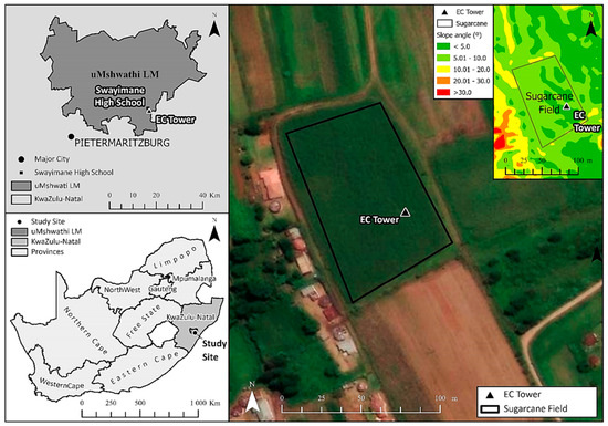
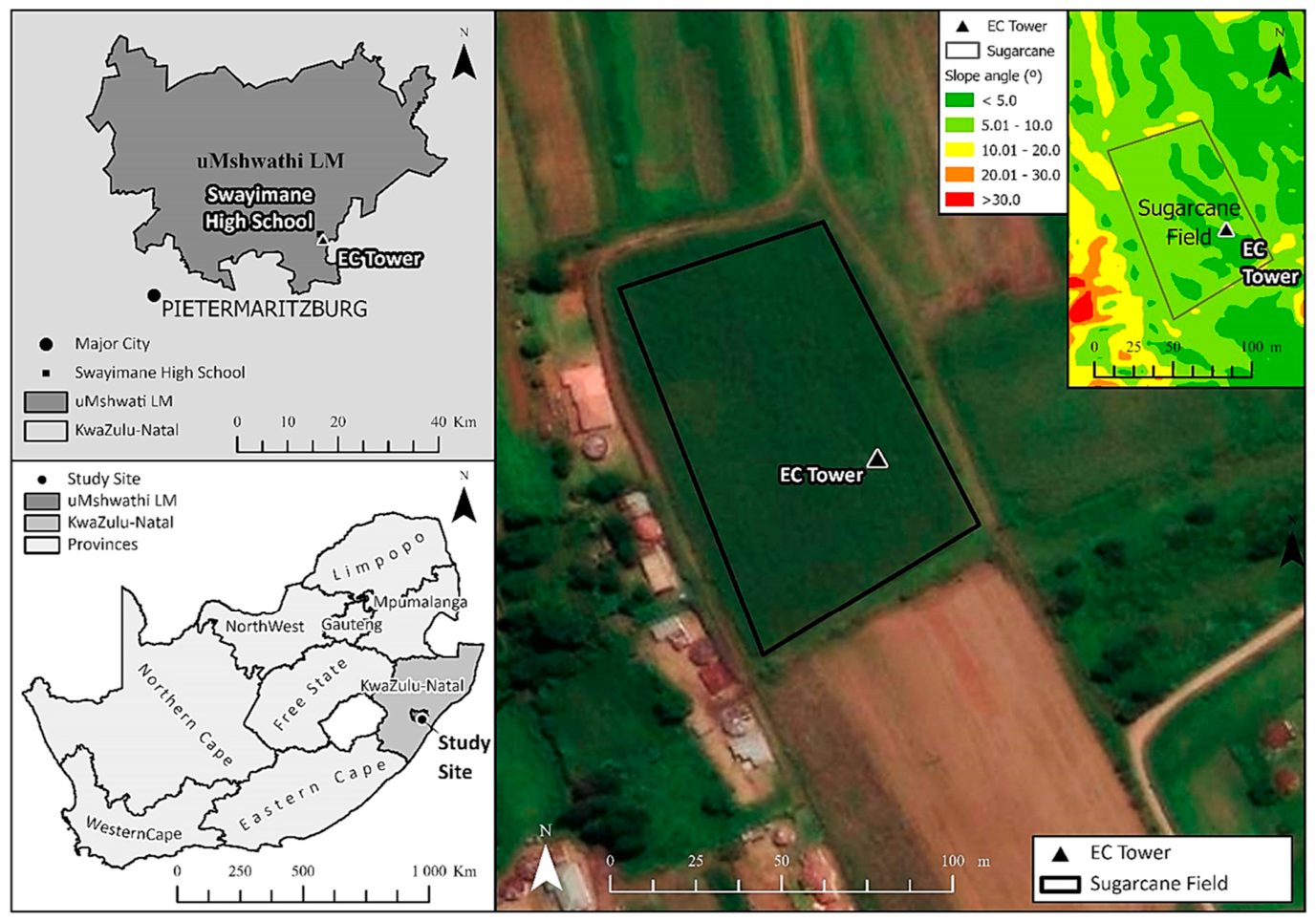
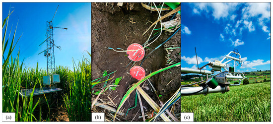
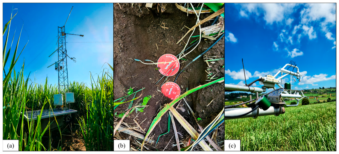
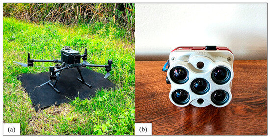
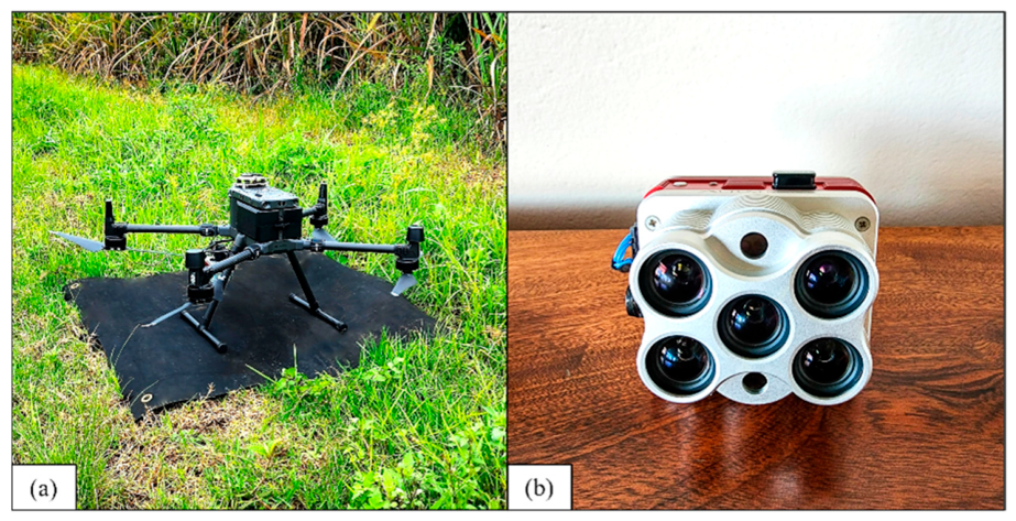
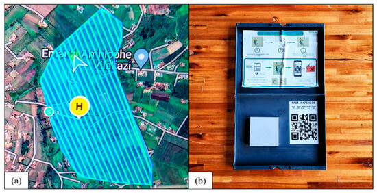
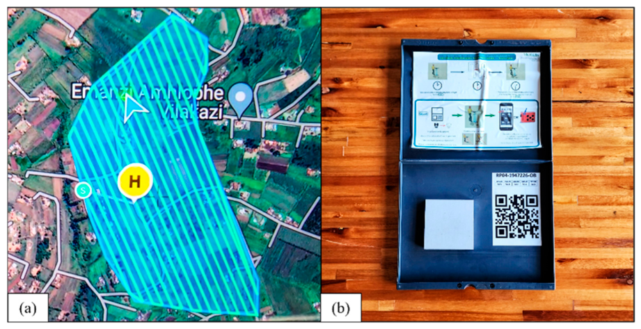
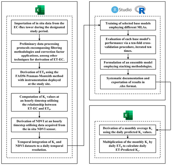
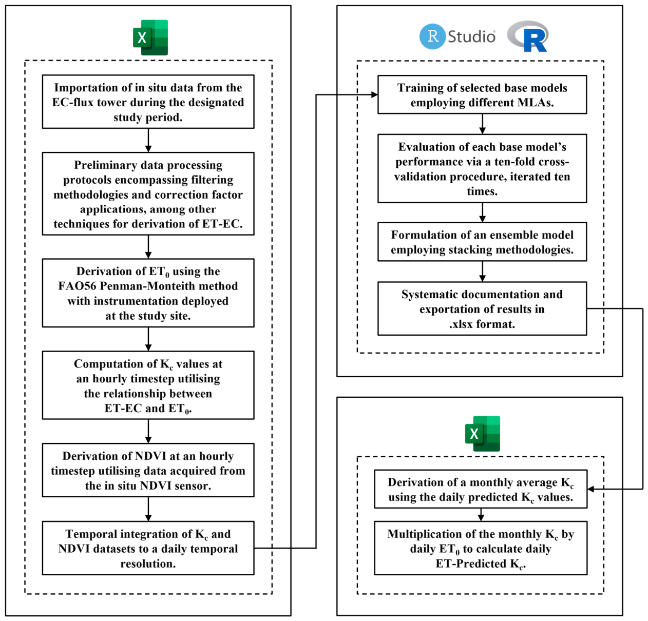
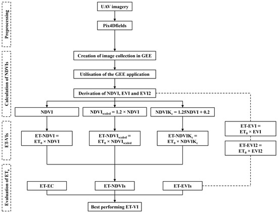
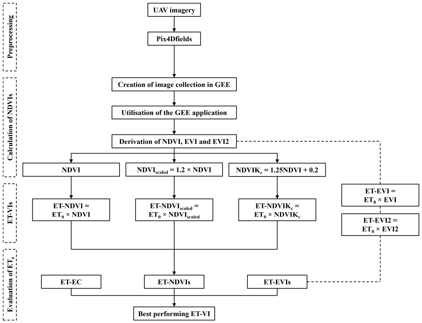
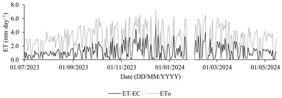
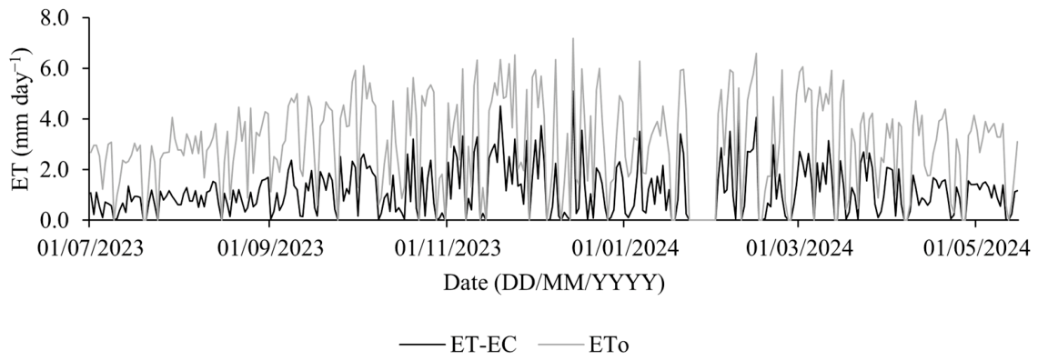
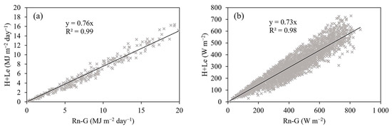
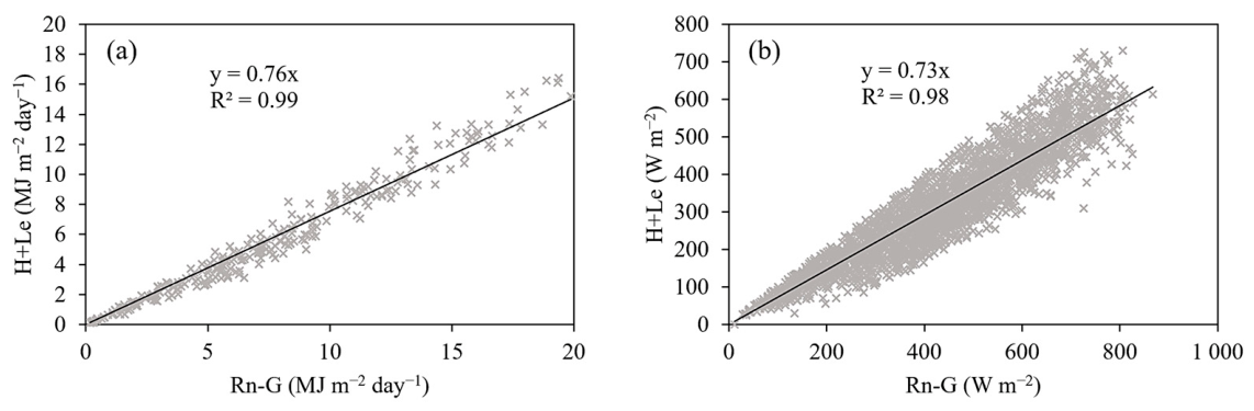
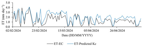
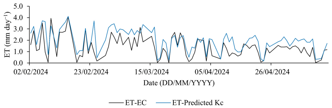
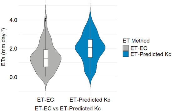
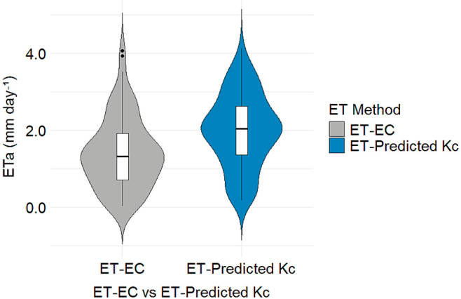
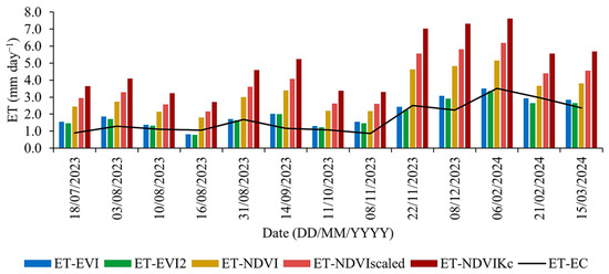
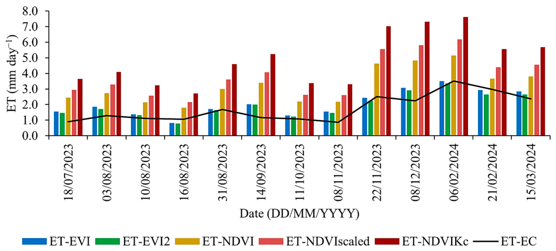
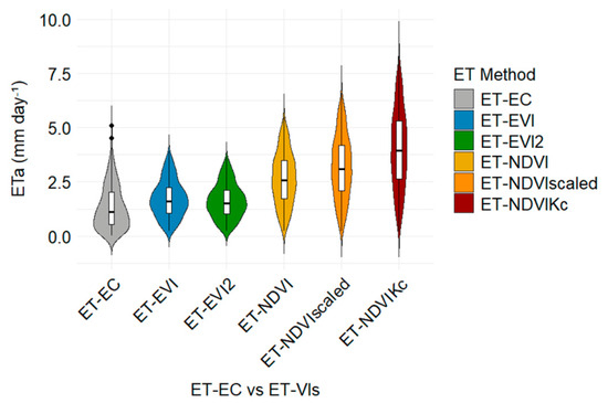
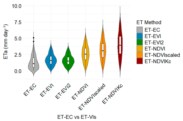
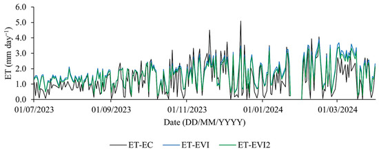
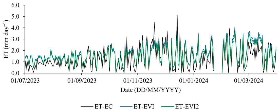
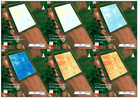
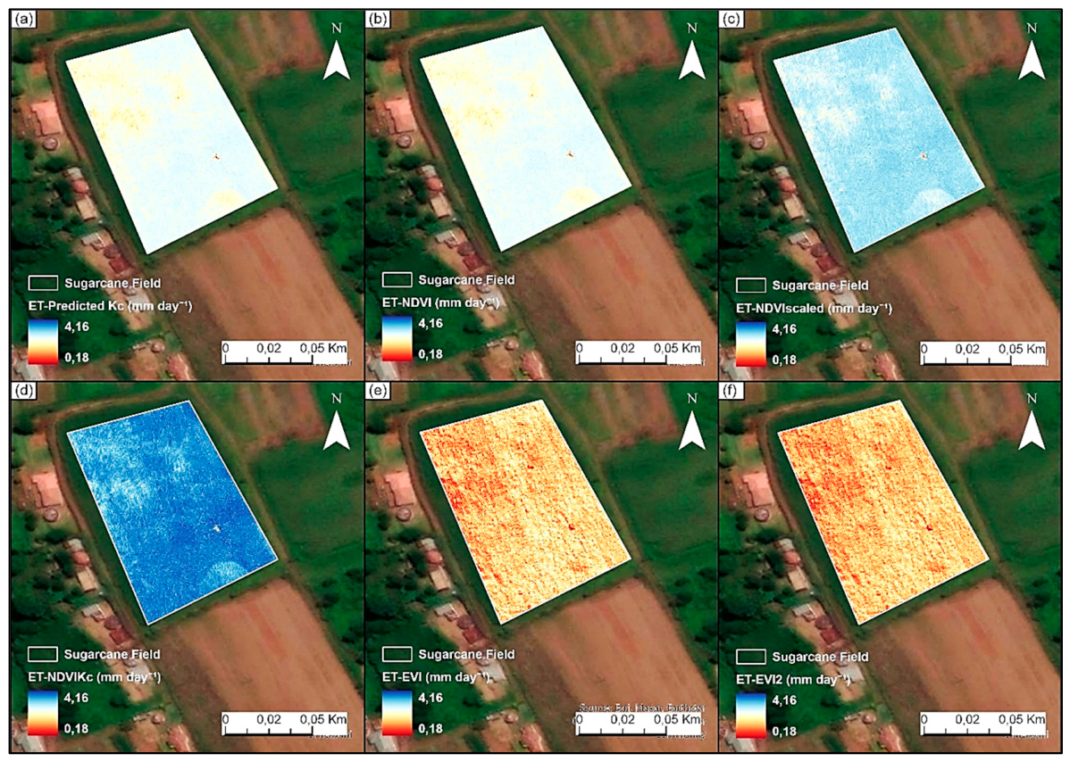
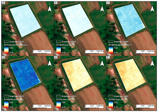
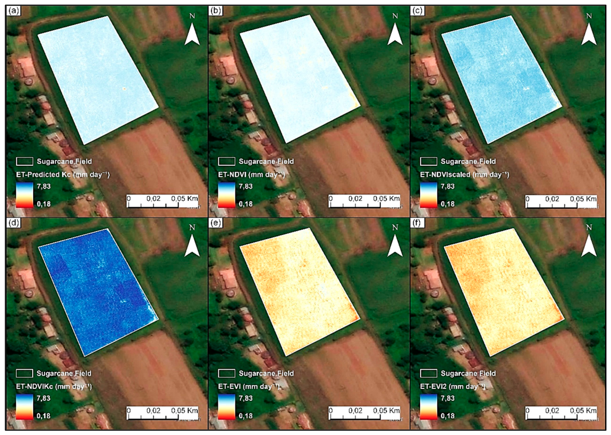

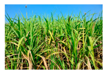
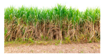
Disclaimer/Publisher’s Note: The statements, opinions and data contained in all publications are solely those of the individual author(s) and contributor(s) and not of MDPI and/or the editor(s). MDPI and/or the editor(s) disclaim responsibility for any injury to people or property resulting from any ideas, methods, instructions or products referred to in the content. |
© 2026 by the authors. Licensee MDPI, Basel, Switzerland. This article is an open access article distributed under the terms and conditions of the Creative Commons Attribution (CC BY) license.