Dynamic Assessment of Near-Surface Icing Risk in High-Mountain Regions Using Multi-Source Remote Sensing and an Energy–Moisture Coupling Model

Highlights

What are the main findings?

• A machine learning method incorporating the CAP index (Cold-Air Pooling index) and physical constraints (PIML-LST, Physics-Informed Machine Learning for Land Surface Temperature) was developed, enabling the reconstruction of daily minimum land surface temperature at 250 m resolution under all weather conditions and successfully eliminating the systematic overestimation of valley temperatures.
• High icing risk areas were found not to correspond simply to the highest elevations or coldest locations, but rather to occur primarily in topographically constrained zones where low-temperature persistence, moisture supply, and freeze–thaw transitions co-occur.

What are the implications of the main findings?

• High icing risk areas were found not to correspond simply to the highest elevations or coldest locations, but rather to occur primarily in topographically constrained zones where low-temperature persistence, moisture supply, and freeze–thaw transitions co-occur.
• The high-resolution risk products provide a terrain-resolved and physically interpretable screening layer for data-scarce alpine environments, which may help identify potential high-risk corridors for winter traffic safety management and agricultural frost risk assessment.

Abstract

In summary, near-surface icing risk in complex alpine terrain is jointly controlled by freezing conditions, moisture supply, freeze–thaw transitions, and topographic energy processes. Traditional approaches relying on sparse station data or single temperature thresholds fail to capture spatial heterogeneity, and frequent cloud cover together with topographic errors severely limit the application of thermal infrared remote sensing. Taking the area along the Duku Highway in the Tianshan Mountains as the study region, a daily icing risk assessment framework at 250 m resolution was constructed using multi-source remote sensing, ERA5-Land reanalysis data, topographic correction, and an energy–moisture dual-constrained model. A diurnal temperature cycle model, the CAP index, and physics-constrained machine learning were integrated to reconstruct the daily minimum land surface temperature ($T_{s,\mathrm{m}\mathrm{i}\mathrm{n}}$) at 250 m resolution under all weather conditions. A probabilistic two-tier risk assessment model was then established by incorporating moisture, topography, and freeze–thaw transitions. The results show that high-risk zones occur primarily in valleys and topographically constrained corridors rather than the coldest elevations. Validation against Landsat LST (r = 0.886) and the Bayanbulak station (bias −0.76 °C, RMSE 5.62 °C, r = 0.91) confirms spatial and seasonal accuracy. Sensitivity and Monte Carlo analyses indicate the RiskScore is mainly controlled by the low-temperature weight, while upstream parameters are less influential. The framework is best applied as a screening and early-warning product to identify sub-kilometer potential icing corridors, complementing point measurements and short-range forecasts.

1. Introduction

Near-surface icing converts cold waves, snowfall, snowmelt refreezing and local terrain effects into direct risks to transport, agriculture and pastoral production. It is therefore one of the most damaging compound meteorological hazards in high-cold mountainous areas. In recent years, mountainous regions of Xinjiang have been frequently impacted by snowstorms and intense cold-air processes [1,2,3,4]. Hazards such as road icing, agricultural frost and snow–ice disasters in pastoral areas have occurred continuously [5,6,7,8,9,10]. As a typical vulnerable area within Xinjiang, the Tianshan Mountains feature dramatic topographic relief, large elevation gradients, long-duration winter snow cover and persistent freeze–thaw processes. Meanwhile, regional warming presents an evident elevation-dependent pattern [11,12]. Collectively, these conditions lead to prominent spatial heterogeneity in near-surface icing risk. Unlike icing over plains, mountain icing is not controlled simply by increasing elevation or decreasing air temperature. It is jointly shaped by weather processes, land surface thermal conditions, water supply, terrain shading and cold-air pooling. Therefore, refined identification of icing risk in sparsely observed and topographically complex mountain environments remains an important scientific challenge for disaster prevention and mitigation in alpine regions.

The core of icing risk assessment is to determine whether low temperatures, water availability and sustained negative energy conditions occur at the same time near the surface. Near-surface thermal conditions provide the basis for freezing. Land surface temperature (LST) reflects the radiative thermal state of the land surface. Surface air temperature (Ta) directly affects freezing diagnosis and road weather risk assessment. Although LST and Ta are linked through the surface energy balance, they are not interchangeable in high-cold mountainous areas. Previous studies have shown that the LST-Ta relationship is affected by season, diurnal cycle, cloud conditions, snow cover, wind speed, humidity, land cover and terrain geometry [13,14,15,16]. In addition, mountain Ta does not always conform to a stable lapse rate, as cold-air pooling, valley temperature inversions and terrain shading render valley bottoms, depressions and enclosed basins prone to freezing earlier than their adjacent slopes [17,18,19,20,21,22,23]. These findings indicate that icing risk identification in the Tianshan Mountains cannot rely only on a single air-temperature threshold or a simple elevation correction. It must also characterize land surface thermal conditions, near-surface air temperature variability and local terrain-induced cooling.

However, current data and methods are still insufficient for fine-scale assessment of near-surface icing risk in high-cold mountainous areas [24,25]. On the one hand, MODIS LST provides frequent observations and continuous regional coverage. It has been widely used to monitor land surface thermal conditions [26,27]. Yet thermal infrared remote sensing cannot provide valid observations under cloud cover [27,28]. In the Tianshan Mountains, cloud, fog and snowfall occur frequently in winter and spring, together with prominent terrain shadow effects. As a result, periods with high icing risk often coincide with the poorest LST observation quality and the most severe data gaps. Existing LST reconstruction methods include spatiotemporal interpolation, statistical regression, multi-source fusion, reanalysis-assisted gap filling and machine learning [28,29,30,31,32,33]. However, extrapolation uncertainty remains high under persistent cloud cover, limited clear-sky samples and strong terrain heterogeneity. For high-cold mountain highway corridors, LST reconstruction should not be limited to filling missing values but preserve spatial continuity and physical plausibility across imbalanced elevation samples and complex terrain-driven energy differences, so as to provide reliable all-weather land surface thermal constraints for icing risk identification.

On the other hand, even when relatively continuous land surface thermal information is available, existing icing risk methods still have limitations in spatial extrapolation and process representation in complex mountains. Previous studies have mainly focused on point-based monitoring, road surface condition recognition and operational early warning. Embedded, roadside and vehicle-mounted sensors can measure road surface temperature, humidity, friction, dielectric properties, optical responses and image information [34,35,36,37,38,39,40,41,42,43,44,45,46]. Deep learning and vision-based models have also improved the automatic recognition of snow cover, slush, ice and black ice [47,48,49,50,51,52,53,54,55,56]. Physical road weather models and statistical warning models estimate road surface temperature, slippery conditions or icing probability from meteorological forcing, supporting road weather information systems and maintenance decisions [25,34,57,58,59]. Such studies provide an important basis for local icing detection and short-term warning. However, their application often depends on dense ground observations, local parameter calibration, or specific road scenarios, which limits their regional transferability in sparsely observed mountain areas. This problem is especially clear in the Tianshan Mountains, where road corridors are narrow and long, elevation gradients are large, slope aspects vary strongly and cold-air pooling occurs frequently. Meteorological station data, road surface sensors, visual recognition results or single-factor thresholds alone cannot continuously describe the low-temperature background, water supply and sustained negative energy constraints required for ice formation. They also cannot fully represent how terrain cold pools, terrain shading and local thermal contrasts modulate near-surface freezing conditions.

Therefore, complex high-cold mountainous regions still lack a near-surface icing risk assessment framework that integrates all-weather thermal state reconstruction, terrain-modulated freezing diagnosis and hydrothermal coupling. To address this gap, the area surrounding the Duku Highway in the Tianshan Mountains is selected as a representative study region, and a fine-scale method for assessing near-surface icing risk is developed by integrating multi-source remote sensing data, ERA5-Land reanalysis data, terrain factors, and land surface environmental information. Within this framework, physics-informed machine learning (PIML) is used to reconstruct all-weather LST under cloud-covered conditions, while terrain correction and cold-air pooling (CAP) adjustment are incorporated to improve the diagnosis of near-surface freezing conditions. Temperature fields, moisture conditions, and energy constraints are further coupled to construct an icing risk index with physical interpretability and uncertainty representation. The proposed framework provides a methodological reference for fine-scale assessment of near-surface icing hazards in alpine mountain regions and supports transport safety, agricultural protection, and disaster risk reduction in cold-region mountain environments.

2. Materials and Methods

2.1. Study Area

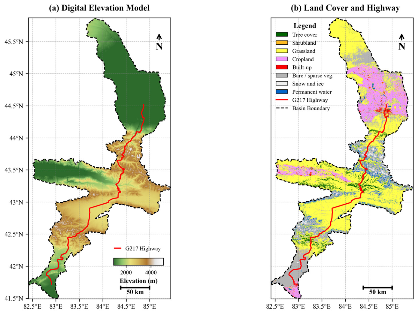
The Tianshan Mountains, a key Central Asian mountain system stretching across Eurasia’s interior and known as the “Central Asian water tower” [60], play a central role in arid-region hydrological cycles and are a typical inland arid alpine system. The study area in central Tianshan covers the Duku Highway’s core drainage basin and surrounding river valley agricultural zones (Figure 1), with rugged terrain, pronounced vertical zonation, and large elevation gradients causing significant spatial heterogeneity [61].

Tianshan’s climate, controlled by westerly circulation and temperate continental conditions with strong topographic vertical differentiation, has a 5 °C annual average air temperature (winter < −10 °C, summer > 15 °C), decreasing linearly with elevation [62]. Annual precipitation (250–300 mm) is spatially uneven, with windward slopes receiving more [63] (over 800 mm in high mountains), and concentrated in spring–summer. High elevations have dominant solid precipitation [64]; the well-developed cryosphere is controlled by air temperature and LST [65]. Tianshan’s complex terrain and cold climate lead to prominent near-surface icing/low-temperature hazards, causing highway blockages [66,67] and late-spring frosts that damage agriculture [6]. The Duku Highway, affected by high elevation, steep slopes, and complex terrain, is prone to cold-air stagnation and intense radiative cooling, increasing near-surface icing frequency. Tianshan’s southern/northern foothills and intermontane valleys are core Xinjiang high-value fruit/forestry zones; spring cold-air accumulation in low elevations causes abrupt temperature drops, triggering severe late-spring frosts. Thus, Tianshan is an ideal natural laboratory for high-resolution dynamic icing risk assessment under complex terrain. The study period includes three 2022–2025 icing seasons (1 October–31 May, ~244 days each).

2.2. Data Sources and Preprocessing

A multi-source data system (Table 1) including meteorological forcing, surface response, and topographic control was constructed. Hourly variables, including thermal states, wind dynamics, precipitation/snowfall and surface radiation fluxes, were extracted from the ERA5-Land high-resolution reanalysis product, which has a native horizontal resolution of approximately 0.1° (~9 km at this latitude). Standardized physical unit conversions were applied to the extracted data. The hourly data were subsequently converted into daily means, daily extremes and daily accumulations. To support the seasonal parameterization of a diurnal temperature cycle (DTC) model, complete 24-hourly sequences were extracted for 56 representative days (7 days per month) across the autumn, winter and spring seasons.

Surface response variables were from Terra MODIS Collection 6.1: 1 km MOD11A1 provided daytime (~10:30) and nighttime (~22:30) LST. Bit-flag quality control (QC) retained only high-quality pixels (retrieval error ≤ 2 K). MOD10A1 (500 m) and MCD43A3 (500 m) characterized snow cover and albedo, respectively; snow cover was binarized via a 50% normalized difference snow index (NDSI) threshold, and shortwave broadband albedo was used directly in energy balance calculations.

Topographic predictors (slope, aspect, TPI, TWI) were extracted from a 30 m SRTM v3 digital elevation model (DEM). Land cover was from 10 m ESA WorldCover 2021, dominated by grassland (42%), bare land/sparse vegetation (28%), snow/ice (12%), and forest (11%).

All variables were resampled to 250 m (WGS84) to resolve spatial scale discrepancies, balancing data limitations, computational efficiency and topographic preservation. The 250 m grid was used as a terrain-consistent modeling grid rather than as evidence that the original temperature datasets contain independent 250 m thermal information. In this framework, the low-frequency thermal background is constrained mainly by MODIS LST and ERA5-Land variables, whereas sub-grid spatial differentiation is introduced through high-resolution terrain and land-surface predictors, including elevation, slope, aspect, terrain shading, cold-air-pooling potential and land cover information. Thus, the 250 m product should be interpreted as a terrain-adjusted spatial allocation of the coarser thermal field, not as a direct 250 m temperature observation. This resolution was selected as a compromise between preserving mountain topographic variability and avoiding the false precision that would result from downscaling to much finer grids, such as 30 m or 100 m. Resampling and aggregation were performed according to variable type and native resolution. Continuous thermal and meteorological variables from ERA5-Land and MODIS were resampled to 250 m using bilinear interpolation. Fine-resolution terrain variables, including DEM-derived elevation, slope, aspect, and TWI, were aggregated by averaging all source pixels within each target cell, whereas land cover was aggregated using the majority class. Nonlinear terrain indices, including CAP and TPI, were first calculated at the native DEM resolution and then aggregated to 250 m to preserve sub-grid terrain variability.

A differentiated topographic downscaling strategy addressed coarse meteorological data–terrain mismatch: air temperature included seasonal lapse rate, surface thermal offset, and CAP correction to capture valley temperature inversions; surface radiation was corrected via terrain radiation factors based on slope and aspect, recovering micro-topographic shading and illumination patterns; wind field was adjusted using TPI to characterize ridge wind acceleration and valley deceleration. Precipitation was bilinearly interpolated (assumed uniform in 9 km grids). Micro-scale precipitation/humidity variability (e.g., leeward rain shadow) was uncharacterized, a priority for future improvement. Post-downscaling, flux variables underwent regional mass conservation checks to ensure multi-scale physical consistency.

To evaluate the physical consistency and reliability of model products, a multi-source satellite validation dataset (thermal infrared, microwave, optical remote sensing) was constructed, covering three cold seasons (consistent with risk products) for cross-validation. The Landsat 8/9 ST_B10 product (100 m) was used as the ground truth for temperature field reconstruction, subjected to QA masking and conversion to °C to generate monthly median products with the DOY band retained. Sentinel-1 GRD IW mode data (100 m) were selected as a proxy for frozen state; descending data were filtered to extract the VV-polarization backscatter coefficient, complementing the limitations of optical/thermal infrared observations. The NDSI_Snow_Cover band (500 m) of MODIS MOD10A1 was binarized with NDSI ≥ 10, and monthly snow cover frequency was calculated to test the model’s ability to characterize snow persistence and its impact on icing risk.

To provide an independent ground-based check on the reconstructed near-surface temperature field, hourly 2 m air temperature and daily minimum temperature observations from the Bayinbuluk meteorological station were obtained from the NOAA ISD-Lite surface observation database. The station is located at approximately 83°43′E, 42°53′N, with an elevation of about 2470 m, and lies within the Duku Highway corridor. These observations were not used for model training and were reserved for independent validation of the modeled ${\mathrm{T}\mathrm{a}}_{\mathrm{C}\mathrm{A}\mathrm{P}}$ product.

To ensure the objectivity and scientific rigor of the validation results, this study constructed a validation dataset based on real-world traffic conditions. The data were sourced from operational traffic bulletins issued by the traffic management authorities of the Xinjiang Uygur Autonomous Region between 2022 and 2025. This dataset encompasses key events such as road closures, speed limits, and driving warnings triggered by road icing, frost, and black ice. By performing keyword searches on raw bulletin records (including “icing”, “frost”, “black ice” and “freezing”) and matching them with the G217 (Duku Highway) network information, a total of 9 candidate events were screened. Validation metrics were calculated within a 500 m buffer zone along the G217 route. Derived from traffic bulletins, this dataset serves as event-level evidence of icing occurrence, primarily reflecting the existence of icing phenomena rather than pixel-scale observational data. Consequently, the evaluation assesses the spatiotemporal correspondence between the model’s high-risk warnings and reported icing events as evidence of screening-level utility, rather than operational reliability or purely physical parameter accuracy.

2.3. Technical Workflow

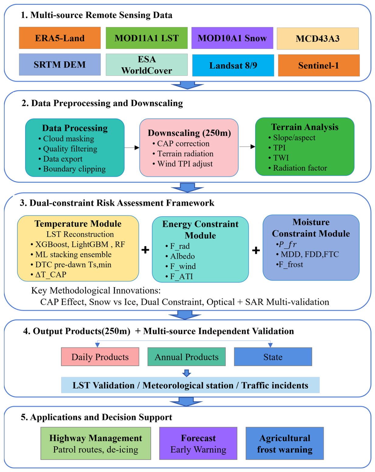
To accurately characterize the spatiotemporal evolution of near-surface icing hazards in complex mountainous regions, a dynamic icing risk assessment framework was developed (Figure 2). A machine learning algorithm incorporating physical constraints was constructed to achieve continuous high-resolution LST retrieval through the deep fusion of ERA5 reanalysis meteorological data and MODIS thermal infrared data. A CAP index and a topographic radiation correction term were introduced to formulate an energy balance module, which corrects temperature estimation biases induced by temperature inversions and slope–aspect radiation differences over complex terrain. A two-tier risk assessment scheme was subsequently established: thresholds were defined based on dynamic freezing point and moisture phase change conditions, and weighting corrections were applied to account for topographic control effects such as thermal inertia delay and cold pool intensification. By explicitly coupling the surface energy budget, moisture dynamics, and topographically driven processes, and by deeply integrating physical mechanisms with machine learning methods, the physical realism of the assessment results was substantially enhanced.

2.4. Methods

2.4.1. Terrain Analysis and Cold-Air Pooling

Topographic factors, including slope, aspect, topographic position index ($TPI$), and topographic wetness index ($TWI$), were derived from the SRTM DEM. To quantify the cooling effect in valleys, a cold-air pool (CAP) index is constructed as:

$$CAP={\alpha }_1·f_{TPI}+{\alpha }_2·(1-Z_{rel})$$

(1)

where initial equal weights are adopted (${\alpha }_1=0.5, {\alpha }_2=0.5$). The topographic position index ($TPI$) was used to represent the relative vertical position of each pixel within its surrounding terrain. The factor $f_{TPI}$ characterizes the degree of topographic depression and is used to represent the enhanced cold-air-pooling potential in valleys and local depressions:

$$f_{TPI}=min\left({\displaystyle \frac{\mathrm{m}\mathrm{a}\mathrm{x}(-TPI,0)}{TP{I}_{scale}}},1\right)$$

(2)

where ${TPI}_{scale}$ is the scaling parameter used to normalize the magnitude of negative $TPI$ values. In this formulation, $\mathrm{m}\mathrm{a}\mathrm{x}(-TPI,0)$ retains depression signals and removes positive TPI values, whereas the outer $\mathrm{m}\mathrm{i}\mathrm{n}(·,1)$ caps the normalized value at 1. In this study, the 5th, 50th and 95th percentiles of $TPI$ calculated over the study domain were approximately (−180), (−12), and (+147) m, respectively. The corresponding 5th, 50th and 95th percentiles of max($-TPI$, 0) were approximately 0, 12, and 180 m. The normalization parameter ${TPI}_{\mathrm{s}\mathrm{c}\mathrm{a}\mathrm{l}\mathrm{e}}$ was set to 300 m, which allows moderate depressions to receive proportional CAP enhancement while restricting $f_{\mathrm{T}\mathrm{P}\mathrm{I}}$ values close to 1 to the most deeply incised valleys and basins. The spatial scale of the moving window for $TPI$ calculation is set to 1000 m. The relative elevation factor $Z_{rel}$ was used to represent the vertical position of each pixel within its surrounding terrain:

$$Z_{rel}={\displaystyle \frac{Z-Z_{min,local}}{Z_{max,local}-Z_{min,local}}}$$

(3)

where $Z_{min,local}$ and $Z_{max,local}$ are the minimum and maximum elevations within a 2 km moving window, respectively. The 2 km window was selected to capture valley–slope elevation contrasts at a broader local terrain scale than the $TPI$ calculation. In this framework, $TPI$ and $Z_{rel}$ represent complementary terrain controls on cold-air pooling: $TPI$, calculated with a 1 km neighborhood, identifies local depressions and concave terrain, whereas $Z_{rel}$, calculated with a 2 km window, describes whether a pixel is located near the valley bottom, mid-slope, or upper terrain within a broader neighborhood. Finally, the CAP-induced temperature correction ($\mathrm{\Delta }{T}_{CAP}$) is implemented as:

$$\mathrm{\Delta }{T}_{CAP}=-{\beta }_{CAP}·CAP·f_{time}\left(t\right)·I_{stable}$$

(4)

where ${\beta }_{CAP}$ represents the maximum temperature drop amplitude, empirically set to $5.0 °\mathrm{C}$, within the range of nocturnal valley cold-pool and inversion strengths reported in mountain studies [21,68]. CAPs primarily develop under conditions of clear skies, light winds, and nocturnal radiative cooling; their effect is significantly stronger at night. Therefore, a nocturnal enhancement factor, $f_{time}\left(t\right)$, was applied to account for the valley inversion life cycle (18:00–06:00, factor 1.0; 06:00–09:00, factor 0.3(9 − t)/3; 09:00–18:00, factor 0.0) [20,69]. Furthermore, because CAP formation is favored by stable boundary-layer conditions, an atmospheric stability indicator, $I_{stable}$, was introduced to represent the suppression of CAP under cloudy or windy conditions [18,21]. Based on previous studies and empirical parameterization, $I_{\mathrm{s}\mathrm{t}\mathrm{a}\mathrm{b}\mathrm{l}\mathrm{e}}$ was set to 1.0 for clear/calm nights and to 0.3–0.5 for cloudy or windy nights. The background winter lapse rate, ${LAPSE}_{winter}$ = 0.0050 °C/m, was used for elevation extrapolation, while valley inversions were represented separately by the CAP correction, consistent with weak or inverted near-surface winter lapse rates in the Tianshan [17].

2.4.2. Temperature Field Construction

The extensive data gaps in thermal infrared remote sensing LST caused by cloud cover represent a core challenge for temperature field reconstruction in mountainous areas. This challenge was addressed through a synergistic retrieval strategy combining clear-sky observations with cloud-gap reconstruction. The ERA5 air temperature (with an original spatial resolution of ~9 km) was downscaled to 250 m via a multi-factor correction approach:

$$T_{a,fine}=T_{a,ERA5}-\mathrm{\Gamma }\left(m\right)·\mathrm{\Delta }Z+\mathrm{\Delta }{T}_{CAP}$$

(5)

where $\mathrm{\Gamma }\left(m\right)$ is the seasonal temperature lapse rate. Based on characteristic mountain environments [70], the values for winter, spring, summer, and autumn were empirically set to 0.5, 0.55, 0.65, and 0.55 °C/100 m, respectively. $\mathrm{\Delta }Z$ is the elevation difference calculated as $\mathrm{\Delta }Z=Z_{fine}-Z_{coarse}$, where $Z_{coarse}$ and $Z_{fine}$ correspond to ERA5-Land geopotential/g and the 250 m DEM. $\mathrm{\Delta }{T}_{CAP}$ is the cold-air pool correction term derived from Equation (4). Furthermore, the physical reconstruction of land surface temperature (LST) under cloudy conditions is formulated as:

$$T_{s,cloudy}=T_{skin,ERA5}-\mathrm{\Gamma }\left(m\right)·\mathrm{\Delta }Z+\mathrm{\Delta }{T}_{LC}+\mathrm{\Delta }{T}_{CAP}$$

(6)

where $\mathrm{\Delta }{T}_{LC}$ denotes the land cover-dependent temperature offset (Table 1).

Table 1. Land cover temperature offsets.

Land Cover	Code	Temperature Offset ΔT (°C)	Physical Mechanism
Forest	10	0	Combined effect of canopy shading and transpiration cooling [71]
Shrubland	20	0.5	Warming effect of sparse vegetation
Grassland	30	1	Reference baseline
Cropland	40	1.5	Lower thermal inertia
Built-up	50	3	Urban heat island effect; high heat storage capacity of asphalt/concrete
Bare land	60	2	Strong daytime warming due to low thermal inertia
Snow/ice	70	−5	Strong cooling due to high albedo and thermal insulation effects [72]
Water	80	0	High heat capacity
Wetland	90	0.5	Combined effect of evaporative cooling and soil moisture

Table 1. Land cover temperature offsets.

Land Cover	Code	Temperature Offset ΔT (°C)	Physical Mechanism
Forest	10	0	Combined effect of canopy shading and transpiration cooling [71]
Shrubland	20	0.5	Warming effect of sparse vegetation
Grassland	30	1	Reference baseline
Cropland	40	1.5	Lower thermal inertia
Built-up	50	3	Urban heat island effect; high heat storage capacity of asphalt/concrete
Bare land	60	2	Strong daytime warming due to low thermal inertia
Snow/ice	70	−5	Strong cooling due to high albedo and thermal insulation effects [72]
Water	80	0	High heat capacity
Wetland	90	0.5	Combined effect of evaporative cooling and soil moisture

MODIS thermal infrared remote sensing LST products are severely affected by cloud cover; in the Tianshan Mountains, the cloud coverage rate during winter and spring can reach 40–60% (based on our statistical analysis of original MODIS LST observations for the study period), resulting in extensive LST data loss. For cloud-covered pixels, LST was reconstructed using a physics-guided ensemble machine learning approach that integrates ERA5-Land meteorological variables, terrain factors, vegetation indices, land cover information, and temporal cycle features. XGBoost [73], LightGBM [74], and Random Forest [75] were used as base learners, and their outputs were combined using a ridge regression meta-learner. The under-cloud LST was reconstructed by a stacking ensemble of these three learners (150–200 trees, depth 6–20) with a ridge meta-learner, trained separately for each day on that day’s cloud-free MODIS nighttime LST pixels (≈500 to 4.7 × 10⁵ per day, capped at 50,000). Accuracy was evaluated with spatial block GroupKFold (5 folds, 50 × 50-pixel blocks) to avoid spatial autocorrelation leakage. On held-out pixels, the ensemble reaches RMSE = 1.90 K, MAE = 1.29 K and R² = 0.99, with the ERA5 thermal field, elevation, and the day-of-year cosine the leading predictors (ΔRMSE ≈ 0.64, 0.26 and 0.13 K). As the surface temperature beneath clouds is unobserved, this held-out clear-sky error is the proxy for under-cloud accuracy. Clear-sky and under-cloud fusion:

$$T_s=\left\{\begin{array}{c}{T}_{MODIS},QC=good\\ T_{s,cloudy},cloudy/poor-quality\end{array}\right.$$

(7)

Specifically, MODIS nighttime LST pixels with “QC_Night” bits 0–1 = 00 and an LST error flag $\backslash \mathrm{l}\mathrm{e}$ 2 K are defined as reliable clear-sky observations. Pixels with a value of 2 for bits 0–1 (binary 10) are defined as missing data due to cloud contamination. The remaining pixels—whether produced but of lower quality or not produced for other reasons—are categorized as poor-quality and are incorporated into the under-cloud reconstruction process. If the machine learning (ML) enhancement is triggered, the fusion logic is updated as follows:

$$T_s=\left\{\begin{array}{c}{ T}_{MODIS},QC=good\\ T_{ML},cloudy,n_{clear}\ge n_{min},{\sigma }_{ML}\le {\sigma }_{max}\\ T_{s,cloudy},otherwise\end{array}\right.$$

(8)

To capture the relationships between cloud-obscured LST and environmental conditions, we selected variables related to surface energy balance, topographic modulation of microclimate, and seasonal and spatial heterogeneity. This resulted in a 25-dimensional feature space (

Table 2. Feature variables for under-cloud LST reconstruction.

Category	Variable	Physical Meaning	Data Source
Meteorological	$T_{skin}$	Skin temperature	ERA5-Land (~9 km)
	$T_{2m}$	2 m air temperature	ERA5-Land
	$Td$	2 m dewpoint temperature	ERA5-Land
	SSRD	Surface solar radiation downwards	ERA5-Land
	STRD	Surface thermal radiation downwards	ERA5-Land
	SP	Surface pressure	ERA5-Land
	$U_{wind}$	10 m wind speed	ERA5-Land
Topographical	Z	Elevation	SRTM (30 m)
	$\beta$	Slope	SRTM-derived
	$\mathrm{c}\mathrm{o}\mathrm{s}\left(\alpha \right),\mathrm{s}\mathrm{i}\mathrm{n}\left(\alpha \right)$	Aspect components	SRTM-derived
	TPI	Topographic position index	SRTM-derived
	CAP	Cold-air pooling index	Calculated in this study
	TWI	Topographic wetness index	SRTM-derived
Temporal	$\mathrm{c}\mathrm{o}\mathrm{s}\left(2\pi d/365\right)$	DOY cosine component	Date-derived
	$\mathrm{s}\mathrm{i}\mathrm{n}\left(2\pi d/365\right)$	DOY sine component	Date-derived
Spatial	${\overline{\mathrm{T}}}_{\mathrm{s}\mathrm{k}\mathrm{i}\mathrm{n}}\left(3\backslash \mathrm{t}\mathrm{i}\mathrm{m}\mathrm{e}\mathrm{s}3\right)$	Neighborhood mean of $T_{skin}$	ERA5-Land
	${\sigma }_{skin}\left(3\backslash \mathrm{t}\mathrm{i}\mathrm{m}\mathrm{e}\mathrm{s}3\right)$	Neighborhood standard deviation of $T_{skin}$	ERA5-Land
Vegetation	NDVI	Normalized Difference Vegetation Index	MODIS (1 km)
Land Cover	$L{C}_i$, $i=1,\dots , 6$	Land cover (one-hot encoding); six feature dimensions	ESA WorldCover

), consisting of 19 continuous or cyclic predictors and six one-hot encoded land cover variables. $L{C}_i(i=1,\dots , 6)$ represents the six ESA WorldCover classes retained in the study area after masking and aggregation. In this study, these classes correspond to tree cover, shrubland, grassland, cropland, bare/sparse vegetation, and snow/ice.

The DOY periodic features [$\mathrm{c}\mathrm{o}\mathrm{s}(2\pi d/365)$, $\mathrm{s}\mathrm{i}\mathrm{n}(2\pi d/365)$] were introduced to capture seasonal LST cycles (avoiding year boundary discontinuity), and the spatial neighborhood features were introduced to enhance topographic adaptability.

For daily LST reconstruction, clear-sky pixels (via MODIS QC) were training samples; the 25-dimensional feature vector was extracted, and the model was trained with clear-sky LST as labels, then applied to cloud-covered pixels to predict LST and uncertainty. Full-coverage LST combined original MODIS (clear sky) and ML predictions (cloudy). Accuracy was validated with Landsat 8/9 (Band 10, 100 m) via same-day, same-pixel matching, using RMSE, MAE, R², and bias.

Regarding the estimation of the DTC and the early morning minimum temperature, it should be noted that the MODIS nighttime overpass time is approximately 22:30, whereas road icing occurs most frequently during the early morning hours before sunrise (approximately 05:00–07:00), resulting in a time lag of 4–8 h. During this period, the LST continues to decrease through radiative cooling. The diurnal variation in LST follows an approximately sinusoidal pattern [76]. Consequently, a DTC model was employed to estimate the early morning minimum LST as follows:

$$T_s\left(t\right)=\overline{T}-A·\cos \left({\displaystyle \frac{2\pi \left(t-t_{min}\right)}{24}}\right)$$

(9)

where $\overline{T}$ is the daily mean temperature, A is half the amplitude of the diurnal temperature range, and $t_{min}$ is the time of the daily minimum temperature (typically around sunrise). Assuming that the diurnal variations in LST and air temperature are in phase, the early morning minimum LST can be estimated as:

$$T_{s,min}=T_{s,22:30}+\mathrm{\Delta }{T}_{ERA5}$$

(10)

$$\mathrm{\Delta }{T}_{ERA5}=T_{ERA5}\left(06:00\right)-T_{ERA5}\left(22:00\right)$$

(11)

To account for the thermal lag characteristics of different underlying surfaces, this estimation is further corrected as follows:

$${\mathrm{T}}_{\mathrm{s},\mathrm{m}\mathrm{i}\mathrm{n}}={\mathrm{T}}_{\mathrm{s},22:30}+\mathrm{\Delta }{\mathrm{T}}_{\mathrm{E}\mathrm{R}\mathrm{A}5}\times {\mathrm{f}}_{\mathrm{l}\mathrm{a}\mathrm{g}}\left(\mathrm{L}\mathrm{C}\right)$$

(12)

where $f_{lag}\left(LC\right)$ is the land cover-dependent thermal lag correction factor (Table 1).

In the risk assessment framework, the condition $T_{s,min}\le T_f$ serves as a critical criterion to determine whether the freezing temperature requirement is met. It plays a vital role in both the calculation of the low-temperature factor and the identification of snowmelt–refreeze cycles.

2.4.3. Energy Constraint Module

To quantify the regulatory role of surface energy balance on near-surface icing processes, this study constructed a comprehensive energy constraint module. This module incorporates terrain radiation ($F_{rad}$), effective snow albedo ($F_{albedo}$), turbulent wind cooling effects ($F_{wind}$), and Apparent Thermal Inertia (ATI). It is designed to quantify the state of surface energy deficit conducive to icing, which arises from conditions of low radiative input, high reflective loss, and weak thermal capacity.

By integrating solar geometric parameters with micro-topographic features (slope, aspect, and sky view factor), the terrain radiation factor ($F_{rad}$) is derived to precisely characterize the spatial heterogeneity in local shortwave radiation balance. Surface solar radiation is significantly regulated by topography. Solar geometry calculations include the solar declination, hour angle, altitude angle, and azimuth angle. The solar declination is defined as:

$$\delta =23.45°\times \mathrm{s}\mathrm{i}\mathrm{n}\left({\displaystyle \frac{360°\times (284+DOY)}{365}}\right)$$

(13)

The terrain radiation factor comprehensively considers both direct and diffuse components:

$$F_{rad}=\mathrm{c}\mathrm{o}\mathrm{s}{\theta }_s\mathrm{c}\mathrm{o}\mathrm{s}\beta +\mathrm{s}\mathrm{i}\mathrm{n}{\theta }_s\mathrm{s}\mathrm{i}\mathrm{n}\beta \mathrm{c}\mathrm{o}\mathrm{s}({\varphi }_s-\varphi )+k_d·SVF$$

(14)

where ${\theta }_s$ is the solar zenith angle, $\beta$ is the slope, ${\varphi }_s$ is the solar azimuth angle, $\varphi$ is the aspect, $k_d$ is the diffuse coefficient, and SVF is the sky view factor.

By coupling the dynamics of snow cover fraction, the effective albedo of the underlying surface ($F_{albedo}$) is calculated to account for the snow albedo effect. The formulas for the comprehensive albedo and albedo factor are as follows:

$${\alpha }_{eff}=f_{snow}·{\alpha }_{snow}+(1-f_{snow})·{\alpha }_{bare}$$

(15)

$$F_{albedo}={\alpha }_{eff}/0.9$$

(16)

Based on the Bulk Aerodynamic Method, a wind cooling factor ($F_{wind}$) is introduced to quantitatively characterize the intensified nocturnal surface heat dissipation driven by high wind speeds enhancing turbulent heat exchange. Wind speed accelerates the turbulent loss of surface heat to the atmosphere. The theoretical relationship between surface sensible heat flux $H$ and wind speed can be expressed as:

$$\mathrm{H}=\mathrm{\rho }·{\mathrm{c}}_{\mathrm{p}}·{\mathrm{C}}_{\mathrm{h}}·\mathrm{U}·\left({\mathrm{T}}_{\mathrm{s}}-{\mathrm{T}}_{\mathrm{a}}\right)$$

(17)

where $\mathrm{\rho }=1.225$ kg/m³ is the air density, ${\mathrm{c}}_{\mathrm{p}}=1005$_p J/(kg·K) is the specific heat capacity at constant pressure, C_h is the heat transfer coefficient, and U is the near-surface wind speed. Since wind speeds in mountainous areas are significantly modulated by topography, a wind speed adjustment based on the topographic position index (TPI) is required:

$$U_{adj}=U\left(1+{\alpha }_{topo}·TP{I}_{norm}\right)$$

(18)

where $TP{I}_{norm}$ is the normalized TPI and ${\alpha }_{topo}$ is the topographic correction coefficient. In this study, the enhancement effect of wind speed on heat exchange is simplified into a wind speed enhancement factor (${\mathrm{F}}_{\mathrm{w}\mathrm{i}\mathrm{n}\mathrm{d}}$):

$${\mathrm{F}}_{\mathrm{w}\mathrm{i}\mathrm{n}\mathrm{d}}=1+{\alpha }_w·\min \left({\displaystyle \frac{U}{{\mathrm{U}}_{\mathrm{r}\mathrm{e}\mathrm{f}}}},1\right)$$

(19)

where $U_{ref}$ = 10 m/s is the reference wind speed, and the wind speed influence coefficient ${\alpha }_w$ is set to 0.3. A lower ${\mathrm{F}}_{\mathrm{w}\mathrm{i}\mathrm{n}\mathrm{d}}$ is more conducive to icing formation. To reflect the thermal buffering characteristics of different land cover types, the Apparent Thermal Inertia (ATI) is derived using the diurnal surface temperature range and surface albedo:

$$ATI={\displaystyle \frac{1-{\alpha }_{eff}}{T_{s,day}-T_{s,night}}},F_{ATI}=1-{\displaystyle \frac{ATI}{max\left(ATI\right)}}$$

(20)

By applying empirical weights, the above four physical indicator factors are reconstructed into a comprehensive energy index ($E_{index}$). This index serves as a constraint to quantitatively characterize the environmental driving force for icing triggered by rapid surface heat loss in alpine regions:

$$E_{index}=w_1(1-F_{rad})+w_2{F}_{albedo}+w_3{F}_{wind}+w_4{F}_{ATI}$$

(21)

Considering the relative contributions of respective flux components in the mountain surface energy balance (SEB) equation, the *a priori* weights for these physical indicators are assigned as $w_1=0.30$, $w_2=0.25$, $w_3=0.25$, and $w_4=0.20$.

2.4.4. Moisture Constraint Module

Sufficient liquid moisture is the material prerequisite for near-surface icing. In this study, a moisture constraint module is constructed to quantify the material basis for icing. The wet-bulb temperature ($T_w$) is calculated based on Stull’s empirical formula [77] to finely classify precipitation phases. Specifically, $T_w>1.5\hspace{0.17em}°\mathrm{C}$ indicates liquid precipitation, $-0.5\hspace{0.17em}°\mathrm{C}<T_w\le 1.5\hspace{0.17em}°\mathrm{C}$ indicates mixed-phase precipitation, and $T_w\le -0.5\hspace{0.17em}°\mathrm{C}$ indicates solid precipitation. Concurrently, the probability of freezing rain ($P_{fr}$) is estimated by combining air temperature conditions:

$$P_{fr}=\left\{\begin{array}{cc}1.0,& T_a<0 °\mathrm{C}\wedge 0<T_w<2 °\mathrm{C}\\ 0.5,& T_a<0 °\mathrm{C}\wedge -1<T_w\le 0 °\mathrm{C}\\ 0,& \mathrm{otherwise}\end{array}\right.$$

(22)

Although freezing rain is relatively rare in Xinjiang, it often results in the most severe icing when it occurs; therefore, the discrimination of this precipitation form is retained. Snowmelt is simulated using a degree-day model, calculating the snowmelt amount based on a degree-day factor and a melting threshold:

$$M=DDF·(T_a-T_{melt}{)}^{+}·\mathrm{\Delta }t$$

(23)

where $DDF=5.0$ mm/(°C·d) is the degree-day factor and $T_{melt}=0 °\mathrm{C}$ is the snowmelt threshold. Finally, the frost deposition potential (${\mathrm{F}}_{\mathrm{f}\mathrm{r}\mathrm{o}\mathrm{s}\mathrm{t}}$) is determined based on the relationship between the surface temperature (${\mathrm{T}}_{\mathrm{s}}$) and the dew point temperature (${\mathrm{T}}_{\mathrm{d}}$):

$$F_{frost}=\left\{\begin{array}{cc}1.0,& T_s<T_d\wedge T_s<0 °\mathrm{C}\\ 0.5,& T_s<T_d\wedge T_s\ge 0 °\mathrm{C}\\ 0,& T_s\ge T_d\end{array}\right.$$

(24)

When $T_s\ge T_d$, the surface is dominated by evaporative dissipation, and the frosting potential is zero. When $T_s<T_d$, satisfying the conditions for water vapor condensation: if the surface temperature is below freezing, near-surface water vapor will directly deposit and crystallize on the road surface or freeze instantaneously after condensation, exhibiting extremely high disaster potential; if the surface temperature remains above freezing, although ice does not form directly, the moisture provides liquid water for potential subsequent freezing during nocturnal cooling, thus regarded as a moderate hazard potential. Precipitation, snowmelt, relative humidity, topographic wetness index (TWI), and frosting potential are normalized and reconstructed into a Comprehensive Moisture Index ($W_{index}$).

$$W_{index}=w_1{F}_{precip}+w_2{F}_{melt}+w_3{F}_{RH}+w_4{F}_{TWI}+w_5{F}_{frost}$$

(25)

An adequate supply of liquid moisture is the material prerequisite for near-surface icing. Based on the hydro-physical mechanisms in mountainous regions, the a priori weights for the respective moisture indicator factors are assigned as follows: $w_1=0.25$, $w_2=0.25$, $w_3=0.15$, $w_4=0.15$, and $w_5=0.20$.

2.4.5. Risk Assessment Framework

A dual-layer risk assessment method is established by combining the judgment of necessary icing conditions with the quantification of risk intensity. Temperature and moisture are the two necessary conditions to determine icing:

$$I_{risk}=\mathbb{I}(T_s\le T_f)\times \mathbb{I}(W>W_{th})$$

(26)

where $T_f$ is the dynamic freezing point temperature (considering underlying surface types, it can be as low as −2 °C in built-up areas), and $W_{th}=0.1$ is the minimum moisture threshold. The quantified icing risk intensity is obtained by weighting five factors: low temperature, energy, moisture, cold pool, and freezing rain:

$$S_{risk}={\beta }_1{F}_{cold}+{\beta }_2{F}_{energy}+{\beta }_3{F}_{moisture}+{\beta }_4{F}_{CAP}+{\beta }_5{F}_{fr}$$

(27)

$$F_{cold}=\mathrm{m}\mathrm{i}\mathrm{n}\left(1,\mathrm{m}\mathrm{a}\mathrm{x}\left(0,{\displaystyle \frac{T_f-T_s}{\mathrm{\Delta }{T}_{ref}}}\right)\right),\mathrm{\Delta }{T}_{ref}=20 °\mathrm{C}$$

(28)

This study employs a physics-constrained weighted scoring method to construct the icing risk index. The initial weights of each factor are set based on the importance of the icing formation mechanism. Specifically, the low-temperature factor (${\beta }_1=0.25$) and moisture factor (${\beta }_3=0.25$) are assigned the highest weights as necessary conditions for icing formation. The freezing rain factor (${\beta }_5=0.20$) is heavily emphasized due to its association with the most hazardous type of icing. The energy factor (${\beta }_2=0.15$) and cold pool factor (${\beta }_4=0.15$) characterize the persistence of cooling and the localized accumulation of cold air in mountainous areas, respectively.

The comprehensive risk score is formulated as:

$$R_{score}=I_{risk}·S_{risk}+\left(1-I_{risk}\right)·\lambda ·S_{risk}$$

(29)

where $\lambda =0.3$is the penalty factor. Based on the normalized comprehensive risk score, an equal-interval threshold method is employed to classify the icing risk into a five-level warning gradient: a score of 0.0–0.2 is defined as no risk (Level 0); the 0.2–0.8 interval is sequentially divided into low (Level 1), moderate (Level 2), and high (Level 3) risk, with a step size of 0.2; and the extreme interval of 0.8–1.0 indicates an extremely high risk state (Level 4).

Given that ground ice evolution exhibits significant temporal continuity and memory effects, this study introduces a Markov State Transition Model to track the complete lifecycle of icing events. The discrete state space of ice evolution is defined as $S=\{S_0:\mathrm{i}\mathrm{c}\mathrm{e}-\mathrm{f}\mathrm{r}\mathrm{e}\mathrm{e},S_1:\mathrm{t}\mathrm{h}\mathrm{i}\mathrm{n} \mathrm{i}\mathrm{c}\mathrm{e}(<2 \mathrm{m}\mathrm{m}),S_2:\mathrm{t}\mathrm{h}\mathrm{i}\mathrm{c}\mathrm{k} \mathrm{i}\mathrm{c}\mathrm{e}(\ge 2 \mathrm{m}\mathrm{m}),S_3:\mathrm{m}\mathrm{e}\mathrm{l}\mathrm{t}\mathrm{i}\mathrm{n}\mathrm{g}\}$. The core transition probability matrix $P$ is dynamically driven by daily meteorological forcing and risk scores. The state transition probability $p_{ij}=P(S_{t+1}=j\mid S_t=i)$ is influenced by the daily risk score, surface temperature variation, and precipitation conditions (

Table 3. State transition conditions.

Current State (${\mathit{S}}_{\mathit{t}}$)	Current State (${\mathit{S}}_{\mathit{t}}$)	Current State (${\mathit{S}}_{\mathit{t}}$)	Current State (${\mathit{S}}_{\mathit{t}}$)
$S_0$ → $S_1$	Ice-free $\to$ Thin ice	$R_{score}>0.5$ and $T_{s,min}<T_f$ and $W>W_{th}$	Initial freezing
$S_1$ → $S_2$	Thin ice → Thick ice	$R_{score}>0.6$ and $T_s<T_f-2 °\mathrm{C}$	Continuous freezing and thickening
$S_1$ → $S_3$	Thin ice $\to$ Melting	$T_s>T_f+2 °\mathrm{C}$	Warming-induced melting
$S_2$ → $S_3$	Thick ice $\to$ Melting	$T_s>T_f$ and $SSRD>200{ \mathrm{W}/\mathrm{m}}^2$	Radiation and warming-induced melting
$S_3$ → $S_0$	Melting $\to$ Ice-free	$T_s>2 °\mathrm{C}$ and No precipitation	Complete evaporation and drying

).

2.4.6. Validation Strategy

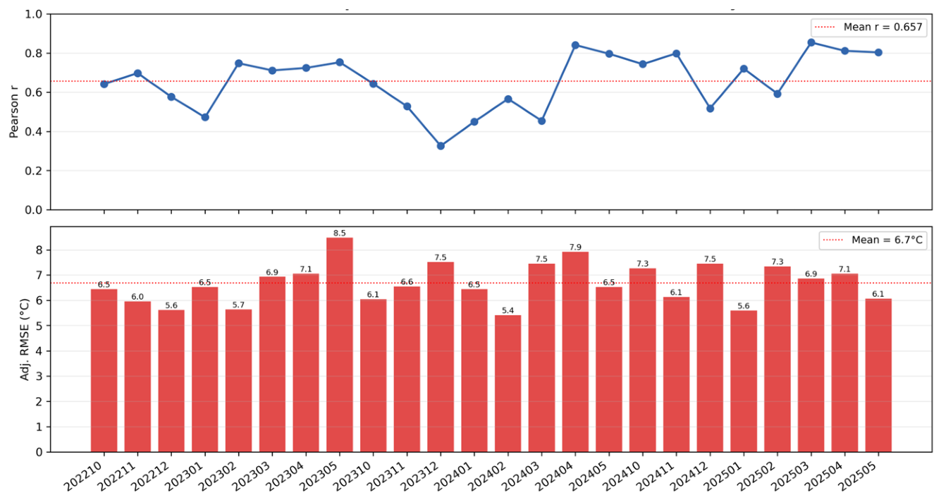
A two-tier validation strategy was adopted to evaluate the physical consistency of intermediate variables and the event detection performance of the final product. First, a validation analysis was conducted using multi-source remote sensing data. Over the 24 cold-season months within the study period, three independent satellite remote sensing variables were cross-compared with corresponding model outputs at the monthly scale and at the pixel level.

The monthly median composite LST derived from the Landsat 8/9 Collection 2 Level-2 thermal infrared band (ST_B10) was used as a reference to evaluate the spatial consistency of the model-reconstructed early morning minimum LST (${\mathrm{T}}_{\mathrm{s},\mathrm{m}\mathrm{i}\mathrm{n}}$). Because ${\mathrm{T}}_{\mathrm{s},\mathrm{m}\mathrm{i}\mathrm{n}}$ represents the pre-dawn minimum temperature while the Landsat overpass time is approximately 10:30 local time, a systematic diurnal temperature difference exists between the two. Therefore, spatial consistency was adopted as the primary evaluation objective, and correlation metrics were used instead of direct error statistics. The Pearson correlation coefficient was used to measure linear spatial correspondence:

$$r={\displaystyle \frac{{\displaystyle {\sum }_{i=1}^n}(T_{s,\mathrm{m}\mathrm{i}\mathrm{n},i}-{\overline{T}}_{s,\mathrm{m}\mathrm{i}\mathrm{n}})(LS{T}_i-\overline{LST})}{\sqrt{{\displaystyle {\sum }_{i=1}^n}(T_{s,\mathrm{m}\mathrm{i}\mathrm{n},i}-{\overline{T}}_{s,\mathrm{m}\mathrm{i}\mathrm{n}}{)}^2{\displaystyle {\sum }_{i=1}^n}(LS{T}_i-\overline{LST}{)}^2}}}$$

(30)

The Spearman rank correlation coefficient ($\rho$) was used to evaluate spatial ranking consistency. In addition, a bias-adjusted RMSE was introduced:

$${\mathrm{RMSE}}_{\mathrm{adj}}=\sqrt{{\displaystyle \frac{1}{n}}{\sum }_{i=1}^n({\mathrm{T}}_{\mathrm{s},\min ,\mathrm{i}}-({\mathrm{LST}}_i-\overline{\mathrm{\Delta }T}){)}^2}$$

(31)

where $\mathrm{\Delta }T={\mathrm{LST}}_{\mathrm{Landsat}}-{\mathrm{T}}_{\mathrm{s},\min }$. This approach evaluates the model’s ability to capture the spatial pattern of LST while removing the influence of the systematic diurnal temperature difference.

For the validation of frozen state and moisture conditions, independent microwave and optical observations were introduced. Based on the physical mechanism of phase change, the conversion of liquid water to solid ice causes a sharp decrease in the dielectric constant, leading to a significant reduction in radar backscatter. Accordingly, the monthly minimum VV polarization signal ($V{V}_{min}$) from descending Sentinel-1 data was extracted and subjected to Spearman correlation analysis against the model-output icing risk level ($RiskLevel$), with a negative correlation expected. Stratified statistics were also calculated to verify whether high-risk areas systematically exhibit microwave signal attenuation.

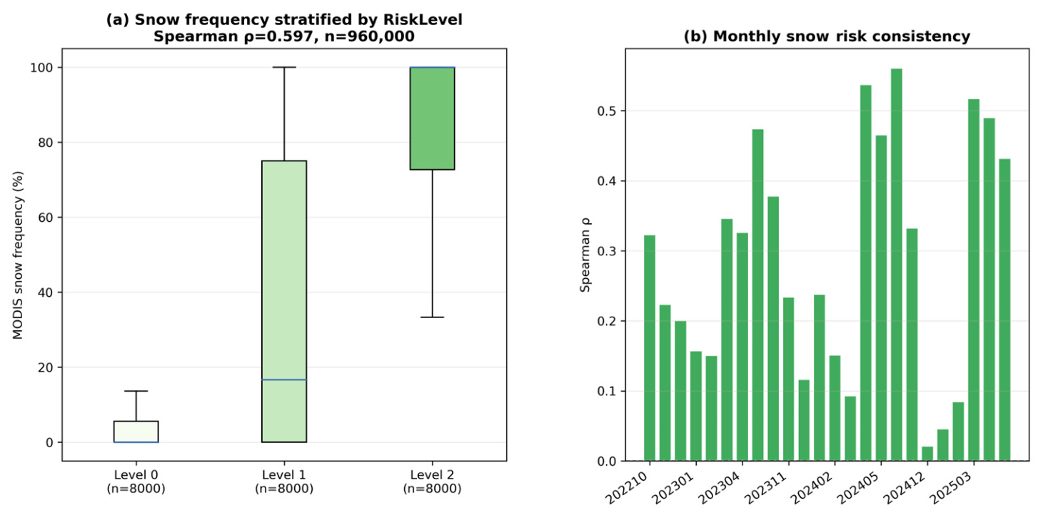
The monthly snow cover frequency (fraction of snow-covered days) was extracted from the MODIS snow cover product (NDSI ≥ 10) and used for spatial consistency testing against the RiskLevel. Since persistent snow cover provides the necessary moisture conditions for icing, a positive Spearman correlation coefficient ($\rho$) is expected between these two variables, thereby validating the model’s ability to characterize the moisture supply process.

Daily RiskLevel products were validated using Xinjiang transportation authorities’ operational road condition bulletins as independent ground truth. Icing risk validation was treated as a binary classification problem (1 = icing, 0 = no icing), limited to a 500 m buffer zone along G217, covering three 2022–2025 cold seasons. Spatiotemporally aligned 2 × 2 confusion matrices yielded verification metrics: POD, FAR, CSI, BIAS, ETS, and HSS. ETS and HSS were primary criteria to address icing’s imbalance and rarity, penalizing random hits and ensuring robustness. Note that a road condition bulletin does not guarantee no icing, possibly due to nighttime inspection gaps or low traffic.

2.4.7. Parameter Sensitivity and Uncertainty

A variance-based Sobol analysis quantified the influence of the risk integration parameters (the factor weights, the water availability threshold, and the penalty term). Saltelli samples were drawn within the ranges listed, and the response was the basin mean RiskScore over five representative winter dates spanning a range of cold, cloud, and precipitation conditions. Because these parameters act only in the final integration step, each sample was evaluated by re-scoring the pre-computed physical states. First-order ($S_1$) and total effect ($S_{\mathrm{T}}$) indices were then used to rank the parameters and to detect interactions.

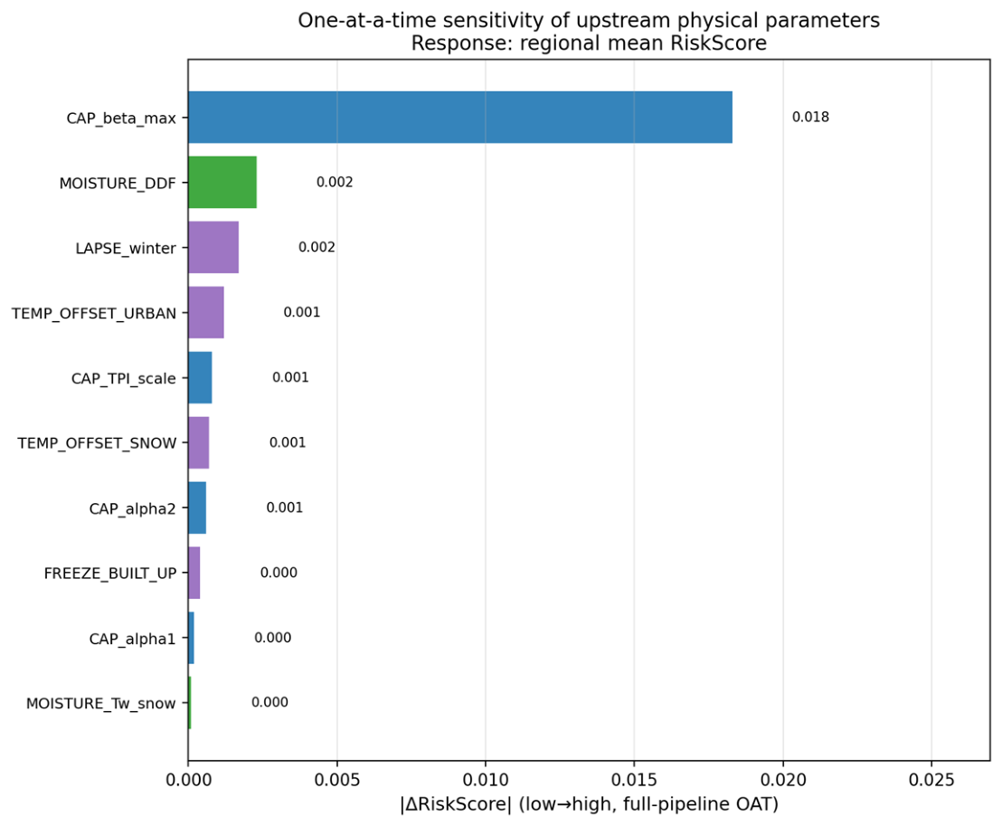
Parameters that set the upstream physical states—the lapse rate, the CAP cooling amplitude and terrain parameters, the degree-day factor, and the land cover temperature and freeze-point offsets—cannot be isolated by re-scoring. These were assessed with a full-pipeline one-at-a-time (OAT) analysis on two representative winter dates, in which each parameter, in turn, was set to the lower and upper bounds of its range while the others stayed at their defaults; sensitivity was taken as the absolute change in basin mean RiskScore between the two bounds.

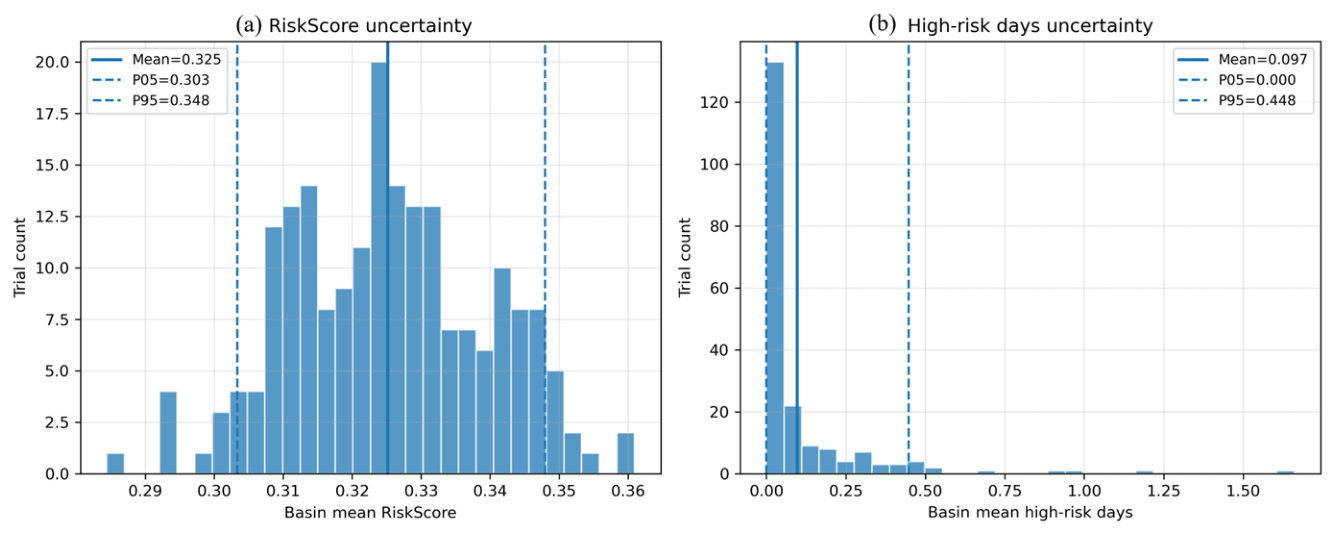
A Monte Carlo experiment then propagated the uncertainty in the most influential parameters into the final product. These parameters were perturbed by ±30% about their default values, and the full daily workflow was repeated over six representative icing-season dates for 200 realizations. Each realization produced a RiskScore map and a high-risk-day count, from which we derived the ensemble mean, standard deviation, and 5th, 50th, and 95th percentiles. These summaries characterized the uncertainty in the spatial pattern and the stability of the high-risk classification.

3. Results

3.1. Spatial Patterns of Terrain Factors

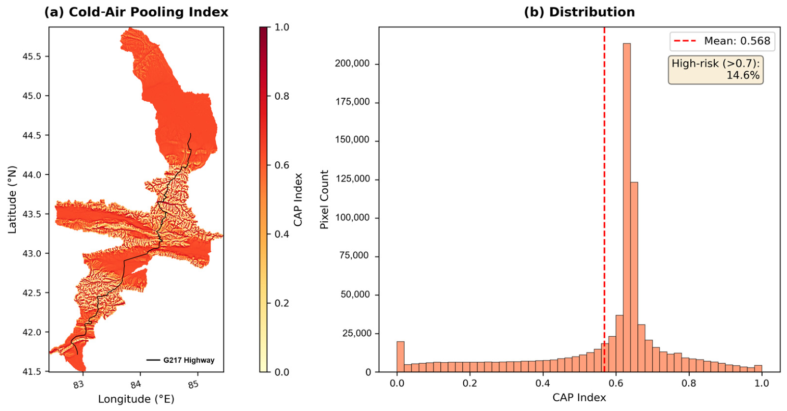
The DEM and its derived products revealed significant topographic heterogeneity in the study area, which exhibits extremely steep elevation gradients and pronounced geomorphic dissection, profoundly influencing local microclimates. The spatial distribution of the CAP index indicated that areas with high cold-air accumulation potential are mainly located at valley bottoms, gully confluence zones, and relatively enclosed low-lying terrain, consistent with the physical process of cold-air subsidence along slopes and convergence in topographic depressions (Figure 3a). High-risk cold pool zones (CAP > 0.7) accounted for 7.7% of the total basin area (Figure 3b) and were highly concentrated in enclosed deep valleys and basin bottoms, forming cold pool effect areas where extreme low temperatures occur frequently.

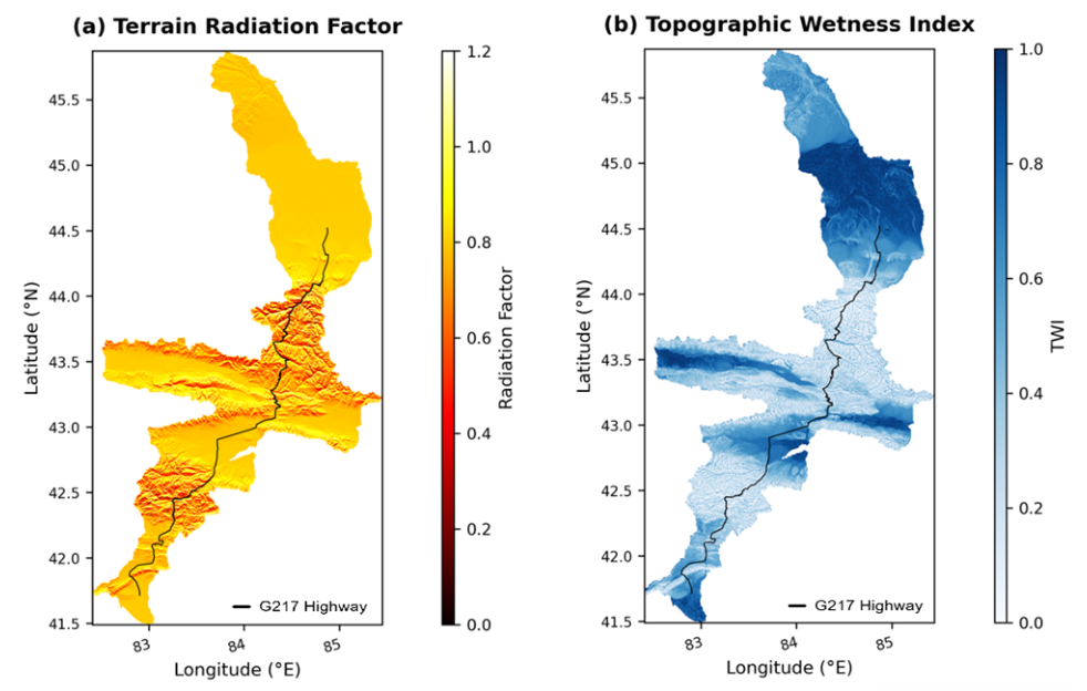
Topography also regulates the spatial redistribution of surface energy and moisture. Terrain radiation and TWI patterns show that shaded gullies and concave valley bottoms receive less potential radiation and tend to maintain higher surface wetness (Figure A1). The spatial overlap between radiation deficit, moisture convergence, and high CAP values provides favorable topographic conditions for near-surface icing in valley bottoms and road-adjacent low-lying corridors.

3.2. Temperature Field Reconstruction

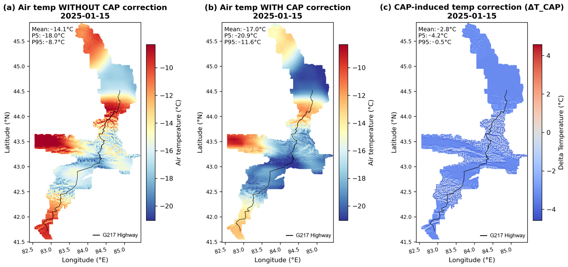
High-resolution, continuous LST is fundamental to accurate near-surface icing risk assessment. In the Tianshan study area, the downscaled air temperature field showed significant topographic modulation. Figure 4 presents ERA5 air temperature downscaling results and CAP correction differences. Baseline downscaling (Figure 4a) reasonably captured the macro-scale elevational temperature lapse rate. On 15 January 2025 (a representative cold-season day), the domain mean downscaled air temperature without CAP correction was −14.1 °C, showing pronounced elevational gradients and mountain–valley differentiation along the terrain and G217 corridor. After CAP correction (Figure 4b), near-surface air temperature decreased overall, with the regional mean dropping to −17.0 °C, reproducing micro-topographic temperature inversions. The CAP adjustment $\mathrm{\Delta }{T}_{CAP}$ was predominantly negative, with a mean correction of ~−2.8 °C and a 5–95% quantile range of −4.2 to −0.5 °C (Figure 4c). Valley bottoms and low-lying icing-prone areas had significant local cooling (up to 4–5 °C). CAP correction enhanced cooling signals in valleys, low-lying terrain, and road-adjacent topographically constrained zones, improving the spatial representation of near-surface freezing environments in complex mountains. Therefore, CAP provides physically meaningful terrain-resolved thermal information for subsequent icing-risk calculations. Without this correction, the temperature field would mainly follow background elevational gradients, and the local cold-pool effect in terrain-constrained regions would be significantly smoothed, potentially weakening the identification of valley-scale icing-prone areas.

The reconstruction accuracy of cloud-obscured LST and of the early morning minimum LST($T_{s,min}$) was quantitatively evaluated through a combination of internal cross-validation and independent comparison with Landsat LST. The monthly cross-validation results indicated that the reconstruction model achieved stable training accuracy throughout the cold season and captured the overall temperature variation well, with an overall cross-validated R² of 0.7821. Error differences among months were pronounced, demonstrating a marked seasonal dependence of temperature field reconstruction uncertainty. Errors were relatively small during stable, cold winter months but increased significantly during the spring snowmelt and rapid surface warming phase, with RMSE values rising to 23–35 °C in April and May. Monthly biases were mostly negative, indicating a systematic cold bias in the reconstructed $T_{s,min}$. This bias is related to the difference between the Landsat acquisition time and the time represented by $T_{s,min}$. The model was designed to provide a conservative minimum temperature constraint for freezing risk identification; consequently, this cold bias is acceptable for subsequent icing risk assessment.

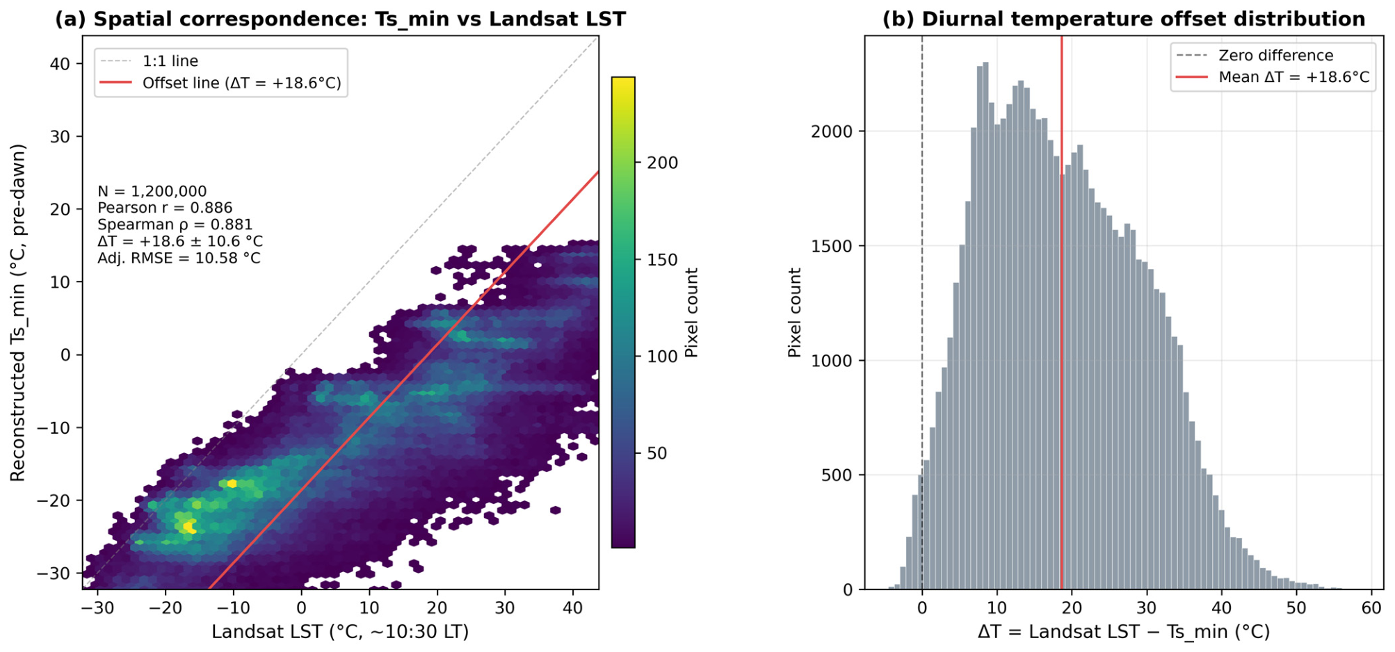
A pixel-wise comparison of the reconstructed $T_{s,min}$ with high-resolution Landsat clear-sky LST (Figure 5) was performed to evaluate the spatial consistency and absolute bias characteristics of the reconstructed temperature field. Figure 5 shows a high linear spatial correlation between the two (Pearson R = 0.886), indicating that the spatial pattern of the reconstructed temperature field is highly consistent with independent satellite observations and that the model preserves spatial temperature gradients and regional thermal state differences well. The reconstructed $T_{s,\mathrm{m}\mathrm{i}\mathrm{n}}$ lies on average about 18.6 °C below the coincident Landsat LST. This offset is not a reconstruction error but a consequence of comparing two different quantities: Landsat samples the surface during its mid-morning overpass, whereas $T_{s,\mathrm{m}\mathrm{i}\mathrm{n}}$is the nocturnal minimum. The clear-sky diurnal surface temperature range in this arid mountain region commonly exceeds 20–30 °C, and the offset varies accordingly, from roughly 9 °C in deep winter to roughly 30 °C in spring. The reconstructed minimum is therefore better evaluated against a nighttime reference: against the minimum air temperature at Bayanbulak (Section 3.5.4), the bias falls to −0.76 °C. We consequently use the Landsat comparison to verify the spatial pattern of the thermal field (Spearman ρ ≈ 0.88) and rely on the station minimum for absolute accuracy.

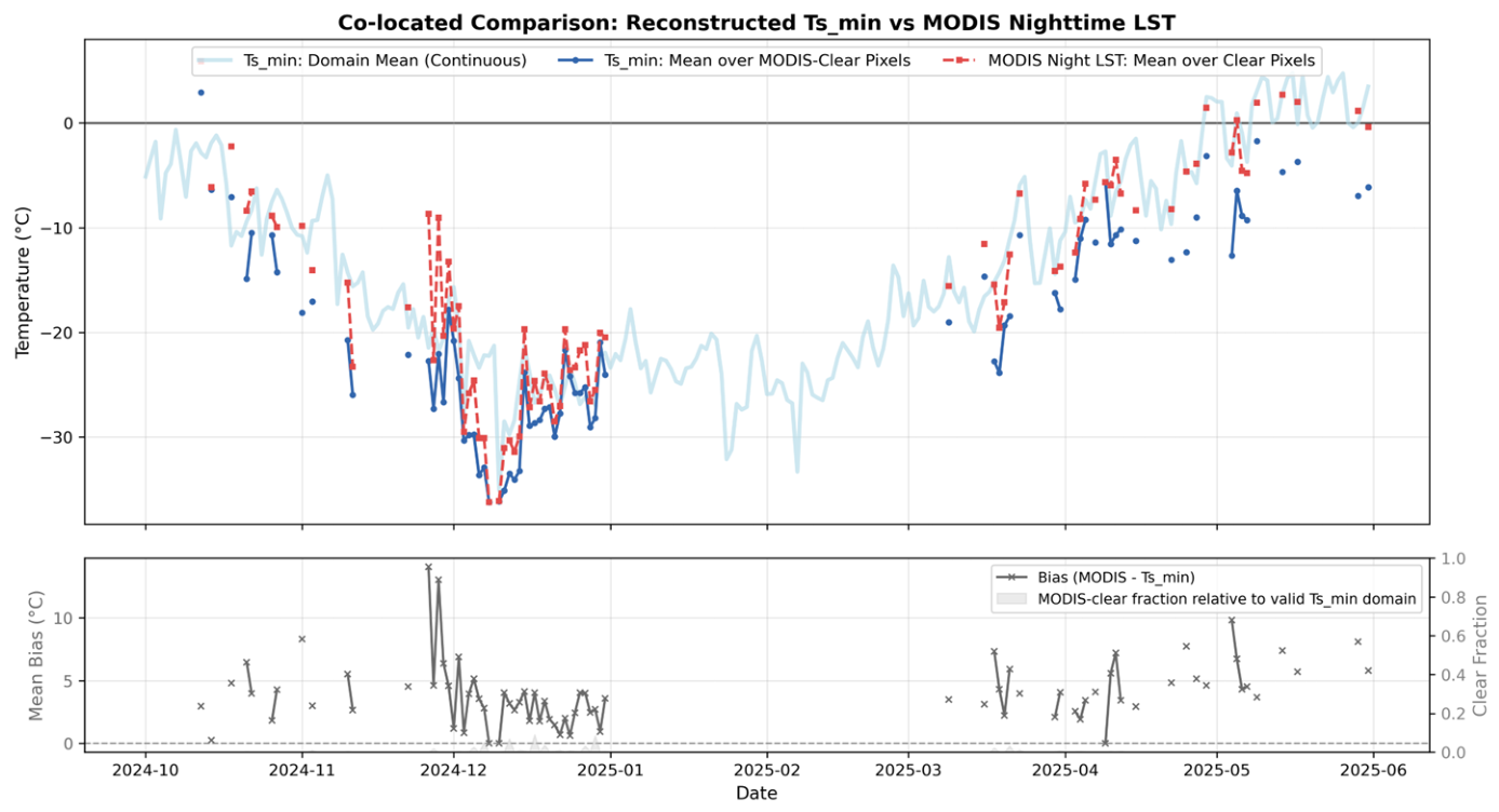
A co-located time-series comparison with MODIS nighttime clear-sky LST further supports the reconstruction framework (Figure A2). Reconstructed $T_{s,min}$ provides a continuous cold-season record, whereas MODIS nighttime LST is temporally discontinuous because of cloud contamination. The two series show consistent seasonal evolution, while MODIS nighttime LST is generally higher than $T_{s,min}$, consistent with the interpretation of $T_{s,min}$ as the daily minimum or near-minimum thermal state. This confirms that clear-sky MODIS observations alone are insufficient for continuous near-surface icing risk assessment.

3.3. Icing Risk Assessment Products

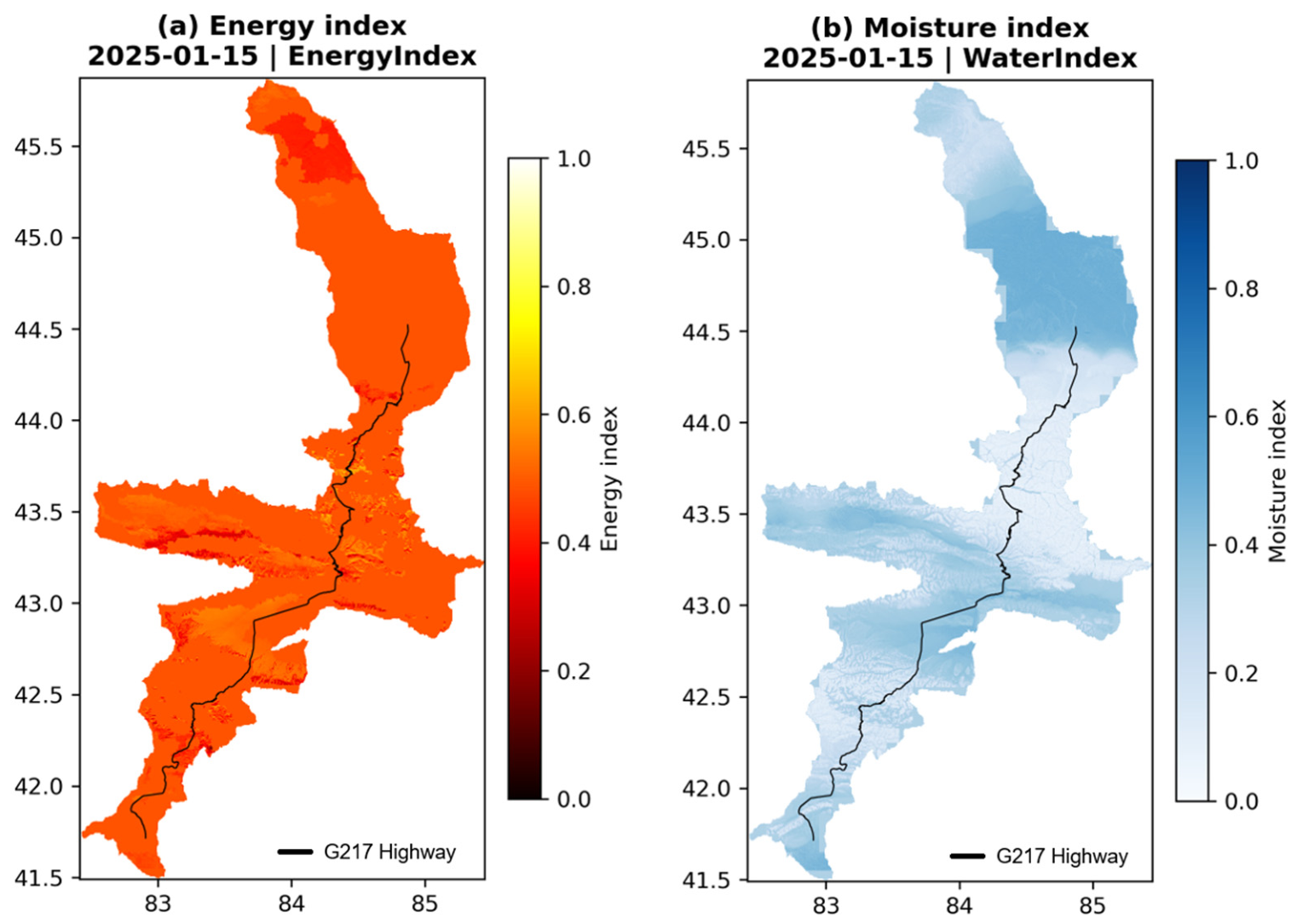
Based on energy constraints, moisture supply, freezing state, and topographic correction factors, a daily near-surface icing risk product was generated for the study area. The spatial patterns on typical days, cold-season temporal variations, monthly differences, high-risk zone distributions, and freezing rain potential hotspots were analyzed. The spatial pattern of icing risk is primarily determined by the heterogeneous distribution of energy and moisture. Taking a representative icing day (15 January 2025) as an example, the energy index (Figure 6a) exhibited local variations influenced by topography, slope aspect, and radiation conditions, decreasing significantly with increasing elevation and latitude, thereby reflecting the surplus cold energy required for freezing. In contrast, the moisture index (Figure 6b) showed more pronounced spatial differentiation, with relatively higher moisture conditions in the northern part of the study area and in some mountainous gully zones. Near-surface icing risk is not controlled solely by temperature but is jointly determined by the persistence of low temperatures and moisture availability. The energy index primarily characterizes the surface thermal and radiative background, whereas the moisture index reflects the material basis for icing, including precipitation, snow cover, meltwater, or a wet land surface.

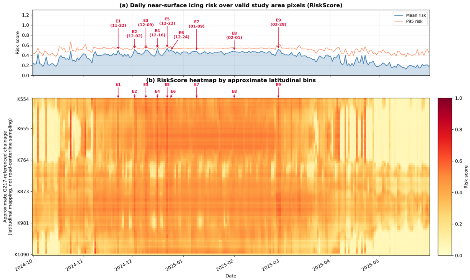
The daily risk time series revealed the phased evolution of icing risk throughout the cold season (Figure 7). Taking the period from October 2024 to May 2025 as an example, the area mean RiskScore gradually increased before winter, remained at a relatively high level from December to February, and then gradually decreased during the spring warming phase. The 95th percentile (P95) risk curve was generally higher than the mean risk, indicating the persistent presence of locally high-risk pixels within the study area during the cold season. The time series of mean risk and P95 risk clearly captured several typical acute icing events (labeled E1 to E9). Near these marked events, most corresponded to an increase in either mean risk or high-percentile risk (Figure 7a). These events coincided with extreme winter weather, demonstrating that the model captures the process of episodic risk elevation during the cold season. Figure 7b decomposes this temporal risk into a spatiotemporal heatmap along an approximate latitudinal station number (K-value) along the Duku Highway. The figure indicates that high-risk periods are not uniformly distributed along the route but are highly concentrated in specific elevation zones and latitudinal sections, particularly during December and January. It should be noted that the longitudinal K-values in Figure 7b are approximate zonal references and are not based on precise station numbers along the G217 highway centerline; therefore, this figure is primarily intended to illustrate the spatiotemporal differentiation of risk within the study area rather than risk localization at the highway centerline level.

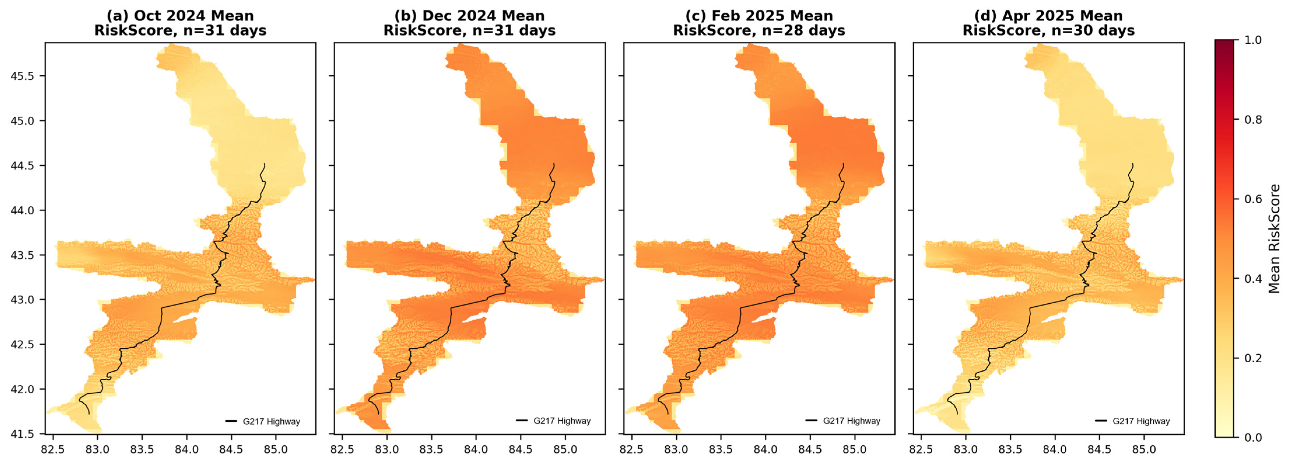
The monthly mean risk distribution exhibited clear seasonal evolution characteristics (Figure 8). In October 2024, the overall risk in the study area was low to moderate, indicating that low-temperature conditions had not yet fully stabilized in the early cold season. During the deep winter months, extensive high-risk areas appeared in the north-central part of the study area. Risk increased markedly in December, particularly in mountainous gullies, slopes, and areas near roads, and remained at a relatively high level through February of the following year, indicating that freezing conditions and moisture availability continued to support icing risk formation in the middle to late winter. As air temperatures rose and the conditions sustaining freezing weakened, the overall mean risk decreased by April. This inter-monthly variation is consistent with the temperature field reconstruction results and the seasonal variation in cold-season moisture conditions, demonstrating that the model captures the progression of near-surface icing risk from formation and maintenance in the cold season to attenuation in spring.

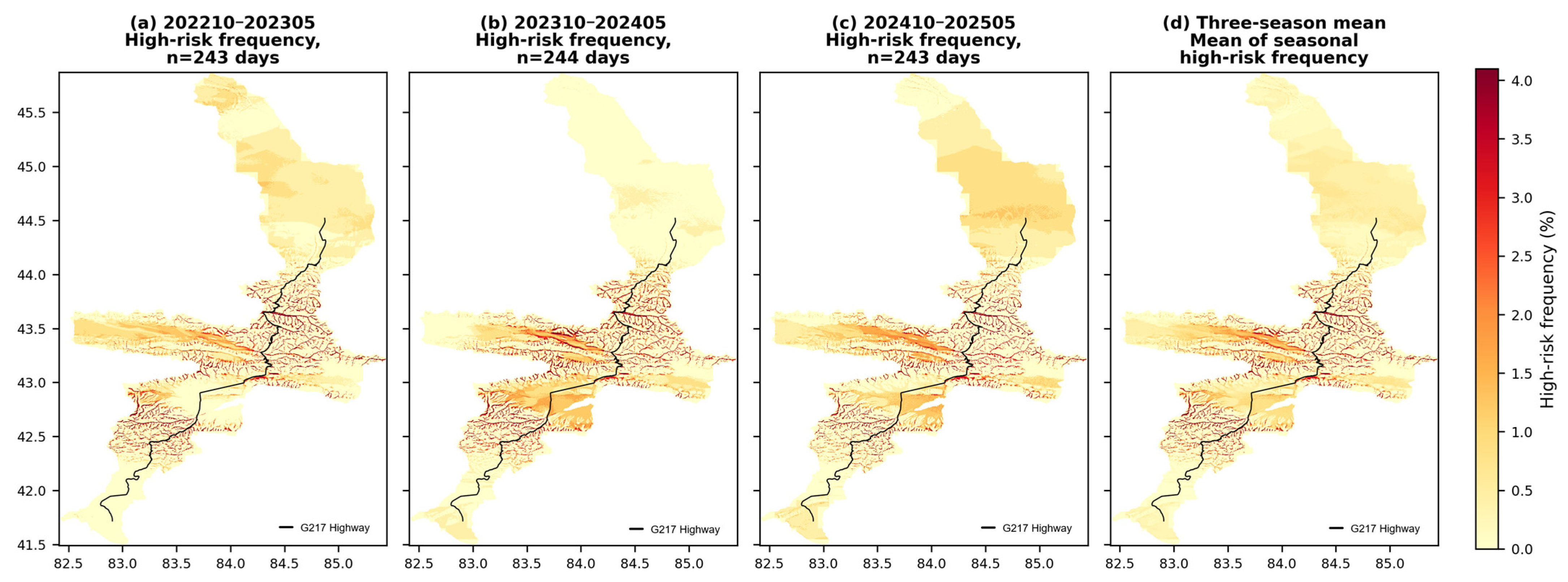
For practical icing hazard assessment, identifying persistent high-risk corridors is essential. The inter-annual high-risk frequency, defined as the percentage of days with RiskLevel ≥ 3, highlights the spatial concentration of persistent risk along central mountainous gullies, slope convergence zones, and selected sections of the G217 corridor (Figure 9a–c). High-risk events are generally short-lived, indicating that severe near-surface icing is episodic and patchily distributed. The three-season mean (Figure 9d) indicates that these high-risk zones are spatially persistent, while the year-by-year panels also reveal clear inter-annual differences: the 2024–2025 season shows higher high-risk frequency in the G217 valleys, possibly related to inter-annual differences in cold-air activity and precipitation conditions.

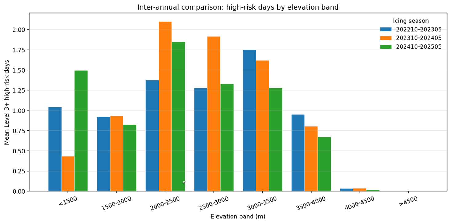
The elevation band analysis further shows that Level 3+ high-risk days were not uniformly distributed with elevation (Figure 10). Across the three icing seasons, the highest values generally occurred in the 2000–3500 m elevation range, while the >4000 m bands had very few Level 3+ high-risk days. This pattern is physically consistent with the combined effect of sufficiently low temperature, available moisture, valley-scale cold-air pooling, and snowmelt–refreezing conditions. At the highest elevations, temperature conditions are frequently favorable for freezing, but moisture availability and persistent snow/ice cover reduce the frequency of near-surface icing conditions as defined by the risk index. Inter-annual differences were also evident. The 2023–2024 and 2024–2025 seasons showed higher Level 3+ high-risk-day counts in the 2000–3000 m bands than 2022–2023, whereas the 3000–3500 m band was more prominent in 2022–2023. Low-elevation risk also varied substantially among years. These differences show that the three-season mean should be interpreted as a summary of the study period, not as a fixed climatological pattern. Nevertheless, the repeated concentration of high-risk days in the 2000–3500 m corridor supports the robustness of the main elevation-dependent conclusion over the three independent icing seasons.

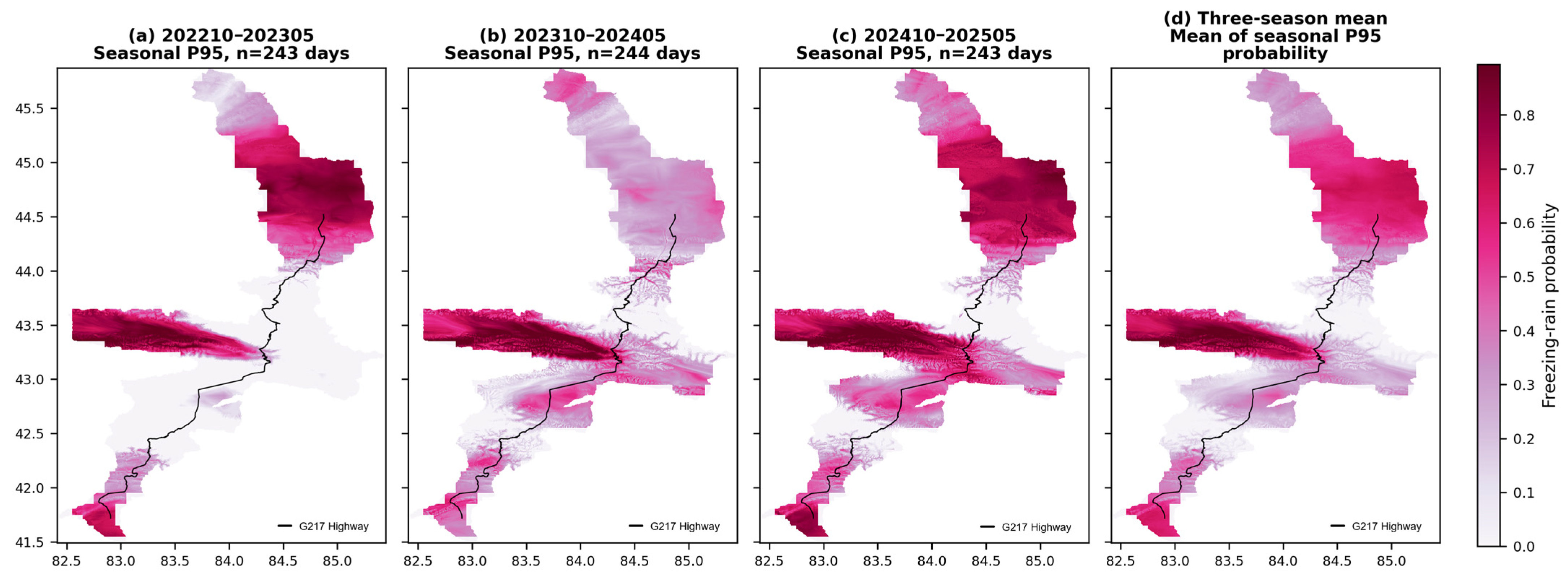
Freezing rain potential, represented by the seasonal 95th percentile of $P_{fr}$ (Figure A3), exhibits a distinct spatial pattern, with high values mainly in northern and eastern areas and some west-facing mountain branches. These zones are prone to freezing rain formation where low temperatures coincide with sufficient moisture. However, high $P_{fr}$ does not necessarily correspond to Level 3+ RiskLevel zones (Figure 9). This is because RiskLevel requires simultaneous satisfaction of multiple factors—temperature, moisture, energy deficit, terrain effects, and hard constraints—so areas with high $P_{fr}$but weaker conditions in other factors may not reach persistent high-risk classification. This comparison highlights the different physical meanings of the two products. RiskLevel identifies locations where multiple icing-favoring processes overlap, suitable for locating persistent near-surface icing corridors. In contrast, $P_{fr}$ isolates precipitation-phase-specific hazards and should be interpreted as complementary information. The spatial discrepancy between Figure 9 and Figure A3 is thus physically meaningful, reflecting the conditional role of freezing rain within the integrated risk framework rather than underestimation by the ${\beta }_5$ weight.

3.4. Cold-Season Cumulative Statistics Products

To reduce the influence of single-year meteorological anomalies on cold-season statistics, the study employed daily minimum surface temperature ($T_{s,min}$) and RiskLevel products from three consecutive cold seasons (2022–2023, 2023–2024, and 2024–2025). Freezing degree days (FDD), melting degree days (MDD), freeze–thaw cycles (FTCs), and high-risk days were all computed within each cold season separately, and the multi-year averages were then derived from these seasonal values. Computing FDD, MDD, and FTCs independently within individual cold seasons avoids spurious freeze–thaw transitions that would otherwise appear across cold-season boundaries.

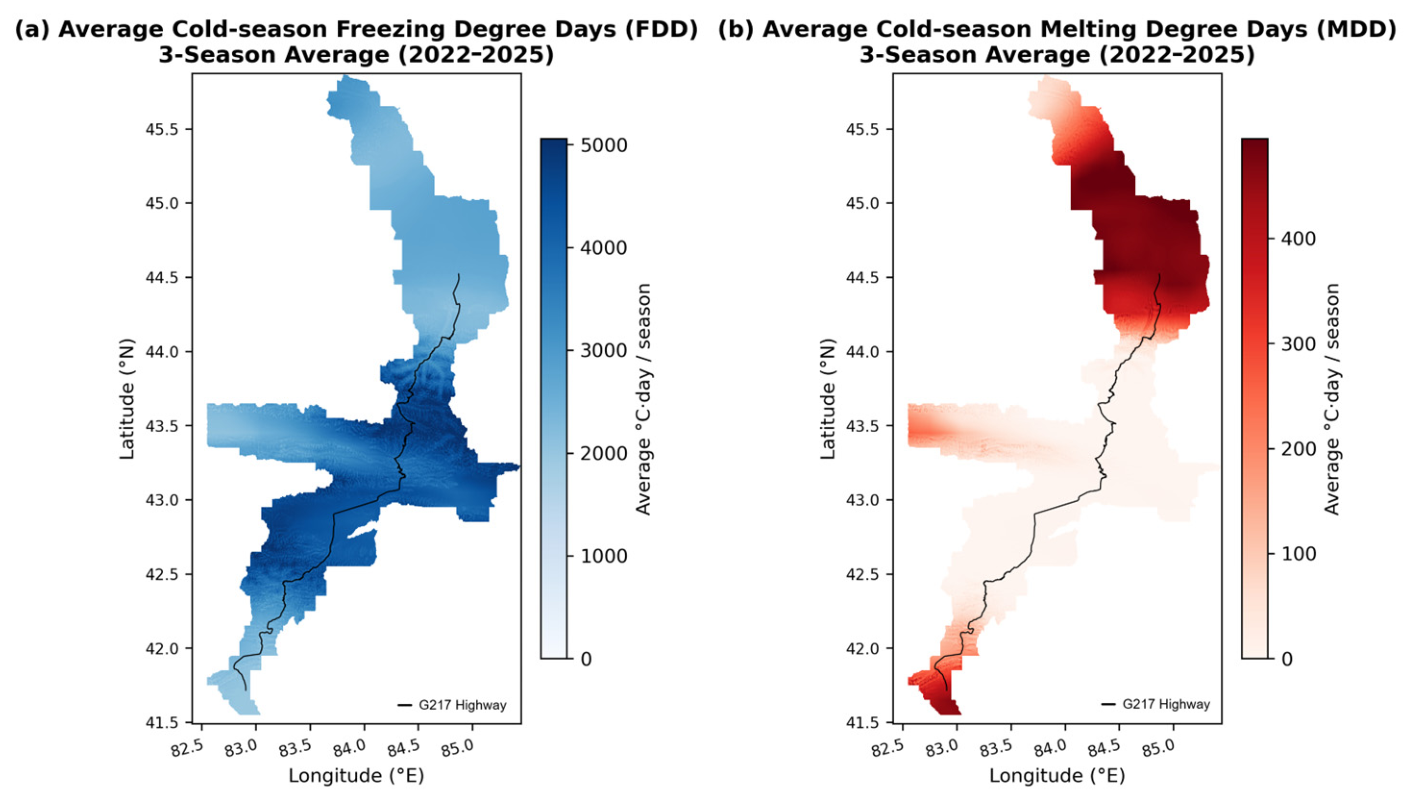
Cold-season FDD displayed a clear topographic differentiation across the study area (Figure 11). The highest FDD values occurred in mid- to high-elevation mountains, headwater gullies, and zones of strong topographic relief, pointing to enhanced cold-air accumulation and sustained freezing throughout the cold season. MDD primarily clustered in low-elevation, relatively warm and humid areas. MDD values dropped steeply with elevation and approached zero above 2000 m, indicating that high-elevation sites rarely record daily minimum temperatures above 0 °C during the cold season. FDD and MDD showed contrasting spatial patterns, reflecting a cold-season thermal regime shaped jointly by elevation, topography, and local cold-air pooling.

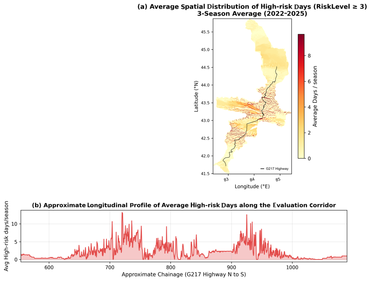
Defining RiskLevel ≥ 3 as a high-risk condition, the distribution of high-risk days was strongly localized (Figure 12a). High-risk days clustered in mountainous gullies in the central mountain gullies, on hillslope convergence zones, and along topographically constrained road sections associated with the G217 corridor, all within the study area. Across most of the study area, high-risk days remained sparse, indicating that high-risk conditions tend to be short-lived and event-driven, emerging from specific conjunctions of low-temperature, moisture, and freeze–thaw conditions. In certain topographically complex zones, however, hazardous conditions persisted over longer periods. A longitudinal profile along the G217 evaluation corridor (Figure 12b) demonstrated that risk along the road is not uniformly distributed but is instead modulated by topographic channeling, elevation gradients, and local hydrothermal conditions. Multiple “risk hotspots” were identified between approximately chainages K800 and K980, with high-risk days exhibiting pronounced peaks in several segments. Several road sections recorded more than 10 high-risk days, and multiple peaks in the profile coincided with high-elevation passes where moisture convergence and subfreezing temperatures frequently occur together.

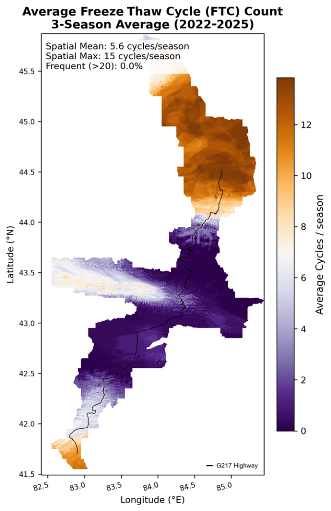
Freeze–thaw cycles (FTCs) indicate how frequently the reconstructed $T_{s,\mathrm{m}\mathrm{i}\mathrm{n}}$ fluctuates around 0 °C, capturing active near-surface ice–water transitions (Figure A4). High FTC values mainly occur in low-elevation and thermally transitional areas, while mid- to high-elevation zones remain continuously frozen. This spatial pattern highlights where repeated freeze–thaw transitions may contribute to icing events, complementing RiskScore and RiskLevel assessments. Cold-season metrics stratified by elevation (

Table 4. Three-season average elevation-band statistics of FDD, MDD, FTCs and high-risk days.

Elevation Band	N Pixels	Area (km2)	Avg FDD (°C·d/Season)	Avg MDD (°C·d/Season)	Avg FTC (Cycles/Season)	Avg High-Risk Days/Season
<1000 m	233,969	14,623.1	2538.9	401.3	11.7	1.2
1000–2000 m	164,143	10,258.9	2750.3	149.7	6.6	1
2000–3000 m	200,126	12,507.9	4084.6	9	1.5	1.6
3000–4000 m	143,286	8955.4	4480.8	1.6	0.5	1.4
>4000 m	6081	380.1	4784.7	0.1	0.1	0

) showed a steady rise in FDD with elevation, from 2538.9 °C · d season⁻¹ below 1000 m to 4784.7 °C · d season⁻¹ above 4000 m. MDD followed the reverse pattern, dropping sharply from 401.3 °C · d season⁻¹ in the lowest elevation band to 0.1 °C · d season⁻¹ above 4000 m. FTCs also rose markedly with decreasing elevation, indicating more frequent freeze–thaw transitions in low-elevation areas. The mean number of high-risk days peaked at 1.6 days season⁻¹ within the 2000–3000 m elevation band. The risk of near-surface icing is shaped jointly by freezing conditions, moisture availability, and freeze–thaw transitions, rather than by low temperature intensity alone.

3.5. Validation Results

The reconstructed icing risk product was validated from multiple independent perspectives, including LST reconstruction accuracy, spatial consistency against high-resolution Landsat observations, agreement with MODIS snow cover frequency, comparison with a high-altitude independent station, and reported icing events in traffic bulletins.

3.5.1. Reconstruction Accuracy and Feature Contribution

Across twelve anchor days, the number of cloud-free training pixels ranged from ~500 to 470,000, reflecting strong daily variation in clear-sky coverage. Convergence tests indicated that the spatially cross-validated RMSE plateaued near 1.9 K once ~50,000 pixels were used, justifying a daily training cap. Spatial block cross-validation yielded RMSE ≈ 2.0 K, lower than random five-fold CV (RMSE ≈ 1.2 K) due to spatial autocorrelation. The ensemble stacking model reached RMSE = 1.90 K, MAE = 1.29 K, and R² = 0.99. Permutation importance showed ERA5-Land thermal fields dominated (ΔRMSE ≈ 0.64 K), followed by elevation (≈0.26 K) and day-of-year cosine (≈0.13 K), with terrain and land cover variables contributing marginally, consistent with the expected physical controls.

3.5.2. Spatial Consistency with Landsat LST

Although the inclusion of Landsat-9 increased the observation frequency, Landsat remains constrained by its revisit cycle and clear-sky requirement. Therefore, it does not substantially alleviate short-term cloud contamination relative to MODIS. Here, Landsat was used mainly as an independent high-resolution reference to assess the spatial consistency and fine-scale temperature patterns of the reconstructed LST product. The reconstructed pre-dawn minimum land surface temperature ($T_{s,min}$) was compared with independent Landsat 8/9 Collection 2 Level-2 thermal infrared observations across 24 cold-season months, with 1.2 million pixel level validation pairs (Figure 5a and Figure 13). A Pearson r of 0.886 and a Spearman ρ of 0.881 pointed to a close spatial correspondence between the reconstructed and observed LST fields. Because $T_{s,min}$ captures the pre-dawn minimum and Landsat overpasses occur near 10:30 local time, a systematic temperature difference is physically expected. The mean diurnal temperature difference ΔT across all months was +18.6 °C. Winter values (December to January) hovered near +9.0 °C, while the spring transition (April to May) saw offsets of about +30.0 °C. Stronger daytime solar radiation drives a larger diurnal cycle, as expected from the surface energy balance climatology of continental mountain environments (Figure 5b). After removing this diurnal offset, the residual RMSE was 10.58 °C. Spatial correlations remained moderate to high in most months, while the temperature offset and RMSE showed clear seasonal differences (Figure 13). Comparisons with Landsat data suggest that the reconstructed temperature field captures spatial thermal gradients effectively.

3.5.3. Consistency with MODIS Snow Cover Frequency

Validation against MODIS snow frequency confirmed strong agreement between model-identified high-risk areas and snow or moisture presence. MODIS snow frequency and RiskLevel exhibited a mean Spearman ρ of 0.597 (N = 960,000) (Figure 14). Pixels with higher RiskLevels consistently corresponded to higher snow frequencies. Model-identified high-risk areas typically had greater snow cover or moisture availability, consistent with the physical requirement that near-surface icing depends on both low temperatures and available moisture. The correlation peaked in early autumn (October to November, ρ = 0.50–0.56) and late spring (April to May, ρ = 0.45–0.57), when the spatial contrast between snow-covered and snow-free surfaces was most pronounced (Figure 14b). Snow frequency in RiskLevel 2 areas was consistently and significantly higher than in RiskLevel 0 areas (Figure 14a), confirming that the model’s moisture supply component correctly identifies persistently snow-covered areas as zones of high icing risk.

3.5.4. Validation Against High-Altitude Station

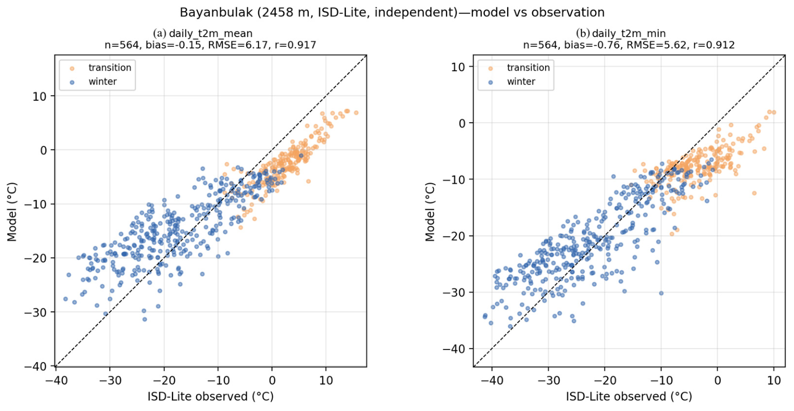
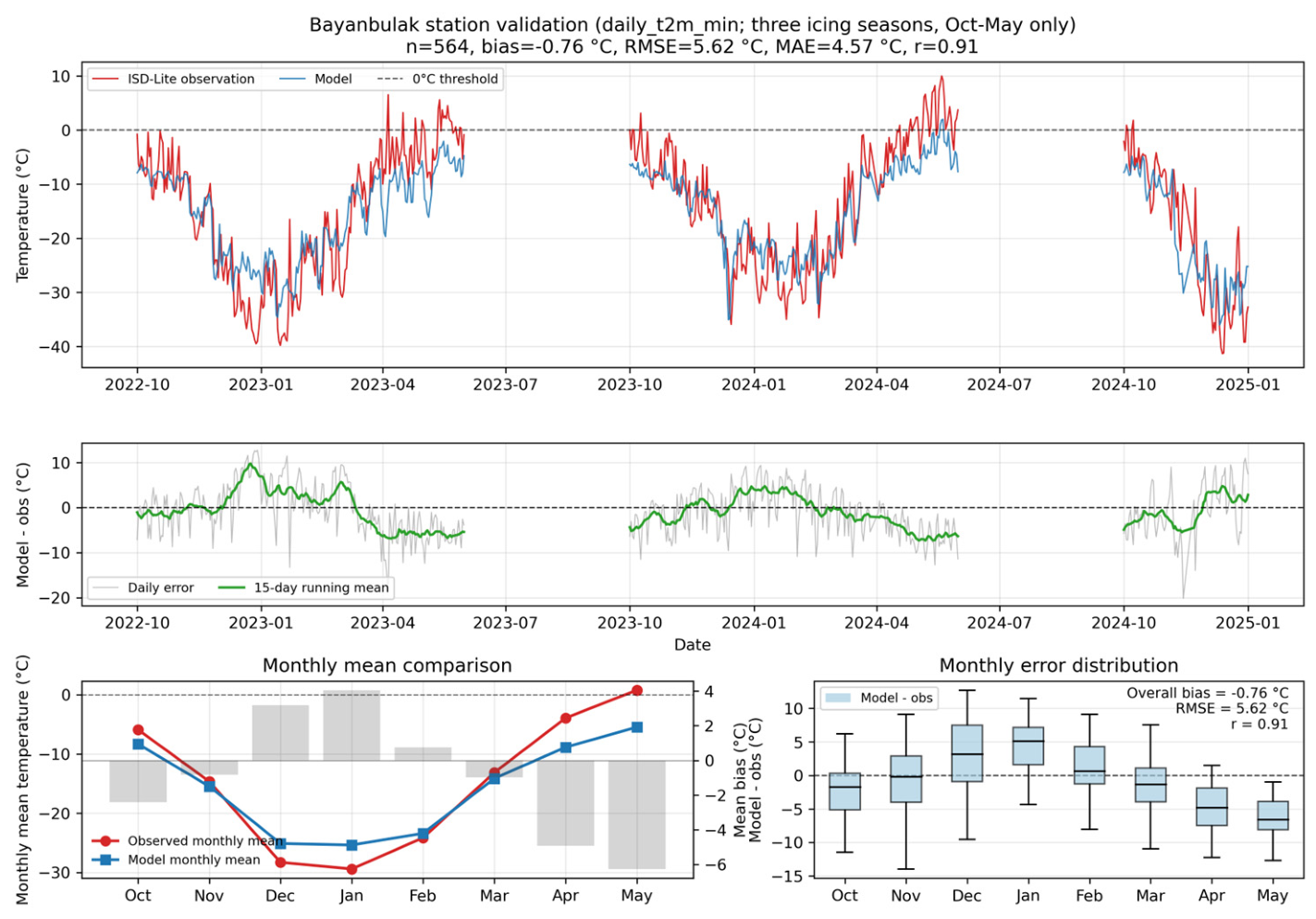
The reconstructed near-surface air temperature was compared with daily records from the Bayanbulak station (ISD-USAF 515420, 2458 m a.s.l.) on the G217 corridor. This station-based comparison provides an independent evaluation of the atmospheric thermal component used in the icing risk framework, rather than a direct validation of the reconstructed LST itself. Landsat LST is instead used to evaluate the spatial consistency of reconstructed surface thermal patterns because Landsat represents mid-morning surface temperature rather than the nocturnal minimum thermal state. These records come from the NOAA Integrated Surface Database (ISD-Lite) and were not used for model training or parameter calibration, so the comparison provides an independent ground-based check at the high elevations that dominate the corridor and are poorly sampled by valley stations. The matched record spans three icing seasons (2022–2025). The station archive ends on 1 January 2025, so the third season is represented only by its early part (October–December 2024); the matched sample totals 564 station-days. For the daily minimum temperature, which governs the icing diagnosis, the model matched the station with a mean bias of −0.76 °C, an RMSE of 5.62 °C, an MAE of 4.57 °C and a correlation of r = 0.91; the daily mean temperature gave a bias of −0.15 °C, an RMSE of 6.17 °C and r = 0.92 (Figure 15). The reconstruction reproduces the observed seasonal cycle and the day-to-day variation at the site, and the overall bias is stable across the three seasons, with a seasonal minimum temperature bias between −0.4 and −1.3 °C. Station validation confirms the physical plausibility of the temperature field but does not directly confirm the absolute accuracy of the reconstructed LST.

The near-zero overall bias conceals an offset that changes sign with season (Figure 16). In mid-winter, the model is slightly warm (minimum temperature bias +1.3 °C), which is consistent with the station lying in a cold-pooling basin, whose most extreme nighttime cooling a coarse reconstruction only partly resolves. In the transition months the model is several degrees too cold (bias −4.2 °C) and less well correlated (r = 0.63). The transition-season cold bias matters more for the icing diagnosis because it falls in the period when temperatures sit near 0 °C and the freezing threshold is in play. In those months the reconstruction will tend to over-identify near-freezing conditions rather than miss them, which is the conservative direction for a screening product. A third point concerns record length. Because the station data end on 1 January 2025, the 2024–2025 season contributes only 86 of the 564 station-days, against 240 and 238 for the two complete seasons, and the spring transition of 2025 is not sampled. The transition-season statistics therefore rest mainly on the two earlier seasons.

3.5.5. Event-Level Evaluation Against Traffic Bulletins

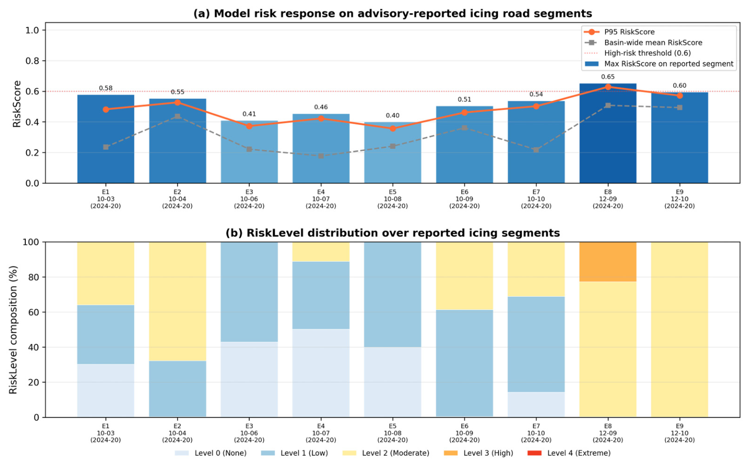
Validation against icing events documented in traffic bulletins was used to evaluate the correspondence between modeled risk and reported affected road sections. A multi-threshold analysis on nine effective event days showed that the highest Equitable Threat Score was obtained when RiskLevel ≥ 2 was used as the warning threshold (Figure 17a). At this threshold, the model yielded a Probability of Detection (POD) of 0.485, a False Alarm Ratio (FAR) of 0.682, a Critical Success Index (CSI) of 0.238, an Equitable Threat Score (ETS) of 0.035, and a frequency bias of 1.52. These values indicate limited event-level predictive skill when the framework is evaluated as a daily discrete event detector against traffic bulletin records. The high FAR and frequency bias greater than 1 show that the model identifies a broader high-risk area than the bulletin-confirmed icing extent. This overprediction should not be interpreted as operational reliability. Several factors may contribute to the low event-level scores. First, traffic bulletins usually describe events by road segment, mileage marker, or nearby settlement, whereas the model output is evaluated on a 250 m grid; this spatial mismatch can inflate both false alarms and misses. Second, reported events often correspond to traffic disruption or observed driving conditions, while the model partly represents daily minimum thermal conditions, which may introduce a 6–12 h temporal mismatch. Third, road-specific processes, including pavement material, de-icing operations, traffic-induced heat, drainage conditions, local shading, and maintenance activities, are not explicitly represented in the current framework. Finally, traffic bulletins are incomplete as physical icing observations because they mainly record reported incidents or disruptions; icing-prone conditions without reported accidents may be absent from the event inventory. Nevertheless, the modeled RiskScore along the reported road segments was generally higher than the basin-wide mean. For the nine event days, the maximum RiskScore along reported road sections ranged from 0.40 to 0.65. Winter events (E8–E9, December 2024) approached the high-risk threshold (0.60–0.65), whereas transitional events (E1–E7, October 2024) mostly fell between 0.40 and 0.55. Both the maximum and 95th-percentile RiskScore values for bulletin events were higher than the basin-wide mean (gray dashed line in Figure 17a), with enhancement factors of approximately 1.5–2.5. This suggests that the framework captures a relative spatial risk signal for some reported icing sections, although it does not provide stable high-risk classification for all events. The RiskLevel breakdown further shows that reported icing sections were mainly classified as Levels 1–2, with only some winter events reaching Level 3. Therefore, the current product should not be regarded as a deterministic predictor of reported road icing events. Its appropriate use is as a spatially continuous, physically interpretable screening layer for identifying potentially icing-prone road corridors at the sub-kilometer scale. It should complement, rather than replace, road weather stations, pavement sensors, visual monitoring, traffic bulletins, and operational short-range forecasts. The limited number of traffic bulletin events provides illustrative evidence of screening-level capability; absolute skill metrics remain low, and FAR is high.

3.6. Parameter Sensitivity and Uncertainty Results

3.6.1. Sobol Sensitivity of Risk Integration Parameters

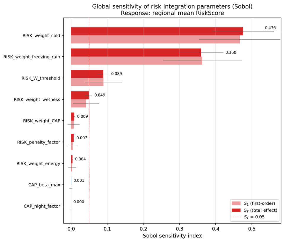
Sobol analysis showed that a few risk integration parameters controlled the RiskScore (Figure A5;

Table 5. Sobol sensitivity indices of risk integration parameters.

Parameter	Default	Range	${\mathit{S}}_1$	${\mathit{S}}_{\mathbf{T}}$	Rank
weight_cold	0.25	0.15–0.40	0.47	0.48	1
weight_freezing_rain	0.2	0.10–0.30	0.36	0.36	2
W_threshold	0.1	0.05–0.20	0.09	0.09	3
weight_wetness	0.25	0.15–0.40	0.04	0.05	4
weight_CAP	0.15	0.05–0.25	0.009	0.009	5
penalty_factor	0.3	0.10–0.50	0.007	0.007	6
weight_energy	0.15	0.05–0.25	0.004	0.004	7
${\beta }_{CAP}$	5	2.0–7.0	<0.001	0.001	8
night_factor	1	0.7–1.3	<0.001	<0.001	9

Note: Indices computed with N = 256 (2816 model evaluations) over five deep-winter dates. For the lowest-ranked parameters, S₁ and S_T coincide within Monte Carlo error; the first-order indices sum to ≈ 0.97, confirming a near-additive response.

). The low-temperature weight dominated ($S_{\mathrm{T}}$ = 0.476), with the freezing rain weight second ($S_{\mathrm{T}}$ = 0.360) and the water availability threshold third ($S_{\mathrm{T}}$ = 0.089); every other parameter contributed less than 0.050. First-order and total effect indices nearly coincided, and the first-order indices summed to about 0.970, so the integration layer was effectively additive with negligible interactions. A leading role for the low-temperature weight is expected since near-surface icing is governed primarily by freezing conditions. The high rank of the freezing rain weight needs context. The deep-winter dates used here carried near-zero freezing rain probability, so perturbing this weight changed the RiskScore mainly by renormalizing the active factors rather than through a freezing rain signal. Its direct effect should emerge in transition seasons, when freezing rain is more likely.

3.6.2. OAT Sensitivity of Upstream Physical Parameters

The full-pipeline OAT analysis gave small absolute responses for all upstream physical parameters (Figure 18). The maximum cold-pool amplitude ${\mathrm{\beta }}_{CAP}$ ranked first, yet varying it across 2–7 °C shifted the basin mean RiskScore by only about 0.018, roughly 3.7% of the basin mean on the two evaluation days. The degree-day factor and the winter background lapse rate followed at about 0.002, and the rest—the CAP weights ${\mathrm{\alpha }}_{TPI}$ and ${\mathrm{\alpha }}_{Z_{rel}}$, the TPI normalisation scale, and the land cover temperature and freeze-point offsets—stayed at or below 0.001, with the CAP weights essentially inert (|ΔRiskScore| ≈ 0.0002–0.0006). The upstream modules therefore carry many empirical constants but move the regional RiskScore far less than the integration weights do, so the main conclusions do not hinge on their exact values.

3.6.3. Monte Carlo Uncertainty Propagation

Monte Carlo propagation indicated a stable regional magnitude (Figure 19a). Across 200 realizations, the basin mean RiskScore was 0.33, with a 5th–95th percentile range of 0.30–0.35 (about ±7%), so the overall level held under reasonable perturbation of the most influential parameters. The basin mean high-risk-day count was far less certain in relative terms (mean 0.10; 5th–95th percentiles 0.00–0.45; Figure 19b), as expected for a threshold metric with a low base rate over the short evaluation window. We therefore report the high-risk-day count as a limitation of threshold-based reading rather than as instability of the continuous risk field.

3.6.4. Physical Interpretability and Factor Decomposition

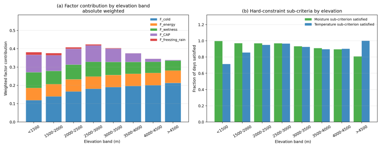
We decomposed the RiskScore at each pixel and day into its five weighted factor contributions—cold, energy, wetness, CAP, and freezing rain—and aggregated them by elevation (Figure 20a). The pattern is physically coherent. The low-temperature term carries most of the score at every elevation and grows toward the colder, higher bands. The cold-air-pool term is concentrated in the low-to-mid-elevation valleys and becomes negligible above about 4000 m, while freezing rain appears only in the lowest, warmest bands. Each high-risk pixel can therefore be traced to a dominant physical driver rather than read as a single composite number. The hard-constraint sub-criteria explain the elevation trend further (Figure 20b). At low elevations, the temperature criterion is the more frequent limiter; higher up, it is almost always satisfied, and moisture availability becomes the limiting term, which is why the high-risk frequency falls toward the highest bands.

4. Discussion

Near-surface icing risk in complex mountainous regions is controlled not only by large-scale cold-air processes but also by local topography. Mountain valleys, footslopes, and low-lying corridors are prone to cold-air accumulation under nocturnal radiative cooling, weak winds, and stable stratification, leading to locally lower near-surface temperatures than adjacent slopes at similar elevations. This pattern is consistent with previous studies on mountain microclimate, cold-air pooling, and valley inversions, which show that valleys and terrain-constrained corridors can cool more strongly at night than adjacent slopes. In this study, the CAP correction enhances these low-temperature signals in valleys and low-lying corridors and reduces smoothing errors from coarse-resolution reanalysis data such as ERA5-Land. Elevation band statistics further show that high-risk days do not increase monotonically with elevation but are concentrated mainly in the 2000–3000 m band and, to a lesser extent, the 3000–4000 m band. This differs from simple lapse-rate-based interpretations, in which the coldest and highest elevations would be expected to show the greatest risk. A likely explanation is the joint control of temperature and moisture: above approximately 3500 m, freezing conditions are common, but liquid water availability and melt–refreeze transitions are limited. Therefore, near-surface icing risk is best understood as the combined outcome of low temperature, moisture availability, freeze–thaw transitions, and terrain-induced cold-air pooling, rather than as a simple function of elevation alone.

Existing icing monitoring and warning methods mainly include single-meteorological-threshold approaches, statistical empirical models, road weather station monitoring, and numerical-forecast-driven models. Single temperature thresholds are simple and easy to implement operationally, but they cannot distinguish among different icing-related scenarios, such as dry-cold conditions, wet-cold conditions, snow cover, and snowmelt refreezing. Statistical models can establish empirical relationships from historical events, but they depend strongly on training samples, and their spatial generalization is limited in mountainous areas where stations are sparse and event records are incomplete. Road weather stations and pavement sensors can directly characterize road surface conditions, but their density is often insufficient in mountain corridors, making it difficult to support continuous spatial mapping. Compared with these existing methods, the framework proposed in this study should be regarded as a complementary approach rather than a replacement. Its main advantage is the spatially continuous representation of icing-prone terrain by integrating all-weather thermal reconstruction, moisture constraints, terrain effects, and cold-air-pooling correction. This allows the framework to serve as a screening-level risk-mapping layer for identifying potentially hazardous road segments between monitoring points. At the same time, its application boundaries should be clearly recognized. The product is neither a deterministic observation of road surface conditions nor an operational event forecast. It remains affected by uncertainties associated with land surface temperature reconstruction, temperature downscaling, parameter selection, and limited ground validation. For practical winter road management, this framework should therefore be used together with road weather stations, pavement sensors, vision-based recognition, and short-range numerical forecasts.

The proposed framework captures several conditions favorable for icing, including low temperatures, moisture availability, terrain-induced cold-air pooling, and a negative surface energy balance. Daytime melting followed by nighttime refreezing may contribute to black ice formation during transition periods, but this mechanism was not directly quantified in this study. Specifically, melt-day and refreezing-day counts were not calculated, and event-scale surface energy balance closure was not performed for observed black ice cases. Therefore, the melt–refreeze pathway should be interpreted as a plausible physical mechanism rather than as a quantitatively demonstrated dominant process. Future work should combine road surface observations, sub-daily radiation and temperature data, and event-based energy balance analysis to evaluate the frequency and relative importance of this mechanism.

The sensitivity and uncertainty analyses help evaluate the robustness of the proposed framework. The RiskScore was mainly controlled by the low-temperature weight, which is physically expected because subfreezing conditions are a necessary prerequisite for near-surface icing. Therefore, this result should not be interpreted as an independent discovery that temperature controls icing risk but as a quantification of how the predefined thermal, moisture, energy, CAP, and freezing rain components propagate into the final RiskScore. Other parameters, including CAP intensity, moisture weight, and upstream physical factors, produced smaller variations, supporting the stability of the screening-level product under reasonable parameter perturbations. This indicates that the main results do not depend on finely tuned empirical constants. Under Monte Carlo perturbations, the basin mean RiskScore remained within a narrow range, with 5th–95th percentiles of 0.30–0.35, corresponding to approximately ±7%. This suggests that the regional magnitude of the continuous risk field is relatively stable under reasonable parameter variation. However, the high-risk-day count showed greater relative uncertainty because it is a threshold-based metric with a low base rate over the short evaluation period. Risk-class boundaries were also more sensitive to parameter perturbations, as small changes can shift pixels between adjacent levels. Transferability remains another limitation. The parameter ranges, CAP correction, and lapse-rate settings were designed for the Tianshan corridor and should be re-evaluated before applying the framework to other mountain regions. Taken together with the screening-level validation against reported icing events, these results indicate that the product is best interpreted as a sensitivity-informed screening layer for identifying areas and periods with elevated icing potential, rather than as a deterministic operational forecast.

The validation strategy also clarifies the role and limitations of independent evidence. The reconstructed minimum temperature shows good agreement with the Bayanbulak high-altitude station, with r = 0.91, bias = −0.76 °C, and RMSE = 5.62 °C for daily minimum temperature. This provides a direct check on the near-surface temperature field at a high-elevation location in the corridor, but it does not directly confirm the absolute accuracy of the reconstructed LST product. Landsat LST, in contrast, is used mainly to assess the spatial consistency of reconstructed surface thermal patterns. However, the validation remains limited by the availability of only one independent high-altitude station. Therefore, the 250 m product should not be interpreted as an operationally validated 250 m observation. It is better described as a terrain-adjusted, screening-level risk-mapping product that requires further evaluation using denser road weather stations, pavement sensors, and maintenance or inspection records.

Overall, the main value of this study lies in providing a terrain-resolved and physically interpretable 250 m screening-level risk-mapping framework for data-scarce alpine corridors. The framework explicitly represents CAP and terrain effects, incorporates moisture and energy constraints, uses independent high-altitude station validation for the temperature field, and reports parameter sensitivity and uncertainty transparently. The results should be interpreted as a three-season assessment for the Duku Highway corridor rather than as a long-term climatology. Persistent spatial features can be distinguished from inter-annual variability, but broader generalization will require longer records and additional in situ validation.

5. Conclusions

This study developed a terrain-resolved, physically interpretable 250 m daily screening framework for near-surface icing risk in complex mountainous terrain and applied it along the Duku Highway in the Tianshan Mountains. The framework integrates temperature field reconstruction, cold-air-pooling (CAP) correction, energy–moisture dual constraints, and multi-source validation. The CAP correction acts as a key topographic modulator of near-surface icing by strengthening low-temperature signals in deep valleys, shaded slopes, and low-lying corridors and by reducing the smoothing effect of coarse-resolution reanalysis data. The energy–moisture constraints separate background cold conditions from actual icing-prone conditions. High-risk zones therefore concentrate in topographically constrained areas where low-temperature persistence, moisture supply, and freeze–thaw transitions occur together, rather than at the highest elevations alone.

The study produced three main findings. First, the PIML-LST reconstruction returns a spatially complete minimum temperature field even when clear-sky pixels cover less than about 10% of the scene, so risk products remain available under heavy cloud conditions that polar-orbiting thermal sensors cannot resolve on their own. The hierarchical strategy prioritizes clear-sky MODIS observations, reconstructs cloudy pixels from ERA5-Land skin temperature, and applies machine learning for on-demand enhancement. The 250 m product suite includes RiskScore, RiskLevel, high-risk-day count, freezing degree days, melt degree days, freeze–thaw cycles, and freezing rain probability. Validation against the Bayanbulak high-altitude station gave r = 0.91, a bias of −0.76 °C, and an RMSE of 5.62 °C, while the Landsat comparison confirmed spatial pattern consistency. Second, Level 3+ icing risk did not follow the highest or coldest terrain. It concentrated in valley segments at 2000–3000 m, with an average of about 1.6 high-risk days per icing season. Third, the CAP correction shifted marginal valley and gully pixels toward higher risk levels by enhancing local cold-pool signals. This confirms that colder high terrain is not necessarily more icing-prone where liquid water supply is limited.

Two limitations remain. First, event-level verification rests on a small number of recorded icing events, so false alarms and threshold uncertainty cannot yet be assessed reliably. Threshold-based high-risk-day counts and class boundaries also carry more uncertainty than the continuous RiskScore field, although the Monte Carlo ensemble kept the basin mean RiskScore within about ±7%. Second, the sensitivity analysis showed that RiskScore is controlled mainly by the low-temperature weight, but this first-order parameter has not been calibrated against station observations because no spatially distributed ground-truth icing-risk field is available for the corridor. The current weights therefore rely on physical reasoning and literature values rather than direct calibration.

The next step follows from these limitations: coupling the screening layer with numerical weather prediction nowcasting and deploying a low-cost network of direct icing sensors along the G217 corridor. Such an in situ network would provide the event-level data needed to calibrate the dominant weight, refine class thresholds, and quantify false alarm rates. Overall, the framework should be interpreted as a screening-level tool for identifying potentially icing-prone corridors, not as a deterministic or operational event forecast; future application should therefore combine it with road weather stations, pavement sensors, field inspection records, and short-range meteorological forecasts.

References

1. Wang, R.; Lin, S.; Lu, G.; Liu, L.; Huang, P. Spatial and temporal distribution characteristics of strong cold air and cold wave in Xinjiang from 1961 to 2020. J. Glaciol. Geocryol. 2024, 46, 850–860. [Google Scholar] [CrossRef]
2. Li, Y.; Yang, L.; Cheng, W.; Deng, Z. A Diagnostic Study of Water Vapor Transport and Budget during Wintertime Snowstorm Days over Different Regions of Northern Xinjiang during 1979–2017. Chin. J. Atmos. Sci. 2024, 48, 405–416. [Google Scholar] [CrossRef]
3. Wang, H.; Dong, S.; Wang, M.; Yu, X.; Wang, S.; Liu, J. The Spatiotemporal Characteristics of Urban Snow Disasters in Xinjiang over the Last 60 Years. Atmosphere 2023, 14, 802. [Google Scholar] [CrossRef] [Scilit]
4. Yang, X.; Li, A.; Zhao, Y.; Wei, J. Spatial-temporal distribution and general circulation of snowstorm in northern Xinjiang from 1961 to 2018. J. Glaciol. Geocryol. 2020, 42, 756–765. [Google Scholar]
5. Peng, J.; Lu, Y.; Wang, Y.; Li, Y. Comparative analysis of two extreme low temperature processes in eastern Aksu in late spring of 2023. Arid Land Geogr. 2024, 47, 1175–1186. [Google Scholar]
6. Yue, Z.; Xu, Z.; Wang, Y. The spatio–temporal variation of spring frost in Xinjiang from 1971 to 2020. Atmosphere 2022, 13, 1087. [Google Scholar] [CrossRef] [Scilit]
7. Wang, J.; Wang, S.; Zhuang, X.; Baheti, S. Snow-ice disaster indexes and risk assessment in the pastoral area in north Xinjiang. Arid Zone Res. 2014, 31, 682–689. [Google Scholar]
8. Zhuang, X.; Zhou, H.; Wang, L.; Li, B. Evaluation and cause study on the snow disasters in pastoral areas of Northern Xinjiang. Arid Zone Res. 2015, 32, 1000–1006. [Google Scholar]
9. Wang, X.; Li, Z.; Chen, Y.; Zhu, J.; Wang, C.; Wang, J.; Zhang, X.; Feng, M.; Liang, Q. Impact of extreme weather and climate events on crop yields in the Tarim River Basin, China. J. Arid Land 2025, 17, 200–223. [Google Scholar] [CrossRef] [Scilit]
10. Zhao, Y.; Zhu, Y.; Feng, S.; Zhao, T.; Wang, L.; Zheng, Z.; Ai, N.; Guan, X. The impact of temperature on cotton yield and production in Xinjiang, China. npj Sustain. Agric. 2024, 2, 33. [Google Scholar] [CrossRef] [Scilit]
11. Mountain Research Initiative EDW Working Group. Elevation-dependent warming in mountain regions of the world. Nat. Clim. Change 2015, 5, 424–430. [Google Scholar] [CrossRef] [Scilit]
12. Gao, L.; Deng, H.; Lei, X.; Wei, J.; Chen, Y.; Li, Z.; Ma, M.; Chen, X.; Chen, Y.; Liu, M. Evidence of elevation-dependent warming from the Chinese Tian Shan. Cryosphere 2021, 15, 5765–5783. [Google Scholar] [CrossRef] [Scilit]
13. Minder, J.R.; Mote, P.W.; Lundquist, J.D. Surface temperature lapse rates over complex terrain: Lessons from the Cascade Mountains. J. Geophys. Res. Atmos. 2010, 115, D14122. [Google Scholar] [CrossRef] [Scilit]
14. Rupp, D.E.; Shafer, S.L.; Daly, C.; Jones, J.A.; Frey, S.J. Temperature gradients and inversions in a forested Cascade Range basin: Synoptic-to local-scale controls. J. Geophys. Res. Atmos. 2020, 125, e2020JD032686. [Google Scholar] [CrossRef] [Scilit]
15. Mutiibwa, D.; Strachan, S.; Albright, T. Land surface temperature and surface air temperature in complex terrain. IEEE J. Sel. Top. Appl. Earth Obs. Remote Sens. 2015, 8, 4762–4774. [Google Scholar] [CrossRef] [Scilit]
16. Benali, A.; Carvalho, A.; Nunes, J.P.; Carvalhais, N.; Santos, A. Estimating air surface temperature in Portugal using MODIS LST data. Remote Sens. Environ. 2012, 124, 108–121. [Google Scholar] [CrossRef] [Scilit]
17. Shen, Y.J.; Shen, Y.; Goetz, J.; Brenning, A. Spatial-temporal variation of near-surface temperature lapse rates over the Tianshan Mountains, central Asia. J. Geophys. Res. Atmos. 2016, 121, 14006–14017. [Google Scholar] [CrossRef] [Scilit]
18. Lundquist, J.D.; Pepin, N.; Rochford, C. Automated algorithm for mapping regions of cold-air pooling in complex terrain. J. Geophys. Res. Atmos. 2008, 113, D22107. [Google Scholar] [CrossRef] [Scilit]
19. Hofstra, N.; Haylock, M.; New, M.; Jones, P.; Frei, C. Comparison of six methods for the interpolation of daily, European climate data. J. Geophys. Res. Atmos. 2008, 113, D21110. [Google Scholar] [CrossRef] [Scilit]
20. Lundquist, J.D.; Cayan, D.R. Surface temperature patterns in complex terrain: Daily variations and long-term change in the central Sierra Nevada, California. J. Geophys. Res. Atmos. 2007, 112, D11124. [Google Scholar] [CrossRef] [Scilit]
21. Daly, C.; Conklin, D.R.; Unsworth, M.H. Local atmospheric decoupling in complex topography alters climate change impacts. Int. J. Climatol. 2009, 30, 1857–1864. [Google Scholar] [CrossRef] [Scilit]
22. Whiteman, C.D.; Zhong, S.; Bian, X. Wintertime boundary layer structure in the Grand Canyon. J. Appl. Meteorol. 1999, 38, 1084–1102. [Google Scholar] [CrossRef] [Scilit]
23. Vosper, S.; Hughes, J.; Lock, A.; Sheridan, P.; Ross, A.; Jemmett-Smith, B.; Brown, A. Cold-pool formation in a narrow valley. Q. J. R. Meteorol. Soc. 2014, 140, 699–714. [Google Scholar]
24. Hatheway, W.; Suarez, M.E. A numerical weather prediction based road icing index for informed winter road maintenance and management decision-making. Nat. Hazards 2026, 122, 132. [Google Scholar] [CrossRef] [Scilit]
25. Xie, R.; Liao, C.; Luo, X.; Guo, H.; Huang, Z.; Peng, W. Research on road surface temperature characteristics and road ice warning model of ordinary highways in winter in Hunan province, central China. Front. Earth Sci. 2023, 11, 1251635. [Google Scholar] [CrossRef] [Scilit]
26. Wan, Z.; Dozier, J. A generalized split-window algorithm for retrieving land-surface temperature from space. IEEE Trans. Geosci. Remote Sens. 1996, 34, 892–905. [Google Scholar] [CrossRef] [Scilit]
27. Wan, Z. New refinements and validation of the MODIS land-surface temperature/emissivity products. Remote Sens. Environ. 2008, 112, 59–74. [Google Scholar] [CrossRef] [Scilit]
28. Mo, Y.; Xu, Y.; Chen, H.; Zhu, S. A review of reconstructing remotely sensed land surface temperature under cloudy conditions. Remote Sens. 2021, 13, 2838. [Google Scholar] [CrossRef] [Scilit]
29. Metz, M.; Andreo, V.; Neteler, M. A new fully gap-free time series of land surface temperature from MODIS LST data. Remote Sens. 2017, 9, 1333. [Google Scholar] [CrossRef] [Scilit]
30. Zhao, W.; Duan, S.-B.; Li, A.; Yin, G. A practical method for reducing terrain effect on land surface temperature using random forest regression. Remote Sens. Environ. 2019, 221, 635–649. [Google Scholar] [CrossRef] [Scilit]
31. Cho, D.; Bae, D.; Yoo, C.; Im, J.; Lee, Y.; Lee, S. All-sky 1 km MODIS land surface temperature reconstruction considering cloud effects based on machine learning. Remote Sens. 2022, 14, 1815. [Google Scholar] [CrossRef] [Scilit]
32. Zhang, X.; Zhou, J.; Göttsche, F.-M.; Zhan, W.; Liu, S.; Cao, R. A method based on temporal component decomposition for estimating 1-km all-weather land surface temperature by merging satellite thermal infrared and passive microwave observations. IEEE Trans. Geosci. Remote Sens. 2019, 57, 4670–4691. [Google Scholar] [CrossRef] [Scilit]
33. Metz, M.; Rocchini, D.; Neteler, M. Surface temperatures at the continental scale: Tracking changes with remote sensing at unprecedented detail. Remote Sens. 2014, 6, 3822–3840. [Google Scholar] [CrossRef] [Scilit]
34. Norrman, J.; Eriksson, M.; Lindqvist, S. Relationships between road slipperiness, traffic accident risk and winter road maintenance activity. Clim. Res. 2000, 15, 185–193. [Google Scholar] [CrossRef] [Scilit]
35. Shao, J. Fuzzy categorization of weather conditions for thermal mapping. J. Appl. Meteorol. 2000, 39, 1784–1790. [Google Scholar] [CrossRef] [Scilit]
36. Troiano, A.; Pasero, E.; Mesin, L. New system for detecting road ice formation. IEEE Trans. Instrum. Meas. 2010, 60, 1091–1101. [Google Scholar] [CrossRef] [Scilit]
37. Flatscher, M.; Neumayer, M.; Bretterklieber, T.; Schweighofer, B. Measurement of complex dielectric material properties of ice using electrical impedance spectroscopy. In Proceedings of the 2016 IEEE SENSORS; IEEE: New York, NY, USA, 2016; pp. 1–3. [Google Scholar]
38. Amoiropoulos, K.; Kioselaki, G.; Kourkoumelis, N.; Ikiades, A. Shaping beam profiles using plastic optical fiber tapers with application to ice sensors. Sensors 2020, 20, 2503. [Google Scholar] [CrossRef] [Scilit] [PubMed]
39. Siegl, A.; Neumayer, M.; Bretterklieber, T. Fibre optical ice sensing: Sensor model and icing experiments for different ice types. In Proceedings of the 2020 IEEE International Instrumentation and Measurement Technology Conference (I2MTC); IEEE: New York, NY, USA, 2020; pp. 1–6. [Google Scholar]
40. Li, X.; Shih, W.Y.; Vartuli, J.; Milius, D.L.; Prud’homme, R.; Aksay, I.A.; Shih, W.-H. Detection of water-ice transition using a lead zirconate titanate/brass transducer. J. Appl. Phys. 2002, 92, 106–111. [Google Scholar] [CrossRef] [Scilit]
41. Horita, Y.; Shibata, K.; Maeda, K.; Hayashi, Y. Omni-directional polarization image sensor based on an omni-directional camera and a polarization filter. In Proceedings of the 2009 Sixth IEEE International Conference on Advanced Video and Signal Based Surveillance; IEEE: New York, NY, USA, 2009; pp. 280–285. [Google Scholar]
42. Gu, H.; Li, B.; Zhang, X.; Chen, Q.; He, J. Detection of road surface water and ice based on polarization measurement. Electron. Meas. Technol. 2011, 34, 99–102. [Google Scholar]
43. Jonsson, P. Remote sensor for winter road surface status detection. In Proceedings of the SENSORS, 2011; IEEE: New York, NY, USA, 2011; pp. 1285–1288. [Google Scholar]
44. Casselgren, J.; Sjödahl, M. Polarization resolved classification of winter road condition in the near-infrared region. Appl. Opt. 2012, 51, 3036–3045. [Google Scholar] [CrossRef] [Scilit] [PubMed]
45. Sun, Z.; Zhang, J.; Zhao, Y. Laboratory studies of polarized light reflection from sea ice and lake ice in visible and near infrared. IEEE Geosci. Remote Sens. Lett. 2012, 10, 170–173. [Google Scholar] [CrossRef] [Scilit]
46. Jonsson, P.; Casselgren, J.; Thörnberg, B. Road surface status classification using spectral analysis of NIR camera images. IEEE Sens. J. 2014, 15, 1641–1656. [Google Scholar] [CrossRef] [Scilit]
47. Pan, G.; Fu, L.; Yu, R.; Muresan, M. Evaluation of alternative pre-trained convolutional neural networks for winter road surface condition monitoring. In Proceedings of the 2019 5th International Conference on Transportation Information and Safety (ICTIS); IEEE: New York, NY, USA, 2019; pp. 614–620. [Google Scholar]
48. Lee, H.; Kang, M.; Song, J.; Hwang, K. The detection of black ice accidents for preventative automated vehicles using convolutional neural networks. Electronics 2020, 9, 2178. [Google Scholar] [CrossRef] [Scilit]
49. Dewangan, D.K.; Sahu, S.P. RCNet: Road classification convolutional neural networks for intelligent vehicle system. Intell. Serv. Robot. 2021, 14, 199–214. [Google Scholar] [CrossRef] [Scilit]
50. Xie, Q.; Kwon, T.J. Development of a highly transferable urban winter road surface classification model: A deep learning approach. Transp. Res. Rec. 2022, 2676, 445–459. [Google Scholar] [CrossRef] [Scilit]
51. Yang, L.; Huang, D.; Wei, X.; Wang, J. Deep learning-based identification of slippery state of road surface. Automob. Appl. Technol. 2022, 12, 137–142. [Google Scholar]
52. Kou, F.; Hu, K.; Chen, R.; He, H. Model predictive control of active suspension based on road surface condition recognition by ResNeSt. Control. Decis. 2024, 39, 1849–1858. [Google Scholar]
53. Chen, S.; Liu, P.; Bai, Y.; Wang, T.; Yuan, J. Computer vision based High-speed pavement condition detection method. Automob. Appl. Technol. 2023, 42, 44–51. [Google Scholar]
54. Lee, S.-Y.; Jeon, J.-S.; Le, T.H.M. Feasibility of automated black ice segmentation in various climate conditions using deep learning. Buildings 2023, 13, 767. [Google Scholar] [CrossRef] [Scilit]
55. Liu, J.; Zhang, Y.; Liu, J.; Wang, Z.; Zhang, Z. Automated Recognition of Snow-Covered and Icy Road Surfaces Based on T-Net of Mount Tianshan. Remote Sens. 2024, 16, 3727. [Google Scholar] [CrossRef] [Scilit]
56. Muñoz-Sabater, J.; Dutra, E.; Agustí-Panareda, A.; Albergel, C.; Arduini, G.; Balsamo, G.; Boussetta, S.; Choulga, M.; Harrigan, S.; Hersbach, H. ERA5-Land: A state-of-the-art global reanalysis dataset for land applications. Earth Syst. Sci. Data 2021, 13, 4349–4383. [Google Scholar] [CrossRef] [Scilit]
57. Crevier, L.-P.; Delage, Y. METRo: A new model for road-condition forecasting in Canada. J. Appl. Meteorol. 2001, 40, 2026–2037. [Google Scholar] [CrossRef] [Scilit]
58. Kangas, M.; Heikinheimo, M.; Hippi, M. RoadSurf: A modelling system for predicting road weather and road surface conditions. Meteorol. Appl. 2015, 22, 544–553. [Google Scholar] [CrossRef] [Scilit]
59. Chen, J.; Sun, C.; Sun, X.; Dan, H.; Huang, X. Finite difference model for predicting road surface ice formation based on heat transfer and phase transition theory. Cold Reg. Sci. Technol. 2023, 207, 103772. [Google Scholar] [CrossRef] [Scilit]
60. Chen, Y.; Li, Z.; Fang, J.; Deng, H. Impact of climate change on water resources in the Tianshan Mountians, Central Asia. Acta Geogr. Sin. 2017, 72, 18–26. [Google Scholar]
61. Chen, Y.; Li, W.; Deng, H.; Fang, G.; Li, Z. Changes in Central Asia’s water tower: Past, present and future. Sci. Rep. 2016, 6, 35458. [Google Scholar] [CrossRef] [Scilit] [PubMed]
62. Zhang, M.; Zhang, Z.; Liu, L.; Zhang, X.; Kang, Z.; Chen, H.; Gao, Y.; Wang, T.; Yu, F. Spatio-temporal pattern and attribution analysis of the mass elevation effect in the Tianshan Mountains in China. J. Geogr. Sci. 2023, 33, 2031–2051. [Google Scholar] [CrossRef] [Scilit]
63. Deng, H.; Chen, Y.; Chen, Z. Changes of Snowfall Under Warmer and Wetter in the Tianshan Mountains. Geogr. Sci. 2018, 38, 1933–1942. [Google Scholar]
64. Li, X.; Gao, P.; Li, Q.; Tang, H. Muti-paths impact from climate change on snow cover in Tianshan Mountainous area of China. Adv. Clim. Change Res. 2016, 12, 303. [Google Scholar]
65. Shi, F.; Qin, J.; Han, T.; Cui, J.; Ding, Y.; Cheng, P.; You, Y. Changes of freeze-thaw characteristic parameters of seasonally frozen soil and their influencing factors in alpine mountain: A case study of southern slope of the Tianshan Mountains. J. Glaciol. Geocryol. 2024, 46, 89–100. [Google Scholar]
66. Mu, Y.; Niu, F.; Ding, Z.; Shi, Y.; Li, L.; Zhang, L.; Yang, X. The preliminary study of environmental variations around the du-ku highway since 2000. Remote Sens. 2024, 16, 4288. [Google Scholar] [CrossRef] [Scilit]
67. Kang, Y.; Wang, S.; Yang, X.; Li, J.; Xu, W.; Shang, K. Progress of traffic meteorological researches about monitoring and forecasting services on express highways. J. Arid. Meteorol. 2016, 34, 591. [Google Scholar]
68. Clements, C.B.; Whiteman, C.D.; Horel, J.D. Cold-Air-Pool Structure and Evolution in a Mountain Basin: Peter Sinks, Utah. J. Appl. Meteorol. 2003, 42, 752–768. [Google Scholar] [CrossRef] [Scilit]
69. Whiteman, C.D. Breakup of temperature inversions in deep mountain valleys: Part I. Observations. J. Appl. Meteorol. Climatol. 1982, 21, 270–289. [Google Scholar] [CrossRef] [Scilit]
70. Blandford, T.R.; Humes, K.S.; Harshburger, B.J.; Moore, B.C.; Walden, V.P.; Ye, H. Seasonal and synoptic variations in near-surface air temperature lapse rates in a mountainous basin. J. Appl. Meteorol. Climatol. 2008, 47, 249–261. [Google Scholar] [CrossRef] [Scilit]
71. De Frenne, P.; Zellweger, F.; Rodríguez-Sánchez, F.; Scheffers, B.R.; Hylander, K.; Luoto, M.; Vellend, M.; Verheyen, K.; Lenoir, J. Global buffering of temperatures under forest canopies. Nat. Ecol. Evol. 2019, 3, 744–749. [Google Scholar] [CrossRef] [Scilit] [PubMed]
72. Cohen, J.; Rind, D. The effect of snow cover on the climate. J. Clim. 1991, 4, 689–706. [Google Scholar] [CrossRef] [Scilit]
73. Chen, T.; Guestrin, C. Xgboost: A scalable tree boosting system. In Proceedings of the 22nd Acm Sigkdd International Conference on Knowledge Discovery and Data Mining; Association for Computing Machinery: New York, NY, USA, 2016; pp. 785–794. [Google Scholar]
74. Ke, G.; Meng, Q.; Finley, T.; Wang, T.; Chen, W.; Ma, W.; Ye, Q.; Liu, T.-Y. Lightgbm: A highly efficient gradient boosting decision tree. Adv. Neural Inf. Process. Syst. 2017, 30, 3149–3157. [Google Scholar]
75. Breiman, L. Random forests. Mach. Learn. 2001, 45, 5–32. [Google Scholar] [CrossRef] [Scilit]
76. Göttsche, F.-M.; Olesen, F.S. Modelling of diurnal cycles of brightness temperature extracted from METEOSAT data. Remote Sens. Environ. 2001, 76, 337–348. [Google Scholar] [CrossRef] [Scilit]
77. Stull, R. Wet-bulb temperature from relative humidity and air temperature. J. Appl. Meteorol. Climatol. 2011, 50, 2267–2269. [Google Scholar] [CrossRef] [Scilit]
Figure 1. Overview map of the study area.
Remotesensing 18 02026 g001
Figure 2. Flowchart of the proposed PIML-LST reconstruction framework.
Remotesensing 18 02026 g002
Figure 3. Spatial distribution and frequency statistics of the cold-air pooling index.
Remotesensing 18 02026 g003
Figure 4. Downscaled air temperature fields with and without CAP correction, and CAP-induced temperature correction ( Δ T C A P ).
Remotesensing 18 02026 g004
Figure 5. Spatial consistency between reconstructed T s , m i n and Landsat LST.
Remotesensing 18 02026 g005
Figure 6. Spatial distributions of energy and moisture indices on a representative icing risk day.
Remotesensing 18 02026 g006
Figure 7. Daily near-surface icing risk dynamics and approximate latitudinal risk distribution during the 2024–2025 cold season.
Remotesensing 18 02026 g007
Figure 8. Monthly mean RiskScore maps for October and December 2024 and February and April 2025.
Remotesensing 18 02026 g008
Figure 9. Inter-annual spatial distribution of high-risk frequency (RiskLevel ≥ 3) for three icing seasons and their three-season mean: (a) 2022–2023, (b) 2023–2024, (c) 2024–2025, and (d) mean of three seasons. The high-risk frequency is computed as the number of days per season exceeding RiskLevel 3.
Remotesensing 18 02026 g009
Figure 10. Inter-annual comparison of Level 3 and high-risk days by elevation band.
Remotesensing 18 02026 g010
Figure 11. Three-season average cold-season FDD and MDD derived from daily T s , m i n .
Remotesensing 18 02026 g011
Figure 12. Three-season average high-risk days and approximate G217-corridor profile.
Remotesensing 18 02026 g012
Figure 13. Monthly independent validation of reconstructed T s , m i n   against Landsat LST.
Remotesensing 18 02026 g013
Figure 14. Consistency between MODIS snow frequency and model RiskLevel.
Remotesensing 18 02026 g014
Figure 15. Model versus ISD-Lite observed air temperature at Bayanbulak (2458 m).
Remotesensing 18 02026 g015
Figure 16. Bayanbulak validation of daily minimum air temperature over three icing seasons (October–May).
Remotesensing 18 02026 g016
Figure 17. Risk response over advisory-reported icing road segments.
Remotesensing 18 02026 g017
Figure 18. One-at-a-time (OAT) sensitivity of the upstream physical parameters. Each bar is the absolute change in basin mean RiskScore when a parameter is moved between the lower and upper bound of its plausible range.
Remotesensing 18 02026 g018
Figure 19. Monte Carlo uncertainty of the regional risk product over 200 realizations. (a) Basin mean RiskScore; (b) basin mean high-risk-day count.
Remotesensing 18 02026 g019
Figure 20. Physical decomposition of the RiskScore by elevation. (a) Mean weighted contribution of the five factors (cold, energy, wetness, CAP, freezing rain) per elevation band. (b) Fraction of days on which the temperature and moisture hard-constraint sub-criteria are satisfied, by elevation.
Remotesensing 18 02026 g020