


Highlights
What are the main findings?
- Case studies show that cross-polarized backscatter-related Ångström exponents (CrPBAE) at the pair of wavelengths at 355 and 532 nm [(355/532)] and at the pair of wavelengths at 532 and 1064 nm [(532/1064)] in the measured lidar profiles are described by a cycloid-like interdependency. Simultaneously, the effective radius of the fraction of the non-spherical particles changes with height.
- Particle linear depolarization ratios (PLDR, δ) at 355, 532, and 1064 nm measured with lidar contain significant information about particle size and the particle size distributions (PSD).
What are the implications of the main findings?
- The similarity of the PLDR spectrum measured with lidar and reproduced with ATLAS2.0 allows for balancing the results derived (a) theoretically with a model of randomly oriented spheroids and (b) experimentally with a state-of-the-art multiwavelength lidar measurement technique.
- The inversion of the extended 3β + 2α + 3δ dataset allows, on the one hand, for improving the quality of particle microphysical parameter retrievals and, on the other hand, for expanding the applicability of the multiwavelength lidar technique to the monitoring and characterization of atmospheric aerosols of non-spherical shape.
Abstract
We present the results of applications of ATLAS2.0 to experimental data in this final part of our series of publications. ATLAS2.0 retrieves particle microphysical parameters from multiwavelength Raman and high-spectral-resolution lidar measurements of backscatter (β) coefficients at three wavelengths, i.e., λ = 355, 532, and 1064 nm, extinction (α) coefficients at two wavelengths, i.e., 355 and 532 nm, and particle linear depolarization ratios (PLDR, δ) at three wavelengths, i.e., 355, 532, and 1064 nm, so-called 3β + 2α + 3δ datasets. The explicit use of PLDRs is a novel feature compared to all previously developed lidar data retrieval algorithms. For the tests of ATLAS2.0, we use data that were taken with NASA Langley Research Center’s airborne high-spectral-resolution lidar 2 (HSRL-2). We show the results of two case studies. We compare the particle microphysical parameters and single-scattering albedo (SSA) retrieved with ATLAS2.0 to results obtained with the first version of ATLAS, our Tikhonov regularization algorithm (TiARA), and in situ observations carried out aboard an aircraft that followed the airborne HSRL-2 instrument. The solutions converge within the retrieval uncertainties of these techniques. The discrepancy between the measured and backcalculated, i.e., retrieved 3β + 2α + 3δ data on average stays below 10%. The difference between the retrieved and measured PLDRs is, on average, even less. This comparably good convergence of the optical datasets (experimental versus backcalculated) of both measurement cases can only be achieved if the investigated aerosol particles are analyzed on the basis of a sphere-spheroid mixture.
1. Introduction
Kolgotin and Müller [1,2] present the theoretical framework and simulation results of the ATLAS2.0 algorithm. The algorithm has been developed from the combination of the proximate analysis (PA) [3] and ATLAS [4]. The PA algorithm considers spherical particles, whereas the ATLAS algorithm explicitly considers both spherical and non-spherical particles in the retrieval of microphysical particle properties. Thus, ATLAS2.0 can be used for the analysis of mixtures of spherical and spheroidal particles (SS). This novel algorithm has been specially designed for the inversion of particle backscatter coefficients (β) at the wavelengths of λ = 355, 532, and 1064 nm, particle extinction coefficients (α) at λ = 355 and 532 nm, and particle linear depolarization ratios (δ) at λ = 355, 532 and 1064 nm measured with multiwavelength Raman lidar [5] and high-spectral-resolution lidar [6]. The most advanced of such lidar systems allow for retrieving particle microphysical parameters (PMP) from so-called 3β + 2α + 3δ datasets. In this last part of the research work on the development and testing of ATLAS2.0, we will present validation results based on case studies of experimental data.
One of the goals of this study is to find an answer to a crucial question in the field of observations of desert dust (or rather non-spherical particles in general) with lidar: can a spheroid-based light-scattering model [7,8,9] be used to mimic a spectrum of non-spherical particle depolarization ratios (PLDR) across the wavelength range of λ ∈ [355; 1064] nm?
To this moment, there exists only a limited number of algorithms that are used for the retrieval of non-spherical particle microphysical parameters from lidar measurements. The earliest-developed algorithms used spheroid-based models [10,11]. More recent work utilizes more complicated light-scattering models, i.e., irregular hexahedral-shaped particles [12,13], which subsequently have been applied to retrieval algorithms [14]. However, these studies clearly show issues in reproducing the PLDR spectrum measured with lidar and simultaneously retrieving physically meaningful microphysical parameters [15,16].
We selected two case studies to validate the results retrieved with ATLAS2.0. The 3β + 2α + 3δ data were taken with the NASA Langley Research Center’s airborne multiwavelength high spectral resolution lidar 2 (HSRL-2) on 20 September 2016 between 10:14 and 10:29 UTC (case I) and 20 September 2016 between 11:47 and 12:24 UTC (case II) in the framework of the field campaign Observations of Aerosols Above Clouds and Their Interactions (ORACLES) in southwestern Africa. Both cases represent two separate time segments within a single event characterized by an organic carbon-dust mixture. The number of HSRL flights was quite limited due to the technological and logistical challenges involved in deploying this high-performance instrument to a field campaign. Therefore, there is a lack of collocated airborne lidar and airborne in situ data, which could be used for a multi-case statistical evaluation. The time constraints of ORACLES furthermore did not allow for observing more (different) aerosol types. However, analyzing two segments of the same research flight still has benefits in terms of quality control of the optical data and quality assurance of the retrieval results. In situ data of particle size distributions (PSD), number concentrations of cloud condensation nuclei (CCN), and single-scattering SSA were simultaneously collected aboard a second aircraft that followed the airborne HSRL-2. HSRL-2 and in situ data are publicly accessible [ORACLES database: https://espoarchive.nasa.gov/archive/browse/oracles/id8/ER2 (accessed on 1 January 2026)]. These observations provide the basis for the quality control of the inversion results (obtained from the optical data collected with HSRL-2) by comparison of the PMPs retrieved with ATLAS2.0 and in situ data.
An overview of the ORACLES campaign is presented by Das et al. [17], Harshvardhan et al. [18], and Pistone et al. [19]. Results presented therein show that aerosol layers over Southwest Africa contained a dust–smoke mixture during the ORACLES observation period. Kolgotin et al. [20] present results of the PMP retrievals from HSRL-2 3β + 2α datasets with inversion and regularization (IR) [21]. For that work, a spherical-based particle light-scattering model was used, and the results were compared to in situ measurements of PMPs and single-scattering albedo. Moreover, Kolgotin et al. [22] present results of PMP retrievals of a 3β + 2α + 3δ dataset (which is case I in the previous and in the current study) with our aerosol-typing algorithm ATLAS. The results of that study were obtained on the condition that the external aerosol mixture consisted of organic carbon (OC) and dust (D), and the fact that the intensive parameters (IP) of these two particle types are known a priori. A comparison of the results retrieved with IR and ATLAS can be found in [22], too.
2. Methodology
2.1. Solution Strategies
In the following, we briefly summarize the methodology developed by Kolgotin and Müller [1,2]. A list of abbreviations, parameters, and the symbols used in the methodology can be found after Section 5.
State-of-the-art multiwavelength Raman lidar and HSRL measure the profiles of particle backscatter coefficients (β) at up to 3 wavelengths of λ = 355, 532, and 1064 nm, particle extinction coefficients (α) at λ = 355 and 532 nm, and particle linear depolarization ratios (δ) at λ = 355, 532, and 1064 nm. We denote such datasets as 3β + 2α + 3δ datasets. Note: recent instrument developments show the possibility of measuring extinction at 1064 nm [23], too, but we will not consider this option in the present study.
The 3β + 2α + 3δ datasets of a set of vertical profiles are sequentially considered for each height bin as input for optical and PMP retrievals with ATLAS2.0. An ensemble of non-spherical particles is approximated by a mixture of spheres and spheroids (SS) that comprises up to 2 modes of spheroid particles and up to 2 modes of spherical particles. It means ATLAS2.0 allows for retrieving up to four-modal PSDs. Each mode, in turn, is described by a lognormal function with its own parameters such as mean radius (µ), standard deviation (σ), number concentration (n), and the real (mR) and imaginary (mI) parts of the complex refractive index m = mR − imI (CRI).
The ATLAS2.0 algorithm is used to find these parameters of each mode, as well as the parameters that describe the complete SS-mixture. For the sake of optimization of the computations, the different combinations of the modes are separately considered. These different combinations can be obtained from 5 different strategies of data analysis, which we denote as
- non-spherical, i.e., spheroid, monomodal (NM) PSD;
- non-spherical–spherical bimodal (NSB) PSD;
- non-spherical bimodal–spherical monomodal (NBSM) PSD;
- non-spherical monomodal–spherical bimodal (NMSB) PSD;
- non-spherical bimodal–spherical bimodal (NBSB) PSD.
Details on these 5 strategies, including the theoretical background and description of the underlying core mathematical methodologies, as well as the properties of the used look-up tables (see following text), can be found in [1,2]. The theoretical (synthetic) values of the intensive microphysical parameters (i.e., µ, σ, mR, and mI) are stored in the look-up tables (SRLUT for the spheres and NRLUT for the spheroids) that describe the spheres and spheroids, respectively. These RLUTs have been specifically developed for the ATLAS2.0 algorithm. The RLUTs contain MSRLUT = 345,168 and MNRLUT = 64,032 sets of microphysical parameters. The synthetic optical data {3β + 2α}S and {3β + 2α + 3β⊥}N are also stored in these RLUTs. The optical data have been calculated for a number concentration n = 1 cm−3. The parameter β⊥ denotes the cross-polarized particle backscatter coefficient. The ATLAS2.0 algorithm has been designed such that it finds the records (datasets) in the RLUTs that match the measured data in the best possible way.
The major stage of the computations is the separation of a given 3β + 2α + 3δ dataset into its non-spherical (N, i.e., spheroid) and spherical (S) part so that we obtain {3β + 2α + 3δ} = {3β + 2α + 3δ}N + {3β + 2α}S. The contribution by the spheroids (denoted as N) can be described by the fraction . The respective fractions of the spheroids in the fine mode (F) and coarse mode (C) are determined in the case of NBSB and NBSM PSDs by the following equations:
and
In the case of NSB and NMSB PSDs, the following set of equations can be used:
In the case of NM PSDs, the separation is not needed.
In the case of Equations (1)–(3), the measured optical intensive parameters (P) are defined by the measurements of the 3β + 2α + 3δ datasets as
The same definitions hold true for the respective optical intensive parameters (, τ = F, C, M) of the spheroids.
The part of the optical data contributed by the spheres (S) can then be easily found as it is the difference {3β + 2α}S = {3β + 2α} − {3β + 2α}N. We analyze this part of the optical dataset, i.e., {3β + 2α}S, with the SRLUT. This computation step allows us to find the SRLUT element (pertaining to the NSB and NBSM PSDs), or two elements of the SRLUT (in the case of NMSB and NBSB PSDs).
The optimal set(s)/elements of the spheroid and spherical RLUTs are selected based on the analysis of the discrepancies, which describe how closely the RLUT elements reproduce the measurements. The definition of the various discrepancies depends on the chosen strategy of data analysis. In the case of the NSB and NBSM PSDs, the discrepancies can be described by the expressions
and
respectively.
The discrepancies (ρNSB and ρNBSM) need to be less than the maximum of the 2 values:
- -
- measurement error e;
- -
- RLUT sparseness ε.
It means we look for
ρ… ≤ max (e, ε)
As we mentioned before, the solutions of the intensive parameters of each mode are stored in the RLUTs of the spheres and spheroids, respectively. The solutions of the extensive parameters of each mode, i.e., surface-area (s) and volume () concentrations, can be estimated from the number concentration of the respective PSDs, i.e.,
as
… = S or N; τ = F, C, M; g = α(355), α(532), β(355), β(532), β(1064)
The magnitude of the number concentration and the dimensionless factor ν is the same, i.e., /ν = 1 cm−3. The extensive parameters of the complete SS mixture (four-modal PSD in the most general case of the NBSB strategy) can be calculated as the sum of the respective parameters of each mode. The effective radius of the mixture as well as the effective radius of each mode follow from the relationship reff = 3/s.
2.2. Solution Uncertainty
The mathematical problem we try to solve is underdetermined as it is characterized by a high degree of freedom of parameters, and it may have an infinite number of solutions. Therefore, the number of optimal records (elements) in the SRLUT and NRLUT that fulfill the underlying equations is considerable if we take into account rule (7). We decrease the number of possible solutions (elements of the RLUTs that fulfill the equations) with the use of extra constraints that the solution space needs to fulfill. These extra constraints are information about aerosol types (in terms of the CRI of a given aerosol type) and information on relative humidity (RH), which then allows us to identify the final solution [24]. The interrelationships between the CRIs of different aerosol types and RH, in the context of using them as constraints, are taken from the MERRA-2 model [25]. If no additional information is available to provide extra constraints, the PMP retrieval uncertainties must cover the solution space fulfilling the rule (7). We note that state-of-the-art field campaigns with multiwavelength HSRL and Raman lidar, as well as networks such as EARLINET, nowadays provide aerosol typing information and relative humidity data as a standard data product.
Error analysis of the retrieved PMPs is also performed with ATLAS2.0. This uncertainty analysis is based on the use of the principle of polydisperse particle optical invariance (PPPOI). In accordance with the PPPOI, the solution space for a given optical input dataset is distributed along a CRI-solution trajectory that crosses the (mR, mI) plane from the corner defined by (mRmin, mImin) to the corner defined by (mRmax, mImax). Any element of that solution space can be the finally selected solution. For that reason, this solution space defines the uncertainty as it describes the scatter of the solutions. In addition, some or even all 5 strategies are competing in the sense of the rule (7). In this case, the uncertainties should cover the solutions obtained by the competing strategies.
We show in the following the results of error analysis at one height bin of the profiles used in this study to avoid overburdening the respective figures. This example is representative of the errors in the other height bins with the constraint that the magnitudes of the uncertainties weakly depend on height.
3. Case Studies
3.1. Case Study I: Measurement from 20 September 2016, 10:14–10:29 UTC
We use data taken with HSRL-2 during the ORACLES campaign. Data were taken on 20 September 2016 between 10:14 and 10:29 UTC. This measurement case has been used in the context of other (parts of) algorithms developed by us in recent years. Thus, the data of this measurement case have been well characterized. The use of ATLAS2.0 sheds new insight into the previous data evaluations.
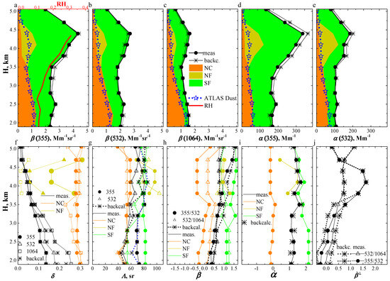
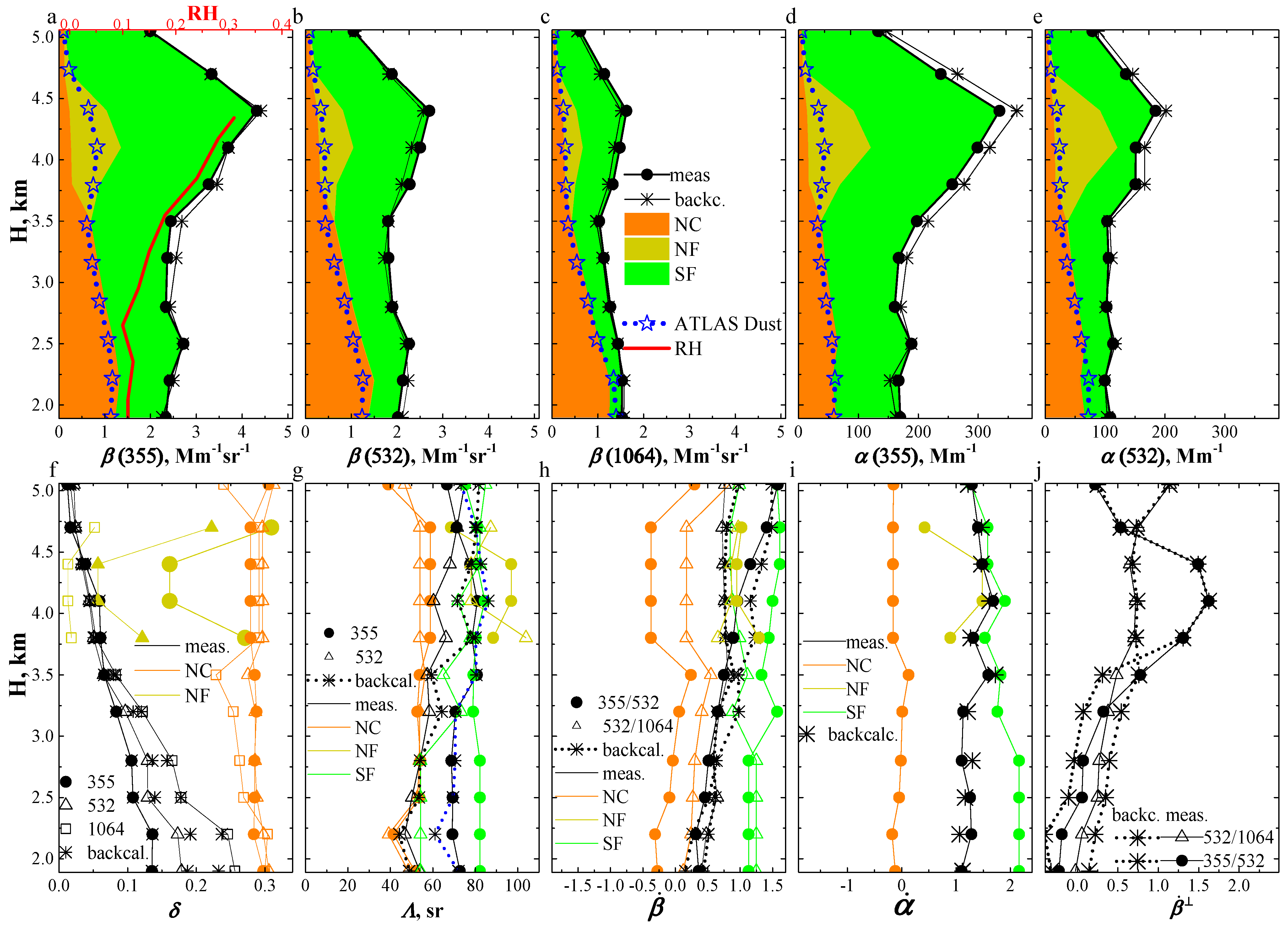
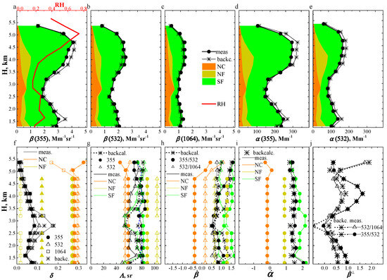
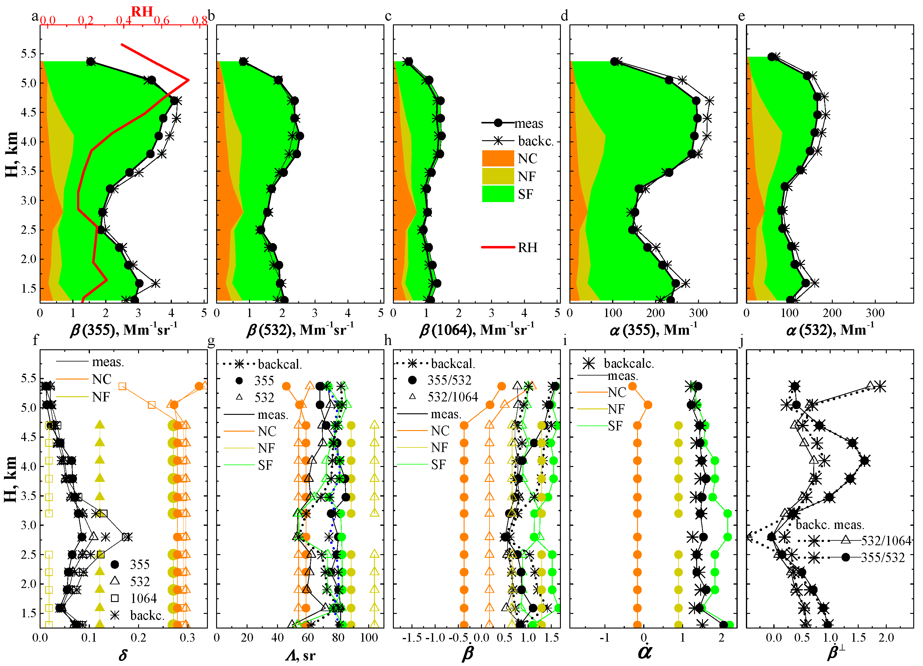
Figure 1 shows HSRL-2 measurements of the 3β + 2α + 3δ profiles (black curves with bullets, squares, and triangles) and the following profiles of the IPs:
Figure 1.
Measured (black curves with bullets, triangles, and squares) and backcalculated, i.e., retrieved total (asterisks), NF (olive), NC (orange), and SF (green) mode profiles of optical extensive (upper panel) and intensive parameters (lower panel) for measurement case I: (a) backscatter coefficient at 355 nm, (b) backscatter coefficient at 532 nm, (c) backscatter coefficient at 1064 nm, (d) extinction coefficient at 355 nm, (e) extinction coefficient at 532 nm, (f) PLDRs at 355, 532, and 1064 nm, (g) LRs at 355 and 532 nm, (h) BAE at the pair of wavelengths of 355 and 532 nm, and at the pair of wavelengths of 532 and 1064 nm, (i) EAE at the pair of wavelengths of 355 and 532 nm, (j) CrPBAE at the pair of wavelengths of 355 and 532 nm, and at the pair of wavelengths of 532 and 1064 nm. RH measurements are shown as a red curve. The blue curve corresponds to the dust profiles retrieved with ATLAS. See text for details.
- -
- extinction ()-related Ångström exponents (EAE) at the pair of wavelengths (355, 532) nm;
- -
- backscatter ()-related Ångström exponents (BAE) at the pairs of wavelengths (355, 532) and (532, 1064) nm;
- -
- lidar ratios (Λ) at 355 and 532 nm;
- -
- PLDRs (δ) at 355, 532, and 1064 nm;
- -
- cross-polarized backscatter ()-related Ångström exponents (CrPBAE) at the pairs of wavelengths (355, 532) and (532, 1064) nm.
The profiles consist of 11 height bins, which are equidistantly distributed between H = 1.9 and 5 km height above sea level with a vertical resolution of 310 m.
The profiles of the extensive optical data (see first row in Figure 1) are characterized by two maxima at 2.5 and 4.5 km, which can be attributed to a lower and an upper aerosol layer. The aerosol load of the upper layer peaks at 350 Mm−1 in terms of the extinction coefficient at 355 nm. The extinction coefficient does not exceed 200 Mm−1 in the lower layer.
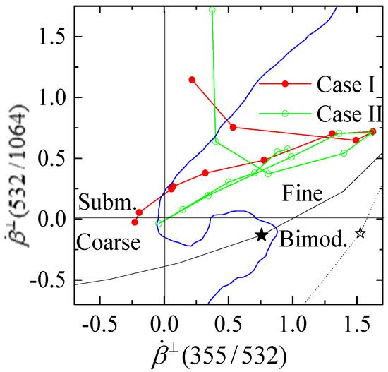
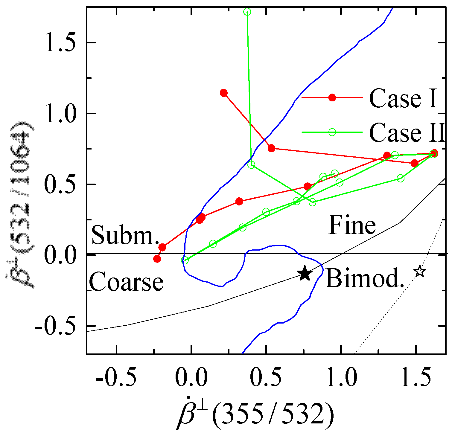
The profiles of the PLDRs decrease with height from δ(355) = 0.12, δ(532) = 0.18, and δ(1064) = 0.25 at 1.9 km to approximately 0 at all three wavelengths at 5 km (see black bullets, triangles, and squares in Figure 1f). At the same time, the spectrum of the PLDRs, i.e., their wavelength-dependent δ(λ), increases between 1.9 and 3.5 km height. As a result of this spectral behavior, sections of the profiles of the CrPBAEs are negative or slightly positive below 3.5 km (see triangles and bullets in Figure 1j). The profiles of δ(λ) are almost constant above 3.5 km height, and the values of (355/532) and (532/1064) simultaneously are positive in each height bin of the respective profiles. The interdependency of the CrPBAEs is cycloid-like if we include in our analysis the dependence of the profile (532/1064) versus the profile (355/532) (see red curves in Figure 2). From a theoretical point of view, these spectral and height-dependent signatures of the PLDRs and CrPBAEs indicate the presence of large non-spherical particles in the coarse mode of the PSDs below 3.5 km height above sea level. Furthermore, the results indicate that most of the non-spherical particles above 3.5 km height are in the fine/submicron mode of the investigated PSDs. Moreover, the hysteresis, i.e., the cycloid interdependency, indicates that the effective radius of one of the two modes changes.
Figure 2.
Interdependencies (532/1064) versus (355/532) for measurement case I (red) and measurement case II (green). The stars and black curves correspond to the synthetic CrPBAEs computed from the bimodal PSDs (see [1] for details).
The profile of the lidar ratio at 532 nm increases from 50 to 70 sr with height (see black curve with triangles in Figure 1g). In contrast, the profile of the lidar ratio at 355 nm varies between 70 and 80 sr below 4 km and decreases to 60 sr between 4 km and 5 km (see black curve with bullets in Figure 1g). The two profiles cross over at 4.7 km height, which indicates that particle sizes change with height.
The profile of the BAE at the wavelength pairs 355 and 532 nm (black curves with bullets) monotonically increases with height from 0.5 to 1.5. In contrast, the profiles of (black curves with bullets) and (532/1064) (black curves with triangles) slightly vary around 1.25 and 0.5, respectively, with height. The HSRL-2 3β + 2α + 3δ data are used as input in the ATLAS2.0 algorithm. Figure 1a–f shows the profiles measured with HSRL-2 (see black curves with bullets, triangles, and squares). The profiles are used for the retrieval of the particle optical and microphysical parameters.
3.1.1. Analysis of Measurement Case I with ATLAS2.0
Each height bin of the 3β + 2α + 3δ profiles has been analyzed by ATLAS2.0 separately. We start with the lowest height bin. Data in 11 height bins were processed in total.
Below 3.5 km, i.e., height bin numbers #1 to #6, the NM and NMSB strategies lead to discrepancies larger than 30%, and we reject the respective retrieval results. We furthermore reject solutions where these strategies result in two modes where the non-spherical particles (i.e., NBSB and NBSM PSDs) have zero imaginary part and a high real part (mR > 1.65) of the CRI.
In the case of the NSB strategy, we find acceptable solutions. The discrepancy (5) in this case fulfills condition (7) and varies between ρNSB = 6% and 7% below 3.5 km height. We obtain the following properties of the solution space at height bin #1, at 1.9 km height:
- The non-spherical part of the PSD (we denote the PSD in the following as NSB PSD) can be attributed to coarse mode particles, i.e., NM = NC. The fine-mode particles can be described by spheres, i.e., SM = SF. It means we obtain a bimodal PSD: NSB PSD = NM PSD + SM PSD.
- We find 275 elements (data records, datasets in the NRLUT) in the 5% vicinity of the NC mode solutions that fulfill the condition of minimal discrepancy ρNC,min = ρNM,min = 1% [see inequalities (7)]. Note: an extensive discussion on the topic of choosing the vicinity region (see previous sentences) can be found in Kolgotin et al. [24].
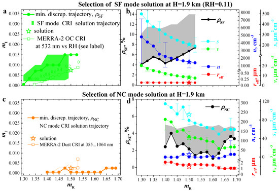
- The solution space of the NC mode is distributed between mR = 1.4 and 1.69 on the CRI-plane. The trajectory of the minimal discrepancy ρNC = ρNM(mR) increases from m = 1.4 − i0 to m = 1.69 − i0.0025 (solid orange curve with bullets). The rest of the solutions (orange-filled area) are spread along this trajectory, see Figure 3c. This spread, i.e., the uncertainty, extends from mI = i0.0025 to i0.01 at mR = 1.69. Simultaneously, the value of the global minimum is ρNC(mR) = 1% at m = 1.6 − 0. Four local minima of 2.1, 2.2, 1.5, and 2.5% can also be identified at m = 1.4 − i0, 1.45 − i0, 1.525 − i0, and 1.69 − i0.0025, respectively (see black curve in Figure 3d). Note: Figure 3a,b are projections of one and the same surface ρNC vs. (mR, mI), which can be presented as a 3-dimensional plot [24]. On this plot, the CRI solution trajectory is described by a “canyon”. However, in the present case, we use a two-dimensional projection for reasons of “simplicity”.Figure 3. Analysis of the solution space retrieved with ATLAS2.0 for SF mode (a,b) and NC mode (c,d) particles and the use of extra constraints for measurement case I at height level 1.9 km. The gray shaded areas describe discrepancies of individual solutions the CRI solution trajectories (see orange and green shaded areas) contain. The stars correspond to the final solution. See text for details.
- The solution space of the NC mode complies with the PPPOI. Effective radius (red solid line) decreases from reff = 2.1 µm at mR = 1.4 to 1.1 µm at mR = 1.69 along the trajectory of minimal discrepancy. Number concentration (blue solid line) increases at the same mR domain from n = 15 to 29 cm−3 along the trajectory defined by the two points at mR = 1.4 and mR = 1.69 (see Figure 3d). We note that the uncertainty of the complete solution space, which is defined by the 5% vicinity (see area in gray), results in a larger scatter of values from 1 to 4.3 µm for effective radius and from 2 to 100 cm−3 for number concentration.
- The 14% vicinity of the solution space of the SF mode contains 200 elements (records) in the SRLUT. This solution space corresponds to the minimal discrepancy ρSF,min = ρSM,min = 4% [see inequalities (7)].
- The solution space of the SF mode is distributed between mR = 1.3 and 1.525 on the CRI plane. The trajectory of the minimal discrepancy, i.e., ρSF = ρSM(mR), increases from m = 1.3 − i0 to m = 1.525 − i0.015 (solid green curve with bullets). The rest of the solutions (green area) are spread along the trajectory (see Figure 3a). The spread defines the uncertainty of the solution space, which extends from mI = i0.0075 to i0.02 at mR = 1.525. The global minimum of ρSF(mR) = 4% is located at m = 1.3 − i0. We find one local minimum of ρSF(mR) = 4.5% located at m = 1.4 − i0.01 (see black curve in Figure 3b).
- The effective radius of the SF mode (red solid curve) slightly decreases from reff = 0.121 µm at mR = 1.3 to 0.119 µm at mR = 1.525 along the trajectory of minimal discrepancy. The number concentration (blue solid curve) also decreases with mR in the same mR domain (see Figure 3b). However, this picture changes after we apply the CCN correction [26]. The trace nSF versus mR becomes a slightly increasing function, and simultaneously the spread of the solutions increases from 1100 to 2500 cm−3 at mR = 1.3 and from 1200 to 3000 cm−3 at mR = 1.525. This result means the solution space complies with the PPPOI for the SF-mode particles as well.
Our analysis of the solution spaces of the SF mode and the NC mode reveals a considerable uncertainty of the PMP retrievals for both modes of the bimodal PSD. To identify the final solution space, we again use the extra constraints on aerosol types (respectively, CRI) and relative humidity (see also Section 2). In view of the available a priori information, we attribute the NC and SF modes to dust and OC particles, respectively. The CRI of dust in MERRA-2 is m = 1.53 − i0.0026 at 532 nm, which is close to the value that belongs to the local minimum defined by ρNC(mR), i.e., m = 1.525 − i0 (see squares in Figure 3c). We select mNC = 1.5 − i0.0025 as the final solution. We note (1) the solution does not coincide with either the global or the local minima and (2) the discrepancy of the solution of ρNC(mR) = 3% exceeds the local minimum of 1.5% at m = 1.525 − i0. However, the imaginary part of the solution (mI = i0.0025) is the closest to the imaginary part of the CRI of dust in MERRA-2. Moreover, the part {3β + 2α}S, i.e., the contribution of spherical particles to the optical data, is physically meaningful at mNC = 1.5 − i0.0025 only.
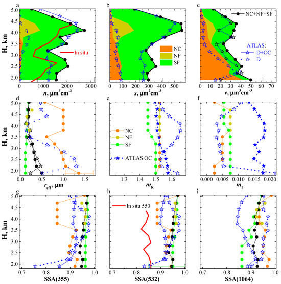
Unfortunately, knowledge about the aerosol type alone, i.e., the SF mode of the bimodal PSD that contains OC, is not sufficient because the retrieved solution space for OC contains all CRI values of the MERRA-2 model (see squares in Figure 3a). Therefore, we include another constraint, which is information about RH (see labels with the squares). RH is 0.11 at 1.9 km height, and the respective CRI of OC is m = 1.503 − i0.0077 at 532 nm in MERRA-2 (see red curve in Figure 1a). We select the point mSF = 1.5 − i0.0075 on the CRI solution trajectory. This point is close to m(532) = 1.503 − i0.0077 (see star in Figure 3a) and identifies the final solution with ρSF(1.5 − i0.0075) = 6.9%. The point mSF = 1.5 − i0.0075 is comparably far away from the minimal discrepancy trajectory that is defined by the point at m = 1.5 − i0.015 and ρSF(1.5 − i0.015) = 6.7% (see green bullets in Figure 3a and black bullets in Figure 3b), too. The rest of the PMPs, which correspond to mSF = 1.5 − i0.0075, are denoted with stars (see stars in Figure 3b). They almost coincide with respective solutions on the minimal-discrepancy trajectory (see bullets in Figure 3b). The uncertainty of the solution space of the retrieved SF mode and NC mode of the bimodal PSD is defined by the two points, mNC = 1.5 − i0.0025 and mSF = 1.5 − i0.0075, at 1.9 km (see error bars in Figure 3b,d and Figure 4d for effective radii). The uncertainty of the extensive PMPs (n, s, and v) of the bimodal PSD is the sum of the respective SF- and NC-mode uncertainties (see error bars in Figure 3b,d and Figure 4a–c).
Figure 4.
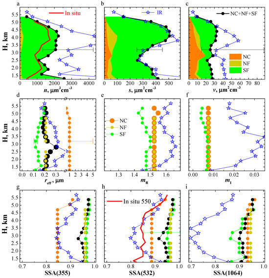
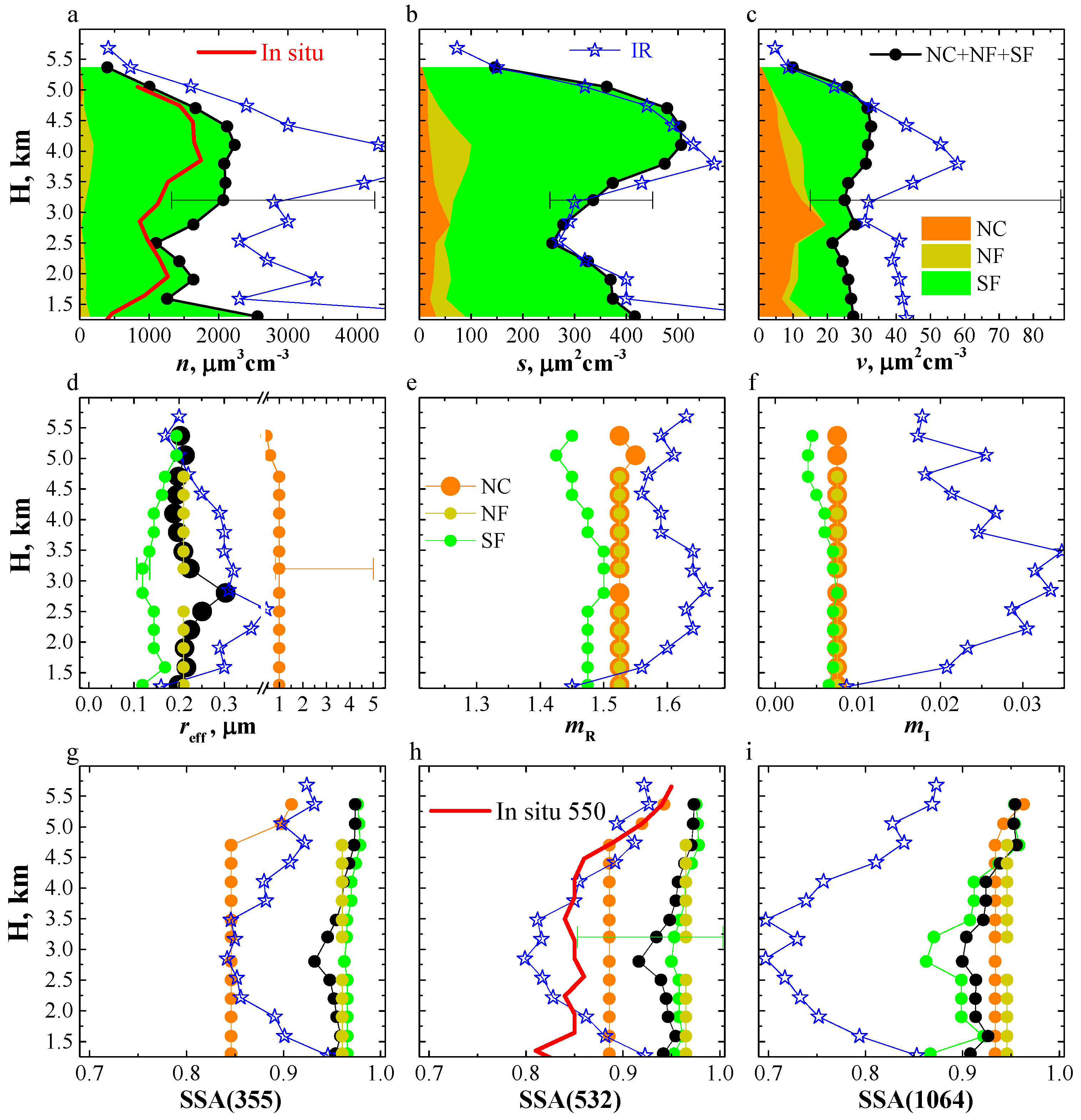
Profiles of the PMPs, CRIs, and SSA at 355, 532, and 1064 nm, retrieved with ATLAS2.0 (orange, olive, green, and black are for NC, NF, SF, and the total solutions) and ATLAS (stars) [22], and measured in situ (red) for measurement case I: (a) number concentration, (b) surface-area concentration, (c) volume concentration, (d) effective radius, (e) CRI real part, (f) CRI imaginary part, (g) SSA at 355 nm, (h) SSA at 532 nm, (i) SSA at 1064 nm. See text for details.
The NSB strategy delivers similar results at the height bins #2 to #6 and #11. The discrepancy ρNSB increases to more than 17% above 3.5 km height, except for the height bin at 5 km, i.e., the performance of the NSB strategy degrades, but it can be replaced with the solutions we find from the NBSM strategy. This strategy delivers solutions that are characterized by a lower range of discrepancies of ρNBSM,min = 7% to 9%. To localize the final set of solutions for each of the three modes, we analyze, as before, the trajectory of the CRI solution, and we apply the extra constraints. We assume that the particles in the NF mode are dust. Thus, the final solution space can be localized in the vicinity of the values mNF = mNC = 1.53 − i0.0026 to 1.53 − i0.007 for the wavelength range of [355; 1064] nm.
We note that the NBSB strategy also works in the upper part of the profile. However, the uncertainties of the solutions found with the NBSM strategy cover the results of both strategies. We also stress that 20 unknown parameters are determined from 8 pieces of measurement information (that is, 3β + 2α + 3δ datasets) in the case of the NBSB strategy., i.e., the mathematical problem is underdetermined, as it is characterized by a high degree of freedom and thus may have an infinite number of solutions (see the text on the crucial statement in [2] in Section 2.1). Therefore, the respective results are speculative.
3.1.2. Case I: Results and Discussion
The particle optical and microphysical profiles are retrieved with the ATLAS2.0 algorithm from the HSRL-2 3β + 2α + 3δ profiles (case I). The intensive optical profiles of the different modes are shown in Figure 1 in the second row, i.e., NC (orange), NF (olive; results are not always available, see previous section), and SF (green). Also shown in the first row of this figure are the extensive optical data, i.e., NC (orange area), NF (olive area), and SF (green area).
The backcalculated profiles of the optical data of the PLDR in the NC mode at 355, 532, and 1064 nm (see orange curves with bullets, triangles, and squares in Figure 1f, respectively) do not vary significantly. Values generally vary around 0.3 at all 3 wavelengths, with the exception that the profile of δ(1064) drops to approximately 0.25 at 3.5 and 5.0 km height. We explain the reason for this behavior in Section 3.1.2 (see retrieval of effective radius discussed in subpoint b). The PLDRs of the NF mode depend on wavelength (see olive curves with bullets, triangles, and squares in Figure 1f, respectively). The shorter the measurement wavelength, the higher the PLDR. In particular, the δ(λ) decreases from 0.16 to 0.01 with wavelength between 4.1 km and 4.4 km height. The PLDR profile of all components, i.e., the sum NC + NF + SF at 355 nm (asterisks), accurately reproduces the profile of δ(355) measured with HSRL-2. The PLDRs retrieved (also asterisks) and measured at 532 and 1064 agree within a few % uncertainty.
The profile of the CrPBAE retrieved at the pair of wavelengths 355 and 532 nm systematically underestimates the respective measured profile by 0.2 (see solid curve with asterisks in Figure 1j) below 3.5 km. In contrast, the profile of the CrPBAE retrieved at the wavelength pair 532 and 1064 nm systematically overestimates the respective measured profile by 0.2 in the same part of the profile (see dotted curve with asterisks in Figure 1j). However, the retrieved and measured profiles of (355/32) and (532/1064) nearly coincide above 3.5 km height. The reason for this result is the simultaneous use of the two equations for the estimation of the fractions of the NF mode and the NC mode at 355 and 532 nm [see Equation (1)].
The remaining IPs of the total profile (NC + NF + SF), i.e., the profiles of the LRs, BAEs, and EAE (see asterisks in Figure 1g–i), well reproduce the respective measured profiles. The retrieved modes can be described as follows:
- The LRs at 355 nm and 532 nm of the NC mode are similar and vary between 40 sr and 60 sr along the profiles (orange bullets and triangles, respectively, in Figure 1g). The difference between the profiles of the BAEs of the NC mode at the pairs of wavelengths (355; 532) nm and (532; 1064) nm is more obvious. The (355/532) profile (orange bullets) changes between −0.5 and 0, whereas the (532/1064) -profile (orange triangles in Figure 1h) is shifted toward larger values of 0 to 0.5. The EAE profile of the NC mode does not vary significantly. Values are approximately 0 (orange bullets in Figure 1i). These IPs (in the NC mode) are typical for large particles.
- The profiles of the LRs of the NF mode vary from 65 sr to 90 sr, and from 70 sr to 100 sr at 355 nm (olive bullets) and 532 nm (olive triangles in Figure 1g), respectively. The profiles of the (355/532) (olive bullets) and (532/1064) (olive triangles in Figure 1h) of the NF mode almost coincide. For example, we find a value of approximately 0.8 for both profiles at 4.1–4.7 km height. The difference between the BAE profiles is considerable at 3.8 km height. Values are 1.25 and 0.7 for the two profiles, respectively. The profile of the EAE of the NF mode varies from 0.4 to 1.5. These values of the IPs of the NF mode are typical for smaller, i.e., submicron particles.
- The profile of the LR of the SF mode at 355 nm (green bullets) decreases with height from 83 sr to 70 sr. In contrast, the profile of the LR at 532 nm (green triangles) increases with height from 55 sr to 85 sr (see Figure 1g). The profile of the BAEs of the SF mode varies insignificantly below 3 km height. Values are approximately 1.25. The profile of (355/532) (green bullets) increases to 1.6 above 3 km height. The profile of (532/1064) (green triangles) decreases to 0.75 in its upper part (see Figure 1h). The profile of the EAE of the SF mode decreases from 2.1 to 1.3 with height (see Figure 1i).
Figure 4, Figure 5 and Figure 6 show the retrieval results of the PMPs, CRIs, and SSA at 355, 532, and 1064 nm, split into the contributions by the NC, NF (if available), and SF mode, respectively. Also shown are the profiles of the sum of all three modes, i.e., the total profiles (NC + NF + SF). The extensive parameters of the NC (orange), NF (olive), and SF (green) modes are shown as colored (filled) areas (see Figure 4a–c and Figure 5).
Figure 5.
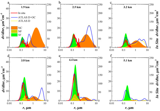
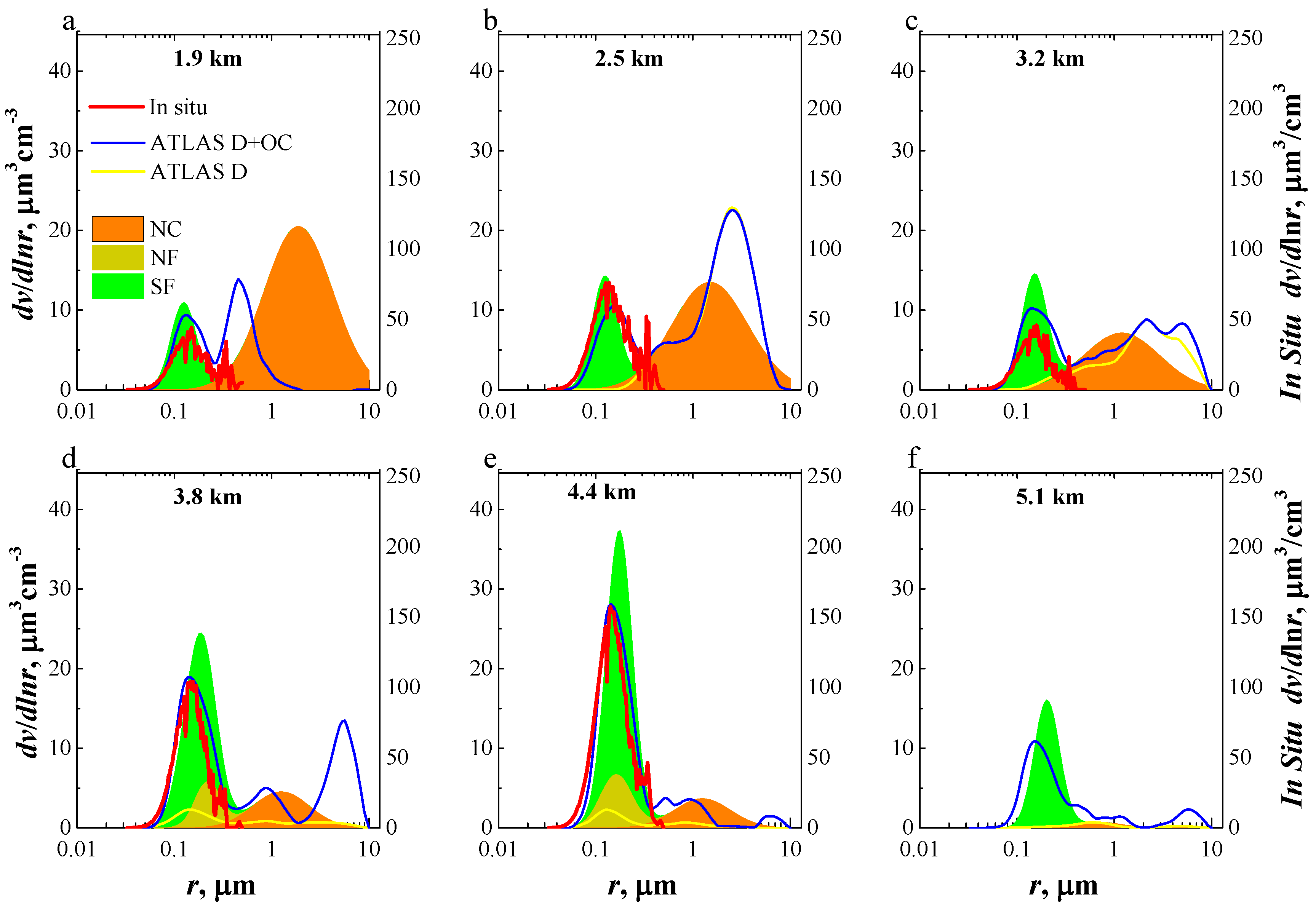
PSDs in [μm3 ⋅ cm−3] retrieved with ATLAS2.0 (orange, olive, and green areas) and ATLAS (blue and yellow curves) [22], and measured in situ (red) at (a) 1.9, (b) 2.5, (c) 3.2, (d) 3.8, (e) 4.4, (f) 5.1 km for measurement case I. See text for details.
Figure 6.
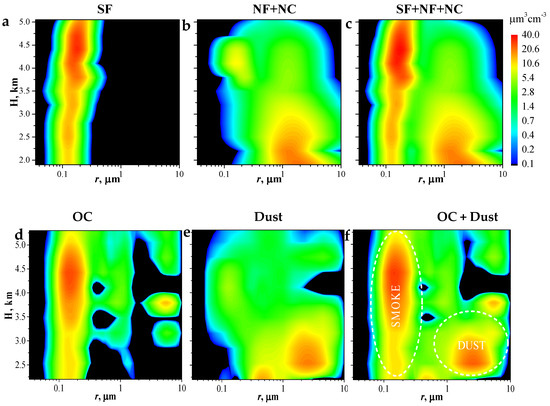
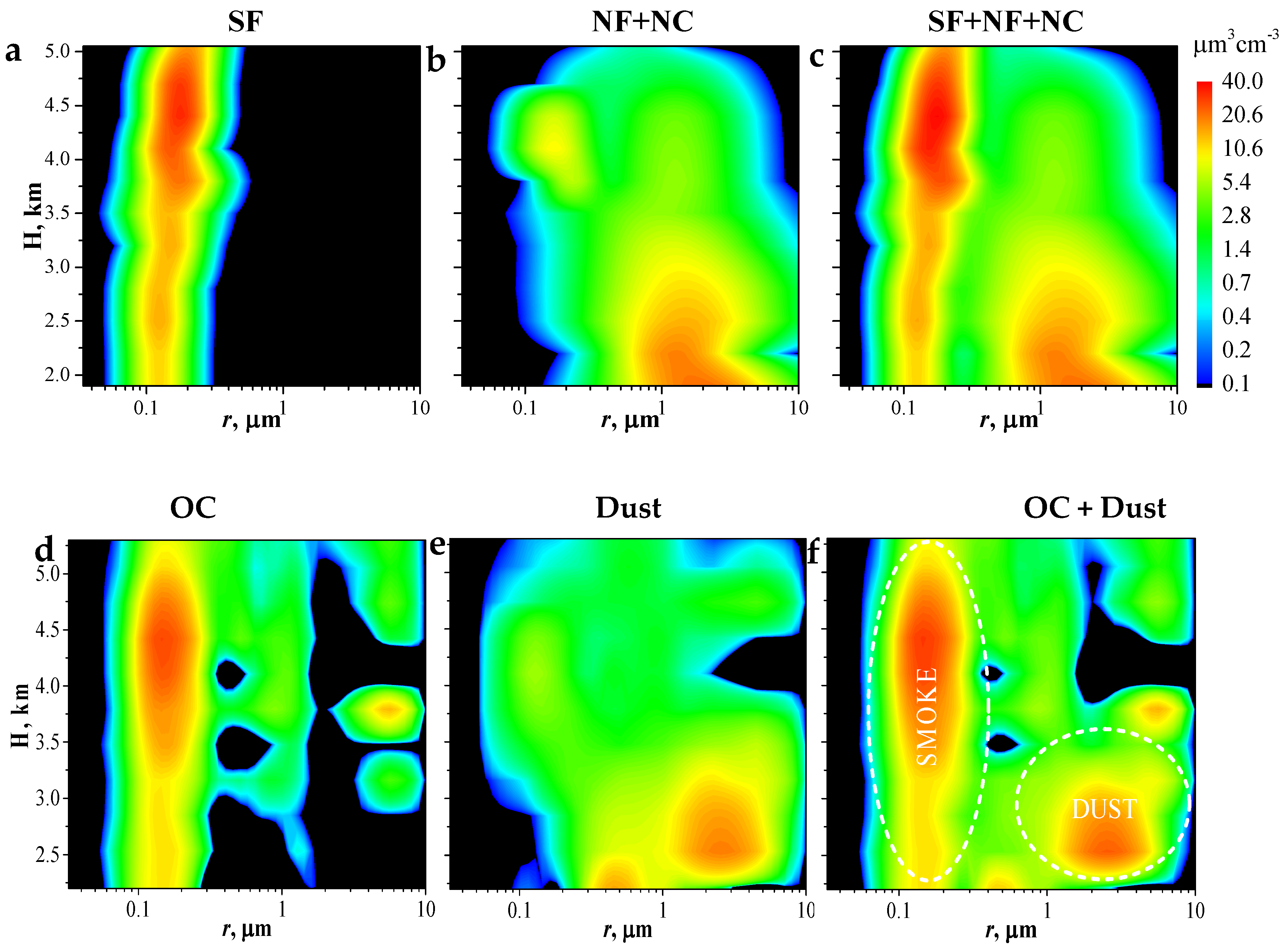
PSDs in [μm3 ⋅ cm−3] versus height retrieved with ATLAS2.0 (a–c) and ATLAS (d–f) [22] for measurement case I.
Figure 4d–i show the profiles of the intensive parameters of the SF mode (green curves with bullets), NC mode (orange curves with bullets), NF mode (olive curves with bullets), and the sum of all modes (apart from the CRIs), i.e., the total profile (black curves with bullets). The retrieval results are as follows:
- The total profiles of the extensive PMPs (see bullets in Figure 4a–c) are characterized by two maxima at 2.5 and 4.5 km height if we exclude the lowest height bin, where measurement errors are larger than on average. These profiles reproduce comparably well the profiles of the extensive optical data that were acquired with HSRL-2. The maximal values of number and surface-area concentration are 2800 cm−3 and 550 µm2cm−3, respectively, in the upper aerosol layer. In contrast, the maximal volume concentration of 40 µm3cm−3 is attained in the lower particle layer. Total effective radius decreases with height from 0.5 to 0.25 µm. The total SSA slightly depends on wavelength and height. The average value of the SSA in this profile is close to 0.95 at 532 nm.
- Profiles of the surface-area and volume concentrations of the NC mode particles (see orange in Figure 4a–c) decrease with height. The maximum values are 91 µm2cm−3 and 41 µm3cm−3 at 1.9 km height. The concentrations drop to negligible values at 5 km height. The number concentration of the NC mode is comparably low. The maximum value is 151 cm−3 at 3.5 km height. The average value of the effective radius in the profile of the NC mode is close to 1 µm (see orange curve in Figure 4d).
The effective radius of the NC mode considerably deviates from this average value in the 3 height bins at 1.9, 3.5, and 5.1 km. The deviations at 1.9 and 3.5 km most likely are caused by comparably large measurement errors. The lowest height bin of the profile is 1.9 km above ground, and it is the most distant one from the airborne lidar. The outlier at 3.5 km coincides with an outlier of the data in the EAE profile at the same height level (see black curve in Figure 1i). More details about the quality of the optical data taken with HSRL-2 in the ORACLES campaign are given by Kolgotin et al. [27].
The comparably low value of the effective radius of 0.5 µm at 5.1 km, which in fact represents the minimum value of effective radius throughout the profile, can be explained theoretically. The interdependency between the CrPBAEs in the upper part of the profile is cycloid-like, which means, from a theoretical point of view [1], that the size of the non-spherical particles changes (see red curves in Figure 2). The CRI of the NC mode corresponds to the values of dust in MERRA-2, i.e., m = 1.51…1.53 − i0.002…0.007, which were used as extra constraints. The SSA profiles of the NC mode follow the shape of the mI profile, i.e., the larger the imaginary part, the lower is the SSA and vice versa. We note that even small changes in the mI, i.e., less than 0.005, may lead to considerable variations in the SSA, i.e., from 0.85 to 0.95 at 355 nm.
- c.
- In contrast to the results for the NC mode, number, surface-area, and volume concentrations of the SF mode (see green curve in Figure 4a–c) are increasing or slightly variable with height up to 5 km. The maximum values are 1900 cm−3, 410 µm2cm−3, and 23 µm3cm−3, respectively, in the height range of 4.1–4.4 km. The effective radius of the SF mode increases with height from 0.12 to 0.19 µm (see green curve in Figure 4d). This result can be linked to the increase in RH with height from 0.1 to 0.3 (see red curve in Figure 1a). Simultaneously, the CRI of the SF mode decreases from 1.5 − i0.0075 in the lower aerosol layer to 1.45 − i0.0055 in the upper aerosol layer, which also could be the result of increasing humidity, i.e., water uptake by hygroscopic particles in the fine mode fraction of the PSDs. The SSA of the SF mode slightly increases with height from 0.95 to 0.97 at 355 and 532 nm, respectively. The variations in SSA at 1064 nm are larger. Its profile increases with height from 0.86 to 0.94.
- d.
- The particles of the NF mode contribute only to the aerosol load in the upper aerosol layer (see olive curves). The intensive parameters of the NF mode are close to or coincide with the intensive parameters of the SF mode (see Figure 4d–i). In contrast, the values of the extensive parameters are between the values of the extensive parameters of the NC and SF modes (see Figure 4a–c), respectively.
- e.
- The total PSD is bimodal in the lower part of the profile and trimodal in the upper part of the profile (see Figure 5 and Figure 6c). The coarse mode of the PSD is solely represented by non-spherical particles and dominates the lower aerosol layer. We find a peak value of 20 µm3cm−3 of the volume concentration for a modal radius of 2 µm. The volume concentration of the coarse mode drops in the upper aerosol layer. The maximum value is 0.7 µm3cm−3 for a modal radius of 0.7 µm (see orange in Figure 5). The fine mode of the bimodal PSD (see green curve in Figure 5) contains spherical particles in the lower aerosol layer. The fine mode of the trimodal PSD contains a mixture of non-spherical (see area filled by olive in Figure 5) and spherical particles in the upper aerosol layer. The peak values of the volume concentration and modal radius increase with height from 10 to 37 µm3cm−3 and from 0.12 to 0.17 µm, respectively. These maxima are reached at 4.4 km height.
3.2. Case Study II: Measurement from 20 September 2016, 11:47–12:24 UTC
We use the same approach as described in Section 3.1 for the analysis of the measurement case II. Figure 7 shows the optical data retrieved with ATLAS2.0 and taken by lidar. Figure 8 shows the retrieved profiles of the PMPs, CRIs, and SSA at 355, 532, and 1064 nm. Figure 9 and Figure 10 show the results of the PSD retrievals. We find similar structures in the profiles of the optical data taken with lidar and obtained from ATLAS2.0 for both case I and case II. Therefore, we will only discuss points where the results differ between case II and case I.
Figure 7.
Same as Figure 1, but for measurement case II: (a) backscatter coefficient at 355 nm, (b) backscatter coefficient at 532 nm, (c) backscatter coefficient at 1064 nm, (d) extinction coefficient at 355 nm, (e) extinction coefficient at 532 nm, (f) PLDRs at 355, 532 and 1064 nm, (g) LRs at 355 and 532 nm, (h) BAE at the pair of wavelengths of 355 and 532 nm, and at the pair of wavelengths of 532 and 1064 nm, (i) EAE at the pair of wavelengths of 355 and 532 nm, (j) CrPBAE at the pair of wavelengths of 355 and 532 nm, and at the pair of wavelengths of 532 and 1064 nm.
Figure 8.
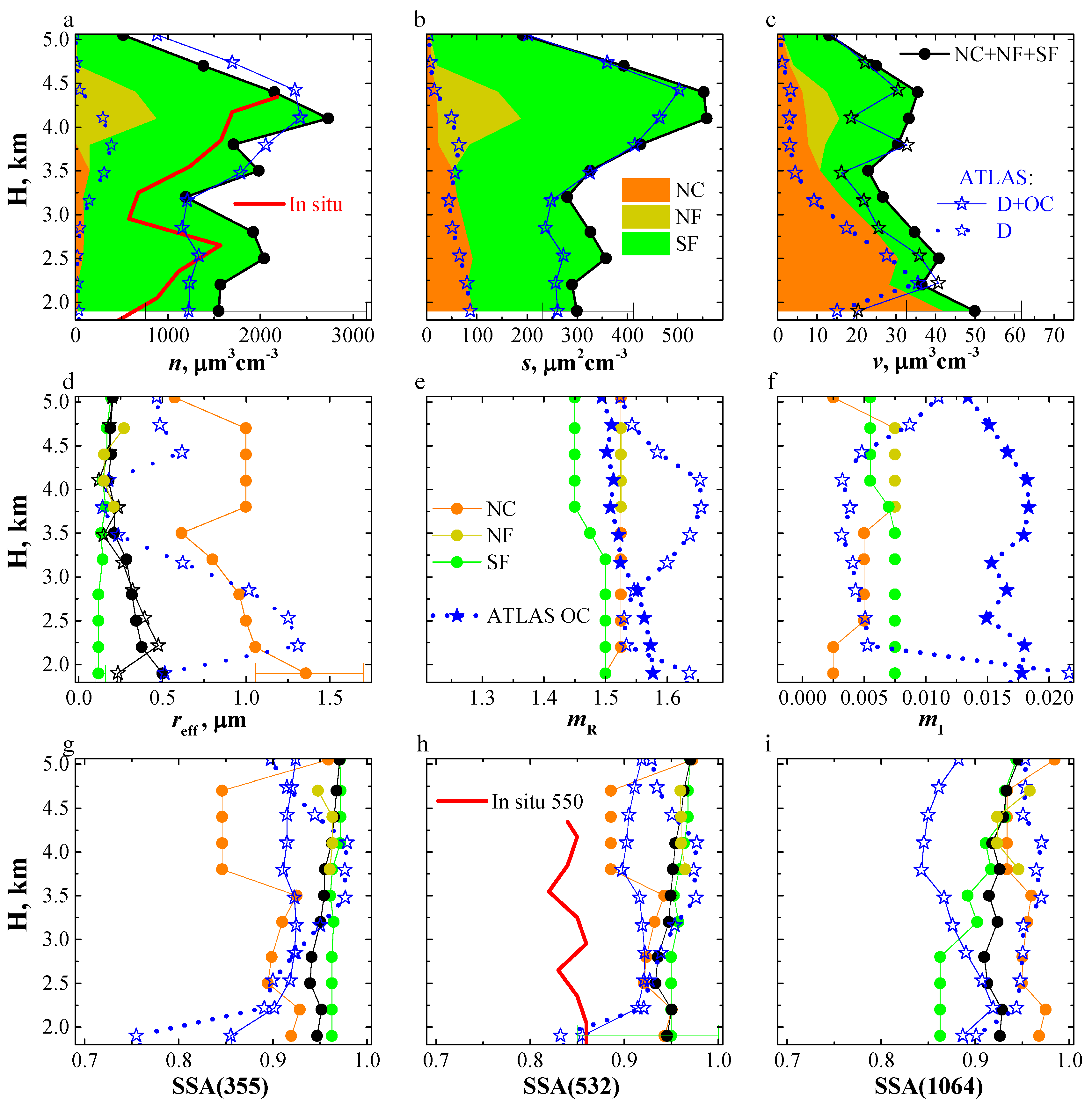
Same as Figure 4 but for measurement case II: (a) number concentration, (b) surface-area concentration, (c) volume concentration, (d) effective radius, (e) CRI real part, (f) CRI imaginary part, (g) SSA at 355 nm, (h) SSA at 532 nm, (i) SSA at 1064 nm. In this case, IR (blue) is used for the comparison of the retrieval results instead of the ATLAS results. The CRI retrieved with IR is given in terms of the total PSD.
Figure 9.
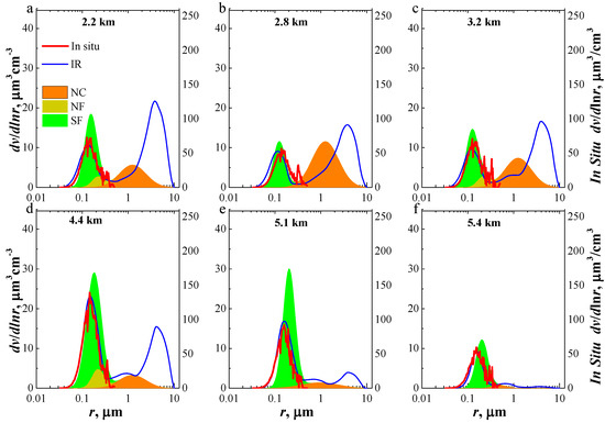
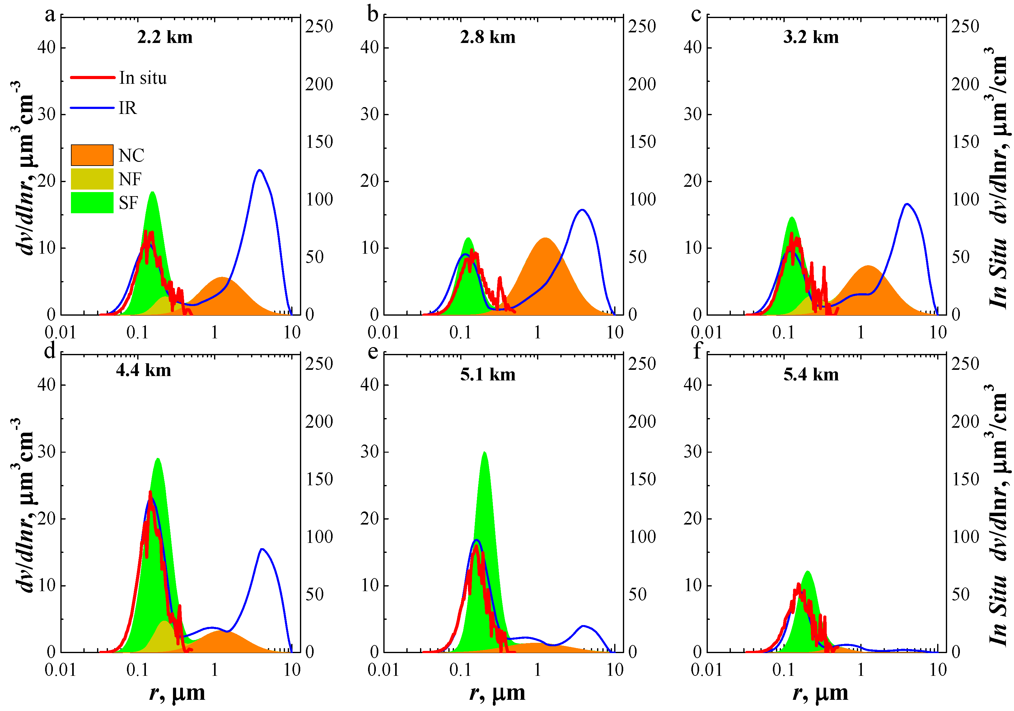
PSDs in [μm3 cm−3] retrieved with ATLAS2.0 (area filled by orange, olive, and green) and the results obtained from inversion with regularization (blue curves) [20], and measured in situ (red) at (a) 2.2, (b) 2.8, (c) 3.2, (d) 4.4, (e) 5.1, (f) 5.4 km for measurement case II. See text for details.
Figure 10.
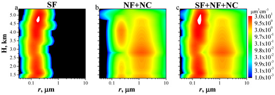
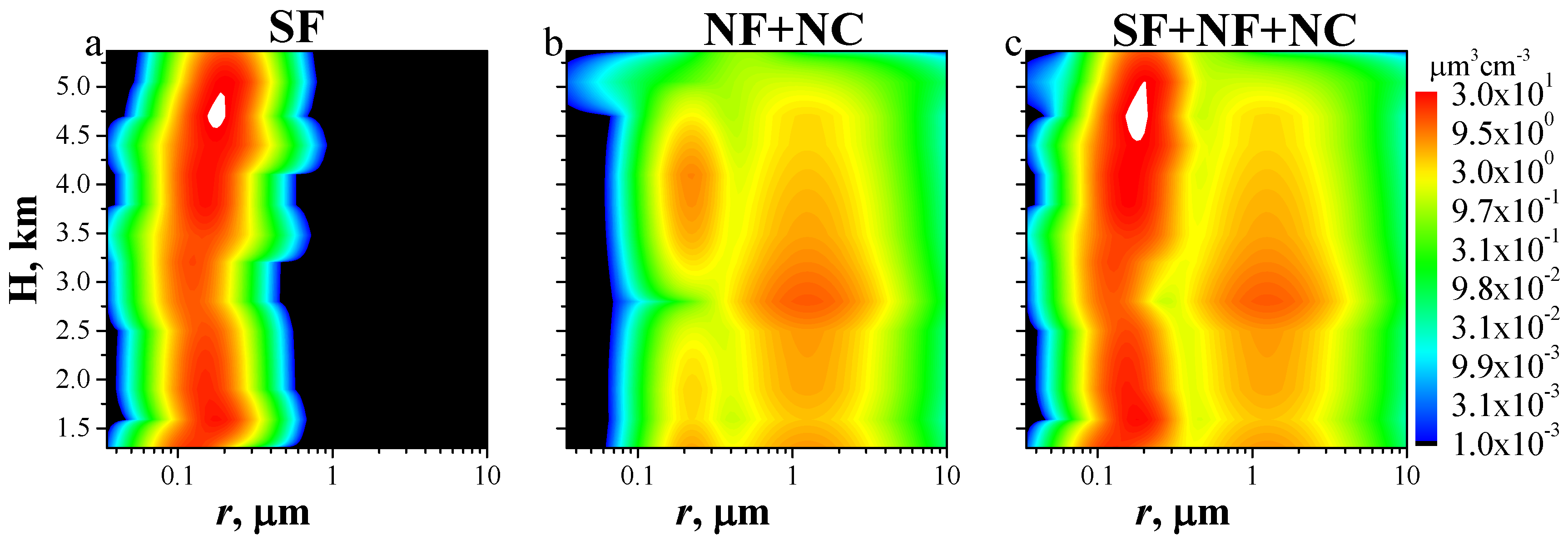
PSDs in [μm3 cm−3] versus height retrieved with ATLAS2.0 for measurement case II. Shown are the results for the (a) SF and (b) NF + NC modes and (c) for the mixture.
The PLDR profiles of the two cases show a comparably minor difference. The maximum values are δ(355) = 0.09, δ(532) = 0.11, and δ(1064) = 0.17 in case II. These values, which are lower than 0.12, 0.18, and 0.25 in case I, respectively, are reached at 2.8 km. The PLDRs monotonically decrease from that height level upward and downward and reach 0.05 at 5.5 km height and 0.05 at 1.6 km height. However, in both cases (I and II), the interdependencies of the CrPBAEs are similar and characterized by a hysteresis in the upper part of the profiles (see Figure 2). The hysteresis, though very narrow in width, can also be seen below 5.5 km height.
Another minor difference is the use of different ATLAS2.0 strategies for the retrieval of the PMPs. The NSB strategy works only at 2.8, 5.1, and 5.4 km for case II, i.e., at heights where the PLDRs reach their maximal and minimal values. The NBSM strategy works for all other height bins. As a result, the profile of the tri- and bimodal PSDs is dominated by coarse-mode non-spherical particles, i.e., the contribution by coarse-mode particles is maximal at 2.8 km height, and it drops below and above 2.8 km.
4. Discussion
We discuss the results obtained in our study and put them into context with the results obtained from previous investigations. We compare the PMPs, CRIs, and SSAs retrieved with the ATLAS2.0 algorithm for both measurement cases to the respective results retrieved with alternative inversion techniques, which have been published before, i.e., IR [21] and ATLAS [4], and the in situ observations. A detailed description of the results retrieved with ATLAS for case I can be found in Kolgotin et al. [22]. Results retrieved with IR for case II are presented by Kolgotin et al. [20]. Results of in situ observations of both cases are presented in detail by Kolgotin et al. [20]. Figure 1, Figure 4, Figure 5 and Figure 8, and 9 show the results retrieved with ATLAS (blue curves and yellow solid curves) and IR (blue curve), respectively. Data taken in situ are represented by red curves in these figures. ATLAS permits us to estimate the parameters of each aerosol type separately, i.e., OC and dust particles (blue dotted curves), as the two cases describe external particle mixtures. The results of the total parameters of the complete mixture, i.e., OC + D, are shown, too (blue solid curves). We will start with the discussion of case I.
As shown in Figure 1, the optical properties of D and OC derived with ATLAS are consistent with those obtained with ATLAS2.0 for both NC- and SF-mode particles at altitudes below 3.5 km. Above 3.5 km, the results obtained with ATLAS and ATLAS2.0 also agree well if we attribute some part of the NF mode particles to D particles and the rest of the particles of the NF mode to OC particles. The CRI of m = 1.53 − i0.0026 of dust in MERRA-2 has been used as a constraint for the PMP retrieval of the NF-mode particles. The value of the CRI is quite close to the CRI of m = 1.47 − i0.006 of OC in MERRA-2. Thus, in view of the retrieval uncertainty for the NF mode, these D fine-mode particles can be attributed to OC particles, too. The PLDRs of the NF- and SF-mode mixture are approximately δ(355) = 0.04, δ(532) = 0.02, and δ(532) = 0.003 and agree comparably well with values for smoke particles [28].
The profiles of number, surface-area, and volume concentration of OC + D retrieved with ATLAS slightly underestimate the respective profiles retrieved with ATLAS2.0 (see Figure 4a–c). The effective radii of the complete PSDs (OC + D) retrieved with both approaches agree comparably well in all height bins of the profile except for the height bin at 1.9 km, where the measurement errors are larger than on average (see Figure 4d). The differences in the retrieval results between the PMPs of the D (OC) in the case of ATLAS and NC (SF) modes in the case of ATLAS2.0 are larger, but we still find similarities in terms of the qualitative behavior, i.e., the shape of the respective profiles. We find a comparably large difference for the results of the CRI obtained with ATLAS and ATLAS2.0 (see Figure 4e,f). The real part of the CRI of dust and the imaginary part of the CRI of organic carbon retrieved with ATLAS are larger than the real part (of the NC-mode particles) and imaginary part (of the SF-mode particles) retrieved with ATLAS2.0. The differences are 0.15 and i0.015 for the real and imaginary parts, respectively. This result shows that these 3β + 2α + 3δ datasets do not allow us to make robust estimations of the CRI without the use of extra constraints. The large difference between the two CRI-retrieval results leads to considerable differences between the total SSA obtained with ATLAS and ATLAS2.0. The maximal differences reach 0.05, 0.06, and 0.1 at 355, 532, and 1064 nm, respectively.
The fine modes of the PSDs retrieved with ATLAS and ATLAS2.0 are characterized by similar peak values of the extensive parameters and modal radii (see Figure 5 and Figure 6). The differences do not exceed 20%. The differences between the coarse modes retrieved by both approaches are larger than the ones for the fine modes, but remain within the uncertainties. Moreover, the PSDs retrieved with ATLAS may contain another, fourth mode. As we mentioned before, the competitive NBSB strategy of ATLAS2.0 delivers a similar fourth mode and thus four modal PSDs in the upper part of the profiles, too.
The profiles of the PMPs and CRIs retrieved with IR for case II systematically overestimate the respective profiles retrieved with ATLAS2.0 (see Figure 8a–f). As a result, the SSA profiles retrieved with IR are systematically lower than the respective profiles retrieved with ATLAS2.0 (see Figure 8g–i). The peak values and modal radii of the fine mode of the PSDs retrieved with IR are also lower than the respective parameters retrieved with ATLAS2.0. The differences are 10–40% and 5–10%, respectively (see Figure 9). In contrast, the coarse modes of the PSDs retrieved by IR are considerably larger than the coarse modes obtained with ATLAS2.0. In fact, the method of IR uses Lorenz–Mie light-scattering theory, i.e., spherical-particle geometry. In the case of non-spherical particles, IR leads to an overestimation of the volume concentration and CRI of the coarse-mode particles [10].
The number concentrations measured in situ are lower than the values we obtain for this parameter with ATLAS2.0 for both measurement cases. On average, the differences in number concentrations stay below 25% throughout the profile (see Figure 4a and Figure 8a). We find a similar average overestimation of the peak values of the fine mode of the volume PSDs (see Figure 5). The modal radii of the fine mode of the PSDs are quite similar for both techniques. The SSA retrieved with the ATLAS2.0 algorithm at 532 nm is systematically larger compared to the SSA measured in situ at 550 nm. The differences are as large as 0.1 for cases I and II (see Figure 4h and Figure 8h).
We also investigated whether these differences in SSA can be reduced. In fact, the PPPOI permits us to consider arbitrary CRIs on the solution trajectory. One of the SF-mode solutions of case I is m = 1.525 − i0.02 at 1.9 km height (see Figure 3a). This CRI leads to an SSA of approximately 0.85 at 532 nm (see error bar in Figure 4h), which is similar to the in situ values. However, the number concentration simultaneously increases (see error bars), and values come closer to the solution retrieved with IR [20]. That means the number concentration is significantly larger than the number concentration obtained from the in situ observations. In other words, the PMPs and the CRI, which simultaneously agree with the in situ data, are located on different parts of the solution trajectory. We derived the same result in one of our recent studies [29]. This result, i.e., the PMPs and CRI are on different parts of the solution trajectory, is caused by the fact that we use an incorrect particle shape and thus a flawed light-scattering model for the retrieval algorithm. In view of this result, we therefore hypothesize that we can simultaneously retrieve correct CRIs and PMPs from lidar measurements if and only if the correct particle shape is known. Finally, another reason for the differences between the SSAs measured in situ and retrieved by ATLAS2.0 can be the assumption of a spectrally independent CRI in ATLAS2.0. We will include the option to apply a wavelength-dependent CRI in a future version of ATLAS2.0.
The comparison we carried out in this section shows that number concentrations and PSDs derived by the different techniques (ATLAS2.0, ATLAS, IR, and in situ) converge. These results allow us to verify the performance capability of ATLAS2.0 and validate the respective retrieval products. The retrieval accuracy of SSA (CRI) obtained by ATLAS2.0 can be further improved if we include accurate information about particle shape and the wavelength dependence of the CRI [30].
5. Conclusions
We present examples of the use of the ATLAS2.0 algorithm for the analysis of data collected by multiwavelength high-spectral-resolution lidar 2 (HSRL-2). ATLAS2.0 has been specially developed for the application of a model of randomly oriented spheroids in the context of the retrieval of non-spherical particle microphysical parameters from 3β + 2α + 3δ lidar measurements. The theoretical background of ATLAS2.0 has been presented by Kolgotin and Müller [1,2]. We selected 2 case studies of 3β + 2α + 3δ data collected by HSRL-2 and used ATLAS2.0 to retrieve profiles of PMPs and SSA from HSRL-2 measurements. The data were taken on 20 September 2016 between 10:14 and 10:29 UTC (case I) and 20 September 2016 between 11:47 and 12:24 UTC (case II) in the framework of the ORACLES campaign in southwestern Africa [ORACLES database: https://espoarchive.nasa.gov/archive/browse/oracles/id8/ER2 (accessed on 1 February 2025)]. These two cases are characterized by moderate-to-high PLDRs of δ(355) = 0.09–0.14, δ(532) = 0.11–0.19, and δ(1064) = 0.19–0.26. Our analysis of the CrPBAEs shows hysteresis, i.e., a cycloid-like interdependency of (532/1064) versus (355/532).
Data analysis shows the presence of particles in the NC, NF, and SF modes in both measurement cases. Both cases are characterized by two aerosol layers, respectively. In both cases, the volume concentration of the NC-mode particles reaches its maximum in the lower aerosol layer (below 3 km height) and decreases in the upper aerosol layer (above 3 km height). In contrast, the volume concentration of the NF-mode particles increases with height. However, both (NC and NF) modes disappear in the upper height bins. The results show that only non-spherical particles in the submicron size range are present above 4.5–5 km. This result explains why the effective radius of the fraction of the non-spherical particles varies with height.
The contribution of particles in the SF mode increases with height up to 4.5 km in both cases. We see increasing values of number, surface-area, and volume concentrations. The effective radius of particles of the SF mode varies along the profile in a similar fashion to that of RH, which was measured during the ORACLES campaign, too.
ATLAS2.0 furthermore provides us with results on the NBSM PSDs. These PSDs describe the sum of all particles in the various types of modes, i.e., NC + NF + SF. ATLAS2.0 allows us to estimate the respective PMPs and SSAs. The results confirm that particle PLDRs at 355, 532, and 1064 nm measured with lidar contain significant information about particle size and the PSDs themselves.
We furthermore compare our results to results obtained from other retrieval methods, namely, ATLAS, inversion with regularization, and information obtained from in situ observations of the aerosol layers. This comparison allows us to test, verify, and, in part, validate the results obtained with ATLAS2.0. All solutions converge within the retrieval uncertainties. The profiles of number concentrations and PSDs, retrieved with ATLAS2.0 and measured in situ, agree within an average 25% uncertainty. Simultaneously, the discrepancy between the measured and backcalculated, i.e., retrieved 3β + 2α + 3δ data on average does not exceed 10%, and the maximum difference is 17%. We find a significant difference of, on average, 0.1 between SSA retrieved with ATLAS2.0 and measured in situ. We hypothesize that a correct SSA (and as a result, the CRIs) and PMPs can be simultaneously retrieved from lidar measurements if and only if the correct particle shape is known.
The PLDRs at 355, 532, and 1064 nm measured with lidar and reproduced with ATLAS2.0 agree, but convergence of the optical datasets (experimental versus backcalculated) can only be achieved if the aerosol particles are considered as a sphere–spheroid mixture. Similarity of the PLDR spectrum measured with lidar and reproduced with ATLAS2.0 allows balancing the results derived (a) theoretically with a model of randomly oriented spheroids and (b) experimentally with state-of-the-art measurement techniques.
For further validation of the results, we will investigate in future studies if
- -
- ATLAS2.0 is applicable to PMP retrievals of more/other aerosol types from different regions in the world;
- -
- whether the retrieval results can be improved by using a wavelength-dependent CRI and more complicated geometries of particle shape.
Author Contributions
Methodology, A.K.; formal analysis and investigation, A.K. and D.M.; writing—original draft preparation, A.K.; writing—review and editing, D.M. and A.K.; supervision and resources, D.M. All authors have read and agreed to the published version of the manuscript.
Funding
This research received no external funding.
Data Availability Statement
Data is unavailable due to privacy restrictions.
Acknowledgments
We thank the NASA Langley HSRL-2 team for providing the data used in our study. All data can be downloaded from publicly accessible databases. The website is http://espoarchive.nasa.gov/archive/browse/oracles (accessed on 1 February 2025).
Conflicts of Interest
The authors declare no conflicts of interest.
Abbreviations and Denotations
The following abbreviations and denotations are used in this manuscript:
| α | particle extinction coefficient |
| β | particle backscatter coefficient |
| β⊥ | particle cross-polarized backscatter coefficient |
| g | particle backscatter or extinction coefficient |
| δ | particle linear depolarization ratio (PLDR) |
| δ′ | particle depolarization potential |
| ζ | particle scatter coefficient |
| λ | wavelength |
| extinction-related Ångström exponent (EAE) | |
| backscatter-related Ångström exponent (BAE) | |
| cross-polarized BAE (CrPBAE) | |
| ε | relative deviation |
| e | relative measurement error |
| Δ | absolute deviation |
| A | ratio of two extinction coefficients |
| H | height above sea level |
| B | ratio of two backscatter coefficients |
| Λ | lidar ratio (LR) |
| LN | lognormal function |
| m | complex refractive index |
| mR | CRI real part |
| mI | CRI imaginary part |
| dv(r)/dlnr | volume particle size distribution (PSD) |
| n | number concentration |
| s | surface-area concentration |
| volume concentration | |
| r | radius |
| r0 | mean radius |
| reff | effective radius |
| σ | standard deviation (Gauss parameter) |
| μ | mean radius (Gauss parameter) |
| fraction | |
| ρ | discrepancy |
| P | Parameter |
| C | coarse |
| CRI | complex refractive index |
| CCN | cloud condensation nuclei |
| D | dust |
| IR | inversion with regularization |
| F | fine |
| IP | intensive parameter |
| N | non-spherical shape |
| M | monomodal |
| NSB | non-spherical–spherical bimodal |
| NMSB | non-spherical monomodal–spherical bimodal |
| NBSM | non-spherical bimodal–spherical monomodal |
| NBSB | non-spherical bimodal–spherical bimodal |
| NRLUT | reference look-up table for the spheroids |
| OC | organic carbon |
| ODQA | optical data quality assurance |
| PMP | particle microphysical parameters |
| PPPOI | principle of polydisperse particle optical invariance |
| RLUT | reference look-up table |
| RH | relative humidity |
| S | spherical shape |
| SRLUT | reference look-up table for the spheres |
| SS | spheres and spheroids |
| SSA | single-scattering albedo |
References
- Kolgotin, A.; Müller, D. Model of randomly oriented spheroids for the retrieval of non-spherical particle microphysical parameters from 3β+2α+3δ lidar measurements, part 1: Structure and analysis of information content of central spheroid look-up table. Remote Sens. 2026, 18, 1595. [Google Scholar] [CrossRef] [Scilit]
- Kolgotin, A.; Müller, D. Model of randomly oriented spheroids for the retrieval of non-spherical particle microphysical parameters from 3β+2α+3δ lidar measurements, part 2: ATLAS (version 2.0) retrieval algorithm. Remote Sens. 2026; submitted.
- Kolgotin, A.; Müller, D.; Chemyakin, E.; Romanov, A. Improved identification of the solution space of aerosol microphysical properties derived from the inversion of profiles of lidar optical data, part 2: Simulations with synthetic optical data. Appl. Opt. 2016, 55, 9850–9865. [Google Scholar] [CrossRef] [Scilit]
- Kolgotin, A.; Müller, D. Aerosol Typing from Linear estimations for the Analytical Separation (ATLAS) of complex aerosol mixtures and improved identification of microphysical parameters from multiwavelength lidar data, part 1: Theory and numerical simulation. J. Opt. Soc. Am. A 2025, 42, 221–232. [Google Scholar] [CrossRef] [Scilit]
- Ansmann, A.; Müller, D. Lidar and atmospheric aerosol particles. In Lidar: Range-Resolved Optical Remote Sensing of the Atmosphere; Weitkamp, C., Ed.; Springer: New York, NY, USA, 2005; pp. 105–142. [Google Scholar]
- Hair, J.W.; Hostetler, C.A.; Cook, A.L.; Harper, D.B.; Ferrare, R.A.; Mack, T.L.; Welch, W.; Izquierdo, L.R.; Hovis, F.E. Airborne High Spectral Resolution Lidar for profiling aerosol optical properties. Appl. Opt. 2008, 47, 6734–6752. [Google Scholar] [CrossRef] [Scilit]
- Mishchenko, M.I.; Travis, L.D. T-matrix computations of light scattering by large spheroidal particles. Opt. Commun. 1994, 109, 16–21. [Google Scholar] [CrossRef] [Scilit]
- Yang, P.; Liou, K.N. Geometric-optics-integral-equation method for light scattering by nonspherical ice crystals. Appl. Opt. 1996, 35, 6568–6584. [Google Scholar]
- Dubovik, O.; Sinyuk, A.; Lapyonok, T.; Holben, B.N.; Mishchenko, M.; Yang, P.; Eck, T.F.; Volten, H.; Muñoz, O.; Veihelmann, B.; et al. Application of spheroid models to account for aerosol particle nonsphericity in remote sensing of desert dust. J. Geophys. Res. 2006, 111, D11208. [Google Scholar] [CrossRef] [Scilit]
- Veselovskii, I.; Dubovik, O.; Kolgotin, A.; Lapyonok, T.; Di Girolamo, P.; Summa, D.; Whiteman, D.N.; Mishchenko, M.; Tanré, D. Application of randomly oriented spheroids for retrieval of dust particle parameters from multiwavelength lidar measurements. J. Geophys. Res. 2010, 115, D21203. [Google Scholar] [CrossRef] [Scilit]
- Soupiona, O.; Samaras, S.; Ortiz-Amezcua, P.; Böckmann, C.; Papayannis, A.; Moreira, G.A.; Benavent-Oltra, J.A.; Guerrero-Rascado, J.L.; Bedoya-Velásquez, A.E.; Olmo, F.J.; et al. Retrieval of optical and microphysical properties of transported Saharan dust over Athens and Granada based on multi-wavelength Raman lidar measurements: Study of the mixing processes. Atmos. Environ. 2019, 214, 116824. [Google Scholar] [CrossRef] [Scilit]
- Saito, M.; Yang, P.; Ding, J.; Liu, X. A Comprehensive database of the optical properties of irregular aerosol particles for radiative transfer simulations. J. Atmos. Sci. 2021, 78, 2089–2111. [Google Scholar] [CrossRef] [Scilit]
- Saito, M.; Yang, P. Advanced bulk optical models linking the backscattering and microphysical properties of mineral dust aerosol. Geophys. Res. Lett. 2021, 48, 2021GL095121. [Google Scholar] [CrossRef] [Scilit]
- Chang, Y.; Hu, Q.; Goloub, P.; Podvin, T.; Veselovskii, I.; Ducos, F.; Dubois, G.; Saito, M.; Lopatin, A.; Dubovik, O.; et al. Retrieval of microphysical properties of dust aerosols from extinction, backscattering and depolarization lidar measurements using various particle scattering models. Atmos. Chem. Phys. 2025, 25, 6787–6821. [Google Scholar] [CrossRef] [Scilit]
- Holben, B.N.; Eck, T.F.; Slutsker, I.; Smirnov, A.; Sinyuk, A.; Schafer, J.; Giles, D.; Dubovik, O. AERONET’s Version 2.0 quality assurance criteria. Proc. SPIE 2006, 6408, 134–147. [Google Scholar] [CrossRef] [Scilit]
- Müller, D.; Veselovskii, I.; Kolgotin, A.; Tesche, M.; Ansmann, A.; Dubovik, O. Vertical profiles of pure dust and mixed smoke-dust plumes inferred from inversion of multiwavelength Raman/polarization lidar data and comparison to AERONET retrievals and in situ observations. Appl. Opt. 2013, 52, 3178–3202. [Google Scholar] [CrossRef] [Scilit]
- Das, S.; Colarco, P.R.; Bian, H.; Gassó, S. Improved simulations of biomass burning aerosol optical properties and lifetimes in the NASA GEOS model during the ORACLES-I campaign. Atmos. Chem. Phys. 2024, 24, 4421–4449. [Google Scholar] [CrossRef] [Scilit]
- Harshvardhan, H.; Ferrare, R.; Burton, S.; Hair, J.; Hostetler, C.; Harper, D.; Cook, A.; Fenn, M.; Scarino, A.J.; Chemyakin, E.; et al. Vertical structure of biomass burning aerosol transported over the southeast Atlantic Ocean. Atmos. Meas. Tech. 2022, 22, 9859–9876. [Google Scholar] [CrossRef] [Scilit]
- Pistone, K.; Redemann, J.; Doherty, S.; Zuidema, P.; Burton, S.; Cairns, B.; Cochrane, S.; Ferrare, R.; Flynn, C.; Freitag, S.; et al. Intercomparison of biomass burning aerosol optical properties from in-situ and remote-sensing instruments in ORACLES-2016. Atmos. Chem. Phys. 2019, 19, 9181–9208. [Google Scholar]
- Kolgotin, A.; Müller, D.; Korenskiy, M.; Veselovskii, I. ORACLES campaign, September 2016: Inversion of HSRL-2 observations with regularization algorithm into particle microphysical parameters and comparison to airborne in situ data. Atmosphere 2023, 14, 1661. [Google Scholar] [CrossRef] [Scilit]
- Veselovskii, I.; Kolgotin, A.; Griaznov, V.; Müller, D.; Franke, K.; Whiteman, D.N. Inversion of multiwavelength Raman lidar data for retrieval of bimodal aerosol size distribution. Appl. Opt. 2004, 43, 1180–1195. [Google Scholar] [CrossRef] [Scilit] [PubMed]
- Kolgotin, A.; Müller, D.; Goloub, P.; Hu, Q.; Podvin, T.; Wang, X. Aerosol Typing from Linear estimations for the Analytical Separation (ATLAS) of complex aerosol mixtures and improved identification of microphysical parameters from multiwavelength lidar data, part 2: Case studies. J. Opt. Soc. Am. A 2025, 42, 233–253. [Google Scholar] [CrossRef] [Scilit] [PubMed]
- Wang, A.; Yin, Z.; Mao, S.; Wang, L.; Yi, Y.; Chen, Q.; Müller, D.; Wang, X. Measurements of particle extinction coefficients at 1064 nm with lidar: Temperature dependence of rotational Raman channels. Opt. Exp. 2024, 32, 4650–4667. [Google Scholar] [CrossRef] [PubMed]
- Kolgotin, A.; Müller, D.; Romanov, A. Particle microphysical parameters and the complex refractive index from 3β + 2α HSRL/Raman lidar measurements: Conditions of accurate retrieval, retrieval uncertainties and constraints to suppress the uncertainties. Atmosphere 2023, 14, 1159. [Google Scholar] [CrossRef] [Scilit]
- Veselovskii, I.; Goloub, P.; Podvin, T.; Tanré, D.; da Silva, A.; Colarco, P.; Castellanos, P.; Korenskiy, M.; Hu, Q.; Whiteman, D.N.; et al. Characterization of smoke/dust episode over West Africa: Comparison of MERRA-2 modeling with multiwavelength Mie-Raman lidar observations. Atmos. Meas. Tech. 2018, 11, 949–969. [Google Scholar] [CrossRef] [Scilit] [PubMed]
- Mamouri, R.-E.; Ansmann, A. Potential of polarization lidar to provide profiles of CCN- and INP-relevant aerosol parameters. Atmos. Chem. Phys. 2016, 16, 5905–5931. [Google Scholar]
- Kolgotin, A.; Müller, D.; Veselovskii, I.; Korenskiy, M.; Wang, X. Pre-filter analysis for retrieval of microphysical particle parameters: A quality-assurance method applied to 3 backscatter (β) +2 extinction (α) optical data taken with HSRL/Raman lidar. Appl. Opt. 2023, 62, 5203–5223. [Google Scholar] [CrossRef] [Scilit]
- Burton, S.P.; Hair, J.W.; Kahnert, M.; Ferrare, R.A.; Hostetler, C.A.; Cook, A.L.; Harper, D.B.; Berkoff, T.A.; Seaman, S.T.; Collins, J.E.; et al. Observations of the spectral dependence of linear particle depolarization ratio of aerosols using NASA Langley airborne High Spectral Resolution Lidar. Atmos. Chem. Phys. 2015, 15, 13453–13473. [Google Scholar] [CrossRef] [Scilit]
- Kolgotin, A.; Müller, D.; Mona, L.; D’Amico, G. TiARA (Version 2.1): Simulations of particle microphysical parameters retrievals based on MERRA-2 synthetic organic carbon–dust mixtures in the context of multiwavelength lidar data. Remote Sens. 2026, 18, 658. [Google Scholar] [CrossRef] [Scilit]
- Di Biagio, C.; Formenti, P.; Balkanski, Y.; Caponi, L.; Cazaunau, M.; Pangui, E.; Journet, E.; Nowak, S.; Andreae, M.O.; Kandler, K.; et al. Complex refractive indices and single scattering albedo of global dust aerosols in the shortwave spectrum and relationship to size and iron content. Atmos. Chem. Phys. 2019, 19, 15503–15531. [Google Scholar] [CrossRef] [Scilit]
Disclaimer/Publisher’s Note: The statements, opinions and data contained in all publications are solely those of the individual author(s) and contributor(s) and not of MDPI and/or the editor(s). MDPI and/or the editor(s) disclaim responsibility for any injury to people or property resulting from any ideas, methods, instructions or products referred to in the content. |
© 2026 by the authors. Licensee MDPI, Basel, Switzerland. This article is an open access article distributed under the terms and conditions of the Creative Commons Attribution (CC BY) license.