


Highlights
What are the main findings?
- Maximum tillering (∼79 DAS) ranked among the top three UAV windows for CH4, N2O and CO2, with GLCM textures carrying the gain; PlanetScope instead peaked at Midand Late-boot (103–107 DAS), where vegetation indices alone explained the flux.
- Nested Leave-One-Plot-Out validation reached between +0.57 and +0.69 for four of the six platform × gas combinations, and the UAV thermal mean (Tmean) was decisive for N2O ().
What is the implication of the main findings?
- Phenological windows can be matched to what each sensor actually resolves (texture-rich tillering for the UAV, boot-stage canopy for PlanetScope), so remote GHG monitoring of AWD rice on the Peruvian north coast does not need to be spread evenly across the season.
- UAV–CH4 and PlanetScope–N2O remained weak, so the workflow needs multi-site and multi-season testing before it is used to report fluxes operationally under AWD irrigation.
Abstract
Alternate wetting and drying (AWD) irrigation reduces CH4 emissions from flooded rice but amplifies N2O pulses; identifying candidate phenological windows for the remote screening of greenhouse gas (GHG) fluxes remains challenging with small datasets. In a single-site, single-season exploratory study at INIA Vista Florida (Lambayeque, Peru), eight UAV flights were paired with eight PlanetScope SuperDove scenes ( d) and closed-chamber CH4, N2O and CO2 fluxes under four water regimes (CF, AWD5, AWD10, AWD20; 96 sub-plot × date observations). Multivariate explanatory power was assessed by bootstrap Ridge regression on each sensor’s native predictors (VI + GLCM + for the UAV, VI for PlanetScope). Maximum tillering (79 DAS) emerged as a candidate UAV window, ranking in the top three for all gases through GLCM textures, whereas PlanetScope peaked at Mid-boot and Late-boot (103–107 DAS), with median at – and at –. Nested Leave-One-Plot-Out (LOPO) validation gave between and for four of six platform × gas combinations (UAV-CH4 and Planet-N2O stayed weak), and was decisive for N2O on the UAV (). Repeating the stage selection inside every LOPO fold preserved the leading combinations and their ranking. These exploratory windows and sensor-native descriptors need multi-site, multi-season validation before operational use.
1. Introduction
Flood-irrigated rice (Oryza sativa L.) accounts for approximately 10 % of global anthropogenic methane (CH4) emissions and is also a significant source of nitrous oxide (N2O) when managed under partial-aeration regimes [1,2]. As a mitigation response, alternate wetting and drying (AWD) irrigation has been promoted internationally to reduce CH4 emissions from flooded rice by introducing short soil-drying cycles [3,4]. However, the N2O pulses associated with soil rewetting and the heterogeneous yield response across treatments make the spatial and temporal quantification of greenhouse gas (GHG) fluxes under AWD a persistent scientific and operational challenge, particularly in South American rice systems where empirical evidence remains scarce [5,6,7].
Closed-chamber GHG flux monitoring, although accurate, is constrained by its low spatial density and high logistical cost, which prevents it from capturing the within- and between-plot variability typical of rice systems under AWD. Remote sensing from unmanned aerial vehicles (UAVs) and from high-cadence satellite constellations such as PlanetScope addresses this limitation by providing repeated observations of biophysical variables that covary with biogeochemical processes: leaf area index, chlorophyll content, canopy cover and structural heterogeneity [8,9,10]. Multispectral UAV platforms enable centimetre-scale canopy characterisation [11,12], whereas the PlanetScope SuperDove constellation (8 bands, 3 m GSD) extends observation to the catchment scale at a daily revisit, opening the possibility of remote-sensing-assisted monitoring at regional scale subject to multi-site validation [9,10].
Vegetation indices (VIs) are common predictors of rice biophysical variables: NDVI [13], the chlorophyll-sensitive GNDVI [14], the soil-background-corrected OSAVI [15] and EVI2, which mitigates saturation in dense canopies [16], are widely used in UAV-based rice monitoring [12,17,18,19]. More recently, textural features derived from the gray-level co-occurrence matrix (GLCM) [20] have emerged as complementary descriptors: they capture canopy structural heterogeneity that purely spectral indices fail to resolve [21,22,23]. Combining spectral and textural descriptors mitigates VI saturation at advanced phenological stages and improves the estimation of biophysical variables that are indirectly related to GHG fluxes, such as biomass and canopy nitrogen status [11,21,24,25,26,27].
This link is, however, indirect: spectral and textural indices describe canopy structure and pigment status, whereas CH4 and N2O fluxes are governed by soil-process variables (soil moisture, redox potential, microbial activity and labile carbon and nitrogen availability) that the canopy reflects only partially. Optical descriptors therefore act as proxies that co-vary with, rather than cause, the underlying biogeochemistry, and a satellite signal correlated with paddy growth need not imply a causal link with the emitted gas [28]; this distinction is maintained throughout.
The predictive ability of VIs and GLCM textures is not uniform across the cropping cycle: it varies between phenological stages in response to changes in canopy structure, nitrogen status and the plant water balance [29,30,31]. Identifying a priorithe phenological window with the highest explanatory power, rather than fitting models over the entire cycle, has been shown to improve the parsimony of the final models and to reduce the overfitting risk in small datasets [31,32,33]. In rice, the tillering stage concentrates the maximum between-plot differentiation in biomass, cover and nitrogen status [4,7], while the reproductive stage governs canopy closure and the residual nitrogen response [17,33]. Despite this agronomic knowledge, the explicit link between phenological stage, multivariate predictive ability of VI + GLCM and chamber-measured GHG fluxes under AWD has rarely been quantified in the literature.
Reliable estimation of the multivariate explanatory power of remote-sensing descriptors in small agronomic datasets requires statistical approaches that can control spectral multicollinearity and reduce overfitting. Ridge regression has been widely used as a stable estimator under small sample sizes and correlated predictors because it penalises the ℓ2 norm of the coefficients and reduces the variance of the fit [18,19,25]. When combined with bootstrap resampling, this approach enables the uncertainty of the multivariate to be quantified across phenological stages and allows predictor sets to be compared under the same sample size and regularisation framework, thereby supporting the relative ranking of stages [31,32]. Related studies in rice systems have shown that UAV- and satellite-derived vegetation indices can explain leaf nitrogen, biomass and yield with values of approximately 0.6–0.8 in paddy environments across India, China and Southeast Asia [27,34,35,36]. At broader spatial scales, satellite-observed methane has also been linked to paddy growth dynamics, although such associations remain correlative rather than causal [28]. For final predictive modelling, algorithms such as Random Forest, XGBoost [37], Support Vector Regression and Partial Least-Squares Regression [38,39,40] have been increasingly adopted, but their evaluation requires spatially blocked validation schemes, such as Leave-One-Plot-Out (LOPO), to prevent information leakage between training and test folds in clustered field experiments [41,42,43,44]. Despite these advances, direct chamber-referenced relationships between remote-sensing descriptors and the three major greenhouse gas fluxes under alternate wetting and drying remain scarcely documented, particularly in South American rice systems.
Building on this gap, the overall objective of this study was to assess when, and with which sensor-native remote-sensing descriptors, chamber-measured GHG fluxes are most explainable in an AWD rice system on the Peruvian coast. The specific objectives were to: (i) identify, using bootstrap Ridge regression, the phenological stages with the highest multivariate for each gas, platform and predictor set; (ii) develop predictive models for these selected stages using multiple machine-learning algorithms under nested Leave-One-Plot-Out (LOPO) cross-validation; and (iii) quantify the contribution of vegetation indices and texture descriptors to identify the dominant predictors for each gas. The main contribution of this study is a chamber-referenced ranking of phenological windows and sensor-native descriptors for CH4, N2O and CO2 fluxes under AWD. The UAV and PlanetScope pairing, the textural and thermal descriptors and the cross-validation design are the components that enable this framework rather than separate claims of novelty, providing a methodological and empirical basis for advancing phenology-informed, field-validated remote monitoring of GHG dynamics in rice systems.
2. Materials and Methods
2.1. Study Site and Experimental Design
The experiment was carried out at the INIA Vista Florida experimental station (6.7517°S; 79.8272°W; 50 m a.s.l.; Lambayeque, north coast of Peru; Figure 1) during the February–June 2023 rice campaign (transplanting on 3 February 2023; harvest between 2 June 2023 and 7 June 2023). Four water-management treatments were evaluated: continuous flooding (CF) and three AWD regimes whose re-flooding thresholds were triggered when the water table dropped to 5, 10 or 20 cm below the soil surface (AWD5, AWD10 and AWD20, respectively). The experiment was laid out in four main plots (one per treatment) of 24 × 11 m (264 m2), each split into three sub-plots of 8 × 11 m (88 m2) that constitute the independent experimental unit of the study (12 sub-plots in total: 3 sub-plots × 4 treatments). Fertilisation inputs were uniform across treatments. Irrigation events were gauged on an event-by-event basis through measurements of flow velocity, hydraulic section and water depth in each main plot, and were added to rainfall inputs recorded as water-table changes in each sub-plot.
Figure 1.
Study site: (a) continental location; (b) regional location in Lambayeque (Peru); (c) experimental plots and GHG chambers at INIA Vista Florida.
Table 1 consolidates the seasonal totals per treatment. Cumulative water savings relative to CF were 13.7 %, 14.9 % and 20.1 % for AWD5, AWD10 and AWD20, within the ranges reported for AWD in rice [1,2]; fertilisation supplied 320.7 kg N ha−1 (urea, five applications between DAS 38 and DAS 110), 167.5 kg P ha−1 (Terraphos, four applications) and 30.0 kg K ha−1 (KCl, single application at DAS 38), identical across the four treatments.
Table 1.
Water-management treatments and seasonal totals of water and fertilisation applied during the 2023 rice campaign at INIA Vista Florida.
2.2. Greenhouse Gas Flux Measurements
CH4, N2O and CO2 fluxes were measured with the non-vented closed static chamber method [6,45,46], deployed on a perimeter base previously installed in each of the 12 sub-plots (3 replicates × 4 treatments) on 8 sampling dates aligned with the UAV flights. The chamber is built from opaque polyethylene to inhibit photosynthesis during the incubation and consists of two coupled sections (Figure 2): a perforated base with regularly spaced openings that allow water exchange with the surrounding floodwater, and an upper drum that is hermetically coupled to the base through a hydraulic seal that ensures a watertight closure during sampling. The drum is fitted with (i) a side gas-sampling port consisting of a silicone hose connected to a three-way stopcock and a 60-mL polypropylene syringe for the manual extraction of headspace aliquots, (ii) a top thermometer that records the internal chamber temperature [47], and (iii) a small fan powered by a portable USB battery that ensures homogeneous mixing of the gas phase during the incubation [6,46].
Figure 2.
Opaque non-vented closed static chamber used for the measurement of CH4, N2O and CO2 fluxes: (a) front view with dimensions and components; (b) operation modes (monitoring and sampling); (c) base detail with hydraulic seal. Adapted from [6].
Sampling was carried out on the same day as each nitrogen fertilisation event, three days afterwards, and at 15-day intervals thereafter, capturing changes associated with crop phenology and water management. The event-anchored design (sampling at each fertilisation and three days later) was intended to bracket the early part of the post-fertilisation pulses, while the 15-day routine cadence kept the manual gas-chromatography workload feasible over the full cycle in twelve sub-plots. We nonetheless acknowledge that a 15-day routine interval can underestimate the short, episodic N2O peaks that follow fertilisation and rewetting, which evolve on hourly-to-daily timescales [48,49]; the implications of this temporal undersampling for the weaker N2O models are discussed in Section 4. All campaigns were conducted in the morning (08:00–11:00 local time) under clear-sky conditions. For each sampling date, four headspace aliquots were withdrawn at , 20, 40 and 60 min after chamber closure [6] and transferred immediately to 15-mL pre-evacuated borosilicate glass vials sealed with a rubber septum (Exetainer, Labco Limited, Lampeter, UK); the vials were kept in the dark and processed within 14 days. The concentration of the three gases in each aliquot was quantified by gas chromatography on a GC-2014 instrument (Shimadzu Corporation, Kyoto, Japan), equipped with a flame ionisation detector (FID) for CH4 and CO2 (with methanation when applicable) and an electron-capture detector (ECD) for N2O, at the Greenhouse Gas Laboratory of the Alliance of Bioversity International and CIAT (Cali, Colombia) [6,47]. The detectors were calibrated against a multi-point series of certified standards spanning the concentration ranges expected in flooded and AWD-managed rice; quality-control checks included ambient-air blanks and an intermediate-concentration standard injected per analytical batch. Gas fluxes were computed by linear regression of concentration against time following the standard formulation , with corrections for chamber air temperature and atmospheric pressure at the time of sampling, and expressed as mg CH4-C m−2 h−1, mg N2O-N m−2 h−1 and mg CO2 m−2 h−1 [46]; whenever the linear regression showed systematic curvature of concentration against time, the non-linear adjustment based on the Hutchinson and Mosier method [45] was applied, following the practice recommended by the Global Research Alliance to avoid flux underestimation under headspace saturation [46].
The total number of sub-plot–date observations used for modelling was 96 (8 dates × 12 sub-plots; per treatment). The eight phenological stages recorded (Active tillering, Mid-tillering, Late tillering, Maximum tillering, Mid-boot, Late-boot, Mid-heading, End of heading; equivalent to BBCH 21–69 [50]) were grouped into two agronomic phases for the stratified analyses, following the partitions consolidated in recent UAV multispectral and hyperspectral rice monitoring studies [29,30]: the vegetative phase (DAS 42–79: the four tillering stages), considered a key window because of its spectral sensitivity and its role in the dynamics of methane and nitrous oxide pulses under AWD management [4,7], and the reproductive phase (DAS 103–127: booting and anthesis), where canopy cover stabilises and red-edge indices capture the nitrogen response of the crop under intermittent flooding and waterlogging [33]; each phase comprises four flights.
2.3. UAV Acquisitions and Processing
A DJI Matrice 300 RTK UAV (SZ DJI Technology Co., Ltd., Shenzhen, China) equipped with an RTK module for centimetre-level positioning was operated with two complementary payloads in a dual gimbal configuration: (i) a Parrot Sequoia multispectral camera (Parrot SA, Paris, France) with four narrow bands (Green 530–570 nm, Red 640–680 nm, Red Edge 730–740 nm, NIR 770–810 nm) and an upward-facing incident-irradiance sensor (sunshine sensor) mounted on top of the UAV; and (ii) a Zenmuse H20T payload (DJI, Shenzhen, China), a multi-sensor unit that integrates a wide-angle RGB camera (12 MP, FOV 82.9°), a hybrid 23× zoom RGB camera (20 MP, equivalent focal length 31.7–877.7 mm) and a radiometric VOx microbolometer thermal sensor (640 × 512 pixels, 13.5 mm focal length, FOV 40.6°, NETD ≤ 50 mK at f/1.0, accuracy ±2 °C, thermal range −40 to +150 °C in high-gain mode), which delivers factory-calibrated brightness temperature in R-JPEG format. Sequoia reflectance was calibrated using the incident-irradiance sensor and a static calibration panel measured before and after each flight; the radiometric response of the H20T is internal to the payload and does not require an external thermal panel.
Eight flights were carried out between 15 February and 11 May 2023 (Table 2), with the following acquisition parameters: flight altitude 45 m above ground, speed 1.5 m s−1, forward overlap of 85% and side overlap of 80%. The 45 m altitude was chosen as a compromise that keeps the multispectral ground sampling distance fine enough to resolve within-plot canopy structure (∼4.7 cm/pixel for the Sequoia and ∼1.5 cm/pixel for the resampled H20T thermal ortho-mosaic) while covering the whole experimental block in a single safe flight line under the local airspace constraints; lower altitudes would have multiplied the number of lines and the radiometric variability between them, and higher ones would have coarsened the texture signal. Geo-referencing relied on 4 ground control points (GCPs) measured with differential GNSS and distributed at the corners of the experimental area, in addition to the RTK position of the UAV. The multispectral (Sequoia), RGB and radiometric thermal (H20T) ortho-mosaics were generated in Pix4Dmapper Pro v4.4.12 (Pix4D S.A., Prilly, Switzerland); the surface reflectance of the Sequoia was calibrated using the standard radiometric workflow of Pix4Dmapper with the pre- and post-flight reflectance panels, and the thermal ortho-mosaic was built preserving per-pixel radiometric values from the H20T using the native thermal processing pipeline of Pix4Dmapper. The combination que pl of RTK positioning and four GCPs constrains the co-registration error to a few centimetres, well below the sub-plot dimensions; the robustness of the extracted predictors to residual geometric error is examined explicitly through the spatial sensitivity analysis (inward buffering, edge-pixel exclusion and geolocation shifts) reported in Section S10 of the Supplementary Material.
Table 2.
UAV flights and their matched PlanetScope SR scenes (closest-date pairing, day). Times in Peruvian local time (LT, UTC−5).
2.4. PlanetScope Imagery
Eight cloud-free PlanetScope SuperDove scenes (Planet Labs PBC, San Francisco, CA, USA) were acquired in 8-band Surface Reflectance format (3 m GSD; Coastal-Blue 431–452 nm, Blue 465–515 nm, GreenI 513–549 nm, GreenII 547–583 nm, Yellow 600–620 nm, Red 650–680 nm, Red-Edge 697–713 nm, NIR 845–885 nm) over the experimental site. Each UAV flight was paired with the temporally closest PlanetScope scene (Table 2); all pairings fall within day (median = 1 day, with two same-day pairings and six with a one-day offset). A day offset does not compromise the UAV–satellite comparison in this setting: all UAV flights and the paired scenes were acquired under clear-sky conditions in the same mid-morning window, and over a single day the canopy structure and pigment status of a transplanted rice crop change negligibly relative to the between-stage contrasts analysed here, so the vegetation indices are temporally stable at that scale [51,52,53]. To ensure a radiometrically consistent UAV–satellite comparison, the five SuperDove bands homologous to those of the Parrot Sequoia (Blue, Green, Red, Red Edge and NIR) were selected. The 8-band SuperDove instrument (431–885 nm) [54] carries two green bands (GreenI 513–549 nm and GreenII 547–583 nm) and an exclusive Yellow band, whereas the Parrot Sequoia integrates a single Green band (530–570 nm). Rather than averaging the two SuperDove green bands, which could blend slightly different spectral responses, we used the single GreenII band (547–583 nm), whose pass-band overlaps the Sequoia green (530–570 nm), as the green channel for the green-based vegetation indices (GNDVI, NDWI) on both platforms. This single-band choice keeps the harmonisation transparent and avoids any synthetic mixing of channels [51,52,55]; the resulting cross-platform agreement of the indices is quantified in Section S10 of the Supplementary Material. SuperDove does not include a native thermal channel, and because the UAV thermal layer (H20T, 1.5 cm/pixel) describes fine-scale within-canopy heterogeneity at a scale much finer than the PlanetScope cell (3 m), temperature was not extrapolated to the satellite grid: the thermal descriptor is retained only as a UAV predictor (Section 2.5.4).
2.5. Predictor Variables
Remote-sensing predictors were computed at the sub-plot polygon level on the calibrated UAV ortho-mosaics (Sequoia multispectral and H20T radiometric thermal) and on the PlanetScope scenes, respecting the native availability of each sensor:
- UAV (Sequoia + H20T): (a) zonal reflectances per band; (b) eight vegetation indices (VIs); (c) twelve GLCM textural features (six on NIR + six on Red-Edge); and (d) the mean canopy brightness temperature as a scalar descriptor.
- PlanetScope (SuperDove): (a) zonal reflectances per homologous band; and (b) the same eight VIs computed with the SuperDove bands. No GLCM features and no thermal descriptor are evaluated on PlanetScope, the methodological constraints are detailed in Section 2.5.2 and Section 2.5.4.
- Predictive modelling is restricted to these remote-sensing variables in order to preserve the operational transferability of the pipeline to campaigns that lack a detailed management calendar. The agronomic covariates (Section 2.5.5) are reported as experimental context but do not enter the modelling step; an ablation that adds them to the remote-sensing pool confirms that they do not improve predictive performance (Section S11 of the Supplementary Material), supporting this design choice. Meteorological variables (air temperature, relative humidity and solar radiation) were recorded by the single automatic weather station of the experimental block (Figure 1); because they are common to all sub-plots on a given date, they carry no between-plot information at the spatial unit of this study and are therefore not used as predictors. The per-sub-plot thermal state, which does vary spatially, is instead captured by the UAV canopy temperature (Section 2.5.4).
This asymmetry translates into a different number of predictor-pool variants per platform (Table 3):
Table 3.
Predictor pools by platform evaluated for greenhouse-gas prediction using Leave-One-Plot-Out cross-validation. UAV exposes the four native feature families (band reflectance, vegetation indices, GLCM textures and canopy thermal), yielding six predictor variants. PlanetScope is restricted to the single native variant (VI): GLCM is not viable at 3 m GSD given ∼9–12 effective pixels per sub-plot, and is UAV-native and is not resampled to the satellite grid.
- UAV (6 variants): VI (8 features), VI + Tm (9), GLCM (12), GLCM + Tm (13), VI + GLCM (20) and VI + GLCM + Tm (21).
- PlanetScope (1 variant): VI (8 features).
- The variants are trained and validated under identical conditions (Section 2.7). For the UAV, the cross-comparison between variants with and without isolates the specific contribution of the thermal descriptor, while the comparison between VI, GLCM and VI + GLCM isolates the specific contribution of indices versus textures.
2.5.1. Vegetation Indices
Eight vegetation indices were computed at the sub-plot polygon level (zonal mean), spanning three complementary biophysical dimensions: (a) the canonical NIR–Red contrasts sensitive to biomass and fractional cover (NDVI, DVI, EVI2, OSAVI) [12,17,25]; (b) the red-edge and green ratios associated with canopy chlorophyll and nitrogen content (GNDVI, NDRE, CIRE) [14,24,33,56]; and (c) a surface-water spectral index (NDWI) sensitive to the water table under AWD management [5,57]. The eight indices are listed in Table 4.
Table 4.
Vegetation indices computed at the plot level for both platforms. NIR, near-infrared; RE, red-edge; R, red; G, green.
The PLSR/SVR/RF/XGBoost methods used handle multicollinearity between indices by design [58,59]; the full Pearson correlation matrix between the eight VIs is reported in Table S3 of the Supplementary Material, where several pairs reach (e.g., GNDVI–NDWI, EVI2–DVI). The behaviour of MLR in the presence of this multicollinearity is reported in Section 3.3 as methodological evidence of the need for resistant methods. As an additional check, an explicit redundancy-filtering experiment (collapsing every cluster to one representative, and a PCA refit inside each fold) is reported in Section S12 of the Supplementary Material; it shows that removing the redundant indices neither destabilises nor improves the models, confirming that the resistant estimators already absorb the collinearity.
2.5.2. GLCM Textural Features (UAV)
GLCM textural features [20] were computed only on the UAV ortho-mosaics from the native pixels of the multispectral ortho-mosaic contained within each sub-plot polygon (8 × 11 m, 88 m2): the co-occurrence matrix is built on the native Sequoia pixels at ∼4.7 cm/pixel and the six textural statistics are aggregated to a single value per sub-plot–flight. GLCM was not computed on PlanetScope because, with a GSD of 3 m, a sub-plot contains approximately 9–12 effective pixels (), which is statistically insufficient to build stable co-occurrence matrices [22,60]. Restricting GLCM to the UAV sensor preserves its native spatial advantage (fine-scale canopy structural heterogeneity at the leaf-clump to hill scale) without extrapolating to a scale at which the descriptor loses statistical robustness.
UAV GLCM features were computed on two bands: the NIR band, the base layer that concentrates the canopy structural signal with the highest signal-to-noise ratio among the available multispectral bands [11,22,23], and the Red-Edge band, informative of the within-canopy distribution of chlorophyll and nitrogen [23,56]. Extracting features over two bands doubles the textural descriptor set (12 GLCM features per sub-plot–flight pair) and captures structural and biochemical heterogeneity in complementary spectral regions [26,61].
The GLCM hyperparameters follow the consolidated recommendations for small-sample agronomic applications [22,60]: (i) quantisation in 8 grey levels between the 2nd and 98th percentiles of the polygon itself, a level sufficient to discriminate contrast without inflating the matrix with empty cells in polygons with few pixels, and robust against outlier pixels; (ii) 4 angles (0°, 45°, 90°, 135°) averaged to ensure rotational invariance against arbitrary crop orientation relative to the sensor; and (iii) a symmetric, normalised matrix expressed as joint probabilities. Six textural statistics were extracted per polygon (Table 5): contrast, dissimilarity, homogeneity, energy, correlation and angular second moment (ASM), chosen for their recurrent use in remote monitoring of rice and other grasses [21,23,62].
Table 5.
GLCM textural features on the NIR band (8-level quantisation, four angles averaged). , joint probability of the pixel pair .
2.5.3. GLCM Distance (UAV): A Priori Justification
The distance parameter d (in pixels) controls the spatial scale at which the GLCM detects heterogeneity. We adopt pixels (≈24 cm at the ∼4.7 cm/pixel multispectral GSD) as an a priori agronomic scale: it corresponds approximately to the spacing between rice hills and tiller clusters during tillering, the natural scale at which canopy structural heterogeneity develops in this crop and at which it can be resolved by the multispectral ortho-mosaic [20,22,23,60]. As an a posteriori check, pixels also maximises the mean absolute Pearson correlation () between each GLCM feature on the NIR band and the fluxes of the three GHGs across the 96 sub-plot × flight combinations (Table S2 of the Supplementary Material); this sweep is reported as exploratory support, not as the primary selection criterion. In PlanetScope, d is not optimised because GLCM is not defensible at 3 m GSD (Section 2.5.2).
2.5.4. Thermal Feature (UAV)
On the radiometric thermal ortho-mosaic of the H20T (1.5 cm/pixel native), the mean brightness temperature was extracted per sub-plot polygon as a descriptor of the thermal status of the canopy and of the exposed soil under each management regime. The interpretation of as a proxy of canopy water stress is supported by thermal stress indices developed for rice and other crops under intermittent irrigation [5,63,64,65].
2.5.5. Agronomic Covariates
From the daily irrigation and fertilisation calendar per treatment (Table 1) we derived, for each sub-plot–flight pair, four agronomic descriptors of the cumulative water and nutrient status: cumulative irrigation (m3 ha−1), cumulative nitrogen (kg N ha−1), the days elapsed since the last N application and the days since the last irrigation event. The latter two summarise the response windows consolidated in the literature for the N2O pulses following fertilisation [2,3] and for the CH4 pulses linked to flooding/rewetting under AWD [1,6,38]. The four agronomic covariates are kept as experimental context (the descriptive statistics of the GHG fluxes per treatment are reported in Table S1 of the Supplementary Material), but they do not enter the predictive modelling of Section 2.6 and Section 2.7, which is restricted to remote-sensing variables according to the six variants described in Section 2.5 (Table 3).
2.6. Multivariate Analysis per Stage
The a priori identification of the optimal phenological window improves the parsimony and reduces the overfitting risk of the final models in small datasets [18,19,31,32]. We adopt this approach as a step prior to the predictive modelling defined in Section 2.7: for each (gas, platform) pair, the three stages with the highest multivariate explanatory ability (top-3) are identified. The selected stages and their bootstrap medians are consolidated in Table S4 of the Supplementary Material.
This screening phase operates on the remote-spectral subset of the predictor pool of Section 2.5 and respects the methodological asymmetry between platforms. For each stage with sub-plots, a Ridge regression (intercept included, ) was fitted on the native pools of each sensor:
- In the UAV branch, three pools are fitted per stage, VI (), GLCM (, NIR+Red-Edge) and the combined VI + GLCM pool (), and the ranking between stages is based on the median bootstrap of the combined VI + GLCM pool.
- In PlanetScope, where GLCM is not defensible (Section 2.5.2), a single pool is fitted per stage, VI (), and the ranking between stages is based directly on the median bootstrap of that VI pool.
- The ℓ2 regularisation stabilises the coefficients in the presence of the strong multicollinearity expected between indices derived from the same bands (NDVI–EVI2–OSAVI; NDRE–GNDVI) [18,19,25,58]. To quantify the uncertainty of , a bootstrap with replacement of iterations was applied: in each iteration the 12 sub-plots were resampled with replacement, the Ridge model was refitted on the bootstrap sample and the in-sample was computed. The distribution of the 300 values per predictor pool defines the density of each violin shown in Section 3.2 [31,32].
The bootstrap in-sample is optimistic in absolute terms (it captures stability under resampling, not generalisation error), but when compared between stages under the same n, the same predictors and the same regularisation, the bias is systematic and the relative ranking is valid [18,25]. Out-of-sample generalisation is evaluated by cross-validation in Section 2.8.
Top-3 Screening Outside LOPO: Scope and Caveat
This top-3 selection is performed once on the complete set of 96 sub-plot × date observations and is not nested within the outer Leave-One-Plot-Out loop described in Section 2.8. By construction, the sub-plots that are later held out as the test fold have already contributed to determining which three stages feed the predictive modelling, which constitutes a recognised form of information leakage in variable selection [66,67]. Consequently, the values reported in Section 3.3 should be interpreted as an upper bound of generalisation performance under the explicit screening condition, not as an unbiased estimate. We adopt this scheme as the primary one for two reasons: (i) with sub-plots, a fully nested per-fold screening trains on only sub-plots, which increases the variability of the window identification; and (ii) Section S8 of the Supplementary Material (LOPO without the top-3 filter) repeats the LOPO without any stage filter (training on all eight stages), showing that the relative ranking between gases and platforms is preserved. In addition, Section S9 reports the fully nested alternative, in which the top-3 selection is repeated inside every outer fold using the training sub-plots only: the leading combinations and their ranking are preserved and only a modest optimism is removed (the largest reduction falling on the already weak UAV-N2O case), which quantifies the upper-bound caveat and bounds its magnitude rather than leaving it qualitative.
2.7. Regression Modelling and Feature Selection
On the top-3 stages identified in Section 2.6, six regression algorithms were evaluated under the predictor-pool variants available for each platform (Table 3): 6 variants for the UAV (VI, VI + Tm, GLCM, GLCM + Tm, VI + GLCM, VI + GLCM + Tm) and 1 variant for PlanetScope (VI). The total predictive grid is 6 algorithms × (6 UAV + 1 Planet) = 42 combinations × 3 gases = 126 models instead of the 216 that a symmetric design would require. This grid spans algorithm and predictor-pool choices rather than independent hypothesis tests, and several safeguards guard against the overfitting and multiple-comparison risk that a large grid carries on a small dataset: every model is evaluated under the same group-aware nested LOPO (so the test sub-plots never inform fitting or tuning), each is reported with a 1000-replicate bootstrap confidence interval and screened against a per-fold trivial-mean baseline, and only combinations whose interval clears that baseline are interpreted as skilful; the surviving winners are further re-checked under Leave-One-Date-Out (LODO, Section S7) and under fully nested stage selection (Section S9). We also note that, with observations per combination, the tree-based learners (RF, XGBoost) operate near their lower sample-size limit, which is why the parsimonious linear and kernel models (PLSR, SVR) are competitive or superior for most gases and are not penalised relative to the more flexible learners. The algorithms span classical linear models and non-linear tree-based methods: multiple linear regression (MLR), support-vector regression with linear (SVR-Linear) and radial (SVR-RBF) kernels, partial least-squares regression (PLSR), Random Forest (RF) [41,43,68] and Extreme Gradient Boosting (XGBoost) [37,39], combining parametric and non-parametric approaches widely used to predict agronomic variables from UAV [12,17,24].
Within each outer fold of the Leave-One-Plot-Out (LOPO) cross-validation scheme (Section 2.8), a sequential forward selection (SFS) wrapper was applied on the training partition to identify parsimonious subsets of predictors in all models except PLSR. SFS starts from an empty set and iteratively adds the variable that yields the largest improvement in the error metric (negative mean squared error), repeating the process until no further improvement is obtained [11]. To prevent data leakage during selection, the estimator was embedded in a Pipeline that included a StandardScaler step, so that the scaling parameters were computed only from the training partition of each inner fold (GroupKFold with up to 5 folds; seed = 42). PLSR was fitted with all the predictors available in each set (8 VIs, 12 GLCM, 20 VI + GLCM), since this latent-projection method handles multicollinearity intrinsically by maximising the covariance between predictors and response variable; the number of latent components (1 to ) was optimised by grid search with 5-fold cross-validation [17,25].
The model-specific hyperparameters were tuned by grid search with the same inner-fold structure; the grids explored per algorithm are detailed in Table S7 (Section S6) of the Supplementary Material. For SVR, and were explored; the RBF kernel additionally tuned . For RF, the number of trees (50–200), maximum depth (3–15), minimum samples per leaf (1, 3, 5) and maximum features per split (sqrt, log2, all) were tuned. For XGBoost, the number of estimators (50–200), maximum depth (3–10), learning rate (0.01–0.2), subsample fraction (0.7–1.0) and column subsample per tree (0.7–1.0) were tuned [37]. MLR served as a baseline model with no tunable hyperparameters.
2.8. Model Validation and Performance Metrics
The experimental design includes a single main plot per treatment (CF, AWD5, AWD10, AWD20), internally subdivided into three sub-plots. The 12 sub-plots share fertilisation management, microclimate and position within the experimental block, which constitutes a situation of pseudoreplication in the sense of Hurlbert [69]: the sub-plots are not independent replicates at the treatment level. Consequently, (i) causal inferences about the effect of the AWD treatments are considered exploratory and require multi-site validation, and (ii) the predictive performance of the remote-sensing models is evaluated through a group-aware nested scheme, Leave-One-Plot-Out (LOPO), in which the sub-plot, not the individual observation, acts as the independent experimental unit, avoiding the spatial information leakage documented for non-grouped cross-validations [67,69,70].
The outer loop followed a LOPO design with 12 outer folds: in each iteration, the 8 observations of one sub-plot were held out as the test set and the remaining 11 sub-plots formed the training set [41,42,43,44,70]. The choice of a sub-plot-grouped scheme rather than a leave-one-out of individual observations responds to the consolidated evidence that spatial autocorrelation within the experimental unit biases generalisation metrics upwards when ignored [70]. Within each outer fold, feature selection (SFS) and hyperparameter tuning were carried out in an inner GroupKFold (up to 5 folds) using the sub-plot as the grouping variable, which prevents data leakage between the training and inner-validation partitions [71].
For clarity, a single notation is used throughout: denotes the out-of-fold coefficient of determination from the outer Leave-One-Plot-Out loop (used as the primary metric, and equivalent to the label used in some Supplementary Tables); is the in-sample value reported only for overfitting diagnosis; is the Leave-One-Date-Out value; and the bootstrap in-sample (Section 2.6) is used exclusively for the phenological-stage screening and is explicitly optimistic in absolute terms. Four complementary metrics are computed from the aggregated LOPO predictions: the coefficient of determination (), the root-mean-square error (RMSE), the relative RMSE (rRMSE, %) and the mean absolute error (MAE) [11,12,17]:
where n is the total number of observations; and denote the observed and predicted gas flux for the j-th observation, and is the mean of the observed values. MAE complements RMSE by being less sensitive to outliers and is reported alongside and RMSELODO in Table S9 of the Supplementary Material.
In addition, for each (gas, source) combination a 95 % bootstrap confidence interval was computed by resampling sub-plots with replacement (1000 iterations, fixed hyperparameters from the nested LOPO) along with a per-fold trivial baseline that predicts the training mean; models whose does not exceed the baseline by at least half the width of the 95 % CI are considered indistinguishable from a no-skill predictor and are explicitly flagged in Tables S5 and S6 [67,72]. The target transformation (log1p or identity) is selected once per (gas, platform) combination by a 5-fold GroupKFold over the complete training set, choosing the transformation with the best on the original scale; this decision is then held fixed in the outer LOPO loop. We acknowledge that this non-nested selection introduces a residual theoretical bias [66], mitigated by the low degree of freedom of the hyperparameter (1 bit per gas–platform) and by the explicit contrast against the baseline. As a robustness check against temporal autocorrelation between sampling dates, a Leave-One-Date-Out (LODO, 8 outer folds) validation was run on the winning models [42,67,70]; the quantitative metrics , RMSELODO and MAELODO are reported in Table S9 of the Supplementary Material together with the qualitative ranking (Table S8). All modelling was implemented in Python 3.14 (Python Software Foundation, Beaverton, OR, USA) using scikit-learn 1.8 [71], XGBoost 3.2 [37], rasterio 1.5, GeoPandas 1.1 and scikit-image 0.26. The random seed 123 was fixed for all models.
Figure 3 summarises the complete pipeline in six phases: (i) field and remote-sensing data acquisition, (ii) pre-processing of the UAV ortho-mosaics and PlanetScope scenes, (iii) extraction of the 20 predictor variables per sub-plot polygon, (iv) stage screening by bootstrap multivariate , (v) LOPO predictive modelling on the optimal stages and (vi) nested cross-validation with , RMSE and rRMSE metrics.
Figure 3.
Methodological pipeline for the identification of optimal phenological windows in the remote monitoring of GHG fluxes under AWD management.
3. Results
3.1. GHG Flux Dynamics by Water-Management Treatment
Before modelling fluxes from remote-sensing predictors, Figure 4 summarises the distribution of fluxes for each gas (CH4, N2O and CO2) across the four water-management treatments (CF, AWD5, AWD10, AWD20) during the eight sampling dates of the 2023 campaign ( sub-plot–date observations; see Section 2.2). CH4 fluxes concentrate at low values for the three AWD regimes and rise selectively under Continuous Flooding (CF), consistent with methanogenesis under permanent ponding; median values and the inter-quartile spread increase monotonically in the order AWD20 < AWD10 < AWD5 < CF, which confirms the experimental coherence of the management. For N2O, sporadic peaks appear after the nitrogen fertilisations (DAS 38 and DAS 61) under the intermittent regimes, with no monotonic pattern as marked as in CH4. CO2 fluxes mostly reflect the respiration of an active canopy and are comparable across treatments, although with greater variability under CF. The Kruskal-Wallis (KW) test contrasts treatment differences per gas (annotated in each panel) and motivates the search for a remote proxy that recovers the experimental signal.
Figure 4.
Distribution of CH4, N2O and CO2 fluxes by water-management treatment during the 2023 campaign. CF = continuous flooding; AWD5, AWD10 and AWD20 = intermittent drying with re-flooding when the water table drops to , and −20 cm below the soil surface, respectively. Points are individual observations with jitter; KW indicates the p-value of the Kruskal-Wallis test between treatments.
3.2. Phenological-Stage Screening Through Multivariate
Across the 96 sub-plot–date observations (8 stages × 12 sub-plots), the bootstrap distributions of the multivariate for the three gases were evaluated by fitting a Ridge regression (, iterations) on the native pools of each platform (Section 2.6): three pools for the UAV (VI with , GLCM with and VI + GLCM with ) and a single pool for PlanetScope (VI with ). Figure 5, Figure 6 and Figure 7 summarise the gas-by-gas bootstrap distributions for the UAV (panel a; three violins per stage) and for PlanetScope (panel b; a single VI violin per stage). The three stages with the highest median of the reference pool (VI + GLCM in UAV; VI in Planet) are highlighted with a background shading and the badges #1, #2 and #3 annotate the ranking. These top-3 stages per (gas, platform) feed the predictive modelling described in Section 3.3, ensuring observations per platform × gas combination (3 stages × 12 sub-plots).
Figure 5.
Bootstrap multivariate per phenological stage for CH4. (a) UAV, three pools per stage (VI, GLCM, VI + GLCM); (b) PlanetScope, native VI pool, a single violin per stage. The top-3 stages (VI + GLCM in UAV, VI in Planet) are shaded and annotated with their median (badges #1, #2, #3). In each violin the central box marks the inter-quartile range (25th–75th percentile) of the 300 bootstrap values and the white line their median; wider/taller bodies indicate greater dispersion across resamples. These bootstrap are in-sample (resampling the 12 sub-plots) and are therefore optimistic in absolute terms; they are used only to rank stages, not as estimates of generalisation, which is assessed out-of-fold in Section 3.3.
Figure 6.
Bootstrap multivariate per phenological stage for N2O. (a) UAV, three pools per stage; (b) PlanetScope, native VI pool. Top-3 stages (VI + GLCM in UAV, VI in Planet) shaded with badges #1, #2, #3. As in Figure 5, the box is the inter-quartile range and the bootstrap are in-sample and optimistic, used for stage ranking only.
Figure 7.
Bootstrap multivariate per phenological stage for CO2. (a) UAV, three pools per stage; (b) PlanetScope, native VI pool. Top-3 stages (VI + GLCM in UAV, VI in Planet) shaded with badges #1, #2, #3. As in Figure 5, the box is the inter-quartile range and the bootstrap are in-sample and optimistic, used for stage ranking only.
The distributions in Figure 5, Figure 6 and Figure 7 are bootstrap in-sample values (300 resamples of the 12 sub-plots) and are therefore optimistic in absolute terms; we use them only to rank stages, whereas out-of-fold generalisation is assessed separately through nested LOPO in Section 3.3.
CH4. On the UAV platform, the three optimal stages (VI + GLCM pool) are Active tillering (42 DAS, ), Maximum tillering (79 DAS, ) and Mid-boot (103 DAS, ); on PlanetScope, evaluated with the native VI pool, the three stages with the highest median are Mid-boot (103 DAS, ), Late-boot (107 DAS, ) and Active tillering (42 DAS, ). Mid-boot appears in the top-3 for both platforms, which places this flooding–drying transition window at the centre of methanogenesis under AWD management (Figure 5).
N2O. On UAV (VI + GLCM pool), the three optimal stages are Late tillering (75 DAS, ), Active tillering (42 DAS, ) and Maximum tillering (79 DAS, ). On PlanetScope (VI pool), medians are more moderate and the top-3 are Active tillering (42 DAS, ), Late-boot (107 DAS, ) and Late tillering (75 DAS, ), reflecting the temporal coincidence with the first urea applications (DAS 38 and DAS 61), consistent with the post-fertilisation N2O pulses documented for rice under intermittent management (Figure 6).
CO2. On UAV (VI + GLCM pool), the three optimal stages are Maximum tillering (79 DAS, ), Mid-tillering (65 DAS, ) and Late tillering (75 DAS, ); the three concentrate the signal during canopy closure and the maximum photosynthetic activity of the crop. On PlanetScope (VI pool), the discrimination between stages is flatter, with three stages clustered around : Late-boot (107 DAS, 0.29), Active tillering (42 DAS, 0.28) and Mid-tillering (65 DAS, 0.28), maintaining the pattern of satellite sensitivity distributed along the cycle (Figure 7).
Cross-gas and cross-sensor convergence. Maximum tillering (79 DAS) emerges as a top-3 stage for the three gases on the UAV platform, consolidating peak tillering as the preferred phenological window for UAV monitoring of GHG fluxes under AWD, the stage at which canopy cover closes and the GLCM textures native to ∼4.7 cm/pixel capture fine-scale canopy structural heterogeneity that the satellite cannot resolve. On PlanetScope, restricted to the native VI pool, the optima concentrate in the early (Active tillering) and late reproductive (Mid-boot, Late-boot) phases, suggesting that the satellite signal based on spectral indices captures the flooding–drying transitions and the post-flowering canopy closure better. Mid-boot (103 DAS) appears in the cross-platform top-3 for CH4 (UAV and PlanetScope), Active tillering (42 DAS) cross-platform for N2O and Late tillering /Late-boot for CO2, which points to a temporal complementarity between drone and satellite. The ranges of the medians at the top-3 stages are – and –, consistent with the levels reported in the literature for index-versus-flux regressions of GHGs under intermittent water management.
Appendix A disaggregates the individual contribution of each vegetation index and each GLCM feature to the multivariate , stage by stage, allowing one to identify which particular predictor sustains the signal at each chosen stage and how much of the multivariate holds with a single group or requires their combination.
3.3. Predictive ML Modelling (LOPO)
On the top-3 stages selected in Section 3.2 ( observations per platform × gas combination), six models were fitted under identical conditions, MLR, PLSR, SVR-Linear, SVR-RBF, RandomForest and XGBoost, across the predictor-pool variants available for each platform: 6 variants for the UAV (VI, VI + Tm, GLCM, GLCM + Tm, VI + GLCM, VI + GLCM + Tm) and 1 variant for PlanetScope (VI; see Table 3 and Section 2.5). The values reported below are conditional on the top-3 screening described in Section 2.6 and must be read as an upper bound of generalisation performance [66,67]; Section S8 of the Supplementary Material contrasts this scenario against an LOPO on the eight unfiltered stages and shows that the gas–platform ranking is preserved. The nested cross-validation uses Leave-One-Plot-Out (LOPO) in the outer split (GroupKFold with 12 sub-plot groups) and an inner GroupKFold of five folds for hyperparameter search; StandardScaler is fitted within each outer fold to avoid leakage. The target transformation (log1p or identity) is decided automatically per (gas, platform) using a baseline PLSR (), choosing the transformation that maximises the on the original scale. The reports include the point on out-of-fold predictions, its bootstrap 95 % confidence interval (1000 replicates) and the in-sample for overfitting diagnosis (full grid in Tables S5 (UAV) and S6 (PlanetScope) of the Supplementary Material). In addition, every model is contrasted against a per-fold trivial baseline that predicts the training mean; models whose does not exceed that baseline by at least half the width of the 95 % CI are considered indistinguishable from a no-skill predictor and are flagged in Table 6 [72]. Figure 8 summarises the best per (platform, gas) and variant with the associated model, and Table 6 consolidates the numerical values.
Table 6.
Best per (platform × gas) under nested LOPO. Each cell: point estimate followed by winning model. Asterisk: bootstrap-CI95 lower bound . “—”: variant not evaluated on PlanetScope (see Section 2.5).
Figure 8.
Best per (platform × gas) across native predictor pools. (Left panel): UAV with six variants (VI, VI + Tm, GLCM, GLCM + Tm, VI + GLCM, VI + GLCM + Tm). (Right panel): PlanetScope with the single native variant (VI); GLCM is not viable on PlanetScope given the ∼9–12 effective pixels per sub-plot, and is UAV-native and not extrapolated. Each cell reports the point estimate (top) and the model that achieved it (parenthesised acronym; RF = RandomForest, XGB = XGBoost, SVR-L/SVR-R = SVR with linear/RBF kernel). Asterisks denote bootstrap-CI95 lower bound (1000 replicates). Colour encodes on a divergent RdYlGn scale centred at .
UAV (Sequoia + H20T). For CH4, the VI variant alone is the best predictor, with RandomForest yielding (CI95 [, ]); adding does not improve the metric (VI + Tm: ). For N2O, the incorporation of is decisive: VI alone reaches only whereas VI + Tm with XGBoost lifts the metric to (CI95 [, ]) and the permutation importance shows as the dominant predictor (Figure 9, panel b). For CO2, the combined variants dominate: VI + GLCM and VI + GLCM + Tm tie with PLSR at (CI95 [, ]); the incremental contribution of the thermal feature is null in this case (Table 6).
Figure 9.
Permutation importance (top-6 features per panel) of the best model under the best variant for each (platform × gas) combination. Bars show the mean across 20 permutation repeats; whiskers indicate one standard deviation. Each panel is annotated with its (variant, model) pair.
PlanetScope (SuperDove). A single variant is evaluated on PlanetScope, VI alone, = 8, because of the methodological constraints described in Section 2.5. For CH4, the best model is SVR-RBF with (CI95 [, ]), the best absolute metric of the entire study: the structural canopy variability captured by indices at 3 m GSD condenses the relevant predictive signal. For N2O, SVR-Linear obtains only with a 95 % CI that crosses zero; this is the most difficult gas for the satellite. For CO2, PLSR reaches (CI95 [, ]), confirming that the satellite captures canopy respiration well.
Synthesis of each family’s contribution. Figure 8 and Table 6 show three consistent patterns for the UAV: (i) vegetation indices alone are competitive for CH4 and CO2, where canopy cover dominates the signal; (ii) the thermal feature is indispensable for UAV-N2O ( between VI and VI + T) but marginal for the other gases; (iii) the combination VI + GLCM + Tm does not yield additional gains over VI + GLCM for UAV-CO2, indicating an information ceiling in the available remote signal at the current sampling level ( per combination). GLCM textures alone are consistently inferior to the indices alone for every gas (Table 6), but they contribute marginally when combined with the indices. On PlanetScope, where the native pool is restricted to VI, the indices alone sustain most of the predictive signal for CH4 and CO2, confirming that the 8-band multispectral satellite captures the relevant spectral signal without requiring extrapolated textural or thermal descriptors. The ranges of from to obtained here match the recent literature on predictive modelling of agronomic variables in rice from UAV multispectral and satellite data with grouped datasets of comparable size (–150 plot–date observations) [26,27,34,35,36].
Incremental thermal contribution (UAV-only). Figure 10 quantifies the specific contribution of on the UAV by comparing the of the best model under each pair of variants (without thermal vs. with thermal), keeping the base spectral family constant. A heterogeneous distribution emerges: for N2O, the thermal feature is decisive when added to the indices (), reflecting that the water-stress signal captured by is orthogonal to the biophysical information of the VIs and recovers much of the variance of the post-fertilisation N2O flux. For CO2, the thermal feature contributes when combined with GLCM, indicating that the textures do not encode the canopy water status. For CH4, the contributions are marginal or slightly negative. PlanetScope is omitted from this analysis because the thermal feature is not extrapolated to the satellite grid (Section 2.4 and Section 2.5.4).
Figure 10.
Incremental contribution of the UAV canopy thermal predictor to the model. Each cell shows , where each is taken from the best model of the corresponding variant. Green cells () denote a positive contribution of the thermal feature; red cells () denote degradation. The most salient gains occur for UAV-N2O when the thermal feature is added to the VIs () and for UAV-CO2 when added to GLCM (). PlanetScope is excluded because the thermal sensor is UAV-native and is not resampled to the satellite grid.
Goodness of fit of the global winning model. Figure 11 shows, for each (platform × gas) combination, the predicted-vs-observed scatter of the model with the highest across the variants available for each platform (6 UAV variants; single VI variant on PlanetScope). For the strongest cases, PlanetScope-CH4 (SVR-RBF · VI), UAV-CO2 (PLSR · VI + GLCM + Tm) and UAV-N2O (XGBoost · VI + Tm), the points cluster around the 1:1 line without an apparent bias, with RPD , indicating that the model recovers the experimental signal with an error margin useful for field inventories. The weaker panels (Planet-N2O and UAV-CH4) reveal under-prediction in the upper tail of the fluxes, which is discussed in Section 4 in relation to the sample size ( per combination) and the representativeness of the selected top-3 stages.
Figure 11.
Predicted vs. observed under nested LOPO (GroupKFold(12) by sub-plot) for the model with the highest in each (platform × gas) combination across the six predictor-pool variants. Points are out-of-fold predictions coloured by water-management treatment; the dotted line is the 1:1 line. Each panel reports the with its 95 % bootstrap interval (1000 replicates), RMSE, RPD and n, together with the winning model and variant.
3.4. Robustness Analyses
The results above involve three distinct axes that we keep separate to avoid conflation. The phenological axis is the comparison between stages for a fixed platform and gas (Section 3.2); the sensor-resolution axis is the comparison between platforms (UAV at ∼4.7 cm/pixel with native textures and thermal versus PlanetScope at 3 m with spectral indices only, Section 3.3); and the water-management axis is the difference in flux level between treatments (Section 3.1). Because a single main plot was deployed per treatment, the water-management axis is treated as exploratory and is not the basis of any predictive claim; the predictive results rest on the phenological and sensor-resolution axes, which are internal to the sub-plot structure that LOPO respects. Four analyses test the robustness of these results.
Effect of the stage screening. Re-training each winning model on the eight unfiltered stages (no top-3 screening) lowers by to relative to the screened scheme for the leading combinations, the largest drop being PlanetScope-CH4 () and UAV-N2O (); the gas–platform ranking is nonetheless preserved (Section S8). This quantifies the value of concentrating the modelling on the candidate windows.
Leakage-free (fully nested) selection. When the top-3 selection is instead repeated inside each LOPO fold on the training sub-plots only (Section S9), the strong combinations remain strong (PlanetScope-CH4; UAV-CO2 ; PlanetScope-CO2) and the ranking is unchanged; the optimism removed is modest (≤0.13) except for the already weak UAV-N2O case (). The per-fold selection is stable, recovering the manuscript’s windows in 75–100% of folds for the leading combinations. The conditional values are therefore an upper bound whose inflation is now bounded and small for the cases we highlight.
Spatial sensitivity. Re-extracting the predictors under inward buffering (, m) and edge-pixel exclusion leaves the UAV features almost unchanged (median Pearson with the unperturbed extraction; model within ), showing that mixed edge pixels do not drive the results. As expected, gross co-registration shifts (a m UAV displacement or a one-pixel, 3 m PlanetScope displacement) degrade performance, which confirms that the signal is genuinely spatial and underlines the importance of the RTK + GCP georeferencing (Section S10). At the plot scale, UAV and PlanetScope vegetation indices co-vary strongly (–) with systematic offsets, supporting their complementary, platform-specific use.
Agronomic covariates and index redundancy. Adding four management covariates (cumulative irrigation and nitrogen, days since fertilisation and irrigation) to the remote-sensing pool does not improve prediction (Section S11), and collapsing the index clusters or replacing the indices by their principal components changes only marginally (Section S12); both confirm the design choices of an RS-only, collinearity-resistant model.
4. Discussion
4.1. Main Findings
The bootstrap multivariate analysis per phenological stage, respecting the native availability of each sensor (UAV: VI, GLCM, ; PlanetScope: VI), identifies converging windows for the remote monitoring of GHG fluxes under AWD. Maximum tillering (79 DAS) emerges as a top-3 stage for the three gases on the UAV platform (median of the VI + GLCM pool of 0.65, 0.34 and 0.71 for CH4, N2O and CO2, respectively), and stands out as the preferred UAV window: the stage where canopy closure and the maximum leaf area let the GLCM textures native to ∼4.7 cm/pixel capture fine-scale canopy structural heterogeneity that the satellite cannot resolve.
On PlanetScope (native VI pool), the top-3 stages cluster between Mid-boot and Late-boot (103–107 DAS) for CH4 (with Active tillering as the third peak), Late-boot together with Active tillering and Mid-tillering for CO2, and between Active tillering (42 DAS) and the late reproductive phase for N2O, suggesting that the satellite spectral signal preferentially captures the flooding–drying transitions and the post-flowering canopy closure. Mid-boot appears as a cross-platform top-3 stage for CH4, suggesting a flooding–drying transition window relevant to methanogenesis. The convergence of Maximum tillering for the three gases on the UAV is the main exploratory contribution of this work, a candidate window to prioritise in subsequent campaigns and to guide the design of predictive models, subject to multi-site and multi-season validation (see Section 4.4).
4.2. Why Do Maximum Tillering and the Booting Phase Lead the Remote Signal?
Maximum tillering (DAS 79) coincides with canopy closure and the maximum leaf area: at this point, the GLCM textures (energy, ASM, contrast) on the NIR band of the UAV native to ∼4.7 cm capture the fine-scale canopy structural heterogeneity (at the leaf-clump to hill scale) that the satellite cannot resolve, which explains why the UAV leads in this stage for the three gases. We stress that this is an association between canopy structure and the flux, not a direct mechanistic link: the textures co-vary with the biomass and aeration patterns that modulate the gas exchange rather than measuring it.
Mid-boot (DAS 103) marks the transition between the vegetative and reproductive phases, a window in which AWD management induces more intense flooding–drying cycles and where the biogeochemical processes of CH4 (prolonged anaerobiosis, transport via the aerenchyma) and CO2 (heterotrophic respiration of the canopy and root) display their highest between-plot variability. PlanetScope captures this window with its 8-band spectral richness and its dedicated red-edge band (697–713 nm), which explains why Mid-boot appears as the satellite’s optimum for both CH4 and CO2.
Active tillering (DAS 42) appears in the top-3 for N2O on both platforms ( UAV VI + GLCM pool; PlanetScope VI pool), reflecting the temporal coincidence with the first urea applications (DAS 38 and DAS 61); on PlanetScope, the strongest signal comes from Late-boot (DAS 107) and other late reproductive stages, where closed canopy cover and the red-edge response capture the residual nitrogen status of the canopy. This is consistent with the documented response of the soil microbial consortium to drying–rewetting cycles, which enhances nitrification/denitrification after the hydric reactivation of the system and releases N2O pulses on hourly to daily timescales [73].
4.3. UAV vs. PlanetScope: Complementarity Rather than Substitution
The asymmetry between platforms is methodologically intentional: the UAV exploits four families of native predictors (band + 8 VIs + 12 GLCM + ), whereas PlanetScope is restricted to the VI pool (8 indices). GLCM is not viable at 3 m GSD with ∼9–12 effective pixels per sub-plot (Section 2.5.2), and the thermal sensor is UAV-native: extrapolating to the satellite grid would require a resampling that destroys the fine-scale canopy heterogeneity and breaks the independence between sensors (Section 2.4). Restricting each platform to its native features preserves the methodological defensibility of the comparison.
Under this design, the stage rankings differ between platforms in a way consistent with the difference in the spatial nature of each sensor: the UAV captures intra-canopy texture at its native centimetre resolution, which favours the windows of maximum fine-scale canopy heterogeneity (DAS 79); PlanetScope, on the other hand, integrates at 3 m the average spectral response of several square metres of canopy and exploits its 8-band spectral richness in the phenological transitions and the late reproductive phase (DAS 103–127). The two sensors do not replace each other but rather complement each other, and an operational pipeline would combine both throughout the DAS 42–127 range.
4.4. Limitations and Future Work
With sub-plots and up to 20 variables (combined VI + GLCM group), the bootstrap in-sample used in the stage screening phase (Section 3.2) is optimistic in absolute terms, as it captures stability under resampling rather than generalisation error; the relative ranking between stages, however, is valid under the same n and the same regularisation. Out-of-sample generalisation is evaluated directly in Section 3.3 via nested LOPO, a scheme that controls intra-plot spatial autocorrelation and prevents the optimistic bias typical of naive LOOCV applied to grouped data [70], and is complemented by LODO as a robustness check against temporal autocorrelation between dates. Beyond this, several residual design limitations should be kept in mind: (i) the sample size ( per platform × gas combination after the top-3 stage screening); (ii) the treatment-level pseudoreplication [69], a single main plot per water regime split into three sub-plots, which limits the causal inference about the AWD effects even though LOPO respects the nested structure [67], so the treatment contrasts are reported as exploratory and the predictive claims rest on the within-structure phenological and sensor-resolution axes rather than on differences between AWD levels; (iii) the top-3 stage selection performed outside the outer LOPO loop, which turns the values into an upper bound of generalisation performance [66], now bounded by both the unfiltered (Section S8) and the fully nested (Section S9) sensitivity analyses, which preserve the ranking and remove only a modest optimism; (iv) the representativeness limited to a single site (INIA Vista Florida) and a single campaign (2023); (v) the 15-day routine gas-sampling interval, which can undersample the short N2O peaks that follow fertilisation and rewetting [48,49] and partly explains the weaker N2O models; (vi) the eight flight dates, so that the identification of candidate windows may be partly confounded with the particular meteorological conditions of those dates; and (vii) the single satellite overpass time, which captures the canopy only at the morning acquisition and misses the diurnal cycle of canopy temperature and flux.
These limitations define the priorities for future work. The most direct improvement is to complement the UAV and satellite acquisitions with temporally intensified chamber measurements around critical management events, fertilisation pulses, drainage and rewetting, where the short N2O and CH4 pulses are undersampled by the present cadence [46]; deploying automatic chambers in at least one sub-plot per treatment during those windows would further reduce the uncertainty of the post-fertilisation N2O pulses. In such a denser scheme the natural target variable is the cumulative flux per phenological stage, or per campaign integrated trapezoidally between successive dates, the metric preferred by the recent AWD rice literature to evaluate CH4/N2O trade-offs on a net-warming-potential basis [2,74,75] rather than comparing instantaneous fluxes on flight dates. Recording supporting soil-process variables, soil moisture and temperature, redox potential, water table, and days since the last fertilisation or rewetting, would help separate the physical mechanisms from the remote spectral signal.
To address the single morning acquisition, the planned flights can be complemented with additional UAV overpasses at contrasting times of day, in particular around solar noon when canopy water stress and the thermal signal peak, and the daily PlanetScope revisit can be combined with cross-calibrated Sentinel-2 observations [51,52,53,55] so that the vegetation indices are tracked at more than one time point. Extending the design across multiple sites and seasons remains the overarching requirement.
4.5. Implications for Future Monitoring
The following are working hypotheses for future monitoring, not capabilities demonstrated here: as a single-site, single-season study the present results identify candidate windows, not a validated monitoring system, and each implication below is conditional on multi-site, multi-season confirmation. First, the candidate windows (Maximum tillering on the UAV; Mid-boot and Late-boot on PlanetScope) suggest that, if confirmed elsewhere, chamber sampling could be concentrated around the maximum tillering–booting phase to reduce effort. Second, the parsimony of the satellite signal is encouraging for eventual scaling: eight vegetation indices over the closed canopy reached for CH4 and for CO2 on PlanetScope in this dataset, without extrapolated textural or thermal descriptors. Third, the UAV adds differential value precisely at maximum tillering, where the fine-scale canopy heterogeneity captured by GLCM and the canopy thermal signal contribute their largest to N2O and CO2.
These candidate windows are consistent with the published literature. The preference for the maximum tillering–booting phase agrees with Wan et al. [76], who reported that plant-mediated CH4 transport in rice peaks in the early reproductive phase, and with the AWD meta-analysis of Zhao et al. [2], which identifies the tillering–booting phase as the most sensitive to water-management manipulation. For N2O, Ramos-Fernández et al. and Echegaray-Cabrera et al. [5,6] report that the most intense pulses at INIA Vista Florida occur after rewetting events, typically in the late vegetative phase, which matches our detection of Late tillering (75 DAS) as the best UAV stage for N2O and of Active tillering (42 DAS) and Late-boot (107 DAS) for PlanetScope N2O, both following the first urea applications (DAS 38 and DAS 61). Any regional, operational use would still require corroborating these windows across several AWD-managed sites and seasons [74,75] and integrating the supporting soil-process measurements discussed above; the present evidence does not yet support such deployment.
5. Conclusions
From 8 UAV flights paired with 8 PlanetScope SuperDove 8-band scenes (Table 2; pairings within day) and chamber-measured CH4, N2O and CO2 fluxes under four water-management regimes (CF, AWD5, AWD10, AWD20) at INIA Vista Florida (Lambayeque, Peru; 96 sub-plot–date observations), we screened the multivariate coefficient of determination () of three remotely sensed predictor sets across the eight phenological stages. Maximum tillering (79 DAS) emerges as the candidate UAV window for the three gases (median VI + GLCM , and for CH4, N2O and CO2), whereas PlanetScope, restricted to its native vegetation-index pool, concentrates the signal in Mid-boot and Late-boot (103–107 DAS). These bootstrap are conditional on a top-3 screening performed outside the outer LOPO loop and must be read as an upper bound of the generalisation performance; a sensitivity analysis without that filter (Section S8) preserves the gas–platform ranking. The asymmetry between platforms is intentional: the GLCM textures and the thermal channel are UAV-native and are not extrapolated to the 3 m grid, which would break the independence between sensors.
On the selected stages, the second-stage models fitted under nested Leave-One-Plot-Out (LOPO) cross-validation recover useful signal in four of the six platform × gas combinations (PlanetScope-CH4, SVR-RBF, ; UAV-CO2, PLSR, ; UAV-N2O, XGBoost, ; PlanetScope-CO2, PLSR, ), while UAV-CH4 and PlanetScope-N2O remain weak cases that bound the current predictive scope. A Leave-One-Date-Out check (Section S7) confirms the gas ranking. The multispectral UAV leads at maximum tillering through its native textures and thermal information, whereas PlanetScope SuperDove offers catchment-scale observation potential with spectral indices over the closed canopy, to be confirmed before any operational use. These outcomes describe candidate windows, not a validated monitoring system.
The main opportunity opened by this work is to convert these single-site candidate windows into transferable guidance: to apply the same phenology-aware, sensor-native screening framework across several AWD-managed sites and seasons that share favourable conditions (clear-sky acquisition, well-characterised phenology and chamber-referenced fluxes), so that the windows that prove stable across environments can be promoted from exploratory candidates to a validated, generalisable protocol for the remote screening of GHG fluxes in rice. Future work should pair these windows with intensive chamber measurements around fertilisation, drainage and rewetting to estimate seasonal cumulative fluxes, a metric more robust than the instantaneous flux for the net effect of AWD management. The modelling pipeline is released as open-source Python together with the manuscript.
Supplementary Materials
The following supporting information can be downloaded at: https://www.mdpi.com/article/10.3390/rs18122011/s1, Section S1 (Table S1, Figure S1): descriptive statistics and temporal dynamics of the CH4, N2O and CO2 fluxes per water-management treatment; Section S2 (Table S2): optimisation of the GLCM distance d on the UAV NIR band; Section S3 (Table S3): Pearson collinearity matrix between the eight vegetation indices; Section S4 (Table S4): top-3 phenological stages per (gas, platform) selected by bootstrap; Section S5: full grid of LOPO predictive metrics; Section S6: hyperparameter grids of the inner GroupKFold(5); Section S7: temporal robustness via Leave-One-Date-Out (LODO); Section S8: sensitivity without the top-3 stage filter; Section S9 (Figure S2): fully nested top-3 stage selection inside LOPO; Section S10 (Figures S3 and S4): spatial sensitivity of the feature extraction and UAV–PlanetScope vegetation-index agreement; Section S11 (Figure S5): ablation with the agronomic covariates; Section S12 (Figure S6): vegetation-index redundancy filtering.
Author Contributions
Conceptualization, J.Q.-M. and L.R.-F.; methodology, J.Q.-M., J.H.-M. and L.R.-F.; software, J.Q.-M. and J.H.-M.; validation, J.Q.-M., J.H.-M. and D.Q.-T.; formal analysis, J.Q.-M.; investigation, J.Q.-M., J.H.-M., D.Q.-T., L.C.-V. and G.J.Y.-M.; data curation, J.Q.-M. and J.H.-M.; writing, original draft preparation, J.Q.-M.; writing, review and editing, J.H.-M., D.Q.-T., R.P.-A., L.C.-V., G.J.Y.-M. and L.R.-F.; visualization, J.Q.-M. and R.P.-A.; supervision, L.R.-F.; project administration, L.R.-F.; funding acquisition, L.R.-F. All authors have read and agreed to the published version of the manuscript.
Funding
This research received no external funding.
Data Availability Statement
The master variables table, the extracted vegetation indices and the trained models are available from the corresponding author upon reasonable request. The modelling and validation pipeline (LOPO + LODO + group bootstrap + permutation importance) is distributed as reproducible material under the rice_ghg_rs_skill/ directory of the project repository, with dependencies declared in scripts/requirements.txt and a default configuration in config/template_config.yaml.
Acknowledgments
The authors thank the field staff of the INIA Vista Florida experimental station (Lambayeque, Peru) for their support during the 2023 rice campaign and the closed-chamber gas-flux measurements.
Conflicts of Interest
The authors declare no conflicts of interest.
Abbreviations
The following abbreviations are used in this manuscript:
| AWD | Alternate wetting and drying irrigation |
| CF | Continuous flooding |
| CIRE | Red-edge chlorophyll index |
| DAS | Days after sowing |
| GHG | Greenhouse gas |
| GLCM | Gray-level co-occurrence matrix |
| H20T | Zenmuse H20T payload (RGB + radiometric thermal, DJI) |
| LOPO | Leave-One-Plot-Out cross-validation |
| LODO | Leave-One-Date-Out cross-validation |
| NDRE | Normalized difference red-edge vegetation index |
| NDVI | Normalized difference vegetation index |
| NDWI | Normalized difference water index |
| PLSR | Partial least-squares regression |
| RF | Random Forest |
| RMSE | Root-mean-square error |
| rRMSE | Relative root-mean-square error |
| SR | Surface reflectance |
| SVR | Support vector regression |
| UAV | Unmanned aerial vehicle |
| XGBoost | Extreme Gradient Boosting |
Appendix A. Contribution-Wise Decomposition of R 2 per Phenological Stage
Figure A1, Figure A2, Figure A3 disaggregate, stage by stage, the median multivariate per predictor family, respecting the native pools per platform. Each figure has two panels: (a) UAV with the three families VI ( = 8), GLCM ( = 12) and the combination VI + GLCM ( = 20); (b) PlanetScope with the only available native family, VI ( = 8). On PlanetScope, GLCM is not computed and a thermal descriptor is not incorporated, because (i) with a 3 m GSD the sub-plot contains only ∼9–12 effective pixels, insufficient to build a stable co-occurrence matrix, and (ii) the thermal sensor is UAV-native and is not re-projected to the satellite grid (Section 2.5.2 and Section 2.5.4). This visualisation answers two operational questions: (i) which predictor family dominates the signal at each optimal UAV stage, and (ii) which phenological window concentrates the best flux prediction from the satellite VI pool.
CH4. On UAV (Figure A1a), at Maximum tillering the three families converge and the combined VI + GLCM model reaches , a value similar to that of GLCM alone, indicating that the textural signal dominates the maximum tillering window. On PlanetScope (panel b), the multivariate VI reaches at Mid-boot and remains around ∼0.55 up to Mid-heading, suggesting that the spectral signature of canopy cover at 3 m GSD captures predictive information for CH4 centred on the early reproductive window.
N2O. The contrast between platforms is striking (Figure A2). On UAV (panel a) the medians are moderate and the VI family leads over GLCM at Late tillering (), in line with the sensitivity of the red-edge indices (NDRE, CIRE) to the canopy nitrogen status; the combined VI + GLCM model contributes a marginal improvement over VI alone in that window. On PlanetScope (panel b), the multivariate VI reaches at Active tillering with a second peak at Late-boot; the range is clearly lower than that of the UAV, consistent with the documented difficulty of quantifying N2O pulses from multispectral satellites without access to the canopy water status.
Figure A1.
Median multivariate per phenological stage for CH4. (a) UAV: three families, VI (), GLCM () and the combination VI + GLCM (). (b) PlanetScope: only native family, VI (). GLCM is not evaluated on PlanetScope due to the effective-pixel constraint at 3 m GSD (Section 2.5.2); the thermal sensor is UAV-native (Section 2.5.4). Shaded bands: 25–75th bootstrap percentiles per sub-plot.
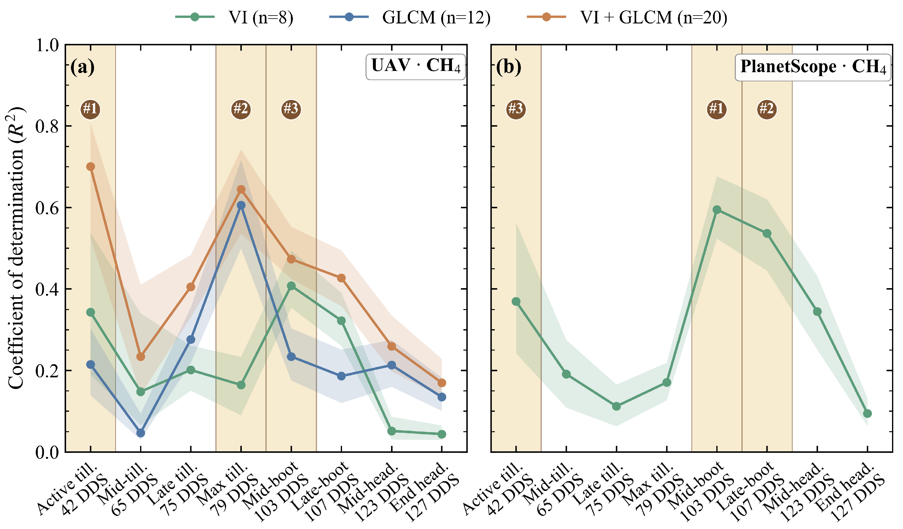
Figure A2.
Median multivariate per phenological stage for N2O. (a) UAV: VI, GLCM and VI + GLCM. (b) PlanetScope: VI only (GLCM not evaluated at 3 m GSD; thermal feature UAV-native, see Section 2.5.2 and Section 2.5.4). Bands: 25–75th bootstrap percentiles per sub-plot.
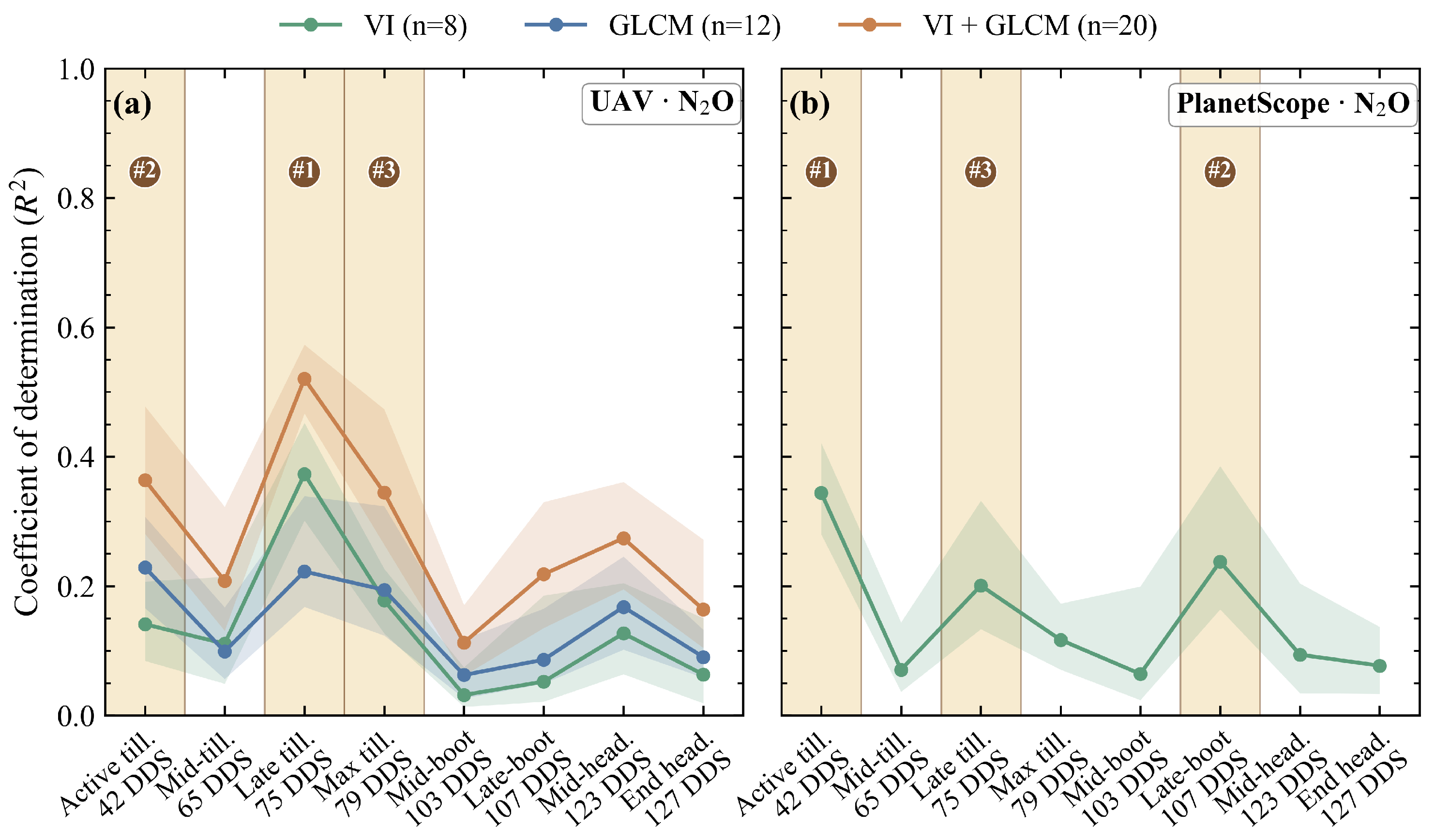
CO2. On UAV (Figure A3a), Maximum tillering stands out for a very strong textural signal: the multivariate GLCM reaches , which evidences that the fine-scale canopy structural heterogeneity captured at ∼4.7 cm/pixel discriminates the net carbon balance better than the VI family alone in that stage; the VI + GLCM combination consolidates the signal at Mid-tillering and Late tillering. On PlanetScope (panel b), the multivariate VI reaches at Late-boot with a more uniform profile across the stages; the satellite predictive ceiling for CO2 is markedly lower than that of the UAV, consistent with the absence of fine-scale textural and thermal descriptors in the native Planet pool.
Figure A3.
Median multivariate per phenological stage for CO2. (a) UAV: VI, GLCM and VI + GLCM. (b) PlanetScope: VI only (GLCM not evaluated at 3 m GSD; thermal feature UAV-native, see Section 2.5.2 and Section 2.5.4). Bands: 25–75th bootstrap percentiles per sub-plot.
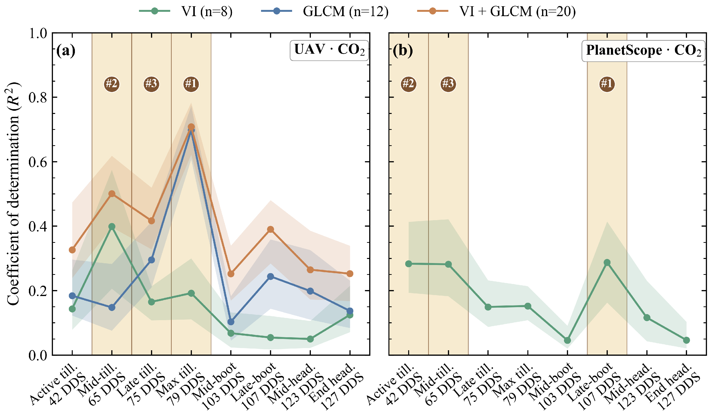
References
- Gao, R.; Zhuo, L.; Duan, Y.; Yan, C.; Yue, Z.; Zhao, Z.; Wu, P. Effects of alternate wetting and drying irrigation on yield, water-saving, and emission reduction in rice fields: A global meta-analysis. Agric. For. Meteorol. 2024, 353, 110075. [Google Scholar] [CrossRef] [Scilit]
- Zhao, C.; Qiu, R.; Zhang, T.; Luo, Y.; Agathokleous, E. Effects of Alternate Wetting and Drying Irrigation on Methane and Nitrous Oxide Emissions From Rice Fields: A Meta-Analysis. Glob. Change Biol. 2024, 30, e17581. [Google Scholar] [CrossRef] [Scilit]
- Adler, P.R.; Nguyen, H.; Rau, B.M.; Dell, C.J. Modeling N2O emissions with remotely sensed variables using machine learning. Environ. Res. Commun. 2024, 6, 091004. [Google Scholar] [CrossRef] [Scilit]
- Gao, T.; Xie, K.; Hu, Q.; Wu, C.; Wang, Z.; Wang, W.; Xiong, D.; Huang, J.; Peng, S.; Cui, K. Alternate wetting and drying irrigation at tillering stage enhances the heat tolerance of rice by increasing sucrose and cytokinin content in panicles. Front. Plant Sci. 2025, 16, 1598652. [Google Scholar] [CrossRef] [Scilit] [PubMed]
- Ramos-Fernández, L.; Gonzales-Quiquia, M.; Huanuqueño-Murillo, J.; Tito-Quispe, D.; Heros-Aguilar, E.; Flores del Pino, L.; Torres-Rua, A. Water Stress Index and Stomatal Conductance under Different Irrigation Regimes with Thermal Sensors in Rice Fields on the Northern Coast of Peru. Remote Sens. 2024, 16, 796. [Google Scholar] [CrossRef] [Scilit]
- Echegaray-Cabrera, I.; Cruz-Villacorta, L.; Ramos-Fernández, L.; Bonilla-Cordova, M.; Heros-Aguilar, E.; Flores del Pino, L. Effect of Alternate Wetting and Drying on the Emission of Greenhouse Gases from Rice Fields on the Northern Coast of Peru. Agronomy 2024, 14, 248. [Google Scholar] [CrossRef] [Scilit]
- Xiao, D.; Ye, C.; Ma, H.; Xu, Y.; Tao, Y.; Zhu, J.; Liao, W.; Chen, S. Soil texture drives rice methane emissions at tillering stage via carbon fractions, nutrients and microbial abundance. J. Integr. Agric. 2025. [Google Scholar] [CrossRef] [Scilit]
- Rehman, T.H.; Lundy, M.E.; Linquist, B.A. Comparative sensitivity of vegetation indices measured via proximal and aerial sensors for assessing N status and predicting grain yield in rice cropping systems. Remote Sens. 2022, 14, 2770. [Google Scholar] [CrossRef] [Scilit]
- Bak, H.J.; Kim, E.J.; Lee, J.H.; Chang, S.; Kwon, D.; Im, W.J.; Kim, D.H.; Lee, I.H.; Lee, M.J.; Hwang, W.H.; et al. Canopy-Level Rice Yield and Yield Component Estimation Using NIR-Based Vegetation Indices. Agriculture 2025, 15, 594. [Google Scholar] [CrossRef] [Scilit]
- Baldin, C.M.; Casella, V.M. Vegetative Index Intercalibration Between PlanetScope and Sentinel-2 Through a SkySat Classification in the Context of “Riserva San Massimo” Rice Farm in Northern Italy. Remote Sens. 2024, 16, 3921. [Google Scholar] [CrossRef] [Scilit]
- Quille-Mamani, J.; Ramos-Fernández, L.; Huanuqueño-Murillo, J.; Quispe-Tito, D.; Cruz-Villacorta, L.; Pino-Vargas, E.; Flores del Pino, L.; Heros-Aguilar, E.; Ángel Ruiz, L. Rice Yield Prediction Using Spectral and Textural Indices Derived from UAV Imagery and Machine Learning Models in Lambayeque, Peru. Remote Sens. 2025, 17, 632. [Google Scholar] [CrossRef] [Scilit]
- Nakano, H.; Tanaka, R.; Guan, S.; Ohdan, H. Predicting rice grain yield using normalized difference vegetation index from UAV and GreenSeeker. Crop Environ. 2023, 2, 59–65. [Google Scholar] [CrossRef] [Scilit]
- Tucker, C.J. Red and photographic infrared linear combinations for monitoring vegetation. Remote Sens. Environ. 1979, 8, 127–150. [Google Scholar] [CrossRef] [Scilit]
- Gitelson, A.A.; Kaufman, Y.J.; Merzlyak, M.N. Use of a green channel in remote sensing of global vegetation from EOS-MODIS. Remote Sens. Environ. 1996, 58, 289–298. [Google Scholar] [CrossRef] [Scilit]
- Rondeaux, G.; Steven, M.; Baret, F. Optimization of soil-adjusted vegetation indices. Remote Sens. Environ. 1996, 55, 95–107. [Google Scholar] [CrossRef] [Scilit]
- Jiang, Z.; Huete, A.R.; Didan, K.; Miura, T. Development of a two-band enhanced vegetation index without a blue band. Remote Sens. Environ. 2008, 112, 3833–3845. [Google Scholar] [CrossRef] [Scilit]
- Sun, X.; Zhang, P.; Wang, Z.; Wang, Y. Potential of multi-seasonal vegetation indices to predict rice yield from UAV multispectral observations. Precis. Agric. 2024, 25, 1235–1261. [Google Scholar] [CrossRef] [Scilit]
- Bascon, M.V.; Nakata, T.; Shibata, S.; Takata, I.; Kobayashi, N.; Kato, Y.; Inoue, S.; Doi, K.; Murase, J.; Nishiuchi, S. Estimating Yield-Related Traits Using UAV-Derived Multispectral Images to Improve Rice Grain Yield Prediction. Agriculture 2022, 12, 1141. [Google Scholar] [CrossRef] [Scilit]
- Su, X.; Wang, J.; Ding, L.; Lu, J.; Zhang, J.; Yao, X.; Cheng, T.; Zhu, Y.; Cao, W.; Tian, Y. Grain yield prediction using multi-temporal UAV-based multispectral vegetation indices and endmember abundance in rice. Field Crops Res. 2023, 299, 108992. [Google Scholar] [CrossRef] [Scilit]
- Haralick, R.M.; Shanmugam, K.; Dinstein, I. Textural Features for Image Classification. IEEE Trans. Syst. Man Cybern. 1973, SMC-3, 610–621. [Google Scholar] [CrossRef] [Scilit]
- Zheng, H.; Cheng, T.; Li, D.; Zhou, X.; Yao, X.; Tian, Y.; Cao, W.; Zhu, Y. Enhancing the nitrogen signals of rice canopies across critical growth stages through the integration of textural and spectral information from UAV-based multispectral imagery. Remote Sens. 2020, 12, 957. [Google Scholar] [CrossRef] [Scilit]
- Liu, J.; Zhu, Y.; Song, L.; Su, X.; Li, J.; Zheng, J.; Zhu, X.; Ren, L.; Wang, W.; Li, X. Optimizing window size and directional parameters of GLCM texture features for estimating rice AGB based on UAVs multispectral imagery. Front. Plant Sci. 2023, 14, 1284235. [Google Scholar] [CrossRef] [Scilit]
- Wang, F.; Yi, Q.; Hu, J.; Xie, L.; Yao, X.; Xu, T.; Zheng, J. Combining spectral and textural information in UAV hyperspectral images to estimate rice grain yield. Int. J. Appl. Earth Obs. Geoinf. 2021, 102, 102397. [Google Scholar] [CrossRef] [Scilit]
- Qiu, Z.; Ma, F.; Li, Z.; Xu, X.; Ge, H.; Du, C. Estimation of nitrogen nutrition index in rice from UAV RGB images coupled with machine learning algorithms. Comput. Electron. Agric. 2021, 189, 106421. [Google Scholar] [CrossRef] [Scilit]
- Ji, S.; Gu, C.; Xi, X.; Zhang, Z.; Hong, Q.; Huo, Z.; Zhao, H.; Zhang, R.; Li, B.; Tan, C. Quantitative Monitoring of Leaf Area Index in Rice Based on Hyperspectral Feature Bands and Ridge Regression Algorithm. Remote Sens. 2022, 14, 2777. [Google Scholar] [CrossRef] [Scilit]
- Li, J.; Cao, Q.; Wang, S.; Li, J.; Zhao, D.; Feng, S.; Cao, Y.; Xu, T. Improved Multi-Stage Rice Above-Ground Biomass Estimation Using Wavelet-Texture-Fused Vegetation Indices from UAV Remote Sensing. Plants 2025, 14, 2903. [Google Scholar] [CrossRef] [Scilit]
- Biswal, S.; Pathak, N.; Chatterjee, C.; Mailapalli, D.R. Estimation of aboveground biomass from spectral and textural characteristics of paddy crop using UAV-multispectral images and machine learning techniques. Geocarto Int. 2024, 39. [Google Scholar] [CrossRef] [Scilit]
- Zeng, Z.C.; Byrne, B.; Gong, F.Y.; He, Z.; Lei, L. Correlation between paddy rice growth and satellite-observed methane column abundance does not imply causation. Nat. Commun. 2021, 12, 1163. [Google Scholar] [CrossRef] [Scilit] [PubMed]
- Yang, Q.; Shi, L.; Han, J.; Chen, Z.; Yu, J. A VI-based phenology adaptation approach for rice crop monitoring using UAV multispectral images. Field Crops Res. 2022, 277, 108419. [Google Scholar] [CrossRef] [Scilit]
- Wang, L.; Chen, S.; Peng, Z.; Huang, J.; Wang, C.; Jiang, H.; Zheng, Q.; Li, D. Phenology Effects on Physically Based Estimation of Paddy Rice Canopy Traits from UAV Hyperspectral Imagery. Remote Sens. 2021, 13, 1792. [Google Scholar] [CrossRef] [Scilit]
- Shrestha, A.; Bheemanahalli, R.; Adeli, A.; Samiappan, S.; Czarnecki, J.M.P.; McCraine, C.D.; Reddy, K.R.; Moorhead, R.J. Phenological stage and vegetation index for predicting corn yield under rainfed environments. Front. Plant Sci. 2023, 14, 1168732. [Google Scholar] [CrossRef] [Scilit]
- Dai, Q.; Chen, H.; Chen, Z.; Liu, C.; Li, G.; Wang, Y. Identification of optimal phenological periods for summer maize yield prediction using UAV-based multispectral data. J. Integr. Agric. 2025. [Google Scholar] [CrossRef] [Scilit]
- Carracelas, G.; Hornbuckle, J.; Ballester, C. Monitoring Nitrogen Uptake and Grain Quality in Ponded and Aerobic Rice with the Squared Simplified Canopy Chlorophyll Content Index. Remote Sens. 2025, 17, 2598. [Google Scholar] [CrossRef] [Scilit]
- Khose, S.B.; Mailapalli, D.R. UAV-based multispectral image analytics and machine learning for predicting crop nitrogen in rice. Geocarto Int. 2024, 39. [Google Scholar] [CrossRef] [Scilit]
- Ibrahim, S.; Balzter, H.; Ozigis, M.S. Estimating paddy rice yield using PlanetScope imagery and machine learning. Smart Agric. Technol. 2025, 12, 101447. [Google Scholar] [CrossRef] [Scilit]
- Swain, K.C.; Singha, C.; Pradhan, B. Estimating Total Rice Biomass and Crop Yield at Field Scale Using PlanetScope Imagery Through Hybrid Machine Learning Models. Earth Syst. Environ. 2024, 8, 1713–1731. [Google Scholar] [CrossRef] [Scilit]
- Chen, T.; Guestrin, C. XGBoost: A Scalable Tree Boosting System. In Proceedings of the 22nd ACM SIGKDD International Conference on Knowledge Discovery and Data Mining, San Francisco, CA, USA, 13–17 August 2016; pp. 785–794. [Google Scholar] [CrossRef] [Scilit]
- Velez, A.F.; Alvarez, C.I.; Navarro, F.; Guzman, D.; Bohorquez, M.P.; Selvaraj, M.G.; Ishitani, M. Assessing methane emissions from paddy fields through environmental and UAV remote sensing variables. Environ. Monit. Assess. 2024, 196, 574. [Google Scholar] [CrossRef] [Scilit] [PubMed]
- Wu, Q.; Wang, J.; He, Y.; Liu, Y.; Jiang, Q. Quantitative assessment and mitigation strategies of greenhouse gas emissions from rice fields in China: A data-driven approach based on machine learning and statistical modeling. Comput. Electron. Agric. 2023, 210, 107929. [Google Scholar] [CrossRef] [Scilit]
- Jiang, Z.; Yang, S.; Smith, P.; Pang, Q. Ensemble machine learning for modeling greenhouse gas emissions at different time scales from irrigated paddy fields. Field Crops Res. 2023, 292, 108821. [Google Scholar] [CrossRef] [Scilit]
- Killeen, P.; Kiringa, I.; Yeap, T.; Branco, P. Corn grain yield prediction using UAV-based high spatio-temporal resolution imagery, machine learning, and spatial cross-validation. Remote Sens. 2024, 16, 683. [Google Scholar] [CrossRef] [Scilit]
- Stiller, S.; Grahmann, K.; Ghazaryan, G.; Ryo, M. Improving spatial transferability of deep learning models for small-field crop yield prediction. Isprs Open J. Photogramm. Remote Sens. 2024, 12, 100064. [Google Scholar] [CrossRef] [Scilit]
- Habibi, L.N.; Matsui, T.; Tanaka, T.S. Critical evaluation of the effects of a cross-validation strategy and machine learning optimization on the prediction accuracy and transferability of a soybean yield prediction model using UAV-based remote sensing. J. Agric. Food Res. 2024, 16, 101096. [Google Scholar] [CrossRef] [Scilit]
- Dinh, T.L.A.; Aires, F. Nested leave-two-out cross-validation for the optimal crop yield model selection. Geosci. Model Dev. 2022, 15, 3519–3535. [Google Scholar] [CrossRef] [Scilit]
- Hutchinson, G.L.; Mosier, A.R. Improved Soil Cover Method for Field Measurement of Nitrous Oxide Fluxes. Soil Sci. Soc. Am. J. 1981, 45, 311–316. [Google Scholar] [CrossRef] [Scilit]
- Venterea, R.T.; Petersen, S.O.; de Klein, C.A.M.; Pedersen, A.R.; Noble, A.D.L.; Rees, R.M.; Gamble, J.D.; Parkin, T.B. Global Research Alliance N2O chamber methodology guidelines: Flux calculations. J. Environ. Qual. 2020, 49, 1141–1155. [Google Scholar] [CrossRef] [Scilit]
- Lombardi, B.; Loaiza, S.; Trujillo, C.; Arevalo, A.; Vázquez, E.; Arango, J.; Chirinda, N. Greenhouse gas emissions from cattle dung depositions in two Urochloa forage fields with contrasting biological nitrification inhibition (BNI) capacity. Geoderma 2022, 406, 115516. [Google Scholar] [CrossRef] [Scilit] [PubMed]
- Lawrence, N.C.; Hall, S.J. Capturing temporal heterogeneity in soil nitrous oxide fluxes with a robust and low-cost automated chamber apparatus. Atmos. Meas. Tech. 2020, 13, 4065–4078. [Google Scholar] [CrossRef] [Scilit]
- Yue, H.; Liu, C.; Zhang, W.; Dannenmann, M.; Wang, X.; Yao, Z.; Song, C.; Butterbach-Bahl, K. How to Improve Cumulative Methane and Nitrous Oxide Flux Estimations of the Non-Steady-State Chamber Method? J. Geophys. Res. Biogeosciences 2022, 127, e2021JG006641. [Google Scholar] [CrossRef] [Scilit]
- Meier, U. Growth stages of mono- and dicotyledonous plants: BBCH Monograph, 2nd ed.; Federal Biological Research Centre for Agriculture and Forestry: Berlin, Germany; Braunschweig, Germany, 2001. [Google Scholar] [CrossRef]
- Huang, H.; Roy, D.P. Characterization of PlanetScope-0 PlanetScope-1 surface reflectance and normalized difference vegetation index continuity. Sci. Remote Sens. 2021, 3, 100014. [Google Scholar] [CrossRef] [Scilit]
- Jiang, J.; Johansen, K.; Tu, Y.H.; McCabe, M.F. Multi-sensor and multi-platform consistency and interoperability between UAV, Planet CubeSat, Sentinel-2, and Landsat reflectance data. Giscience Remote Sens. 2022, 59, 936–958. [Google Scholar] [CrossRef] [Scilit]
- Ma, Y.; Li, W.; Wang, J.; Liu, S.; Dong, M.; Shi, Z. Evaluating the consistency between Sentinel-2 and Planet constellations at field scale: Illustration over winter wheat. Precis. Agric. 2025, 26, 31. [Google Scholar] [CrossRef] [Scilit]
- Vanhellemont, Q. Evaluation of eight band SuperDove imagery for aquatic applications. Opt. Express 2023, 31, 13851. [Google Scholar] [CrossRef] [Scilit]
- Baldin, C.M.; Casella, V.M. Comparison of PlanetScope and Sentinel-2 Spectral Channels and Their Alignment via Linear Regression for Enhanced Index Derivation. Geosciences 2025, 15, 184. [Google Scholar] [CrossRef] [Scilit]
- Gitelson, A.A.; Gritz, Y.; Merzlyak, M.N. Relationships between leaf chlorophyll content and spectral reflectance and algorithms for non-destructive chlorophyll assessment in higher plant leaves. J. Plant Physiol. 2003, 160, 271–282. [Google Scholar] [CrossRef] [Scilit] [PubMed]
- McFeeters, S.K. The use of the Normalized Difference Water Index (NDWI) in the delineation of open water features. Int. J. Remote Sens. 1996, 17, 1425–1432. [Google Scholar] [CrossRef] [Scilit]
- Dormann, C.F.; Elith, J.; Bacher, S.; Buchmann, C.; Carl, G.; Carré, G.; Marquéz, J.R.G.; Gruber, B.; Lafourcade, B.; Leitão, P.J.; et al. Collinearity: A review of methods to deal with it and a simulation study evaluating their performance. Ecography 2013, 36, 27–46. [Google Scholar] [CrossRef] [Scilit]
- Marino, S.; Alvino, A. Vegetation Indices Data Clustering for Dynamic Monitoring and Classification of Wheat Yield Crop Traits. Remote Sens. 2021, 13, 541. [Google Scholar] [CrossRef] [Scilit]
- Hall-Beyer, M. Practical guidelines for choosing GLCM textures to use in landscape classification tasks over a range of moderate spatial scales. Int. J. Remote Sens. 2017, 38, 1312–1338. [Google Scholar] [CrossRef] [Scilit]
- Liu, Y.; Feng, H.; Yue, J.; Jin, X.; Li, Z.; Yang, G. Estimation of potato above-ground biomass based on unmanned aerial vehicle red-green-blue images with different texture features and crop height. Front. Plant Sci. 2022, 13. [Google Scholar] [CrossRef] [Scilit]
- Xu, L.; Zhou, L.; Meng, R.; Zhao, F.; Lv, Z.; Xu, B.; Zeng, L.; Yu, X.; Peng, S. An improved approach to estimate ratoon rice aboveground biomass by integrating UAV-based spectral, textural and structural features. Precis. Agric. 2022, 23, 1276–1301. [Google Scholar] [CrossRef] [Scilit]
- Xu, J.; Lv, Y.; Liu, X.; Dalson, T.; Yang, S.; Wu, J. Diagnosing Crop Water Stress of Rice using Infra-red Thermal Imager under Water Deficit Condition. Int. J. Agric. Biol. 2016, 18, 565–572. [Google Scholar] [CrossRef] [Scilit]
- Bian, J.; Zhang, Z.; Chen, J.; Chen, H.; Cui, C.; Li, X.; Chen, S.; Fu, Q. Simplified evaluation of cotton water stress using high-resolution UAV thermal imagery. Remote Sens. 2019, 11, 267. [Google Scholar] [CrossRef] [Scilit]
- Kapari, M.; Sibanda, M.; Magidi, J.; Mabhaudhi, T.; Nhamo, L.; Mpandeli, S. Comparing Machine Learning Algorithms for Estimating the Maize Crop Water Stress Index (CWSI) Using UAV-Acquired Remotely Sensed Data in Smallholder Croplands. Drones 2024, 8, 61. [Google Scholar] [CrossRef] [Scilit]
- Varma, S.; Simon, R. Bias in error estimation when using cross-validation for model selection. Bmc Bioinform. 2006, 7, 91. [Google Scholar] [CrossRef] [Scilit]
- Roberts, D.R.; Bahn, V.; Ciuti, S.; Boyce, M.S.; Elith, J.; Guillera-Arroita, G.; Hauenstein, S.; Lahoz-Monfort, J.J.; Schröder, B.; Thuiller, W.; et al. Cross-validation strategies for data with temporal, spatial, hierarchical, or phylogenetic structure. Ecography 2017, 40, 913–929. [Google Scholar] [CrossRef] [Scilit]
- Breiman, L. Random Forests. Mach. Learn. 2001, 45, 5–32. [Google Scholar] [CrossRef] [Scilit]
- Hurlbert, S.H. Pseudoreplication and the Design of Ecological Field Experiments. Ecol. Monogr. 1984, 54, 187–211. [Google Scholar] [CrossRef] [Scilit]
- Yoo, M.; Koo, H. Exploring the impact of spatial autocorrelation on optimistic bias in cross-validation and assessing the effectiveness of spatial cross-validation. Cartogr. Geogr. Inf. Sci. 2024, 52, 596–609. [Google Scholar] [CrossRef] [Scilit]
- Pedregosa, F.; Varoquaux, G.; Gramfort, A.; Michel, V.; Thirion, B.; Grisel, O.; Blondel, M.; Prettenhofer, P.; Weiss, R.; Dubourg, V.; et al. Scikit-learn: Machine Learning in Python. J. Mach. Learn. Res. 2011, 12, 2825–2830. [Google Scholar]
- Ojala, M.; Garriga, G.C. Permutation Tests for Studying Classifier Performance. In Proceedings of the 2009 Ninth IEEE International Conference on Data Mining, Miami, FL, USA, 6–9 December 2009; pp. 908–913. [Google Scholar] [CrossRef] [Scilit]
- Matthews, K.E.; Facelli, J.M.; Cavagnaro, T.R. Response of soil microbial community structure, carbon and nitrogen cycling to drying and rewetting. Appl. Soil Ecol. 2023, 192, 105099. [Google Scholar] [CrossRef] [Scilit]
- Lampayan, R.M.; Rejesus, R.M.; Singleton, G.R.; Bouman, B.A.M. Adoption and economics of alternate wetting and drying water management for irrigated lowland rice. Field Crops Res. 2015, 170, 95–108. [Google Scholar] [CrossRef] [Scilit]
- Bouman, B.A.M.; Tuong, T.P. Field water management to save water and increase its productivity in irrigated lowland rice. Agric. Water Manag. 2001, 49, 11–30. [Google Scholar] [CrossRef] [Scilit]
- Wan, L.; Cen, H.; Zhu, J.; Zhang, J.; Zhu, Y.; He, Y. Grain yield prediction of rice using multi-temporal UAV-based RGB and multispectral images and model transfer—A case study of small farmlands in the South of China. Agric. For. Meteorol. 2020, 291, 108096. [Google Scholar] [CrossRef] [Scilit]
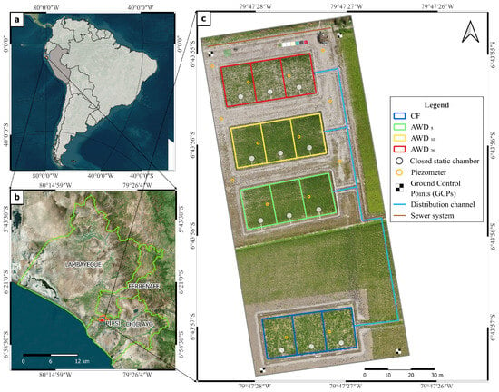
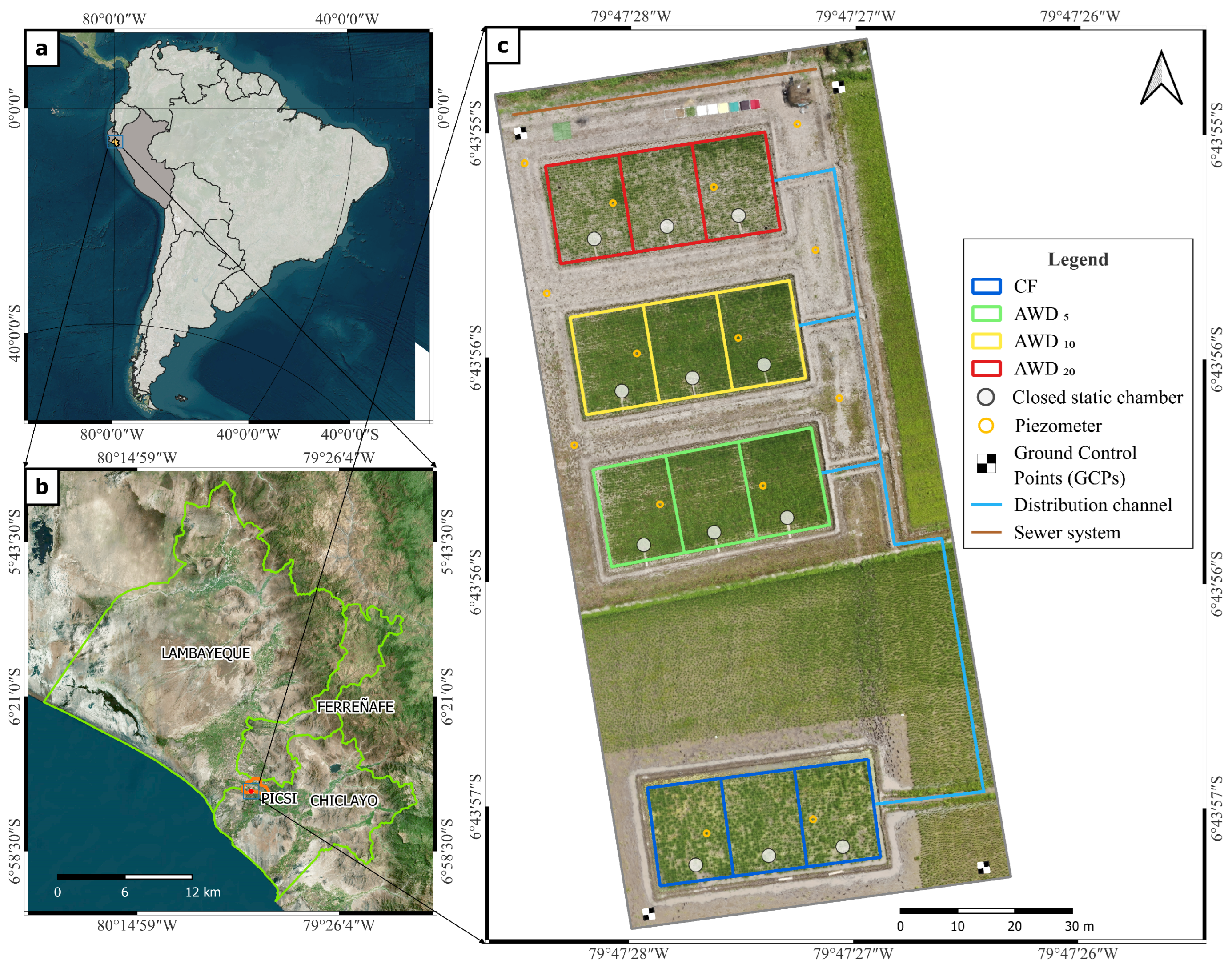
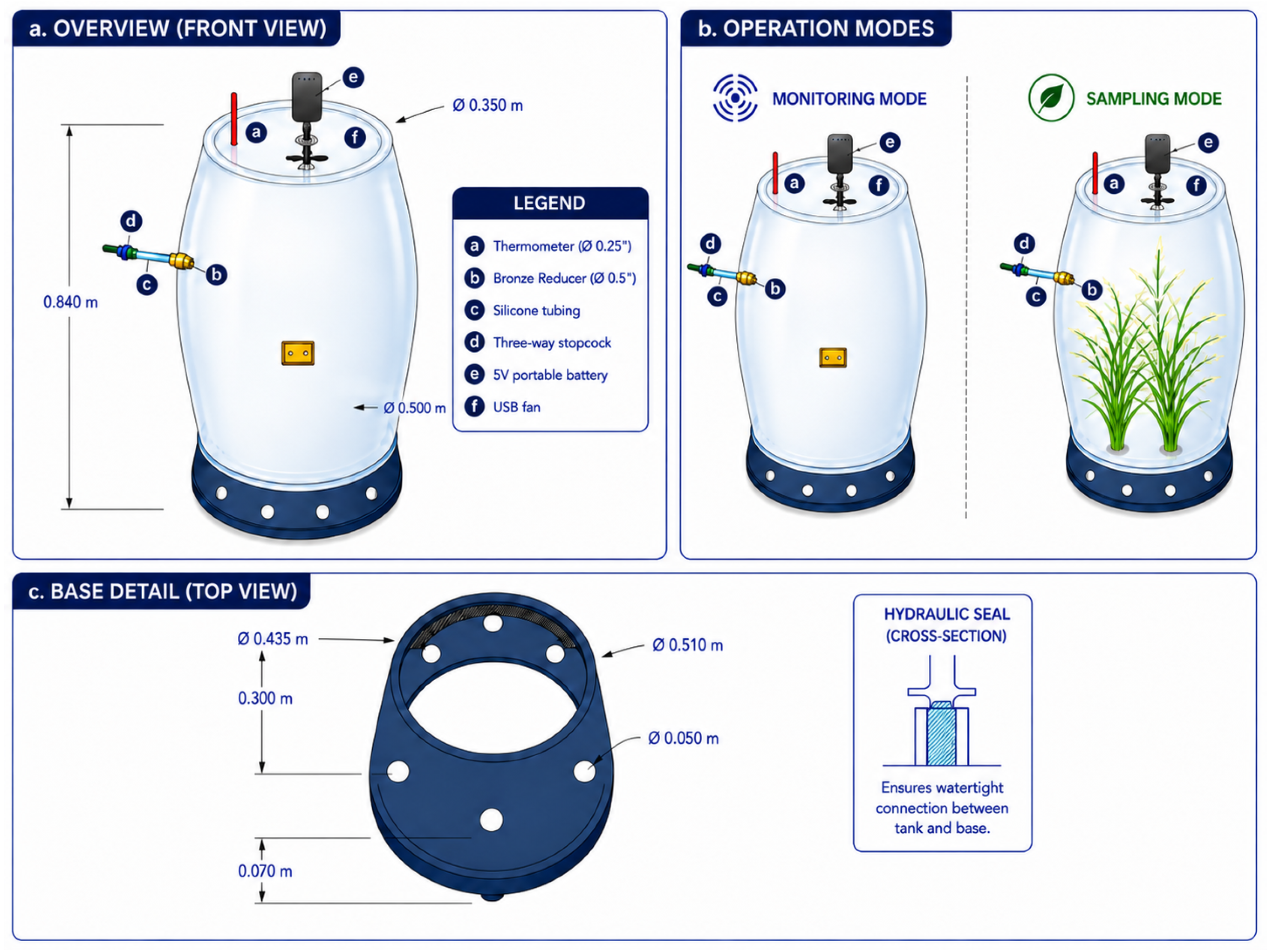
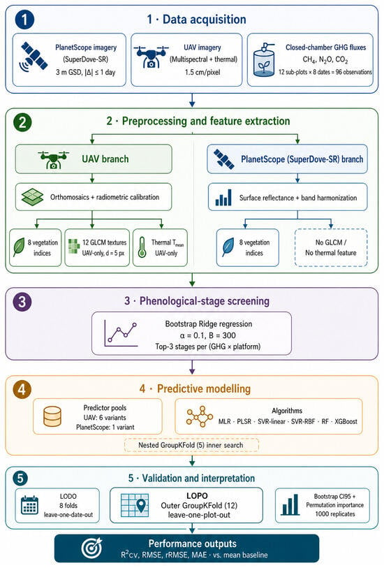
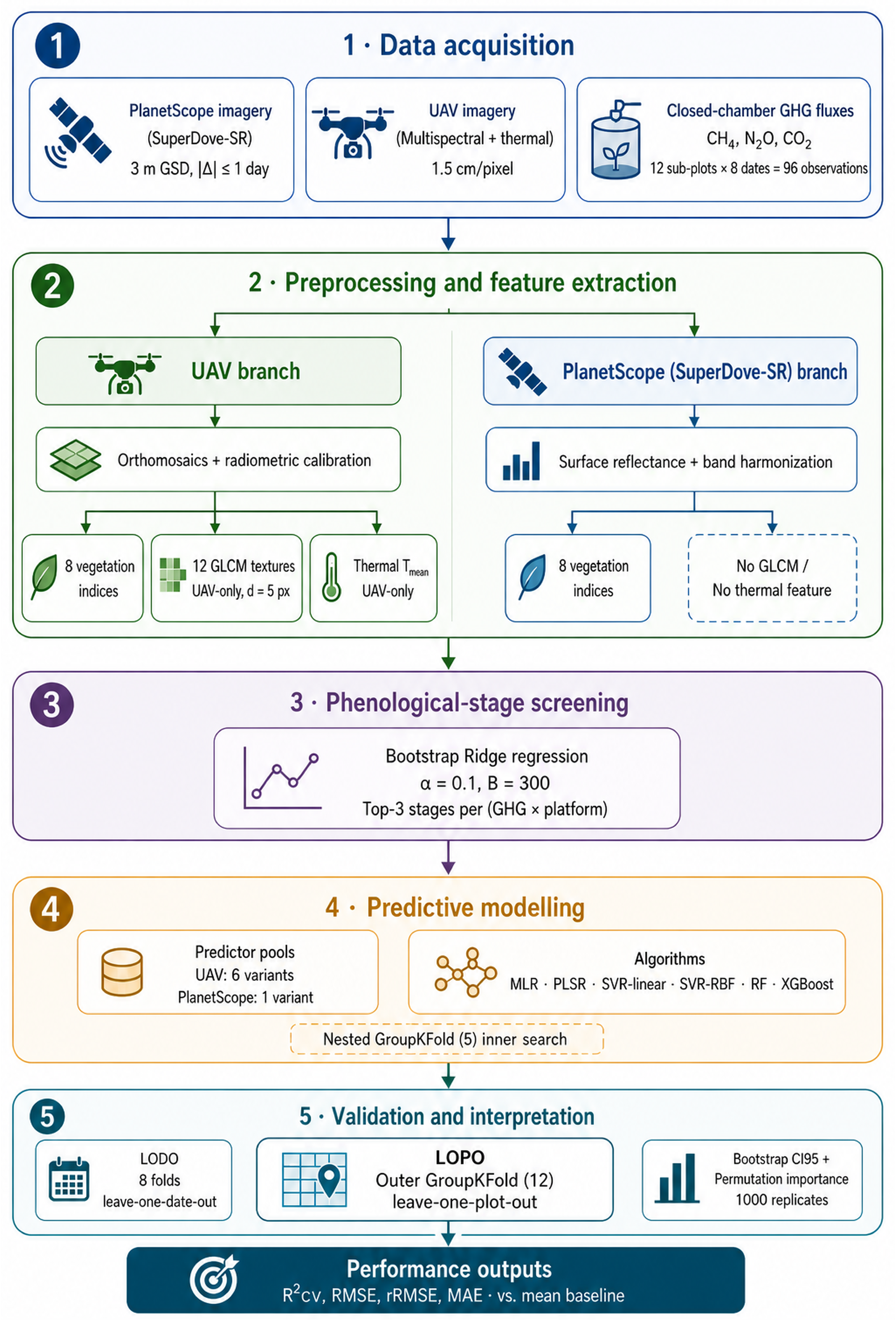
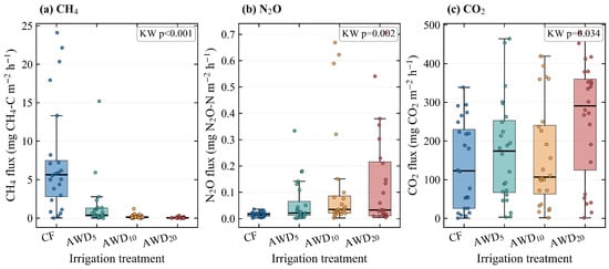
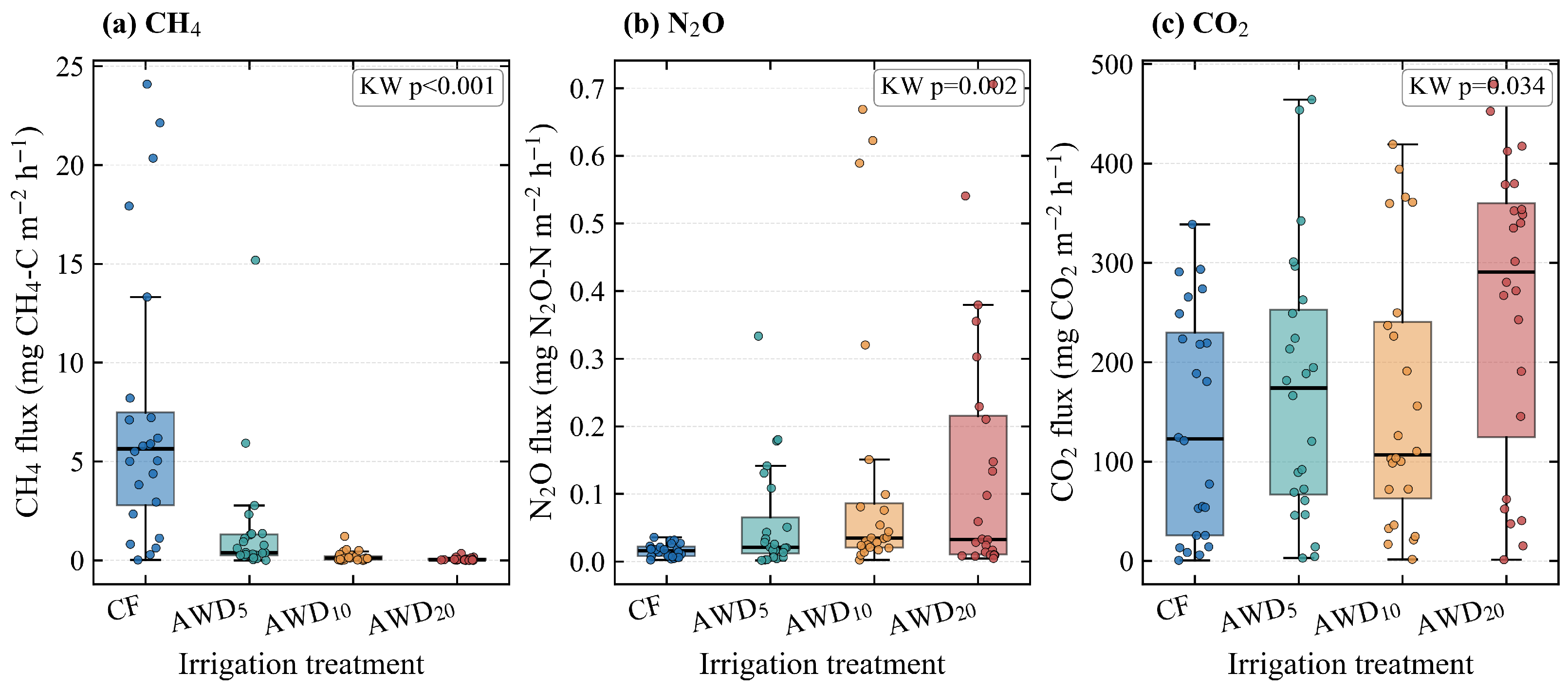
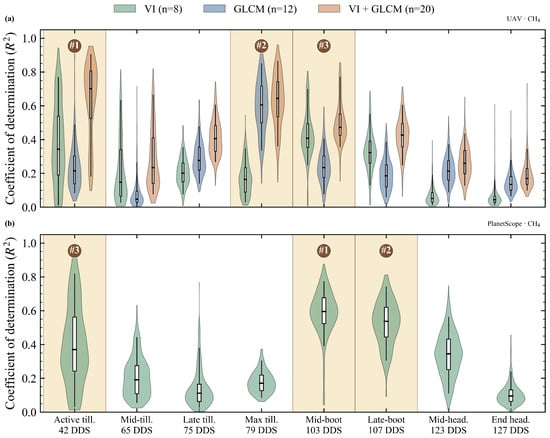
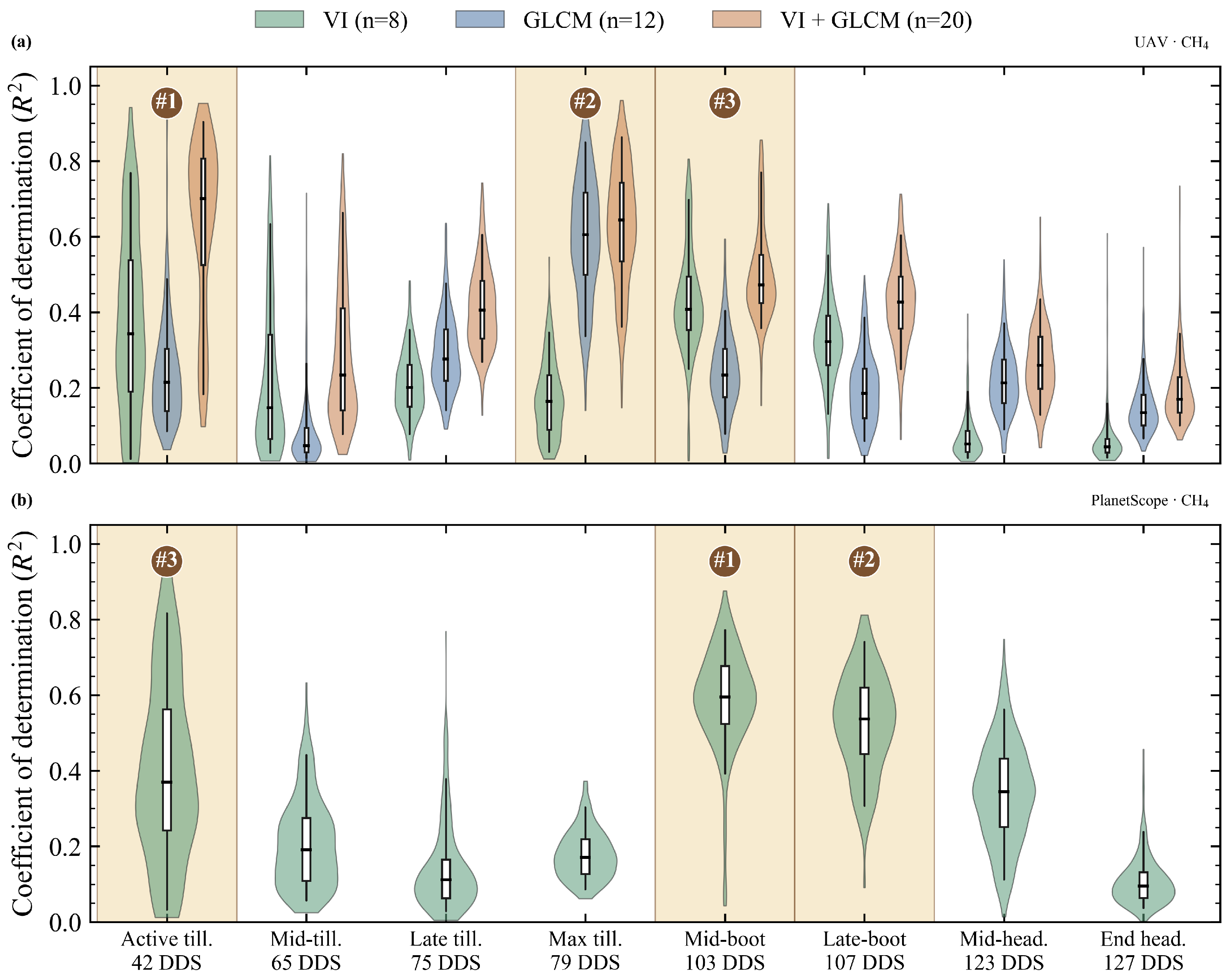
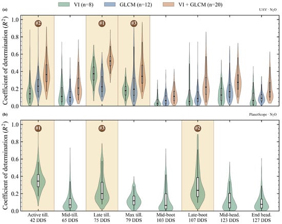
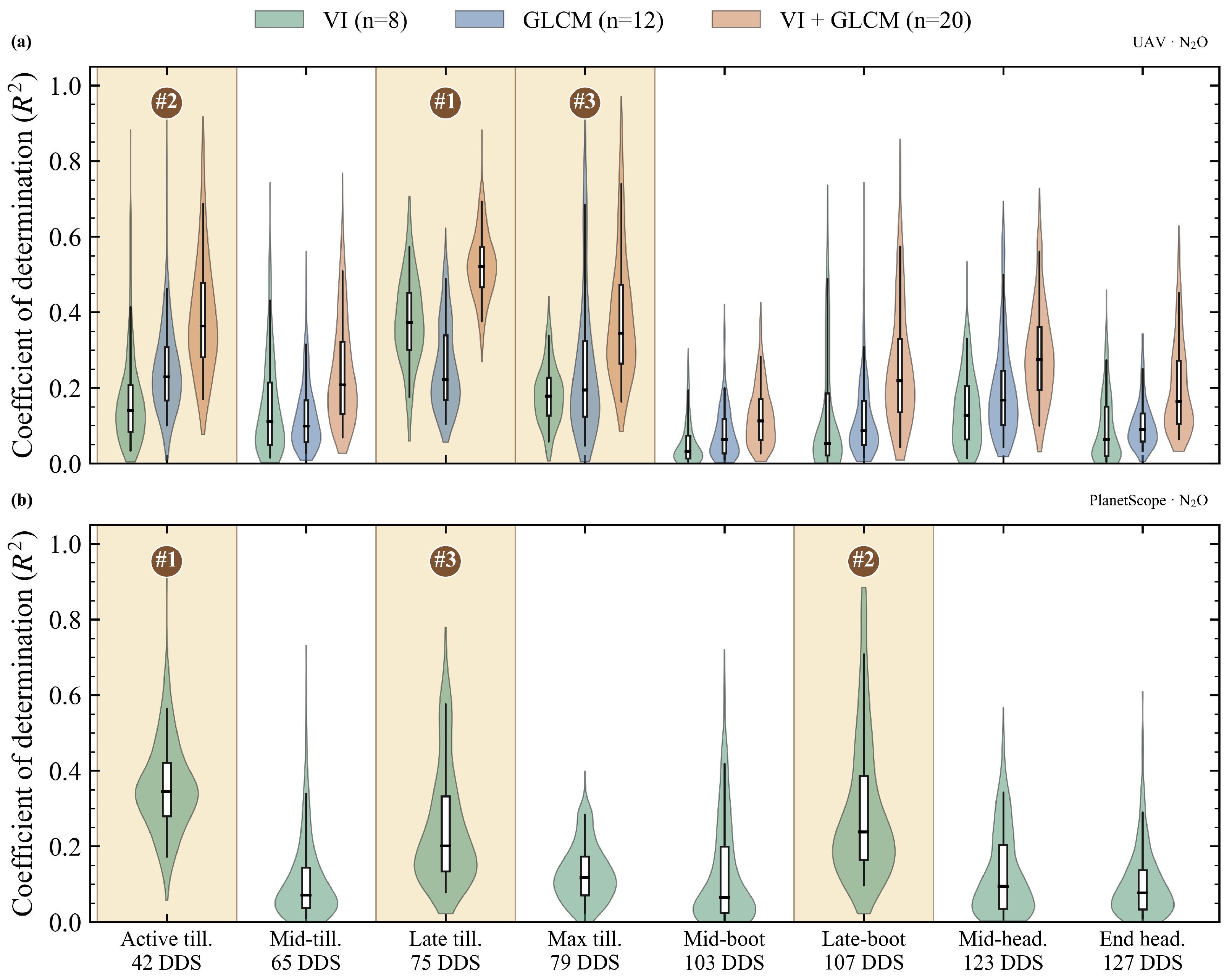
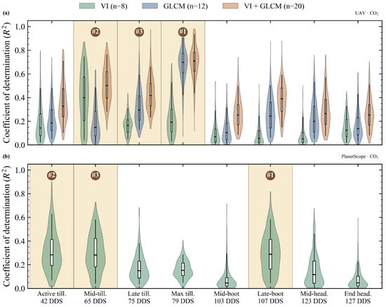
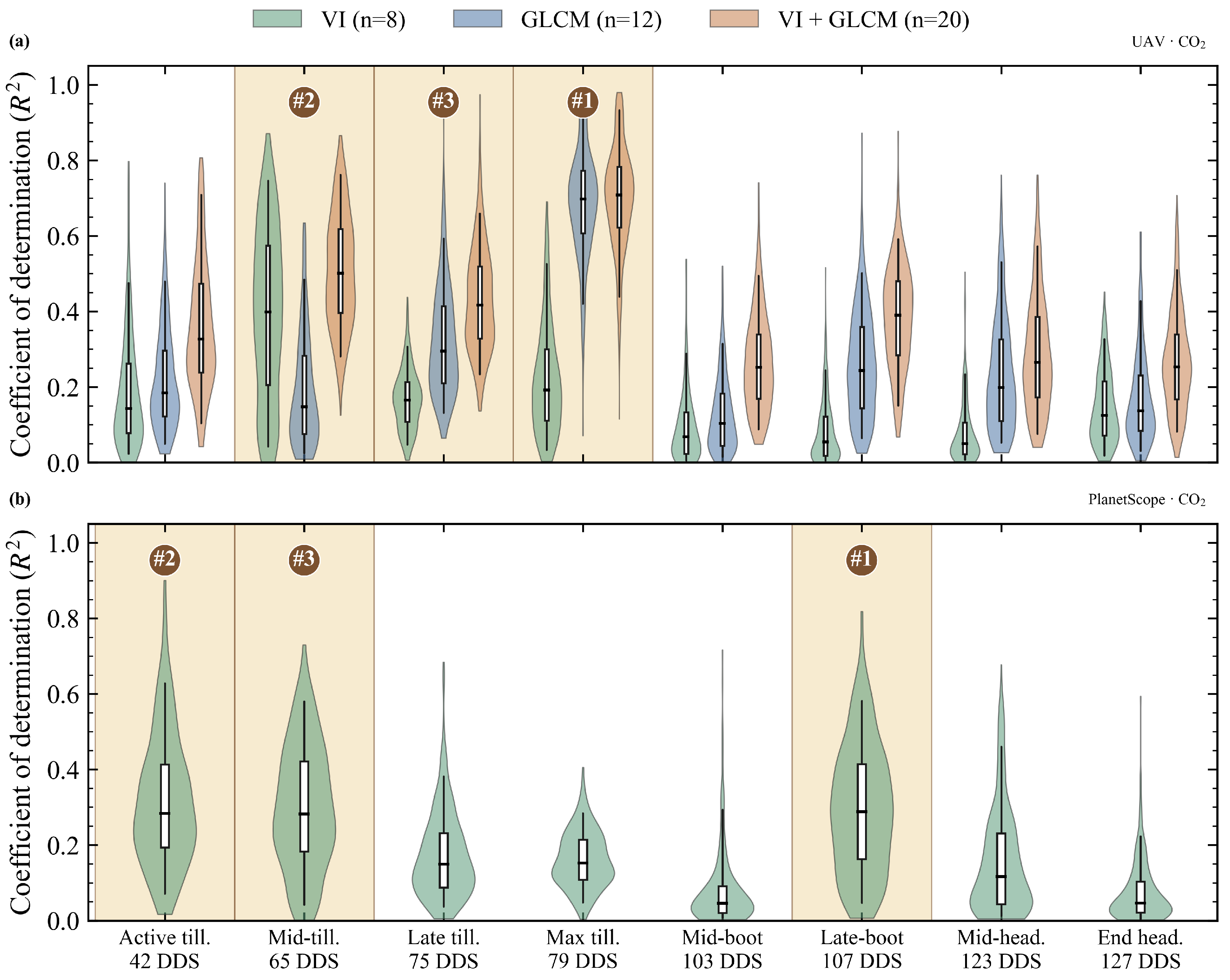
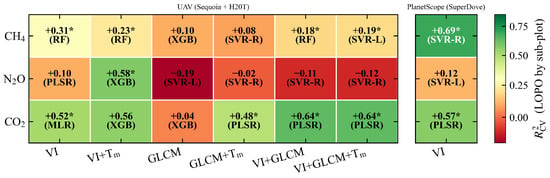
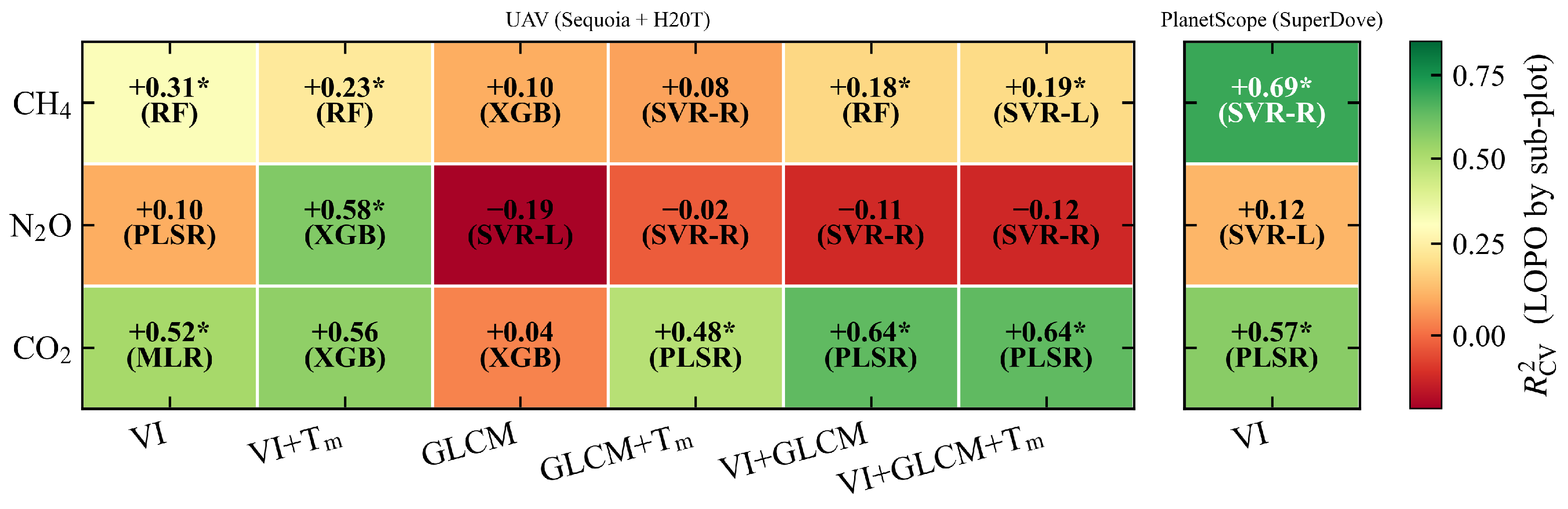
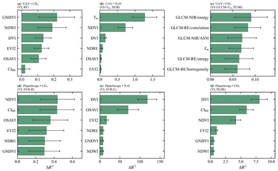
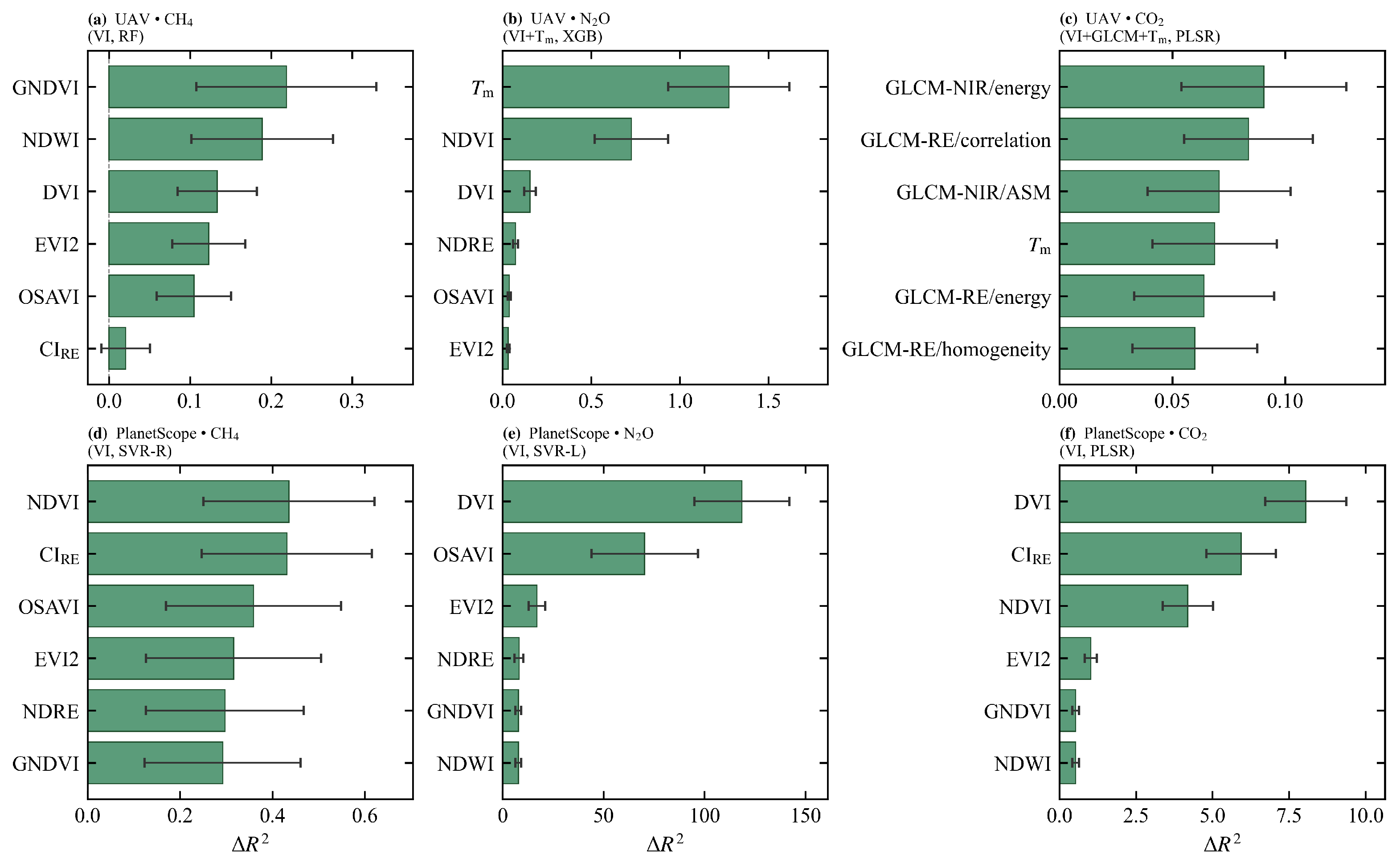
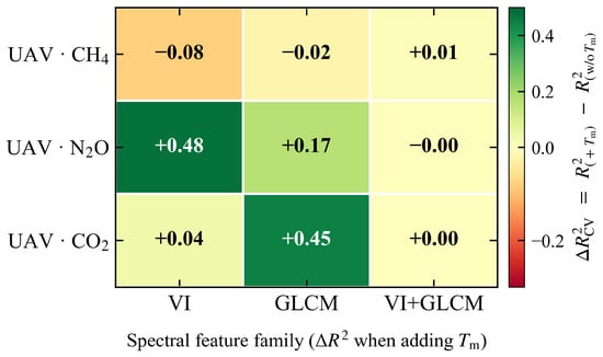
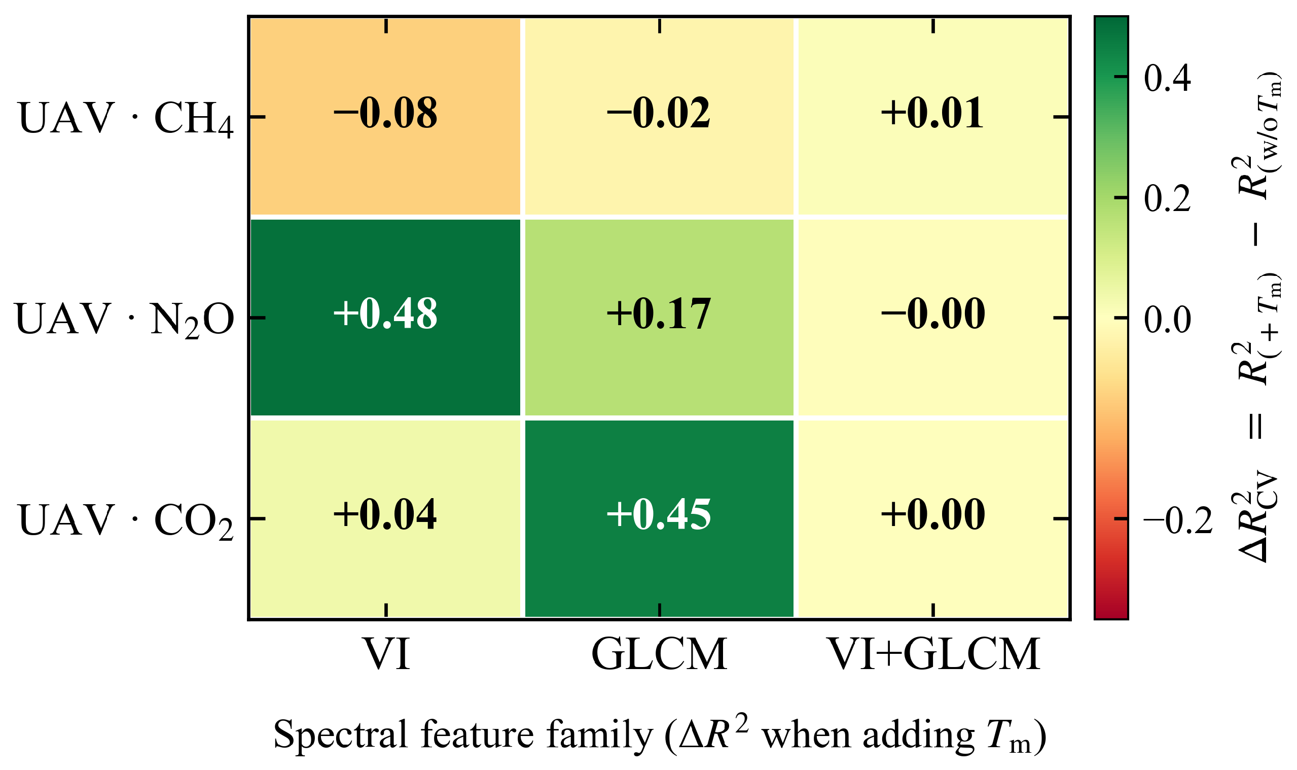
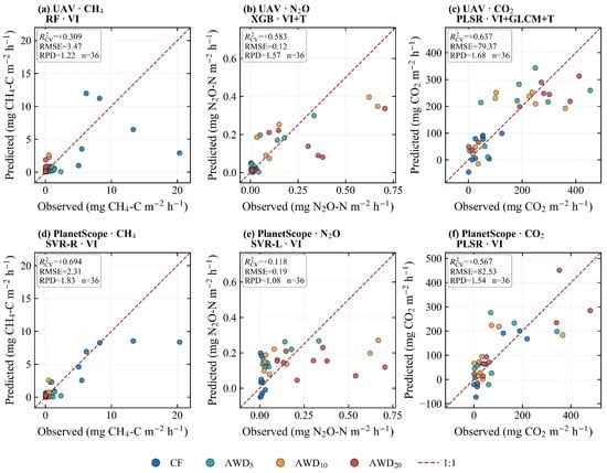
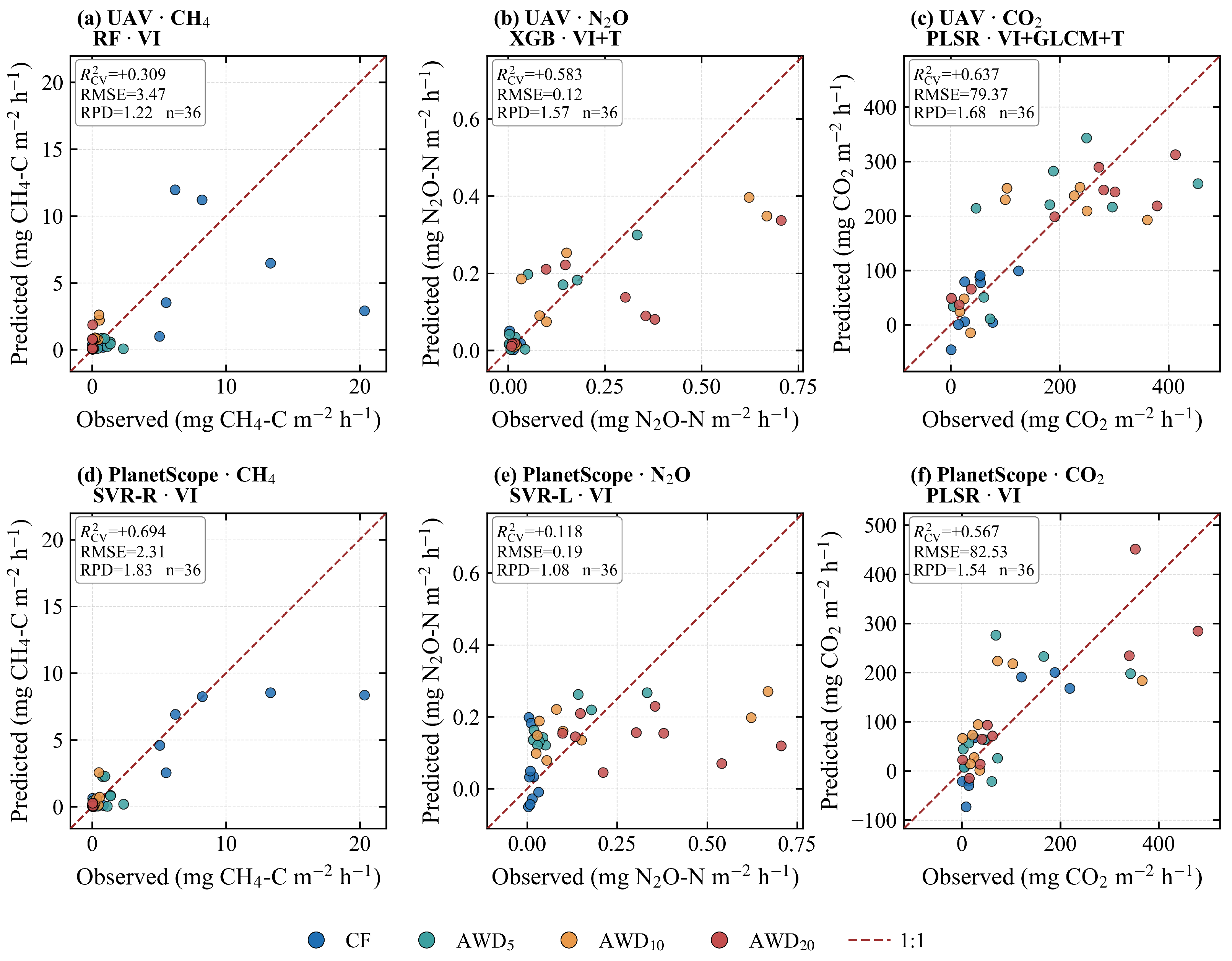

Disclaimer/Publisher’s Note: The statements, opinions and data contained in all publications are solely those of the individual author(s) and contributor(s) and not of MDPI and/or the editor(s). MDPI and/or the editor(s) disclaim responsibility for any injury to people or property resulting from any ideas, methods, instructions or products referred to in the content. |
© 2026 by the authors. Licensee MDPI, Basel, Switzerland. This article is an open access article distributed under the terms and conditions of the Creative Commons Attribution (CC BY) license.