Extraction of Detailed 3D Coseismic Displacements in the 2024 Noto Peninsula Earthquake from Airborne LiDAR Data

Highlights

What are the main findings?

• Detailed three-dimensional (3D) coseismic ground-surface displacements associated with the 2024 Noto Peninsula earthquake were derived from airborne LiDAR data using the Iterative Closest Point (ICP) method with a moving-window technique.
• The derived ground-surface displacements were validated against 59 GNSS observations, achieving high accuracy with a root mean square error (RMSE) of less than 0.2 m.

What are the implications of the main findings?

• Pre- and post-event high-density airborne LiDAR data are effective for estimating coseismic displacements, bridging wide-area deformation derived from satellite SAR data and point-based displacements measured by GNSS observations.
• Ground-surface displacements consist of two components: coseismic crustal deformation and local displacements caused by ground failures.

Abstract

Airborne LiDAR data acquired before and after the 2024 Noto Peninsula earthquake in Japan were used to estimate three-dimensional (3D) ground-surface displacements based on the Iterative Closest Point (ICP) algorithm. Digital elevation (terrain) models (DEMs) were generated from pre-earthquake point cloud data acquired by Ishikawa Prefecture and compared with post-earthquake DEMs developed by the Forestry Agency of Japan. Three-dimensional coseismic displacements were derived from the spatial correlations between pre- and post-event DEMs for 50 m × 50 m tiles. The results depend on the tile size and are influenced by ground movements within and surrounding each tile. Therefore, moving-average windows of 250 m and 550 m were applied to the 50 m tiles to obtain continuous 3D displacement fields across the ground surface. A comparison between GNSS-measured displacements and the corresponding moving-average estimates for tiles containing triangulation points and continuously operating reference stations (CORSs) showed that the accuracy of the estimated displacements in all three components was within 0.2 m in terms of the root mean square error (RMSE).

1. Introduction

At 07:10 UTC on 1 January 2024, a moment magnitude (Mw) 7.5 earthquake occurred near the northeastern tip of the Noto Peninsula in Central Japan [1,2,3]. The earthquake caused significant crustal deformation across the entire peninsula, with the seafloor emerging above sea level over a wide area along the northern coast [4,5]. Seismic waveforms and permanent displacements [6,7], together with tsunami waveforms [8,9] and tsunami run-up heights [10], provide fundamental information for constructing earthquake source-fault models. Regional crustal deformation and localized ground failures both contribute to the three-dimensional (3D) displacement of the ground surface. Earthquake-induced crustal deformation also changes the positions of surveying reference points, such as triangulation and leveling points [11], and can shift road and residential boundary lines [12]. Because remeasuring these survey reference points takes time, about 1300 real-time electronic reference stations (GEONET) based on satellite positioning (GNSS) had already been deployed throughout Japan [13]. However, only six or seven stations were placed in the northern Noto region [14,15]. Temporary GNSS stations had also been installed by universities after the active swarm that began in November 2020 near the northeastern tip of the peninsula (Suzu City) [16,17], and additional stations were operated by SoftBank Corp. [17,18], but these datasets were not openly available.

Evaluating crustal deformation is a major challenge in assessing the impact of the 2024 Noto Peninsula earthquake. Wide-area estimates have been obtained using differential interferometric SAR (DInSAR) and pixel-offset (tracking) analyses of satellite SAR data [7,17,19]. However, the coherence was low because of severe ground failures in the northern peninsula, and phase-unwrapped satellite line-of-sight (LOS) displacements could not be obtained from the DInSAR analyses. A three-dimensional topographic differencing (3DTD) analysis using airborne LiDAR data has also been reported [20], but further verification is still needed. Coseismic displacements at strong-motion observation points can also be calculated by integrating seismometer records [21,22], but the observation network on the Noto Peninsula was not dense enough to estimate the detailed distribution of crustal deformation.

In the Wajima and Suzu cities in the northern Noto Peninsula, where crustal deformation was large and slope failures were frequent, surveying control points such as triangulation and leveling points remained infeasible for an extended period after the earthquake [23]. However, after the on-site conditions had been confirmed and GNSS observations had been completed, the triangulation points in the northern peninsula resumed their role as surveying control points at the end of May 2025 [23]. In this study, some of the GNSS survey results obtained before and after the earthquake at 154 surveying control points in the Northern Noto region, provided by the Geospatial Information Authority of Japan (GSI), are used as reference data for the crustal deformation caused by the earthquake.

This study aims to derive detailed, continuous 3D ground-surface displacements from pre- and post-earthquake airborne LiDAR data, thereby linking GNSS observations at survey control points with wide-area satellite-image analysis results. Using point-cloud data from pre-earthquake airborne LiDAR measurements conducted by Ishikawa Prefecture [24] and digital elevation models (DEMs) from post-earthquake airborne LiDAR data compiled by the Forestry Agency of Japan [25], we perform a 3D topographic differencing (3DTD) analysis based on the Iterative Closest Point (ICP) algorithm [26,27,28]. Because the pre- and post-earthquake DEMs are generated and compared on 0.5 m grids, this method is expected to provide horizontal accuracy of a fraction of the grid spacing [29,30,31]. However, because the results of the ICP method depend on the size and arrangement of the calculation window (tile), this study proposes a moving-average method using a window whose side length is an odd-number multiple of the 50 m square tile, which is considered sufficiently small for ICP analysis.

In this study, we also attempt to separate ground-surface displacement into two components: crustal movement and local soil movement. The moving-average results are compared with GNSS observations at survey control points (triangulation points and GEONET stations) to verify the broad-area coverage and accurate 3D crustal deformation in the northern Noto Peninsula caused by the 2024 earthquake.

2. Materials and Methods

2.1. The 2024 Noto Peninsula Earthquake and Crustal Deformation

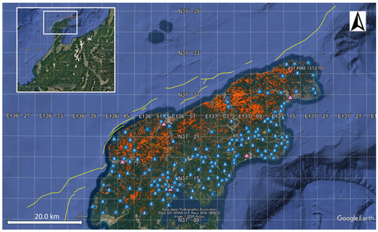
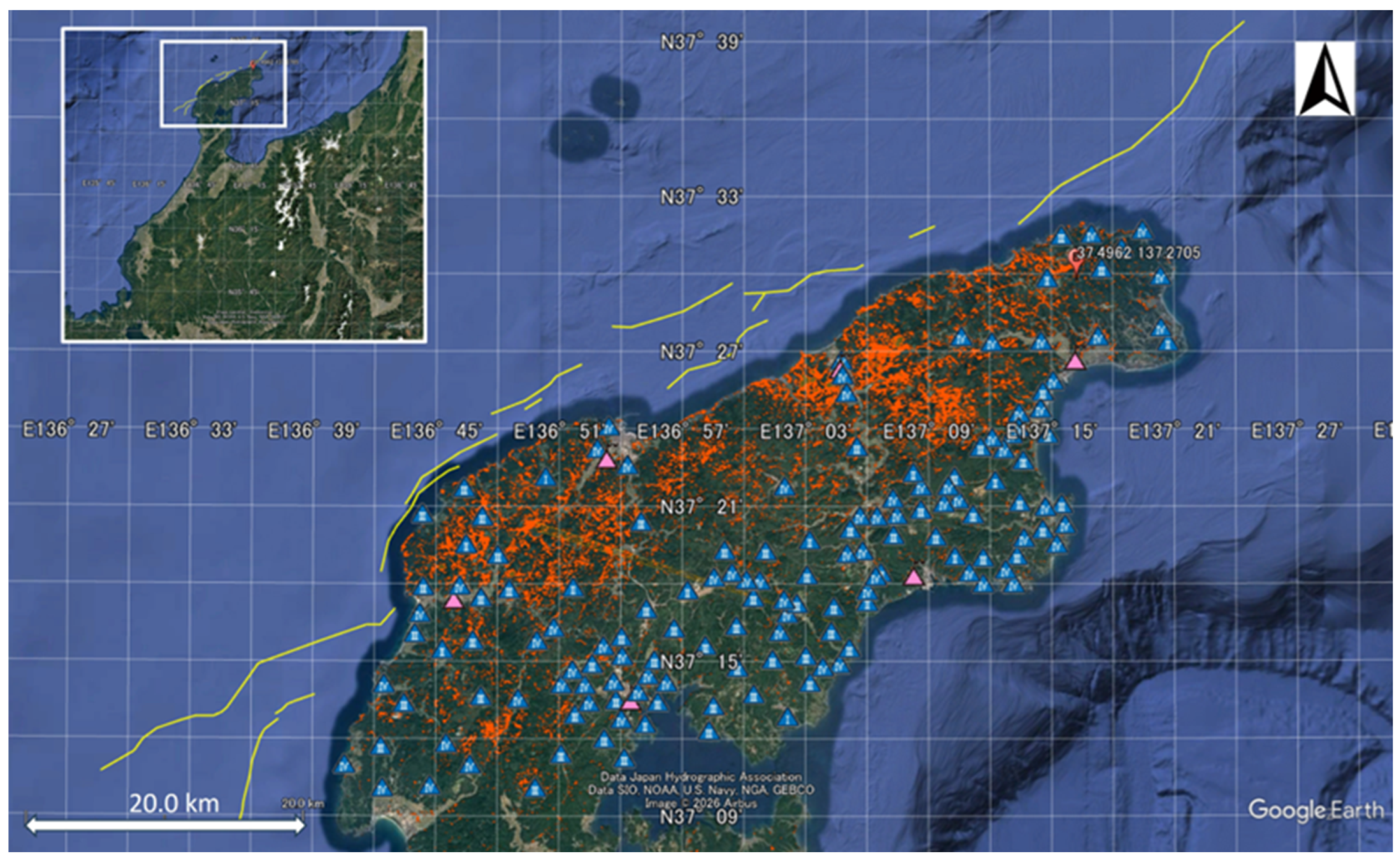
Figure 1 shows a satellite map of the study area—the northern part of the Noto Peninsula, Ishikawa Prefecture, Central Japan. In the figure, the epicenter is indicated by a red symbol [32], and the submarine fault segments that moved during the 2024 Noto Peninsula earthquake are shown by yellow lines [33]. The large crustal deformation was caused by sequential slips on northeast–southwest-striking, southeast-dipping submarine faults along the northern coast of the peninsula, following the continuing swarm since late 2020 [34,35]. Strong acceleration records exceeding 1 g were observed at several K-NET and KiK-net stations operated by the National Research Institute for Earth Science and Disaster Resilience (NIED) [36] and at one station operated by the Japan Meteorological Agency (JMA) [37]. Due to the intense shaking, numerous landslides and soil movements were observed in mountainous areas [38], as also plotted in the figure. Coseismic displacements were recorded at GEONET CORSs, shown by pink triangles, and at triangulation points, shown in blue (

Table A1. Locations and coseismic displacements of GNSS reference points obtained from GSI data [39] after the vertical datum conversion to JGD2011 [40,41].

No.	Station ID	Location in 2014			Coseismic Displacement (m)
		Long. (Deg.)	Lat. (Deg.)	Elev. (m)	Easting	Northing	Upward
1	EL05536677201	37.2264	136.9088	6.838	−0.890	0.222	0.016
2	EL05537716101	37.3070	137.1385	90.503	−0.642	0.207	0.061
3	EL05636075102	37.3824	136.8892	13.981	−1.191	−0.232	1.063
4	EL05637123103	37.4460	137.2701	12.468	−0.763	0.008	0.321
5	TR15537605201	37.2141	137.0355	113.390	−0.605	0.239	−0.075
6	TR15636064701	37.3688	136.8390	371.780	−1.164	−0.081	1.494
7	TR25536675301	37.2094	136.9199	43.240	−0.780	0.216	−0.011
8	TR25536760001	37.2574	136.7552	335.090	−0.708	−0.633	2.106
9	TR25536765801	37.2974	136.8614	254.910	−1.347	0.162	0.580
10	TR25536769101	37.3254	136.7745	341.590	−0.672	−0.174	2.735
11	TR25536775601	37.2956	136.9542	220.040	−1.177	−0.068	0.240
12	TR25537704801	37.2881	137.1001	135.580	−0.649	0.134	0.040
13	TR25537709401	37.3280	137.0534	254.450	−0.892	−0.092	0.347
14	TR25537718301	37.3176	137.1714	173.990	−0.606	0.253	0.127
15	TR25637013601	37.3663	137.2041	199.300	−0.670	0.254	0.068
16	TR25637014101	37.3715	137.1376	262.690	−0.754	−0.004	0.263
17	TR25637119901	37.4970	137.2466	296.950	−0.962	0.047	0.839
18	TR25637124701	37.4558	137.3450	28.090	−0.715	0.239	0.058
19	TR35536653601	37.1950	136.7054	210.890	−0.535	−0.328	0.640
20	TR35536656701	37.2228	136.7243	199.160	−1.313	−0.514	1.266
21	TR35536660601	37.1681	136.8308	275.380	−0.667	−0.002	0.033
22	TR35536662801	37.1899	136.8517	357.950	−0.699	0.215	0.033
23	TR35536665901	37.2154	136.8631	267.870	−0.931	0.118	0.131
24	TR35536667201	37.2271	136.7866	384.010	−1.076	−0.266	0.742
25	TR35536672201	37.1873	136.9031	59.400	−0.704	0.198	−0.018
26	TR35536673001	37.1998	136.8868	136.260	−0.739	0.255	0.015
27	TR35536674701	37.2051	136.9718	41.620	−0.691	0.207	−0.016
28	TR35536676101	37.2247	136.8963	77.120	−0.910	0.195	0.061
29	TR35536676401	37.2235	136.9301	36.150	−0.842	0.196	0.009
30	TR35536676801	37.2211	136.9753	69.880	−0.746	0.174	−0.004
31	TR35536679001	37.2481	136.8770	171.000	−1.104	0.139	0.221
32	TR35536679901	37.2458	136.9948	121.560	−0.882	0.110	−0.010
33	TR35536752801	37.2678	136.7329	111.770	−1.775	−0.762	2.743
34	TR35536755901	37.2980	136.7397	163.650	−1.374	−0.494	3.638
35	TR35536761201	37.2632	136.7800	336.180	−1.175	−0.046	1.079
36	TR35536764201	37.2909	136.7866	66.960	−0.906	−0.080	1.950
37	TR35536765401	37.2963	136.8095	239.950	−1.209	−0.153	0.767
38	TR35536768401	37.3185	136.8003	223.230	−1.374	−0.187	1.332
39	TR35536770401	37.2506	136.9274	109.750	−1.000	0.129	0.114
40	TR35536771201	37.2655	136.9008	158.840	−1.139	0.115	0.211
41	TR35536771701	37.2599	136.9688	145.310	−0.952	0.063	0.100
42	TR35536772501	37.2711	136.9434	168.810	−1.069	0.041	0.152
43	TR35536772901	37.2727	136.9939	190.130	−0.934	0.030	0.133
44	TR35536774301	37.2835	136.9208	200.020	−1.203	0.045	0.116
45	TR35536778801	37.3213	136.9843	261.380	−1.124	−0.151	0.435
46	TR35537607001	37.2286	137.0080	91.200	−0.709	0.169	−0.008
47	TR35537608401	37.2361	137.0536	80.880	−0.640	0.185	−0.018
48	TR35537700101	37.2510	137.0233	181.290	−0.755	0.118	0.042
49	TR35537700401	37.2533	137.0504	122.930	−0.688	0.136	0.031
50	TR35537700601	37.2583	137.0856	64.450	−0.610	0.174	0.012
51	TR35537702501	37.2690	137.0709	128.510	−0.668	0.125	0.060
52	TR35537704001	37.2910	137.0077	189.330	−0.965	−0.009	0.195
53	TR35537704301	37.2871	137.0430	167.240	−0.800	0.036	0.151
54	TR35537704501	37.2849	137.0730	148.020	−0.702	0.086	0.100
55	TR35537706401	37.3054	137.0512	203.620	−0.825	−0.015	0.234
56	TR35537706801	37.3070	137.1112	169.120	−0.701	0.128	0.070
57	TR35537708101	37.3211	137.0176	254.640	−1.042	−0.077	0.350
58	TR35537709901	37.3313	137.1215	199.700	−0.800	0.113	0.142
59	TR35537718501	37.3168	137.1943	157.710	−0.564	0.238	0.001
60	TR35537718701	37.3179	137.2218	112.060	−0.509	0.225	−0.003
61	TR35537719201	37.3303	137.1558	184.850	−0.704	0.199	0.056
62	TR35636051901	37.3449	136.7389	107.690	−1.465	0.185	4.107
63	TR35636061301	37.3431	136.7876	293.270	−1.138	0.515	2.132
64	TR35636063101	37.3616	136.7728	313.670	−1.188	0.587	2.291
65	TR35636070301	37.3399	136.9165	280.250	−1.483	−0.008	0.492
66	TR35636078201	37.4047	136.9018	4.580	−1.530	−0.284	1.609
67	TR35637000601	37.3352	137.0863	199.750	−0.892	−0.018	0.255
68	TR35637006701	37.3883	137.0918	184.140	−1.357	−0.252	0.585
69	TR35637010901	37.3348	137.2427	56.530	−0.507	0.207	0.025
70	TR35637011101	37.3476	137.1437	217.340	−0.825	0.148	0.115
71	TR35637011401	37.3446	137.1861	152.920	−0.662	0.226	0.050
72	TR35637012701	37.3524	137.2240	99.820	−0.581	0.226	0.052
73	TR35637014301	37.3687	137.1711	240.030	−0.831	0.197	0.117
74	TR35637015801	37.3795	137.2269	133.150	−0.664	0.215	0.103
75	TR35637016501	37.3880	137.1922	202.990	−0.840	0.238	0.137
76	TR35637017901	37.3963	137.2469	28.340	−0.668	0.161	0.131
77	TR35637022001	37.3511	137.2581	35.060	−0.516	0.179	0.036
78	TR35637110901	37.4238	137.2430	48.360	−0.798	0.171	0.212
79	TR35637220301	37.5033	137.2911	213.820	−1.100	0.117	0.862
80	TR35637222001	37.5244	137.2584	155.940	−1.550	0.610	1.510
81	TR45536650601	37.1680	136.7067	5.360	−0.232	−0.385	0.411
82	TR45536650901	37.1695	136.7453	36.890	−0.324	−0.408	0.399
83	TR45536651401	37.1831	136.6760	4.970	−0.235	−0.227	0.197
84	TR45536658601	37.2350	136.7080	47.690	−0.881	−0.693	0.939
85	TR45536661201	37.1830	136.7778	67.060	−0.644	−0.268	0.187
86	TR45536663001	37.1969	136.7585	233.430	−0.611	−0.249	0.742
87	TR45536666901	37.2232	136.8743	166.840	−0.937	0.147	0.107
88	TR45536667501	37.2257	136.8168	240.340	−1.045	−0.053	0.423
89	TR45536668801	37.2350	136.8520	227.710	−1.056	0.116	0.193
90	TR45536668901	37.2346	136.8710	181.080	−1.018	0.136	0.179
91	TR45536669801	37.2440	136.8610	170.200	−1.183	0.340	0.043
92	TR45536675201	37.2125	136.9006	57.350	−0.833	0.202	0.010
93	TR45536677301	37.2301	136.9142	61.750	−0.906	0.204	0.038
94	TR45536678102	37.2366	136.8944	22.220	−0.988	0.175	0.113
95	TR45536678301	37.2409	136.9222	78.560	−0.954	0.164	0.081
96	TR45536678401	37.2361	136.9372	56.610	−0.900	0.203	0.002
97	TR45536753801	37.2808	136.7370	74.070	−2.223	−0.268	3.251
98	TR45536761601	37.2631	136.8320	146.450	−1.198	0.043	0.646
99	TR45536762701	37.2714	136.8458	80.380	−1.314	0.094	0.516
100	TR45536765101	37.2985	136.7692	156.050	−0.340	−0.280	2.022
101	TR45536770201	37.2532	136.9013	114.810	−1.074	0.140	0.177
102	TR45536771001	37.2598	136.8861	157.360	−1.160	0.146	0.192
103	TR45536776801	37.3040	136.9757	276.410	−1.129	−0.057	0.272
104	TR45536776901	37.3070	136.9903	201.860	−1.084	−0.054	0.291
105	TR45537609501	37.2461	137.0641	82.220	−0.629	0.177	0.002
106	TR45537609601	37.2482	137.0775	71.870	−0.644	0.154	−0.007
107	TR45537702201	37.2689	137.0289	141.070	−0.800	0.075	0.101
108	TR45537703201	37.2805	137.0353	148.130	−0.805	0.050	0.131
109	TR45537704201	37.2895	137.0325	128.220	−0.846	0.020	0.173
110	TR45537705801	37.2954	137.1002	150.250	−0.672	0.121	0.050
111	TR45537706001	37.3024	137.0021	206.900	−1.027	−0.039	0.259
112	TR45537706101	37.3019	137.0128	204.240	−0.982	−0.033	0.248
113	TR45537706802	37.3046	137.1070	163.340	−0.697	0.118	0.070
114	TR45537708601	37.3194	137.0838	174.610	−0.808	0.014	0.195
115	TR45537708701	37.3211	137.0964	172.610	−0.793	0.047	0.175
116	TR45537715701	37.3000	137.2191	76.250	−0.673	0.379	0.023
117	TR45537716401	37.3071	137.1829	128.180	−0.565	0.247	0.000
118	TR45537716501	37.3001	137.1943	64.280	−0.532	0.261	0.004
119	TR45537717701	37.3090	137.2126	100.540	−0.508	0.232	−0.013
120	TR45537719801	37.3294	137.2274	84.290	−0.522	0.221	0.006
121	TR45537729001	37.3254	137.2541	9.450	−0.476	0.199	0.000
122	TR45636075201	37.3764	136.9054	14.360	−1.600	0.040	0.713
123	TR45636076001	37.3869	136.8809	128.750	−1.220	−0.453	1.213
124	TR45636078101	37.4014	136.8902	7.230	−1.593	0.019	1.523
125	TR45637001701	37.3436	137.0942	198.260	−0.931	−0.012	0.274
126	TR45637001801	37.3433	137.1081	190.860	−0.903	0.042	0.224
127	TR45637001901	37.3443	137.1242	209.190	−0.870	0.098	0.183
128	TR45637002901	37.3549	137.1211	151.610	−0.943	0.070	0.234
129	TR45637003201	37.3626	137.0331	199.720	−1.113	−0.189	0.530
130	TR45637011901	37.3494	137.2449	23.650	−0.534	0.196	0.039
131	TR45637012201	37.3519	137.1623	201.800	−0.779	0.183	0.097
132	TR45637012301	37.3544	137.1741	191.990	−0.748	0.207	0.088
133	TR45637013101	37.3626	137.1438	244.780	−0.901	0.120	0.163
134	TR45637013301	37.3628	137.1659	217.470	−0.821	0.186	0.116
135	TR45637016601	37.3866	137.2111	131.800	−0.750	0.242	0.115
136	TR45637017601	37.3940	137.2016	166.870	−0.742	0.132	0.207
137	TR45637017701	37.3963	137.2178	15.160	−0.774	0.234	0.138
138	TR45637018701	37.4007	137.2232	55.880	−0.772	0.223	0.149
139	TR45637019701	37.4100	137.2236	56.680	−0.818	0.234	0.182
140	TR45637019901	37.4128	137.2411	44.430	−0.755	0.175	0.169
141	TR45637020001	37.3381	137.2609	29.580	−0.669	0.327	−0.127
142	TR45637100601	37.4231	137.0833	9.980	−1.531	−0.476	1.032
143	TR45637102601	37.4344	137.0802	5.990	−1.548	−0.269	1.470
144	TR45637103601	37.4441	137.0792	11.560	−1.825	−0.332	1.715
145	TR45637114601	37.4558	137.2015	65.450	−1.206	0.495	0.734
146	TR45637114901	37.4564	137.2416	18.410	−0.929	−0.004	0.528
147	TR45637115401	37.4593	137.1767	173.380	−0.964	−0.948	0.671
148	TR45637121001	37.4308	137.2514	4.720	−0.632	−0.078	0.143
149	TR45637125301	37.4594	137.2880	6.150	−0.670	0.062	0.341
150	TR45637125701	37.4651	137.3392	4.510	−0.796	0.195	0.047
151	TR45637129701	37.4984	137.3390	47.380	−0.916	0.124	0.415
152	TR45637221401	37.5163	137.3074	121.550	−1.050	0.221	0.993
153	TR45637223201	37.5255	137.2829	21.950	−1.672	0.917	1.486
154	TR45637223501	37.5281	137.3245	43.600	−0.952	0.025	1.093

), with their ranks indicated by Roman numerals. Of the six GEONET stations, real-time coordinates and elevations were released for four stations (Wajima, Suzu, Noto, and Anamizu) soon after the earthquake, showing that huge crustal movements had occurred on the peninsula. In contrast, two stations (Wajima-2a in Machino and Wajima-3 in Monzen) were deployed after the event.

GNSS surveys were conducted by the GSI at 150 triangulation points before the earthquake (April 2014) and after the earthquake (from April to December 2024). The post-event data were available online [39], and the pre-event data were provided by the GSI in June 2025. Note that the Japanese geodetic datum was updated from the “Japanese Geodetic Datum 2011 (JGD2011)” to the latest “Japanese Geodetic Datum 2024 (JGD2024)”, effective 1 April 2025 [40]. This update aims to eliminate differences among survey results caused by the long-term accumulation of crustal deformation and to enable the more rapid determination of the orthometric height by GNSS observations using the newly implemented “Geoid 2024: Japan and its surroundings”. Therefore, to obtain the change in orthometric height at the 150 triangulation points, the post-event data were adjusted using the API [41]. In the study area, Geoid 2024 is 17–22 cm lower than Geoid 2011; therefore, these values should be added to convert JGD2024 data to JGD2011 data.

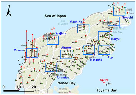
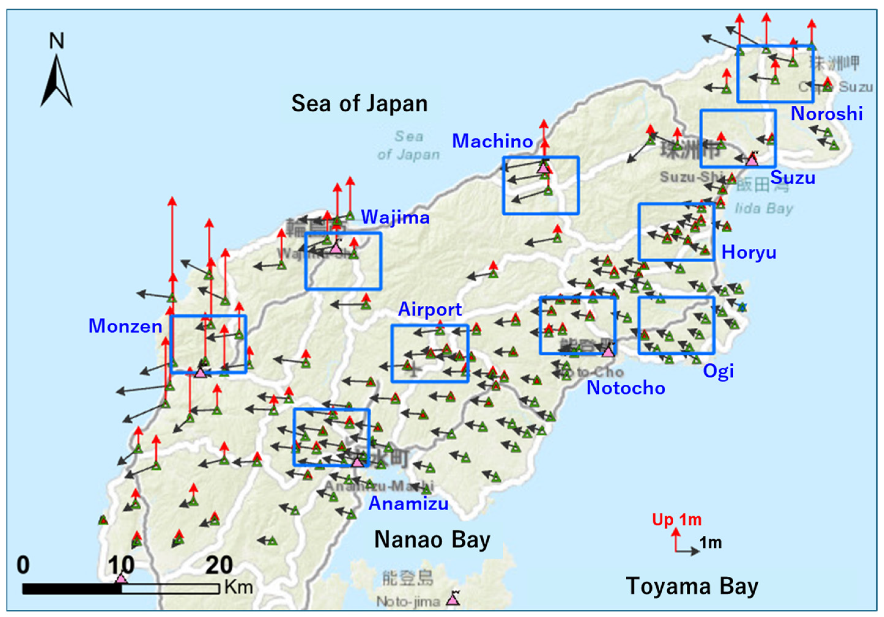
Figure 2 and Table A1 show the locations and the horizontal and vertical coseismic displacements at the 4 GEONET CORSs and 150 triangulation points in the study area. Vertical displacements were upward along the northern coast and almost zero along the southern coast. The maximum uplift (4.11 m) was recorded at the Isuzu point (TR35636051901), followed by 3.64 m at the Miyamaruyama point (TR35536755901), both in the Monzen district of Wajima City. Westward displacements dominated the horizontal field, with a maximum value of 2.22 m at the Kuroshima point (TR45536753801) in Monzen. Although the density of the triangulation points is relatively high in the southern part of the peninsula, sparse or blank areas exist along the northern coastline. Thus, spatial interpolation of the observed displacements is not straightforward.

The GNSS observation data (Figure 2 and Table A1) may include post-seismic displacements that occurred between the main shock on 1 January 2024 and the GNSS survey dates (April–December 2024). At the Wajima GEONET station, cumulative post-seismic displacements during the year following the main shock were approximately 0.7 cm westward, 2.8 cm northward, and 11.1 cm downward [42]. These values are substantially smaller than the meter-scale displacements caused by the main shock of the 2024 Noto Peninsula earthquake. Therefore, the contribution of post-seismic deformation to the GNSS-based displacement measurements is considered minor.

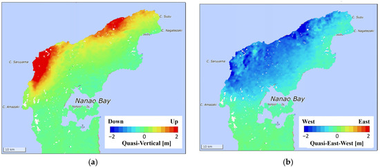
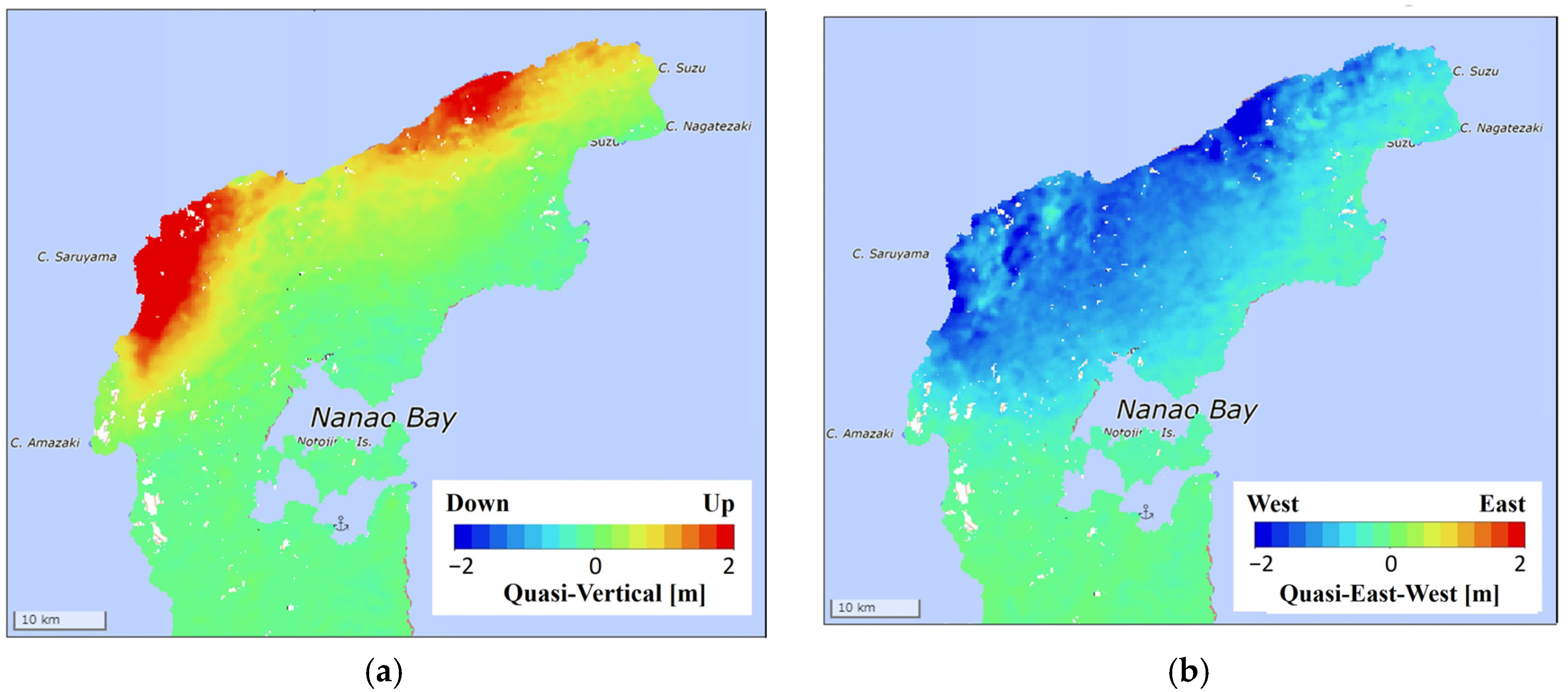
Coseismic displacements can also be estimated from satellite SAR data. Figure 3 shows the 2.5-dimensional results from pixel-offset (tracking) analyses of multi-path ALOS-2 intensity data, produced by the GSI [2,43]. Although the 2.5D analysis provides only quasi-UD and quasi-EW displacements, it captures the overall trend of the horizontal displacement field because the NS displacement is relatively small, as shown in Figure 2. The maximum quasi-UD displacement was about 4 m in the Monzen area, consistent with the GNSS observations. Uplift of about 2 m was estimated along the northeastern coastline of Suzu City, where triangulation points are sparse. The UD displacement decreases from the northern coastline toward the southern coastline. In contrast, the quasi-EW displacement is distributed more uniformly across the peninsula, from about 2 m along the northern coast to about 1 m along the southern coast. To perform ICP analysis of airborne LiDAR data, square regions excluding the sea must be selected. Therefore, ten square regions measuring 6.0 km (EW) × 4.5 km (NS) were selected, as shown in Figure 2, taking into account the distribution of GNSS survey points and coseismic displacements. Out of 154 reference points, 59 of them are included inside the ten study areas.

2.2. Airborne LiDAR Data Used in the Study

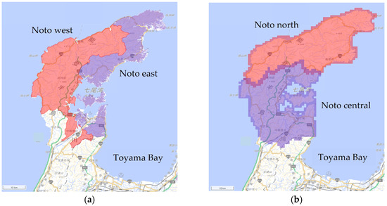
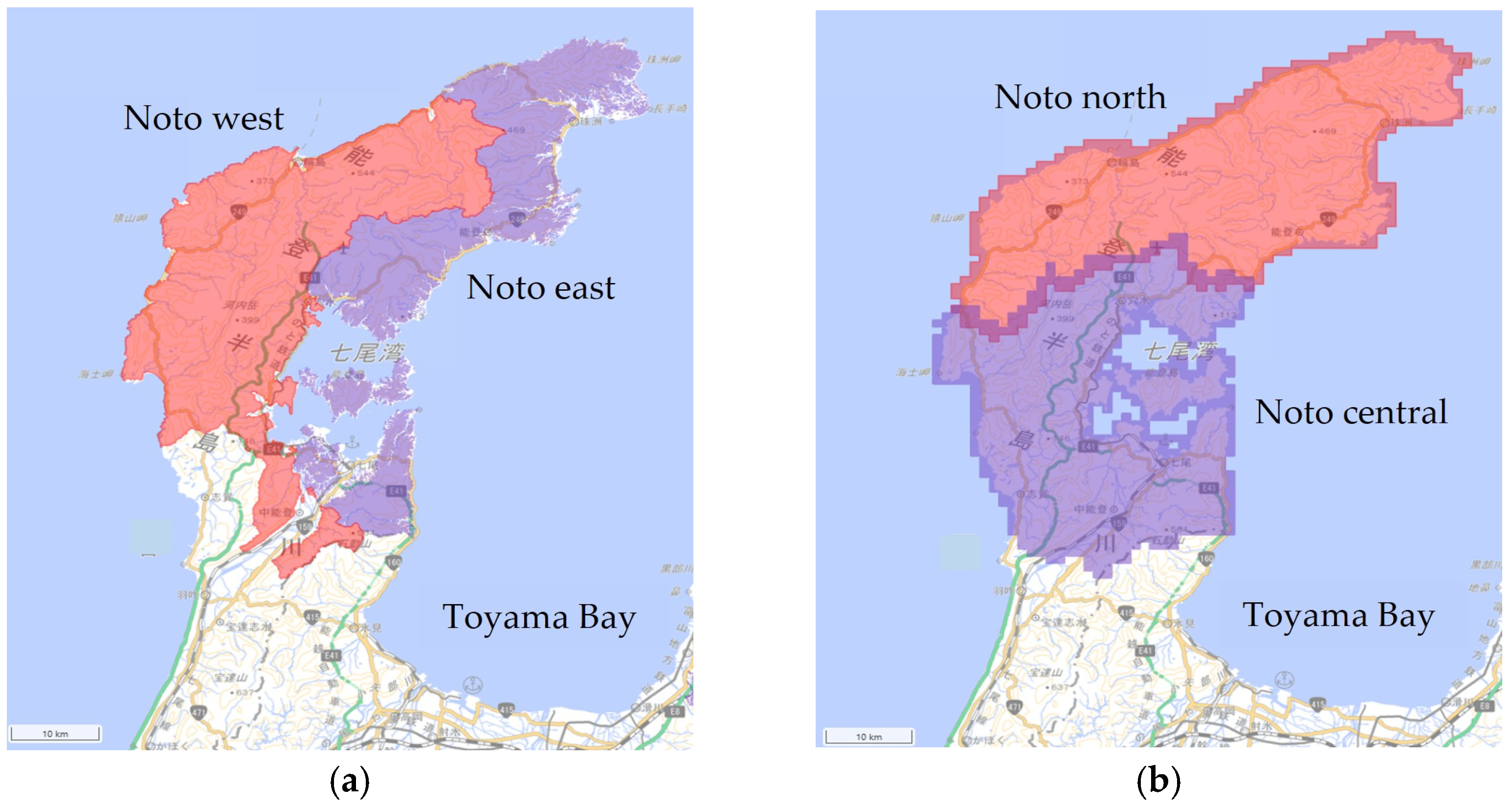
The areas covered by the pre-event and post-event airborne LiDAR data used in this study are shown in Figure 4 and

Table 1. Airborne LiDAR datasets used in this study [24,25].

Dataset	Ishikawa Prefectural Gov. (Pre-EQ)		Forestry Agency (Post-EQ)
Project	FY2020 Forestry DX (Noto west)	FY2022 Forestry DX (Noto east)	Airborne LiDAR (Noto north)	Airborne LiDAR (Noto central)
Observation Dates	02/07/2020–31/03/2021	02/08/2022–09/10/2022	11/03/2024–28/04/2024	11/03/2024–04/05/2024
Point Density (1/m2)	4.0	4.0	4.0	4.0
Data Form	Point cloud	Point cloud	0.5 m DEM	0.5 m DEM

. The pre-event data were acquired by the Department of Agriculture, Forestry, and Fisheries of the Ishikawa Prefectural Government as part of a digital transformation project for forestry information in fiscal years 2020 and 2022. The dataset covers the northern part of the peninsula and consists of high-density original point-cloud data (4.0 points/m²). Since February 2024, the dataset has been available as open data for non-commercial use to support recovery and reconstruction activities [24].

The post-event airborne LiDAR data were acquired through a joint survey project of the Geospatial Information Authority of Japan (GSI) and the Forestry Agency of Japan (FA). The dataset covers the entire peninsula at a density of 4.0 points/m². The original point-cloud data were processed by the FA into digital elevation (terrain) models (DEMs) with a 0.5 m grid by removing trees and buildings, and the DEMs were released as open data in April 2025 [25]. By comparing these pre- and post-event airborne LiDAR datasets, we carried out a 3D topographic differencing (3DTD) analysis based on the Iterative Closest Point (ICP) algorithm [26,27,28].

The post-event LiDAR surveys were conducted prior to the heavy rainfall event of September 2024 [44] that triggered additional landsliding in the study area. Consequently, these later slope failures are not included in the analyzed LiDAR datasets. The post-event LiDAR data may also include a minor component of post-seismic crustal deformation. However, as discussed above for the GNSS observations, its contribution to the LiDAR-derived displacement field is considered small relative to the coseismic deformation associated with the main shock. Accordingly, the displacement field derived in this study is interpreted as being predominantly coseismic, although a minor post-seismic contribution cannot be completely excluded.

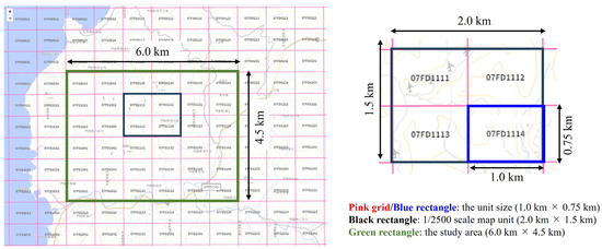
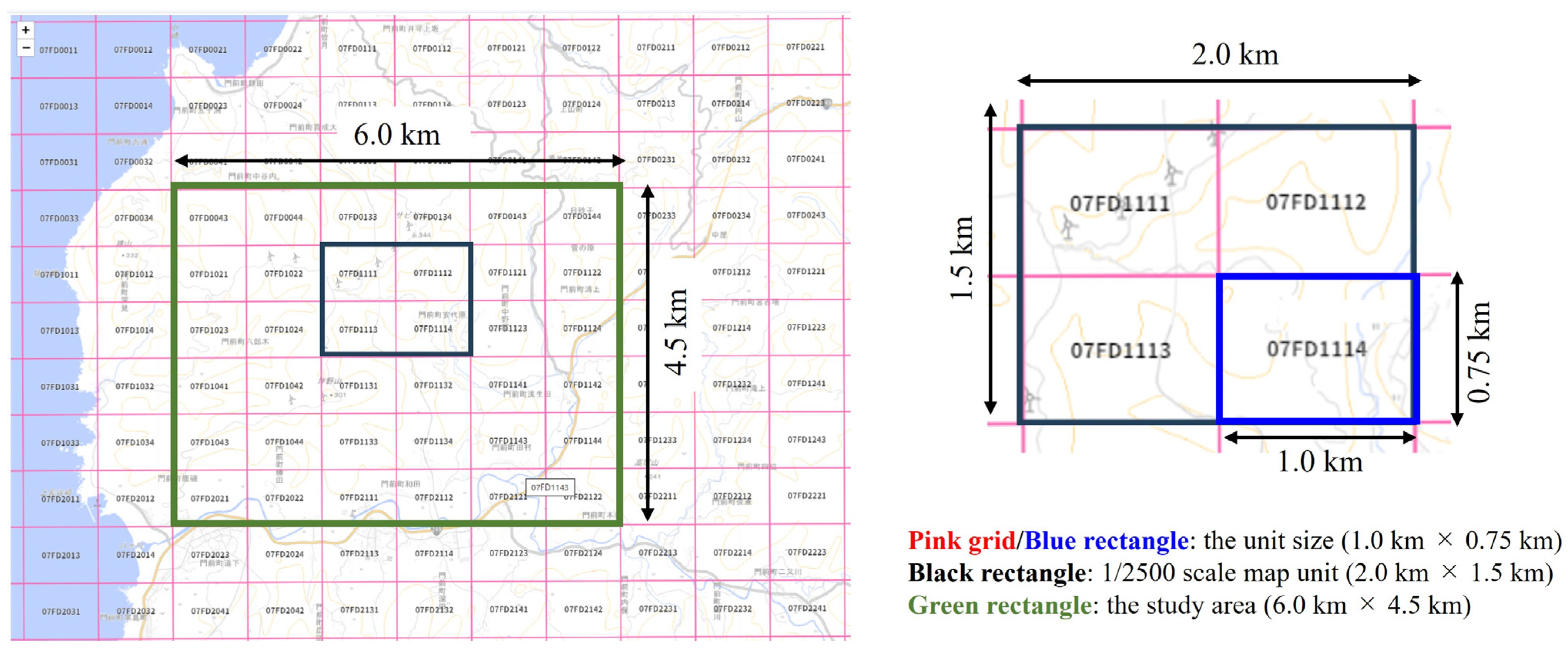
To examine the validity of the ICP algorithm for extracting coseismic displacements associated with the 2024 Noto Peninsula earthquake, the Monzen district in the western part of Wajima City was selected because the largest crustal movement was observed there. Figure 5 shows the projected map of the pre-event LiDAR data for Monzen. Considering the computational cost of the ICP analysis, a sample area of 6.0 km (EW) × 4.5 km (NS) was selected; this area is composed of 6 × 6 (=36) standard airborne LiDAR data units (1.0 km × 0.75 km) in Japan. Using the ENVI LiDAR software (version 6.1) [45], a DEM with 0.5 m spacing in GeoTIFF format was created from the original point-cloud (LAS) data.

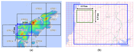
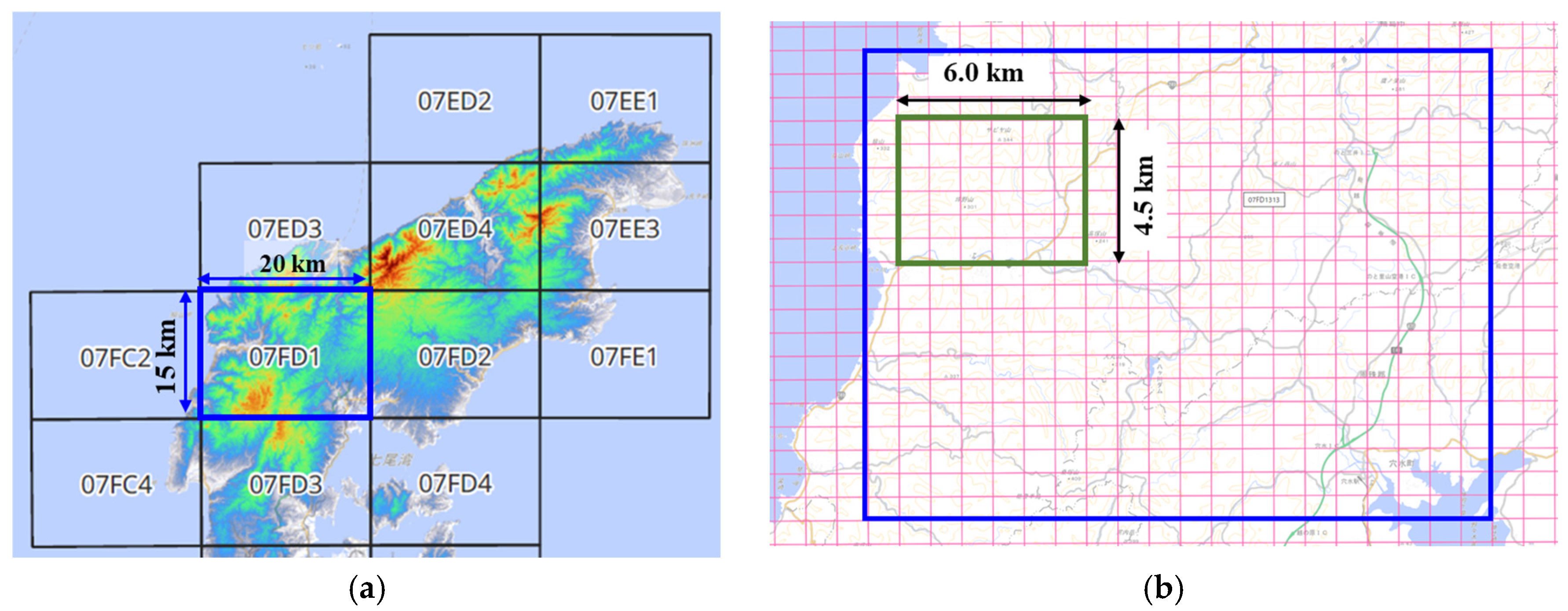
The post-event LiDAR data were released in much larger units, as shown in Figure 6. The processed DEM data with 0.5 m spacing cover a rectangle measuring 20 km (EW) × 15 km (NS). An area of the same size and location as the pre-event data in Monzen was extracted in GeoTIFF format using the ENVI software (version 6.1) [45], as also shown in the figure. Both the pre-event and post-event DEM data were then converted to point-cloud data (LAS format) using the CloudCompare freeware (version 2.1.4) [46] to conduct the ICP analysis.

2.3. The Iterative Closest Point (ICP) Method

In our previous study on extracting crustal movements from airborne LiDAR data for the 2016 Kumamoto earthquake [47], the pixel-offset method was used to obtain horizontal movements, and vertical differencing was then conducted to derive vertical displacements in Mashiki Town, Kumamoto Prefecture, Japan. In recent years, a 3D topographic differencing analysis tool based on the Iterative Closest Point (ICP) algorithm has become available online [48], and Python (version 3) and MATLAB programs have also been released [49]. We tested the Python program using digital surface model (DSM) data for Mashiki Town and obtained results almost identical to those from our pixel-offset analysis. Therefore, in this study, we use the ICP method available through OpenTopography [49,50] to extract crustal movements associated with the 2024 Noto Peninsula earthquake from airborne LiDAR data.

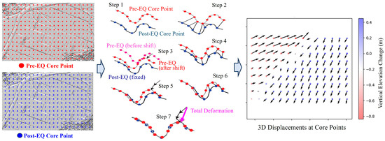
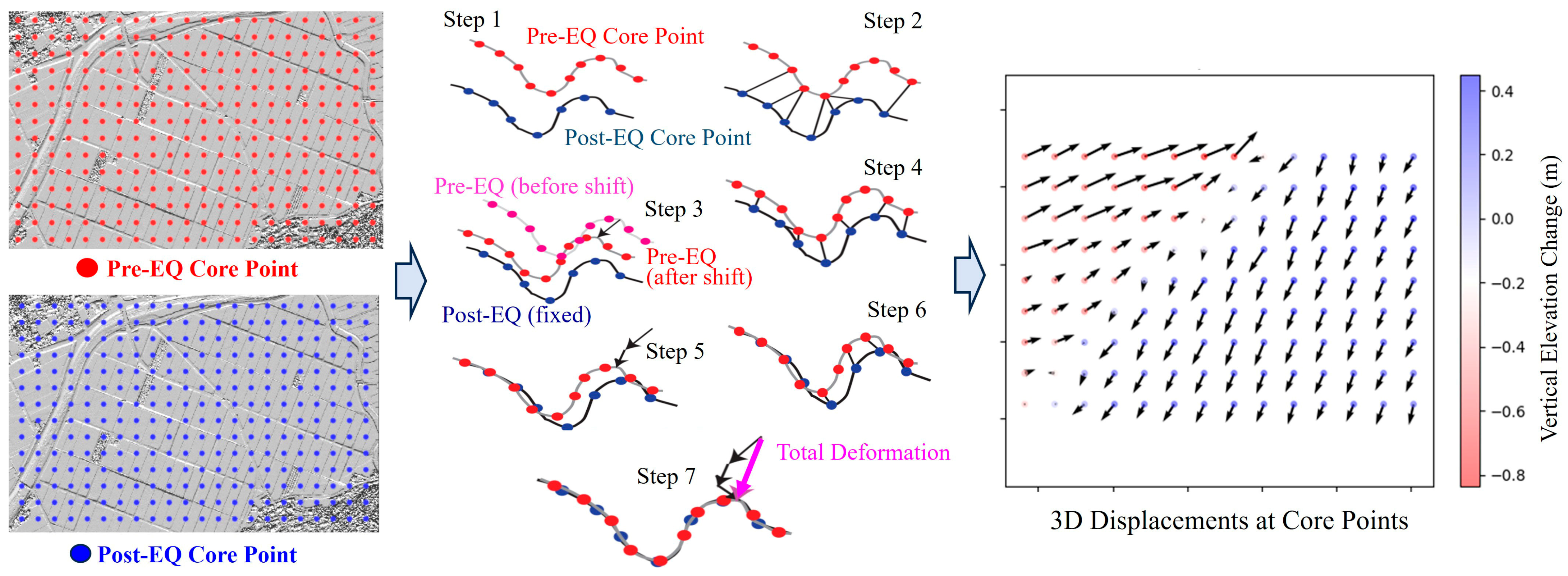
Figure 7 shows the schematic flow of the ICP method available on the OpenTopography (OT) website. First, core points representing the centers of square tiles (windows) are assigned for the pre- and post-event point clouds. Then, a 3D rigid-body transformation with translation and rotation is iteratively searched to bring the two sets of core points as close as possible in 3D space. For a pre-event (comparison) window width x, the post-event (reference) window width is set to x + buffer, allowing for a possible offset corresponding to the maximum correlation outside the common tiles. This method has been successfully applied to the 2008 Iwate–Miyagi (Mw 6.9) earthquake [27], the 2011 Fukushima–Hamadori (Mw 7.1) earthquake [27], and the 2016 Kumamoto earthquake [28].

2.4. Moving Average of the ICP Results

In the above-mentioned ICP method, the most important parameter is the common tile (window) size for the pre- and post-event LiDAR point-cloud data. Scott et al. [50] suggested that the appropriate window size is a function of the LiDAR point-cloud density: 45 m for all original points and 32 m for ground points. We tested several window sizes for the Noto LiDAR datasets. In the northern part of the peninsula, coseismic displacements were large, and numerous landslides and soil movements were observed (Figure 1). If a window includes part of a landslide-affected zone, the ICP method may still find a high-correlation 3D displacement, but this displacement may not represent the regional crustal movement. Therefore, a moving-average scheme is introduced to reduce the effects of ground-surface irregularity and obtain smooth coseismic displacements. Another reason for introducing the moving-average scheme is to reduce the effect of the grid layout of the window tiles. A large window is suitable for representing crustal movement over a wide area, but it increases the influence of the grid layout. Thus, the moving-average scheme is introduced to represent wide-area crustal movement while minimizing grid layout effects.

For the purpose of this study, the displacement field, d^T = [d_x, d_y, d_z], is separated into a long-wavelength component and a short-wavelength residual component using a spatial filtering technique. The former is interpreted primarily as crustal deformation (d_crustal), whereas the latter is expected to emphasize localized ground failures (d_local) such as landslides.

$$\mathbf{d}={\mathbf{d}}_{crustal}+{\mathbf{d}}_{local}$$

(1)

The wavelength of the crustal deformation varies smoothly over distances of several kilometers to tens of kilometers, as shown in Figure 3. In contrast, local ground movement has a much smaller scale, namely several tens to hundreds of meters, based on the size of the landslides in the Noto Peninsula earthquake [38].

In the present study, the simple moving-average filter was selected because of its simplicity, transparency, and computational efficiency in processing large-area LiDAR datasets and because the primary objective was to extract broad spatial trends in coseismic deformation rather than to optimize the filtering methodology. A systematic comparison of alternative filtering methods is beyond the scope of the present study and is identified as a topic for future work.

A two-dimensional (2D) simple moving average (SMA) filter for a window centered at (n, m) with size (2k + 1)(2l + 1) is written as

$${\mathbf{d}}_{crustal}\left(n, m\right)={\displaystyle \frac{1}{\left(2k+1\right)\left(2l+1\right)}}{\displaystyle \sum _{i=n-k}^{n+k}}{\displaystyle \sum _{j=m-l}^{m+l}}\mathbf{d}(i, j)$$

(2)

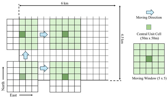
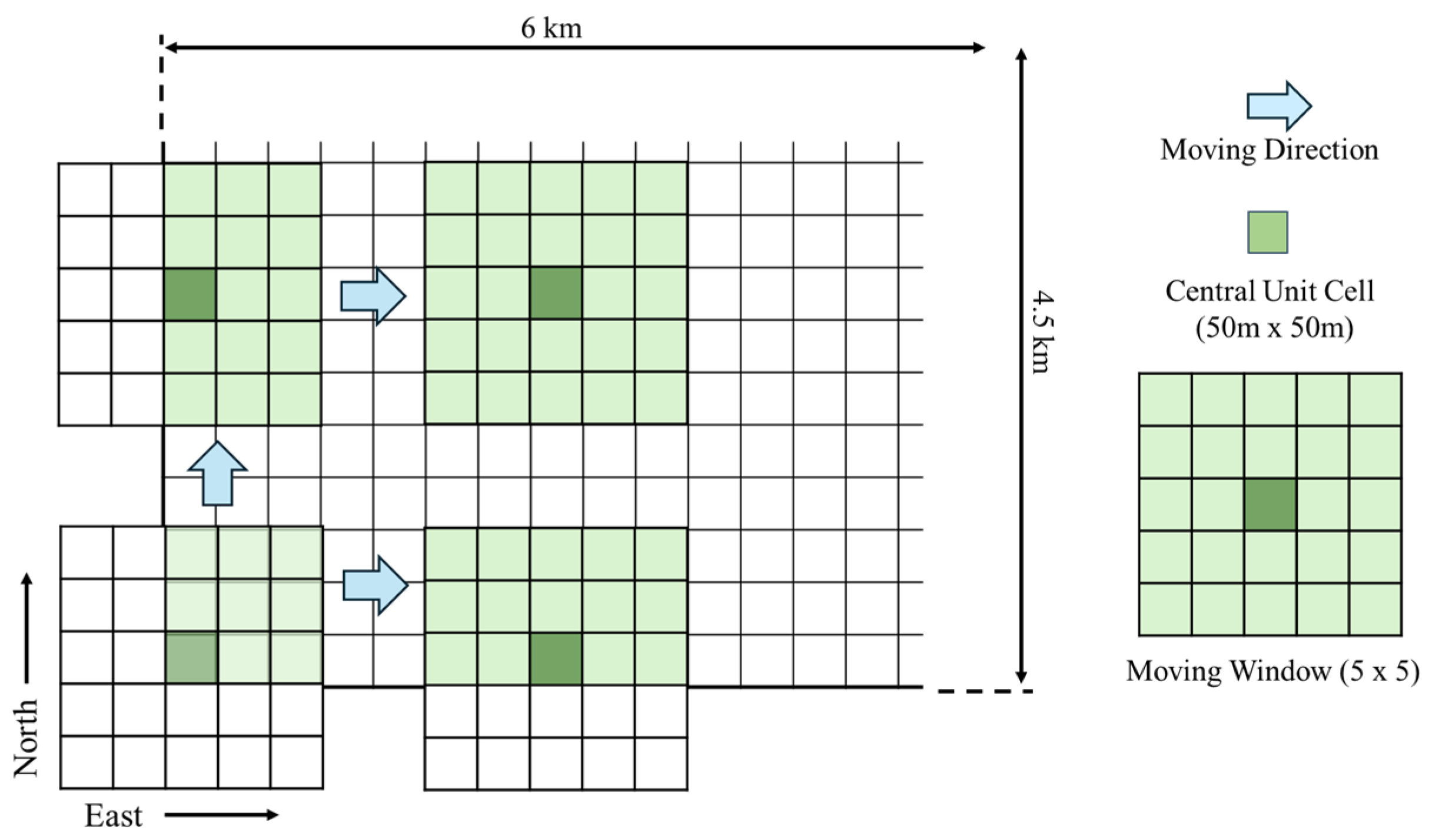
where d_crustal (n, m) is the averaged (filtered) value at row n and column m, d(i, j) is the original input data value at row i and column j, and k and l are the radii of the moving-average window in the y and x directions, respectively. The total number of tiles in the neighborhood (window size) is (2k + 1)(2l + 1). A schematic of the 2D moving average for the case k = l = 2 is shown in Figure 8. If the moving window extends beyond the pre-event data range and the central unit tile of the window is still within the post-event data range, the averaging operation is applied using only the valid tiles within the data range.

The original input tile size was selected as 50 m × 50 m after several trials in this study. The local ground movement at row n and column m is then obtained as

$${\mathbf{d}}_{local}\left(n, m\right)=\mathbf{d}\left(n, m\right)-{\mathbf{d}}_{crustal}\left(n, m\right)$$

(3)

where d_local(n, m) is the residual coseismic displacement after the removal of the crustal movement (trend) component.

3. Results

3.1. The 3D Crustal Movement in Monzen District, Wajima City

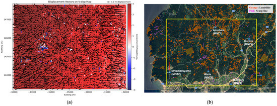
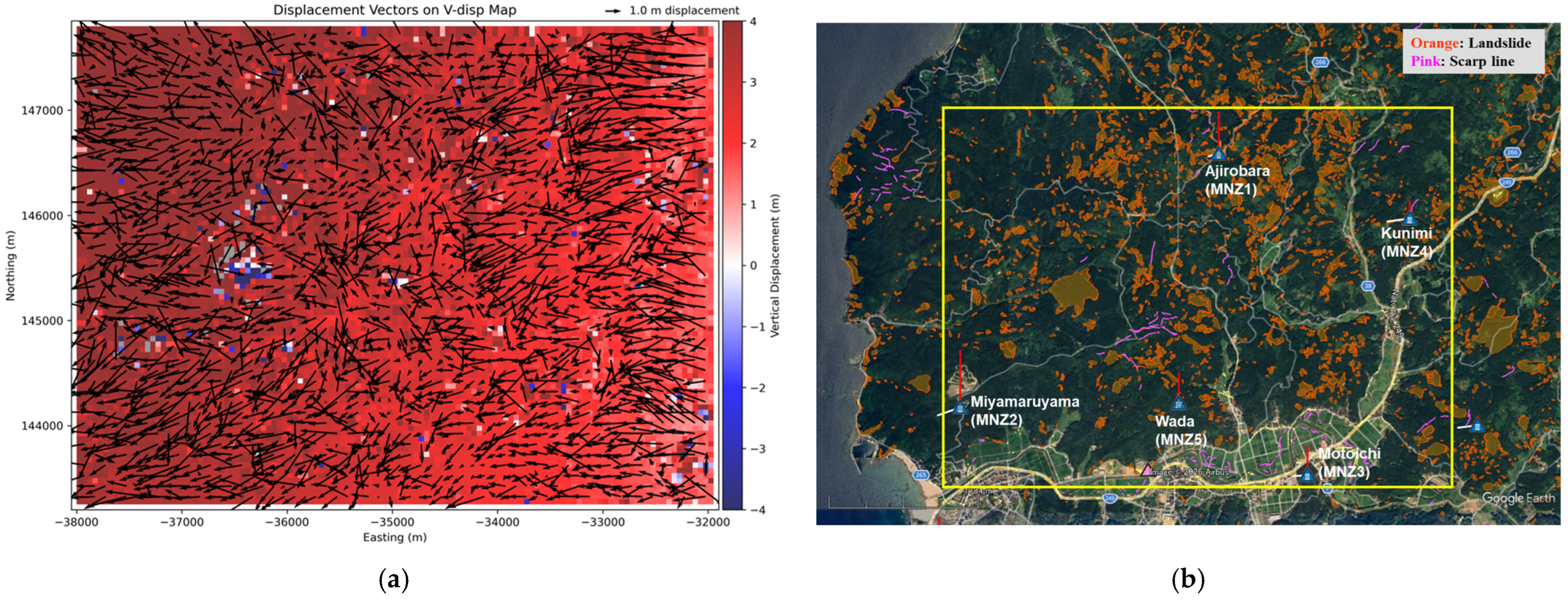
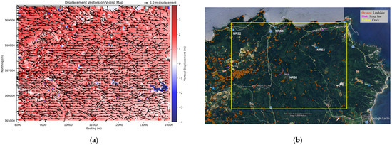
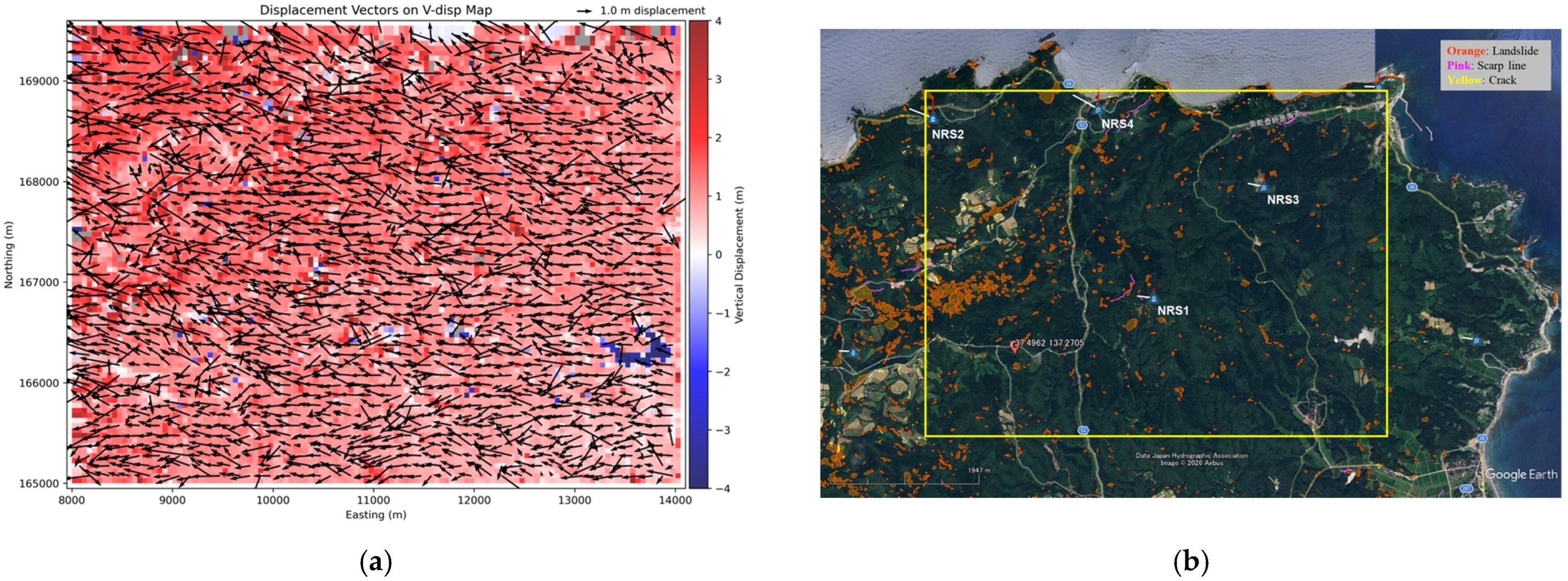
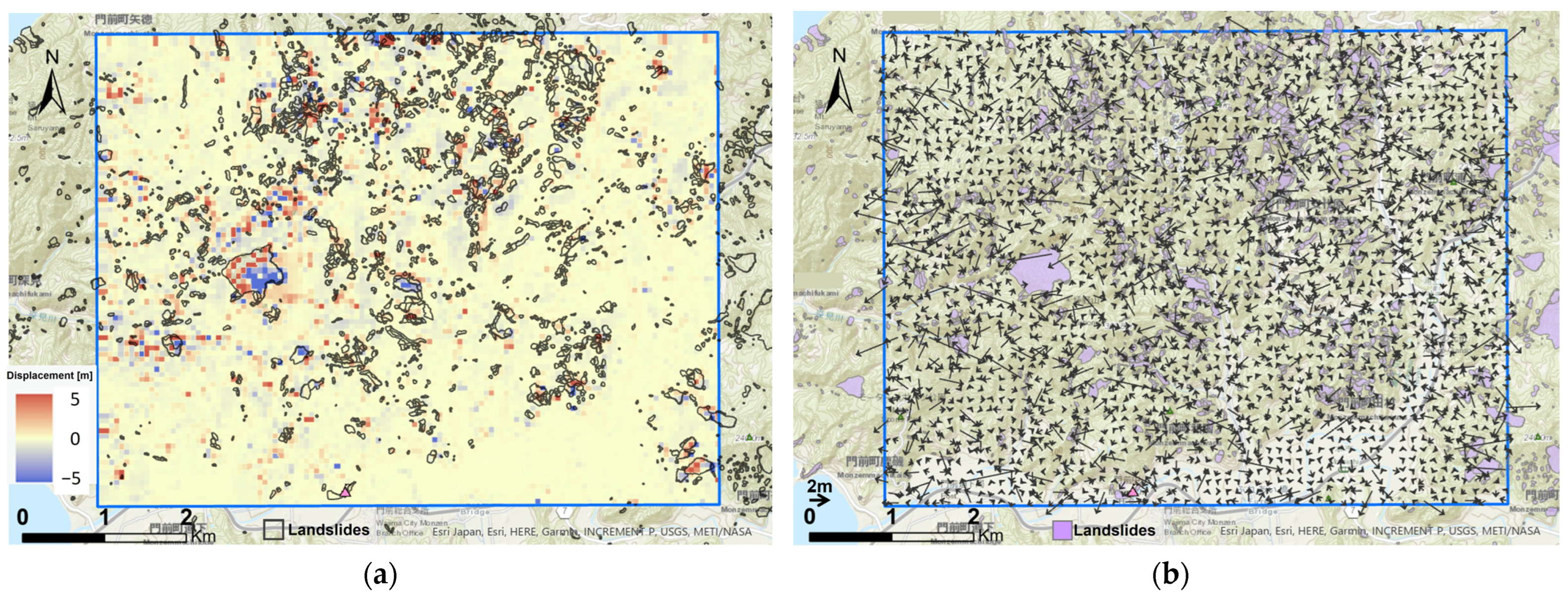
For the prepared pre- and post-event DEM data for the Monzen district in the western part of Wajima City, the ICP analysis was carried out using the Python code [49]. For the selected study area of 6.0 km (EW) × 4.5 km (NS), the analysis result for 50 m windows (tiles) is shown in Figure 9a, where horizontal coseismic displacements are plotted as arrows at 100 m intervals and vertical displacements are shown by colors for 50 m square tiles. To examine the causes of variations in the coseismic displacements, the landslide polygons and surface scarp lines [38], both visually extracted from the same LiDAR datasets, are shown in Figure 9b, together with five triangulation points in this study area. Considerable parts of the ground surface, especially forested areas, were clearly affected by slope failures (orange color). Disturbances in the coseismic displacements are co-located with the slope failures; for example, at the largest landslide location, the vertical displacement shows blue (negative) or gray (no data) colors. The orientation of the horizontal displacement also becomes unstable at these soil failure locations.

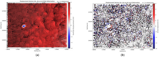
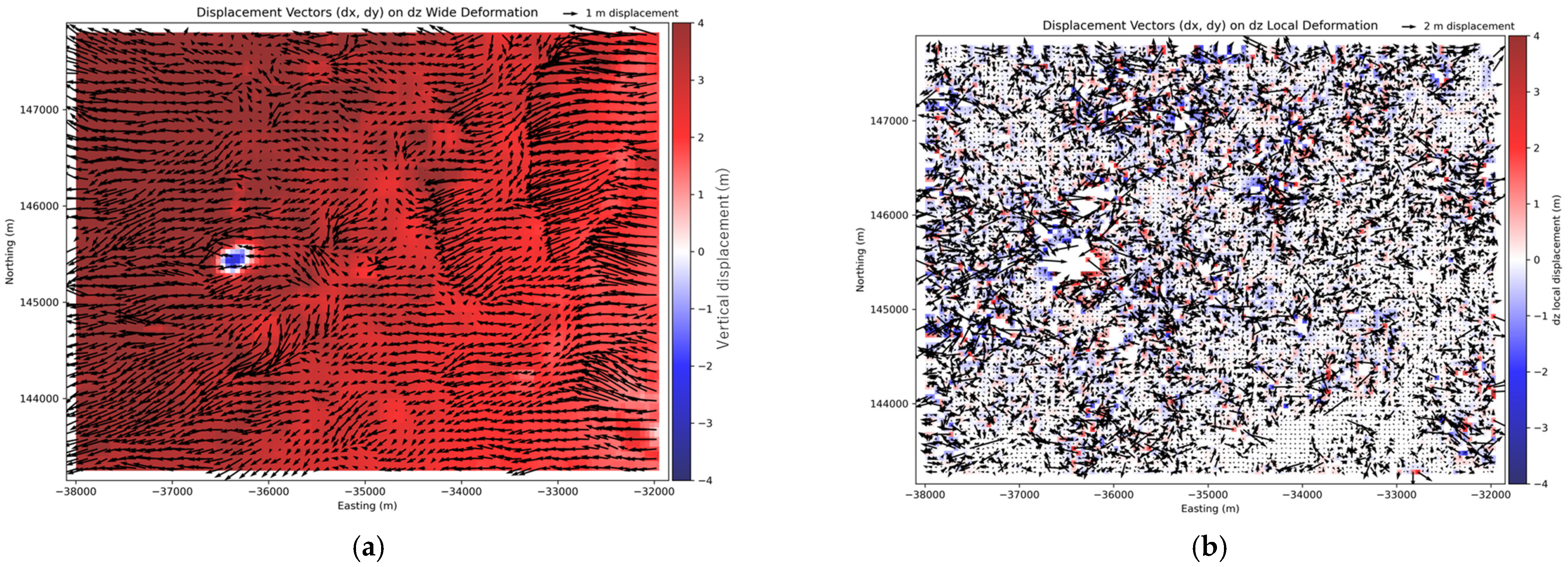
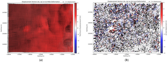
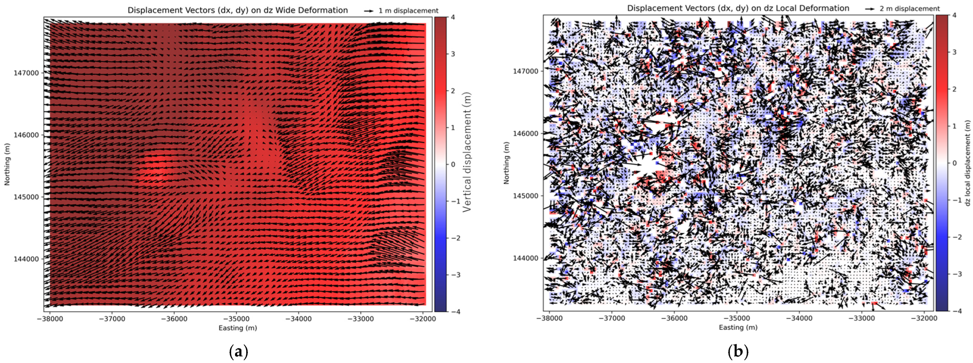
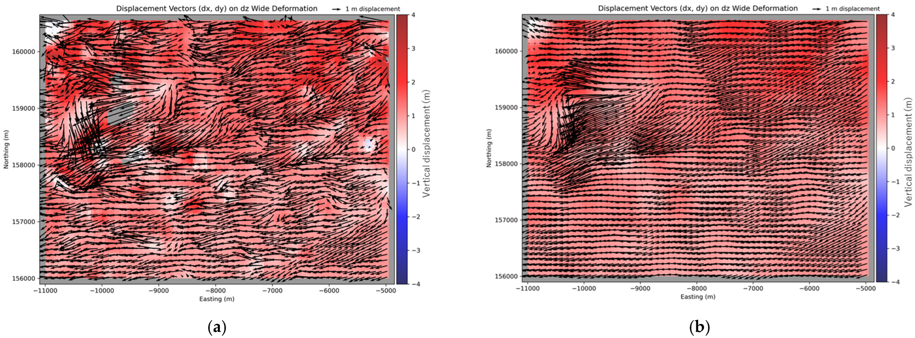
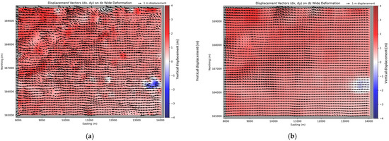
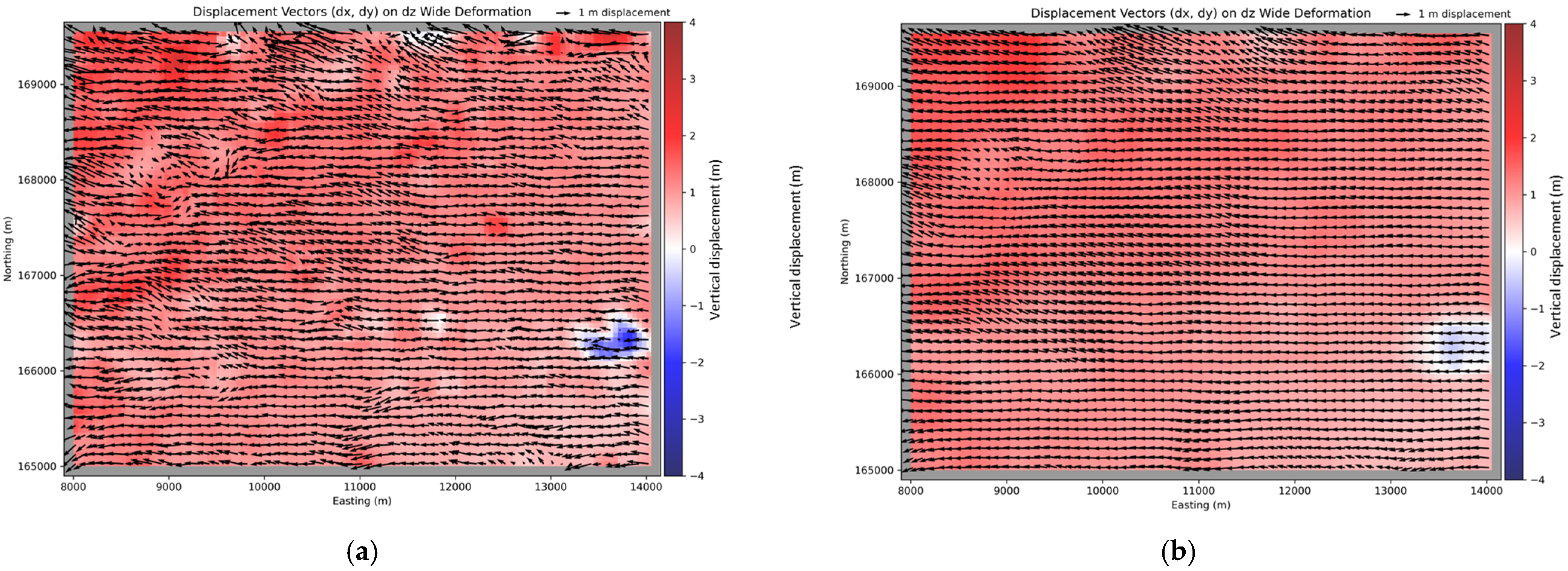
Using the results for the 50 m tiles (windows), the 2D simple moving-average calculation was carried out for various window sizes (k = l = 1, 2, …, 19) using Equation (2). Figure 10 and Figure 11 show the results for a 250 m square (5 × 5) moving window and a 550 m square (11 × 11) moving window, respectively, for the crustal movement (a) and local ground movement (b) components. As the window size increases, the crustal movement becomes smoother for both the horizontal (H) and vertical (V) components. Pixels (50 m tiles) without a solution diminish, and only one sinkhole-like settlement corresponding to the largest landslide remains in the V component for the 250 m moving-window result.

The crustal movement becomes even smoother for the 550 m moving window, and the sinkhole in the V component finally disappears. In contrast, the local soil movement component looks almost the same as that for the 250 m moving-window case, because it consists only of the local residual movements after the removal of the mean trend (crustal movement) component, and the trend is dominant in Monzen. Because the main objective of this study is to extract crustal deformation from the pre- and post-event LiDAR data, further discussion of the local displacement component is deferred to Section 4.2.

The moving-average results for various window sizes (k = l = 1, 2, …, 19) were evaluated using the root mean square error (RMSE) between the GNSS-observed displacement at point i ($d_i^{obs}$) and the displacement estimated by the ICP analysis ($d_i^{est}$) as

$$RMSE=\sqrt{{\displaystyle \frac{1}{n}}{\displaystyle \sum _{i=1}^n}{\left(d_i^{est}-d_i^{obs}\right)}^2}$$

(4)

where n is the number of data points.

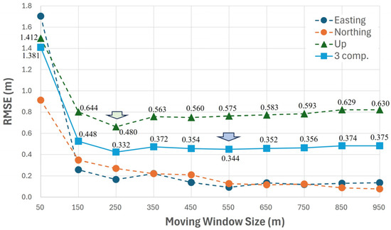
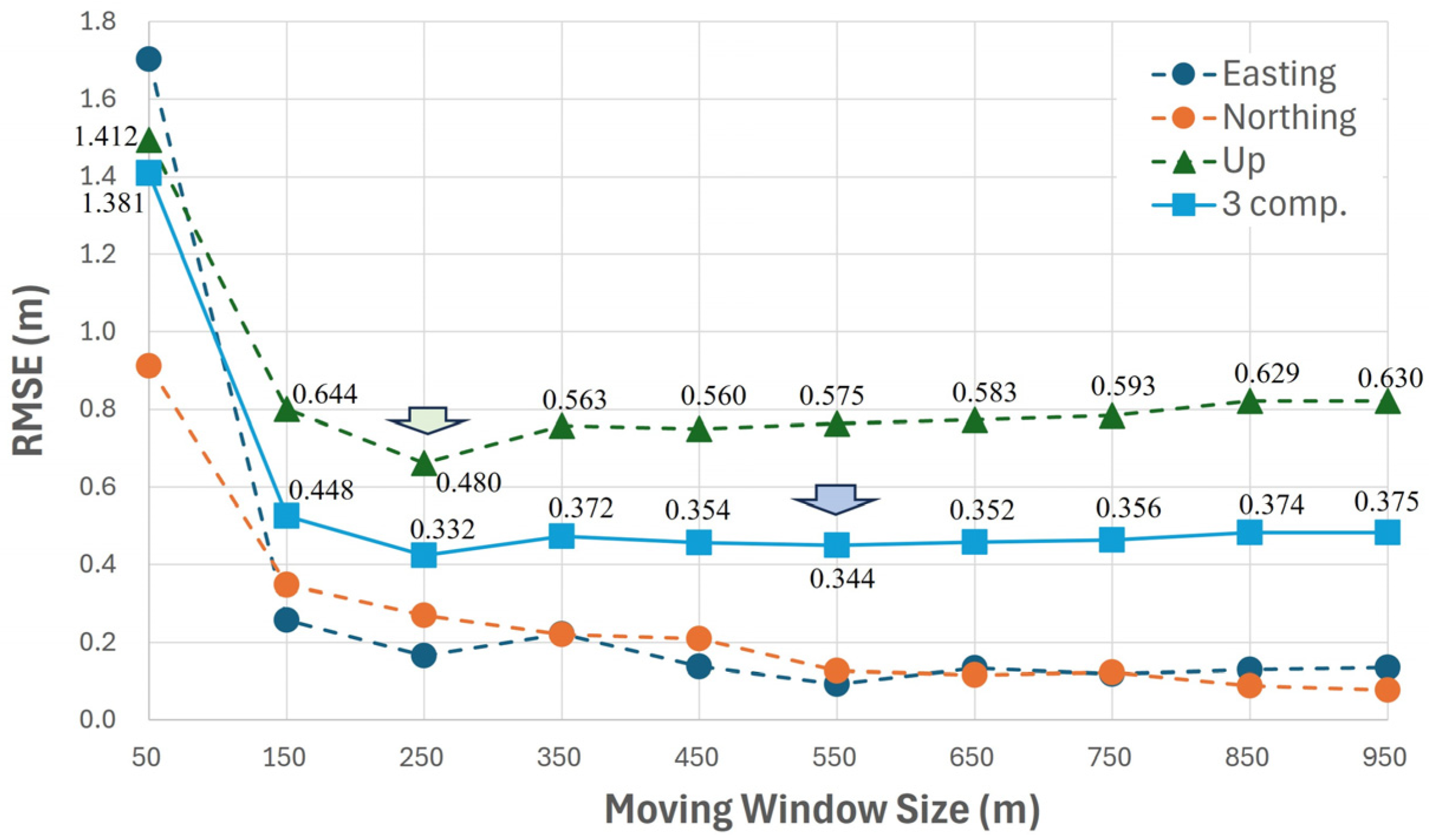
Figure 12 plots the relationship between the moving-window size and RMSE at the five GNSS survey points in Monzen for each direction and for the sum of the three components. The RMSE is smallest for the 250 m window for the three-component sum because uplift is dominant, and the RMSE for the vertical component also reaches its minimum at the 250 m window. In contrast, the RMSE values for the two horizontal components do not show minimum values within this window range (150–950 m) because they are less affected by the local conditions in the study area. The RMSE for the three-component sum shows the second-smallest value at the 550 m window; therefore, the 550 m window is used as another representative size together with the 250 m window hereafter.

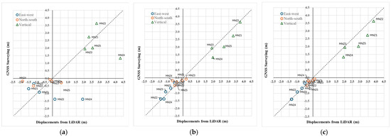
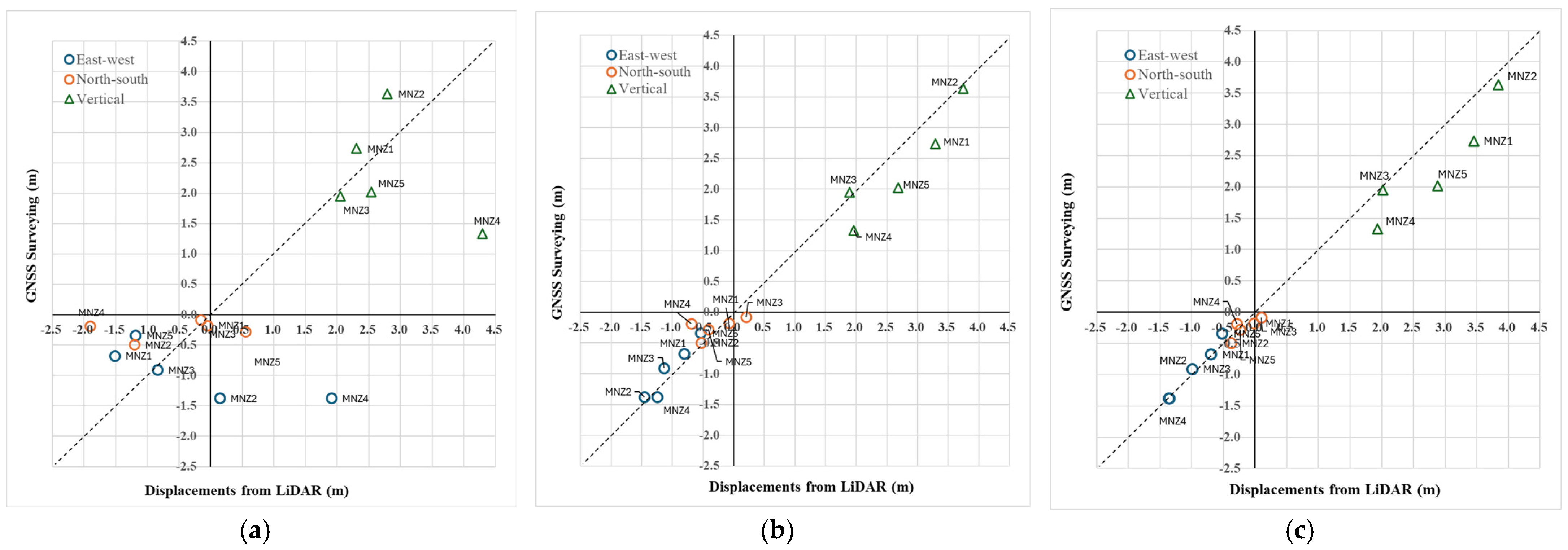
The results for the original 50 m tiles and the moving averages for the 250 m and 550 m windows are compared with the observed displacements at the five survey points in Monzen, as shown in Figure 13 and

Table A2. Observed displacements at GNSS reference points and corresponding ICP-derived results for 50 m × 50 m tiles at 59 sites across 10 study areas on the Noto Peninsula.

Area	Station Name	Station ID	Observed Displacement (m)			ICP Result for 50 m Tiles (m)
			Easting	Northing	Upward	Easting	Northing	Upward
Machino	MCN1	TR45637100601	−1.531	−0.476	1.032	-	-	-
	MCN2	TR45637102601	−1.548	−0.269	1.470	-	-	-
	MCN3	TR45637103601	−1.825	−0.332	1.715	−1.913	−0.938	1.699
Wajima	WJM1	EL05636075102	−1.191	−0.232	1.063	−1.279	−0.556	1.148
	WJM2	TR45636075201	−1.600	0.040	0.713	−1.288	−0.485	0.636
	WJM3	TR45636076001	−1.220	−0.453	1.213	−1.663	−0.635	1.232
Monzen	MNZ1	TR25536769101	−0.672	−0.174	2.735	−1.518	−0.054	2.303
	MNZ2	TR35536755901	−1.374	−0.494	3.638	0.139	−1.210	2.786
	MNZ3	TR35536764201	−0.906	−0.080	1.949	−0.844	−0.162	2.053
	MNZ4	TR35536768401	−1.374	−0.187	1.332	1.904	−1.903	4.294
	MNZ5	TR45536765101	−0.340	−0.280	2.022	−1.190	0.546	2.541
Anamizu	AMZ1	EL05536677201	−0.890	0.222	0.016	−1.051	0.365	0.126
	AMZ2	TR35536676101	−0.910	0.195	0.061	−1.492	0.296	−0.077
	AMZ3	TR35536679001	−1.104	0.139	0.221	−1.145	0.091	0.218
	AMZ4	TR45536666901	−0.937	0.147	0.107	−0.295	0.174	0.678
	AMZ5	TR45536668801	−1.056	0.116	0.193	−1.171	0.206	0.432
	AMZ6	TR45536668901	−1.018	0.136	0.179	−1.151	0.217	0.181
	AMZ7	TR45536669801	−1.183	0.340	0.043	−1.061	0.173	0.250
	AMZ8	TR45536677301	−0.906	0.204	0.038	-	-	-
	AMZ9	TR45536678102	−0.988	0.175	0.113	−1.216	−0.022	0.113
	AMZ10	TR45536770201	−1.074	0.140	0.177	−1.161	0.133	0.241
	AMZ11	TR45536771001	−1.160	0.146	0.192	−1.341	0.115	0.204
Airport	APT1	TR25536775601	−1.177	−0.068	0.240	-	-	-
	APT2	TR35536778801	−1.124	−0.151	0.435	−1.619	−0.211	−0.589
	APT3	TR35537704001	−0.965	−0.009	0.195	−1.007	−0.077	0.247
	APT4	TR45536776801	−1.129	−0.057	0.272	−1.267	0.049	0.424
	APT5	TR45536776901	−1.084	−0.054	0.291	−1.247	−0.031	0.363
	APT6	TR45537706001	−1.027	−0.039	0.259	−1.154	0.017	0.333
Notocho	NTC1	EL05537716101	−0.642	0.207	0.061	−0.898	0.632	−0.011
	NTC2	TR35537706801	−0.701	0.128	0.070	−0.741	0.133	0.260
	NTC3	TR35537709901	−0.800	0.113	0.142	−1.074	−0.191	0.250
	NTC4	TR35637000601	−0.892	−0.018	0.257	−0.952	−0.044	0.270
	NTC5	TR45537706802	−0.697	0.118	0.070	−0.783	0.123	0.190
	NTC6	TR45537708601	−0.808	0.014	0.195	−0.609	0.732	0.321
	NTC7	TR45537708701	−0.793	0.047	0.175	−1.161	0.344	0.251
	NTC8	TR45637001701	−0.931	−0.012	0.274	−0.981	−0.162	0.346
	NTC9	TR45637001801	−0.903	0.042	0.224	−1.193	0.312	0.137
	NTC10	TR45637001901	−0.870	0.098	0.183	−0.430	0.374	0.232
Ogi	OGI1	TR25537718301	−0.606	0.253	0.127	−0.399	0.215	0.310
	OGI2	TR35537718501	−0.564	0.238	0.001	−0.512	0.143	0.044
	OGI3	TR35537718701	−0.509	0.225	−0.003	−0.176	0.348	0.065
	OGI4	TR35637011401	−0.662	0.226	0.050	−0.773	0.982	−0.073
	OGI5	TR45537716401	−0.565	0.247	0.000	−0.100	0.509	0.380
	OGI6	TR45537717701	−0.508	0.232	−0.013	−2.529	0.887	0.090
	OGI7	TR45537719801	−0.522	0.221	0.006	−0.931	0.303	0.093
Horyu	HRY1	TR35637015801	−0.664	0.215	−0.080	−0.776	0.335	0.188
	HRY2	TR35637016501	−0.840	0.238	−0.050	−0.633	−0.138	0.190
	HRY3	TR45637016601	−0.750	0.242	−0.070	−0.455	0.250	0.403
	HRY4	TR45637017601	−0.742	0.132	0.020	−0.433	0.211	0.190
	HRY5	TR45637017701	−0.774	0.234	−0.050	−0.386	0.285	0.228
	HRY6	TR45637018701	−0.772	0.223	−0.040	−1.086	0.390	0.081
	HRY7	TR45637019701	−0.818	0.234	−0.010	−0.890	−0.047	0.257
Suzu	SUZ1	EL05637123103	−0.763	0.008	0.321	−0.097	−0.802	0.081
	SUZ2	TR45637114901	−0.929	−0.004	0.528	-	-	-
	SUZ3	TR45637125301	−0.670	0.062	0.349	2.054	−0.419	−0.097
Noroshi	NRS1	TR35637220301	−1.100	0.117	0.862	−1.372	0.633	0.977
	NRS2	TR35637222001	−1.550	0.610	1.510	−1.396	1.675	1.622
	NRS3	TR45637221401	−1.050	0.221	0.993	−1.620	0.093	1.129
	NRS4	TR45637223201	−1.672	0.917	1.486	−1.824	0.518	1.635

and

Table A3. Moving-averaged ICP-derived displacements from 50 m × 50 m tiles using 250 m and 550 m windows at 59 sites across 10 study areas on the Noto Peninsula.

Area	Station Name	Station ID	250 m Moving Window (m)			550 m Moving Window (m)
			Easting	Northing	Upward	Easting	Northing	Upward
Machino	MCN1	TR45637100601	−1.254	−0.153	0.897	−1.584	−0.284	1.013
	MCN2	TR45637102601	−1.482	−0.102	1.478	−1.155	−0.344	1.445
	MCN3	TR45637103601	−2.247	−0.504	1.660	−2.115	−0.444	1.671
Wajima	WJM1	EL05636075102	−0.746	−0.019	1.110	−1.165	−0.106	1.138
	WJM2	TR45636075201	−1.721	0.045	0.647	−1.393	−0.101	0.617
	WJM3	TR45636076001	−1.582	−0.279	1.202	−1.524	−0.297	1.328
Monzen	MNZ1	TR25536769101	−0.809	−0.073	3.288	−0.697	−0.018	3.449
	MNZ2	TR35536755901	−1.461	−0.528	3.748	−1.364	−0.384	3.835
	MNZ3	TR35536764201	−1.137	0.201	1.897	−0.997	0.097	2.019
	MNZ4	TR35536768401	−1.248	−0.693	1.960	−1.353	−0.292	1.935
	MNZ5	TR45536765101	−0.542	−0.409	2.684	−0.522	−0.239	2.879
Anamizu	AMZ1	EL05536677201	−0.835	0.356	0.093	−0.786	0.289	0.052
	AMZ2	TR35536676101	−1.135	0.349	0.036	−1.022	0.347	0.071
	AMZ3	TR35536679001	−1.159	0.204	0.199	−1.182	0.202	0.205
	AMZ4	TR45536666901	−1.322	0.373	0.230	−0.964	0.358	0.153
	AMZ5	TR45536668801	−1.217	0.204	0.372	−1.129	0.181	0.345
	AMZ6	TR45536668901	−1.184	0.212	0.181	−1.099	0.215	0.193
	AMZ7	TR45536669801	−1.257	0.319	0.281	−1.177	0.263	0.311
	AMZ8	TR45536677301	−1.159	0.210	−0.137	−0.788	0.148	−0.021
	AMZ9	TR45536678102	−1.149	0.140	0.111	−1.028	0.251	0.133
	AMZ10	TR45536770201	−1.174	0.163	0.222	−1.189	0.146	0.235
	AMZ11	TR45536771001	−0.925	0.184	0.271	−1.171	0.170	0.248
Airport	APT1	TR25536775601	−1.317	−0.166	−0.115	−1.192	−0.061	0.003
	APT2	TR35536778801	−1.318	−0.206	0.149	−1.159	−0.132	0.424
	APT3	TR35537704001	−1.020	−0.119	0.320	−1.028	−0.070	0.303
	APT4	TR45536776801	−1.130	−0.077	0.439	−1.123	−0.082	0.378
	APT5	TR45536776901	−0.953	−0.058	0.367	−1.043	−0.059	0.422
	APT6	TR45537706001	−0.974	−0.053	0.437	−0.968	−0.081	0.350
Notocho	NTC1	EL05537716101	−0.726	0.240	−0.096	−0.404	0.322	0.090
	NTC2	TR35537706801	−0.663	0.090	0.204	−0.656	0.104	0.211
	NTC3	TR35537709901	−0.593	0.135	0.170	−0.620	0.077	0.220
	NTC4	TR35637000601	−0.832	−0.018	0.356	−0.751	−0.017	0.339
	NTC5	TR45537706802	−0.369	0.017	0.140	−0.609	0.026	0.143
	NTC6	TR45537708601	−0.779	0.201	0.262	−0.805	0.062	0.266
	NTC7	TR45537708701	−0.665	0.255	0.174	−0.719	0.144	0.204
	NTC8	TR45637001701	−0.928	−0.092	0.374	−0.832	−0.070	0.367
	NTC9	TR45637001801	−0.732	0.038	0.301	−0.909	0.039	0.324
	NTC10	TR45637001901	−0.472	−0.019	0.318	−0.458	0.031	0.254
Ogi	OGI1	TR25537718301	−0.671	0.193	0.228	−0.716	0.250	0.142
	OGI2	TR35537718501	−0.346	0.239	0.033	−0.372	0.308	−0.009
	OGI3	TR35537718701	−0.616	0.340	0.009	−0.608	0.393	0.043
	OGI4	TR35637011401	−0.548	0.530	0.188	−0.442	0.272	0.152
	OGI5	TR45537716401	−0.438	0.416	0.106	−0.371	0.349	0.044
	OGI6	TR45537717701	−0.401	0.456	0.095	−0.485	0.406	0.062
	OGI7	TR45537719801	−0.546	0.503	0.077	−0.597	0.459	0.106
Horyu	HRY1	TR35637015801	−0.780	0.252	0.151	−0.698	0.272	0.138
	HRY2	TR35637016501	−0.835	0.075	0.057	−0.672	0.120	0.160
	HRY3	TR45637016601	−0.718	0.365	0.357	−0.713	0.343	0.262
	HRY4	TR45637017601	−0.652	0.172	0.189	−0.585	0.256	0.156
	HRY5	TR45637017701	−0.568	0.259	0.162	−0.677	0.223	0.133
	HRY6	TR45637018701	−0.718	0.259	0.156	−0.606	0.113	0.152
	HRY7	TR45637019701	−0.616	0.019	0.277	−0.650	0.136	0.250
Suzu	SUZ1	EL05637123103	−0.474	−0.168	0.258	−0.765	−0.056	0.209
	SUZ2	TR45637114901	−0.869	−0.236	0.599	−0.842	−0.076	0.622
	SUZ3	TR45637125301	0.259	−0.183	0.122	−0.101	−0.012	0.204
Noroshi	NRS1	TR35637220301	−1.195	0.170	1.040	−1.050	0.236	1.119
	NRS2	TR35637222001	−1.861	0.594	1.586	−1.545	0.348	1.606
	NRS3	TR45637221401	−1.239	0.061	1.141	−1.001	0.091	1.141
	NRS4	TR45637223201	−1.586	0.691	1.439	−1.424	0.380	1.300

. For both window sizes, the two horizontal displacement components agree well with the observed values (RMSE < 0.2 m, as also shown in Figure 12), whereas the 50 m tile results exhibit much greater scatter. For the vertical component, however, good agreement is seen at points MNZ2 and MNZ3 for both the 250 m and 550 m moving windows, whereas overestimation of more than 0.5 m is observed at the other three points. This discrepancy is discussed in Section 4.2.

3.2. The 3D Crustal Movement in Anamizu Town

The ICP analysis of the pre- and post-event LiDAR DEM data for 50 m tiles and the moving-average analysis based on these 50 m tile results were also tested in Anamizu Town, where the vertical coseismic displacements (uplift) were much smaller than those in Monzen but the horizontal displacements exceeded 1 m westward. There are 11 survey control points (one GEONET station and 10 triangulation points) in the study area shown in Figure 2—the largest number of GNSS reference points among the 10 selected study areas.

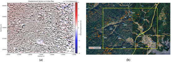
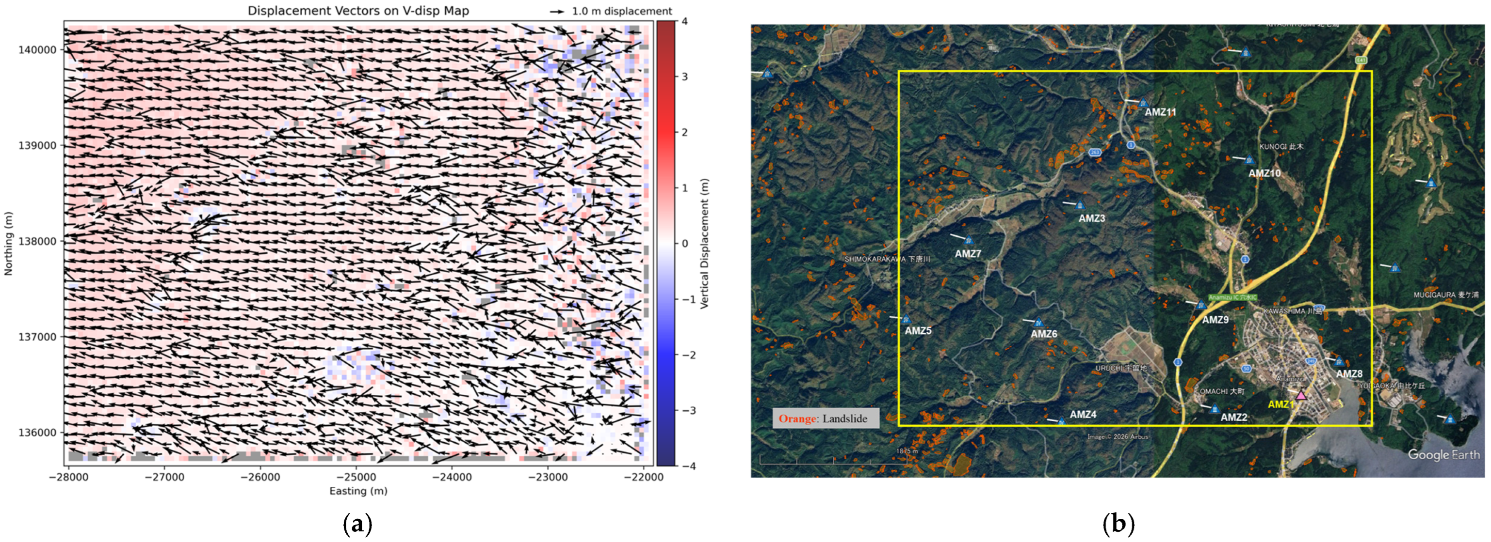
Figure 14a shows the ICP analysis result for 50 m DEM tiles in the Anamizu study area (6.0 km × 4.5 km): vertical displacements are shown by the colors of the 50 m tiles, and horizontal displacements are shown by arrows at 100 m spacing. The vertical displacements are clearly much smaller than those in Monzen, with a maximum value of about 0.2 m. The horizontal displacements are more uniform in both amplitude and orientation than those in Monzen. The landslide polygons [38] are shown in Figure 14b, together with the 11 GNSS survey control points in the study area. Some landslide-affected zones also exist in Anamizu along roadways and in forests, but they are much fewer than those in Monzen.

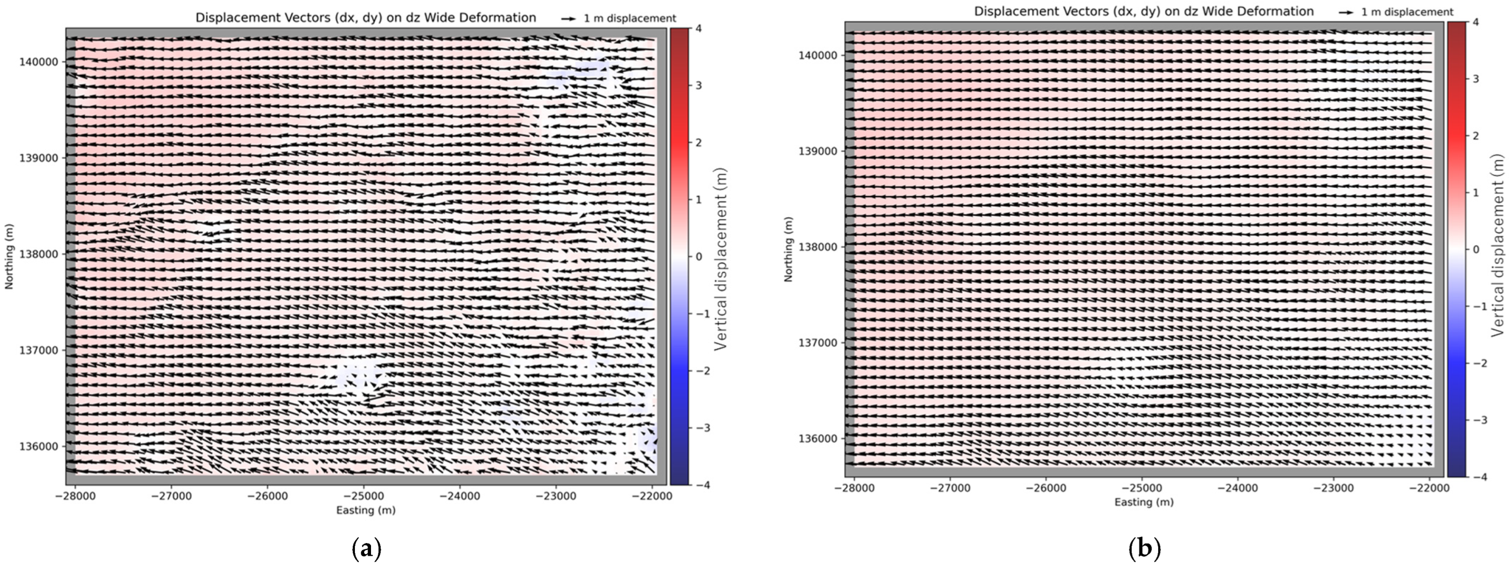
Figure 15 shows the moving-average results for the 250 m square (5 × 5) moving window and the 550 m square (11 × 11) moving window. Both the horizontal and vertical displacements become more stable as the window size increases, as expected from Figure 14.

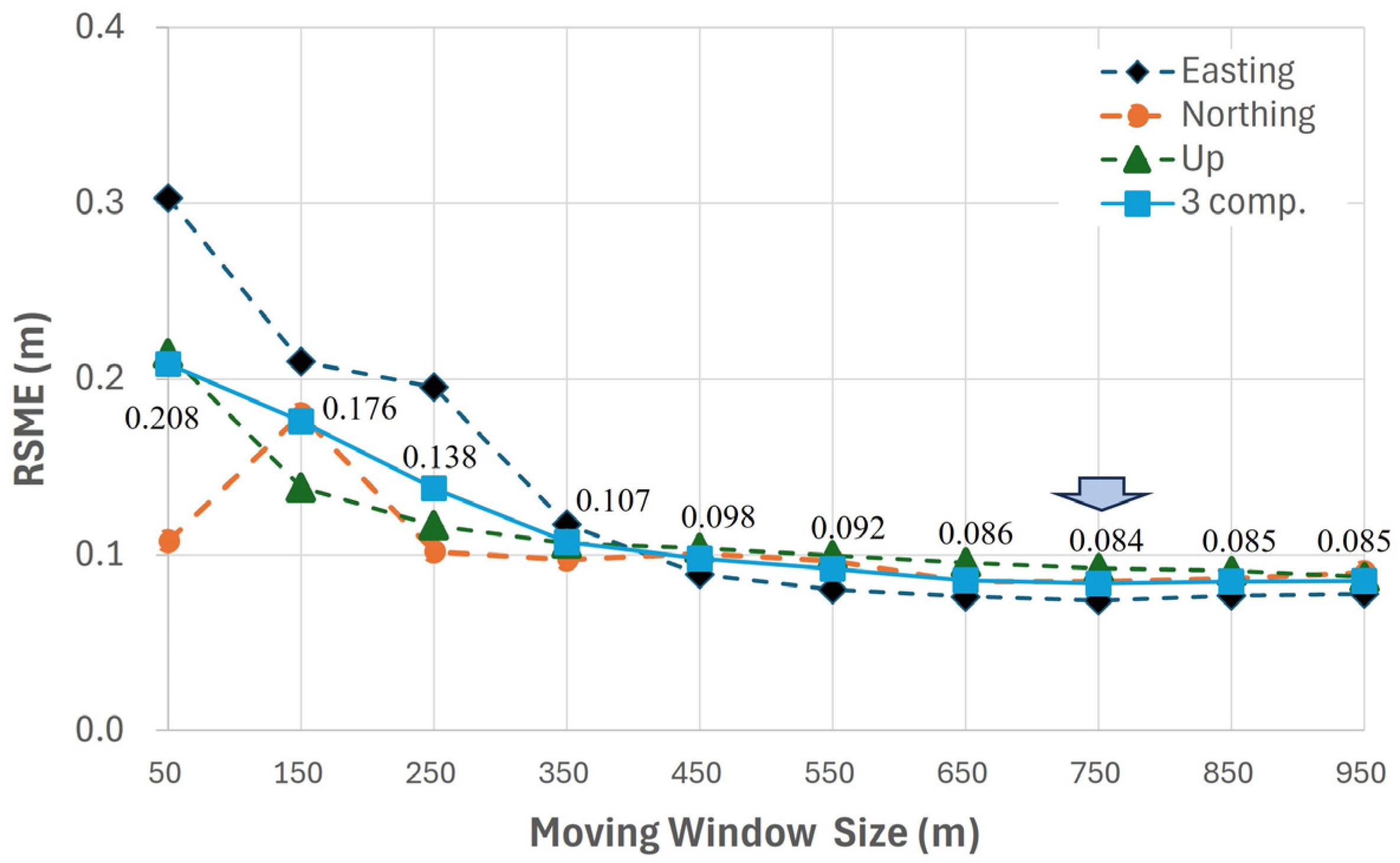
The moving-window size was also examined in Anamizu, as shown in Figure 16, which plots the variation in the RMSE for the 11 GNSS observation points with respect to the window size. The RMSE values are much smaller for each direction and for the sum of the three components. The RMSE for the three-component sum reaches its minimum at the 750 m moving window, but it changes very little and remains below 0.1 m for window sizes larger than 350 m. This observation confirms the validity of the moving-average scheme for ICP analysis with a smaller tile size.

Comparing Figure 12 and Figure 16, the most appropriate moving-window size appears to depend on the ground-surface conditions and the magnitude and spatial variability of the coseismic deformation. Areas with extensive landsliding and surface disruption, such as Monzen, may require larger windows to obtain stable displacement estimates, whereas relatively stable areas, such as Anamizu, may be better represented by different window sizes. Therefore, the window sizes identified in this study should not be regarded as universally applicable values. Furthermore, because the same GNSS dataset contributed both to window size selection and to the subsequent accuracy assessment, the reported RMSE values should be interpreted as indicative rather than fully independent validation results. Additional case studies from different earthquake environments and independent validation datasets will be required to establish more general criteria for selecting appropriate moving-window sizes.

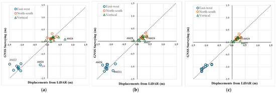
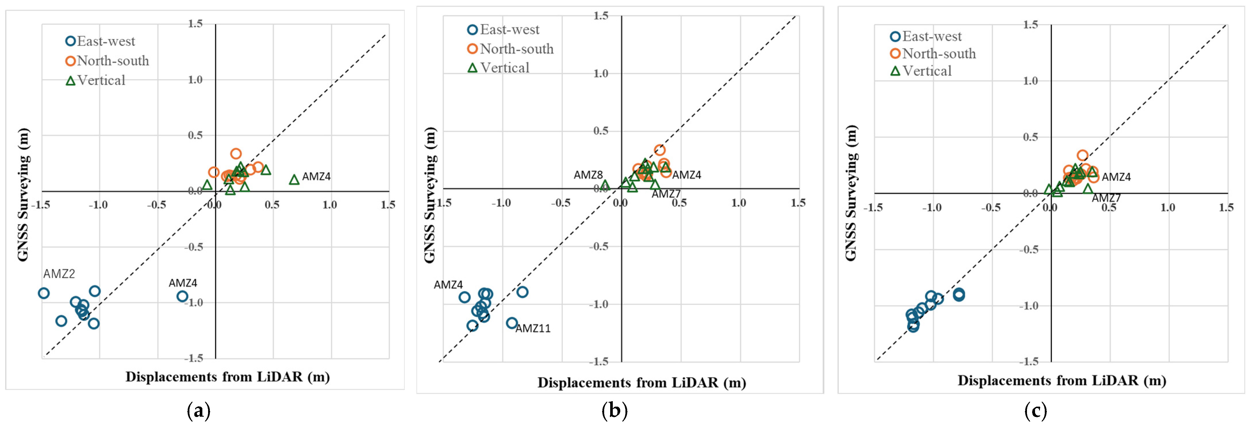
The results for the original 50 m tiles and the moving averages for the 250 m and 550 m windows are compared with the observed displacements at the 11 GNSS reference points in Anamizu, as shown in Figure 17 and Table A2 and Table A3. The 50 m tile results exhibit errors greater than 0.5 m in the EW and UD directions. The EW components still show some errors (AMZ4 and AMZ11) for the 250 m window, but these errors become much smaller for the 550 m window. For the 550 m moving window, the maximum error is 0.21 m for the NS component at AMZ4 and 0.27 m for the vertical component at AMZ7. These results further support the effectiveness of the moving-average scheme for estimating crustal movements from airborne LiDAR data.

3.3. The 3D Crustal Movement in Machino District, Wajima City

As the third study area for extracting coseismic displacements from airborne LiDAR data, the Machino district in the eastern part of Wajima City was selected because its crustal deformation was the second largest after Monzen and slope failures were frequent, as shown in Figure 1 and Figure 2.

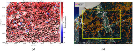
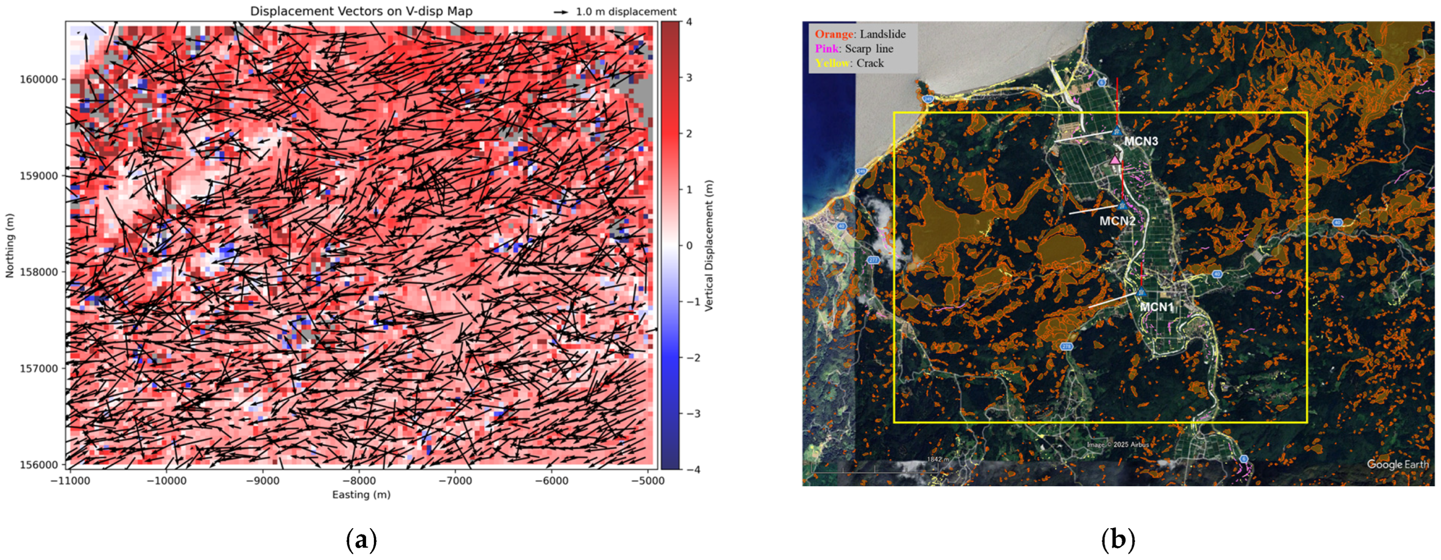
The result of the ICP analysis for 50 m DEM tiles in the Machino study area (6.0 km × 4.5 km), together with an optical satellite image (Google Earth) showing the ground-failure locations and three survey control points, is presented in Figure 18. The vertical displacement (uplift), shown by color, is smaller than that in Monzen but much larger than that in Anamizu. There are some gray pixels (50 m tiles) without solutions and some white/blue pixels indicating settlement. These irregular pixels correspond to landslide-related polygons in forested areas [38]. Two additional types of ground-surface irregularity data are also shown: scarp lines [38], indicated by pink lines, and surface cracks [51], indicated by yellow lines. The scarp lines are mainly observed in cropland, whereas the cracks occur along river and road embankments.

Figure 19 shows the moving-average results for the 250 m and 550 m windows. Owing to the effect of moving averaging, the irregular areas in the original 50 m tile results become smoother as the window size increases. However, in this study area, nonuniform crustal movements still remain even within this window range.

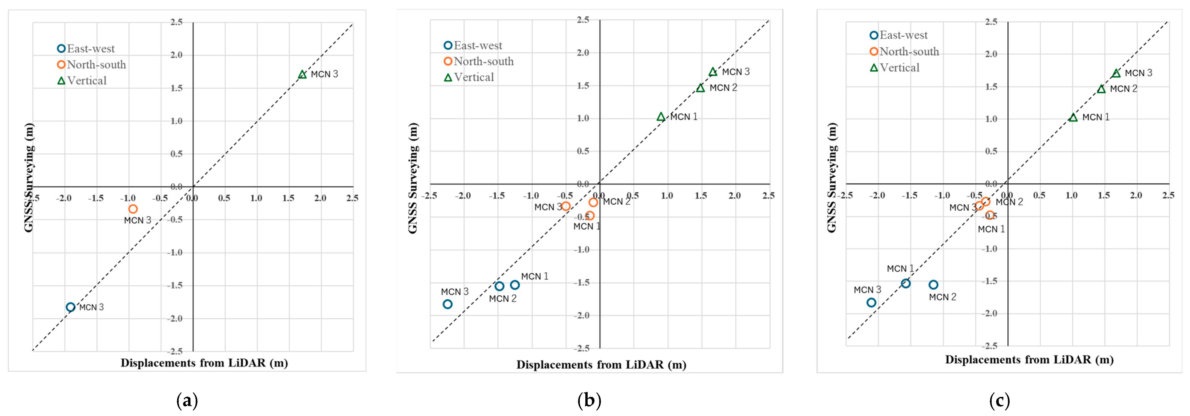
The results for the original 50 m tiles and the 250 m and 550 m moving windows are compared with the observed displacements at the three reference points in Machino, as shown in Figure 20 and Table A2 and Table A3. The ICP analysis for the original 50 m tiles could not provide meaningful results (less than 5.0 m for each horizontal direction) at MCN2 and MCN3, probably because of soil surface irregularity around these points. However, the moving-average calculation yielded meaningful results for larger window sizes. The estimated vertical displacements almost perfectly match the GNSS observations after moving averaging. The deviations in the estimated horizontal displacements for the 250 m window become smaller for the 550 m window. In spite of the ground irregularity near the control points, the proposed calculation scheme is considered effective for reducing errors.

3.4. The 3D Crustal Movement in Noroshi District, Suzu City

As the fourth study area for crustal deformation, the Noroshi district at the northeastern tip of the Noto Peninsula in Suzu City was selected because seafloor uplift was large there and the epicenter was located nearby. The earthquake swarm had continued in this area from late 2020 until the main shock occurred at 16:10:22.5 JST on 1 January 2024 [32].

The result of the ICP analysis for 50 m DEM tiles in the Noroshi study area, together with an optical satellite image showing the ground-failure locations [38,51] and four GNSS survey points, is shown in Figure 21. To select a square area of 6.0 km × 4.5 km that included as many GNSS points as possible, the current layout was adopted even though it included some sea areas. These sea areas correspond to no-data (gray) or zero-vertical-displacement (white) pixels. A group of blue pixels in the southeastern part of the study area corresponds to a dam reservoir; therefore, the negative values there indicate a reduction in water level rather than ground settlement due to the earthquake.

Figure 22 shows the moving-average results for the 250 m and 550 m windows. The irregular areas in the original 50 m tile results become smoother as the window size increases. The effects of the sea and reservoir are reduced by the moving-average calculation, but they still remain even for the 550 m window case. The displacement field could be improved by excluding water bodies such as reservoirs and coastal waters prior to smoothing. However, the reliable identification of such areas generally requires auxiliary datasets, including contemporaneous optical imagery or land cover information, which may not be available immediately after a disaster. Therefore, no additional masking procedure was applied in this study, and the resulting displacement maps should be interpreted with caution in water-covered areas.

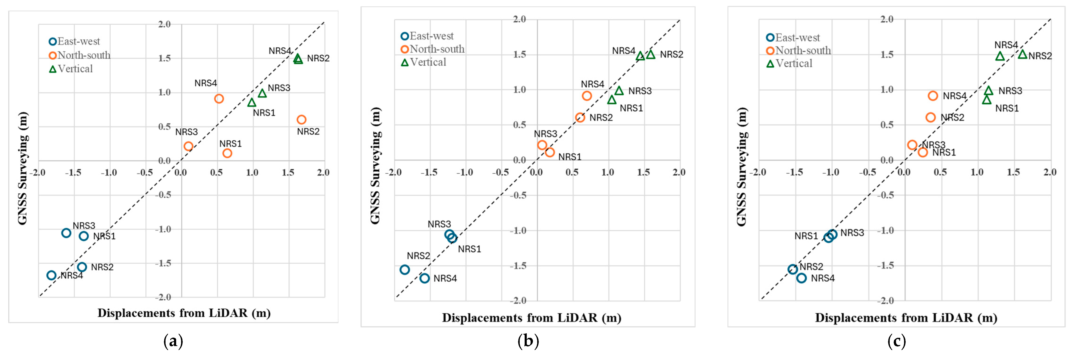
The results for the original 50 m tiles and the moving averages for the 250 m and 550 m windows are compared with the observed displacements at the four reference points in Noroshi, as shown in Figure 23 and Table A2 and Table A3. The scattered values for the NS displacement in the original 50 m tiles become closer to the reference data after moving averaging.

However, errors still remain in the NS component at NRS2 and NRS4, both of which are located close to sea cliffs. Slope failures were observed within 50 m of NRS2, which might generate errors in the ICP analysis and moving average calculation. Seafloor uplift occurred along the coast line in the study area. NRS4 is located 150 m south of the coast, and this position might affect the moving average calculation.

3.5. The 3D Crustal Movement for the 10 Study Areas with 59 GNSS Observation Points

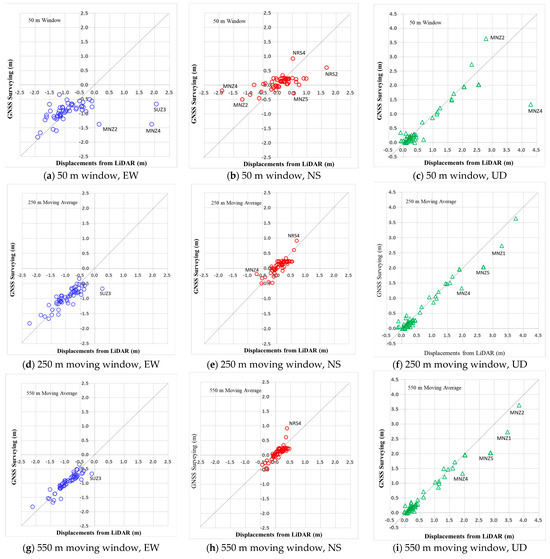
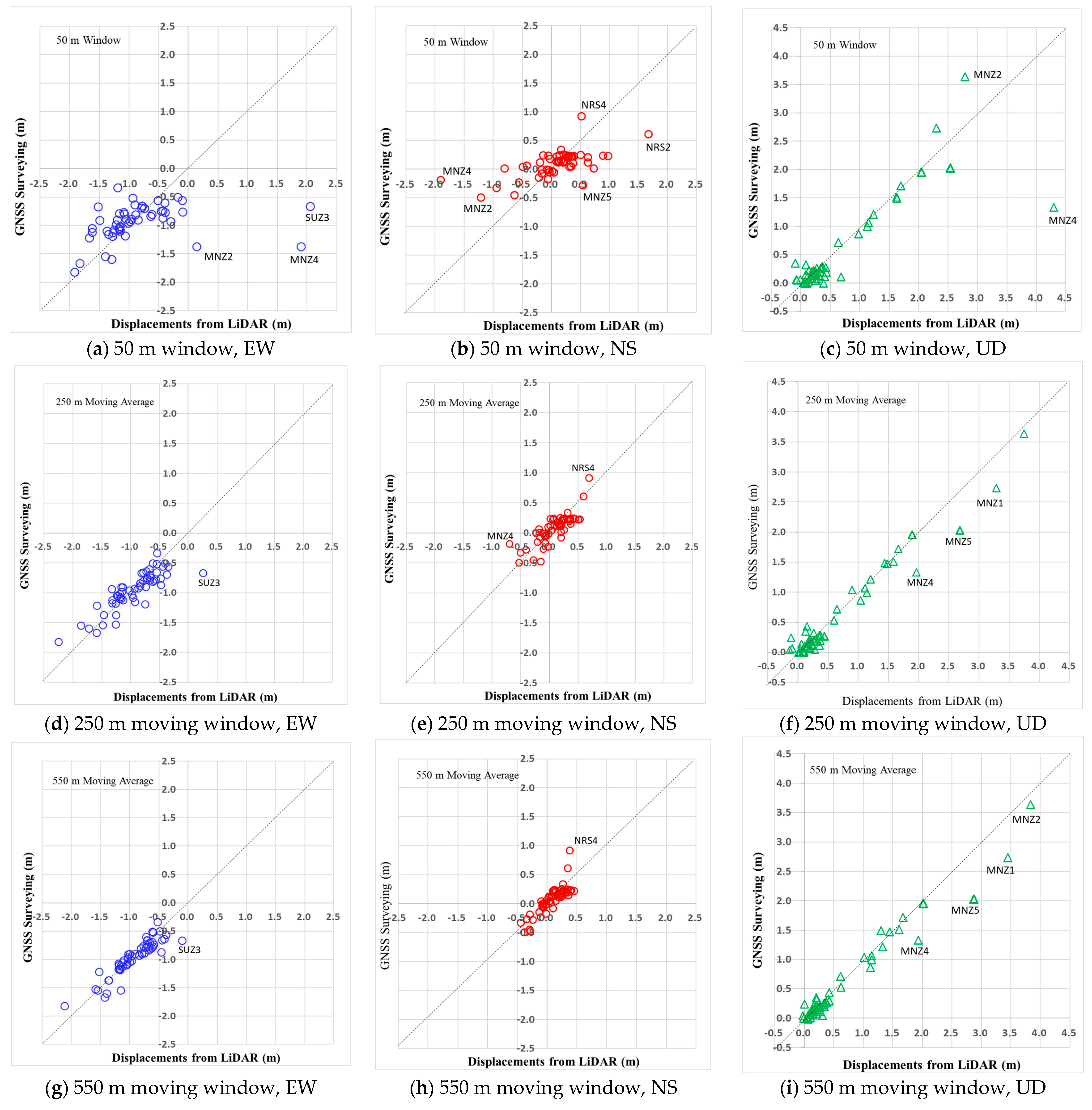
In the same manner as for the four study areas described above, 3D coseismic displacements were also calculated for six additional study areas shown in Figure 2. The results for the 10 study areas, including a total of 59 GNSS survey points provided by the GSI, are summarized in Figure 24 and Table A2 and Table A3. The corresponding RMSE values for the 59 survey points are listed in

Table 2. RMSEs of analysis results at 59 GNSS reference points across 10 study areas.

Window	50 m Original Tile			250 m Moving Average			550 m Moving Average
Direction	EW	NS	UD	EW	NS	UD	EW	NS	UD
RMSE (m)	0.746	0.430	0.477	0.222	0.156	0.183	0.158	0.127	0.193
RMSE for Three Components (m)	0.551			0.187			0.159

for the original 50 m tiles and the 250 m and 550 m moving averages. The RMSE for the sum of the three components decreases from 0.55 m for the 50 m tiles to 0.19 m for the 250 m moving average and 0.16 m for the 550 m moving average. The coseismic displacements were much smaller and slope failures were less frequent in the study areas facing Toyama Bay and Nanao Bay.

The ICP and moving-average results for the remaining six study areas (Wajima City Center, Noto Airport, Notocho Town Center, Ogi District, Horyu District, Suzu City Center) shown in Figure 2 are provided in the Supplementary Materials.

4. Discussion

4.1. Data Type of Airborne LiDAR for the Extraction of Coseismic Displacements

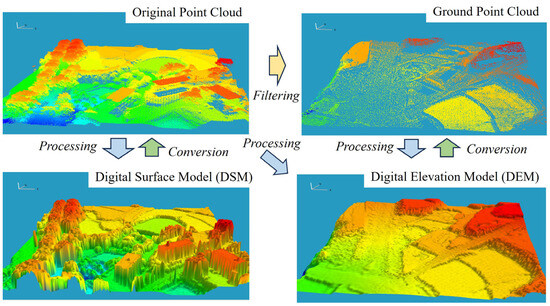
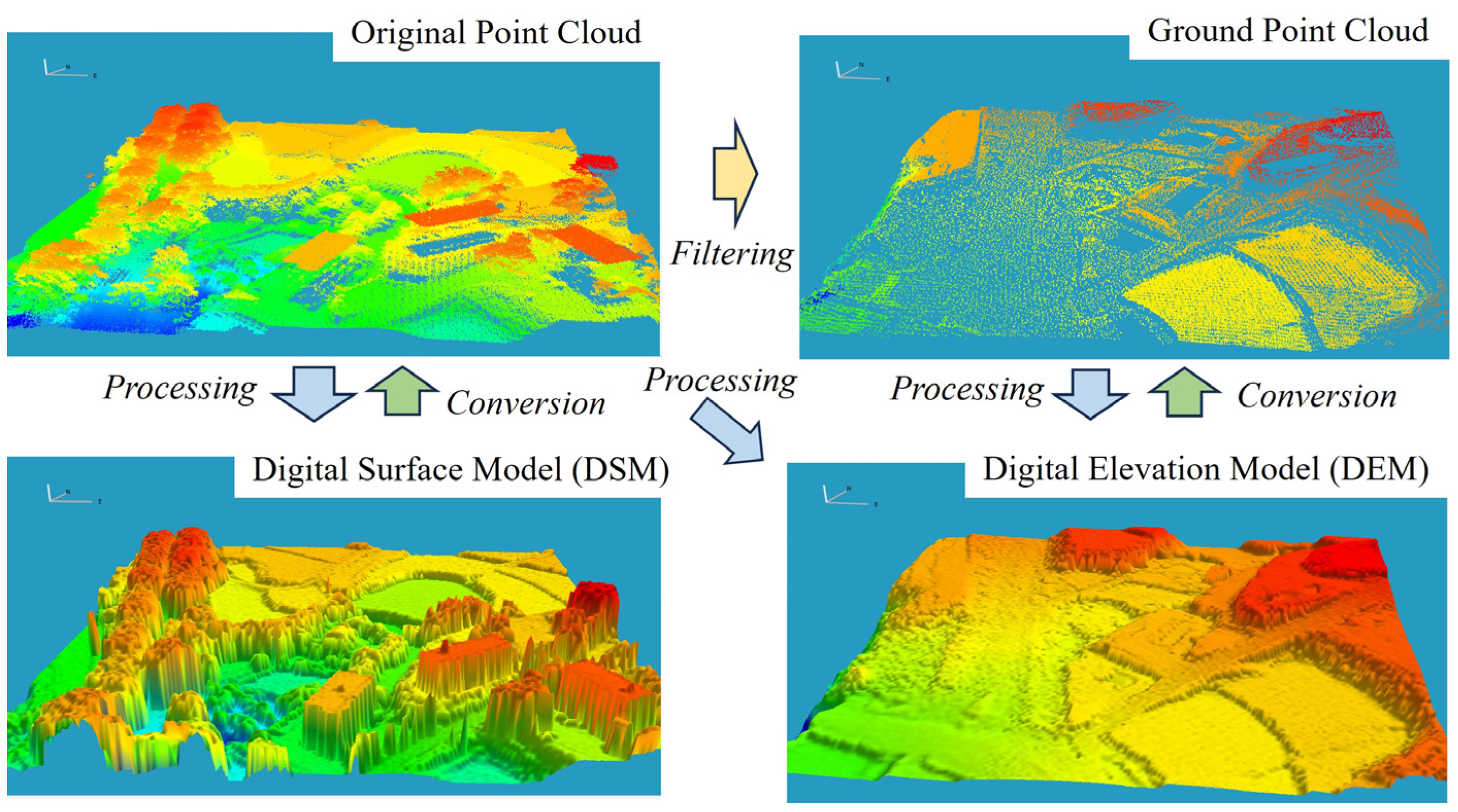
Airborne LiDAR data are available in several forms, as shown in Figure 25. Raw observations are recorded as original point clouds in xyz coordinates, including all objects on the ground surface, such as trees, buildings, bare ground, and poles. Ground (terrain) point clouds are then obtained by cleaning and filtering nonground objects from the raw data. Digital surface models (DSMs) and digital elevation (terrain) models (DEMs/DTMs) are generated from original point clouds and ground point clouds, respectively. Both DSMs and DEMs can be produced either as triangular irregular networks (TINs) or in raster (grid) form [52].

In our case study of the 2024 Noto Peninsula earthquake, the pre-event data were available as original point clouds, whereas the post-event data were available as DEMs with a 0.5 m grid. Therefore, we first produced ground point clouds from the original point clouds and then generated the DEMs using the ENVI LiDAR software (version 6.1). To perform the ICP analysis with the Python program [49], the pre- and post-event DEMs were converted back to LAS-format point clouds after selecting the common study area. Because of this data limitation, we used only DEMs (ground point clouds). However, if the original point-cloud data for both epochs were available, ICP analysis could also be performed on DSMs (or the original point clouds).

An important question is which data type—DSMs or DEMs—is more suitable for obtaining coseismic displacements from a pair of pre- and post-event LiDAR datasets. In our experience with LiDAR differencing for the 2018 Hokkaido–Iburi earthquake [53], DEMs represented coseismic ground displacements better than DSMs because DSMs included tree growth and forestry activities that occurred during the time interval between the two datasets.

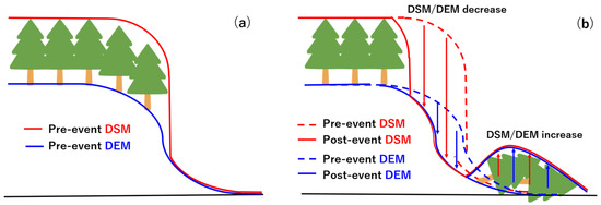
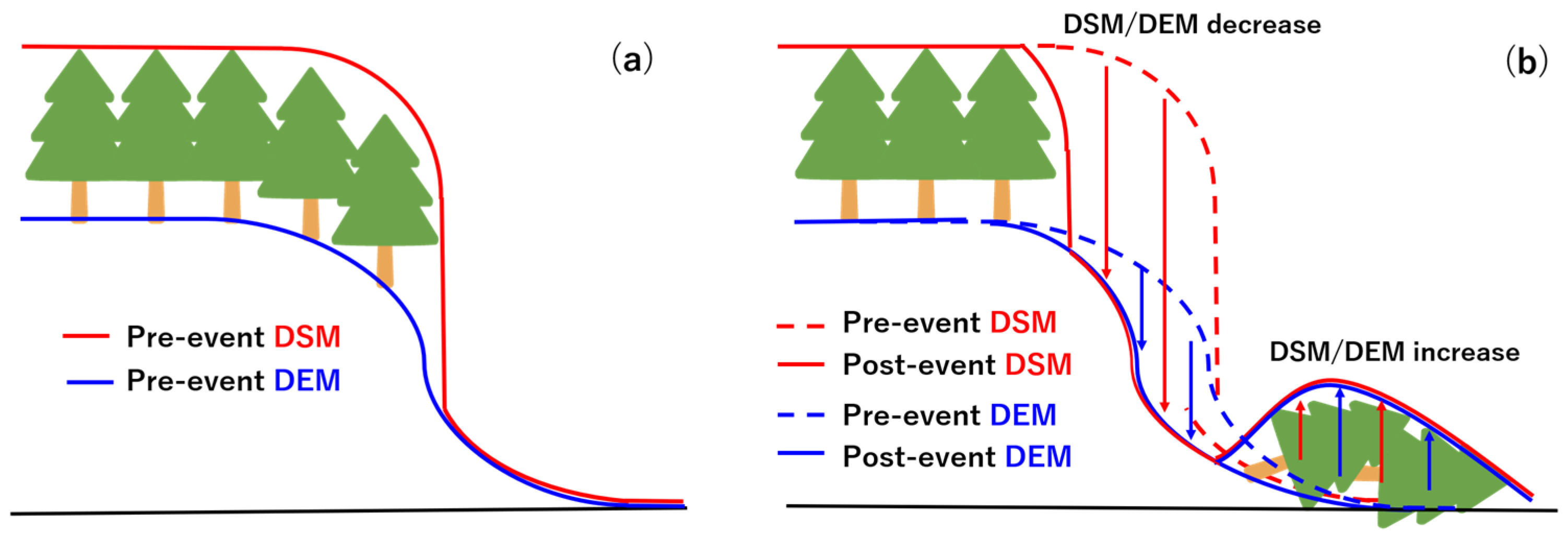
Fallen trees and collapsed buildings caused by earthquakes also introduce errors in change detection because they might be recognized as ground rather than as above-ground objects, as illustrated schematically in Figure 26. Landslides and associated fallen trees may cause the overestimation of ground-surface elevation [54]. However, when there is little or no time lag between the two LiDAR acquisitions, DSMs can provide better coseismic displacement estimates, especially in urban areas [47], because buildings and urban infrastructure serve as good markers for cross-correlation between the DSMs.

4.2. Effects of Ground Failures on Crustal Deformation and Local Displacements

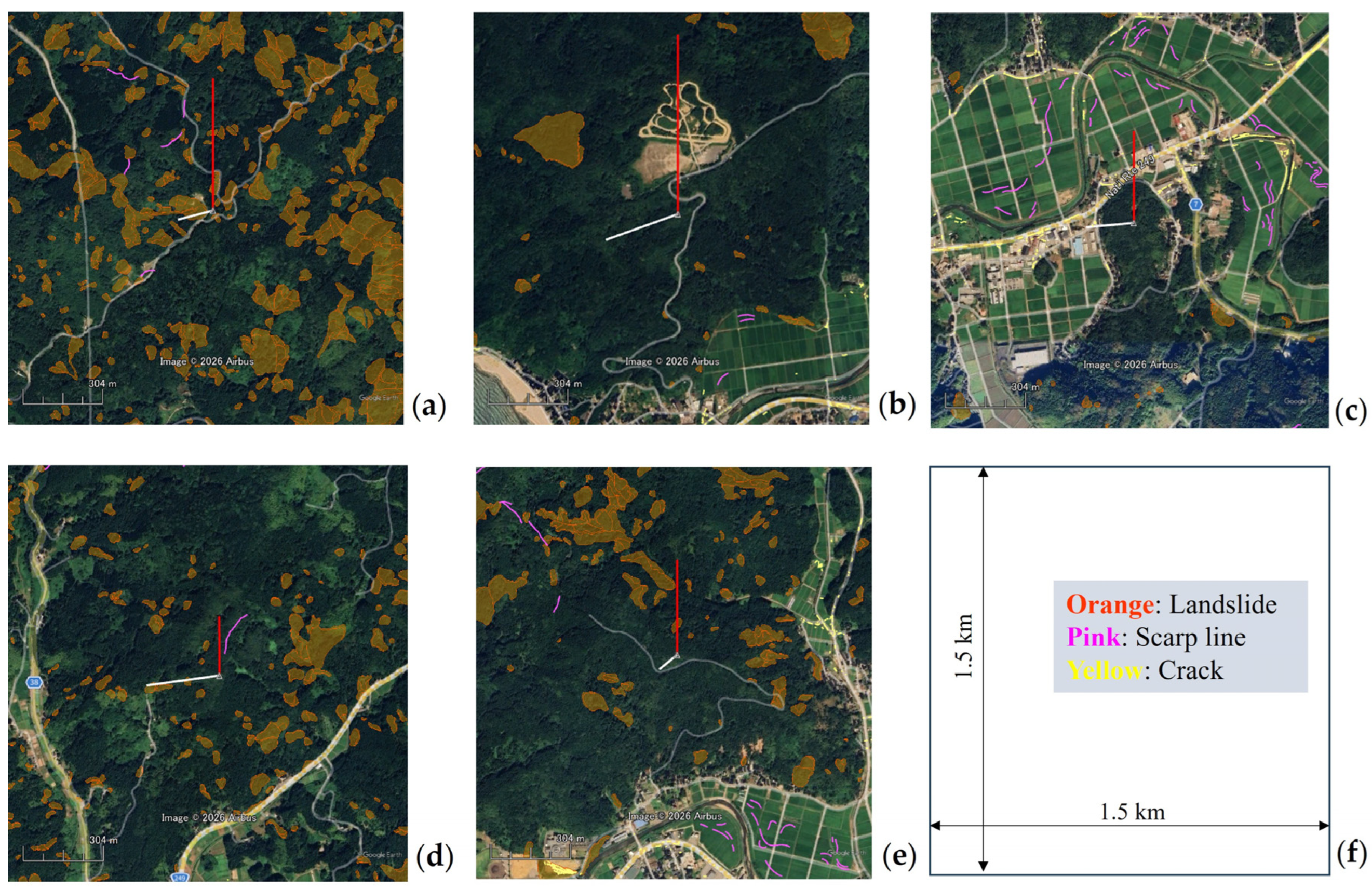
As shown in Figure 24, the proposed method in this study—ICP analysis for 50 m tiles combined with moving-average windows—provided accurate results for the 59 reference points in the 10 study areas on the Noto Peninsula. Some results for the 50 m tiles, however, contain considerable errors, especially in the two horizontal components. Almost all of these errors diminish after the moving-average operation. For the vertical component, however, errors of 0.7–0.8 m still remain in the Monzen area, where the upward crustal movements were largest during the event. To investigate the cause of the vertical errors, optical images of the surrounding 1.5 km square areas around the five GNSS reference points in Monzen are presented in Figure 27, together with visible ground failures (landslide polygons and scarp lines [38] and cracks [51]) identified from the LiDAR data and aerial photographs. At MNZ1, MNZ4, and MNZ5, where the vertical component errors are large, landslide zones are recognized within 150 m of the triangulation points. As discussed before, landslides and fallen trees may cause the overestimation of DEMs. The errors in the vertical component at these three sites can be explained by this mechanism.

The physical meaning of the local displacement components in Equations (1)–(3) was further examined for the Monzen area. Figure 28 compares the local displacement components obtained using the 550 m moving window (Figure 11b) with the mapped landslide polygons (Figure 9b [38]). The vertical local displacement shows some correspondence with the landslide locations, although small patches of colored pixels are also observed between the landslide polygons. In contrast, the horizontal local displacement is distributed rather randomly across the study area. Horizontal local displacements could not be estimated within large landslide areas. The horizontal displacement vectors appear to be oriented downslope in the mountainous regions, whereas they are relatively small on the flat terrain along the major road in the southern part of the study area.

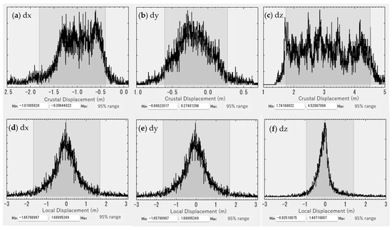
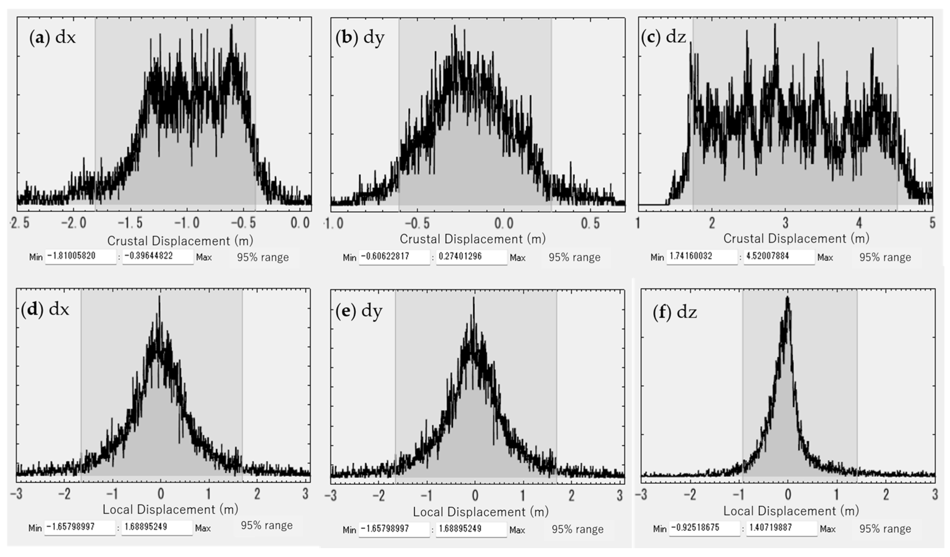
Histograms of the crustal deformation components and local displacement components for the Monzen area are shown in Figure 29. A clear distinction can be observed between the crustal deformation components (mean trend) and the local displacement components (residuals). The former exhibit a broad range of displacement values while maintaining a consistent orientation (westward, predominantly southward, and upward). In contrast, the latter are approximately centered on zero and resemble a Gaussian distribution. These distinct distribution patterns suggest that the decomposition into crustal deformation and local displacement components has physical significance, effectively separating the long-wavelength crustal deformation signal from the mixed ICP-derived displacements.

4.3. Ground-Based GNSS Observation vs. Airborne LiDAR Data

In this study, pre- and post-earthquake high-density airborne LiDAR data were used to estimate three-dimensional coseismic displacements associated with the 2024 Noto Peninsula earthquake. Ground-based GNSS observations at 59 locations were used to validate the ICP-derived results. In addition, 154 survey reference points with pre- and post-event GNSS observations are available in the upper part of the peninsula (Figure 2). Because the density of observation points is relatively high in the southern Noto Peninsula, facing Nanao Bay and Toyama Bay, spatial interpolation of the 154 GNSS displacement measurements for each component (EW, NS, UD) can be performed directly without relying on physical models.

Although the displacement fields derived from airborne LiDAR data may appear less smooth than those interpolated from ground-based GNSS observations, this difference reflects fundamental distinctions in measurement characteristics. Airborne LiDAR captures spatially dense surface changes, including localized deformation associated with ground failures, whereas GNSS observations represent discrete points anchored to relatively stable ground and are typically interpolated to produce smoother displacement fields.

In areas affected by landslides, lateral spreading, and other surface instabilities, GNSS-based displacements may be influenced by local effects depending on the station location. In contrast, the LiDAR-based approach enables the identification of such localized deformation patterns at a much finer spatial resolution. The apparent ambiguity observed in the LiDAR-derived displacements is therefore partly attributable to the inclusion of real, small-scale deformation signals rather than measurement noise.

Regarding data availability, GNSS observations at triangulation points were released approximately 1.5 years after the earthquake and were therefore not available for rapid post-event analysis. In contrast, airborne LiDAR data were acquired within a few months after the event, highlighting the practical advantage of the proposed approach for early-stage earthquake response and recovery.

Continuously operating reference stations (CORSs) are not yet sufficiently dense, even in a relatively small and densely populated country such as Japan. Therefore, satellite SAR systems remain essential for measuring crustal deformation over wide areas associated with earthquakes and volcanic activity. Airborne LiDAR observations are expected to serve as an intermediate-scale bridge between CORSs (high-accuracy point measurements) and satellite SAR (broad spatial coverage). Although ALOS-2 pixel-offset results are available for the Noto Peninsula earthquake, quantitative validation against these products was not possible because the corresponding digital displacement data were not publicly available.

5. Conclusions

In this study, three-dimensional (3D) ground-surface displacements were estimated using airborne LiDAR data acquired before and after the 2024 Noto Peninsula earthquake. Digital elevation models (DEMs) were generated from pre-earthquake point cloud data acquired by Ishikawa Prefecture and compared with post-earthquake DEMs developed by the Forestry Agency of Japan. Three-dimensional coseismic displacements were derived from the spatial correlations between the pre- and post-event DEMs for 50 m × 50 m tiles using the Iterative Closest Point (ICP) algorithm.

The calculation results depend on the tile size and are influenced by the amplitude and spatial distribution of coseismic ground movements. Therefore, moving-average windows of 250 m and 550 m were applied to the 50 m tiles to obtain continuous 3D displacement fields across the ground surface. A comparison between the GNSS-measured displacements at 59 locations and the corresponding moving-average estimates for tiles containing triangulation points and GEONET CORSs showed that the accuracy of the estimated displacements in all three components was within 0.2 m in terms of the root mean square error (RMSE). The proposed method provides accurate and spatially continuous estimates of crustal deformation, effectively linking high-accuracy GNSS observations with wide-area satellite SAR-based measurements.

References

- Headquarters for Earthquake Research Promotion. Evaluation of the 2024 Noto Peninsula Earthquakes. Available online: https://www.jishin.go.jp/main/chousa/24feb_noto/index-e.htm (accessed on 1 March 2026).
- Geospatial Information Authority of Japan (GSI). The 2024 Noto Peninsula Earthquake on January 1, 2024: Crustal Deformation Detected by ALOS-2 Data. Available online: https://www.gsi.go.jp/uchusokuchi/20240101noto_insar-e.html (accessed on 1 March 2026).
- US Geological Survey. M 7.5—2024 Noto Peninsula, Japan Earthquake. Available online: https://earthquake.usgs.gov/earthquakes/eventpage/us6000m0xl/executive (accessed on 1 March 2026).
- Geological Survey of Japan (GSJ). Related Information on the 2024 Noto Peninsula Earthquake. Available online: https://www.gsj.jp/hazards/earthquake/noto2024/index.html (accessed on 1 March 2026). (In Japanese)
- Tsunetaka, H.; Murakami, W.; Daimaru, H. Shoreline advance due to the 2024 Noto Peninsula earthquake. Sci. Rep. 2024, 14, 28026. [Google Scholar] [CrossRef] [Scilit] [PubMed]
- Fukushima, Y.; Ishimura, D.; Takahashi, N.; Iwasa, Y.; Malatesta, L.C.; Takahashi, T.; Tan, C.-H.; Yoshida, K.; Toda, S. Landscape changes caused by the 2024 Noto Peninsula earthquake in Japan. Sci. Adv. 2024, 10, eadp9193. [Google Scholar] [CrossRef] [Scilit] [PubMed]
- Ma, Z.; Zeng, H.; Luo, H.; Liu, Z.; Jiang, Y.; Aoki, Y.; Wang, W.; Itoh, Y.; Lyu, M.; Cui, Y.; et al. Slow rupture in a fluid-rich fault zone initiated the 2024 Mw 7.5 Noto earthquake. Science 2024, 385, 866–871. [Google Scholar] [CrossRef] [Scilit] [PubMed]
- Fujii, Y.; Satake, K. Slip distribution of the 2024 Noto Peninsula earthquake (MJMA 7.6) estimated from tsunami waveforms and GNSS data. Earth Plan. Space 2024, 76, 44. [Google Scholar] [CrossRef] [Scilit]
- Takagawa, T.; Chida, Y.; Fujiki, T.; Kawaguchi, K. High-resolution source inversion of 2024 Noto Peninsula earthquake tsunami with modeling error corrections. Sci. Rep. 2025, 15, 24889. [Google Scholar] [CrossRef] [Scilit] [PubMed]
- Adriano, B.; Gokon, H.; Mizutani, A.; Mas, E.; Koshimura, S. Understanding the relationship between building damage and tsunami inundation due to the 2024 Noto Peninsula Earthquake. Ocean Eng. 2025, 340, 122179. [Google Scholar] [CrossRef] [Scilit]
- Geospatial Information Authority of Japan (GSI). Adjustment of Survey Results for Reference Points. Available online: https://www.gsi.go.jp/sokuchikijun/seika_toriathukai.html (accessed on 1 March 2026). (In Japanese)
- Ministry of Land, Infrastructure, Transport and Tourism (MLIT). Regarding Cadastral Surveys Following Earthquake. Available online: https://www.chiseki.go.jp/plan/jisin/index.html (accessed on 1 March 2026). (In Japanese)
- Takamatsu, N.; Muramatsu, H.; Abe, S.; Hatanaka, Y.; Furuya, T.; Kakiage, Y.; Ohashi, K.; Kato, C.; Ohno, K.; Kawamoto, S. New GEONET analysis strategy at GSI: Daily coordinates of over 1300 GNSS CORS in Japan throughout the last quarter century. Earth Plan. Space 2023, 75, 49. [Google Scholar] [CrossRef] [Scilit]
- Geospatial Information Authority of Japan (GSI). The 2024 Noto Peninsula Earthquake on January 1, 2024: Observed Crustal Deformation. Available online: https://www.gsi.go.jp/common/000253944.pdf (accessed on 1 March 2026). (In Japanese)
- Ohtate, M.; Ohta, Y.; Mitsui, Y. Significant afterslip contribution to postseismic deformation in Sado Island following the 2024 Noto Peninsula earthquake: Insights from two dense GNSS observation networks. Earth Plan. Space 2025, 77, 77. [Google Scholar] [CrossRef] [Scilit]
- Nishimura, T.; Hiramatsu, Y.; Ohta, Y. Episodic transient deformation revealed by the analysis of multiple GNSS networks in the Noto Peninsula, central Japan. Sci. Rep. 2023, 13, 8381. [Google Scholar] [CrossRef] [Scilit] [PubMed]
- Yamada, T.; Ohta, Y.; Nishimura, T.; Yoshida, K.; Hiramatsu, Y.; Kinoshita, Y. Coseismic slip distribution of the 2024 Noto Peninsula earthquake deduced from dense global navigation satellite system network and interferometric synthetic aperture radar data: Effect of assumed dip angle. Earth Plan. Space 2025, 77, 19. [Google Scholar] [CrossRef] [Scilit]
- Ohta, Y.; Ohzono, M. Potential for crustal deformation monitoring using a dense cell phone carrier Global Navigation Satellite System network. Earth Plan. Space 2022, 74, 25. [Google Scholar] [CrossRef] [Scilit]
- Ishimoto, M.; Hattori, A.; Mikihara, K.; Kokado, K.; Kobayashi, T. Crustal deformation of the 2024 Noto Peninsula Earthquake detected by ALOS-2. J. Geospat. Inf. Auth. Jpn. 2024, 138, 17–24. (In Japanese) [Google Scholar] [CrossRef]
- Sasaki, H.; Funakoshi, K.; Chiba, T. Ground Deformation Caused by the 2024 Noto Peninsula Earthquake—Analysis Using Pre- and Post-Earthquake Airborne LiDAR Data; Technical Report of Asia Air Survey Co., Ltd.: Tokyo, Japan, 2025; pp. 22–23. Available online: https://www.ajiko.co.jp/upload/tecreport_docs/2025/ff2025_13.pdf (accessed on 1 March 2026). (In Japanese)
- Wang, R.; Schurr, B.; Milkereit, C.; Shao, Z.; Jin, M. An improved automatic scheme for empirical baseline correction of digital strong-motion records. Bull. Seismol. Soc. Am. 2011, 101, 2029–2044. [Google Scholar] [CrossRef] [Scilit]
- Moya, L.; Yamazaki, F.; Liu, W. Comparison of coseismic displacement obtained from GEONET and seismic networks. J. Earthq. Tsunami 2016, 10, 1640002. [Google Scholar] [CrossRef] [Scilit]
- Geospatial Information Authority of Japan (GSI). Status of Survey Reference Points After the 2024 Noto Peninsula Earthquake. Available online: https://www.gsi.go.jp/sokuchikijun/R6-notopeninsula-earthquake-seika.html (accessed on 1 March 2026).
- Association for Promotion of Infrastructure Geospatial Information Distribution (AIGID). The 2024 Noto Peninsula Earthquake. Available online: https://www.geospatial.jp/ckan/organization/aigid-dsaster-20240101 (accessed on 1 March 2026).
- Association for Promotion of Infrastructure Geospatial Information Distribution (AIGID). The 2024 Noto Peninsula Earthquake Related Portal Site. Available online: https://www.geospatial.jp/ckan/dataset/rinya-noto-portal (accessed on 1 March 2026).
- Nissen, E.; Krishnan, A.K.; Arrowsmith, J.R.; Saripalli, S. Three-dimensional surface displacements and rotations from differencing pre- and post-earthquake LiDAR point clouds. Geophys. Res. Lett. 2012, 39, L16301. [Google Scholar] [CrossRef] [Scilit]
- Nissen, E.; Maruyama, T.; Arrowsmith, J.R.; Elliott, J.R.; Krishnan, A.K.; Oskin, M.E.; Saripalli, S. Coseismic fault zone deformation revealed with differential lidar: Examples from Japanese Mw ∼7 intraplate earthquakes. Earth Planet. Sci. Lett. 2014, 405, 244–256. [Google Scholar] [CrossRef] [Scilit]
- Scott, C.P.; Arrowsmith, J.R.; Nissen, E.; Lajoie, L.; Maruyama, T.; Chiba, T. The M7 2016 Kumamoto, Japan, Earthquake: 3-D deformation along the fault and within the damage zone constrained from differential Lidar topography. J. Geophys. Res. Solid Earth 2018, 123, 6138–6155. [Google Scholar] [CrossRef] [Scilit]
- Tobita, M.; Murakami, M.; Nakagawa, H.; Yarai, H.; Fujiwara, S.; Rosen, P.A. 3-D surface deformation of the 2000 Usu eruption measured by matching of SAR images. Geophys. Res. Lett. 2001, 28, 4291–4294. [Google Scholar] [CrossRef] [Scilit]
- Kobayashi, T.; Takada, Y.; Furuya, M.; Murakami, M. Locations and types of ruptures involved in the 2008 Sichuan earthquake inferred from SAR image matching. Geophys. Res. Lett. 2009, 36, L07302. [Google Scholar] [CrossRef] [Scilit]
- Zhou, D.; Zhao, Z.; Zhao, F. Improved pixel offset tracking method based on corner point variation in large-gradient landslide deformation monitoring. Remote Sens. 2025, 17, 3292. [Google Scholar] [CrossRef] [Scilit]
- Japan Meteorological Agency (JMA). CMT Solution of the 2024 Noto Peninsula Earthquake. Available online: https://www.data.jma.go.jp/eqev/data/mech/cmt/fig/cmt20240101161022.html (accessed on 1 March 2026). (In Japanese)
- Geological Survey of Japan (GSJ). Active Fault Database. Available online: https://gbank.gsj.jp/activefault/ (accessed on 1 March 2026).
- Wang, Q.Y.; Cui, X.; Frank, W.B.; Lu, Y.; Hirose, T.; Obara, K. Untangling the environmental and tectonic drivers of the Noto earthquake swarm in Japan. Sci. Adv. 2024, 10, eado1469. [Google Scholar] [CrossRef] [Scilit] [PubMed]
- Okuwaki, R.; Yagi, Y.; Murakami, A.; Fukahata, Y. A multiplex rupture sequence under complex fault network due to preceding earthquake swarms during the 2024 Mw 7.5 Noto Peninsula, Japan, earthquake. Geophys. Res. Lett. 2024, 51, e2024GL109224. [Google Scholar] [CrossRef] [Scilit]
- National Research Institute for Earth Science and Disaster Resilience (NIED). Strong-Motion Seismograph Networks K-NET & KiK-net. Available online: https://www.kyoshin.bosai.go.jp/en/ (accessed on 1 March 2026).
- Japan Meteorological Agency (JMA). Strong Motion Observation Records in the 2024 Noto Peninsula Earthquake. Available online: https://www.data.jma.go.jp/eqev/data/kyoshin/jishin/2401011610_noto/index.html (accessed on 1 March 2026). (In Japanese)
- Yoshida, K. Surface Deformation Map Data of the 2024 Noto Peninsula Earthquake Based on DEMs Geomorphological Interpretation and PIV Analysis; Geospatial Information Authority of Japan Research Data Website. 2025. Available online: https://gisstar.gsi.go.jp/2024notolandslide/ (accessed on 1 March 2026).
- Geospatial Information Authority of Japan (GSI). Control Point Information Search Service. Available online: https://service.gsi.go.jp/kijunten/ (accessed on 1 March 2026).
- Geospatial Information Authority of Japan (GSI). Update to the Geoid-Based Vertical Datum. Available online: https://www.gsi.go.jp/sokuchikijun/geoid-based_datum.html (accessed on 1 March 2026).
- Geospatial Information Authority of Japan (GSI). Conversion of Vertical Datum from JGD2011 to JGD2024. Available online: https://vldb.gsi.go.jp/sokuchi/surveycalc/patchjgd_TRh2024/index.html (accessed on 1 March 2026).
- Geospatial Information Authority of Japan (GSI). GEONET (GNSS Earth Observation Network System). Available online: https://www.gsi.go.jp/ENGLISH/geonet_english.html (accessed on 1 March 2026).
- Geospatial Information Authority of Japan (GSI). GSI Electronic Map. Available online: https://maps.gsi.go.jp/ (accessed on 1 March 2026).
- Geospatial Information Authority of Japan (GSI). Information on Heavy Rainfall from 20 September 2024. Available online: https://www.gsi.go.jp/BOUSAI/R6_noto_heavyrain.html (accessed on 1 March 2026). (In Japanese)
- NV5 Geospatial. Using ENVI. Available online: https://www.nv5geospatialsoftware.com/docs/routines-136.html (accessed on 1 March 2026).
- CloudCompare. 3D Point Cloud and Mesh Processing Software: Open Source Project. Available online: https://cloudcompare.org/index.html (accessed on 1 March 2026).
- Moya, L.; Yamazaki, F.; Liu, W.; Chiba, T. Calculation of coseismic displacement from lidar data in the 2016 Kumamoto, Japan, earthquake. Nat. Hazards Earth Syst. Sci. 2017, 17, 143–156. [Google Scholar] [CrossRef] [Scilit]
- OpenTopography. High-Resolution Topography Data and Tools. Available online: https://portal.opentopography.org/datasets (accessed on 1 March 2026).
- OpenTopography. 3D_Differencing. Available online: https://github.com/OpenTopography/3D_Differencing (accessed on 1 March 2026).
- Scott, C.; Phan, M.; Nandigam, V.; Crosby, C.; Arrowsmith, R.J. Measuring change at Earth’s surface: On-demand vertical and three-dimensional topographic differencing implemented in OpenTopography. Geosphere 2021, 17, 1318–1332. [Google Scholar] [CrossRef] [Scilit]
- Geospatial Information Authority of Japan (GSI). Surface Crack Distribution Caused by the 2024 Noto Peninsula Earthquake. Available online: https://www.gsi.go.jp/chirijoho/chirijoho41069.html (accessed on 1 March 2026).
- Guth, P.L.; Van Niekerk, A.; Grohmann, C.H.; Muller, J.-P.; Hawker, L.; Florinsky, I.V.; Gesch, D.; Reuter, H.I.; Herrera-Cruz, V.; Riazanoff, S.; et al. Digital Elevation Models: Terminology and Definitions. Remote Sens. 2021, 13, 3581. [Google Scholar] [CrossRef] [Scilit]
- Yamazaki, F.; Liu, W.; Maruyama, Y. Landslide extraction from airborne LiDAR data in the 2018 Hokkaido-Eastern-Iburi earthquake. In Proceedings of the IEEE 2024 International Geoscience and Remote Sensing Symposium, Athens, Greece, 7–12 July 2024; IEEE: New York, NY, USA, 2024; pp. 430–433. [Google Scholar] [CrossRef] [Scilit]
- Liu, W.; Yamazaki, F.; Maruyama, Y. Detection of earthquake-induced landslides during the 2018 Kumamoto Earthquake using multitemporal airborne Lidar data. Remote Sens. 2019, 11, 2292. [Google Scholar] [CrossRef] [Scilit]
Disclaimer/Publisher’s Note: The statements, opinions and data contained in all publications are solely those of the individual author(s) and contributor(s) and not of MDPI and/or the editor(s). MDPI and/or the editor(s) disclaim responsibility for any injury to people or property resulting from any ideas, methods, instructions or products referred to in the content. |
© 2026 by the authors. Licensee MDPI, Basel, Switzerland. This article is an open access article distributed under the terms and conditions of the Creative Commons Attribution (CC BY) license.