Robust Hyperspectral Estimation of Winter Wheat Aboveground Dry Biomass Using CARS-UVE Band Selection and Transfer-Oriented Validation

Highlights

• A pooled 70/30 split favored SG + CARS-UVE + SVR for winter wheat AGDB estimation.
• Repeated splits showed overlapping confidence intervals among the primary SG workflows.
• Full-season and same-window transfer tests changed model ranking and exposed limited transferability.
• Recurrent blue-green and red-edge regions were more defensible than a single selected-band set.

Abstract

Field hyperspectral sensing can estimate crop biomass, but model ranking may depend strongly on validation design. We evaluated winter wheat aboveground dry biomass (AGDB) estimation using 84 canopy spectra collected across two growing seasons and seven nitrogen-management treatments in Shanxi, China. Six spectral inputs were compared with CARS-UVE band selection, partial least squares regression (PLSR), and support vector regression (SVR). Under a conventional 70/30 pooled split, SG + CARS-UVE + SVR gave the highest apparent accuracy (R² = 0.8864, RMSE = 0.1174 kg m⁻², RPD = 2.9665). This advantage was not stable. Across 20 SG-based repeated splits, CARS-UVE-SVR reached a mean R² of 0.7413 with a 95% confidence interval of 0.6941–0.7885, similar to full-band PLSR (0.7448, 0.7058–0.7837), and pairwise tests showed no significant R² advantage. Cross-year transfer further favored simpler latent-variable models: SG + CARS-UVE + PLSR reached R² = 0.7577 in the 2021 → 2022 direction, whereas the pooled best SVR model dropped to R² = 0.3402. A stricter same-window cross-year analysis produced weak or negative R² values, showing that broad phenological biomass gradients supported much of the pooled accuracy. Recurrent selected regions occurred near 436–441 nm, 506–516 nm, and 711–713 nm. These findings suggest that repeated and transfer-oriented validation should be used routinely before hyperspectral biomass models are interpreted for cross-season crop monitoring.

1. Introduction

Winter wheat is a major cereal crop in northern China and a key component of regional food security systems [1]. Aboveground dry biomass (AGDB) is closely related to crop growth status, nitrogen uptake, canopy development, radiation interception, and yield formation, and has long been treated as a practical target for canopy reflectance monitoring under a contrasting nitrogen supply [2,3,4]. In field agronomy, AGDB is not only a descriptive growth variable. It also provides an integrated expression of crop response to fertilization, seasonal weather, phenological development, and canopy structure. Accurate AGDB information can therefore support nitrogen-management diagnosis, growth monitoring, and interpretation of crop productivity under different field treatments. Conventional AGDB determination relies on destructive harvesting, oven drying, and conversion to ground-area biomass. Although these procedures are direct and reliable, they are labor-intensive, spatially sparse, and difficult to repeat frequently over a growing season. This limitation becomes more important in precision-agriculture contexts, where management decisions require timely information over many plots or fields rather than a small number of destructive samples [5].

Canopy hyperspectral sensing offers a non-destructive alternative because reflectance integrates information from pigments, canopy architecture, leaf water, dry matter, and background conditions. Earlier studies have shown that crop biomass, leaf area, nitrogen status, chlorophyll-related traits, and productivity indicators can be estimated from field spectra and narrow-band vegetation indices [6,7,8,9]. For winter wheat, reflectance-based biomass and nitrogen assessment is particularly attractive because the crop canopy changes rapidly from sparse early growth to dense late-season structure, and these changes are expressed strongly in visible, red-edge, near-infrared, and shortwave-infrared reflectance [2,3,4,10,11]. However, this same sensitivity creates a methodological challenge. A model trained on pooled samples can appear accurate because it separates broad phenological or seasonal states, even if it has limited ability to resolve smaller biomass differences within a given sampling window. Thus, the central question is not simply whether spectra contain biomass information, but whether a proposed model remains reliable when the validation scheme challenges seasonal and sampling-window heterogeneity.

The statistical structure of hyperspectral biomass datasets makes this problem more difficult. Field spectroscopy commonly produces hundreds or thousands of strongly collinear wavelength variables, whereas destructive biomass campaigns often yield only tens to hundreds of paired observations. The resulting predictor-to-sample ratio is unfavorable for flexible models, and small changes in training samples can affect both selected wavelengths and fitted regression parameters. Spectral preprocessing can reduce some sources of noise or scatter, but it can also alter the apparent importance of wavelength regions. Derivative transformations may enhance local spectral features while amplifying noise; scatter-correction procedures may reduce multiplicative effects but also change the relative contribution of canopy structure; smoothing may stabilize reflectance curves but obscure narrow features if used without care [12,13,14,15,16]. For this reason, preprocessing should be evaluated as part of the complete modeling and validation workflow rather than treated as an isolated technical step.

Feature selection is commonly used to address redundancy and overfitting in hyperspectral data [17,18,19]. Uninformative variable elimination (UVE) filters variables according to coefficient stability in calibration models [20]. Competitive adaptive reweighted sampling (CARS) reduces dimensionality by retaining variables with stronger regression contributions during iterative resampling [21]. The two methods are complementary in principle. CARS performs rapid coarse screening across a high-dimensional wavelength space, whereas UVE emphasizes stability and removes variables with weak or unstable contributions. A cascade CARS-UVE strategy is therefore attractive for small agricultural spectroscopy datasets because it can compress a dense spectral matrix into a smaller candidate subset for downstream regression. Nevertheless, the value of hybrid selection should not be judged only by the best result from one random train–test partition. Validation design can strongly bias error estimates when model selection, feature selection, and performance testing are weakly separated [22,23,24]. In such settings, a visually impressive single-split result may reflect a favorable sample allocation rather than a stable agronomic model.

The contribution of this study is therefore not a new spectral preprocessing algorithm or a new regression model. Instead, it is a validation-aware evaluation of how common hyperspectral biomass workflows behave when a small, high-dimensional field dataset is tested under increasingly strict validation designs. Using a two-season winter wheat dataset, we assessed six spectral inputs, a CARS-UVE cascade selector, two primary regression families (PLSR and SVR), additional machine-learning baselines, and repeated or temporally structured validation. The objectives were to: (a) compare preprocessing and CARS-UVE-based model combinations under a conventional pooled split; (b) determine whether the apparent model ranking remains stable under repeated random splits, full-season cross-year transfer, and same-window cross-year transfer; and (c) identify recurrent spectral regions and evaluate whether selected wavelengths support robust biological interpretation.

2. Materials and Methods

2.1. Field Experiment

Field experiments were conducted at the Mengjiazhuang Experimental Base in Taigu District, Jinzhong City, Shanxi Province, China, during two winter wheat growing seasons. The site is located in the Loess Plateau region and has a warm temperate semi-arid monsoon climate. This environment is suitable for evaluating canopy spectral responses because seasonal water availability, temperature, and management practice can produce substantial variations in winter wheat growth. The experiment included seven nitrogen-management treatments. T1 was an unfertilized control. T2–T4 were mineral nitrogen treatments supplying 100, 200, and 300 kg N ha⁻¹, respectively. T5–T7 combined mineral and organic nitrogen at the same total nitrogen levels as T2–T4, with a mineral-to-organic ratio of 3:1. Each treatment was replicated three times in 20 m² plots, resulting in 21 plots per season. The winter wheat cultivar was Zhongmai 175. Phosphorus and potassium were applied uniformly across treatments so that the experimental contrast was driven primarily by nitrogen source and rate rather than by other macronutrient limitations.

In this study, the field experiment provided the fixed data source for evaluating spectral modeling under seasonal and sampling-window heterogeneity. The design provided a useful range of canopy states because each plot was sampled in two sampling windows and across two seasons. This structure produced 84 plot-level observations: 21 plots per season, two seasons, and two sampling windows per plot. It also created a validation challenge. Samples from the same plot-year can share management background, seasonal weather, soil conditions, and measurement context, while early and late windows differ strongly in canopy biomass. A pooled random split can therefore distribute related observations across training and testing subsets and produce a test set that is easier than a true independent season or same-window test. This feature of the dataset is central to the validation problem addressed in this study.

2.2. Biomass Measurement and Canopy Spectra

AGDB was measured by destructive sampling during two field sampling windows per plot-year. Aboveground material from a 10 cm row segment was harvested, dried, and converted to dry biomass per unit ground area (kg m⁻²) following the field sampling and processing workflow. The response variable used in modeling was therefore a plot-window AGDB estimate rather than a single plant-level measurement. This distinction matters because canopy reflectance integrates the optical properties of a plant community over the sensor footprint, whereas destructive biomass is converted to an areal quantity. The unit of analysis in all models was the plot-window observation, and the modeling target was AGDB expressed in kg m⁻².

Canopy spectra were measured on the same dates as biomass sampling with an ASD FieldSpec spectroradiometer over the nominal 350–2500 nm range. Measurements were collected between 10:00 and 14:00 under clear weather conditions to reduce variation caused by changing solar geometry and diffuse radiation. White reference calibration was performed before each plot measurement. Five measurement points were taken per plot, and repeated scans were averaged to obtain a plot-level spectrum. Averaging within plots was used to reduce local canopy heterogeneity caused by row structure, leaf angle, and small-scale differences in tiller density. The final modeling dataset contained 84 spectra, corresponding to 21 plots × 2 seasons × 2 sampling windows.

The modeling matrices did not contain an explicit sampling-window label column, but each plot-year identifier appeared twice, once for the lower-biomass observation and once for the higher-biomass observation. For analyses requiring sampling-window labels, the lower-biomass observation within each plot-year pair was assigned to the earlier window and the higher-biomass observation to the later window. This rule was used only for descriptive visualization and same-window sensitivity analysis. It was not used to train the pooled models or to optimize model hyperparameters. The assignment is biologically plausible because winter wheat AGDB increased strongly between the two sampling windows, but it remains an inferred label rather than an independently recorded metadata field.

2.3. Spectral Matrices and Preprocessing

The original spectroradiometer covered the nominal 350–2500 nm range, but bands at the noisy instrument edges and major atmospheric water-absorption intervals were removed before modeling. The retained working intervals were 400–1300 nm, 1400–1800 nm, and 1951–2300 nm; consequently, the deleted ranges included 350–399 nm, 1301–1399 nm, 1801–1950 nm, and 2301–2500 nm. These exclusions were used to reduce edge noise and water-vapor-related instability before applying statistical preprocessing. After exclusion of the deleted intervals, each pooled matrix contained 1652 retained bands. The same response vector and sample order were used across all preprocessing matrices, ensuring that differences among models reflected spectral input and modeling workflow rather than changes in the sample set.

Six spectral inputs were evaluated: raw reflectance (R), first derivative (FD), second derivative (SD), Savitzky–Golay (SG) smoothing, standard normal variate (SNV), and multiplicative scatter correction (MSC) [12,13,14,15,16]. Raw reflectance preserved the untransformed canopy signal and served as the reference input. Derivative spectra were included because they can enhance local slope and absorption features, especially around the red-edge transition, but they may also increase sensitivity to noise. SG smoothing was used as a local polynomial smoothing transformation to reduce high-frequency spectral fluctuation before modeling. SNV centered and scaled each sample spectrum to reduce additive and multiplicative scatter effects, whereas MSC corrected each spectrum against the mean spectral profile. These preprocessing choices cover common chemometric transformations used for high-dimensional reflectance matrices and are widely used in hyperspectral modeling.

The transformed spectral profile is shown in Supplementary Figure S1, which is mainly used to record how preprocessing changes the spectral scale and window differences; The main article focuses on verification results, correlation evidence, and selected band evidence.

2.4. Feature Selection and Regression Models

Feature selection used a cascade strategy that combined CARS and UVE. In the first step, CARS iteratively reduced the spectral dimension by favoring variables with larger regression contributions [21]. In the second step, UVE removed variables with unstable coefficients according to Monte Carlo resampling [20]. The implementation used 15 maximum PLS components, 200 Monte Carlo runs, 50 iterative splits, alpha = 0.99, early stopping, and an L2 shrinkage term of 0.1. Feature selection was performed within the training data for each validation split, and the resulting selected bands were then applied to the corresponding test data. This training-only selection step is essential because using the full dataset for band selection before splitting would leak test information into the model-building process.

Two primary regression families were evaluated. PLSR was used as a linear latent-variable baseline suitable for highly collinear spectra [17,25]. Its latent components summarize covariance between spectra and AGDB and can provide stable performance when predictors are highly redundant. SVR was used as a nonlinear alternative for regression in high-dimensional predictor spaces [26]. SVR can capture nonlinear relationships when the training data support them, but it can also be more sensitive to sample allocation and hyperparameter tuning in small datasets. For each training subset, hyperparameters were optimized by grid search with five-fold cross-validation. Full-band PLSR, selected-band PLSR, and selected-band SVR were evaluated for every preprocessing matrix. The three-model comparison was designed to separate the value of full-spectrum latent-variable modeling, compact selected-band linear modeling, and compact selected-band nonlinear modeling.

To address whether the analysis depended too narrowly on PLSR and SVR, we evaluated SG-based machine-learning baselines under the same validation logic. The additional baselines were Elastic Net, kernel ridge regression, random forest regression, gradient boosting regression, and a small exploratory multilayer perceptron (MLP) neural-network model. These models were not used to redefine the central contribution of the paper; they were used as benchmark alternatives under the same repeated-split and cross-year logic. Because the dataset contained only 84 observations, the MLP model was interpreted as an exploratory neural baseline rather than as evidence for a fully optimized deep-learning architecture.

2.5. Validation Design

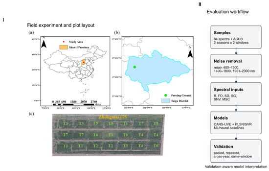
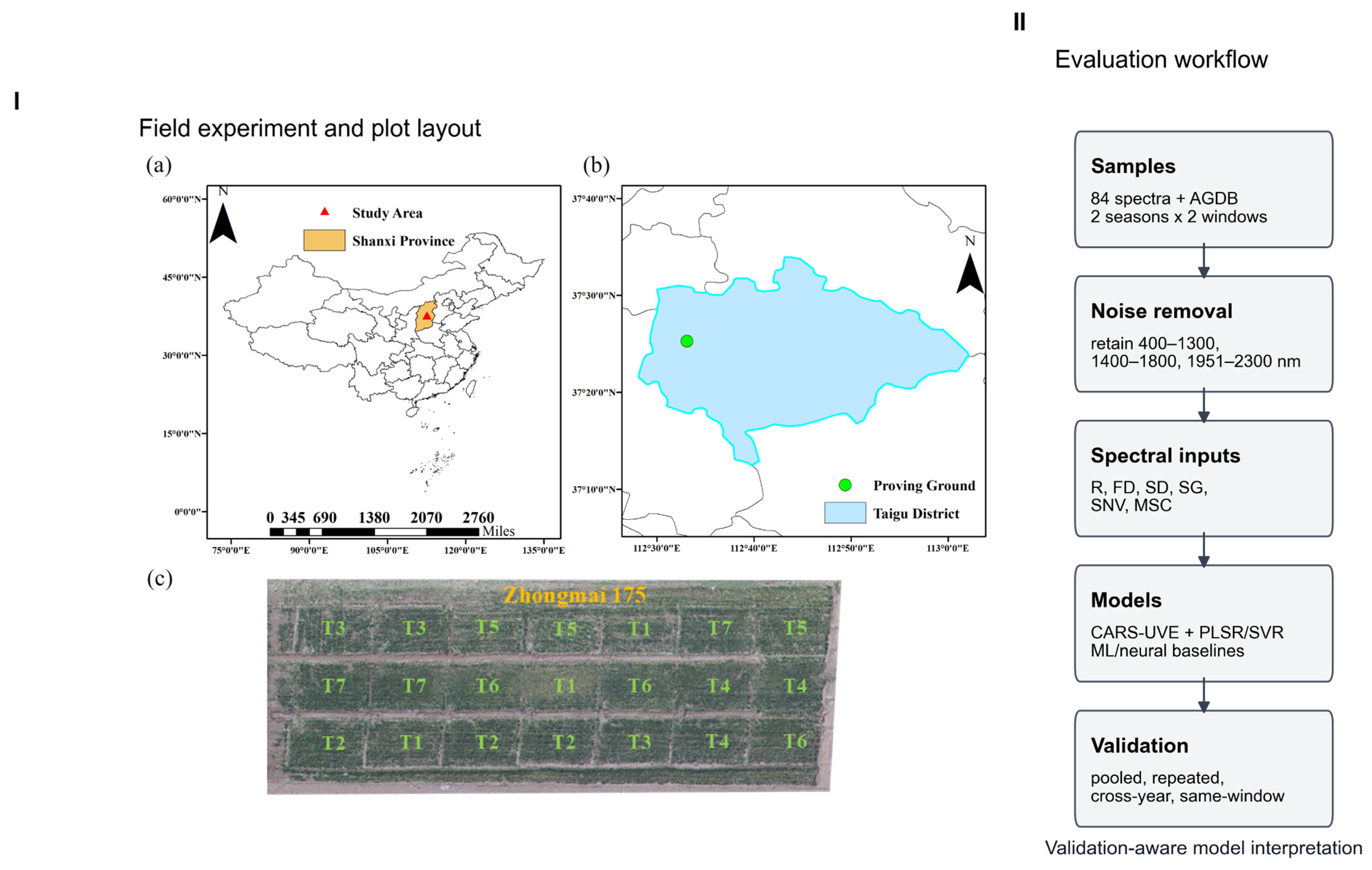
The technical route followed six steps: field sampling and paired AGDB measurement; spectral noise-band removal; construction of six preprocessing matrices; CARS-UVE feature selection performed within each training subset; regression modeling with PLSR, SVR, and additional baselines; and validation by pooled, repeated, full-season transfer, and same-window transfer designs. This workflow is summarized in Figure 1 and was designed to keep preprocessing, feature selection, model fitting, and testing separated.

Figure 1. Field experiment and validation-aware modeling workflow. (I) Field experiment and plot layout; (a) geographic location of Shanxi Province and the study area in China; (b) location of the proving ground within Taigu District; (c) field plot layout and winter wheat cultivar used in the experiment. (II) Modeling workflow separating field sampling, spectral noise-band removal, preprocessing, CARS-UVE selection, regression modeling, and four validation designs.

Four validation designs were used, each answering a different question about the same dataset. First, we used a conventional pooled analysis: a 70/30 random train–test split with random_state = 42. This validation design estimates performance when the calibration and test sets are randomly drawn from the same pooled population. It is useful as a baseline because it matches the common workflow used in many small field spectroscopy studies. However, it does not test whether a model can transfer across seasons or whether it performs well within a narrower phenological window.

Second, because a single split can be overly optimistic in small datasets, especially when model choice is made from the same limited data, we repeated the SG workflow across 20 random train–test partitions [22,24]. SG was chosen because it produced the best pooled single-split result and therefore represented the strongest candidate preprocessing setting. For each repeated split, feature selection and model fitting were re-run rather than reusing the bands selected in the initial pooled split. This design allowed us to estimate not only the variability of prediction accuracy but also the variability of the selected-band subset. The repeated-split analysis therefore functioned as a robustness check on both model performance and feature-selection stability.

Third, we tested full-season cross-year transfer by training on all samples from one season and testing on all samples from the other season, in both directions. This split was used as a temporal analogue of structured validation, which is recommended when observations are not exchangeable across time, space, or biological grouping [23]. The 2021 → 2022 direction tests whether a model calibrated on the first season can predict the second season, whereas the 2022 → 2021 direction tests the reverse transfer. Because each direction uses one full season for training and the other for testing, the test data are not randomly mixed with the training season. This design is more conservative than the pooled split and is more relevant to practical use, where a model developed in one season is often expected to perform in another.

Fourth, we added a stricter same-window cross-year transfer analysis. The modeling matrices did not explicitly store sampling-window labels, but each plot-year identifier appeared twice. The lower-biomass observation within each plot-year pair was treated as the earlier sampling window and the higher-biomass observation as the later window. For the same-window transfer test, models were trained on one season’s earlier-window samples and tested on the other season’s earlier-window samples, and the same procedure was repeated for the later window. This analysis directly tests whether the model captures biomass-specific information within a comparable sampling window rather than benefiting from the broad early-to-late biomass gradient. Because each same-window transfer used only 21 training and 21 testing observations, it was interpreted as a stringent sensitivity analysis rather than as a fully powered benchmark.

Model performance was evaluated with the coefficient of determination (R²), root mean square error (RMSE), and ratio of performance to deviation (RPD). R² was used to quantify the proportion of test-set variance explained by the model. RMSE was used to express prediction error in the native AGDB unit. RPD was used as a scale-normalized indicator of predictive usefulness by comparing the spread of observed values with the residual error. For repeated random splits, we reported the mean, standard deviation, and 95% confidence interval across 20 splits. For transfer tests, bootstrap confidence intervals were calculated from test-set predictions, and paired Wilcoxon signed-rank tests were used to compare absolute errors from models evaluated on the same test samples. Model training time was recorded with Python’s time.perf_counter() and is reported as an implementation-specific computational reference. The analysis environment was Windows 10 64-bit on an Intel64 CPU architecture, using Python 3.11.7, NumPy 1.26.4, pandas 2.1.4, SciPy 1.11.4, scikit-learn 1.2.2, and Matplotlib 3.8.0. These metrics were interpreted jointly. A high R² accompanied by poor transferability, wide uncertainty, long training time, or unstable feature selection was not treated as sufficient evidence for recommending a model.

3. Results

3.1. Pooled Dataset Characteristics

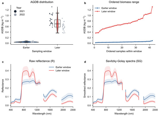
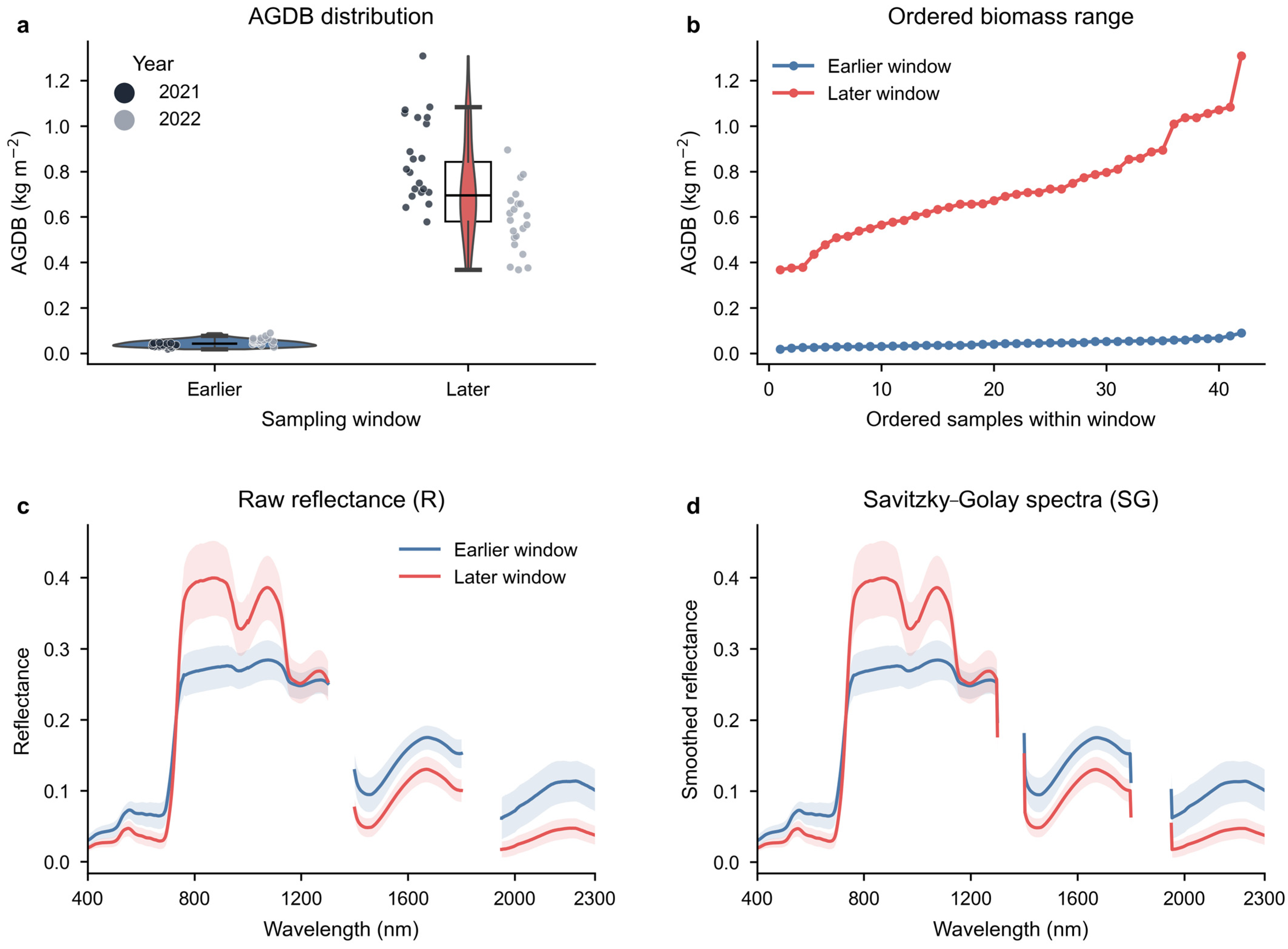
The pooled AGDB dataset spanned a broad range, from 0.0180 to 1.3080 kg m⁻². This range reflects the combination of two seasons, two sampling windows, and multiple nitrogen-management regimes. The inferred earlier window had a much lower biomass than the later window, with mean AGDB values of 0.0436 and 0.7208 kg m⁻², respectively. The seasonal contrast was also clear: the 2021 observations had a mean AGDB of 0.4447 kg m⁻², whereas the 2022 observations had a mean of 0.3197 kg m⁻². Within the later window, the seasonal difference was especially pronounced, with mean AGDB values of 0.8563 kg m⁻² in 2021 and 0.5852 kg m⁻² in 2022. These descriptive statistics indicate that the pooled dataset did not represent a narrow biomass gradient. Instead, it combined very low early-window biomass, substantially higher later-window biomass, and year-to-year differences in crop development.

The canopy spectra showed the expected structure of healthy vegetation, including low reflectance in the visible region, a rise through the red-edge transition, and elevated near-infrared reflectance. The spectral summaries also showed that the early and later sampling windows differed not only in biomass but also in canopy optical expression. This is important because the same spectral contrast that supports accurate pooled prediction can also make the validation task easier. When a training set and test set both contain a mixture of early and late observations, a model may exploit strong differences in canopy structure and pigment absorption associated with phenological development. Therefore, Figure 2 is not presented merely as descriptive background. It defines the data structure that later explains why pooled random-split performance must be interpreted cautiously.

Figure 2. Pooled AGDB distribution and representative canopy spectra. Panels (a,b) show that early- and later-window observations formed a broad biomass gradient. Panels (c,d) show raw reflectance and SG-smoothed reflectance, with clear sampling-window differences in visible, red-edge, and near-infrared regions.

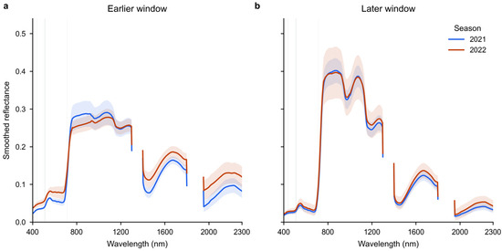
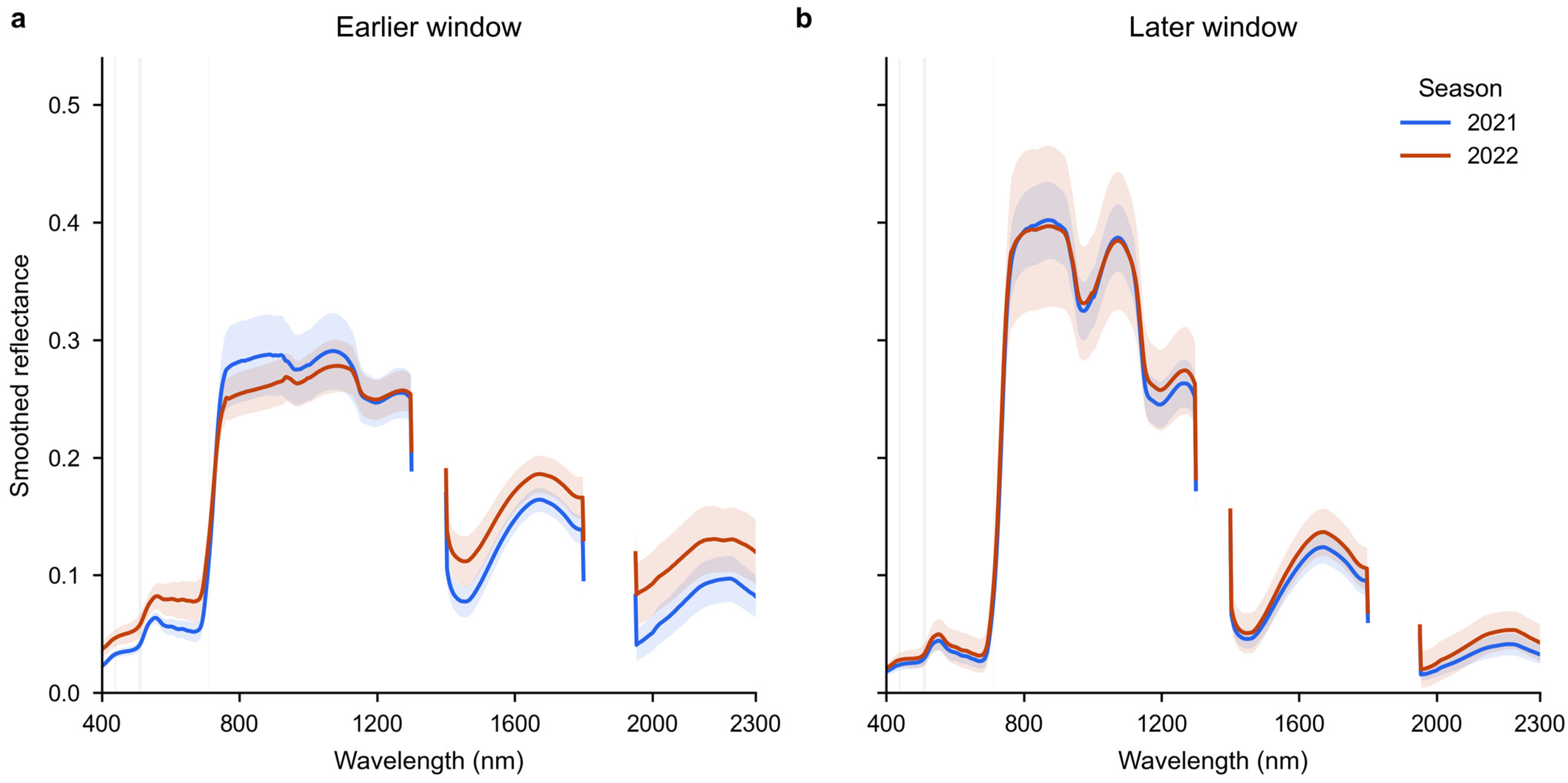
When the SG spectra were summarized separately by year within each sampling window, the two seasons showed clear optical differences. In the earlier window, 2022 had a higher visible reflectance than 2021, whereas 2021 had a slightly higher reflectance across parts of the near-infrared plateau. In the later window, the two years were more similar in the visible and red-edge regions, but 2022 tended to show higher shortwave-infrared reflectance. The shaded regions in Figure 3 mark the recurrent wavelength intervals identified later by repeated band selection. Their location in the blue-green and red-edge portions of the spectrum indicates that selected wavelengths occurred in regions where both year and sampling-window effects were visible. This year-wise spectral contrast helps explain why temporal transfer is a more demanding validation problem than a pooled random split.

Figure 3. Year-specific SG reflectance profiles within the same sampling window. (a) Earlier sampling window, showing 2021 and 2022 SG reflectance profiles and year-to-year differences in the visible and near-infrared (NIR) ranges; (b) later sampling window, showing 2021 and 2022 SG reflectance profiles and year-to-year differences mainly in the shortwave-infrared (SWIR) range. The y-axis is smoothed reflectance; shaded intervals mark recurrent selected wavelength regions.

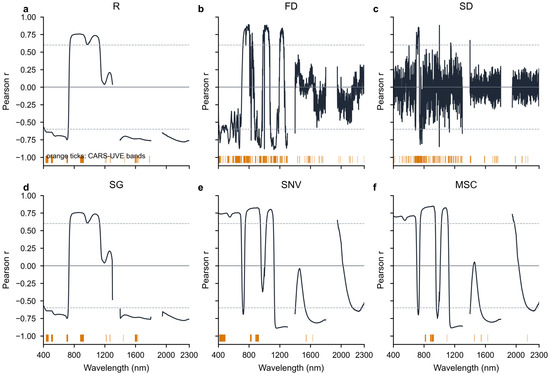
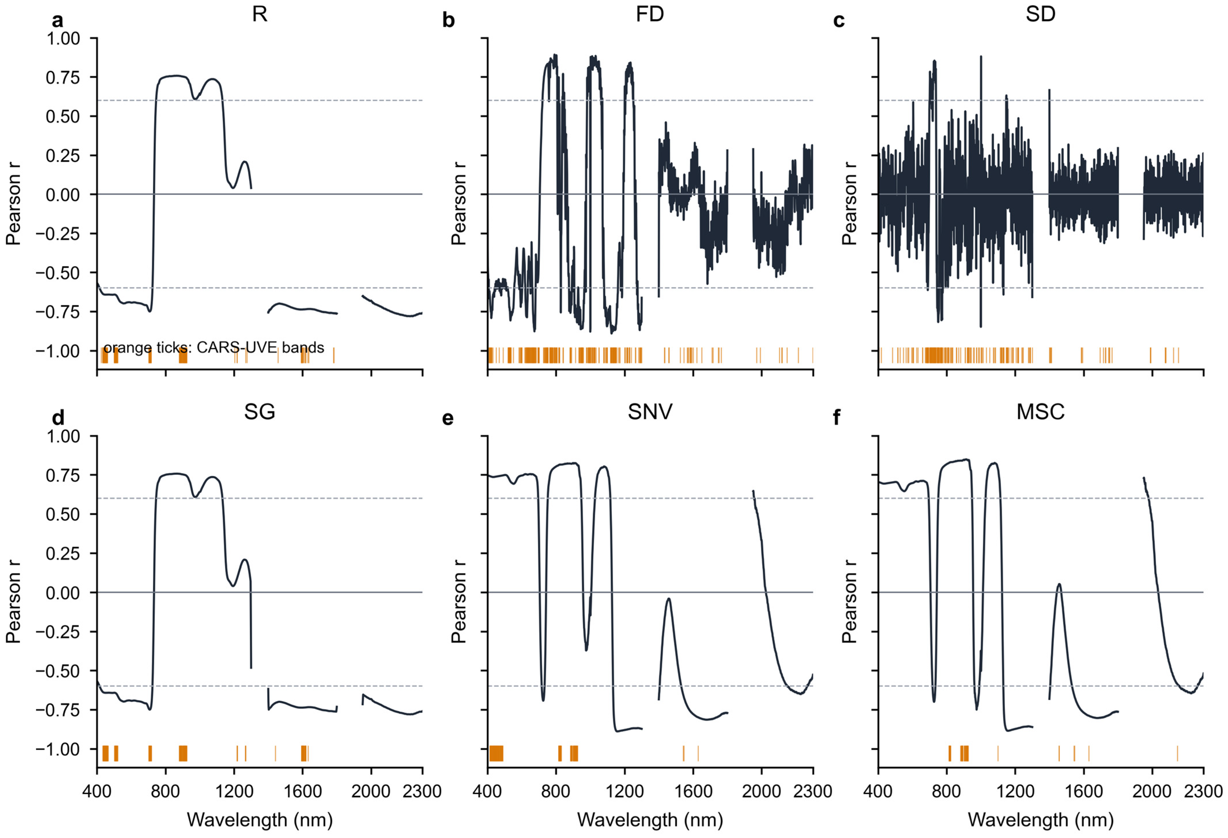
Wavelength-level correlations with AGDB also differed among preprocessing inputs (Figure 4). Some transformations concentrated strong positive or negative associations in the visible and red-edge regions, whereas others distributed correlation structure more broadly across the retained spectral range. The CARS-UVE selected bands tended to occur in regions with a meaningful wavelength-response structure, but the selected locations and density differed strongly among preprocessing inputs. This pattern helps explain why selected-band counts and model performance varied across preprocessing strategies. Because raw and SG profiles are already summarized in Figure 2 and Figure 3, and the full transformed profiles are documented in Supplementary Figure S1, Figure 4 focuses on the correlation structure and selected-band overlays that most directly connect preprocessing to model evidence.

Figure 4. Wavelength-wise AGDB correlations and CARS-UVE selected-band overlays under different spectral inputs. (a) Raw reflectance (R); (b) first-derivative spectra (FD); (c) second-derivative spectra (SD); (d) Savitzky-Golay-smoothed spectra (SG); (e) standard normal variate-transformed spectra (SNV); (f) multiplicative scatter correction-transformed spectra (MSC). In each panel, the black curve shows the Pearson correlation coefficient between AGDB and the corresponding wavelength variable; the solid horizontal line marks r = 0, and the dashed horizontal lines mark the reference levels of r = ±0.6. Orange ticks at the bottom indicate wavelengths selected by CARS-UVE.

3.2. Conventional Pooled Random-Split Evaluation Favored SG-CARS-UVE-SVR

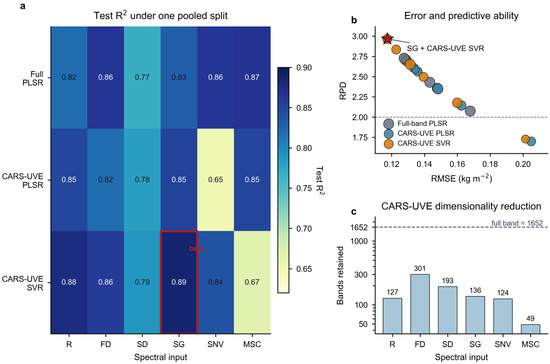
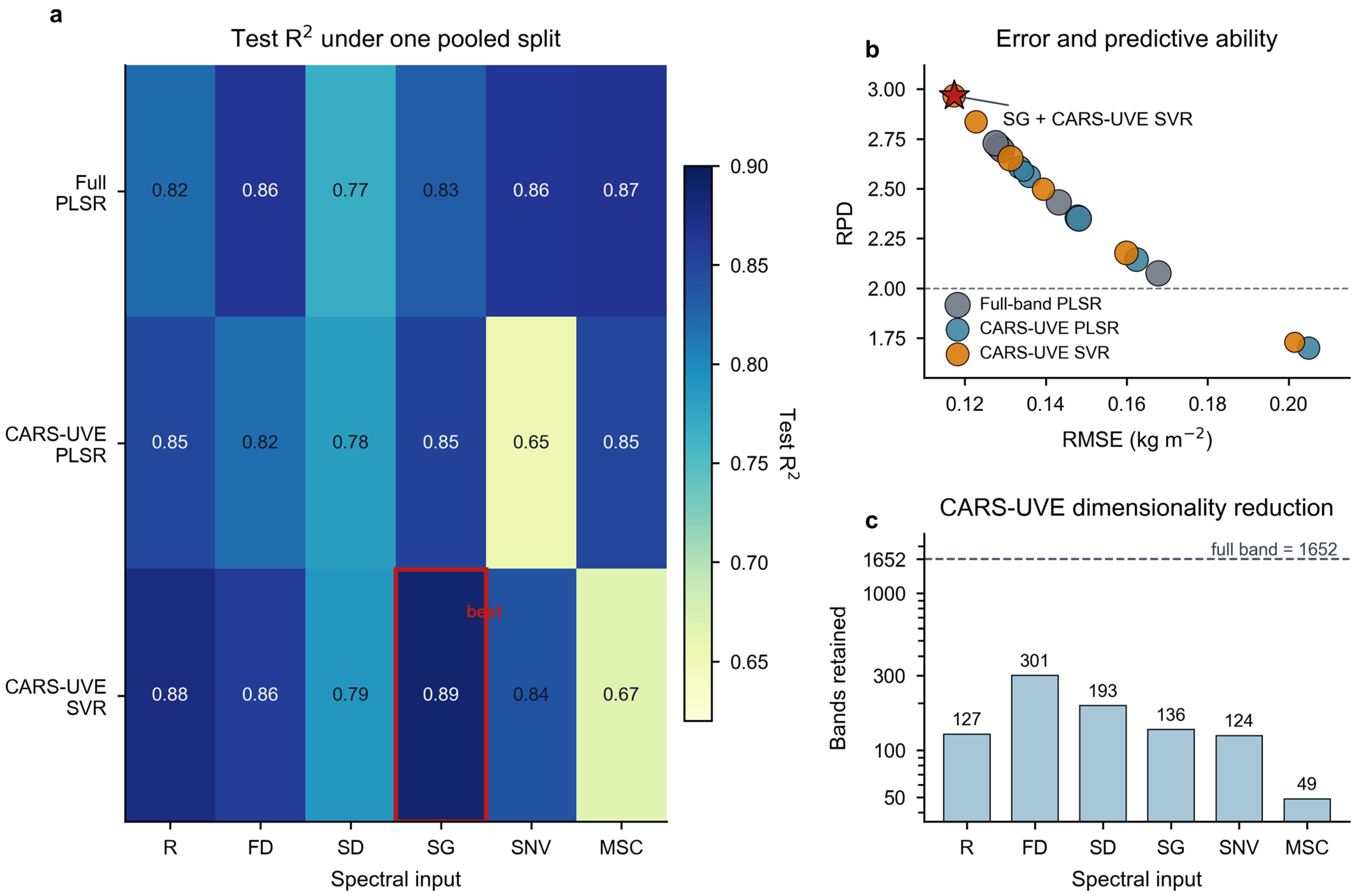
Under the conventional pooled 70/30 random split, preprocessing and feature selection both affected apparent model performance (Table 1 and Figure 5). The best overall result was obtained by SG + CARS-UVE + SVR, with R² = 0.8864, RMSE = 0.1174 kg m⁻², and RPD = 2.9665. This result was visually and numerically attractive because it combined the lowest test error with the highest RPD among all tested combinations. Selected-band PLSR also improved under SG preprocessing and reached R² = 0.8528, indicating that the SG selected-band subset retained substantial biomass information even under a linear latent-variable model. Across preprocessing inputs, the number of selected bands varied substantially, from 49 for MSC to 301 for FD, indicating that preprocessing strongly altered the feature-selection outcome.

Table 1. Performance of six preprocessing inputs under a conventional pooled random split.

Preprocessing Input	Model	Selected Bands	R2	RMSE (kg m−2)	RPD
R	Full-band PLSR	1652	0.8196	0.1479	2.3544
R	CARS-UVE PLSR	127	0.8476	0.1359	2.5615
R	CARS-UVE SVR	127	0.8756	0.1228	2.8354
FD	Full-band PLSR	1652	0.8640	0.1284	2.7112
FD	CARS-UVE PLSR	301	0.8189	0.1482	2.3496
FD	CARS-UVE SVR	301	0.8578	0.1313	2.6519
SD	Full-band PLSR	1652	0.7676	0.1678	2.0745
SD	CARS-UVE PLSR	193	0.7824	0.1624	2.1435
SD	CARS-UVE SVR	193	0.7890	0.1599	2.1770
SG	Full-band PLSR	1652	0.8308	0.1432	2.4307
SG	CARS-UVE PLSR	136	0.8528	0.1336	2.6065
SG	CARS-UVE SVR	136	0.8864	0.1174	2.9665
SNV	Full-band PLSR	1652	0.8623	0.1292	2.6953
SNV	CARS-UVE PLSR	124	0.6536	0.2049	1.6990
SNV	CARS-UVE SVR	124	0.8396	0.1394	2.4971
MSC	Full-band PLSR	1652	0.8656	0.1276	2.7281
MSC	CARS-UVE PLSR	49	0.8506	0.1346	2.5875
MSC	CARS-UVE SVR	49	0.6652	0.2015	1.7281

Figure 5. Conventional pooled single-split comparison of preprocessing and model combinations. (a) Test R² heatmap for six spectral inputs and three modeling workflows; the red box marks the best combination. (b) RMSE–RPD scatter plot, where gray, blue, and orange points represent full-band PLSR, CARS-UVE PLSR, and CARS-UVE SVR, respectively, and the red star indicates SG + CARS-UVE + SVR. (c) Number of wavelengths retained by CARS-UVE for each spectral input; the dashed line indicates the full-band dimensionality.

The pooled single-split ranking suggested three preliminary conclusions. First, the hybrid selection workflow could reduce spectral dimensionality without necessarily degrading accuracy. For example, the SG selected-band models used only 136 bands instead of the full 1652 bands, yet both selected-band PLSR and selected-band SVR outperformed the full-band SG PLSR result. Second, SG produced the most favorable balance between signal preservation and noise suppression for the pooled split, whereas other transformations had mixed effects. The R and FD inputs also performed well with selected-band SVR, but SNV and MSC showed weaker selected-band SVR performance despite reasonable full-band PLSR results. Third, the nonlinear SVR model seemed advantageous when tuned on selected bands, particularly for R and SG spectra. Taken alone, these results would suggest that CARS-UVE reduces dimensionality, SG is a favorable preprocessing method, and SVR provides the strongest pooled prediction.

However, Table 1 also contains early evidence that the single-split conclusion should be treated cautiously. Full-band PLSR performed consistently across several preprocessing inputs, with test R² values above 0.81 for R, FD, SG, SNV, and MSC. The difference between the best selected-band SVR model and several simpler full-band PLSR alternatives was therefore not as large as the single best value alone might suggest. In addition, selected-band performance was not uniformly better than full-band performance. SNV selected-band PLSR dropped to R² = 0.6536, and MSC selected-band SVR dropped to R² = 0.6652. These weaker combinations show that the CARS-UVE cascade was not automatically beneficial across all spectral inputs and regression families. The conventional split therefore provided a useful baseline, but it did not by itself establish that the apparent best model was robust.

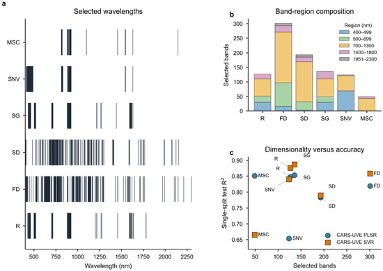
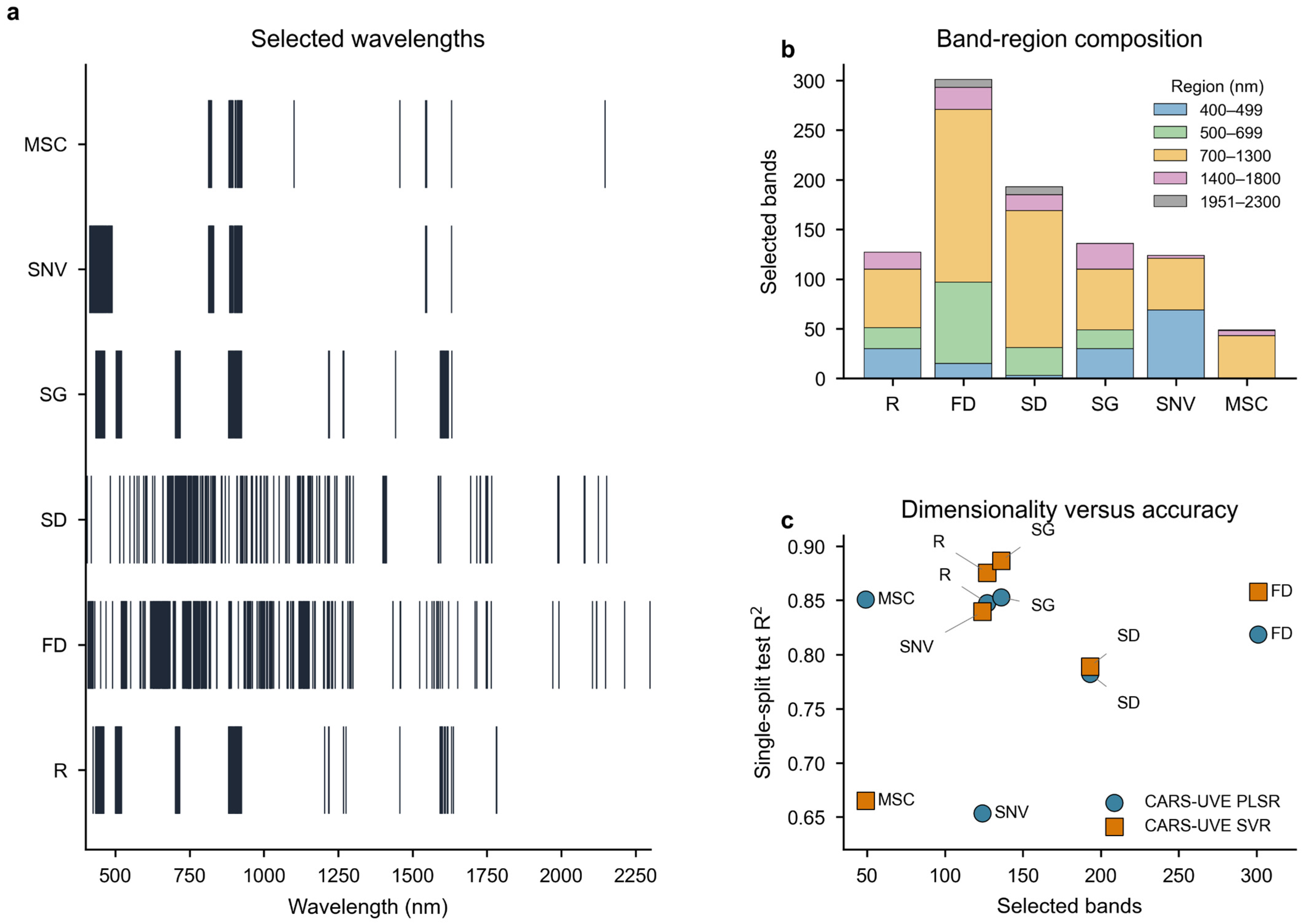
The selected-band architecture from the same pooled split provides an additional view of the conventional result (Figure 6). FD retained the largest selected subset (301 bands), whereas MSC retained the smallest (49 bands). The selected bands were not evenly distributed across the spectrum. Most preprocessing inputs retained many bands in the 700–1300 nm region, while visible-region retention was more prominent for R, SG, and SNV. This pattern indicates that preprocessing changed not only prediction accuracy but also the spectral evidence used by the CARS-UVE cascade.

Figure 6. Single-split CARS-UVE selected-band structure across preprocessing inputs. (a) Selected wavelength distribution; (b) band-region composition; (c) selected-band number versus single-split test R². Selected bands were unevenly distributed and varied strongly among preprocessing inputs.

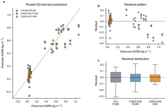
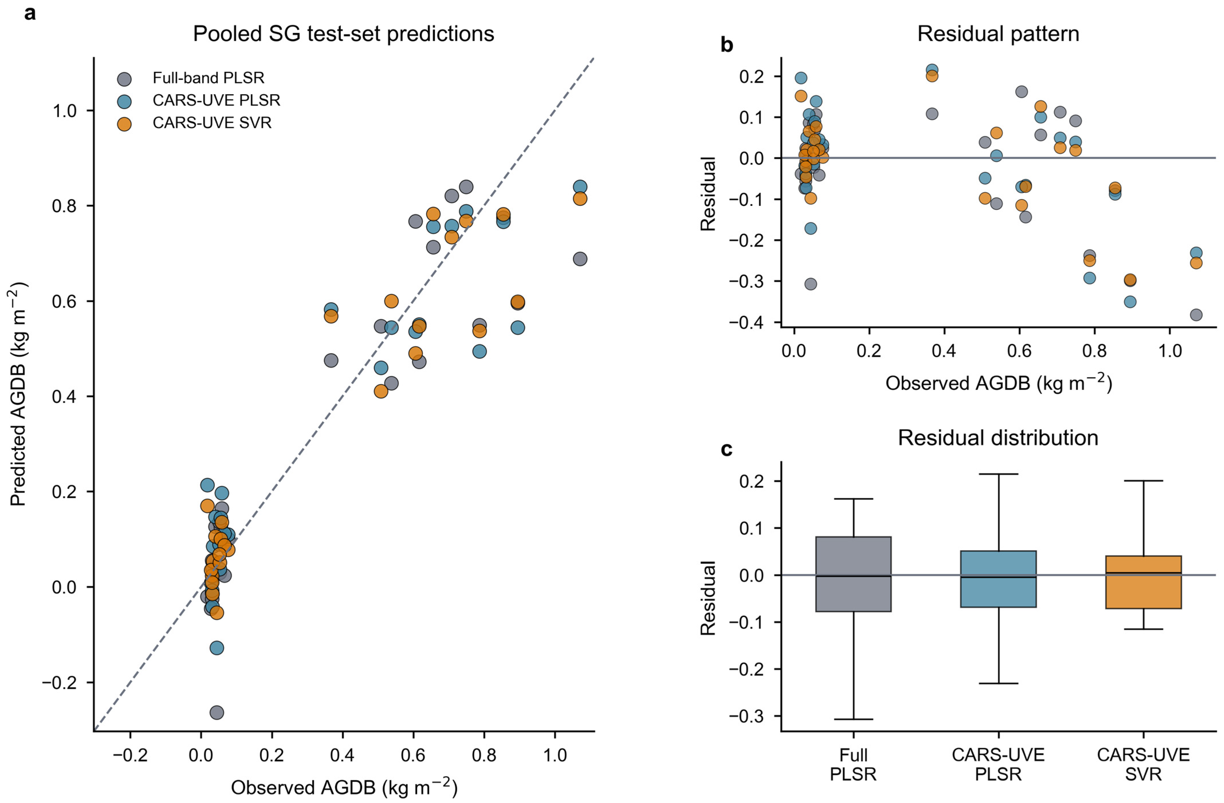
Prediction diagnostics for the SG split confirmed the apparent advantage of CARS-UVE-SVR under the conventional validation view (Figure 7). The selected-band SVR predictions were closer to the 1:1 line and had a narrower residual distribution than the two PLSR alternatives. However, the diagnostic figure also shows why this result should be interpreted as a pooled test-set result rather than a general proof of transferability. The test samples still represent the same pooled population used for random splitting, and the residuals do not challenge year-to-year or within-window generalization.

Figure 7. SG pooled test-set prediction diagnostics for three modeling workflows. (a) Observed versus predicted AGDB; (b) residuals against observed AGDB; (c) residual distributions. Gray, blue, and orange symbols indicate full-band PLSR, CARS-UVE PLSR, and CARS-UVE SVR, respectively.

3.3. Repeated Splitting, Confidence Intervals, and Additional Baselines Quantified Uncertainty

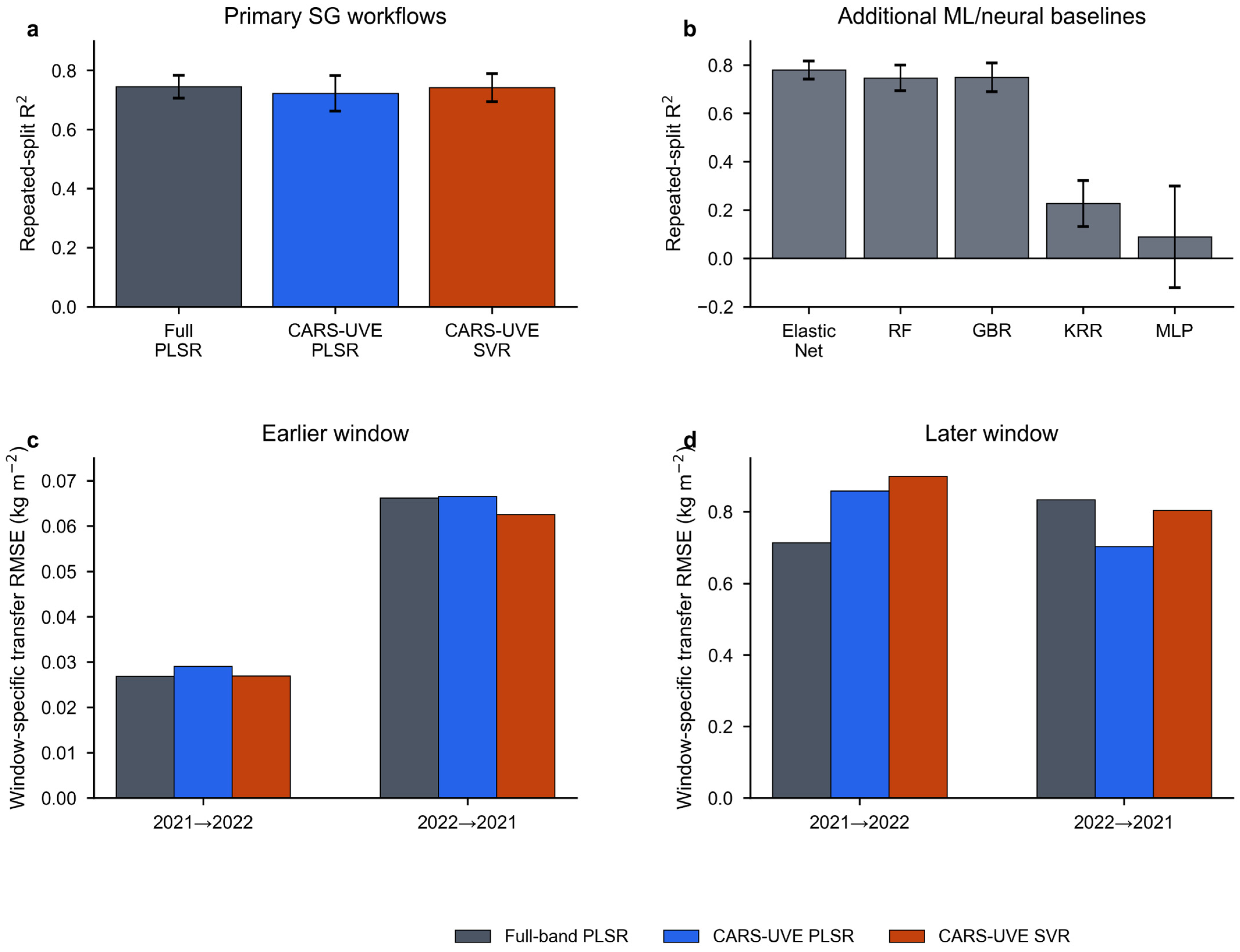
The pooled SG result was not stable when the train–test partition changed. Across 20 random splits, the mean R² of CARS-UVE-SVR was 0.7413, with a 95% confidence interval of 0.6941–0.7885 (Table 2). This interval overlapped strongly with full-band PLSR (0.7448, 0.7058–0.7837) and CARS-UVE-PLSR (0.7223, 0.6625–0.7822). Pairwise Wilcoxon tests based on split-level R² values showed no significant advantage for CARS-UVE-SVR over full-band PLSR (p = 0.5706) or over CARS-UVE-PLSR (p = 0.6215). Thus, the large advantage suggested by the single best split was not maintained under repeated resampling.

Table 2. Repeated-split uncertainty for the primary SG workflows and additional SG-based machine-learning baselines.

Model	Repeated-Split R2 Mean (95% CI)	RMSE Mean (95% CI, kg m−2)	RPD Mean (95% CI)
Full-band PLSR	0.7448 (0.7058–0.7837)	0.1764 (0.1625–0.1903)	2.0630 (1.8888–2.2371)
CARS-UVE PLSR	0.7223 (0.6625–0.7822)	0.1834 (0.1600–0.2067)	2.0506 (1.8209–2.2804)
CARS-UVE SVR	0.7413 (0.6941–0.7885)	0.1780 (0.1574–0.1987)	2.0908 (1.8736–2.3081)
Elastic Net	0.7795 (0.7423–0.8166)	0.1648 (0.1469–0.1827)	2.2895 (2.0711–2.5079)
Random Forest	0.7461 (0.6933–0.7990)	0.1750 (0.1554–0.1946)	2.1708 (1.9421–2.3996)
Gradient Boosting	0.7488 (0.6900–0.8076)	0.1737 (0.1519–0.1955)	2.2068 (1.9588–2.4549)
Kernel Ridge	0.2264 (0.1308–0.3220)	0.3123 (0.2835–0.3412)	1.1860 (1.1182–1.2538)
Exploratory MLP	0.0886 (−0.1221–0.2993)	0.3282 (0.2912–0.3651)	1.1632 (1.0286–1.2977)

The repeated-split distributions also revealed that single-split model ranking could be reversed by sample allocation. The worst split for CARS-UVE PLSR had R² = 0.4705, while the best split reached R² = 0.9059. CARS-UVE SVR ranged from 0.5396 to 0.9063, and full-band PLSR ranged from 0.5526 to 0.8930. Such wide ranges are not surprising for a dataset with only 84 observations, but they are important for interpretation. A researcher reporting only the most favorable split could reasonably conclude that the selected-band nonlinear model was excellent. A researcher seeing the full repeated-split distribution would instead conclude that model performance depends strongly on how the pooled samples are partitioned.

Additional SG-based machine-learning baselines did not overturn this interpretation. Elastic Net produced the highest mean repeated-split R² among the added baselines (0.7795, 95% CI 0.7423–0.8166), followed by gradient boosting (0.7488, 0.6900–0.8076) and random forest (0.7461, 0.6933–0.7990). Kernel ridge regression was weaker (R² = 0.2264), and the exploratory MLP neural baseline was unstable (R² = 0.0886, 95% CI −0.1221–0.2993). These results show that adding more flexible or more modern machine-learning models does not by itself solve the validation problem. The strongest additional baselines were competitive under repeated random splitting, but transfer-oriented validation remained necessary before any model could be recommended for cross-season use.

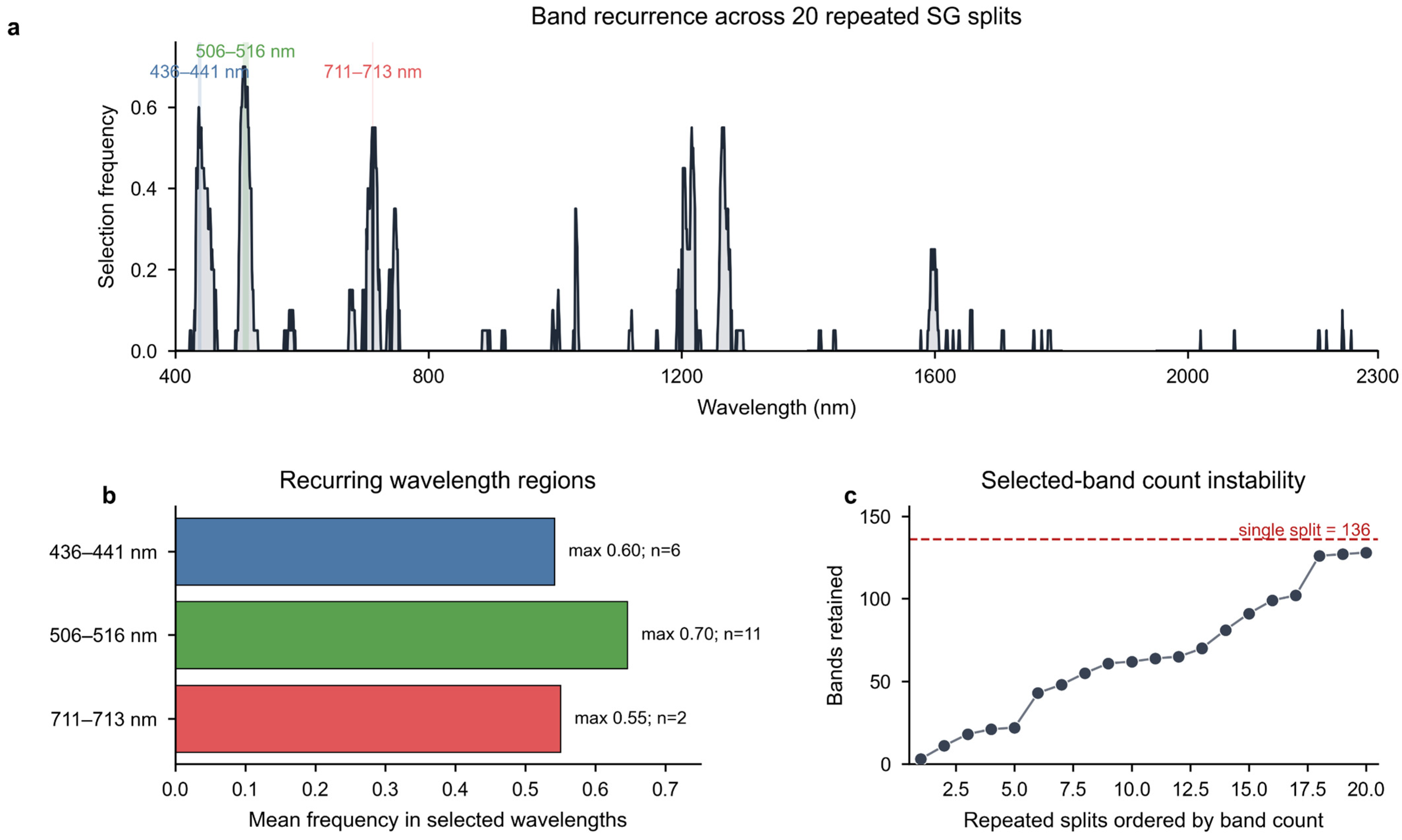
The selected-band count was also unstable. Across the 20 SG-based CARS-UVE runs, the number of retained bands ranged from 3 to 128, with a mean of 64.85 and an SD of 38.84. The lower quartile was 37.75 bands and the upper quartile was 93.00 bands, indicating that the instability was not caused by a single outlying split. This variation means that the dimensionality-reduction step was highly sensitive to the training composition. Even so, the recurrent wavelength frequencies were not random. The most frequently retained bands clustered in the 436–441 nm, 506–516 nm, and 711–713 nm regions, pointing to repeated selection of blue-green and red-edge transition information. Therefore, the repeated analysis weakens the claim of a stable single selected-band set, but it still supports a more cautious claim about recurrent spectral regions.

Training time was short for most baselines on the local workstation. Mean repeated-split fitting time was approximately 0.27 s for Elastic Net, 0.30 s for random forest, 2.09 s for gradient boosting, 0.003 s for kernel ridge regression, and 0.27 s for the exploratory MLP. The CARS-UVE workflows required additional feature-selection time, commonly around one second per transfer fit in the present implementation. These values should be interpreted as implementation-specific computational references, but they show that the main limitation was statistical robustness rather than computational feasibility.

3.4. Cross-Year Transfer Favored PLSR over the Pooled Best SVR Model

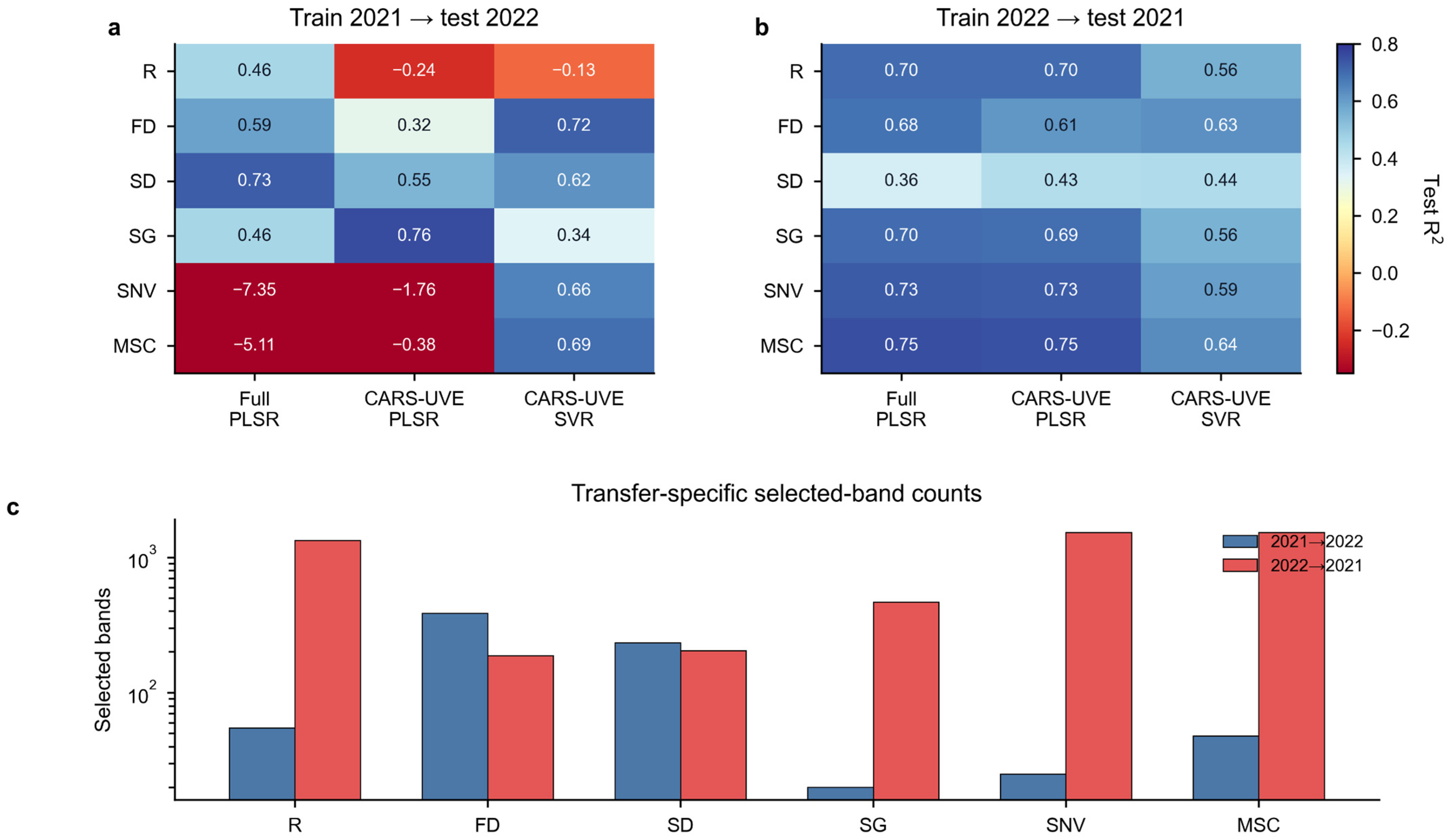
Cross-year transfer produced a different model ranking from the pooled random split. When models were trained on the first season and tested on the second, SG + CARS-UVE + PLSR provided the best SG-based result, with R² = 0.7577, RMSE = 0.1391 kg m⁻², and RPD = 2.0316. The full-band SG PLSR model was substantially weaker in this direction (R² = 0.4606), while the SG selected-band SVR model dropped further to R² = 0.3402. In the reverse direction, SG-based full-band and selected-band PLSR were similar (R² = 0.6973 and 0.6938, respectively), whereas SG selected-band SVR was again weaker (R² = 0.5574). Considering all preprocessing inputs, the best reverse-direction result came from MSC + full-band PLSR, with R² = 0.7506 and RPD = 2.0025. These transfer results suggest that the most transferable configuration was not the pooled best nonlinear model.

The asymmetry between transfer directions is informative. Training on 2021 and testing on 2022 required the model to predict a season with lower later-window biomass and a different AGDB distribution. In that setting, selected-band PLSR on SG spectra performed best among the SG workflows, suggesting that compact linear latent-variable structure was more useful than nonlinear flexibility. Training on 2022 and testing on 2021 required transfer toward a season with higher later-window biomass, where full-band PLSR remained competitive. The selected-band counts also differed strongly between directions, with 20 retained SG bands for 2021 → 2022 and 468 for 2022 → 2021. This contrast reinforces the view that the calibration season affects both the chosen spectral subset and the resulting transfer performance.

SVR performance degraded more strongly under year transfer. The pooled best SG + CARS-UVE + SVR model had achieved R² = 0.8864 in the conventional split, but dropped to R² = 0.3402 when trained on 2021 and tested on 2022, and to R² = 0.5574 in the reverse direction. The same qualitative pattern was observed across several other preprocessing inputs. In contrast, PLSR results were more consistent across directions, even when the best preprocessing input changed from SG to MSC. This indicates that model simplicity and latent-variable regularization may be more beneficial than nonlinear flexibility when extrapolation across seasons is required.

The uncertainty analysis for temporally structured SG predictions supported this interpretation. Bootstrap intervals for transfer-test performance were wide, as expected with 42 test observations per full-season direction and only 21 test observations per same-window direction. Paired Wilcoxon tests on absolute errors showed that CARS-UVE SVR had larger errors than CARS-UVE PLSR in both full-season SG transfer directions (p = 0.0032 for 2021 → 2022 and p = 0.0058 for 2022 → 2021; Supplementary Table S1). These tests reinforce the conclusion that the pooled nonlinear advantage did not provide stable evidence for temporal transfer.

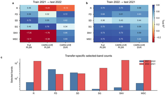
The full cross-year matrix confirmed that the transfer result was not a peculiarity of the SG input alone (Figure 8). Several preprocessing inputs produced moderate transfer performance in one direction but weak or negative performance in another, and the best configuration differed between transfer directions (Figure 8a,b). The heatmap also shows that selected-band counts changed sharply between years for some preprocessing inputs, indicating that temporal transfer affected both prediction accuracy and the spectral subset chosen by CARS-UVE (Figure 8c).

Figure 8. Cross-year transfer performance across all preprocessing inputs. (a) Test R² for models trained in 2021 and tested in 2022; (b) test R² for models trained in 2022 and tested in 2021; (c) transfer-specific selected-band counts.

3.5. Same-Window Cross-Year Transfer Exposed the Phenological-Gradient Effect

The full-season cross-year test was stricter than a pooled random split, but it still trained and tested on both sampling windows. We therefore added same-window cross-year transfer as a more demanding sensitivity analysis. This analysis produced substantially weaker performance than the pooled and full-season transfer results (Figure 9). In the earlier-window 2021 → 2022 direction, RMSE values were small in absolute terms (0.0269–0.0290 kg m⁻²) because the biomass range was narrow, but all R² values were negative (−3.69 to −3.02). In the reverse earlier-window direction, RMSE increased to 0.0626–0.0666 kg m⁻², and R² values became extremely negative because the test-set variance was very small.

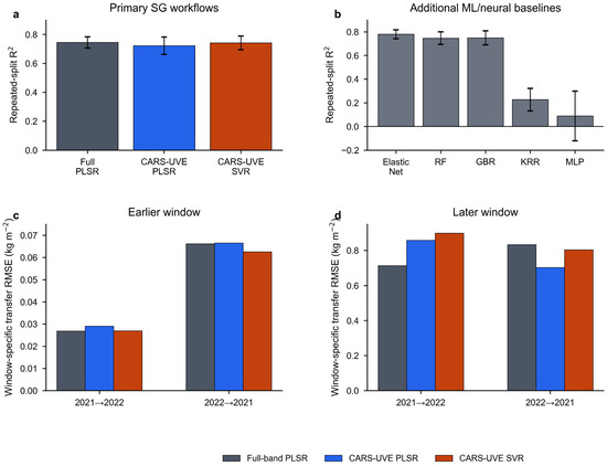
Figure 9. Repeated-split uncertainty, additional ML/neural baselines, and same-window transfer. Panels (a,b) compare repeated-split R² distributions with confidence intervals; panels (c,d) show the stricter same-window cross-year RMSE results.

The later-window same-window transfer was also weak. For 2021 → 2022, full-band PLSR had the lowest RMSE (0.7133 kg m⁻²), whereas CARS-UVE PLSR and CARS-UVE SVR had RMSE values of 0.8581 and 0.8990 kg m⁻², respectively. For 2022 → 2021, selected-band PLSR had the lowest RMSE (0.7027 kg m⁻²), but the corresponding R² remained negative. These results show that none of the primary SG workflows provided reliable same-window year-to-year transfer.

This stricter test clarifies why the pooled split appeared strong. When early and late seasonal samples are mixed, models can exploit large differences in canopy structure, pigment absorption, red-edge position, and biomass that co-vary with phenological state. Same-window transfer removes much of that broad gradient and asks whether the model can predict biomass differences within a comparable sampling window across years. The failure of this test indicates that the strong pooled result should be interpreted as broad seasonal biomass discrimination rather than stable window-invariant biomass inversion.

3.6. Spectral Regions Associated with Robust Selection

The spectral interpretation also changed when robustness, rather than peak accuracy, was emphasized. In the best pooled SG split, informative bands extended across the visible, red-edge, near-infrared, and shortwave-infrared regions (Figure 10). However, under repeated splitting, the most persistent selections were concentrated in the blue-green (436–441 nm, 506–516 nm) and red-edge onset (711–713 nm) regions. Within the 506–516 nm interval, several wavelengths were retained in more than half of the 20 splits, with frequencies reaching 0.70 at 507–510 nm. The 436–441 nm interval also showed repeated retention, with frequencies from 0.50 to 0.60. The red-edge onset was represented by repeated selection at 711 and 713 nm, each with a frequency of 0.55.

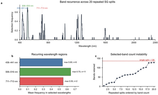
Figure 10. Recurrent selected wavelengths under repeated SG splits. (a) Wavelength-wise selection frequency; (b) summary of recurrent wavelength regions; (c) selected-band count across repeated train–test partitions.

These wavelengths are consistent with variations in pigment absorption, canopy scattering, and structural transitions that co-vary with crop development. Shortwave-infrared bands were important in some pooled fits, but they were less consistently retained across repeated splits. This does not mean that shortwave-infrared information is irrelevant to biomass. Rather, it indicates that, in this small dataset and under repeated random partitioning, visible and red-edge onset regions were more reproducible than individual shortwave-infrared wavelengths. The robust interpretation is therefore regional rather than single-band specific: the workflow repeatedly returned to blue-green and red-edge information, but did not identify one immutable wavelength signature.

4. Discussion

4.1. Why the Pooled Single-Split Result Was Too Optimistic

A pooled random-split result provides a useful baseline, but it is insufficient as the sole evidence for model quality in this dataset. The pooled dataset combined two seasons and two sampling windows, generating a wide AGDB range and large canopy differences. Under those conditions, a single train–test split can reward models that separate broad seasonal states rather than models that recover stable within-window biomass relationships. The strong decline in performance after repeated splitting and same-window cross-year transfer supports that interpretation and is consistent with broader warnings that limited-sample validation can underestimate prediction error when tuning, selection, and testing are weakly separated [22,23,24].

This point matters because small field spectroscopy studies often report one favorable split and then discuss the best model as if it were inherently robust. In the present dataset, that approach would have favored SG + CARS-UVE + SVR. Yet once transfer-oriented validation was added, the nonlinear advantage largely disappeared. The main methodological lesson is that pooled interpolation and temporal transfer are different evaluation problems. A pooled random split can still be informative when the intended use case is interpolation within a similar pooled population. It becomes insufficient, however, when the intended claim involves seasonal transfer, operational monitoring, or biological stability of selected wavelengths. The validation design must match the claim being made.

The observed optimism also has a biological component. Winter wheat canopy spectra change strongly as biomass accumulates, leaves expand, stems develop, and canopy closure increases. These changes affect visible absorption, red-edge slope, near-infrared scattering, and shortwave-infrared response. A model trained on pooled early and later observations can therefore learn a strong composite gradient that is partly biomass and partly phenological state. This does not make the model useless, but it changes the interpretation. The model may be effective for ranking samples across a broad growth gradient, while still being weak for distinguishing smaller biomass differences among samples within the same window. The same-window transfer results support exactly that distinction.

4.2. When Hybrid Band Selection Helped, and When It Did Not

The CARS-UVE cascade remained useful, but its benefit was conditional. Under the pooled split, it reduced dimensionality and improved the best SG and R models. Under cross-year transfer, selected-band PLSR produced the strongest 2021 → 2022 result. These findings support the practical value of hybrid selection for compacting noisy field spectra, a problem widely recognized in chemometric and near-infrared modeling [16,17,18]. However, the repeated-split analysis also showed strong instability in the number of retained bands. The selector could return very small or much larger subsets depending on sample assignment. Therefore, the benefit of hybrid selection should be described as conditional rather than universal.

This conditional benefit also clarifies the difference between PLSR and SVR. The instability observed here is consistent with broader concerns about feature-selection reproducibility in small, high-dimensional datasets [19]. SVR exploited the pooled interpolation problem effectively, but its performance degraded more strongly under year transfer. PLSR, especially in selected-band form, was less spectacular in the best random split but more defensible when extrapolation was required. For practical agronomic sensing, that trade-off favors models that are slightly less accurate in the easiest validation scenario but more stable when the data context changes.

The comparison should not be reduced to a simple claim that linear models are always better than nonlinear models. Rather, the results show that the advantage of nonlinear regression depends on the structure and amount of calibration data. With only 84 observations and strong covariance among wavelengths, SVR may fit the pooled calibration structure well but still fails to extrapolate across seasonal shifts. PLSR imposes a stronger latent-variable structure and is therefore less flexible, but that constraint can be helpful when the test distribution differs from the training distribution. The additional baselines support the same caution. Elastic Net, random forest, and gradient boosting were competitive under repeated random splitting, whereas kernel ridge regression and the exploratory MLP were unstable or weak. Thus, the issue is not whether a more complex machine-learning family can obtain a favorable pooled score; the issue is whether that score survives transfer-oriented validation. In this dataset, the more conservative selected-band or regularized linear interpretations remain more defensible than the peak single-split SVR result.

4.3. Biological Meaning of the Recurrent Spectral Regions

The repeated appearance of blue-green and red-edge bands is consistent with known optical responses of crop canopies. Visible bands near the green peak respond to pigment concentration and leaf optical properties, whereas the red-edge transition is linked to changes in chlorophyll abundance, leaf area, canopy scattering, and biomass-related structural variation [4,27,28,29,30,31]. In the present analysis, these regions were more consistently retained than individual shortwave-infrared bands when the workflow was perturbed across repeated splits. This suggests that they contain more stable cross-sample information for pooled biomass discrimination in the current dataset.

At the same time, the variability of selected subsets cautions against over-interpreting single-band mechanisms. The evidence here is stronger for regional importance than for precise physiological attribution of every wavelength. That is especially true in a small field experiment where spectral selection can be sensitive to the training subset. For example, the repeated selection of bands near 506–516 nm is compatible with pigment-related reflectance variation, and the recurrence near 711–713 nm is compatible with red-edge transition information. However, the analysis does not isolate chlorophyll concentration, leaf area, water content, or canopy structure as separate causal variables. These properties co-vary during crop development. Therefore, the safest interpretation is that the recurrent regions identify stable optical correlates of the pooled biomass gradient, not that each wavelength is a unique physiological marker.

This distinction also affects how the results should be used in future studies. The recurring regions can guide reduced-band sensor design or future hypothesis generation, but they should not be transferred uncritically to another site or season without validation. A compact multispectral configuration derived from these regions might perform well for broad biomass gradients, yet still require local calibration for same-window estimation. Future experiments that measure chlorophyll, leaf area index, canopy water status, and biomass simultaneously would be needed to separate these mechanisms more directly.

4.4. Implications for Winter Wheat Field Spectroscopy Studies

Two practical implications follow. First, model ranking in winter wheat biomass studies should not be based only on pooled random-split performance. Transfer-oriented tests are needed whenever the goal is to support use across seasons or management conditions. A single pooled split may be adequate for preliminary algorithm screening, but it should not be the final basis for recommending an operational model. At minimum, repeated random splits should be used to show whether the apparent ranking is stable. When multi-year data are available, year-to-year transfer provides a more direct test of whether the model can withstand seasonal shifts in canopy development and biomass distribution.

Second, field spectroscopy datasets that span strong phenological contrasts can still be useful, but the resulting models may function primarily as seasonal biomass discriminators rather than window-invariant biomass inversions. Those two use cases are not equivalent and should not be discussed interchangeably. If the intended application is to separate low-biomass and high-biomass crop states across a growing season, a pooled model may be valuable. If the intended application is to estimate biomass within a single sampling window for nitrogen management, irrigation scheduling, or a local treatment comparison, then same-window validation is essential. The present results suggest that the second task is substantially more difficult.

The results also suggest that future reports should distinguish four levels of evidence. The first level is algorithm screening, where many preprocessing and model combinations are compared under a common split. This level is useful for identifying candidate workflows but is not sufficient for model recommendation. The second level is robustness assessment, where repeated splits are used to quantify how sensitive the ranking is to training-set composition. The third level is full-season transfer assessment, where the model is tested across years, sites, cultivars, or management regimes. The fourth level is same-window transfer, which asks whether a model can predict biomass differences after the broad phenological gradient has been restricted. A study that claims operational relevance should include at least the second level and preferably a structured transfer test. Without that distinction, the best-performing model in a table can easily become overstated as a general solution.

For future work, a stronger design would combine multi-site sampling, explicit sampling-window labels in the modeling matrices, and external validation at the level of season or site. Sampling-window-aware or hierarchical modeling may also help separate phenology-driven variation from biomass-specific variation. Another useful extension would be to compare models trained separately within sampling windows with models that include sampling windows as an explicit covariate. This would help determine whether poor within-window performance reflects insufficient sample size, weak spectral sensitivity within each window, or the absence of sampling-window-aware modeling. Additional agronomic measurements, such as leaf area index, chlorophyll content, canopy water status, and final yield, would also make it possible to test whether selected spectral regions are responding directly to biomass or indirectly to correlated canopy traits. Until then, simpler transfer-oriented models provide a safer basis for agronomic interpretation.

4.5. Limitations

This study has four main limitations. First, the experiment was conducted at a single location. The results therefore reflect the soil, climate, cultivar, and management context of the Mengjiazhuang Experimental Base, and they should not be treated as evidence of direct geographic transfer. Second, the sample size remained modest for nonlinear hyperspectral modeling. Although 84 plot-window observations are common in destructive field spectroscopy studies, this number is small relative to the 1652 retained wavelength variables. Third, the strongest result came from pooled samples that spanned broad seasonal contrasts, which inflated apparent interpolation performance. Fourth, the same-window transfer analysis relied on data-derived early and late window labels rather than an explicitly labeled stage column inside the modeling matrices.

These limitations do not invalidate the analysis, but they restrict the scope of inference. This study should therefore be read as a robustness-focused evaluation of a two-season field spectroscopy dataset, not as a final operational biomass monitoring solution. Its main contribution is methodological: it shows that validation design can change the model ranking and the strength of the resulting agronomic interpretation. The study does not claim that the selected-band PLSR workflow is universally optimal for winter wheat, nor does it claim that SVR is unsuitable for all hyperspectral biomass applications. Instead, it demonstrates that a model selected from peak single-split accuracy can be less defensible than a simpler model when repeated and temporal validation are considered.

Several additional constraints should be considered when using the present results. The sampling-window labels used for sensitivity analysis were inferred from paired biomass order, not imported as recorded field metadata. The inference is reasonable for this dataset because the two observations within each plot-year showed a clear biomass progression, but future experiments should store sampling stage, date, thermal time, and phenological score explicitly. The validation design also remains limited by the available sample size. Repeated random splitting reveals instability, but it cannot fully replace independent external validation. Finally, the current analysis evaluates reflectance spectra and biomass only. It does not model soil background, illumination variation, canopy height, disease status, water stress, or independent leaf biochemical traits as separate factors. These unmeasured variables may partly explain why a model that performs well in pooled interpolation becomes less reliable when the season or sampling window changes.

5. Conclusions

This study shows that model ranking for winter wheat AGDB estimation depends strongly on validation design. A conventional pooled random split suggested that SG + CARS-UVE + SVR was the best model (R² = 0.8864, RMSE = 0.1174 kg m⁻², RPD = 2.9665). However, repeated splitting showed overlapping confidence intervals among the primary SG workflows, and full-season cross-year transfer favored simpler PLSR-based interpretations rather than the pooled best SVR model. The stricter same-window transfer analysis further showed that pooled accuracy was strongly supported by broad phenological biomass contrasts and did not translate into reliable window-invariant biomass inversion.

The main contribution is therefore a validation-aware evaluation of a common hyperspectral biomass workflow, not a new universal algorithm. CARS-UVE selection can reduce spectral dimensionality and support accurate pooled prediction, but its selected wavelengths and performance depend on sample allocation. The recurrent regions near 436–441 nm, 506–516 nm, and 711–713 nm provide useful optical clues, but they should be interpreted as regional correlates of canopy development and biomass rather than exact mechanistic wavelengths. For small field hyperspectral datasets, repeated splitting, confidence intervals, and transfer-oriented validation should be treated as routine requirements before recommending a model for cross-season crop monitoring.

References

- He, Z.H.; Xia, X.C.; Chen, X.M.; Zhuang, Q.S. Progress of wheat breeding in China and the future perspective. Acta Agron. Sin. 2011, 37, 202–215. [Google Scholar] [CrossRef] [Scilit]
- Filella, I.; Serrano, L.; Serra, J.; Peñuelas, J. Evaluating wheat nitrogen status with canopy reflectance indices and discriminant analysis. Crop Sci. 1995, 35, 1400–1405. [Google Scholar] [CrossRef] [Scilit]
- Serrano, L.; Filella, I.; Peñuelas, J. Remote sensing of biomass and yield of winter wheat under different nitrogen supplies. Crop Sci. 2000, 40, 723–731. [Google Scholar] [CrossRef] [Scilit]
- Hansen, P.M.; Schjoerring, J.K. Reflectance measurement of canopy biomass and nitrogen status in wheat crops using normalized difference vegetation indices and partial least squares regression. Remote Sens. Environ. 2003, 86, 542–553. [Google Scholar] [CrossRef] [Scilit]
- Mulla, D.J. Twenty five years of remote sensing in precision agriculture: Key advances and remaining knowledge gaps. Biosyst. Eng. 2013, 114, 358–371. [Google Scholar] [CrossRef] [Scilit]
- Baret, F.; Guyot, G. Potentials and limits of vegetation indices for LAI and APAR assessment. Remote Sens. Environ. 1991, 35, 161–173. [Google Scholar] [CrossRef] [Scilit]
- Thenkabail, P.S.; Smith, R.B.; De Pauw, E. Hyperspectral vegetation indices and their relationships with agricultural crop characteristics. Remote Sens. Environ. 2000, 71, 158–182. [Google Scholar] [CrossRef] [Scilit]
- Haboudane, D.; Miller, J.R.; Pattey, E.; Zarco-Tejada, P.J.; Strachan, I.B. Hyperspectral vegetation indices and novel algorithms for predicting green LAI of crop canopies: Modeling and validation in the context of precision agriculture. Remote Sens. Environ. 2004, 90, 337–352. [Google Scholar] [CrossRef] [Scilit]
- Mutanga, O.; Skidmore, A.K. Narrow band vegetation indices overcome the saturation problem in biomass estimation. Int. J. Remote Sens. 2004, 25, 3999–4014. [Google Scholar] [CrossRef] [Scilit]
- Yousfi, S.; Kellas, N.; Saidi, L.; Benlakehal, Z.; Chaou, L.; Siad, D.; Gracia, A. Comparative performance of remote sensing methods in assessing wheat performance under Mediterranean conditions. Agric. Water Manag. 2016, 164, 137–147. [Google Scholar] [CrossRef] [Scilit]
- Yang, C.; Xu, J.; Feng, M.; Bai, J.; Sun, H.; Song, L.; Zhang, M. Evaluation of hyperspectral monitoring model for aboveground dry biomass of winter wheat by using multiple factors. Agronomy 2023, 13, 983. [Google Scholar] [CrossRef] [Scilit]
- Savitzky, A.; Golay, M.J.E. Smoothing and differentiation of data by simplified least squares procedures. Anal. Chem. 1964, 36, 1627–1639. [Google Scholar] [CrossRef] [Scilit]
- Geladi, P.; MacDougall, D.; Martens, H. Linearization and scatter-correction for near-infrared reflectance spectra of meat. Appl. Spectrosc. 1985, 39, 491–500. [Google Scholar] [CrossRef] [Scilit]
- Barnes, R.J.; Dhanoa, M.S.; Lister, S.J. Standard normal variate transformation and de-trending of near-infrared diffuse reflectance spectra. Appl. Spectrosc. 1989, 43, 772–777. [Google Scholar] [CrossRef] [Scilit]
- Tsai, F.; Philpot, W. Derivative analysis of hyperspectral data. Remote Sens. Environ. 1998, 66, 41–51. [Google Scholar] [CrossRef] [Scilit]
- Rinnan, Å.; van den Berg, F.; Engelsen, S.B. Review of the most common pre-processing techniques for near-infrared spectra. TrAC Trends Anal. Chem. 2009, 28, 1201–1222. [Google Scholar] [CrossRef] [Scilit]
- Mehmood, T.; Liland, K.H.; Snipen, L.; Sæbø, S. A review of variable selection methods in partial least squares regression. Chemom. Intell. Lab. Syst. 2012, 118, 62–69. [Google Scholar] [CrossRef] [Scilit]
- Yun, Y.H.; Li, H.D.; Deng, B.C.; Cao, D.S. An overview of variable selection methods in multivariate analysis of near-infrared spectra. TrAC Trends Anal. Chem. 2019, 113, 102–115. [Google Scholar] [CrossRef] [Scilit]
- Khaire, U.M.; Dhanalakshmi, R. Stability of feature selection algorithm: A review. J. King Saud Univ.-Comput. Inf. Sci. 2022, 34, 1060–1073. [Google Scholar] [CrossRef] [Scilit]
- Centner, V.; Massart, D.L.; de Noord, O.E.; de Jong, S.; Vandeginste, B.M.; Sterna, C. Elimination of uninformative variables for multivariate calibration. Anal. Chem. 1996, 68, 3851–3858. [Google Scholar] [CrossRef] [Scilit]
- Li, H.; Liang, Y.; Xu, Q.; Cao, D. Key wavelengths screening using competitive adaptive reweighted sampling method for multivariate calibration. Anal. Chim. Acta 2009, 648, 77–84. [Google Scholar] [CrossRef] [Scilit]
- Varma, S.; Simon, R. Bias in error estimation when using cross-validation for model selection. BMC Bioinform. 2006, 7, 91. [Google Scholar] [CrossRef] [Scilit]
- Roberts, D.R.; Bahn, V.; Ciuti, S.; Boyce, M.S.; Elith, J.; Guillera-Arroita, G.; Hauenstein, S.; Lahoz-Monfort, J.J.; Schröder, B.; Thuiller, W.; et al. Cross-validation strategies for data with temporal, spatial, hierarchical, or phylogenetic structure. Ecography 2017, 40, 913–929. [Google Scholar] [CrossRef] [Scilit]
- Vabalas, A.; Gowen, E.; Poliakoff, E.; Casson, A.J. Machine learning algorithm validation with a limited sample size. PLoS ONE 2019, 14, e0224365. [Google Scholar] [CrossRef] [Scilit]
- Wold, S.; Sjöström, M.; Eriksson, L. PLS-regression: A basic tool of chemometrics. Chemom. Intell. Lab. Syst. 2001, 58, 109–130. [Google Scholar] [CrossRef] [Scilit]
- Cortes, C.; Vapnik, V. Support-vector networks. Mach. Learn. 1995, 20, 273–297. [Google Scholar] [CrossRef] [Scilit]
- Blackburn, G.A. Quantifying chlorophylls and carotenoids at leaf and canopy scales: An evaluation of some hyperspectral approaches. Remote Sens. Environ. 1998, 66, 273–285. [Google Scholar] [CrossRef] [Scilit]
- Daughtry, C.S.T.; Walthall, C.L.; Kim, M.S.; de Colstoun, E.B.; McMurtrey, J.E. Estimating corn leaf chlorophyll concentration from leaf and canopy reflectance. Remote Sens. Environ. 2000, 74, 229–239. [Google Scholar] [CrossRef] [Scilit]
- Gitelson, A.A.; Gritz, Y.; Merzlyak, M.N. Relationships between leaf chlorophyll content and spectral reflectance and algorithms for non-destructive chlorophyll assessment in higher plant leaves. J. Plant Physiol. 2003, 160, 271–282. [Google Scholar] [CrossRef] [Scilit]
- Cho, M.A.; Skidmore, A.K. A new technique for extracting the red edge position from hyperspectral data: The linear extrapolation method. Remote Sens. Environ. 2006, 101, 181–193. [Google Scholar] [CrossRef] [Scilit]
- Delegido, J.; Verrelst, J.; Alonso, L.; Moreno, J. Evaluation of Sentinel-2 red-edge bands for empirical estimation of green LAI and chlorophyll content. Sensors 2011, 11, 7063–7081. [Google Scholar] [CrossRef] [Scilit]
Disclaimer/Publisher’s Note: The statements, opinions and data contained in all publications are solely those of the individual author(s) and contributor(s) and not of MDPI and/or the editor(s). MDPI and/or the editor(s) disclaim responsibility for any injury to people or property resulting from any ideas, methods, instructions or products referred to in the content. |
© 2026 by the authors. Licensee MDPI, Basel, Switzerland. This article is an open access article distributed under the terms and conditions of the Creative Commons Attribution (CC BY) license.