


Highlights
What are the main findings?
- Categorical forest maps discard on average 46.9% of compositional information per pixel in Lualaba Province.
- A Multi-Output Neural Network (MONN) enables continuous, spatially explicit mapping of forest compositional gradients across three forest types.
What are the implications of the main findings?
- Quantifying categorical information loss provides a diagnostic framework for assessing the reliability of forest inventory and carbon stock estimates.
- Accounting for subpixel compositional mixing improves the accuracy of forest assessment in heterogeneous tropical landscapes.
Abstract
Forests of Lualaba Province (DR Congo) form a compositionally complex mosaic of dry dense forest, gallery forest, and Miombo woodland. Yet, categorical land-cover maps impose discrete boundaries on these inherently continuous vegetation gradients, systematically discarding subpixel compositional information critical for forest monitoring and carbon accounting. The magnitude of this information loss at the landscape scale, however, remains largely unquantified. In this study, we train a Multi-Output Neural Network (MONN) using Sentinel-2 spectral and textural predictors (2025) to estimate the proportional cover of three forest types across the province. Model performance is benchmarked against a normalised Random Forest (RF) using spatial block cross-validation. Categorical information loss is quantified pixel-wise using two complementary metrics, dominant class proportion and Shannon compositional entropy, alongside a derived interpretive quantity, categorical information loss. The MONN slightly outperformed RF (R2 = 0.648 vs. 0.630; RMSE = 0.224 vs. 0.229), yet the results reveal a fundamentally heterogeneous landscape structure. The mean dominant-class proportion was only 56.2%, indicating that categorical maps discard, on average, 43.8% of compositional information per pixel. Only 7.9% of forested pixels exceeded the 75% dominance threshold, while Shannon entropy reached 74.1% of its theoretical maximum, indicating that forest types coexist in near-equal proportions across most pixels. This renders categorical attribution structurally inadequate for most of the forested landscape. Across 92.1% of forested pixels, no single forest type achieved clear dominance. These results show that compositional mixing is the dominant structural condition of the landscape, and that compositional mapping is essential for representing tropical forest structure in heterogeneous drylands. By formally quantifying categorical information loss at the landscape scale, this study shows that continuous compositional mapping converts this structural ambiguity into a spatially explicit ecological signal, with direct implications for monitoring vegetation dynamics and biodiversity, suggesting a structural source of error in carbon stock estimation in tropical dry forests that warrants empirical validation.
1. Introduction
Categorical land-cover maps systematically discard subpixel compositional information: by assigning each pixel to a single discrete class, they impose artificial boundaries on naturally continuous vegetation gradients and obscure the mixed compositions that dominate heterogeneous tropical landscapes. Although widely adopted in global operational products such as Dynamic World and the Copernicus Global Land Service [1,2], categorical approaches consistently fail in transitional landscapes where mixed pixels predominate. In heterogeneous tropical forest mosaics, a single Sentinel-2 pixel routinely encompasses two or more vegetation types in variable proportions. However, the magnitude of the resulting information loss at the landscape scale has never been formally quantified. This information loss has direct consequences for vegetation dynamics monitoring and carbon assessment: when forest-type proportions within a pixel are collapsed into a single label, type-specific biomass equations cannot be applied, compositional shifts preceding structural degradation remain undetected, and carbon stock uncertainty accumulates systematically across the landscape.
Lualaba Province, in south-eastern DR Congo, is a highly relevant case study for this issue. Situated at the biogeographic transition between the Congo Basin’s dense forest block and the miombo woodlands of southern Africa (8–12°S, 23–27°E), the province features three structurally distinct forest types, namely dry dense forest, gallery forest, and miombo woodland, that coexist at fine spatial scales, producing a high proportion of mixed pixels at Sentinel-2 resolution. The socio-economic context further complicates this compositional diversity: increasing charcoal production and shifting agriculture are gradually degrading forest cover [3,4], while the recent development of the Lobito economic corridor is expected to accelerate land-use change across the region. Despite these pressures and the significant carbon stocks at risk, Lualaba remains notably under-represented in the remote sensing literature: no study has yet generated continuous compositional maps of its woody vegetation at operational spatial resolution, leaving forest managers and policymakers without the spatially explicit compositional information needed to prioritise conservation actions [3,5].
Despite their operational simplicity, binary forest/non-forest maps impose arbitrary thresholds on continuous canopy-cover gradients, leading to systematic divergences in forest area estimates across global products [6] and to underestimation of degradation by failing to detect sub-threshold cover losses [7]. In dryland systems, this limitation is particularly consequential: Bastin et al. [8] showed that global forest extent in dryland biomes has been underestimated by at least 9% because the categorical approach fails to capture open-canopy tree cover below conventional forest thresholds. However, mapping total woodcover alone is insufficient where forest types differ substantially in biomass, carbon stocks, and biodiversity value [9,10]—as is the case in Lualaba Province.
Distinguishing proportional cover for each formation is therefore ecologically necessary, not merely a methodological refinement. In heterogeneous Sahelian agropastoral landscapes, Abdou Amadou et al. [11] showed that Random Forest regression, which produces continuous fractional cover estimates, better captures within-pixel heterogeneity than categorical classification; in their study, Sentinel-2 yielded a slightly but significantly lower RMSE than Landsat 8 (p < 0.05), though area differences between sensors remained small (0.03–3.94%). The theoretical foundations for subpixel composition estimation are well established [12,13], and the consequences of ignoring subpixel mixing for map uncertainty have been formally documented [14].
Continuous-field methods provide a more suitable framework for mapping landscapes with mixed compositions. While global products such as Vegetation Continuous Fields [15] and global tree cover maps [16] mark significant progress, they do not capture the specific proportions of different tropical forest types at the landscape level. Machine learning regression techniques, especially Random Forest (RF), have been successfully used to estimate continuous woodcover from Sentinel-2 data in African tropical ecosystems [17,18]. Nonetheless, applying separate RF models for each forest type and then adjusting their outputs overlooks interdependencies among coexisting forest formations. Multi-output neural networks (MONN) overcome this by predicting the proportional cover of all forest types simultaneously using a shared representation, with a softmax layer ensuring that the proportions sum to 1 [19,20,21,22].
Wood vegetation cover is a key indicator of ecosystem structure and function, supporting carbon storage, water management, biodiversity, and REDD+ reporting [8,23,24]. Two methodological precautions informed the study design: stratified random sampling ensured balanced representation across the compositional gradient [25,26], and spatial block cross-validation ensured strict geographic separation of training and test data to prevent inflated accuracy estimates [27,28].
Against this background, this study pursues two objectives: (1) to evaluate whether a Multi-Output Neural Network, by encoding the compositional constraint directly via a softmax output layer, offers a systematic performance advantage over independent, normalised Random Forest models for continuous forest composition mapping in Lualaba Province; and (2) to formally quantify, at the landscape scale, how much categorical information is lost when continuous compositional outputs are reduced to discrete forest-type maps, and to identify which pixels and landscape zones incur the greatest information loss. By establishing the spatial distribution and magnitude of this information loss, the study provides a direct methodological basis for reducing bias in monitoring vegetation dynamics and carbon stock assessment in this understudied miombo landscape. We hypothesise that the MONN will produce consistent, if modest, performance gains over RF, and that compositional mixing is the dominant structural condition of this landscape, rendering categorical attribution ecologically inadequate across most forested pixels.
2. Materials and Methods
2.1. Study Area
The Lualaba Province (Figure 1), located in the south-east of the Democratic Republic of Congo (approximately 120,000 km2), is situated on the Katangese plateau, a major ecological transition region between the humid forests of the Congo Basin and the drier savannahs of southern Africa. The climate is seasonal, with annual rainfall ranging from 1200 to 1600 mm and an average temperature of approximately 25 °C [3,9]. Topographical and edaphic gradients (ferralsols, acrisols, arenosols) structure a complex landscape mosaic that combines miombo woodlands, dry, dense forests, and hydromorphic gallery forests. These formations are organized along continuous ecological and anthropogenic gradients, creating broad transition zones between forest and savannah, and forest and agriculture [10,29,30]. The contrasts in structure and phenology, particularly pronounced in the dry season, induce non-stationary relationships between spectral signatures and woodcover, complicating the application of universal global models [31]. This spatial heterogeneity justifies an ecological stratification and local calibration approach by formation, aiming to better represent the continuous variability of woodcover in transitional landscapes [25,32].
Figure 1.
Location of the study area within Lualaba province (DRC), showing administrative boundaries, the main hydrographic network, and the spatial distribution of the 2333 Collect Earth reference plots. The red rectangle represents the spatial extent of the main map (Lualaba Province) within the DR Congo.
2.2. Data
2.2.1. Collect Earth Reference Data
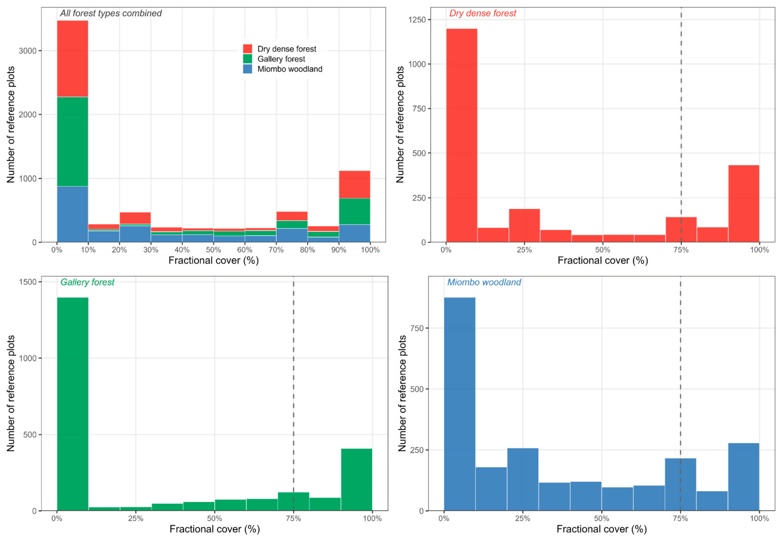
Reference data were generated through systematic visual photo-interpretation of 2333 virtual sample plots (0.25 ha; 50 × 50 m) using Collect Earth Online [32]. The plots were distributed across Lualaba Province using a stratified random sampling design proportional to the spatial extent of each forest type: Dry dense forest, Gallery forest, and Miombo woodland. This approach ensured balanced coverage of the compositional gradient and reduced overestimation bias [25,33]. The final sample comprised 758 plots (32.5%) classified as Dry dense forest, 794 plots (34.0%) as Gallery forest, and 781 plots (33.5%) as Miombo woodland. The frequency distribution of fractional cover values across all plots, showing the compositional structure of the training dataset by forest type, is presented in Appendix E (Figure A1). Within each plot, fractional cover per forest type was computed from systematic point interpretation of very high-resolution imagery, yielding continuous compositional estimates compatible with Sentinel-2 pixel-level modelling [33]. The complete training dataset, comprising spectral predictors and fractional cover values for all 2333 reference plots, is provided in Table S1 (Supplementary Materials). The reliability of the photo-interpreted data was assessed using an independent field inventory comprising 60 plots (50 × 50 m; 20 per forest type) collected across Lualaba Province between June and August 2025. Strong agreement was observed between photo-interpreted and field-based estimates (mean R2 = 0.754; mean RMSE = 1.30 percentage points), confirming the robustness of the interpretation protocol. Detailed per-class accuracy metrics and potential biases are provided in Appendix B.
2.2.2. Sentinel-2 Predictors
Satellite data were sourced from the Sentinel-2 MSI Level-2A surface reflectance collection (COPERNICUS/S2_SR_HARMONIZED) and processed using Google Earth Engine (GEE) [34]. Images were limited to April–November 2025 and filtered to include observations with fewer than 10% cloud cover; a total of 1618 images meeting these criteria were retained; full acquisition metadata are provided in Table S2 (Supplementary Materials). The wet season (December–March) was excluded due to persistent cloud interference and potentially reduced spectral separability among forest types [31]. A pixel-wise median composite was generated from all valid observations, and all 20 m bands were resampled to 10 m using bilinear interpolation for spatial consistency across predictors.
Predictor selection followed a structured, group-based evaluation described in full in Appendix A (Table A1). Fourteen candidate predictor sets were predefined by combining five thematic groups: (i) Sentinel-2 spectral bands, (ii) vegetation indices, (iii) texture metrics from grey-level co-occurrence matrices (GLCM), (iv) topographic variables, and (v) engineered features. These sets ranged from simple single-family configurations (such as spectral or vegetation-only) to complex composite and engineered models (Table A1). Each set was evaluated via spatial block cross-validation (K = 5 folds; 2000 m blocks) applied to all 2333 reference plots, ensuring that predictor selection was based on held-out spatial test performance rather than training fit and therefore remained free of data leakage [26,35]. Performance metrics included R2, RMSE, and MAE. Predictor sets were ranked by mean cross-validated R2, with the eco_medium configuration (13 variables) serving as a composite baseline. The optimal predictor set was identified at the inflexion point of the R2 convergence curve, defined a priori as the point beyond which additional variables yield marginal improvements of less than ΔR2 = 0.01 [35,36]. This criterion identified the eco_texture configuration (15 variables) as optimal, achieving the highest cross-validated performance (R2 = 0.641) with a slight but consistent improvement over the eco_medium baseline (R2 = 0.636; ΔR2 = +0.005). Crucially, all subsequent configurations with additional variables yield equal or lower R2 (ΔR2 ≤ 0; Table A2), confirming that eco_texture represents the optimal trade-off between predictive performance and model complexity.
The chosen eco_texture predictor set comprised 15 variables: eight Sentinel-2 reflectance bands (B3, B4, B5, B6, B7, B8, B11, B12), five vegetation indices (NDVI, EVI, NDMI, NBR, CV-NDVI), and two GLCM texture metrics (NDVI contrast and NDVI entropy). Red-edge and SWIR bands captured chlorophyll content and canopy moisture, respectively. B8A was evaluated but excluded from the optimal predictor set as its inclusion yielded no meaningful performance gain (ΔR2 ≤ 0; Appendix A, Table A2), consistent with the inflection-point selection criterion applied here; CV-NDVI added phenological contrast; and GLCM texture metrics resolved fine-scale canopy heterogeneity beyond the reach of spectral predictors alone.
2.2.3. Forest Mask
The forest mask serves as a spatial constraint for the MONN: because the softmax output layer distributes predicted cover exclusively among the three forest types, applying the model to non-forest pixels would yield compositionally invalid outputs. The mask therefore restricts predictions to pixels where the compositional framework is ecologically meaningful.
A binary forest mask was derived from a supervised Random Forest classification (500 trees) applied to a Sentinel-2 composite using 10 spectral bands (B2–B12) and NDVI, processed in GEE [34]. Dry dense forest, Gallery forest, and Miombo woodland were merged into a single forest stratum [25]. The resulting mask achieved a Producer’s Accuracy of 92.4% and a User’s Accuracy of 90.9%, indicating reliable spatial delineation with no evidence of systematic bias in forest area estimation. The full accuracy assessment is provided in Appendix D.
2.3. Random Forest Normalised Approach
Three independent Random Forest regression models were trained, one per forest type (RF_Dry dense, RF_Gallery, RF_Miombo), using the ranger package in R [37]. Hyperparameters followed well-established regression defaults: 500 trees, mtry = ⌊√P⌋ = 3 candidate variables per split, and a minimum node size of 5 [38]. Hyperparameter tuning was deliberately omitted for three reasons. First, the default mtry = ⌊√P⌋ is consistently recommended for regression tasks and rarely yields substantial gains with moderate-sized datasets [39]. Second, nested cross-validation required for unbiased tuning within a spatial block CV framework would have introduced prohibitive computational overhead with five spatial folds and three simultaneous models. Third, and most importantly, fixing hyperparameters to identical defaults across both models ensures that observed performance differences between RF and MONN reflect architectural differences rather than tuning advantages—the comparison that is of primary scientific interest in this study. Exploratory tests varying mtry (⌊√P⌋, ⌊P/3⌋, ⌊P/2⌋) and minimum node size (1, 5, 10) on a single spatial fold yielded no consistent R2 improvement greater than 0.003, corroborating the decision to retain the default parameterisation.
A fundamental structural limitation of this independent RF approach is that each model is trained in isolation, without conditioning on the predictions of the other forest types. This violates the compositional constraint: raw RF outputs are unconstrained continuous values that may fall outside [0, 1] and whose sum across the three types need not equal one [40]. This is precisely the architectural weakness that the MONN addresses intrinsically via its softmax output layer. To make RF outputs compositionally valid for comparison, a pixel-wise post hoc normalisation was applied: each raw prediction was clipped to [0, 1], then divided by the sum of the three clipped values, yielding proportions that sum to exactly one at each pixel. When the total of clipped predictions was zero, all proportions were set to zero. This normalisation step is a pragmatic correction rather than a principled compositional model.
2.4. Multi-Output Neural Network
The MONN was implemented as a fully connected feedforward neural network (FCNN) in Keras—a per-pixel architecture chosen to match RF’s input structure, ensuring that performance differences reflect the softmax constraint alone. The objective was therefore not to maximise predictive performance, but to isolate the effect of compositional constraints under identical predictor information. This choice is further justified by the provincial-scale prediction scope (52.2% of Lualaba Province classified as forested after mask application). The architecture comprised four hidden layers with progressively decreasing capacity (512–256–128–64 units), designed to compress the 15-variable spectral and textural input into a compact compositional representation. Each of the first three hidden layers was followed by batch normalisation [41], ReLU activation, and dropout (rates: 0.30, 0.25, and 0.20, respectively) to regularise training and prevent overfitting [42]. The fourth hidden layer used ReLU activation without dropout. The output layer comprised three neurons—one per forest type—activated by a softmax function. This directly encodes the compositional constraint within the network: outputs are strictly positive and sum to exactly 1, without any post hoc correction [43].
The model was trained using the Adam optimiser [44] with an initial learning rate of 0.001 and a batch size of 32. Training ran for a maximum of 300 epochs with two adaptive callbacks: early stopping (patience = 20 epochs, monitoring validation loss, restoring best weights) and learning rate reduction on plateau (factor = 0.5, patience = 8 epochs, minimum learning rate = 10−6). A 15% validation split was held out from the training fold at each cross-validation iteration to monitor generalisation. The loss function was the Kullback–Leibler divergence between observed and predicted compositional distributions. This is more semantically appropriate than mean squared error for probability outputs: it measures the information cost of substituting the true composition with the predicted one and more heavily penalises errors on dominant forest types. Complete architecture specifications and training hyperparameters are provided in Appendix C.
2.5. Spatial Block Cross-Validation
Both models were evaluated within an identical spatial block cross-validation framework using the blockCV package [28], with K = 5 folds and a block size of 2000 m. The block size was determined as the minimum distance that ensured spatial independence between the training and test sets, as verified by the absence of residual spatial autocorrelation across folds (Moran’s I; [27]). Applying the same fold structure to both RF and MONN ensures that performance differences reflect architectural properties alone.
Predictive variability across folds was quantified as the inter-fold coefficient of variation (CV), computed pixel-by-pixel as the ratio of the standard deviation to the mean of the fivefold-specific predicted cover values, expressed as a percentage. This produces a spatially explicit map of prediction stability under geographic resampling—a measure of how consistently the model predicts across different spatial partitions of the data, not a probabilistic uncertainty estimate in the Bayesian sense. Zones of high inter-fold CV indicate configurations sensitive to the spatial composition of the training set.
2.6. Performance Metrics
Model performance was quantified using three complementary metrics averaged across the K = 5 spatial folds: the coefficient of determination (R2), root mean square error (RMSE), and mean absolute error (MAE) [45]. To assess performance under compositionally demanding conditions, test pixels were stratified into three classes based on the maximum observed cover proportion of any single forest type: pure pixels (dominant proportion > 75%), moderately mixed pixels (50–75%), and highly mixed pixels (<50%). This stratification captures the gradient from spectrally coherent to compositionally ambiguous pixels and allows evaluation of how both models respond to increasing subpixel heterogeneity.
Following cross-validation, both models were retrained on the complete 2333-plot dataset using the same architecture and hyperparameters to produce the final composition maps applied to the Lualaba Province raster stack.
2.7. Continuous Composition and Categorical Classification: Metrics and Framework
Categorical land-cover classification assigns each pixel to a single discrete class, thereby retaining only the dominant cover type and discarding information on minority cover types [46,47,48]. In contrast, continuous compositional mapping represents each pixel as a vector of proportional cover values that sum to unity, providing a more complete description of within-pixel heterogeneity [12,49]. In this study, we adopt this compositional framework to better capture the structural complexity of forest landscapes, where multiple vegetation types frequently coexist within a single pixel.
Each pixel is described by the proportional cover of three forest types—Dry dense forest, Gallery forest, and Miombo woodland—denoted wc_A, wc_B, and wc_C, respectively. These proportions take values in [0, 1], where 1 corresponds to 100% cover, and are constrained to sum to unity:
wc_A + wc_B + wc_C = 1.
This constant-sum constraint defines the data as compositional in nature, implying that the components are not independent and must be interpreted within a relative framework [40]. A minimum presence threshold of 5% was applied to avoid spurious low-proportion contributions inherent to soft classification outputs. The sensitivity of this threshold was evaluated (3–10%) to ensure that it does not drive the observed compositional patterns (Appendix F and Appendix G). More generally, let S denote the number of cover types in the compositional vector (S = 3 in this study), allowing the use of general expressions such as 1/S and ln(S) in the formulation of compositional metrics.
To characterise compositional structure and evaluate the implications of reducing continuous information to categorical labels, two complementary metrics are derived: (i) the dominant class proportion and (ii) Shannon compositional entropy. A third quantity, categorical information loss, is derived directly from the proportion of the dominant class and is included as an interpretive aid rather than as an independent metric. These quantities describe complementary aspects of compositional variation, and their relationships are examined in Appendix G.
- -
- The dominant class proportion (Pdom) is defined as:
Pdom = max(wc_A, wc_B, wc_C).
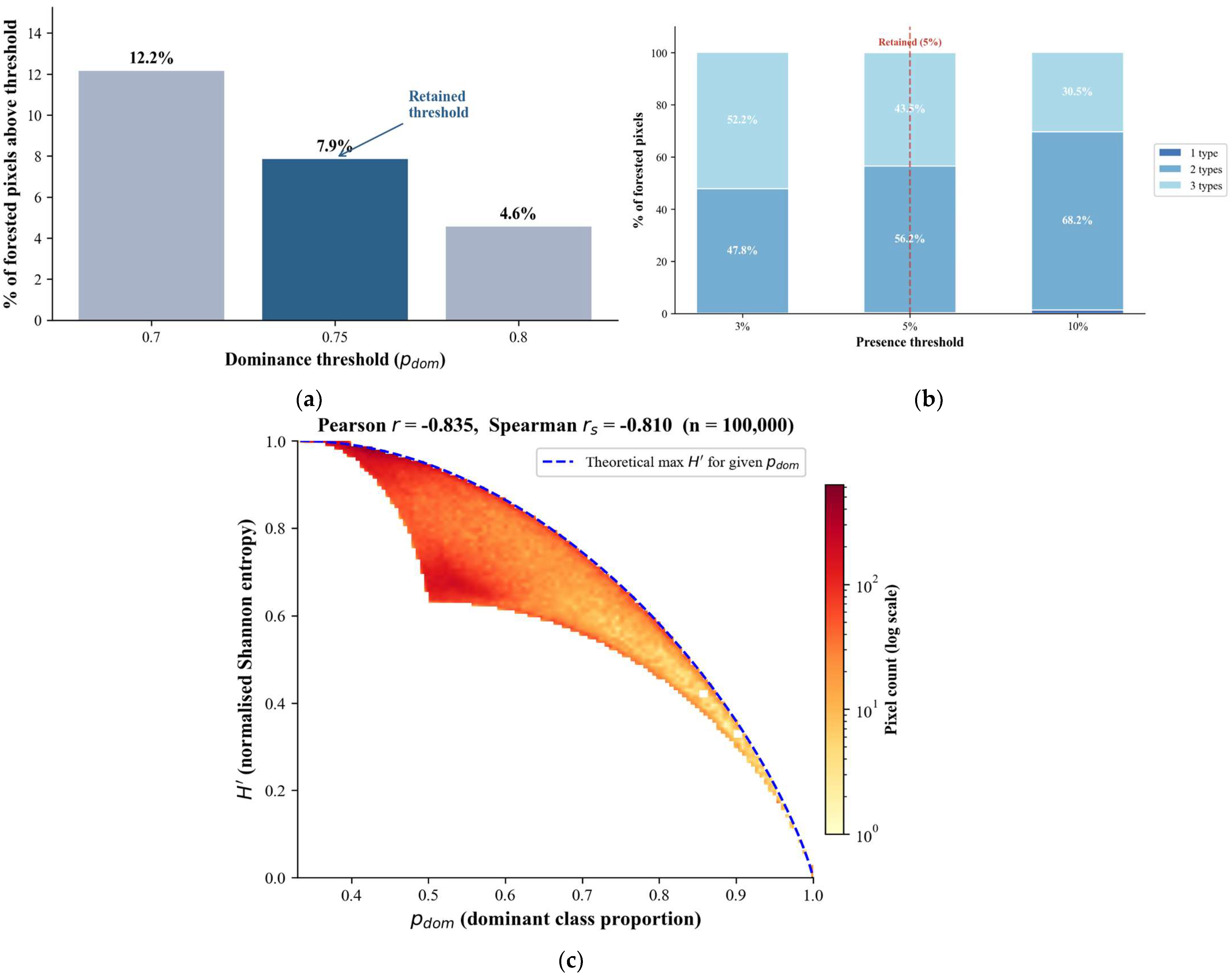
This metric represents the only quantitative compositional information retained under categorical classification, ranging from 1/S = 1/3 (33.3%) to 1 (100%), corresponding to complete dominance by a single class. To identify pixels for which categorical attribution remains meaningful, a dominance threshold is required. Because no universal threshold exists, a sensitivity analysis was conducted using three candidate values (0.70, 0.75, and 0.80). For computational efficiency, the analysis was performed on a representative subset of pixels, whereas all summary statistics reported in the main results are derived from the full dataset. Lower thresholds (e.g., 0.50–0.60) were not considered, as they would classify substantially mixed pixels as dominant, thereby reducing interpretability. The sensitivity analysis showed that the proportion of pixels classified as dominant decreases from 12.2% at 0.70 to 4.6% at 0.80, a reduction of 7.6 percentage points. This rapid contraction confirms that lower thresholds are overly permissive, while thresholds above 0.80 become overly restrictive. A threshold of Pdom > 0.75 was therefore retained as a pragmatic compromise, ensuring that only clearly dominated pixels are identified while preserving sufficient spatial representation. The threshold, therefore, serves as a reporting criterion rather than a modelling assumption, and does not affect the central conclusions regarding the prevalence of compositional mixing.
- -
- The categorical information loss (Ecat) is derived directly from the dominant proportion as its complement:
Ecat = 1 − Pdom
This quantity represents the proportion of within-pixel cover assigned to non-dominant forest types, which is discarded when a categorical label is applied. It is explicitly defined as a linear transformation of Pdom (its arithmetic complement) and is therefore not an information-theoretic measure in the Shannon or Kullback–Leibler sense: it does not quantify distributional uncertainty or the complexity of the full cover vector. The distributional structure of within-pixel mixing—including how cover is redistributed among non-dominant types—is captured independently by Shannon compositional entropy H′ (Equation (5)), which is sensitive to the full probability vector and constitutes the primary metric of compositional complexity in this framework. Ecat is retained as a directly interpretable summary of the magnitude of categorical loss at the pixel level, complementary to H′ rather than redundant with it. Together, these two quantities characterise complementary but not independent aspects of compositional structure: Ecat reflects the share of composition lost, while H′ reflects how that remaining composition is distributed. The sensitivity analyses presented in Appendix F and Appendix G confirm that conclusions are robust to threshold choice and that the metric combination is sufficient to characterise the compositional structure of the landscape without requiring additional divergence measures.
To characterise the internal distribution of cover among all classes, Shannon entropy is computed as [50]:
with the convention 0·ln(0) = 0. Entropy ranges from 0 (complete dominance) to ln(S) = ln(3) ≈ 1.099, corresponding to maximum compositional mixing. Entropy is normalised following Pielou [51]:
Due to the constant-sum constraint of compositional data, H′ and Pdom are inherently related but capture different aspects of compositional structure. A strong negative relationship between Pdom and H′ is expected and was confirmed empirically (Appendix G). Principal component analysis applied to CLR-transformed proportions revealed that PC1, accounting for 85.0% of compositional variance, primarily contrasts Gallery forest against Dry dense forest and Miombo woodland (loadings: Gallery = +0.777, Dry dense = −0.605, Miombo = −0.172) and shows only weak correlation with P~dom~ (Pearson r(PC1, Pdom) = −0.21). PC2 (15.0% of variance) reflects a contrast between Miombo woodland and the other two forest types (Miombo loading = +0.798) and is more strongly associated with dominance (Pearson r = 0.41). These results suggest that the dominance gradient captured by Pdom is a secondary rather than primary axis of compositional variation: the dominant structural gradient reflects the redistribution of cover among forest types rather than an overall increase or decrease in mixing. Full details are provided in Appendix G.
3. Results
3.1. Model Performance: Random Forest Versus Neural Network
Spatial block cross-validation results are presented in Figure 2. The MONN performed comparably to RF overall (R2: 0.630 vs. 0.648; RMSE: 0.229 vs. 0.224; ΔR2 = −0.018), with MONN outperforming RF in three of five spatial folds. The fold-level difference was not statistically significant (Wilcoxon signed-rank test, W = 5, p = 0.625), reflecting the modest nature of the performance gap. The advantage of MONN was most pronounced for Dry Dense forest (ΔR2 = +0.025), where compositional constraints are most informative. Inter-fold variability was similar between models, indicating comparable spatial stability. The zero-sum edge case in RF normalisation did not occur across the full forested area, confirming that this correction introduces no bias in the reported metrics.
Figure 2.
Observed versus predicted woodcover for RF (left) and MONN (right) across Miombo woodland, Gallery forest, and Dry Dense forest. Hexagonal bins represent point density from spatial block cross-validation (k = 5, block = 2000 m). The clustering of predictions near zero is structurally expected in a sampling design stratified by forest type, where each type is dominant in a minority of pixels and absent or marginal in the majority, naturally producing a high density of near-zero predictions for each non-dominant type. This reflects the sampling design structure, not a model artefact. Solid line = OLS regression (shaded = 95% CI); dashed line = 1:1 reference. Metrics computed on held-out test folds only.
Performance stratified by pixel composition class (Table 1) reveals a sharp discontinuity. Both models perform well on pure (R2 ≈ 0.65) and moderately mixed pixels (R2 ≈ 0.63), with the MONN showing marginal gains in both classes (ΔR2 = +0.014 and +0.010, respectively). However, both models show near-zero explanatory power for highly mixed pixels (RF R2 = 0.008 ± 0.004; MONN R2 = 0.007 ± 0.006; dominant proportion < 50%), despite similar RMSE values across all classes. This sharp R2 collapse, with no corresponding increase in RMSE, indicates that both models default to predicting near the mean in highly mixed pixels, capturing magnitude but not compositional variance. Critically, highly mixed pixels represent 43.0% of the forested area (Table 1), confirming that this is not a marginal failure mode but the dominant predictive condition.
Table 1.
Model performance metrics across pixel composition classes. Values represent the mean ± standard deviation calculated over K = 5 spatial folds. Note: the percentage of forested area per class reflects the distribution of test pixels across the five spatial cross-validation folds, not the provincial raster; landscape-level proportions from MONN predictions are reported in Section 3.3 and Table 2. RMSE is expressed as a dimensionless proportion (cover values in [0, 1]). ΔR2 = MONN R2 − RF R2.
Table 2.
Pixel mixture structure across the forested area of Lualaba Province. Panel (A) reports the distribution of pixels by mixture class, defined by the number of forest types exceeding the 5% softmax presence threshold. Panel (B) reports the sensitivity of this classification to threshold choice.
3.2. Spatial Distribution of Predicted Woodcover Composition
The MONN produced spatially consistent woodcover composition maps for the 52.2% of Lualaba Province classified as forested (Figure 3a–c). Miombo woodland dominated the landscape in mean cover, followed by Dry dense forest and Gallery forest, the latter showing high spatial variability consistent with its linear riparian distribution. The RGB ternary map (Figure 3d) reveals a fine-scale mosaic in which Dry dense forest and Miombo woodland co-occur across the central and southern provinces. In contrast, Gallery forest traces a sparse but persistent network along drainage systems, a spatial structure that no single categorical map can capture without substantial information loss.
Figure 3.
Spatial predictions of woodcover composition and prediction uncertainty across forested pixels of Lualaba Province, derived from the MONN. (a–c) Predicted proportional woodcover (%) per forest type; pixel values sum to 100% at each location. (d) Composition-weighted coefficient of variation (CV = σ_folds/ × 100) across five spatially blocked cross-validation folds; colour scale saturated at the 85th percentile to reveal spatial gradients within the low-uncertainty range. (e) RGB ternary composite showing compositional mixing among forest types. Pure Miombo woodland pixels (blue) are scarce; the predominance of magenta–purple hues indicates that Miombo mostly occurs as a mixture with Dry dense forest.
Inter-fold predictive variability remained low province-wide (weighted coefficient of variation, CV = 4.7%), confirming the spatial stability of MONN outputs under geographic resampling. The Spearman correlation between CV and Shannon entropy was negative (ρ = −0.298, p < 0.001): inter-fold variability concentrates in the rarest, most spectrally pure pixels, not in the mixed pixels that dominate the landscape. This pattern reflects two compounding mechanisms: the underrepresentation of pure-class pixels in the training dataset and the potentially higher intrinsic spectral variability within spectrally pure types, such as dense forests.
3.3. Compositional Mixing as the Dominant Landscape Condition: Implications for Categorical Mapping
Compositional mixing characterises the forested landscape of Lualaba Province. The mean dominant-class proportion was 56.2%, implying that categorical attribution discards, on average, 43.8% of within-pixel compositional information (Figure 4a–c). Only 7.9% of forested pixels exceeded the 75% purity threshold, while 28.8% fell below 50%—the level at which single-label assignment becomes ecologically arbitrary (Figure 4b). Shannon entropy averaged 74.1% of its theoretical maximum (Figure 4d), confirming that near-complete mixing, rather than dominance, is the prevailing structural state. Across 92.1% of pixels, no single forest type reached the purity level required for defensible categorical attribution.
Figure 4.
Spatial patterns of compositional dominance and within-pixel heterogeneity across forested pixels in Lualaba Province. (a) Dominant class proportion (Pdom = max (wc_A, wc_B, wc_C)), ranging from 1/3 (33%) to 1 (100%), where higher values indicate stronger dominance of a single forest type. (b) Frequency distribution of Pdom across all forested pixels; vertical lines mark reference thresholds at 50%, 67%, and 75%, and shaded regions highlight increasing levels of dominance. The red and green shaded regions, matched by the corresponding legend patches, denote pixels with p dom < 50% and p dom > 75%, respectively. (c) Categorical residual (Ecat = 1 − Pdom), representing the proportion of non-dominant cover excluded under categorical classification; higher values indicate greater omission of within-pixel composition. (d) Shannon compositional entropy (H), ranging from 0 to ln(3) ≈ 1.10, reflecting the evenness of cover distribution among forest types, with higher values indicating more heterogeneous compositions. Together, these panels illustrate the structural dominance of compositional mixing and the resulting magnitude of categorical information loss.
Virtually no pixel was compositionally pure: only 0.3% of forested pixels showed a single dominant forest type exceeding the 5% presence threshold (Table 2, Panel A). Two-type mixtures accounted for 56.2% of the area and three-type mixtures for 43.5%—though these proportions are threshold-dependent and shift substantially across the 3–10% range (Table 2, Panel B); only the near-absence of mono-type pixels (0.1–1.4%) is robust across all thresholds tested, confirming that the main conclusion does not depend on threshold selection.
Across all three forest types, mean dominant proportions ranged from 0.529 (Miombo woodland) to 0.609 (Dry dense forest), with entropy following the inverse pattern (Table A7). Miombo woodland, which covers 50.3% of the forested area, showed the highest entropy (H′ = 0.792), reflecting extensive compositional overlap with adjacent types. A Mann–Whitney test confirmed that nominally pure pixels (Pdom > 0.75) exhibited significantly higher inter-fold predictive variability than mixed pixels (CV: 4.77% vs. 4.39%; U = 173,526,728, p < 0.001): prediction is least stable precisely where categorical attribution appears most justified.
All reported proportions should be interpreted in relation to the chosen presence (5%) and dominance (75%) thresholds.
4. Discussion
4.1. MONN Versus RF: Consistent Gains in a Compositionally Constrained Regression Task
The MONN consistently outperformed RF across all forest types and folds (R2: MONN = 0.648 vs. RF = 0.630; RMSE: MONN = 0.224 vs. RF = 0.229). The gain, while modest in absolute terms, is architecturally principled: the softmax output layer encodes the unit-sum constraint directly into the forward pass, enabling the model to learn the three forest-type proportions jointly rather than independently [19,21,22,43]. This contrasts with the RF approach, where compositional validity is imposed post hoc via normalisation, a correction that cannot recover the interdependencies lost during training three separate models. This correction is moreover structurally benign: the forest mask restricts predictions to pixels where at least one forest type is present, and 99.7% of pixels contain two or more forest types (Table 2), making null row sums structurally improbable. The gain is most pronounced for Dry dense forest (ΔR2 = +0.025), the type with the sharpest ecological boundaries and thus the most informative compositional constraint. These results align with Allred et al. [21] and Schug et al. [22], who showed that jointly trained architectures outperform independent regression models for fractional cover mapping in heterogeneous landscapes.
The overall R2 of 0.648 is commensurate with comparable frameworks operating under similar data constraints: Reiner et al. [18] reported R2 values of 0.55–0.70 for continent-wide African tree cover mapping from a single-date composite, and Abdou Amadou et al. [11] obtained comparable accuracy for fractional woodcover in West African agropastoral landscapes using Sentinel-2 and Random Forest regression. Lluïsà et al. [52] achieved R2 values up to 0.92, but under substantially more favourable conditions: synthetically mixed training data that span the full spectral mixing space by design, and dense multi-date time series providing phenological separability unavailable in a single-season composite. The performance gap relative to Lluïsà et al. [52] therefore reflects structural differences in data availability rather than a model shortcoming. The near-zero R2 on highly mixed pixels—defined here as pixels where no single forest type exceeds 50% cover (43.0% of the training sample; Table 1), corresponding largely to the 43.5% of the provincial raster exhibiting three-type mixtures (Table 2)—reflects a spectral identifiability limit rather than a model flaw: when multiple forest types co-occur at sub-pixel scale with overlapping spectral signatures, no single-date optical model can reliably partition their contributions [53]—and crucially, these are precisely the pixels where categorical attribution is most inadequate and continuous compositional mapping most necessary. The underrepresentation of intermediate proportions in the training dataset (Appendix E) may additionally contribute to mean-regressive predictions in this class, though it is not the primary driver of the R2 collapse: the convergence of both RF and MONN towards near-zero explanatory power—despite their fundamentally different learning mechanisms—suggests a limitation arising primarily from the information content of the predictors rather than from model structure alone. This behaviour is consistent with theoretical limits of linear spectral unmixing in optically similar vegetation types. Unlike categorical approaches, the MONN makes this structural ambiguity spatially explicit rather than concealing it under a single class label. For continuous vegetation dynamics monitoring, this transparency is precisely what allows gradual compositional shifts to be tracked over time [54].
4.2. Compositional Mixing as the Dominant Landscape Condition
The pixel-by-pixel quantification of categorical information loss constitutes the central contribution of this study. To our knowledge, no previous work has formally mapped Ecat at the provincial scale in a tropical African landscape; the convergence of three independent metrics and the low province-wide CV (4.7%; Section 3.2) confirms that these patterns are structural rather than artefactual. The sensitivity analysis confirmed that the proportion of pixels classified as dominant decreases sharply from 12.2% at 0.70 to 4.6% at 0.80 (Appendix G), with 0.75 representing the inflection point of this contraction. Similarly, the near-absence of mono-type pixels (0.1–1.4%) was robust across the full presence threshold range tested (Appendix G), confirming that the compositional mixing conclusion does not depend on either threshold choice.
This result extends a widely acknowledged but rarely formalised limitation in remote sensing. Fernandes [49] identified sub-pixel mixing as the primary source of categorical error in heterogeneous landscapes; Herold et al. [55] showed that global products systematically disagree in transition zones; and Schug et al. [22] confirmed that subpixel fraction mapping overcomes these limitations where patch sizes fall below sensor resolution. Castle et al. [7] recently demonstrated that global forest dataset incongruence translates directly into high uncertainties for conservation and climate policy—an effect our results suggest is structurally unavoidable in landscapes where 92.1% of pixels cannot be unambiguously attributed to a single class. Global categorical map incongruence for forest cover in the DRC region has also been quantified at scale [56], and Sexton et al. [6] showed that even 30 m global products diverge substantially in transitional canopy zones of the kind that dominate Lualaba Province. Picard et al. [5] demonstrated that even the Congo Basin dense forest is a complex structural mosaic; our study extends this conclusion to the drier, miombo-dominated landscapes of southern DRC and, crucially, provides the first pixel-level quantification of the information cost of categorical attribution at full provincial resolution.
The per-type patterns are ecologically coherent. Miombo woodland dominates the landscape yet shows the lowest compositional purity (Table 2), consistent with its open-canopy structure and the co-occurrence of dry, dense forest species along edaphic gradients [9]. Dry dense forest shows the highest purity, reflecting its sharper ecological boundaries on better-drained mid-slope soils [10]. Gallery forest transitions seamlessly into both adjoining formations along hydrological gradients, boundaries that are invisible to categorical maps but spatially explicit in continuous compositional outputs. These ecological gradients match those identified by Picard et al. [5] as primary drivers of forest-type distribution in Central Africa.
The joint behaviour of Pdom, Ecat, and H clarifies the structure of compositional variation across the landscape. PCA applied to CLR-transformed proportions revealed that the primary axis of variation (PC1, 85.0% of variance) reflects the substitution of Gallery forest by Dry dense and Miombo woodland, and is largely independent of dominance level (r = −0.21 with Pdom). The dominance gradient is instead associated with PC2 (15.0% of variance; r = 0.41), confirming that overall mixing intensity is a secondary structural axis. Shannon entropy shows a strong negative relationship with Pdom (r = −0.835), consistent with the constant-sum constraint of compositional data. Ecat, as its linear complement, provides no independent structural information but facilitates direct interpretation of compositional loss. Together, these metrics define a hierarchical description of compositional structure where the dominant axis captures forest-type substitution, and the secondary axis captures mixing intensity—a distinction invisible to categorical maps.
4.3. Limitations and Perspectives
Three limitations bound the scope of this study without undermining its central contribution. First, although the photo-interpretation protocol was validated against independent field plots (R2 = 0.754; Section 2.2.1), the MONN compositional maps have not been validated against independent biomass measurements at the pixel level across the full provincial extent, a prerequisite for operational use in carbon accounting. The inter-fold CV map (Section 2.5) provides a spatially explicit measure of prediction stability under geographic resampling—the uncertainty dimension most directly relevant to the central objective of this study. Full probabilistic uncertainty quantification via MC-Dropout inference [57], separating aleatoric from epistemic uncertainty, is identified as a priority for future operational applications (Section 4.4). Second, the softmax output layer structurally prevents compositionally pure pixels. Because the exponential function never reaches zero, every forest type receives a strictly positive weight at every pixel, imposing a soft ceiling on Pdom and a soft floor on H′. The reported metrics (mean Pdom = 56.2%; H′ = 74.1% of Hmax) therefore reflect both genuine landscape mixing and this architectural constraint. However, quantification of the observed logit distribution confirms that the soft floor is negligible in practice: the minimum predicted proportion across all training plots is 0.0001% (maximum logit difference = 12.86), three orders of magnitude below the 5% presence threshold, and therefore indistinguishable from true absence at any ecologically meaningful scale. Recomputing all compositional metrics after truncating values below 0.001% produced changes of exactly zero across all training plots, confirming that the reported mixing patterns are ecological rather than architectural in origin. Third, Shannon entropy conflates genuine ecological mixing with residual model uncertainty; disentangling these two sources would require a full Bayesian framework, for instance, MC-Dropout inference [57], to separate aleatoric from epistemic uncertainty. The inter-fold CV reported here captures only the latter and should not be interpreted as a proxy for the former.
Two secondary limitations concern threshold choices and temporal scope. The 5% presence threshold used to define meaningful forest-type contributions lacks formal ecological justification. Its sensitivity was evaluated across 3–10%: the qualitative conclusion of near-universal mixing is robust (mono-type pixels: 0.1–1.4% across the range), but the exact partition between two- and three-type pixels varies substantially (Appendix G, Figure A3) and should be treated as an order-of-magnitude indicator rather than a precise ecological quantity. Similarly, the dominance threshold of Pdom > 0.75 is a pragmatic compromise, confirmed by sensitivity analysis (12.2% to 4.6% across 0.70–0.80; Appendix G, Figure A3), rather than a universal ecological criterion. Models were also trained on 2025 imagery; transferability across years remains untested, given Lualaba’s pronounced interannual rainfall variability [30], and spatial block cross-validation does not fully capture spectral non-stationarity across a climatically diverse area of 120,000 km2 [58,59].
The carbon and biodiversity implications of this compositional mixing are quantifiable. Ryan et al. [9] reported aboveground carbon stocks of 26–34 Mg C ha−1 for miombo woodland in Mozambique and substantially higher values for structurally denser dry forest formations—a difference of the same order as the within-pixel compositional uncertainty documented here. When categorical maps assign a pixel to Miombo woodland, although it contains 40% Dry dense forest, the applied biomass equation underestimates carbon by a systematic margin that cannot be corrected post hoc without knowing the true fractional composition. Réjou-Méchain et al. [60] showed that propagating such errors across landscape-scale biomass upscaling compounds uncertainties substantially, particularly in heterogeneous tropical systems. Similarly, Higginbottom and Symeonakis [61] demonstrated that vegetation index trajectories underestimate degradation severity in mixed-canopy landscapes because declining contributions from one formation are partially masked by stable or recovering contributions from another—precisely the dynamic that continuous compositional maps would make visible at the pixel level. Grantham et al. [62] quantified the extent of anthropogenic modification in tropical forests and noted that global categorical products chronically underestimate degradation in the miombo belt; our results provide a structural explanation for that underestimation. Finally, Wan et al. [63] demonstrated that satellite-derived canopy height and aboveground biomass maps at 10 m resolution are achievable in African tropical forests but require compositionally resolved input layers—an argument for continuous compositional outputs of the kind produced here as precursor data for REDD+ biomass estimation. These implications remain inferential and should be confirmed using biomass-calibrated datasets.
While the composite integrates observations from multiple phenological stages, median compositing collapses temporal trajectories into a single synthetic observation. Consequently, phenological dynamics are only represented indirectly through temporal variability metrics such as CV-NDVI, and future work using explicit multi-temporal sequences may further improve discrimination among mixed forest compositions. Priority perspectives include multi-date extensions to detect gradual compositional changes along the Lobito corridor [3]; integrating GEDI spaceborne LiDAR to improve discrimination between structurally similar formations [64]; multi-temporal stacking across years and SAR integration (e.g., Sentinel-1 backscatter) to improve separability among structurally similar forest types, potentially alleviating the R2 collapse observed for highly mixed pixels; and CNN or Vision Transformer architectures that exploit Sentinel-2 spatial context [5,19,21,22]. Future sampling strategies could nonetheless benefit from targeted plot placement in transitional zones to better characterise the spectral behaviour of intermediate compositions. None of these limitations alters the core result: the continuous compositional framework formally quantifies, at the provincial scale and full spatial resolution, the information that categorical maps structurally cannot convey in highly mixed landscapes such as Lualaba. This quantification is robust to the threshold and architectural choices examined here.
4.4. Implications for Vegetation Dynamics Monitoring, Carbon Assessment, and Biodiversity Evaluation
Continuous compositional outputs preserve three types of information that categorical products are structurally unable to convey: the simultaneous proportions of minority forest types within each pixel, the spatial gradient of compositional transitions, and the per-pixel intensity of mixing. Full probabilistic uncertainty quantification—separating aleatoric from epistemic uncertainty via MC-Dropout inference [57]—remains a methodological priority for future operational applications of this framework. These translate into direct operational relevance across three priority domains for forest management in the DRC.
First, in biomass and carbon accounting, mixed-formation pixels deviate systematically from single-type allometric relationships, causing bias that accumulates across landscapes [60,64]. Wan et al. [63] confirmed that forest-type mixing remains the primary source of uncertainty in 10-m carbon stock estimates across African dense forests. The per-pixel forest-type proportions produced by the MONN provide the input needed to apply type-specific biomass models, directly reducing this bias within REDD+ accounting frameworks [23,24].
Second, in forest degradation monitoring, gradual compositional shifts—the progressive replacement of dry dense forest by Miombo woodland within pixels—precede and are more ecologically informative than detectable cover loss, yet remain invisible to categorical change detection [4,61]. The continuous approach converts these dynamics into quantifiable, spatially explicit signals. This capacity is especially critical in Lualaba Province, where the development of the Lobito economic corridor is expected to intensify land-use pressure and accelerate forest degradation across the region in the coming years [3]. Continuous compositional maps provide the baseline needed to detect and attribute these changes before they cross the threshold of categorical detectability.
Third, in biodiversity modelling, species richness in miombo landscapes peaks at compositional transition zones precisely the zones that categorical maps collapse into a single label [9,62]. The Shannon entropy map produced here serves as a direct spatial proxy for transition zone intensity, enabling targeted biodiversity assessments without additional field surveys.
5. Conclusions
This study offers the first large-scale assessment of how much categorical information is lost in mapping tropical forest cover. In Lualaba Province, 92.1% of forest pixels do not meet the 75% purity threshold required for unambiguous categorical attribution. On average, categorical classification omits 43.8% of within-pixel compositional information, and Shannon entropy reaches 74.1% of its theoretical maximum. Together, these metrics confirm that compositional mixing is the dominant structural condition of this landscape, rendering categorical attribution inadequate across most forested pixels. The Multi-Output Neural Network, which encodes the unit-sum constraint directly via a softmax layer, outperforms separate Random Forest models and uniquely makes this information loss spatially explicit and measurable. This has practical implications: categorical forest maps in Lualaba and similar miombo landscapes are expected to introduce bias in carbon stock estimates by mixing forest types with contrasting biomass—an inference that remains to be confirmed against biomass-calibrated field data—hide early signs of forest degradation by masking gradual compositional shifts, and reduce biodiversity transition zones to uniform labels. As land-use pressure grows, the costs of this misrepresentation will increase. Continuous compositional mapping represents the appropriate operational framework for landscapes where mixing is the structural norm rather than the exception. Future work should focus on: first, multi-date mapping to detect gradual compositional changes as early indicators of degradation before they become detectable via categorical change detection; second, integrating GEDI LiDAR canopy height data to better distinguish structurally similar formations at intermediate cover levels and support type-specific biomass estimates aligned with REDD+ standards; and third, validating the framework against independent biomass and species surveys at the pixel level to develop a practical monitoring tool. This approach is particularly relevant for other miombo-dominated landscapes across southern and central Africa, Sahelian agropastoral mosaics, and transitional dryland forests where subpixel heterogeneity is high, forest-type biomass contrasts are ecologically significant, and categorical mapping remains the only operational framework.
Supplementary Materials
The following supporting information can be downloaded at: https://www.mdpi.com/article/10.3390/rs18121979/s1, Table S1: Training dataset used for MONN and RF model development, comprising 2333 reference plots with 15 Sentinel-2 spectral and textural predictors (B3, B4, B5, B6, B7, B8, B11, B12, NDVI, EVI, NDMI, NBR, CV-NDVI, NDVI contrast, NDVI entropy) and fractional cover values for three forest types (Dry dense forest, Gallery forest, Miombo woodland), with plot coordinates (x, y) in geographic decimal degrees; Table S2: Metadata of Sentinel-2 imagery acquired over Lualaba Province used for MONN model training and prediction, including acquisition date, platform, MGRS tile, relative orbit, cloud cover, and spatial coverage of the region of interest.
Author Contributions
Conceptualization, M.M.M., J.-F.B. and Y.U.S.; methodology, M.M.M.; software, M.M.M.; validation, M.M.M., J.K.T. and H.K.M.; formal analysis, M.M.M.; investigation, M.M.M.; resources, J.B. and J.-F.B.; data curation, M.M.M. and F.N.R.; writing—original draft preparation, M.M.M.; writing—review and editing, J.-F.B., Y.U.S. and J.B.; visualization, M.M.M.; supervision, J.-F.B. and Y.U.S.; funding acquisition, J.-F.B., Y.U.S. and J.B. All authors have read and agreed to the published version of the manuscript.
Funding
The research was funded by the Académie de Recherche et d’Enseignement Supérieur (ARES-CDD, Belgium) through the Amorce & Valorisation Project «ARBOREKOL: un consortiumpour l’initiation des recherches en écologie forestière et l’optimisation de l’enseignement de labotanique et de la systématique des plantes à Kolwezi par la création d’un arboretum».
Data Availability Statement
The authors confirm that all data supporting the findings of this study are available within the article.
Acknowledgments
The authors would like to thank ARES (Academy of Research and Higher Education) for its support in the AMORSE project (2024–2026), Arborekol_Kolwezi. This project has enabled the financing and capacity building of sustainable forest management in the Democratic Republic of the Congo.
Conflicts of Interest
The authors declare no conflicts of interest. The funders had no role in the design of the study; in the collection, analyses, or interpretation of data; in the writing of the manuscript; or in the decision to publish the results.
Appendix A
This appendix presents the composition and cross-validated performance of the 14 predictor sets evaluated during feature selection. Table A1 lists the variable families included in each configuration; Table A2 reports the corresponding cross-validated R2, RMSE, and MAE, and identifies the inflexion point at which adding further variables yields no meaningful performance gain.
Table A1.
Composition of the 14 candidate predictor sets evaluated for continuous forest cover composition mapping. ★ = selected configuration.
Table A2.
Cross-validated performance metrics (R2, RMSE, MAE; K = 5 spatial folds; block = 2000 m; n = 2333) for the 14 evaluated predictor sets. ΔR2 = gain relative to eco_medium (reference composite). ★ = selected configuration at the inflexion point.
Appendix B
This appendix reports per-type validation metrics comparing photo-interpreted fractional cover estimates (Collect Earth Online) against independent field measurements collected across Lualaba Province (June–August 2025). Agreement statistics (R2, RMSE, MAE, bias) are provided separately for each forest type and averaged across all three types (Table A3).
Table A3.
Per-type validation of Collect Earth Online photo-interpreted fractional cover estimates against independent field measurements. n = number of field plots per type (50 × 50 m; 20 per type). RMSE and MAE are expressed in percentage cover points (%). Bias = mean photo-interpreted − mean field-measured cover (%). p-value from two-tailed Pearson correlation test. All types (mean) row reports unweighted mean metrics across the three types.
Appendix C
This appendix provides the complete architecture and training hyperparameter specification of the Multi-Output Neural Network (MONN). All settings reported in Table A4 were held fixed across the five spatial cross-validation folds and for the final model trained on all 2333 reference plots.
Table A4.
Complete specification of the Multi-Output Neural Network (MONN) architecture and training hyperparameters. LR = learning rate; BN = batch normalisation; KL = Kullback–Leibler divergence.
Appendix D
This appendix presents the accuracy assessment of the 8-class Random Forest classification used to derive the binary forest mask. Table A5 gives the full confusion matrix (n = 212 reference plots); Table A6 summarises producer’s accuracy, user’s accuracy, overall accuracy, and Kappa for both the 8-class classification and the derived binary forest/non-forest mask. Only the three natural forest classes (DDF, GF, MW) are merged into the forest stratum; Wooded savannah is classified as non-forest.
Table A5.
Confusion matrix of the 8-class Sentinel-2 land-cover classification used to derive the forest mask (n = 212 reference plots). Diagonal cells = correctly classified plots. DDF = Dry dense forest; GF = Gallery forest; MW = Miombo woodland; WS = Wooded savannah; GL = Grassland/Wetland; Ag = Agriculture; Wa = Water; Bu = Built-up/Bare soil. PA = Producer’s Accuracy; UA = User’s Accuracy. OA = 80.7%; Kappa = 0.776.
Table A6.
Summary accuracy metrics for the 8-class classification and the derived binary forest mask. Binary mask accuracy is computed by merging the three natural forest classes (DDF + GF + MW) into the forest stratum, and all remaining classes (WS + GL + Ag + Wa + Bu) into the non-forest stratum. Wooded savannah (WS) is classified as non-forest because it represents an anthropogenically degraded wood formation structurally distinct from the three natural forest types targeted by this study.
Appendix E
This appendix illustrates the compositional structure of the training dataset. Figure A1 shows the frequency distribution of fractional cover values (0–100%) across the 2333 Collect Earth reference plots, displayed separately for each forest type and for all plots combined. The bimodal pattern at the tails reflects the stratified sampling design, which deliberately included both spectrally pure and compositionally mixed plots to span the full cover gradient.
Figure A1.
Frequency distribution of fractional cover values (0–100%) across the 2333 Collect Earth reference plots, shown separately for each forest type (Dry dense forest, Gallery forest, Miombo woodland) and for all plots combined. Bin width = 10 percentage points. Dashed vertical line = 75% purity threshold. Legend for the figure: The bimodal distribution (high frequency at 0–10% and 75–100%) reflects the stratified sampling design, in which plots were located within spectrally homogeneous zones where one forest type prevails locally. Intermediate cover values (10–75%) represent transition zones between formations and provide the compositional gradient signal used by the model. The gradient from 0% to 100% is represented across all three forest types, confirming that the model was trained on the full compositional range.
Appendix F
This appendix reports per-type compositional statistics derived from MONN predictions at full provincial resolution (52.2% of the provincial area). Table A7 disaggregates mean Pdom, Ecat, and H′ by dominant forest type, providing the per-type basis for the landscape-wide averages reported in Section 3.3.
Table A7.
Per-type compositional statistics for pixels in which the indicated forest type is dominant (Pdom= max among all types). Metrics are computed at full spatial resolution from the MONN continuous predictions. The total row reports global values across all forested pixels. Pdom = dominant class proportion; Ecat = categorical information loss (1 − Pdom); H = normalised Shannon entropy (H/ln (3)).
Appendix G
This appendix presents two complementary analyses supporting the compositional framework developed in Section 2.7. Figure A2 shows the PCA biplot of CLR-transformed cover proportions, demonstrating that the primary axis of compositional variation (PC1, 85.0% of variance) reflects forest-type substitution rather than overall mixing intensity, and that Pdom is associated with the secondary axis only (ρ = 0.41 with PC2). Figure A3 presents the sensitivity analyses for both the dominance threshold (0.70, 0.75, 0.80) and the softmax presence threshold (3%, 5%, 10%), confirming the robustness of the main compositional conclusions to these parameter choices, and the H′– Pdom relationship confirming that the two metrics capture complementary, non-redundant dimensions of compositional structure.
Figure A2.
Principal component analysis of CLR-transformed forest-type proportions. (a) Correlation circle of CLR-transformed forest-type proportions. Arrows represent the correlations between each forest type and the first two principal components (PC1 = 85.0% of variance; PC2 = 15.0%). Gallery forest is strongly and positively associated with PC1, Dry dense forest is negatively associated with PC1, whereas Miombo woodland is primarily associated with PC2. PC1 therefore represents a compositional gradient opposing Gallery forest to Dry dense and Miombo woodland. (b) Density scatter of PC2 scores versus Pdom (Pearson r = 0.41). Warmer colors indicate higher densities of observations and lighter colors indicate lower densities. The dashed blue line shows the fitted linear trend. Together, the results indicate that Pdom captures an ecologically meaningful but structurally secondary dimension of forest composition related to the degree of mixing rather than the identity of the forest types involved.
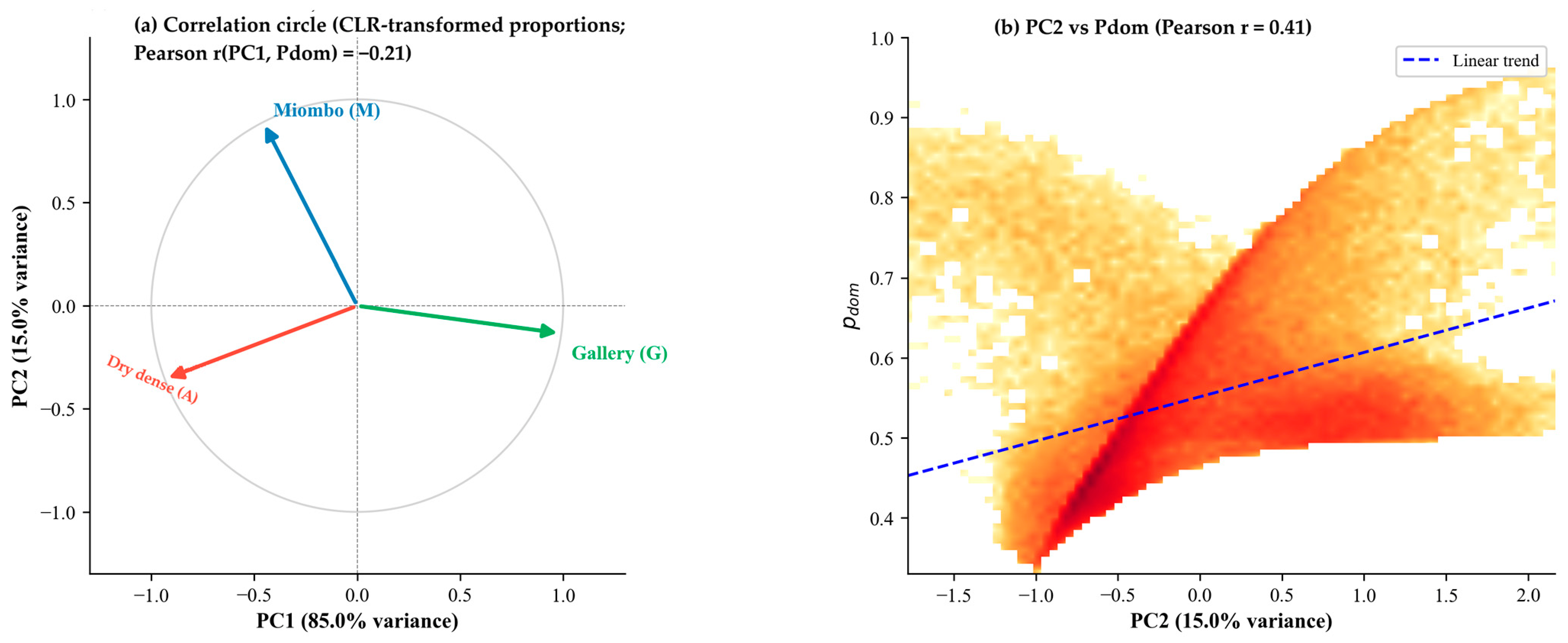
Figure A3.
Panels (a–c). Sensitivity analyses and compositional metric relationships. Panel (a) shows the percentage of forested pixels exceeding each dominance threshold (0.70, 0.75, 0.80). The retained threshold (Pdom > 0.75) yields 7.9% of pixels classified as dominant. The sharp decrease from 12.2% at 0.70 to 4.6% at 0.80 (−7.6 percentage points) identifies 0.75 as an inflection point between overly permissive and overly restrictive classification. Panel (b) shows the distribution of pixels by mixture class (1, 2, or 3 forest types above the softmax presence threshold) across three tested values (3%, 5%, 10%). Two findings hold across the full range: mono-type pixels remain negligible (0.1–1.4%), confirming that near-universal compositional mixing is robust to threshold choice; the two- versus three-type partition varies substantially (47.8–68.2% for two types) and should be read as an order-of-magnitude indicator. Panel (c) shows the density scatter of Pdom versus normalised Shannon entropy H′ (n = 100,000; colour scale: pixel count, log). The dashed curve marks the theoretical maximum H′ for a given Pdom, assuming an equal distribution of residual cover. The strong negative relationship (Pearson r = 0.835; Spearman rs = 0.810) confirms that both metrics describe the same primary gradient of overall mixing intensity from complementary angles. The pixel cloud lying below the theoretical maximum indicates that residual cover concentrates in a single minority type rather than being evenly distributed, consistent with Miombo woodland’s spatial dominance across the province.
References
- Buchhorn, M.; Lesiv, M.; Tsendbazar, N.-E.; Herold, M.; Bertels, L.; Smets, B. Copernicus Global Land Cover Layers—Collection 2. Remote Sens. 2020, 12, 1044. [Google Scholar] [CrossRef] [Scilit]
- Brown, C.F.; Brumby, S.P.; Guzder-Williams, B.; Birch, T.; Hyde, S.B.; Mazzariello, J.; Czerwinski, W.; Pasquarella, V.J.; Haertel, R.; Ilyushchenko, S.; et al. Dynamic World, near real-time global 10 m land use land cover mapping. Sci. Data 2022, 9, 251. [Google Scholar] [CrossRef] [Scilit]
- Useni Sikuzani, Y.; Mpanda Mukenza, M.; Kikuni Tchowa, J.; Kabamb Kanyimb, D.; Malaisse, F.; Bogaert, J. Hierarchical analysis of Miombo woodland spatial dynamics in Lualaba Province (Democratic Republic of the Congo), 1990–2024: Integrating remote sensing and landscape ecology techniques. Remote Sens. 2024, 16, 3903. [Google Scholar] [CrossRef] [Scilit]
- Tyukavina, A.; Hansen, M.C.; Potapov, P.; Parker, D.; Okpa, C.; Stehman, S.V.; Kommareddy, I.; Turubanova, S. Congo basin forest loss dominated by increasing smallholder clearing. Sci. Adv. 2018, 4, eaat2993. [Google Scholar] [CrossRef] [Scilit] [PubMed]
- Picard, J.; Nungi-Pambu Dembi, M.M.; Barbier, N.; Cornu, G.; Couteron, P.; Forni, E.; Gibbon, G.; Lim, F.; Ploton, P.; Pouteau, R.; et al. Combining satellite and field data reveals Congo’s forest types structure, functioning and composition. Remote Sens. Ecol. Conserv. 2025, 11, 200–220. [Google Scholar] [CrossRef] [Scilit]
- Sexton, J.O.; Song, X.-P.; Feng, M.; Noojipady, P.; Anand, A.; Huang, C.; Kim, D.-H.; Collins, K.M.; Channan, S.; DiMiceli, C.; et al. Global, 30-m resolution continuous fields of tree cover. Int. J. Digit. Earth 2013, 6, 427–448. [Google Scholar] [CrossRef] [Scilit]
- Castle, S.E.; Newton, P.; Oldekop, J.A.; Baylis, K.; Miller, D.C. Global forest dataset incongruence creates high uncertainties for conservation, climate, and development policy. One Earth 2026, 9, 101558. [Google Scholar] [CrossRef] [Scilit]
- Bastin, J.-F.; Berrahmouni, N.; Grainger, A.; Maniatis, D.; Mollicone, D.; Moore, R.; Patriarca, C.; Picard, N.; Sparrow, B.; Abraham, E.M. The extent of forest in dryland biomes. Science 2017, 356, 635–638. [Google Scholar] [CrossRef] [Scilit]
- Ryan, C.M.; Williams, M.; Grace, J. Above- and belowground carbon stocks in a miombo woodland landscape of Mozambique. Biotropica 2011, 43, 423–432. [Google Scholar] [CrossRef] [Scilit]
- White, F. The Vegetation of Africa; UNESCO: Paris, France, 1983. [Google Scholar]
- Abdou Amadou, S.; Lawali, D.; Bastin, J.-F.; Bogaert, J.; Michez, A.; Meersmans, J. Effect of Spatial Resolution on Land Cover Mapping in an Agropastoral Area of Niger (Aguié and Mayahi) Using Sentinel-2 and Landsat 8 Imagery Within a Random Forest Regression Framework. Remote Sens. 2026, 18, 750. [Google Scholar] [CrossRef] [Scilit]
- Atkinson, P.M. Resolution manipulation and sub-pixel mapping. In Remote Sensing Image Analysis: Including the Spatial Domain; De Jong, S.M., Van der Meer, F.D., Eds.; Springer: Dordrecht, The Netherlands, 2004; pp. 51–70. [Google Scholar]
- Keshava, N.; Mustard, J.F. Spectral unmixing. IEEE Signal Process. Mag. 2002, 19, 44–57. [Google Scholar] [CrossRef] [Scilit]
- Foody, G.M.; Atkinson, P.M. Uncertainty in Remote Sensing and GIS; Wiley: Chichester, UK, 2002. [Google Scholar] [CrossRef] [Scilit]
- DiMiceli, C.; Carroll, M.; Sohlberg, R.; Kim, D.; Kelly, M.; Townshend, J. MOD44B MODIS/Terra Vegetation Continuous Fields Yearly L3 Global 250m SIN Grid V006; NASA EOSDIS Land Processes DAAC: Sioux Falls, SD, USA, 2015. [CrossRef]
- Hansen, M.C.; Potapov, P.V.; Moore, R.; Hancher, M.; Turubanova, S.A.; Tyukavina, A.; Thau, D.; Stehman, S.V.; Goetz, S.J.; Loveland, T.R.; et al. High-resolution global maps of 21st-century forest cover change. Science 2013, 342, 850–853. [Google Scholar] [CrossRef] [Scilit]
- Belgiu, M.; Drăguț, L. Random forest in remote sensing: A review of applications and future directions. ISPRS J. Photogramm. Remote Sens. 2016, 114, 24–31. [Google Scholar] [CrossRef] [Scilit]
- Reiner, F.; Brandt, M.; Tong, X.; Skole, D.; Kariryaa, A.; Ciais, P.; Davies, A.; Hiernaux, P.; Chave, J.; Mugabowindekwe, M.; et al. More than one quarter of Africa’s tree cover is found outside areas previously classified as forest. Nat. Commun. 2023, 14, 2258. [Google Scholar] [CrossRef] [Scilit]
- Reichstein, M.; Camps-Valls, G.; Stevens, B.; Jung, M.; Denzler, J.; Carvalhais, N.; Prabhat. Deep learning and process understanding for data-driven Earth system science. Nature 2019, 566, 195–204. [Google Scholar] [CrossRef] [Scilit]
- Kattenborn, T.; Leitloff, J.; Schiefer, F.; Hinz, S. Review on convolutional neural networks (CNN) in vegetation remote sensing. ISPRS J. Photogramm. Remote Sens. 2021, 173, 24–49. [Google Scholar] [CrossRef] [Scilit]
- Allred, B.W.; Bestelmeyer, B.T.; Boyd, C.S.; Brown, C.; Davies, K.W.; Duniway, M.C.; Ellsworth, L.M.; Erickson, T.A.; Fuhlendorf, S.D.; Griffiths, T.V.; et al. Improving Landsat predictions of rangeland fractional cover with multitask learning and uncertainty. Methods Ecol. Evol. 2021, 12, 841–849. [Google Scholar] [CrossRef] [Scilit]
- Schug, F.; Pfoch, K.A.; Pham, V.-D.; van der Linden, S.; Okujeni, A.; Frantz, D.; Radeloff, V.C. Land cover fraction mapping across global biomes with Landsat data, spatially generalized regression models and spectral-temporal metrics. Remote Sens. Environ. 2024, 311, 114260. [Google Scholar] [CrossRef] [Scilit]
- Pan, Y.; Birdsey, R.A.; Fang, J.; Houghton, R.; Kauppi, P.E.; Kurz, W.A.; Phillips, O.L.; Shvidenko, A.; Lewis, S.L.; Canadell, J.G.; et al. A large and persistent carbon sink in the world’s forests. Science 2011, 333, 988–993. [Google Scholar] [CrossRef] [Scilit]
- Olander, L.P.; Gibbs, H.K.; Steininger, M.; Swenson, J.J.; Murray, B.C. Reference scenarios for deforestation and forest degradation in support of REDD. Environ. Res. Lett. 2008, 3, 025011. [Google Scholar] [CrossRef] [Scilit]
- Olofsson, P.; Foody, G.M.; Herold, M.; Stehman, S.V.; Woodcock, C.E.; Wulder, M.A. Good practices for estimating area and assessing accuracy of land change. Remote Sens. Environ. 2014, 148, 42–57. [Google Scholar] [CrossRef] [Scilit]
- Colditz, R.R. An evaluation of different training sample allocation schemes for discrete and continuous land cover classification using decision tree-based algorithms. Remote Sens. 2015, 7, 9655–9681. [Google Scholar] [CrossRef] [Scilit]
- Roberts, D.R.; Bahn, V.; Ciuti, S.; Boyce, M.S.; Elith, J.; Guillera-Arroita, G.; Hauenstein, S.; Lahoz-Monfort, J.J.; Schröder, B.; Thuiller, W.; et al. Cross-validation strategies for data with temporal, spatial, hierarchical, or phylogenetic structure. Ecography 2017, 40, 913–929. [Google Scholar] [CrossRef] [Scilit]
- Valavi, R.; Elith, J.; Lahoz-Monfort, J.J.; Guillera-Arroita, G. blockCV: An R package for generating spatially or environmentally separated folds for k-fold cross-validation of species distribution models. Methods Ecol. Evol. 2019, 10, 225–232. [Google Scholar] [CrossRef] [Scilit]
- FAO. Global Forest Resources Assessment 2020: Main Report; Food and Agriculture Organization of the United Nations: Rome, Italy, 2020. [Google Scholar]
- Timberlake, J.; Chidumayo, E.; Sawadogo, L. Distribution and characteristics of African dry forests and woodlands. In The Dry Forests and Woodlands of Africa: Managing for Products and Services; Chidumayo, E.N., Gumbo, D.J., Eds.; Earthscan: London, UK, 2010; pp. 11–42. [Google Scholar]
- Vrieling, A.; Meroni, M.; Darvishzadeh, R.; Skidmore, A.K.; Wang, T.; Zurita-Milla, R.; Oosterbeek, K.; O’Connor, B.; Paganini, M. Vegetation phenology from Sentinel-2 and field cameras for a Dutch barrier island. Remote Sens. Environ. 2018, 215, 517–529. [Google Scholar] [CrossRef] [Scilit]
- Bey, A.; Sánchez-Paus Díaz, A.; Maniatis, D.; Marchi, G.; Mollicone, D.; Ricci, S.; Bastin, J.-F.; Moore, R.; Federici, S.; Rezende, M.; et al. Collect Earth: Land Use and Land Cover Assessment through Augmented Visual Interpretation. Remote Sens. 2016, 8, 807. [Google Scholar] [CrossRef] [Scilit]
- Colditz, R.R.; Schmidt, M.; Conrad, C.; Hansen, M.C.; Dech, S. Land cover classification with coarse spatial resolution data to derive continuous and discrete maps for complex regions. Remote Sens. Environ. 2011, 115, 3264–3275. [Google Scholar] [CrossRef] [Scilit]
- Gorelick, N.; Hancher, M.; Dixon, M.; Ilyushchenko, S.; Thau, D.; Moore, R. Google Earth Engine: Planetary-scale geospatial analysis for everyone. Remote Sens. Environ. 2017, 202, 18–27. [Google Scholar] [CrossRef] [Scilit]
- Hastie, T.; Tibshirani, R.; Friedman, J. The Elements of Statistical Learning: Data Mining, Inference, and Prediction, 2nd ed.; Springer: New York, NY, USA, 2009. [Google Scholar]
- Georganos, S.; Grippa, T.; Vanhuysse, S.; Lennert, M.; Shimoni, M.; Kalogirou, S.; Wolff, E. Less is more: Optimizing classification performance through feature selection in a very-high-resolution remote sensing object-based urban application. GIScience Remote Sens. 2018, 55, 221–242. [Google Scholar] [CrossRef] [Scilit]
- Wright, M.N.; Ziegler, A. ranger: A fast implementation of random forests for high dimensional data in C++ and R. J. Stat. Softw. 2017, 77, 1–17. [Google Scholar] [CrossRef] [Scilit]
- Breiman, L. Random forests. Mach. Learn. 2001, 45, 5–32. [Google Scholar] [CrossRef] [Scilit]
- Probst, P.; Wright, M.N.; Boulesteix, A.-L. Hyperparameters and tuning strategies for random forest. WIREs Data Min. Knowl. Discov. 2019, 9, e1301. [Google Scholar] [CrossRef] [Scilit]
- Aitchison, J. The Statistical Analysis of Compositional Data; Chapman & Hall: London, UK, 1986. [Google Scholar]
- Ioffe, S.; Szegedy, C. Batch normalization: Accelerating deep network training by reducing internal covariate shift. In Proceedings of the 32nd International Conference on Machine Learning (ICML), Lille, France, 6–11 July 2015; pp. 448–456. [Google Scholar]
- Srivastava, N.; Hinton, G.; Krizhevsky, A.; Sutskever, I.; Salakhutdinov, R. Dropout: A simple way to prevent neural networks from overfitting. J. Mach. Learn. Res. 2014, 15, 1929–1958. [Google Scholar]
- Goodfellow, I.; Bengio, Y.; Courville, A. Deep Learning; MIT Press: Cambridge, MA, USA, 2016. [Google Scholar]
- Kingma, D.P.; Ba, J. Adam: A method for stochastic optimization. In Proceedings of the 3rd International Conference on Learning Representations (ICLR), San Diego, CA, USA, 7–9 May 2015. [Google Scholar]
- Willmott, C.J.; Matsuura, K. Advantages of the mean absolute error (MAE) over the root mean square error (RMSE) in assessing average model performance. Clim. Res. 2005, 30, 79–82. [Google Scholar] [CrossRef] [Scilit]
- Foody, G.M. Status of land cover classification accuracy assessment. Remote Sens. Environ. 2002, 80, 185–201. [Google Scholar] [CrossRef] [Scilit]
- Fisher, P.F. The pixel: A snare and a delusion. Int. J. Remote Sens. 1997, 18, 679–685. [Google Scholar] [CrossRef] [Scilit]
- Cracknell, A.P. Synergy in remote sensing—what’s in a pixel? Int. J. Remote Sens. 1998, 19, 2025–2047. [Google Scholar] [CrossRef] [Scilit]
- Fernandes, R.; Fraser, R.; Latifovic, R.; Cihlar, J.; Beaubien, J.; Du, Y. Approaches to fractional land cover and continuous field mapping: A comparative assessment over the BOREAS study region. Remote Sens. Environ. 2004, 89, 234–251. [Google Scholar] [CrossRef] [Scilit]
- Shannon, C.E. A mathematical theory of communication. Bell Syst. Tech. J. 1948, 27, 379–423. [Google Scholar] [CrossRef] [Scilit]
- Pielou, E.C. The measurement of diversity in different types of biological collections. J. Theor. Biol. 1966, 13, 131–144. [Google Scholar] [CrossRef] [Scilit]
- Lluïsà, J.; Ogaya, R.; Sardans, J.; Peñuelas, J. Mapping tree species fractions in temperate mixed forests using Sentinel-2 time series and synthetically mixed training data. Remote Sens. Environ. 2025, 323, 114740. [Google Scholar] [CrossRef] [Scilit]
- Somers, B.; Asner, G.P.; Tits, L.; Coppin, P. Endmember variability in spectral mixture analysis: A review. Remote Sens. Environ. 2011, 115, 1603–1616. [Google Scholar] [CrossRef] [Scilit]
- Zhu, Z.; Zhang, J.; Yang, Z.; Aljaddani, A.H.; Cohen, W.B.; Qiu, S.; Zhou, C. Continuous monitoring of land disturbance based on Landsat time series. Remote Sens. Environ. 2020, 238, 111116. [Google Scholar] [CrossRef] [Scilit]
- Herold, M.; Mayaux, P.; Woodcock, C.E.; Baccini, A.; Schmullius, C. Some challenges in global land cover mapping: An assessment of agreement and accuracy in existing 1 km datasets. Remote Sens. Environ. 2008, 112, 2538–2556. [Google Scholar] [CrossRef] [Scilit]
- Potapov, P.; Hansen, M.C.; Pickens, A.; Hernandez-Serna, A.; Tyukavina, A.; Turubanova, S.; Zalles, V.; Li, X.; Khan, A.; Stolle, F.; et al. The global 2000–2020 land cover and land use change dataset derived from the Landsat archive: The GLC-SHARE dataset. Front. Remote Sens. 2022, 3, 856903. [Google Scholar] [CrossRef] [Scilit]
- Gal, Y.; Ghahramani, Z. Dropout as a Bayesian approximation: Representing model uncertainty in deep learning. In Proceedings of the 33rd International Conference on Machine Learning (ICML), New York, NY, USA, 19–24 June 2016; pp. 1050–1059. [Google Scholar]
- Meyer, H.; Reudenbach, C.; Wollauer, S.; Nauss, T. Importance of spatial predictor variable selection in machine learning applications—Moving from data reproduction to spatial prediction. Ecol. Model. 2018, 411, 108815. [Google Scholar] [CrossRef] [Scilit]
- Wadoux, A.M.J.-C.; Heuvelink, G.B.M.; De Bruin, S.; Brus, D.J. Spatial cross-validation is not the right way to evaluate map accuracy. Ecol. Model. 2021, 457, 109692. [Google Scholar] [CrossRef] [Scilit]
- Réjou-Méchain, M.; Barbier, N.; Couteron, P.; Ploton, P.; Vincent, G.; Herold, M.; Mermoz, S.; Saatchi, S.; Chave, J.; de Boissieu, F.; et al. Upscaling forest biomass from field to satellite measurements: Sources of errors and ways to reduce them. Surv. Geophys. 2019, 40, 881–911. [Google Scholar] [CrossRef] [Scilit]
- Higginbottom, T.P.; Symeonakis, E. Assessing land degradation and desertification using vegetation index data: Current frameworks and future directions. Remote Sens. 2014, 6, 9552–9575. [Google Scholar] [CrossRef] [Scilit]
- Grantham, H.S.; Duncan, A.; Evans, T.D.; Jones, K.R.; Beyer, H.L.; Schuster, R.; Walston, J.; Ray, J.C.; Robinson, J.G.; Callow, M.; et al. Anthropogenic modification of forests means only 40% of remaining forests have high ecosystem integrity. Nat. Commun. 2020, 11, 5978. [Google Scholar] [CrossRef] [Scilit]
- Wan, L.; Ciais, P.; de Truchis, A.; Sean, E.; Fischer, F.J.; Purnell, D.; Ploton, P. Satellite-based mapping of annual canopy height and aboveground biomass in African dense forests. Front. Remote Sens. 2025, 6, 1724950. [Google Scholar] [CrossRef] [Scilit]
- Duncanson, L.; Kellner, J.R.; Armston, J.; Dubayah, R.; Minor, D.M.; Hancock, S.; Healey, S.P.; Patterson, P.L.; Saarela, S.; Marselis, S.; et al. Aboveground biomass density models for NASA’s Global Ecosystem Dynamics Investigation (GEDI) lidar mission. Remote Sens. Environ. 2022, 270, 112845. [Google Scholar] [CrossRef] [Scilit]
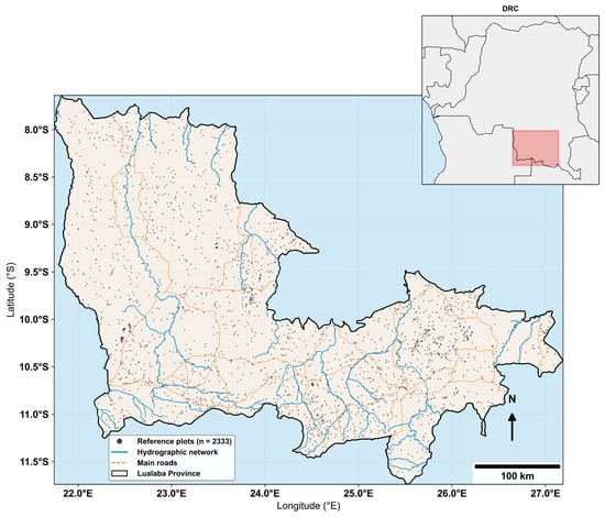
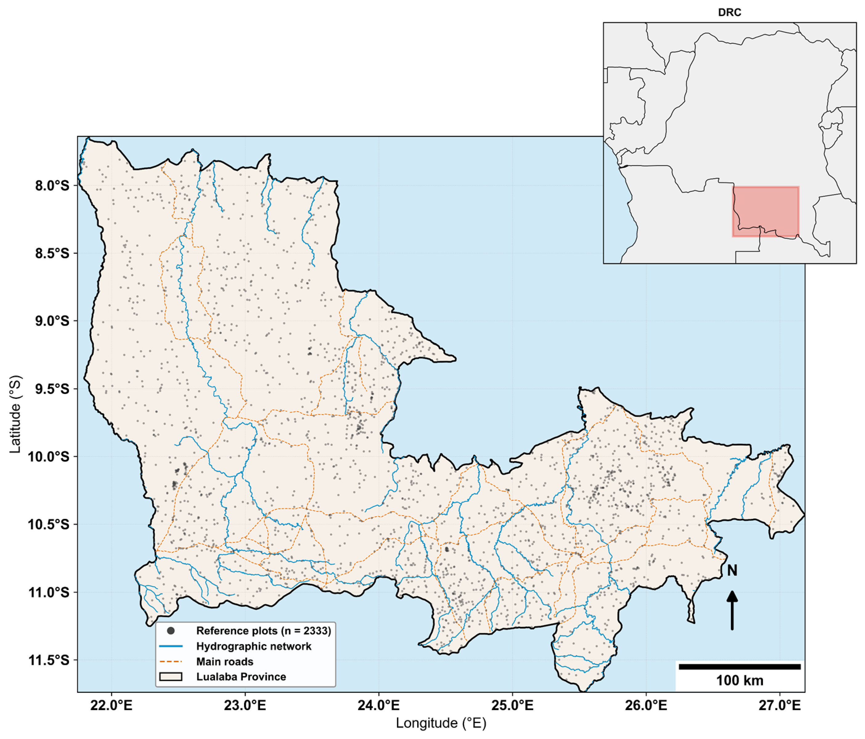
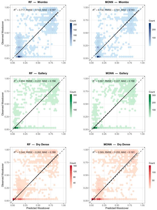
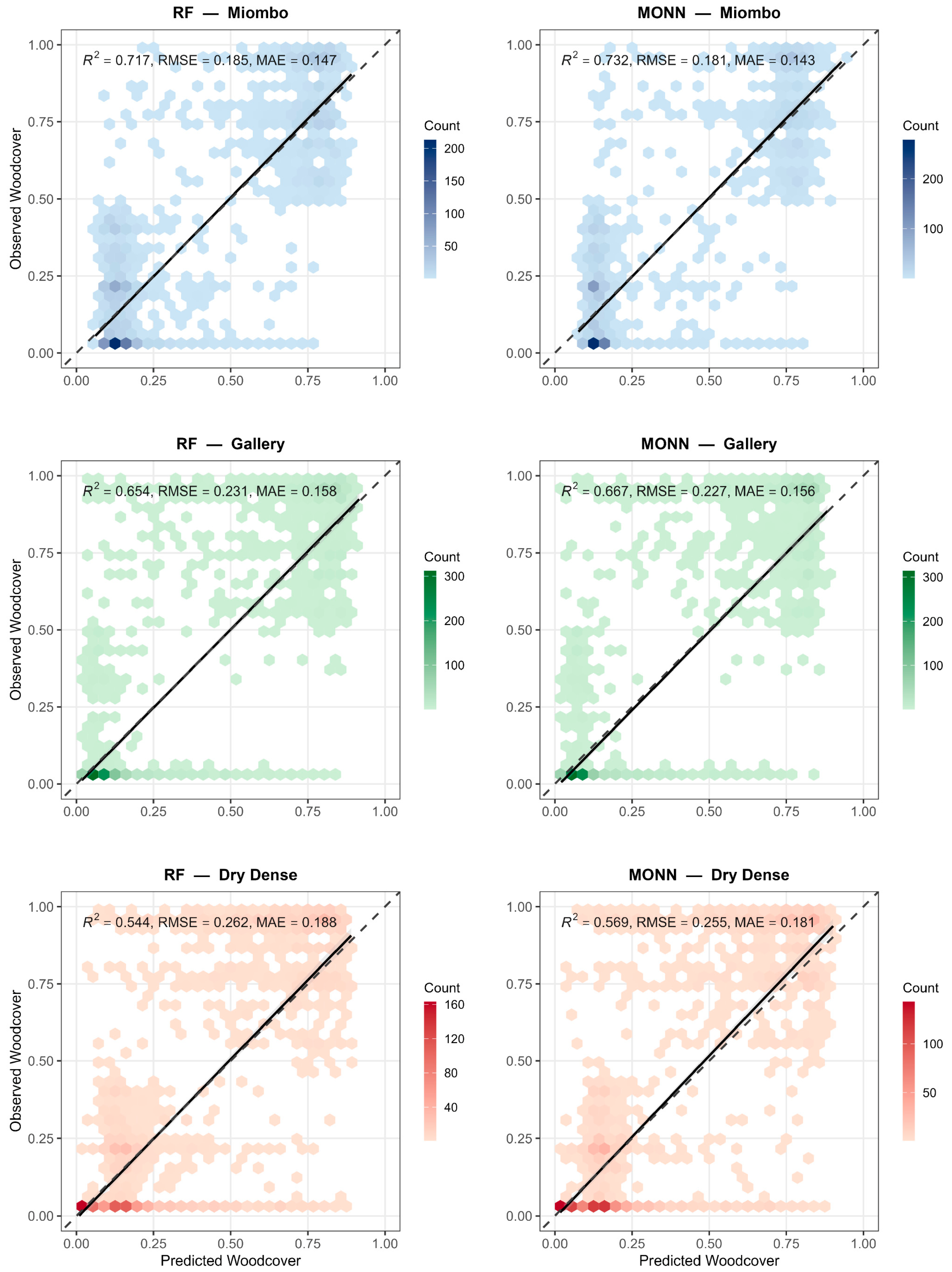
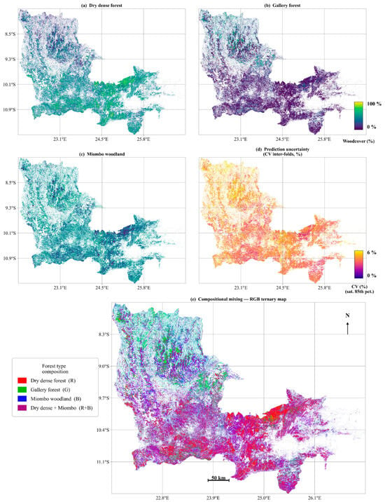
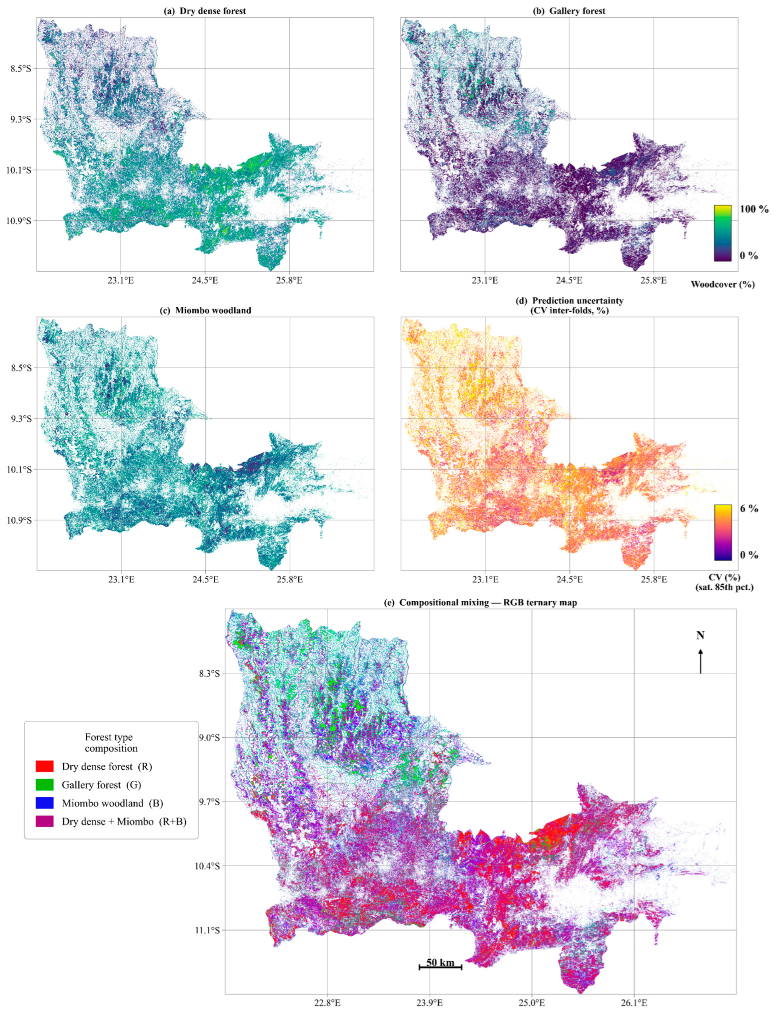
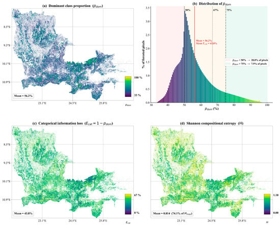
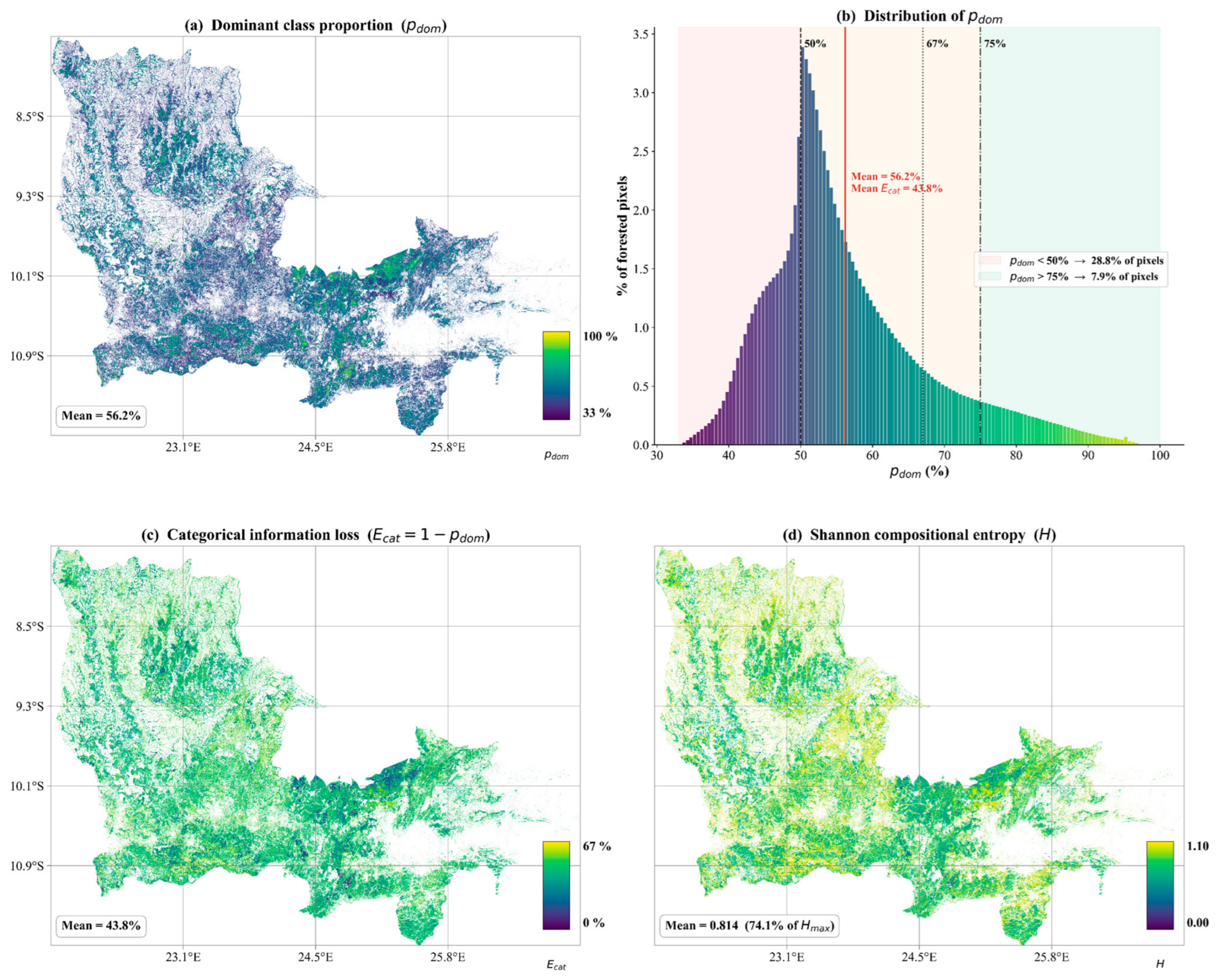
Disclaimer/Publisher’s Note: The statements, opinions and data contained in all publications are solely those of the individual author(s) and contributor(s) and not of MDPI and/or the editor(s). MDPI and/or the editor(s) disclaim responsibility for any injury to people or property resulting from any ideas, methods, instructions or products referred to in the content. |
© 2026 by the authors. Licensee MDPI, Basel, Switzerland. This article is an open access article distributed under the terms and conditions of the Creative Commons Attribution (CC BY) license.