Article

Stage-Specific Estimation of Maize Flavonoids Using UAV Multispectral Imagery and Spectral, Texture, and Phenological Features

1
College of Natural Resources and Environment, Northwest A&F University, Yangling 712100, China
2
Institute of Farmland Irrigation, Chinese Academy of Agricultural Sciences, Xinxiang 453002, China
3
Baoji Agricultural Technology Extension Service Center, Baoji 721000, China
*
Author to whom correspondence should be addressed.
Remote Sens. 2026, 18(12), 1978; https://doi.org/10.3390/rs18121978
Submission received: 17 April 2026 / Revised: 10 June 2026 / Accepted: 12 June 2026 / Published: 14 June 2026
(This article belongs to the Special Issue Perspectives of Remote Sensing for Precision Agriculture)

Highlights

What are the main findings?
  • Multisource feature fusion substantially improves UAV-based estimation of maize flavonoid content.
  • The optimal feature–model combination varies across maize growth stages, with texture and phenological descriptors providing important complementary information.
What are the implications of the main findings?
  • Maize flavonoids can be monitored non-destructively at canopy scale using UAV multispectral imagery.
  • Combining spatial and temporal information improves the consistency and reliability of biochemical trait assessment in field conditions.

Abstract

Rapid and non-destructive estimation of maize (Zea mays L.) leaf flavonoid (Flav) content is important for crop stress monitoring and precision agriculture. This study aimed to improve Flav estimation by integrating unmanned aerial vehicle (UAV)-based multispectral data, texture features, and phenological parameters across six key growth stages in the Guanzhong Plain, China. Maize Flav content was measured in situ using a Dualex Scientific+ meter, while canopy reflectance was acquired with a DJI M300 RTK UAV equipped with an MS600 Pro multispectral camera. A comprehensive feature set, including spectral bands, vegetation indices, texture features, texture indices, and logistic curve-derived phenological parameters, was constructed. Three feature selection methods, competitive adaptive reweighted sampling (CARS), the genetic algorithm (GA), and the successive projections algorithm (SPA), together with three regression models, partial least squares regression (PLSR), extreme gradient boosting (XGBoost), and convolutional neural network (CNN), were evaluated for Flav estimation. The results showed that integrating spectral, texture, and phenological information significantly improved model performance compared with spectral variables alone. CNN and XGBoost generally outperformed PLSR. Across the six growth stages, the stage-specific optimal models achieved coefficient of determination (R2) values ranging from 0.7749 to 0.8686 and residual prediction deviation (RPD) values ranging from 2.0046 to 2.6019, indicating high to outstanding predictive ability. The highest accuracy was obtained at R3 using the CARS-XII-CNN model, with R2 = 0.8686, root mean square error of validation (RMSEV) = 0.0382, and RPD = 2.6019. Texture features and phenological metrics, especially the start of season derived from the normalized difference vegetation index (NDVI_SOS) and the rate of senescence derived from the enhanced vegetation index (EVI_ROS), contributed substantially to model accuracy. In addition, maize Flav showed a unimodal response to nitrogen supply, with moderate nitrogen levels associated with higher Flav content. This study demonstrates the potential of UAV-based multisource feature integration and machine learning for accurate maize Flav estimation, and provides a useful framework for digital crop phenotyping and stress diagnosis.

1. Introduction

Maize (Zea mays L.) is one of the most important food crops worldwide and plays a crucial role in ensuring food security [1,2,3,4]. Under the increasing pressures of climate change and frequent extreme weather events, rapid and accurate monitoring of maize growth status has become essential for stress diagnosis and precision crop management. In this context, unmanned aerial vehicle (UAV)-based multispectral remote sensing has become an important tool in agricultural monitoring because it provides flexible, high-throughput, and relatively low-cost observations at critical growth stages [5,6,7,8,9]. Compared with satellite and ground-based sensing platforms, UAV multispectral systems can efficiently capture canopy reflectance in visible, near-infrared, and red-edge bands with high spatial and temporal resolution, making them particularly suitable for field-scale crop phenotyping and agronomic parameter estimation.
To date, UAV multispectral data have been widely used to estimate crop biophysical and biochemical traits, including chlorophyll content, nitrogen nutrition status, leaf area index, biomass, water stress, and yield [10,11]. These studies demonstrate the effectiveness of UAV multispectral imagery for crop trait estimation, but most of them have focused on primary growth- or photosynthesis-related traits rather than secondary metabolites such as flavonoids. Previous studies have shown that integrating spectral information with texture or temporal features can improve model robustness and predictive performance by providing complementary information on canopy reflectance, spatial heterogeneity, and crop developmental dynamics [12,13,14,15,16,17]. This provides a methodological basis for using multisource feature fusion to estimate crop traits that are influenced by both physiological status and canopy structure. Texture descriptors derived from high-resolution imagery can better characterize canopy heterogeneity, while phenological information extracted from vegetation index time series can capture crop developmental dynamics that are difficult to represent using single-date spectral features alone. These advances indicate that multisource feature integration may provide a more effective strategy for assessing crop traits than relying solely on reflectance or vegetation indices. However, studies on flavonoids (Flav) remain relatively limited, especially at the maize canopy scale. Therefore, it remains unclear whether multisource feature fusion strategies developed for common crop traits can be effectively applied to UAV-based estimation of maize flavonoids.
Flavonoids are important secondary metabolites involved in plant responses to environmental stress, including excess radiation, drought, and biotic stress [18,19,20,21,22,23]. In maize, flavonoids are closely related to physiological resistance and stress adaptation, and their rapid and non-destructive estimation can therefore provide valuable information for crop stress monitoring and growth evaluation. Traditionally, plant flavonoids are quantified using solvent extraction followed by spectrophotometric or chromatographic analysis, which is destructive, time-consuming, and unsuitable for high-throughput field monitoring. The Dualex Scientific+ meter provides a rapid and non-destructive optical measurement of leaf epidermal flavonoid-related signals. Unlike chemical assays that directly quantify total flavonoid concentration, the Flav output of Dualex is derived from the epidermal screening of chlorophyll fluorescence under ultraviolet and reference excitation conditions. Therefore, it represents an optical proxy of epidermal flavonoids, mainly flavonols, rather than a direct chemical measurement of total flavonoid concentration. The Dualex technical documentation defines Flv as an index of phenolics, mostly flavonols, and recent user documentation further describes Flav as a flavonol index measured by the Dualex leaf-clip sensor [24]. Previous validation studies have also supported the use of Dualex for non-destructive assessment of leaf polyphenolic compounds and epidermal flavonoid-related signals [25,26]. Accordingly, Dualex-based Flav readings provide a practical basis for field-scale monitoring of leaf flavonoid-related variation. In the present study, this Dualex-derived Flav value was used as the response variable, allowing UAV multispectral features to be linked with non-destructive ground measurements of epidermal flavonoid signals.
Phenology is another critical factor affecting crop spectral responses and trait retrieval [27,28,29]. Crop growth stages regulate canopy structure, pigment accumulation, and physiological activity, which in turn influence the relationship between reflectance signals and target traits. Incorporating phenological metrics may therefore help models better capture stage-dependent variation and improve their interpretability across growth stages. This is particularly relevant for maize Flav estimation because flavonoid accumulation and canopy reflectance both vary with growth stage and stress conditions. Despite this potential, the combined contribution of spectral, texture, and phenological features to maize Flav estimation has not been systematically evaluated. In addition, although feature selection methods such as competitive adaptive reweighted sampling (CARS), the genetic algorithm (GA), and the successive projections algorithm (SPA) are increasingly used in agricultural remote sensing, their comparative effectiveness for identifying Flav-sensitive spectral, texture, and phenological variables remains unclear. Deep learning approaches, particularly convolutional neural networks (CNNs), may further enhance nonlinear feature extraction, but their suitability for this specific task has not yet been fully investigated [30,31,32].
To address these gaps, this study focused on summer maize in the Guanzhong Plain of China [33,34] and developed a stage-specific UAV-based framework for maize Flav estimation across six key growth stages. Compared with previous UAV-based studies that mainly focused on chlorophyll, nitrogen status, leaf area index, biomass, water stress, or yield estimation [10,11], the main contribution of this study lies in extending UAV multispectral remote sensing to Dualex-based maize Flav estimation and integrating spectral, texture, and phenological descriptors into a unified multisource feature system. This design enables maize Flav variation to be characterized from three complementary perspectives: canopy spectral response, spatial structural heterogeneity, and temporal developmental status. Specifically, the objectives were to: (1) construct a multisource feature set integrating spectral variables, texture descriptors, and phenological parameters; (2) compare the effects of different feature selection strategies and regression models on maize Flav estimation; and (3) identify the optimal stage-specific feature–model combinations for rapid and non-destructive monitoring of maize canopy Flav. This study is expected to provide methodological support for digital crop phenotyping, stress diagnosis, and precision agricultural management.

2. Data and Methodology

2.1. Experimental Design

The experiment was carried out in Qinan Village, Liangshan Town, Qian County, Xianyang, Shaanxi Province, China (108°07′E, 34°38′N; Figure 1), located in the north–central Guanzhong Plain. This region has a warm temperate, semi-humid continental monsoon climate, with a mean annual temperature of 13.1 °C, a frost-free period of 224 days, and annual precipitation ranging from 573 to 590 mm. The site is situated on loess tableland with loessial (Huangmian) soil, and the dominant cropping system is winter wheat–summer maize rotation.
The site has served as a long-term platform for maize monitoring, with 12 consecutive years of field observations under a consistent experimental layout. In 2024, the experiment was conducted from April to August using the maize hybrid Zhengdan 958. Maize was sown on 20 April in 40 plots, each covering 30 m2. Two sampling points were arranged along the diagonal of each plot, giving a total of 80 sampling points (Figure 1c).
The fertilizer treatment layout is shown in Figure 1d. To create nutrient-induced variation in maize growth [35], a three-factor fertilizer experiment was implemented. Nitrogen was applied at five levels (50, 100, 150, 200, and 250 kg ha−1), while phosphorus and potassium were each applied at two levels (0 or 90 kg ha−1 P2O5 and 0 or 75 kg ha−1 K2O, respectively). With two replicates, the experiment resulted in 40 plots. All fertilizers were applied once before sowing as basal fertilizer, and no topdressing was added during the growing season.
The experimental layout followed the fixed design of the long-term maize monitoring field. Although the layout was not fully randomized, the field was located on a relatively flat and homogeneous loess tableland. All plots used the same maize variety, sowing date, planting density, row spacing, and plant spacing. Except for the designed fertilization treatments, all other field management practices were kept consistent and followed local agronomic recommendations. These conditions helped reduce the potential influence of soil and management heterogeneity on UAV-based Flav estimation.
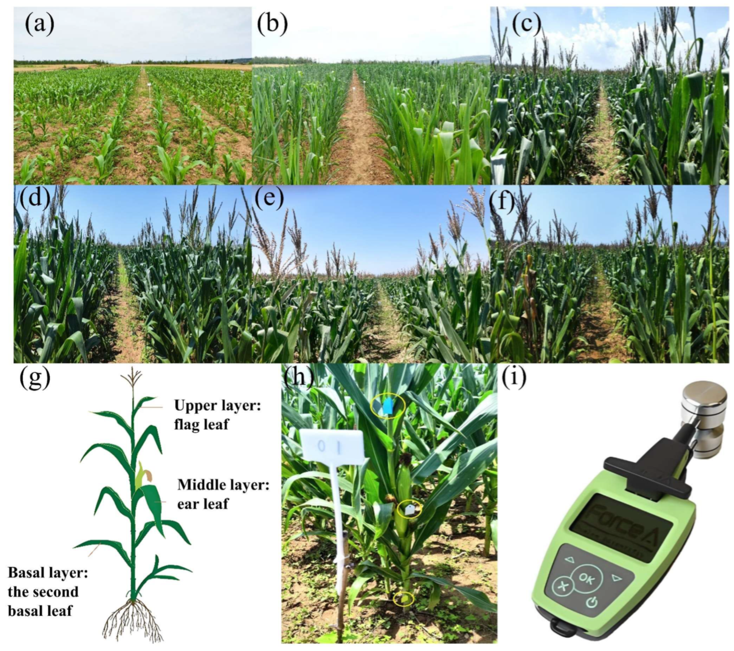
Sampling was conducted at six key growth stages: V6 (11 June, six-leaf stage), V10 (28 June, ten-leaf stage), VT (25 July, tasseling stage), R1 (1 August, silking stage), R2 (13 August, blister stage), and R3 (23 August, milk stage) (Figure 2). At each stage, leaf flavonoid (Flav) content was measured and UAV multispectral imagery was collected.

2.2. Determination of Flavonoid Content in Maize Leaves

To maintain consistency with the measurement principle of the instrument, the response variable used in this study was defined as the Dualex Scientific+ flavonoid proxy, hereafter referred to as Flav. Flav was measured using a Dualex Scientific+ polyphenol chlorophyll meter (Force A, Orsay, France) (Figure 2i), which measures optical signals from a 5 mm2 area of the leaf surface. The instrument estimates compounds related to epidermal flavonoids, mainly flavonols, from the differential screening of chlorophyll fluorescence under ultraviolet and reference excitation conditions, rather than through chemical extraction of total flavonoids [24]. Chlorophyll is estimated from the transmittance ratio between the far-red and near-infrared regions, whereas signals related to flavonoids and anthocyanins are derived from differences in epidermal screening of near-infrared chlorophyll fluorescence under alternating excitation conditions. The Nitrogen Balance Index (NBI) is calculated as Chl/Flav. The descriptions of Chl, Anth, and NBI are provided only to clarify the measurement principle of the instrument; only the Dualex Scientific+ Flav proxy was used as the target variable for model development and retrieval analysis in this study.
At each sampling point (Figure 2h), one representative leaf was selected for measurement at each growth stage. Measurements were taken twice at the leaf tip, middle, and base while avoiding the main veins, and the average value was used as the final Flav content of that sample. A total of 80 Flav samples were obtained at each growth stage.

2.3. Acquisition of Near-Surface UAV Multispectral Data

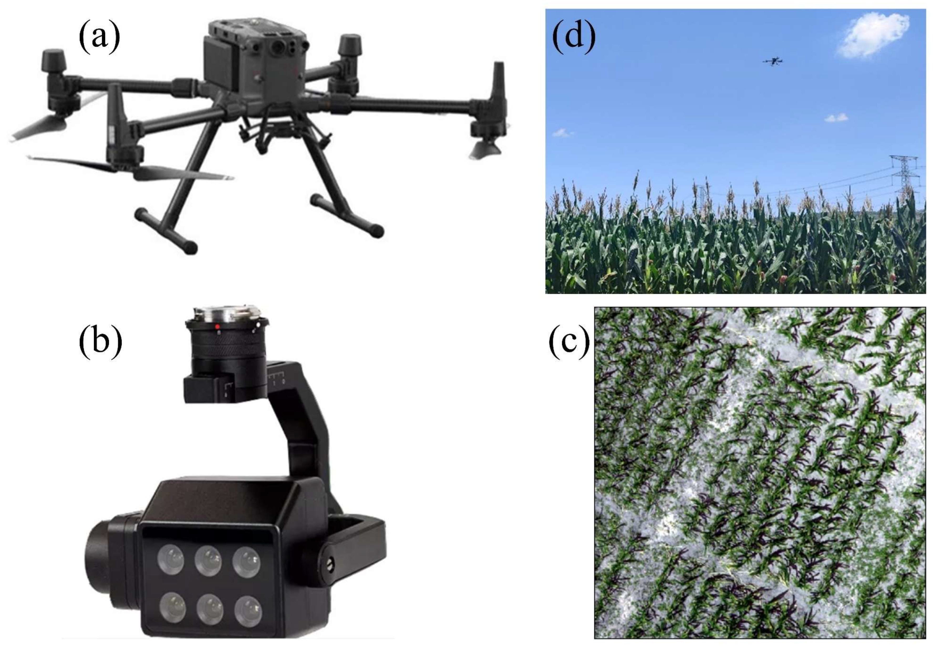
Near-surface imagery in this study was acquired using a DJI M300 RTK unmanned aerial vehicle (SZ DJI Technology Co., Ltd., Shenzhen, China) equipped with an MS600 Pro fixed-band multispectral camera (Yusense Information Technology and Equipment Co., Ltd., Qingdao, China), with six bands centered at 450, 555, 660, 720, 750, and 840 nm, as shown in Figure 3. Prior to each flight, a mission plan and parameters were established: altitude of 20 m, longitudinal overlap of 80%, lateral overlap of 70%, and image ground sampling distance (GSD) of approximately 2 cm. Flights were conducted on calm, cloud-free days between 11:00 and 14:00 local time.
Before each UAV flight, three images of a standard reflectance calibration panel supplied with the MS600 Pro multispectral camera system were collected under the same illumination conditions as the flight mission. If the flight duration exceeded approximately 0.5 h, another three panel images were acquired after landing to account for possible changes in illumination conditions. In Yusense Map, these panel images were used as reference images for radiometric calibration. The known reflectance information of the calibration panel was used to derive band-specific calibration information and convert the raw digital numbers of each multispectral band into reflectance values. After radiometric correction, Yusense Map was used for band registration and image mosaicking. The calibrated multispectral images were then imported into ENVI 5.3, and regions of interest were delineated in areas with uniform maize growth while avoiding bare soil and weeds as much as possible. The mean spectral reflectance of each ROI was extracted as the reflectance value for the corresponding sample point. A total of 480 sample reflectance records were obtained across the six growth stages.

2.4. Multisource Predictor Selection

The candidate predictors included six UAV multispectral bands, conventional vegetation indices, optimized two-band vegetation indices, GLCM-based texture metrics, optimized texture indices, and NDVI- and EVI-derived phenological parameters. These variables were used to construct stage-specific models for maize Flav estimation. To reduce redundancy and identify effective predictor combinations, three feature selection algorithms, including competitive adaptive reweighted sampling (CARS), the genetic algorithm (GA), and the successive projections algorithm (SPA) [36,37,38], were applied to the candidate predictor sets.
CARS, founded on the “survival of the fittest” principle, employs an adaptive weighted-sampling strategy to identify strongly correlated spectral bands [39]. By integrating Monte Carlo sampling with a partial least squares (PLS) model, CARS ranks band importance based on the absolute values of regression coefficients and iteratively adjusts weights, retaining high-contribution bands while discarding redundant ones. Its primary strength lies in efficiently handling high-dimensional data, significantly reducing dimensionality, and enhancing predictive accuracy [40].
GA is a stochastic global search optimizer for high-dimensional spaces, comprising four components: encoding, a fitness function, genetic operators, and run parameters. Mimicking biological evolution, GA performs variable selection through coding, population initialization, selection, crossover, and mutation [41]. With strong global optimization capability, GA tallies the most frequently selected variables across runs, ensuring a consistent variable count. In this study, we set a population size of 50, a 50% crossover rate, a 1% mutation rate, and 100 generations, and pooled the outputs from 100 independent GA runs as model inputs [42].
SPA is a forward selection loop that uses projection operations to choose band sets with minimal collinearity, minimizing redundancy among the selected features [43]. Due to its simplicity and high speed, SPA is ideal for rapid dimensionality reduction, where interpretability is essential. In spectral analysis, SPA continues to reduce redundancy and improve model accuracy, particularly with high-dimensional datasets [44,45].

2.5. Construction of Vegetation Indices

Vegetation indices are strongly associated with plant growth status and foliar physicochemical traits [46,47,48]. By mathematically combining reflectance values from specific spectral bands, these indices mitigate sensor-related and environmental noise, enhance the signal from the target, and improve the efficiency of spectral information, thereby achieving effective dimensionality reduction. In this study, ten commonly used vegetation indices were selected as predictor variables. Their formulas and references are provided in Table 1.
Additionally, identifying the most suitable vegetation index is essential. Therefore, this study further computed optimized spectral indices for every possible two-band combination of the UAV multispectral bands, specifically the optimized difference vegetation index (DVI), optimized normalized difference vegetation index (NDVI), and optimized ratio vegetation index (RVI) (Table 2).

2.6. Texture Feature Extraction

Image texture features describe spatial structure by characterizing gray-level variations within local pixel neighborhoods and can be used to represent surface texture and the spatial distribution patterns of land targets [55]. Principal component analysis (PCA) is a commonly used dimensionality reduction method that transforms high-dimensional data into a smaller set of linearly independent components while retaining the main information of the original dataset [56]. Considering the inter-band correlation and redundancy in UAV multispectral imagery, PCA was first applied to the six-band UAV data to extract the dominant spectral information. The first principal component, which explained the largest proportion of image variance and represented the main canopy reflectance information, was then used as the input image for gray-level co-occurrence matrix (GLCM) texture extraction [57]. Eight GLCM texture metrics, namely mean, variance, homogeneity, contrast, dissimilarity, entropy, second moment, and correlation, were calculated using a 3 × 3 moving window. This window size was selected according to the spatial resolution of the UAV imagery and the fine-scale structural characteristics of the maize canopy.
Additionally, each pair of texture metrics was combined to generate three types of texture indices: the normalized difference texture index (NDTI), the ratio texture index (RTI), and the difference texture index (DTI), as presented in Table 3.

2.7. Phenological Parameter Extraction

Phenology describes the cyclical patterns of plant growth and development and is widely used to characterize crop developmental dynamics and environmental responses. However, the use of phenology-related information for canopy-scale estimation of maize Flav has rarely been explored. In this study, NDVI- and EVI-derived variables were used as temporal-context descriptors rather than fully validated phenological metrics based on dense time-series observations.
For each sampling point, NDVI and EVI values from six UAV acquisition dates were fitted using an S-shaped logistic function, with day of year as the independent variable and NDVI or EVI as the dependent variable. This fitting procedure was intended to describe the relative temporal trajectory of canopy greenness during the monitored maize growth period. To reduce boundary effects, measurements from the V6 and R3 stages were repeated at the two ends of the temporal sequence. This approach was used only as a practical curve-fitting procedure and did not create additional independent observations. Following Zhang et al. [58], the logistic function in Equation (1) was applied to fit the NDVI and EVI trajectories. Four temporal descriptors, SOS, EOS, ROG, and ROS, were derived from the fitted curves and used as candidate predictors for maize Flav estimation. Because only six UAV acquisition dates were available, these descriptors should be interpreted as simplified temporal-context variables.
f ( t ) = a 1 + a 2 1 + e θ 1 ( t β 1 ) a 3 1 + e θ 2 ( t β 2 )
In the equation, a1 represents the baseline level of vegetation activity outside the growing season; a2 and a3 control the amplitudes of change in vegetation growth and senescence, respectively; θ1 and θ2 determine the rates of growth and decline; and β1 and β2 correspond to the pivotal time points (inflection points) on the growth curve.
Based on Equation (1), four phenological metrics were derived: start of season (SOS), end of season (EOS), rate of green-up (ROG), and rate of senescence (ROS), which denote the onset and termination of the vegetation life cycle, as well as the phases of vigor and decline, respectively [59].
The extracted phenological metrics were not used as target variables, but as temporal-context predictors describing maize developmental status at each sampling date. Specifically, NDVI_SOS, NDVI_EOS, NDVI_ROG, NDVI_ROS, EVI_SOS, EVI_EOS, EVI_ROG, and EVI_ROS were combined with spectral and texture variables to form predictor set XIII. These phenological variables were then subjected to the same feature selection procedures, including CARS, GA, and SPA, and were subsequently used together with the selected spectral and texture variables in the PLSR, XGBoost, and CNN models. Thus, phenological information contributed to Flav estimation by providing temporal developmental cues that could not be fully represented by single-date spectral or texture features.

2.8. Model Construction and Accuracy Assessment

The estimation workflow was developed as a stage-specific modeling framework. For each growth stage, Dualex-measured Flav was used as the response variable, while UAV-derived features served as predictors. The Flav values were first ranked in ascending order, followed by stratified random sampling at a 75%:25% ratio to generate the modeling set and the independent test set.
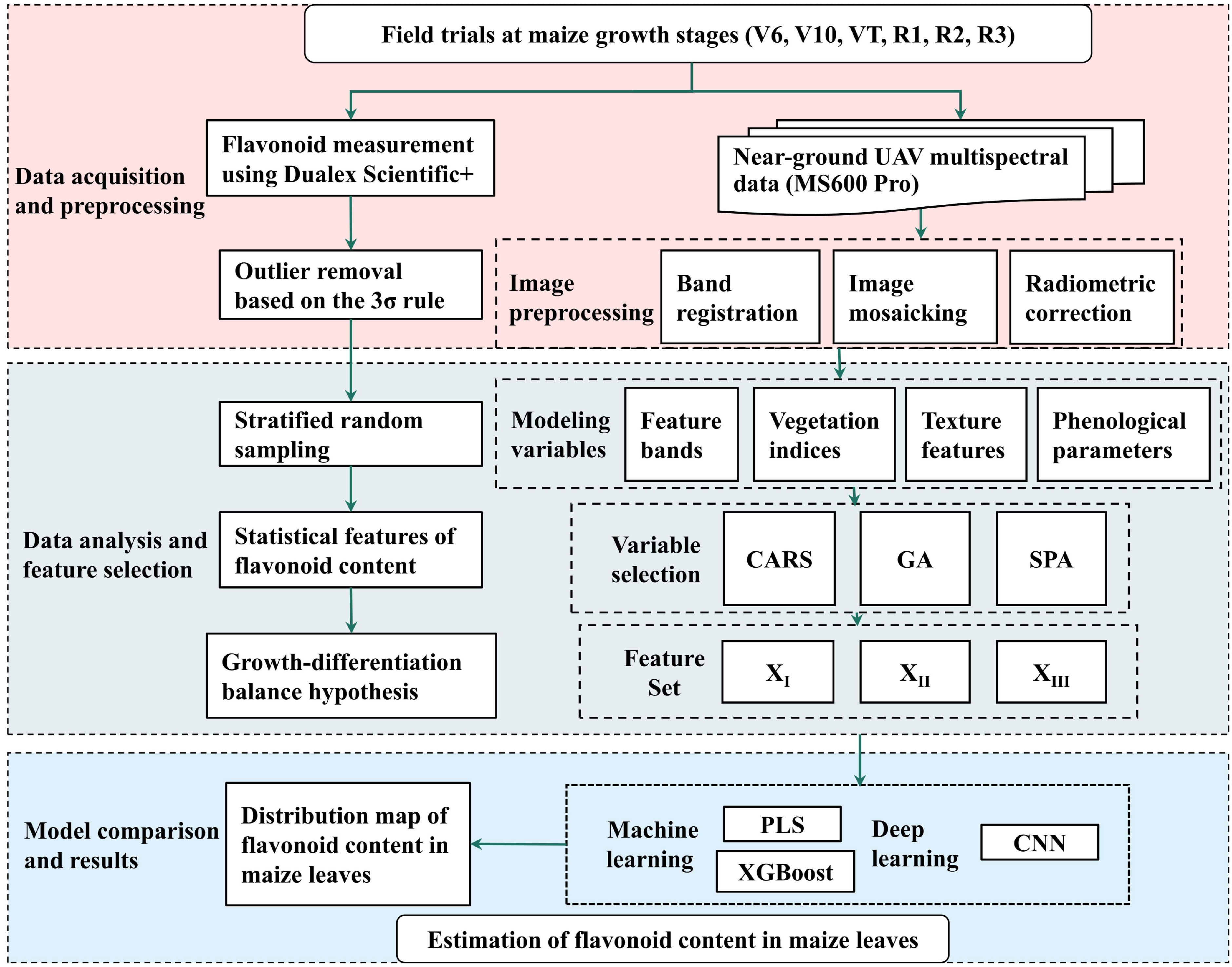
To assess the added value of different feature sources, three predictor sets were constructed. Set XI consisted of single bands, conventional vegetation indices, and optimized vegetation indices. Set XII further included texture features and optimized texture indices. Set XIII incorporated NDVI/EVI-derived temporal growth descriptors in addition to the variables in set XII. Each predictor set was processed using three feature selection methods, including competitive adaptive reweighted sampling (CARS), the genetic algorithm (GA), and the successive projections algorithm (SPA). The selected variables were then used to develop three regression models, namely partial least squares regression (PLSR), extreme gradient boosting regression (XGBoost), and a lightweight convolutional neural network (CNN). All models were trained and evaluated using the same data partitioning strategy. The optimal combination of feature selection method and regression model was determined separately for each growth stage based on R2, RMSEV, and RPD. The overall workflow is shown in Figure 4.
PLSR is a multivariate statistical technique well suited for high-dimensional data and offers significant advantages when severe multicollinearity exists among predictors or when sample sizes are small [60]. By jointly decomposing the predictor and response matrices, PLSR extracts latent variables that capture the maximum covariance between predictors and response variables, and uses them to build a predictive model [61]. PLSR was used to handle high-dimensional spectral, texture, and phenological features with multicollinearity, and input variables were standardized before model fitting; the key model hyperparameter was the number of latent variables. In this study, Bayesian optimization was performed for 30 iterations, and the number of components was selected by minimizing the cross-validation root mean square error.
XGBoost is a scalable, parallelizable, and highly efficient machine learning method that improves upon conventional gradient-boosted decision trees (GBDTs) [62]. XGBoost performs nonlinear fitting by integrating multiple decision trees. During training, regularization terms were applied to control model complexity [63]. The main tuned hyperparameters included the number of trees (n_estimators), maximum tree depth (max_depth), learning rate (learning_rate), subsample ratio (subsample), and column sampling ratio (colsample_bytree). In this study, cross-validation was used to initially set max_depth = 3, min_child_weight = 2, subsample = 0.8, and colsample_bytree = 0.8. Other parameters were left at their default values and were fine-tuned as needed based on model performance.
Convolutional neural networks (CNNs), as a prototypical deep learning architecture, are widely applied in data analytics due to their distinctive structural advantages [64]. Their local receptive fields capture fine-scale features efficiently, while weight sharing keeps parameter counts manageable and computational costs low. Beyond 2-D imagery, CNNs have also proven effective for one-dimensional (1-D) sequential or tabular feature data because of their sensitivity to local patterns and nonlinear feature interactions [65]. To learn nonlinear relationships among the selected multisource variables, this study constructed a lightweight CNN regression model.
Because the input variables in this study were selected spectral, texture, and phenological features rather than raw UAV images, the network was designed as a shallow lightweight architecture to avoid excessive model complexity. The input layer size was [p, 1, 1], where p denotes the number of input features. The backbone comprised two two-dimensional convolutional layers with a kernel size of 3 × 3, 16 filters, the same padding, and default stride. The 3 × 3 kernel was selected because it can capture local combinations among adjacent variables in the reshaped feature space while keeping the number of trainable parameters relatively small. Considering the limited sample size at each growth stage, only two convolutional layers were used to reduce the risk of overfitting while still allowing the network to extract hierarchical nonlinear feature representations.
Each convolutional layer was followed by a rectified linear unit (ReLU) activation layer, and a dropout layer with a dropout rate of 0.1 was used to improve generalization. After flattening, the extracted convolutional features were passed to three fully connected layers with 384, 384, and 1 neurons, respectively, and the final Flav prediction was generated by the regression output layer. The network included two pooling layers to reduce feature dimensionality and improve training stability. Model training used the Adam optimizer, with a maximum of 20 epochs, a mini-batch size of 16, and an initial learning rate of 0.005. These hyperparameters were determined through preliminary trials by balancing model complexity, convergence stability, and validation performance. Performance was monitored on a validation set during training.
All data processing and visualization were conducted using ENVI 5.3, ArcGIS 10.6, MATLAB R2023a, and Python 3.9 within an Anaconda environment.

2.9. Accuracy Assessment

This study used the coefficient of determination (R2), the root mean square error of validation (RMSEV), and the residual prediction deviation (RPD) to evaluate the accuracy of the maize Flav estimation models. Model stability was assessed using five-fold cross-validation. RPD was defined as the ratio of the sample standard deviation (SD) to RMSEV. According to Viscarra Rossel et al. [66], models with RPD < 1.4 are considered non-predictive, 1.4 ≤ RPD < 1.8 allow only coarse estimates, 1.8 ≤ RPD < 2.0 provide reasonable predictions, 2.0 ≤ RPD < 2.5 indicate high accuracy, and RPD > 2.5 indicate outstanding predictive power. In this work, a high-quality Flav model is defined as one with a high R2, a low RMSEV, and, critically, an RPD greater than 2. The formulae are omitted, as these indices are standard in the literature.

3. Results

3.1. Statistical Analysis of Maize Leaf Flavonoids

In total, 1434 leaf-level measurements of maize Flav concentration (Figure 2h) were collected across six key phenological stages, including V6, V10, VT, R1, R2, and R3. Summary statistics for each stage are presented in Table 4, which reveal significant differences in Flav concentration among both growth stages and canopy layers.
Stage-wise trends followed a “low–high–low” pattern. During the vegetative phases (V6 → VT), mean Flav concentration declined steadily from 1.4824 µg cm−2 (V6) to 1.2137 µg cm−2 (VT), with the steepest drop occurring between V6 and V10. In the reproductive phases (R1 → R3) a further, though milder, decrease was observed—from 1.3033 µg cm−2 (R1) to 1.2319 µg cm−2 (R3). Vertically, mean Flav followed the order upper < middle < lower canopy, with statistically significant differences among layers. Except at R3 (where flag-leaf and ear-leaf values converged), the penultimate leaf from the base consistently showed the highest Flav, whereas the flag leaf recorded the lowest. Extremes ranged from 1.6311 µg cm−2 (penultimate leaf, V6) to 0.9541 µg cm−2 (flag leaf, VT). Coefficient-of-variation (CV) patterns differed by stage: at V6 and V10 the ranking was upper > middle > lower, whereas from VT to R3 the order reversed. Mean CVs were 17.32% and 21.69% for upper-, middle-, and lower-layer leaves at V6 and V10, respectively; corresponding CVs for VT–R3 were 19.59%, 19.55%, 18.38% and 19.89%.
Standard deviation values for maize Flav ranged from 0.15 to 0.33 µg cm−2. The relatively large SDs and CVs indicate high dispersion and variability, providing a diverse dataset well suited for constructing Flav-estimation models.
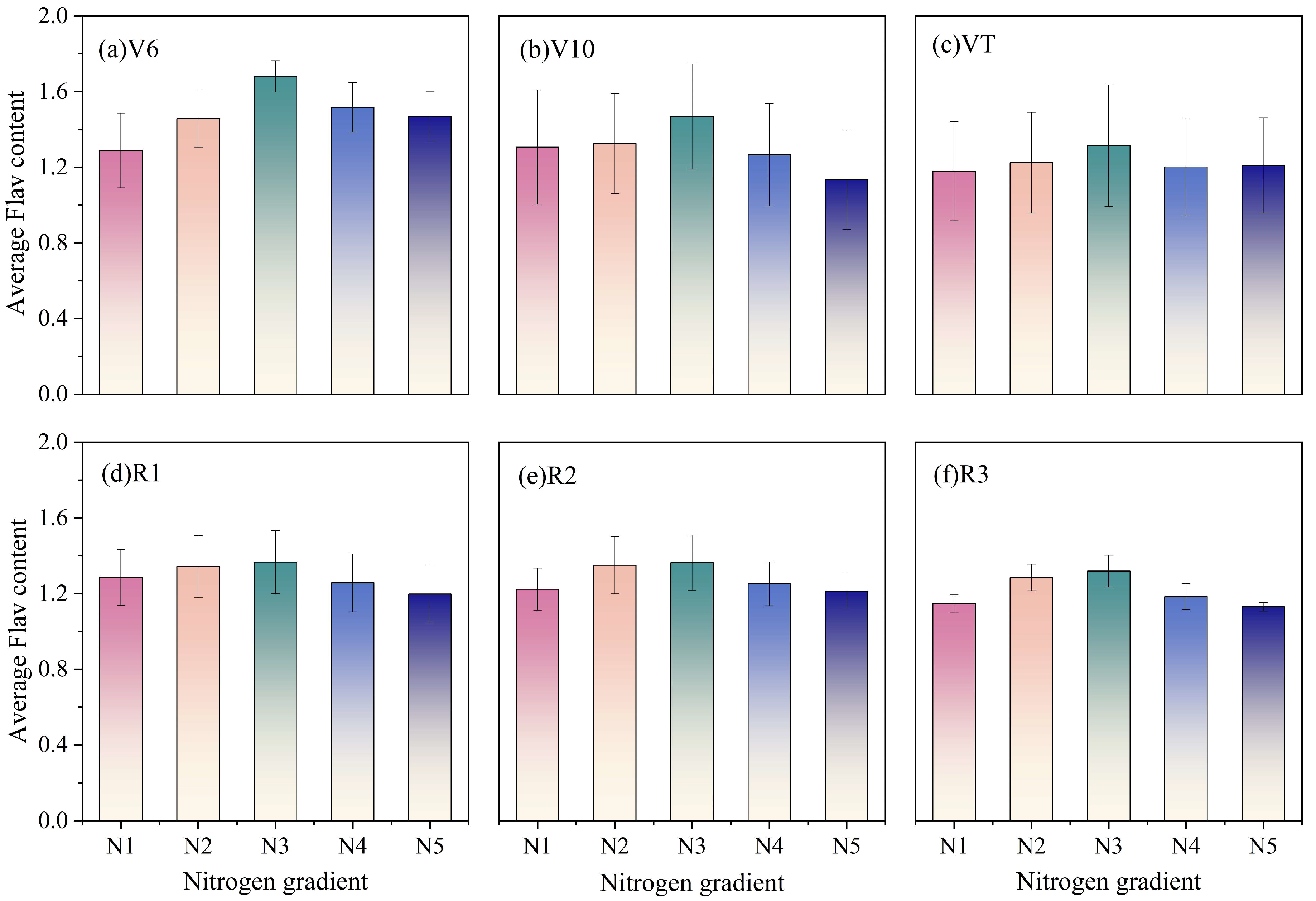
Box-and-whisker plots were used to show the distribution of Dualex-based Flav values in upper-, middle-, and lower-canopy leaves under different nitrogen rates at each growth stage (Figure 5). Overall, Flav showed clear variation among canopy positions, nitrogen levels, and growth stages. The figure shows a “hump-shaped” response of Flav to nitrogen application: concentrations rise and then fall as the nitrogen rate increases. Across stages V6 to R3, the highest Flav always occurred under the N3 treatment, with mean values of 1.6804, 1.4686, 1.3144, 1.3663, 1.3627, and 1.3184 µg cm−2 for V6, V10, VT, R1, R2, and R3, respectively. The minima appeared at N1 in V6 and VT (1.2888 and 1.1788 µg cm−2) and at N5 in V10, R1, R2, and R3 (1.1333, 1.1976, 1.2125, and 1.1299 µg cm−2). Over the whole season, the maximum Flav was recorded at V6-N3 (1.6804 µg cm−2), whereas the minimum was at R3-N5 (1.1299 µg cm−2). Large standard deviations were observed at V10 (0.2753 µg cm−2) and VT (0.2719 µg cm−2), with the highest value (0.3220 µg cm−2) occurring in VT-N3. Standard deviations at V6, R1, and R2 were similar (0.1387, 0.1568, and 0.1237 µg cm−2), while R3 showed the least variability (0.0586 µg cm−2); the smallest SD of the season occurred at R3-N5 (0.0224 µg cm−2). The hump-shaped pattern of Flav was most pronounced at V6, noticeable at V10, and largely flattened from VT onward.

3.2. Correlation Analysis of Maize Flavonoid Content

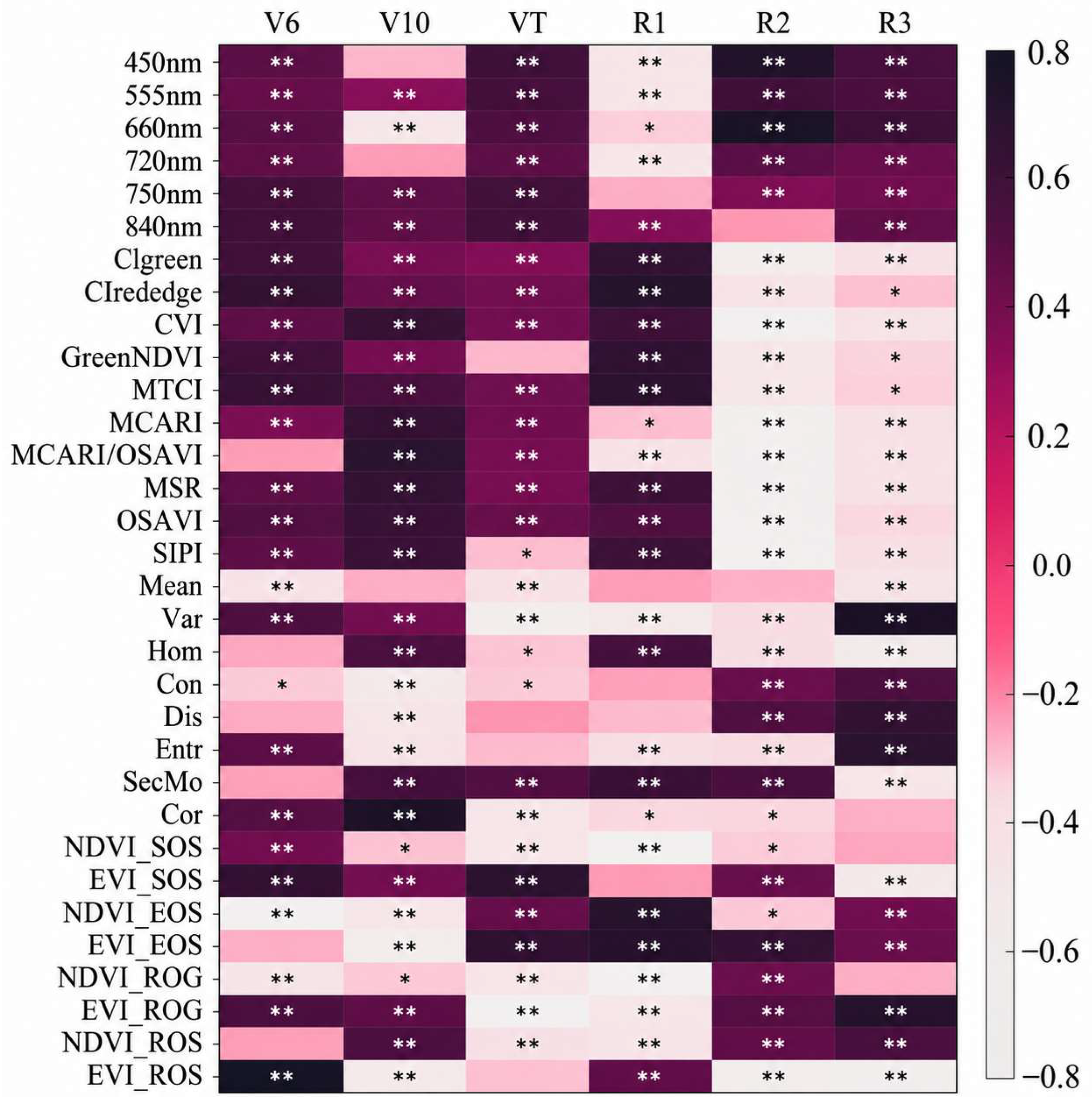
Figure 6 shows the correlations between maize leaf flavonoid (Flav) content and four groups of variables across six growth stages, including single UAV multispectral bands, conventional vegetation indices, texture features, and phenological parameters. Clear stage-dependent differences were observed. From V6 to R3, the proportions of variables significantly correlated with Flav at p < 0.01 were 78.13%, 84.38%, 78.13%, 75.00%, 84.38%, and 81.25%, respectively. The maximum absolute correlation coefficients at the six stages were 0.7902 (EVI_ROS), 0.6601 (Cor), 0.8116 (EVI_ROG), 0.6895 (CIrededge), 0.7628 (R660), and 0.7053 (Var), indicating that the dominant predictors varied with growth stage.
Among the single bands, R555 and R660 showed consistent sensitivity to Flav, and R555 remained significant at p < 0.01 throughout the season. Band-based correlations were generally stronger at V6, VT, and R3, but weaker at V10. For conventional vegetation indices, CIgreen, CIrededge, CVI, MTCI, MCARI, MSR, OSAVI, and SIPI were significant across all stages, while CIgreen, CVI, MSR, and OSAVI were consistently significant at p < 0.01. Among the texture variables, Var was the only feature that remained highly significant throughout the season, whereas Hom, Con, Entropy, SecMo, and Cor were significant in five stages. Texture features showed particularly strong responses at V10, R2, and R3. For phenological parameters, NDVI_EOS and EVI_ROG were significant across all stages, and all phenological variables reached p < 0.01 significance at V10 and R2.
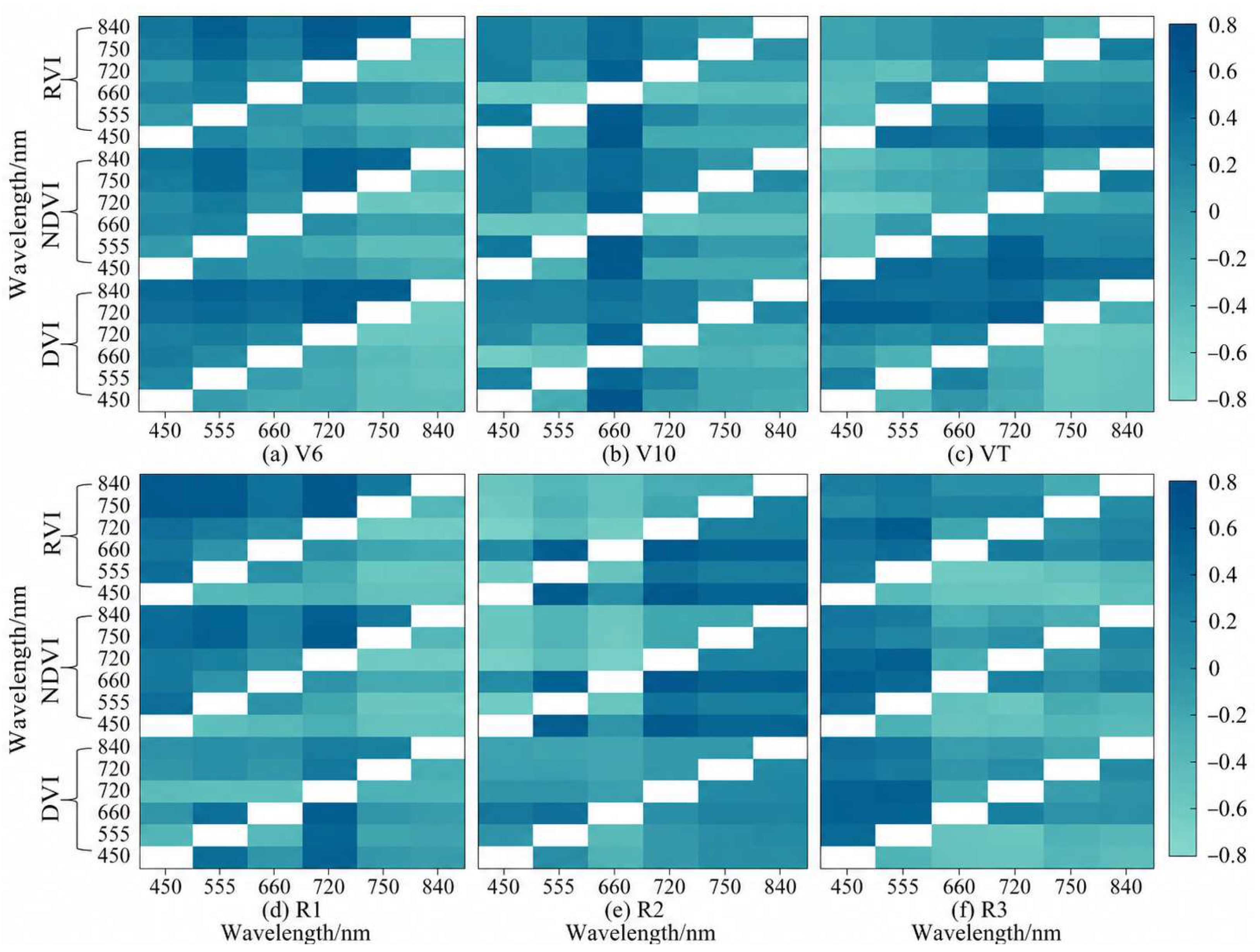
To further enhance spectral sensitivity, three optimized vegetation indices (DVI, NDVI, and RVI) were generated from all possible two-band combinations at each growth stage. Their correlation distributions are shown in Figure 7. The best-performing index type was DVI at V6 and VT, NDVI at V10, and RVI at R1, R2, and R3. The mean peak correlation coefficients from V6 to R3 were 0.3853, 0.2898, 0.3593, 0.4169, 0.4567, and 0.3367, respectively. The highest absolute correlations at each stage were 0.6293, 0.7125, 0.5912, 0.6619, 0.7989, and 0.6078, corresponding to RVI (840, 720), DVI (450, 660), RVI (450, 720), NDVI (750, 720), RVI (450, 555), and NDVI (720, 555), respectively.
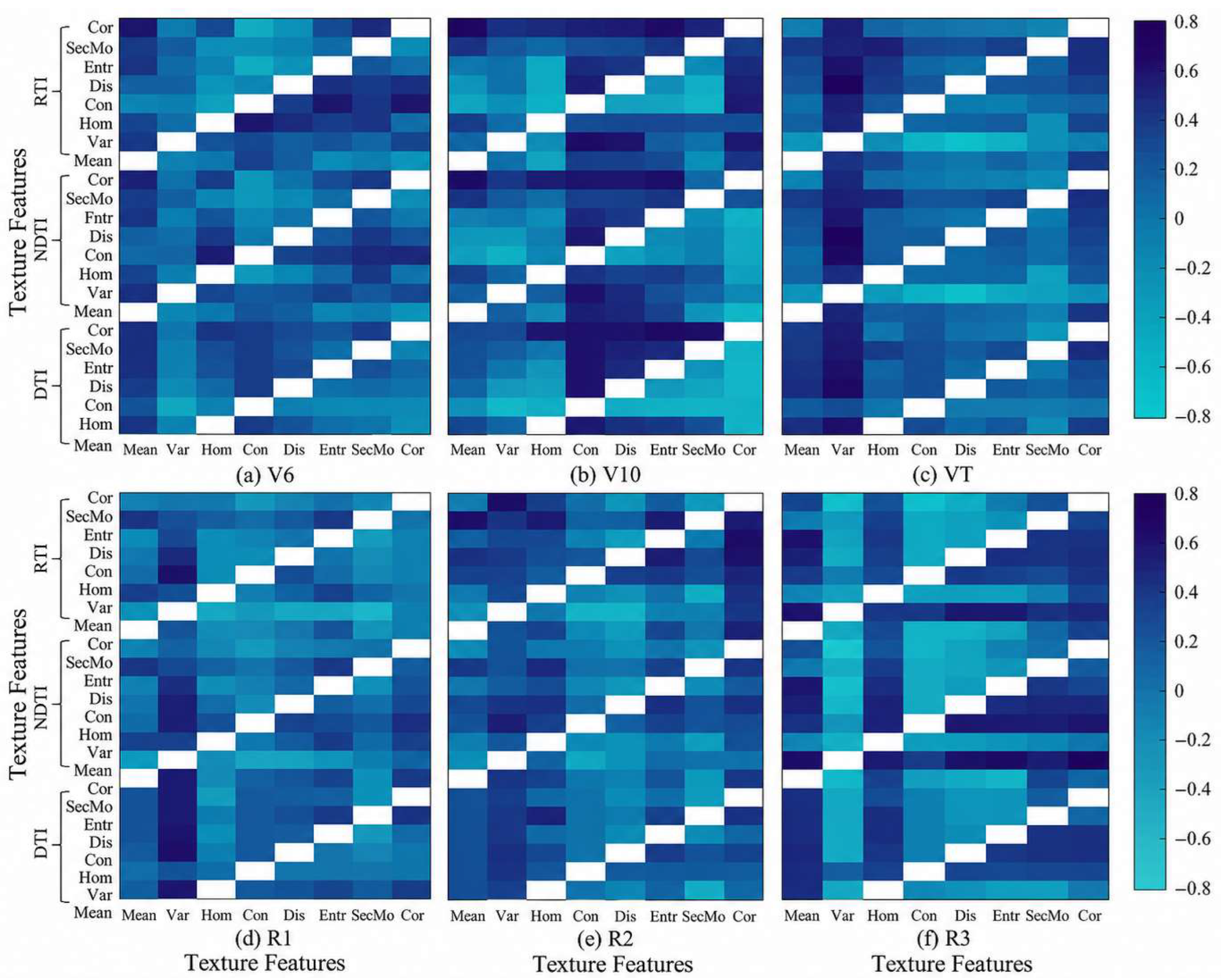
Similarly, three optimized texture indices (DTI, NDTI, and RTI) were generated from all pairwise combinations of texture features, and the corresponding correlation maps are presented in Figure 8. RTI performed best at V6, R1, and R2, DTI at V10 and VT, and NDTI at R3. The mean optimal correlation coefficients from V6 to R3 were 0.2657, 0.3416, 0.2286, 0.2533, 0.3044, and 0.4368, respectively. The highest absolute correlations at the six stages were 0.6310, 0.6368, 0.7367, 0.6583, 0.6428, and 0.7508, corresponding to RTI (Cor, Mean), RTI (Cor, Entr), NDTI (Dis, Var), DTI (Dis, Var), RTI (Entr, Cor), and RTI (Var, Mean), respectively.

3.3. Feature Selection and Model Results Analysis

Because vegetation indices and individual spectral bands showed the strongest correlations with maize Flav content, these variables were designated as the baseline predictors. Multivariate regression models were then built by adding texture descriptors and phenological parameters and applying the CARS, GA, and SPA feature selection algorithms. For each growth stage, 38 candidate variables (comprising six bands, ten VIs, three optimized VIs, eight texture metrics, three optimized texture indices, and eight phenological parameters) were submitted to CARS, GA, and SPA. The input sets differed by algorithm version: set XI included only bands plus (optimized) VIs; set XII extended XI with texture features and indices; set XIII further appended phenological parameters. This tiered strategy sought the optimal predictor combination for estimating maize Flav. A condensed summary of the feature-selection results is presented in Table 5, while the complete variable lists selected by each algorithm at each growth stage are provided in Tables S1–S3 in the Supplementary Materials.
Overall, the three feature-selection methods showed clear differences in parsimony and predictive potential. SPA retained the fewest variables and achieved the highest dimensionality reduction ratio, indicating strong compactness. By contrast, CARS generally retained more variables, suggesting a more conservative selection strategy. GA showed an intermediate tendency and, in most cases, provided a more balanced trade-off between information retention and redundancy reduction. On average, CARS, GA, and SPA retained an average of 10.11, 8.00, and 5.28 variables, corresponding to mean reduction rates of 73.39%, 78.95%, and 86.11%, respectively.
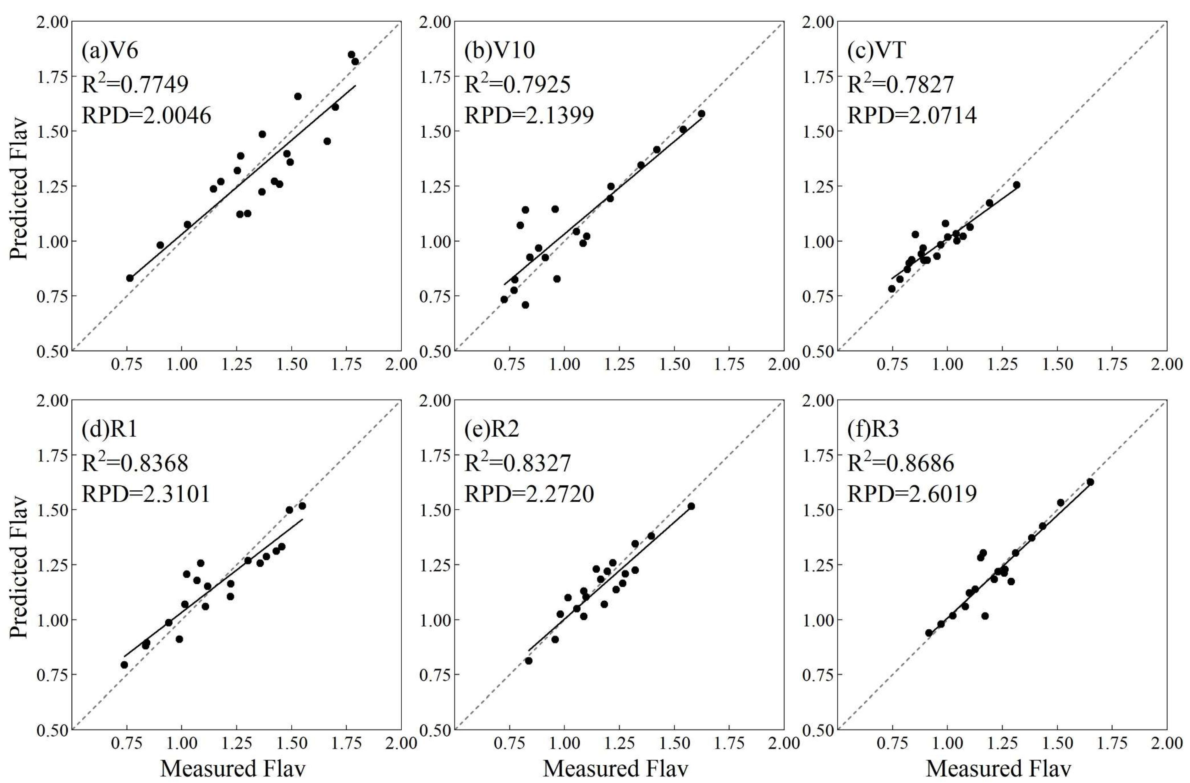
To avoid excessive figure redundancy, the detailed accuracy comparisons of all model combinations are provided in the Supplementary Materials (Figures S1–S9), while the main text focuses on the optimal model configuration and key accuracy metrics for each growth stage. Across the six growth stages (Table 6) (Figure 9), the optimal models achieved R2 values of 0.7749, 0.7925, 0.7827, 0.8368, 0.8327, and 0.8686 for V6, V10, VT, R1, R2, and R3, respectively. The corresponding RPD values were 2.0046, 2.1399, 2.0714, 2.3101, 2.2720, and 2.6019, indicating high to outstanding prediction ability. CNN provided the best performance at V6, V10, VT, and R3, whereas XGBoost was optimal at R1 and R2. These results demonstrate that the optimal estimation strategy varied across growth stages, but all stage-specific optimal models achieved reliable accuracy.

4. Discussion

4.1. Seasonal Variation in Flavonoids in Maize Leaves

Flavonoids are important indicators of maize responses to environmental stress, and their seasonal dynamics can reflect changes in plant physiological status [22,67,68]. In this study (Table 4), Flav decreased from V6 to V10, which may be associated with leaf maturation and the gradual stabilization of physiological activity. Only a slight decrease in Flav was observed from V10 to VT (Figure S10), despite continuous rainfall during this period, suggesting that short-term waterlogging induced a relatively limited Flav response under the conditions of this experiment. By contrast, Flav increased markedly from VT to R1 during a period of sustained high temperature, indicating that heat stress may have stimulated flavonoid accumulation. This pattern is consistent with the recognized protective role of flavonoids in plant stress resistance [20,21,22,23]. From R1 to R3, Flav declined again, possibly because assimilates were increasingly allocated to reproductive growth, thereby reducing the synthesis of secondary metabolites.
The response of Flav to nitrogen supply generally aligned with the Growth–Differentiation Balance Hypothesis (GDBH), which posits a trade-off between growth and secondary metabolism under varying resource conditions [69,70,71,72,73]. In this study, the five-level nitrogen treatment produced a unimodal Flav pattern (Figure 5), with moderate nitrogen favoring flavonoid accumulation. This pattern can be interpreted in terms of carbon allocation: under low nitrogen, growth and photosynthesis are limited, reducing carbon availability for secondary metabolites. Under high nitrogen, plants prioritize rapid vegetative growth and protein synthesis, which may limit carbon allocation to non-nitrogenous secondary metabolites such as flavonoids. Moderate nitrogen allows sufficient carbon assimilation without excessive growth demand, supporting flavonoid accumulation. Thus, the higher Flav values under moderate nitrogen are consistent with the growth–defense trade-off described by the GDBH. However, this interpretation provides physiological support rather than direct mechanistic confirmation, as carbon allocation, enzyme activity, and flavonoid biosynthesis were not directly measured.

4.2. Influence of Growth Stage on Flav Estimation

Model performance varied substantially among growth stages (Table 6). Overall, prediction accuracy was higher during the reproductive stages (R1, R2, and R3) than during the vegetative stages (V6, V10, and VT), which agrees with previous findings that crop phenological stage can strongly influence remote sensing retrieval performance [49].
During vegetative growth, rapid changes in leaf morphology, leaf angle, and canopy structure may weaken the consistency between canopy reflectance and leaf biochemical traits [74,75]. As a result, retrieval models are more easily affected by structural noise at V6–VT. After tasseling, canopy architecture becomes relatively stable, and the optical signal is more likely to reflect plant physiological status rather than transient structural variation. This interpretation is also supported by earlier studies showing that the relationship between maize pigment-related traits and vegetation indices tends to strengthen as development progresses [76].
From a whole-season perspective, the proposed UAV-based multisource estimation framework showed stable performance across the six maize growth stages. The optimal models at V6, V10, VT, R1, R2, and R3 all achieved RPD values above 2.0 (Figure 9), indicating reliable estimation performance during both vegetative and reproductive growth. This result suggests that the integration of multispectral, texture, and phenological descriptors can support continuous monitoring of maize Flav dynamics throughout the growing season. However, the optimal feature selection method, predictor set, and regression model differed among growth stages. Therefore, the effectiveness of the framework at the whole-season scale does not mean that a single universal model is suitable for all stages. Stage-specific modeling remains necessary because the relationships among canopy reflectance, canopy structure, phenological development, and leaf biochemical status vary during maize growth.

4.3. Effects of Feature Selection and Model Choice on Flav Estimation

The three feature selection methods differed clearly in their balance between dimensionality reduction and predictive performance (Table 5 and Tables S1–S3). SPA achieved the strongest compression, but its more aggressive variable elimination may have removed informative predictors, resulting in slightly lower and less stable model performance. CARS retained more variables, but the larger feature set did not consistently translate into higher accuracy. By comparison, GA provided a better balance between information retention and redundancy control, and therefore showed the best overall performance.
The greater contribution of texture features at certain growth stages likely reflects changes in maize canopy structure. Unlike mean spectral bands and vegetation indices, which mainly capture average canopy reflectance, GLCM-based texture features describe the spatial arrangement and local variation in image gray levels. During the late vegetative and reproductive stages, the maize canopy becomes more complex due to increased leaf overlap, canopy closure, variation in leaf angle, tassel emergence, and onset of local senescence. These structural changes increase spatial heterogeneity in UAV multispectral imagery, which can reduce the representativeness of mean spectral values alone. Texture metrics such as variance, contrast, entropy, and correlation capture canopy roughness, local contrast, and gray-level distribution, providing complementary information for Flav estimation. This explains why texture features contributed more strongly to model performance during stages with pronounced canopy structural heterogeneity. Previous studies have similarly demonstrated that texture information can enhance crop trait retrieval by mitigating the effects of illumination variation and background noise [77,78,79].
The correlation analysis and selected feature sets (Figure 6; Tables S1–S3) also highlight the relative importance of different predictor types. In general, vegetation indices and texture variables contributed more strongly than single bands, while phenological parameters further improved model performance when combined with spectral and texture information.
Among individual predictors, CIrededge and SIPI were the most informative vegetation indices, whereas NDVI_SOS and EVI_ROS contributed strongly among phenological metrics. Their importance indicates that Flav estimation is related not only to pigment-sensitive spectral responses but also to crop developmental timing and senescence dynamics. Earlier studies have also reported that SIPI is sensitive to flavonoid-related variation in crops, which supports the present findings [80].
Model comparison showed that no single algorithm was optimal across all growth stages (Figure 9). CNN performed better at several stages, likely because it captured nonlinear interactions among selected multisource features, whereas XGBoost was more effective at R1 and R2. This indicates that model suitability depends on growth stage, feature structure, and the complexity of feature interactions. Given the limited sample size at each stage and the use of selected tabular features rather than raw UAV images, model selection for stage-specific Flav estimation should balance prediction accuracy and model complexity, especially under small-sample conditions.

4.4. Spatial Mapping of Maize Flav Content

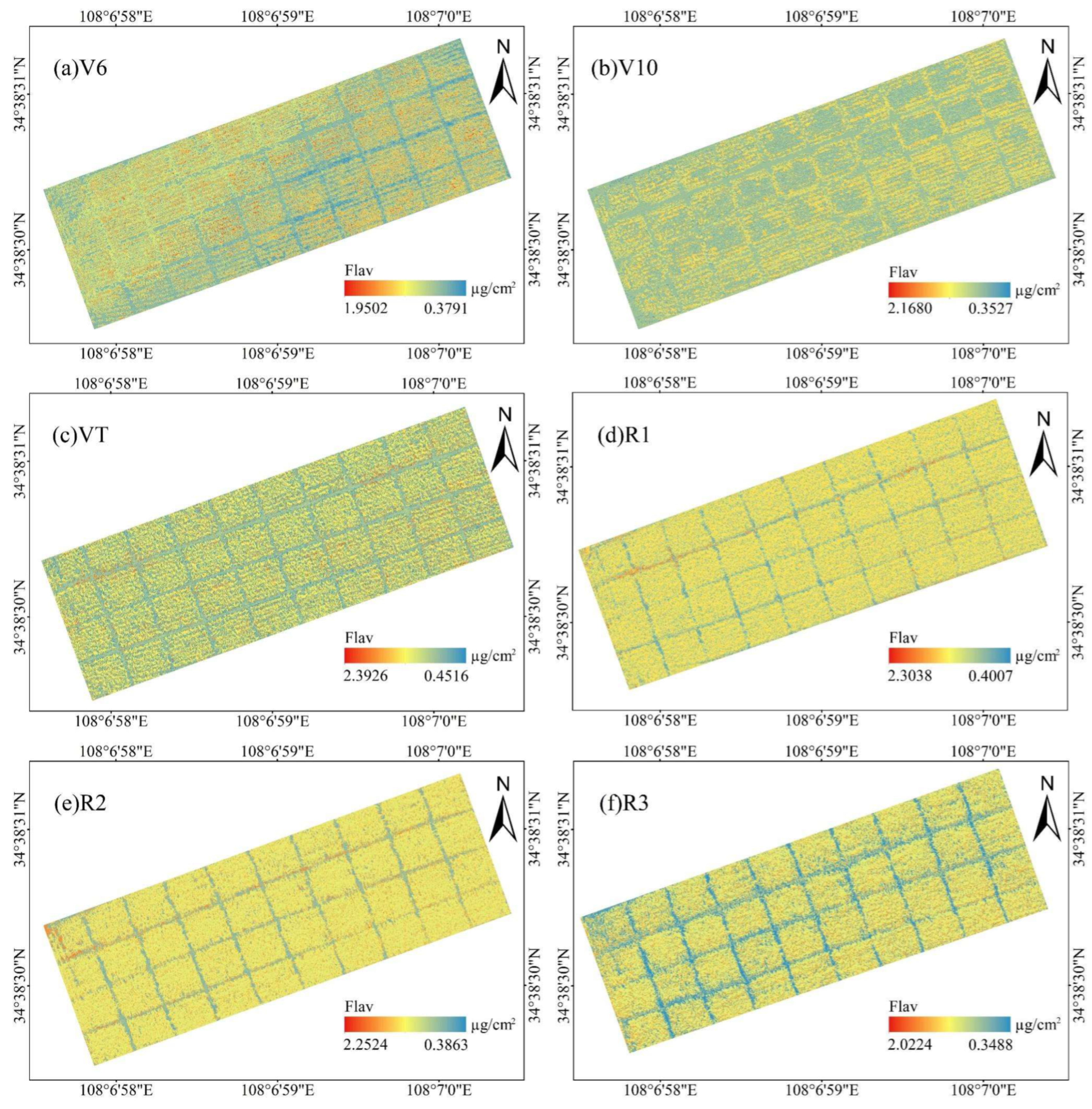
Based on the optimal feature–model combinations, spatial maps of maize canopy Flav were generated for all six growth stages (Figure 10). These maps captured clear temporal and within-field variability, indicating that UAV-based estimation can provide useful spatial information beyond point measurements. Overall, the mapped seasonal pattern was broadly consistent with field observations, showing an increase followed by a decline over the season.
Some discrepancies, however, remained between the mapped results and direct measurements. For example, the mapped peak occurred at VT rather than R1, suggesting that model uncertainty was not fully resolved. In addition, low-Flav zones observed under high-temperature (Figure S10) conditions may have been associated with temporary leaf rolling and altered canopy reflectance during midday UAV acquisition [81,82,83]. The spatial shift of high-Flav areas toward plot margins after V10 may also reflect edge effects related to light interception, nutrient distribution, or local canopy structure [84,85].

4.5. Study Limitations and Future Work

Several limitations of this study should be acknowledged. First, the dataset was collected from a single experimental site during one growing season, and the number of samples available at each growth stage was limited. Although independent test sets, five-fold cross-validation, feature selection, dropout regularization, and validation monitoring were used to reduce the risk of overfitting, the reported model performance should be interpreted as stage-specific empirical results under the present experimental conditions. External spatial and temporal validation was not conducted, and the generalization capacity of the proposed models across different years, sites, cultivars, management practices, and sensor systems remains uncertain. Future studies should therefore include multi-year, multi-site, and multi-cultivar datasets to further evaluate model transferability and robustness.
Another limitation is that the Dualex-derived Flav value used in this study represents a non-destructive optical proxy of leaf epidermal flavonoids, mainly flavonols, rather than chemically quantified total flavonoid concentration. Although the measurement principle of Dualex and previous validation studies support its application in tracking flavonoid-related variation, the quantitative relationship between Dualex readings and chemically measured flavonoid concentrations may vary with cultivar, leaf structural traits, growth stage, and environmental conditions. Future work should therefore incorporate spectrophotometric or HPLC-based measurements to establish maize-specific calibration relationships and to strengthen the physiological interpretation of UAV-based Flav estimation.
Canopy-scale Flav estimation using UAV imagery is also affected by mixed optical signals from leaf biochemical status, canopy architecture, leaf overlap, illumination conditions, soil background, and local senescence. Hybrid frameworks that combine radiative transfer models with machine learning may provide a promising way to improve the mechanistic basis of Flav estimation [86,87,88]. The inclusion of additional variables such as canopy geometry, fractional vegetation cover, air temperature, and solar radiation may further improve model robustness and generalizability under complex field conditions [89,90,91].
The phenology-related variables used in this study were derived from only six UAV acquisition dates and were therefore used as simplified temporal-context descriptors rather than fully robust phenological metrics. The duplication of the first and last observations was applied only to reduce boundary effects during logistic fitting, but it may also introduce uncertainty into the extracted descriptors. Future studies should acquire UAV time-series observations with higher temporal density to improve the robustness of phenological modeling and to better evaluate the contribution of temporal information to maize Flav estimation.
Although this study analyzed the general response of Flav to nitrogen levels, it did not fully examine the independent and interactive effects of nitrogen, phosphorus, and potassium fertilization on flavonoid metabolism. Fertilizer treatments in this study were mainly used to generate physiological variability for UAV-based model development rather than to establish a complete nutrient-response mechanism. Future research should combine remote sensing observations with factorial agronomic experiments and physiological measurements to better reveal how nutrient supply regulates maize flavonoids.

5. Conclusions

This study developed a UAV-based multisource framework for estimating Dualex-based maize Flav across six growth stages by integrating spectral, texture, and phenological features.
The integration of multisource features improved estimation accuracy compared with the use of spectral variables alone. Among the feature selection methods, GA achieved the best overall balance between dimensionality reduction and predictive performance, whereas SPA showed the strongest ability to reduce feature dimensionality. The stage-specific optimal models obtained R2 values of 0.7749–0.8686 and RPD values of 2.0046–2.6019 across the six growth stages. CNN performed best at V6, V10, VT, and R3, while XGBoost was optimal at R1 and R2. The highest accuracy was achieved at R3 using the CARS_XII–CNN model, with R2 = 0.8686, RMSEV = 0.0382, and RPD = 2.6019.
Overall, the combined use of UAV multispectral, texture, and phenological descriptors provides an effective approach for canopy-scale estimation of Dualex-based maize Flav. The results further suggest that stage-specific feature selection and modeling strategies are more suitable than a single universal model for monitoring Flav dynamics throughout the maize growth cycle.

Supplementary Materials

The following supporting information can be downloaded at: https://www.mdpi.com/article/10.3390/rs18121978/s1, Figure S1: Accuracy metrics for the multivariate PLS_XI models for estimating maize flavonoids at different growth stages. Red bars indicate the CARS method, green bars the GA method, and blue bars the SPA method; the same color coding applies to subsequent figures; Figure S2: Accuracy metrics for the multivariate PLS_XII models for estimating maize flavonoids at different growth stages; Figure S3: Accuracy metrics for the multivariate PLS_XIII models for estimating maize flavonoids at different growth stages; Figure S4: Accuracy metrics for the multivariate XGBoost_XI models for estimating maize flavonoids at different growth stages; Figure S5: Accuracy metrics for the multivariate XGBoost_XII models for estimating maize flavonoids at different growth stages; Figure S6: Accuracy metrics for the multivariate XGBoost_XIII models for estimating maize flavonoids at different growth stages; Figure S7: Accuracy metrics for the multivariate CNN_XI models for estimating maize flavonoids at different growth stages; Figure S8: Accuracy metrics for the multivariate CNN_XII models for estimating maize flavonoids at different growth stages; Figure S9: Accuracy metrics for the multivariate CNN_XIII models for estimating maize flavonoids at different growth stages; Figure S10: Daily maximum temperature and precipitation from sowing to 1 September 2024. The six maize sampling growth stages, including V6, V10, VT, R1, R2, and R3, are indicated by vertical dashed lines; Table S1: Feature variable selection from multispectral UAV data of maize leaves at different growth stages using CARS; Table S2: Feature variable selection from multispectral UAV data of maize leaves at different growth stages using GA; Table S3: Feature variable selection from multispectral UAV data of maize leaves at different growth stages using SPA.

Author Contributions

B.S.: Writing—original draft, Software, Methodology, Investigation, Data curation, Conceptualization. Y.G.: Writing—review & editing, Software, Methodology, Validation. X.F.: Software, Methodology, Validation. Z.L.: Visualization, Software. X.C.: Software, Formal analysis. Q.C.: Project administration, Funding acquisition, Supervision. All authors have read and agreed to the published version of the manuscript. We confirm that none of the material in this manuscript has been published or is under consideration for publication elsewhere.

Funding

This research was supported by the National Natural Science Foundation of China (Grant No. 41701398, Grant No. 42071240). The APC was funded by [42071240].

Data Availability Statement

The data presented in this study are available on request from the corresponding author. The data are not publicly available due to privacy or ethical restrictions.

Conflicts of Interest

The authors declare no conflicts of interest.

References

  1. Peng, Q.; Shen, R.; Li, X.; Ye, T.; Dong, J.; Fu, Y.; Yuan, W. A Twenty-Year Dataset of High-Resolution Maize Distribution in China. Sci. Data 2023, 10, 658. [Google Scholar] [CrossRef] [PubMed]
  2. Erenstein, O.; Jaleta, M.; Sonder, K.; Mottaleb, K.; Prasanna, B.M. Global Maize Production, Consumption and Trade: Trends and R&D Implications. Food Secur. 2022, 14, 1295–1319. [Google Scholar] [CrossRef]
  3. Lobell, D.B.; Schlenker, W.; Costa-Roberts, J. Climate Trends and Global Crop Production Since 1980. Science 2011, 333, 616–620. [Google Scholar] [CrossRef] [PubMed]
  4. Wheeler, T.; Von Braun, J. Climate Change Impacts on Global Food Security. Science 2013, 341, 508–513. [Google Scholar] [CrossRef] [PubMed]
  5. Rejeb, A.; Abdollahi, A.; Rejeb, K.; Treiblmaier, H. Drones in Agriculture: A Review and Bibliometric Analysis. Comput. Electron. Agric. 2022, 198, 107017. [Google Scholar] [CrossRef]
  6. Singh, A.P.; Yerudkar, A.; Mariani, V.; Iannelli, L.; Glielmo, L. A Bibliometric Review of the Use of Unmanned Aerial Vehicles in Precision Agriculture and Precision Viticulture for Sensing Applications. Remote Sens. 2022, 14, 1604. [Google Scholar] [CrossRef]
  7. Wan, L.; Zhang, J.; Dong, X.; Du, X.; Zhu, J.; Sun, D.; Liu, Y.; He, Y.; Cen, H. Unmanned Aerial Vehicle-Based Field Phenotyping of Crop Biomass Using Growth Traits Retrieved from the PROSAIL Model. Comput. Electron. Agric. 2021, 187, 106304. [Google Scholar] [CrossRef]
  8. Aasen, H.; Burkart, A.; Bolten, A.; Bareth, G. Generating 3D Hyperspectral Information with Lightweight UAV Snapshot Cameras for Vegetation Monitoring: From Camera Calibration to Quality Assurance. ISPRS J. Photogramm. Remote Sens. 2015, 108, 245–259. [Google Scholar] [CrossRef]
  9. Gao, J.; Liao, W.; Nuyttens, D.; Lootens, P.; Vangeyte, J.; Pižurica, A.; He, Y.; Pieters, J.G. Fusion of Pixel- and Object-Based Features for Weed Mapping Using Unmanned Aerial Vehicle Imagery. Int. J. Appl. Earth Obs. Geoinf. 2018, 67, 43–53. [Google Scholar] [CrossRef]
  10. Marcone, A.; Impollonia, G.; Croci, M.; Blandinières, H.; Pellegrini, N.; Amaducci, S. Garlic Yield Monitoring Using Vegetation Indices and Texture Features Derived from UAV Multispectral Imagery. Smart Agric. Technol. 2024, 8, 100513. [Google Scholar] [CrossRef]
  11. Khan, M.S.; Yadav, P.; Semwal, M.; Prasad, N.; Verma, R.K.; Kumar, D. Predicting Canopy Chlorophyll Concentration in Citronella Crop Using Machine Learning Algorithms and Spectral Vegetation Indices Derived from UAV Multispectral Imagery. Ind. Crops Prod. 2024, 219, 119147. [Google Scholar] [CrossRef]
  12. Liu, Y.; Fan, K.; Meng, L.; Nie, C.; Liu, Y.; Cheng, M.; Song, Y.; Jin, X. Synergistic Use of Stay-Green Traits and UAV Multispectral Information in Improving Maize Yield Estimation with the Random Forest Regression Algorithm. Comput. Electron. Agric. 2025, 229, 109724. [Google Scholar] [CrossRef]
  13. Ma, W.; Han, W.; Zhang, H.; Cui, X.; Zhai, X.; Zhang, L.; Shao, G.; Niu, Y.; Huang, S. UAV Multispectral Remote Sensing for the Estimation of SPAD Values at Various Growth Stages of Maize under Different Irrigation Levels. Comput. Electron. Agric. 2024, 227, 109566. [Google Scholar] [CrossRef]
  14. Pei, S.; Dai, Y.; Bai, Z.; Li, Z.; Zhang, F.; Yin, F.; Fan, J. Improved Estimation of Canopy Water Status in Cotton Using Vegetation Indices along with Textural Information from UAV-Based Multispectral Images. Comput. Electron. Agric. 2024, 224, 109176. [Google Scholar] [CrossRef]
  15. Wang, R.; Tuerxun, N.; Zheng, J. Improved Estimation of SPAD Values in Walnut Leaves by Combining Spectral, Texture, and Structural Information from UAV-Based Multispectral Images. Sci. Hortic. 2024, 328, 112940. [Google Scholar] [CrossRef]
  16. Ye, S.; Zhang, Z.; Chen, J.; Chen, H.; Zhang, B.; Bai, X.; Yang, N.; Du, R.; Yang, X.; Xu, Q.; et al. Inversion of Winter Wheat Canopy Chlorophyll Content Using Angle-Insensitive UAV-Based Spectral Indices. Comput. Electron. Agric. 2025, 230, 109902. [Google Scholar] [CrossRef]
  17. Li, Z.; Zhang, Y.; Lu, J.; Wang, Y.; Zhao, C.; Wang, W.; Wang, J.; Zhang, H.; Huo, Z. Better Inversion of Rice Nitrogen Nutrition Index at the Early Panicle Initiation Stage Using Spectral, Texture, and Wavelet Features Based on UAV Multispectral Imagery. Eur. J. Agron. 2025, 168, 127654. [Google Scholar] [CrossRef]
  18. Routaboul, J.-M.; Dubos, C.; Beck, G.; Marquis, C.; Bidzinski, P.; Loudet, O.; Lepiniec, L. Metabolite Profiling and Quantitative Genetics of Natural Variation for Flavonoids in Arabidopsis. J. Exp. Bot. 2012, 63, 3749–3764. [Google Scholar] [CrossRef] [PubMed]
  19. Wen, W.; Alseekh, S.; Fernie, A.R. Conservation and Diversification of Flavonoid Metabolism in the Plant Kingdom. Curr. Opin. Plant Biol. 2020, 55, 100–108. [Google Scholar] [CrossRef] [PubMed]
  20. Li, B.; Fan, R.; Sun, G.; Sun, T.; Fan, Y.; Bai, S.; Guo, S.; Huang, S.; Liu, J.; Zhang, H.; et al. Flavonoids Improve Drought Tolerance of Maize Seedlings by Regulating the Homeostasis of Reactive Oxygen Species. Plant Soil 2021, 461, 389–405. [Google Scholar] [CrossRef]
  21. Ferreyra, M.L.F.; Serra, P.; Casati, P. Recent Advances on the Roles of Flavonoids as Plant Protective Molecules after UV and High Light Exposure. Physiol. Plant. 2021, 173, 736–749. [Google Scholar] [CrossRef] [PubMed]
  22. Casas, M.I.; Falcone-Ferreyra, M.L.; Jiang, N.; Mejía-Guerra, M.K.; Rodríguez, E.; Wilson, T.; Engelmeier, J.; Casati, P.; Grotewold, E. Identification and Characterization of Maize Salmon Silks Genes Involved in Insecticidal Maysin Biosynthesis. Plant Cell 2016, 28, 1297–1309. [Google Scholar] [CrossRef] [PubMed]
  23. Castano-Duque, L.; Gilbert, M.K.; Mack, B.M.; Lebar, M.D.; Carter-Wientjes, C.H.; Sickler, C.M.; Cary, J.W.; Rajasekaran, K. Flavonoids Modulate the Accumulation of Toxins from Aspergillus flavus in Maize Kernels. Front. Plant Sci. 2021, 12, 761446. [Google Scholar] [CrossRef] [PubMed]
  24. Cerovic, Z.G.; Masdoumier, G.; Ghozlen, N.B.; Latouche, G. A New Optical Leaf-Clip Meter for Simultaneous Non-Destructive Assessment of Leaf Chlorophyll and Epidermal Flavonoids. Physiol. Plant. 2012, 146, 251–260. [Google Scholar] [CrossRef] [PubMed]
  25. Shi, P.; Wang, Y.; Yin, C.; Fan, K.; Qian, Y.; Chen, G. Mitigating Saturation Effects in Rice Nitrogen Estimation Using Dualex Measurements and Machine Learning. Front. Plant Sci. 2024, 15, 1518272. [Google Scholar] [CrossRef] [PubMed]
  26. Gámez, A.L.; Vatter, T.; Santesteban, L.G.; Araus, J.L.; Aranjuelo, I. On-Field Estimation of Quality Parameters in Alfalfa through Hyperspectral Spectrometer Data. Comput. Electron. Agric. 2024, 216, 108463. [Google Scholar] [CrossRef]
  27. Richardson, A.D.; Keenan, T.F.; Migliavacca, M.; Ryu, Y.; Sonnentag, O.; Toomey, M. Climate Change, Phenology, and Phenological Control of Vegetation Feedbacks to the Climate System. Agric. For. Meteorol. 2013, 169, 156–173. [Google Scholar] [CrossRef]
  28. Shen, M.; Wang, S.; Jiang, N.; Sun, J.; Cao, R.; Ling, X.; Fang, B.; Zhang, L.; Zhang, L.; Xu, X.; et al. Plant Phenology Changes and Drivers on the Qinghai–Tibetan Plateau. Nat. Rev. Earth Environ. 2022, 3, 633–651. [Google Scholar] [CrossRef]
  29. Gurung, R.B.; Breidt, F.J.; Dutin, A.; Ogle, S.M. Predicting Enhanced Vegetation Index (EVI) Curves for Ecosystem Modeling Applications. Remote Sens. Environ. 2009, 113, 2186–2193. [Google Scholar] [CrossRef]
  30. Kc, K.; Zhao, K.; Romanko, M.; Khanal, S. Assessment of the Spatial and Temporal Patterns of Cover Crops Using Remote Sensing. Remote Sens. 2021, 13, 2689. [Google Scholar] [CrossRef]
  31. Bolton, D.K.; Friedl, M.A. Forecasting Crop Yield Using Remotely Sensed Vegetation Indices and Crop Phenology Metrics. Agric. For. Meteorol. 2013, 173, 74–84. [Google Scholar] [CrossRef]
  32. Wu, L.; Zhang, Y.; Zhang, Z.; Zhang, X.; Wu, Y.; Chen, J.M. Deriving Photosystem-Level Red Chlorophyll Fluorescence Emission by Combining Leaf Chlorophyll Content and Canopy Far-Red Solar-Induced Fluorescence: Possibilities and Challenges. Remote Sens. Environ. 2024, 304, 114043. [Google Scholar] [CrossRef]
  33. Liu, X.; Peng, X.; Li, Y.; Gu, X.; Yu, L.; Wang, Y.; Cai, H. Environmental Influences on Evapotranspiration in Wheat–Maize Rotation Systems under Diverse Hydrological Regimes in the Guanzhong Plain, China. Agric. Water Manag. 2024, 306, 109204. [Google Scholar] [CrossRef]
  34. Wang, Y.; Cai, H.; Yu, L.; Peng, X.; Xu, J.; Wang, X. Evapotranspiration Partitioning and Crop Coefficient of Maize in a Dry Semi-Humid Climate Regime. Agric. Water Manag. 2020, 236, 106164. [Google Scholar] [CrossRef]
  35. Du, K.; Zhao, W.; Lv, Z.; Xu, B.; Hu, W.; Zhou, Z.; Wang, Y. Optimal Rate of Nitrogen Fertilizer Improves Maize Grain Yield by Delaying the Senescence of Ear Leaves and Thereby Altering Their Nitrogen Remobilization. Field Crops Res. 2024, 310, 109359. [Google Scholar] [CrossRef]
  36. Ji, S.; Gu, C.; Xi, X.; Zhang, Z.; Hong, Q.; Huo, Z.; Zhao, H.; Zhang, R.; Li, B.; Tan, C. Quantitative Monitoring of Leaf Area Index in Rice Based on Hyperspectral Feature Bands and Ridge Regression Algorithm. Remote Sens. 2022, 14, 2777. [Google Scholar] [CrossRef]
  37. Li, H.; Mao, Y.; Shi, H.; Fan, K.; Sun, L.; Zaman, S.; Shen, J.; Li, X.; Bi, C.; Shen, Y.; et al. Establishment of a Deep Learning Model for the Growth of Tea Cutting Seedlings Based on Hyperspectral Imaging Technique. Sci. Hortic. 2024, 331, 113106. [Google Scholar] [CrossRef]
  38. Yang, C.; Bai, J.; Sun, H.; Bi, R.; Song, L.; Muhammad, A.; Wang, C.; Zhao, Y.; Yang, W.; Xiao, L.; et al. A New Feature Selection Algorithm Combining Genetic Algorithm, Exponential Decay Function, and Machine Learning to Realize Hyperspectral Estimation of Winter Wheat Leaf Area Index. Comput. Electron. Agric. 2025, 230, 109851. [Google Scholar] [CrossRef]
  39. Chen, S.; Lou, F.; Tuo, Y.; Tan, S.; Peng, K.; Zhang, S.; Wang, Q. Prediction of Soil Water Content Based on Hyperspectral Reflectance Combined with Competitive Adaptive Reweighted Sampling and Random Frog Feature Extraction and the Back-Propagation Artificial Neural Network Method. Water 2023, 15, 2726. [Google Scholar] [CrossRef]
  40. Li, X.; Fu, X.; Li, H. A CARS–SPA–GA Feature Wavelength Selection Method Based on Hyperspectral Imaging with Potato Leaf Disease Classification. Sensors 2024, 24, 6566. [Google Scholar] [CrossRef] [PubMed]
  41. Khanal, S.; Fulton, J.; Klopfenstein, A.; Douridas, N.; Shearer, S. Integration of High-Resolution Remotely Sensed Data and Machine Learning Techniques for Spatial Prediction of Soil Properties and Corn Yield. Comput. Electron. Agric. 2018, 153, 213–225. [Google Scholar] [CrossRef]
  42. Han, H.; Lee, S.; Kim, H.-C.; Kim, M. Retrieval of Summer Sea Ice Concentration in the Pacific Arctic Ocean from AMSR2 Observations and Numerical Weather Data Using Random Forest Regression. Remote Sens. 2021, 13, 2283. [Google Scholar] [CrossRef]
  43. Araújo, M.C.U.; Saldanha, T.C.B.; Galvão, R.K.H.; Yoneyama, T.; Chame, H.C.; Visani, V. The Successive Projections Algorithm for Variable Selection in Spectroscopic Multicomponent Analysis. Chemom. Intell. Lab. Syst. 2001, 57, 65–73. [Google Scholar] [CrossRef]
  44. Akter, T.; Faqeerzada, M.A.; Kim, Y.; Pahlawan, M.F.R.; Aline, U.; Kim, H.; Kim, H.; Cho, B.-K. Hyperspectral Imaging with Multivariate Analysis for Detection of Exterior Flaws for Quality Evaluation of Apples and Pears. Postharvest Biol. Technol. 2025, 223, 113453. [Google Scholar] [CrossRef]
  45. Li, S.; Sun, L.; Jin, X.; Feng, G.; Zhang, L.; Bai, H. Research on Identification of Common Bean Seed Vigor Based on Hyperspectral and Deep Learning. Microchem. J. 2025, 211, 113133. [Google Scholar] [CrossRef]
  46. Gao, S.; Yan, K.; Liu, J.; Pu, J.; Zou, D.; Qi, J.; Mu, X.; Yan, G. Assessment of Remote-Sensed Vegetation Indices for Estimating Forest Chlorophyll Concentration. Ecol. Indic. 2024, 162, 112001. [Google Scholar] [CrossRef]
  47. Liu, S.; Bai, X.; Zhu, G.; Zhang, Y.; Li, L.; Ren, T.; Lu, J. Remote Estimation of Leaf Nitrogen Concentration in Winter Oilseed Rape across Growth Stages and Seasons by Correcting for the Canopy Structural Effect. Remote Sens. Environ. 2023, 284, 113348. [Google Scholar] [CrossRef]
  48. Wang, Y.; Yang, Z.; Kootstra, G.; Khan, H.A. The Impact of Variable Illumination on Vegetation Indices and Evaluation of Illumination Correction Methods on Chlorophyll Content Estimation Using UAV Imagery. Plant Methods 2023, 19, 51. [Google Scholar] [CrossRef] [PubMed]
  49. Schlemmer, M.; Gitelson, A.; Schepers, J.; Ferguson, R.; Peng, Y.; Shanahan, J.; Rundquist, D. Remote Estimation of Nitrogen and Chlorophyll Contents in Maize at Leaf and Canopy Levels. Int. J. Appl. Earth Obs. Geoinf. 2013, 25, 47–54. [Google Scholar] [CrossRef]
  50. Vincini, M.; Frazzi, E. Comparing Narrow- and Broad-Band Vegetation Indices to Estimate Leaf Chlorophyll Content in Planophile Crop Canopies. Precis. Agric. 2011, 12, 334–344. [Google Scholar] [CrossRef]
  51. Daughtry, C.; Walthall, C.L.; Kim, M.S.; De Colstoun, E.B.; McMurtrey, J.E., III. Estimating Corn Leaf Chlorophyll Concentration from Leaf and Canopy Reflectance. Remote Sens. Environ. 2000, 74, 229–239. [Google Scholar] [CrossRef]
  52. Wu, C.; Niu, Z.; Tang, Q.; Huang, W. Estimating Chlorophyll Content from Hyperspectral Vegetation Indices: Modeling and Validation. Agric. For. Meteorol. 2008, 148, 1230–1241. [Google Scholar] [CrossRef]
  53. Rondeaux, G.; Steven, M.; Baret, F. Optimization of Soil-Adjusted Vegetation Indices. Remote Sens. Environ. 1996, 55, 95–107. [Google Scholar] [CrossRef]
  54. Jay, S.; Gorretta, N.; Morel, J.; Maupas, F.; Bendoula, R.; Rabatel, G.; Dutartre, D.; Comar, A.; Baret, F. Estimating Leaf Chlorophyll Content in Sugar Beet Canopies Using Millimeter- to Centimeter-Scale Reflectance Imagery. Remote Sens. Environ. 2017, 198, 173–186. [Google Scholar] [CrossRef]
  55. Wang, Y.; Shi, H.; Yang, X.; Jiang, Y.; Wu, Y.; Shui, J.; Liu, Y.; Guo, M.; Li, L. Spatial Downscaling of SMAP Soil Moisture to High Resolution Using Machine Learning over China’s Loess Plateau. Catena 2024, 247, 108492. [Google Scholar] [CrossRef]
  56. Hu, X.; Shi, L.; Lin, L.; Li, S.; Deng, X.; Li, J.; Bian, J.; Su, C.; Du, S.; Wang, T.; et al. Accurate Estimation of Gross Primary Production of Paddy Rice Cropland with UAV Imagery-Driven Leaf Biochemical Model. Remote Sens. 2024, 16, 3906. [Google Scholar] [CrossRef]
  57. Hlatshwayo, S.T.; Mutanga, O.; Lottering, R.T.; Kiala, Z.; Ismail, R. Mapping Forest Aboveground Biomass in the Reforested Buffelsdraai Landfill Site Using Texture Combinations Computed from SPOT-6 Pan-Sharpened Imagery. Int. J. Appl. Earth Obs. Geoinf. 2019, 74, 65–77. [Google Scholar] [CrossRef]
  58. Zhang, J.; Xiao, J.; Tong, X.; Zhang, J.; Meng, P.; Li, J.; Liu, P.; Yu, P. NIRv and SIF Better Estimate Phenology than NDVI and EVI: Effects of Spring and Autumn Phenology on Ecosystem Production of Planted Forests. Agric. For. Meteorol. 2022, 315, 108819. [Google Scholar] [CrossRef]
  59. Xue, Z.; Du, P.; Feng, L. Phenology-Driven Land Cover Classification and Trend Analysis Based on Long-Term Remote Sensing Image Series. IEEE J. Sel. Top. Appl. Earth Obs. Remote Sens. 2014, 7, 1142–1156. [Google Scholar] [CrossRef]
  60. Zhuang, J.; Wang, Q. Estimating Leaf Chlorophyll Fluorescence Parameters Using Partial Least Squares Regression with Fractional-Order Derivative Spectra and Effective Feature Selection. Remote Sens. 2025, 17, 833. [Google Scholar] [CrossRef]
  61. Chen, Z.; Pan, X.; Wu, T.; Shi, T.; Lei, J.; Li, Y.; Chen, X.; Huang, J.; Wang, Z.; Chen, Y. Improved Mangrove α-Diversity Estimation by Coupling Multispectral Satellite Images, Canopy Traits and Soil Properties. Catena 2025, 251, 108813. [Google Scholar] [CrossRef]
  62. Lin, N.; Zhang, D.; Feng, S.; Ding, K.; Tan, L.; Wang, B.; Chen, T.; Li, W.; Dai, X.; Pan, J.; et al. Rapid Landslide Extraction from High-Resolution Remote Sensing Images Using SHAP-OPT-XGBoost. Remote Sens. 2023, 15, 3901. [Google Scholar] [CrossRef]
  63. He, J.; Shi, Y.; Xu, L.; Lu, Z.; Feng, M.; Tang, J.; Guo, X. Exploring the Scale Effect of Urban Thermal Environment through an XGBoost Model. Sustain. Cities Soc. 2024, 114, 105763. [Google Scholar] [CrossRef]
  64. Zhang, J.; Zhang, D.; Cai, Z.; Wang, L.; Wang, J.; Sun, L.; Fan, X.; Shen, S.; Zhao, J. Spectral Technology and Multispectral Imaging for Estimating the Photosynthetic Pigments and SPAD of Chinese Cabbage Based on Machine Learning. Comput. Electron. Agric. 2022, 195, 106814. [Google Scholar] [CrossRef]
  65. Ye, Z.; Tan, X.; Dai, M.; Chen, X.; Zhong, Y.; Zhang, Y.; Ruan, Y.; Kong, D. A Hyperspectral Deep Learning Attention Model for Predicting Lettuce Chlorophyll Content. Plant Methods 2024, 20, 22. [Google Scholar] [CrossRef] [PubMed]
  66. Viscarra Rossel, R.A.; McGlynn, R.N.; McBratney, A.B. Determining the Composition of Mineral–Organic Mixes Using UV–Vis–NIR Diffuse Reflectance Spectroscopy. Geoderma 2006, 137, 70–82. [Google Scholar] [CrossRef]
  67. Dong, Q.; Zhao, X.; Zhou, D.; Liu, Z.; Shi, X.; Yuan, Y.; Jia, P.; Liu, Y.; Song, P.; Wang, X.; et al. Maize and Peanut Intercropping Improves the Nitrogen Accumulation and Yield per Plant of Maize by Promoting the Secretion of Flavonoids and Abundance of Bradyrhizobium in the Rhizosphere. Front. Plant Sci. 2022, 13, 957336. [Google Scholar] [CrossRef] [PubMed]
  68. Han, Z.; Zheng, Y.; Zhang, X.; Wang, B.; Guo, Y.; Guan, Z. Flavonoid Metabolism Plays an Important Role in Response to Lead Stress in Maize at the Seedling Stage. BMC Plant Biol. 2024, 24, 726. [Google Scholar] [CrossRef] [PubMed]
  69. Loomis, W. Growth-Differentiation Balance vs. Carbohydrate–Nitrogen Ratio. Proc. Am. Soc. Hortic. Sci. 1932, 29, 240–245. [Google Scholar]
  70. Herms, D.A.; Mattson, W.J. The Dilemma of Plants: To Grow or Defend. Q. Rev. Biol. 1992, 67, 283–335. [Google Scholar] [CrossRef]
  71. Van Velzen, E.; Etienne, R.S. The Importance of Ecological Costs for the Evolution of Plant Defense against Herbivory. J. Theor. Biol. 2015, 372, 89–99. [Google Scholar] [CrossRef] [PubMed]
  72. Walter, S.; Zehring, J.; Mink, K.; Ramminger, S.; Quendt, U.; Zocher, K.; Rohn, S. Analysis and Correlations of the Protein Content and Selected ‘Antinutrients’ of Faba Beans (Vicia faba) in a German Sample Set of the Cultivation Years 2016, 2017, and 2018. J. Sci. Food Agric. 2023, 103, 729–737. [Google Scholar] [CrossRef]
  73. Stamp, N. Out of the Quagmire of Plant Defense Hypotheses. Q. Rev. Biol. 2003, 78, 23–55. [Google Scholar] [CrossRef]
  74. Kosola, K.R.; Eller, M.S.; Dohleman, F.G.; Olmedo-Pico, L.; Bernhard, B.; Winans, E.; Barten, T.J.; Brzostowski, L.; Murphy, L.R.; Gu, C.; et al. Short-Stature and Tall Maize Hybrids Have a Similar Yield Response to Split-Rate vs. Pre-Plant N Applications, but Differ in Biomass and Nitrogen Partitioning. Field Crops Res. 2023, 295, 108880. [Google Scholar] [CrossRef]
  75. Széles, A.; Horváth, É.; Simon, K.; Zagyi, P.; Huzsvai, L. Maize Production under Drought Stress: Nutrient Supply, Yield Prediction. Plants 2023, 12, 3301. [Google Scholar] [CrossRef] [PubMed]
  76. Guo, Y.; Wang, H.; Wu, Z.; Wang, S.; Sun, H.; Senthilnath, J.; Wang, J.; Bryant, R.C.; Fu, Y. Modified Red–Blue Vegetation Index for Chlorophyll Estimation and Yield Prediction of Maize from Visible Images Captured by UAV. Sensors 2020, 20, 5055. [Google Scholar] [CrossRef] [PubMed]
  77. Yuan, W.; Meng, Y.; Li, Y.; Ji, Z.; Kong, Q.; Gao, R.; Su, Z. Research on Rice Leaf Area Index Estimation Based on Fusion of Texture and Spectral Information. Comput. Electron. Agric. 2023, 211, 108016. [Google Scholar] [CrossRef]
  78. Zhang, X.; Zhang, K.; Sun, Y.; Zhao, Y.; Zhuang, H.; Ban, W.; Chen, Y.; Fu, E.; Chen, S.; Liu, J.; et al. Combining Spectral and Texture Features of UAS-Based Multispectral Images for Maize Leaf Area Index Estimation. Remote Sens. 2022, 14, 331. [Google Scholar] [CrossRef]
  79. Zou, M.; Liu, Y.; Fu, M.; Li, C.; Zhou, Z.; Meng, H.; Xing, E.; Ren, Y. Combining Spectral and Texture Features of UAV Images with Plant Height to Improve LAI Estimation of Winter Wheat at the Jointing Stage. Front. Plant Sci. 2024, 14, 1272049. [Google Scholar] [CrossRef] [PubMed]
  80. Falcioni, R.; Antunes, W.C.; Demattê, J.A.M.; Nanni, M.R. Reflectance Spectroscopy for the Classification and Prediction of Pigments in Agronomic Crops. Plants 2023, 12, 2347. [Google Scholar] [CrossRef]
  81. Hu, J.; Zhao, X.; Gu, L.; Liu, P.; Zhao, B.; Zhang, J.; Ren, B. The Effects of High Temperature, Drought, and Their Combined Stresses on the Photosynthesis and Senescence of Summer Maize. Agric. Water Manag. 2023, 289, 108525. [Google Scholar] [CrossRef]
  82. Kadioglu, A.; Terzi, R.; Saruhan, N.; Saglam, A. Current Advances in the Investigation of Leaf Rolling Caused by Biotic and Abiotic Stress Factors. Plant Sci. 2012, 182, 42–48. [Google Scholar] [CrossRef]
  83. Wang, Y.; Jing, X.; Gao, Y.; Han, X.; Zhao, C.; Pan, W. Leaf Rolling Detection in Maize under Complex Environments Using an Improved Deep Learning Method. Plant Mol. Biol. 2024, 114, 92. [Google Scholar] [CrossRef] [PubMed]
  84. Shen, L.; Wang, X.; Liu, T.; Wei, W.; Zhang, S.; Keyhani, A.B.; Li, L.; Zhang, W. Border Row Effects on the Distribution of Root and Soil Resources in Maize–Soybean Strip Intercropping Systems. Soil Tillage Res. 2023, 233, 105812. [Google Scholar] [CrossRef]
  85. Wang, R.; Sun, Z.; Bai, W.; Wang, E.; Wang, Q.; Zhang, D.; Zhang, Y.; Yang, N.; Liu, Y.; Nie, J.; et al. Canopy Heterogeneity with Border-Row Proportion Affects Light Interception and Use Efficiency in Maize/Peanut Strip Intercropping. Field Crops Res. 2021, 271, 108239. [Google Scholar] [CrossRef]
  86. Kim, Y.J.; Kim, W.; Im, J.; Choi, J.; Lee, S. Atmospheric-Correction-Free Red Tide Quantification Algorithm for GOCI Based on Machine Learning Combined with a Radiative Transfer Simulation. ISPRS J. Photogramm. Remote Sens. 2023, 199, 197–213. [Google Scholar] [CrossRef]
  87. Xie, Q.; Dash, J.; Huete, A.; Jiang, A.; Yin, G.; Ding, Y.; Peng, D.; Hall, C.C.; Brown, L.; Shi, Y.; et al. Retrieval of Crop Biophysical Parameters from Sentinel-2 Remote Sensing Imagery. Int. J. Appl. Earth Obs. Geoinf. 2019, 80, 187–195. [Google Scholar] [CrossRef]
  88. Zérah, Y.; Valero, S.; Inglada, J. Physics-Constrained Deep Learning for Biophysical Parameter Retrieval from Sentinel-2 Images: Inversion of the PROSAIL Model. Remote Sens. Environ. 2024, 312, 114309. [Google Scholar] [CrossRef]
  89. Liao, D.; Niu, J.; Lu, N.; Shen, Q. Towards Crop Yield Estimation at a Finer Spatial Resolution Using Machine Learning Methods over Agricultural Regions. Theor. Appl. Climatol. 2021, 146, 1387–1401. [Google Scholar] [CrossRef]
  90. Liu, J.; You, Y.; Li, J.; Sitch, S.; Gu, X.; Nabel, J.E.M.S.; Lombardozzi, D.; Luo, M.; Feng, X.; Arneth, A.; et al. Response of Global Land Evapotranspiration to Climate Change, Elevated CO2, and Land Use Change. Agric. For. Meteorol. 2021, 311, 108663. [Google Scholar] [CrossRef]
  91. Zhan, W.; Yang, X.; Ryu, Y.; Dechant, B.; Huang, Y.; Goulas, Y.; Kang, M.; Gentine, P. Two for One: Partitioning CO2 Fluxes and Understanding the Relationship between Solar-Induced Chlorophyll Fluorescence and Gross Primary Productivity Using Machine Learning. Agric. For. Meteorol. 2022, 321, 108980. [Google Scholar] [CrossRef]
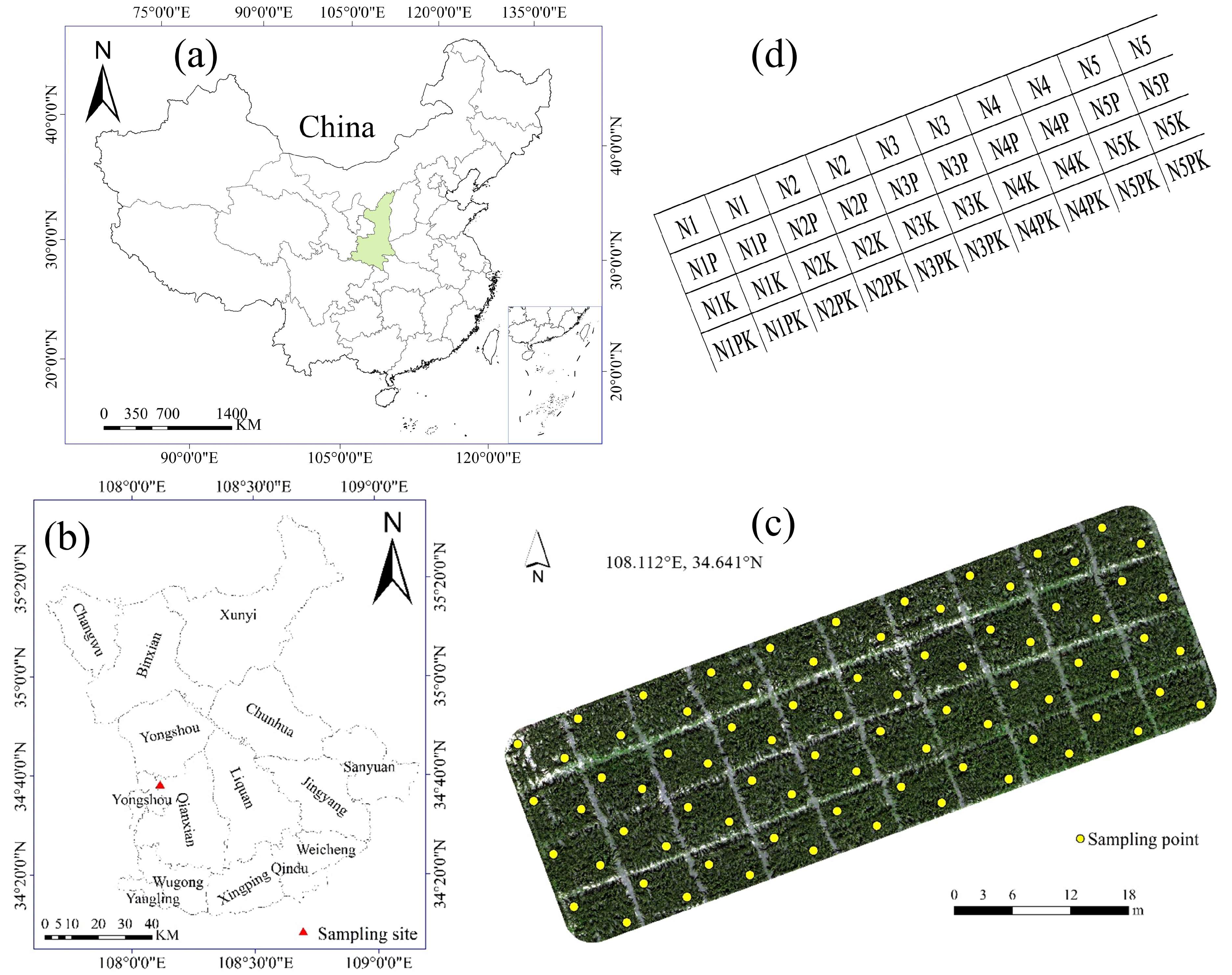
Figure 1. Location and experimental layout of the study area: (a) location of Shaanxi Province in China; (b) location of Qian County in Shaanxi Province; (c) UAV-based orthomosaic of the experimental field, with yellow circles indicating sampling points; (d) fertilization treatment layout of the 40 plots. The red triangle marks the study area.
Remotesensing 18 01978 g001
Figure 2. Sampling of flavonoid content in maize leaves: panels (af) show field scenes at the V6, V10, VT, R1, R2, and R3 growth stages, respectively; (g) denotes the measurement positions; (h) colored tags identify the sampled plants and leaves; (i) Dualex Scientific + multifunctional leaf meter.
Remotesensing 18 01978 g002
Figure 3. UAV multispectral data acquisition: (a) M300 RTK unmanned aerial vehicle; (b) MS600 Pro multispectral camera covering the 450, 555, 660, 720, 750, and 840 nm bands; (c) UAV in-flight operation; (d) true-color composite of the captured imagery.
Remotesensing 18 01978 g003
Figure 4. Technical workflow for retrieving Dualex-based maize Flav values using UAV multispectral imagery. The workflow includes field Dualex measurements, UAV image acquisition, multisource feature construction, predictor-set design, feature selection, model construction, accuracy assessment, stage-specific optimal model identification, and spatial mapping. XI represents spectral bands plus conventional and optimized vegetation indices; XII represents XI plus texture features and texture indices; XIII represents XII plus phenological parameters.
Remotesensing 18 01978 g004
Figure 5. Box-and-whisker plots showing the distribution of Dualex-based Flav values in upper-, middle-, and lower-canopy maize leaves under different nitrogen rates at each growth stage. N1, N2, N3, N4, and N5 correspond to nitrogen applications of 50, 100, 150, 200, and 250 kg ha−1, respectively.
Remotesensing 18 01978 g005
Figure 6. Pearson correlation coefficients between Dualex-based maize Flav and single bands, vegetation indices, texture features, and phenological parameters at each growth stage. Positive and negative values indicate the direction of association, and color intensity indicates correlation strength. Significance was assessed using a two-tailed t-test. * and ** indicate significance at p < 0.05 and p < 0.01, respectively.
Remotesensing 18 01978 g006
Figure 7. Pearson correlation heatmap between optimized vegetation indices and Dualex-based maize Flav at each growth stage.
Remotesensing 18 01978 g007
Figure 8. Pearson correlation heatmap between optimized texture indices and Dualex-based maize Flav at each growth stage.
Remotesensing 18 01978 g008
Figure 9. Validation results for the optimal Flav estimation models at each growth stage. The dashed line represents the 1:1 reference, while the solid line indicates the fitted regression curve.
Remotesensing 18 01978 g009
Figure 10. Spatial distribution of estimated Flav content in the maize canopy across the study area.
Remotesensing 18 01978 g010
Table 1. Vegetation indices used in this study.
Spectral IndicesEquationsReferences
CIgreen R N I R / R g r e e n 1 [49]
CIrededge ( R N I R / R r e d e d g e ) 1 [49]
CVI ( R N I R / R g r e e n ) ( R r e d / R g r e e n ) [50]
GreenNDVI ( R N I R R g r e e n ) / ( R N I R + R g r e e n ) [50]
MTCI ( R N I R R r e d e d g e ) / ( R r e d e d g e + R r e d ) [49]
MCARI ρ 700 ρ 670 0.2 ρ 700 ρ 550 ρ 700 / ρ 670 [51]
MCARI/OSAVI ρ 700 ρ 670 0.2 ρ 700 ρ 550 ρ 700 / ρ 670 / 1 + 0.16 ρ 800 ρ 670 / ρ 800 + ρ 670 + 0.16 [51]
MSR ρ 800 / ρ 670 1 / ρ 800 / ρ 670 + 1 [52]
OSAVI 1 + 0.16 ρ 800 ρ 670 / ρ 800 + ρ 670 + 0.16 [53]
SIPI ρ 850 ρ 445 / ρ 850 + ρ 680 [54]
Note: Band ranges—green: 540–560 nm; red: 660–680 nm; red-edge: 690–750 nm; NIR: 780–800 nm. ρ denotes the reflectance within the specified band.
Table 2. Optimized spectral indices used in this study.
Spectral IndicesEquations
RVI ρ x / ρ y
DVI ρ x ρ y
NDVI ρ x ρ y / ρ x + ρ y
Note: ρx and ρy represent reflectance at x and y nm, respectively.
Table 3. Texture indices and their computation formulae.
Texture IndexEquations
DTI T 1 T 2
NDTI T 1 T 2 / T 1 + T 2
RTI T 1 / T 2
Note: T1 and T2 denote any two selected GLCM texture metrics from the eight extracted texture variables, namely mean, variance, homogeneity, contrast, dissimilarity, entropy, second moment, and correlation.
Table 4. Statistics of measured flavonoid content in maize leaves across growth stages and canopy positions.
Growth
Stages
Sample
Numbers
LayerRangeMeanStandard
Deviation
Coefficient of
Variation (%)
V6237Upper0.6620–1.86761.36741.48240.2820.76
Middle0.6764–1.86221.44880.2920.20
Basal 0.9142–1.93881.63110.1811.00
V10240Upper0.6706–1.62351.03451.30610.2624.99
Middle0.6291–1.79761.30430.2821.20
Basal 0.7835–1.97291.57940.3018.89
VT240Upper0.5836–1.37770.95411.21370.1515.74
Middle0.5458–1.68501.19550.2621.39
Basal 0.5572–1.98841.49160.3221.64
R1240Upper0.7395–1.58401.16271.30330.2319.81
Middle0.6279–1.69481.27230.2620.07
Basal 0.7211–1.92291.47500.2818.77
R2240Upper0.7965–1.61971.16841.29880.1714.19
Middle0.8180–1.82001.29880.2418.16
Basal 0.5896–1.89641.42920.3322.78
R3237Upper0.6197–1.79131.20551.23190.2117.24
Middle0.6705–1.80741.18910.2319.38
Basal 0.7335–1.88901.30120.3023.04
Table 5. Numbers of selected variables and reduction ratios obtained by CARS, GA, and SPA for different predictor sets at six maize growth stages.
Growth StageMethodPredictor SetSelected VariablesReduction Ratio (%)
V6CARSXIII1171.05
GAXIII878.95
SPAXIII684.21
V10CARSXII1365.79
GAXIII878.95
SPAXIII586.84
VTCARSXII1268.42
GAXIII878.95
SPAXII489.47
R1CARSXIII878.95
GAXIII878.95
SPAXIII878.95
R2CARSXII1171.05
GAXII878.95
SPAXIII586.84
R3CARSXII1268.42
GAXIII878.95
SPAXIII684.21
Note: Table 5 presents a concise summary of the feature selection results, while the complete lists of variables selected by each algorithm at each growth stage are provided in Supplementary Tables S1–S3. The input predictor sets differed by version: set XI included only spectral bands and conventional/optimized vegetation indices; set XII extended set XI by adding texture features and texture indices; set XIII further incorporated phenological parameters.
Table 6. Best performing model configuration for maize Flav estimation at each growth stage.
Growth StageBest ConfigurationPredictor SetSelectorModelR2RMSEVRPD
V6CARS_XIII–CNNXIIICARSCNN0.77490.09322.0046
V10CARS_XII–CNNXIICARSCNN0.79250.07732.1399
VTSPA_XII–CNNXIISPACNN0.78270.04602.0714
R1SPA_XIII–XGBoostXIIISPAXGBoost0.83680.06732.3101
R2GA_XII–XGBoostXIIGAXGBoost0.83270.04592.2720
R3CARS_XII–CNNXIICARSCNN0.86860.03822.6019
Disclaimer/Publisher’s Note: The statements, opinions and data contained in all publications are solely those of the individual author(s) and contributor(s) and not of MDPI and/or the editor(s). MDPI and/or the editor(s) disclaim responsibility for any injury to people or property resulting from any ideas, methods, instructions or products referred to in the content.