Compensation of the Propagation and Clutter Effects of Rainfall for Pol-SAR-Based Sea-Surface Target Detection

Highlights

What are the main findings?

• Rain-induced signal loss and rain clutter act together rather than independently to reduce ship visibility in polarimetric SAR images.
• Compensating for rainfall effects before optimizing the receive polarization can recover ship visibility without prior knowledge of the target scattering pattern.

What are the implications of the main findings?

• The proposed method improves target enhancement by 4–13 dB over conventional polarimetric filtering and performs close to an ideal matched filter.
• This framework indicates a potential route for reducing rain-induced degradation in Pol-SAR maritime target detection, where attenuation and clutter jointly degrade imagery.

Abstract

Polarimetric synthetic aperture radar (Pol-SAR) is one of the most important approaches for sea-surface target detection, but under rainfall conditions it tends to be distorted by the electromagnetic (EM) propagation effects and clutter interference of rainfall. To address this problem, this paper proposes a joint compensation method to mitigate the impacts of rainfall on the detection of sea-surface targets. In the method, a composite imaging model that thoroughly takes into account the propagation and scattering effects of rainfall, sea surface, and ship targets is first established. Then, a range-wise algorithm is proposed to effectively estimate the propagation effects, which are used to compensate for the radar echoes distorted by rainfall. Consequently, a hierarchical search strategy is employed to optimize the receiving polarization state to better discriminate the targets from rainfall and sea clutter. Simulation results show that, across the tested sea-surface wind and rainfall conditions, the proposed method improves the signal-to-clutter-plus-noise ratio (SCNR) by 4 to 13 dB compared with the polarimetric whitening filter, demonstrating its effectiveness under coupled rain–sea conditions.

1. Introduction

Synthetic aperture radar (SAR) can provide high-resolution images under all-day and all-weather conditions, and has become an important tool for Earth observation, maritime surveillance, and target recognition [1]. In addition to time, frequency, and spatial information, polarization provides another dimension for describing target scattering in complex environments [2]. For maritime applications, polarimetric SAR (Pol-SAR) offers full-polarimetric scattering information, which helps distinguish ships from strong sea clutter and improves the reliability of target discrimination [3,4].

Even with polarimetric information, ship detection in Pol-SAR images remains difficult when sea clutter is strong, target echoes are weak, or vessels are densely distributed [5]. Prior work has developed mainly along two directions. One exploits motion contrast between ships and the sea. This line has progressed from single-channel processing to multichannel schemes and includes joint space-time polarization detection [6,7], interferometric optimization [8], multi-sub-aperture differencing [9], and along-track interferometry combined with constant false alarm rate (CFAR) for improved velocity estimation [10]. The other direction focuses on polarimetric scattering behavior. Early detectors relied largely on channel synthesis [11], whereas later studies introduced statistical formulations such as the polarimetric matched filter [12] and the prior-free polarimetric whitening filter [13]. Physical scattering characteristics were then incorporated to further increase target-to-clutter contrast, including sea-surface reflection symmetry [14], polarimetric notch filtering [15,16], subspace projection, and multi-model decomposition of ship superstructure scattering [17,18,19]. Deep-learning methods have also been explored because of their multiscale feature representation. Recent marine object detection studies have further improved image-domain representation through prototype self-distillation [20], density-aware vessel representation [21], sparsity-aware feature modeling [22], and distributed or collaborative learning [23]. These learning-based detectors are complementary to the present physics-guided framework, which focuses on rain-induced propagation distortion and additive hydrometeor clutter before detection. Even so, most existing studies are still developed under clear or spatially uniform atmospheric conditions, and their reliability in severe weather remains insufficiently understood.

As Pol-SAR systems shift toward higher frequencies and wider bandwidths, rainfall effects on propagation and scattering intensify. During imaging, radar waves traverse the troposphere where water vapor and hydrometeors disturb signals, while ionospheric effects are primarily limited to lower-frequency P- and L-band systems. For high-frequency airborne and missile-borne platforms, tropospheric effects thus represent significant imaging errors. At the X band, heavy rainfall can cause strong attenuation and reflection, leading to abnormal bright and dark regions and reduced spatial resolution [24]. At the C band, precipitation can either increase sea-surface backscatter through ring waves and splash products or reduce it through turbulent damping. In such areas, enhanced cross-polarized returns (HV and VH) are closely related to non-Bragg scattering [25]. Ku-band observations further show that rainfall attenuation and a critical wind speed threshold of about 7 m/s jointly affect the dominant scattering mechanisms [26]. Rainfall also changes the effective refractive index of the medium, which introduces phase errors and leads to defocusing and geolocation shifts [27]. In full-polarimetric systems, the oblate shape of hydrometeors further increases the difference between horizontal and vertical polarizations, aggravating depolarization and cross-channel crosstalk. Previous studies on atmospheric compensation have mainly focused on separate effects, such as atmospheric delay estimation, refractive-index correction [28,29,30], and iterative compensation based on propagation matrices [31]. However, in rainy maritime scenes, dominant interference stems from two coupled effects: cumulative multiplicative distortion along the propagation path and additive rain clutter around targets. A unified physical framework for jointly modeling and compensating for these effects is lacking, limiting quantitative evaluation and ship detection under rainfall.

To address the degradation caused by non-uniform rainfall in Pol-SAR sea-surface ship imaging and detection, we present a physics-guided modeling and detection framework that integrates propagation compensation with hierarchical polarimetric zooming. The main contributions are as follows.

1.

We establish a composite polarimetric scattering model for coupled sea surface, ship, and non-uniform rain regions to analyze degradation in Pol-SAR sea-surface ship imaging and detection under non-uniform rainfall. The model characterizes two mechanisms, pathwise multiplicative attenuation and locally superposed rain clutter, providing a physical basis for the subsequent enhancement method.

2.

We develop a polarimetric zooming enhancement strategy combining an adaptive fusion criterion based on discriminative power with a hierarchical Poincaré sphere search guided by composite background statistics, enabling receive-state optimization for target enhancement and clutter suppression under coupled rain–sea backgrounds.

3.

We establish an end-to-end evaluation procedure linking propagation compensation, polarimetric enhancement, and CFAR detection. Under the considered rainfall–sea-state coupling settings, simulations show the proposed method improves SCNR and increases detection probability relative to selected reference methods.

The remainder of the paper is organized as follows. Section 2 presents a composite model of non-uniform rainfall and sea-surface ships. Section 3 describes the proposed compensation and hierarchical polarization-optimization method. Section 4 reports the results. Section 5 discusses the findings, limitations, and implications. Section 6 concludes.

2. System Model

This section presents a composite imaging model for a sea-surface–ship scene under non-uniform rainfall. The overall echo model is introduced first, followed by the rain-related terms and the sea-surface scattering term.

2.1. Imaging Model of the Sea Surface and Ship Under Non-Uniform Rainfall

Under non-uniform rainfall, the received Pol-SAR echo from a maritime scene contains three contributions: scattering from the ship and sea surface, propagation effects caused by the rain medium, and additive rain clutter due to hydrometeor volume scattering. For subsequent modeling, the scene is discretized into resolution cells. Under the single-scattering approximation, the ship and sea-surface terms are superposed in the complex domain, while the rain effect is represented by a common propagation matrix and an additive rain-clutter term.

Throughout this paper, $\mathbf{Tr}\in {\mathbb{C}}^{2\times 2}$ denotes the one-way cumulative polarimetric propagation matrix of the rain region between the radar and the scattering cell, obtained by cascading locally homogeneous rain–cell propagation matrices. Under the monostatic geometry considered here, the wave traverses the rain region on both the incident and return paths; thus each scattering matrix is transformed as ${\mathbf{Tr}}^{\mathrm{T}}\mathbf{S}\mathbf{Tr}$, where the right multiplication by $\mathbf{Tr}$ represents incident-path propagation and the left multiplication by ${\mathbf{Tr}}^{\mathrm{T}}$ represents return-path propagation under reciprocal propagation. The received Pol-SAR echo is written as

$$\begin{array}{cc}\hfill {\mathbf{E}}^{\mathrm{rec}}(t,\tau )& ={\displaystyle \sum _{k=1}^M}\sqrt{{\displaystyle \frac{Z_{0}G}{2\pi }}}{\displaystyle \frac{1}{{r_k}^2}}{w}_r\left[t-{\displaystyle \frac{2r_k\left(\tau \right)}{c}}\right]w_a\left[\tau -{\tau }_k\right]\hfill \\ \hfill & ·{\mathbf{Tr}}^{\mathrm{T}}\left[{\mathbf{S}}_{\mathrm{ship}}(x_k,y_k)+{\mathbf{S}}_{\mathrm{sea}}(x_k,y_k)+{\mathbf{S}}_{\mathrm{rain}}(x_k,y_k)\right]\mathbf{Tr}\hfill \\ \hfill & ·exp\left[-\mathrm{j}2\pi f_0{\displaystyle \frac{2r_k\left(\tau \right)}{c}}+\mathrm{j}\pi K_r{\left(t-{\displaystyle \frac{2r_k\left(\tau \right)}{c}}\right)}^2\right]{\mathbf{E}}^{\mathrm{tx}}+\mathbf{N}\hfill \end{array}$$

(1)

where M is the number of resolution cells contributing to the echo. Within the brackets, ${\mathbf{S}}_{\mathrm{ship}}(x_k,y_k)$ and ${\mathbf{S}}_{\mathrm{sea}}(x_k,y_k)$ are the polarimetric scattering matrices of the ship and sea surface in the kth cell, respectively. ${\mathbf{S}}_{\mathrm{rain}}(x_k,y_k)$ denotes additive rain clutter from hydrometeor volume scattering within that cell. The one-way cumulative propagation matrix $\mathbf{Tr}$ accounts for rain-induced attenuation and polarization distortion along one traversal of the rain region, and the two-sided product ${\mathbf{Tr}}^{\mathrm{T}}[·]\mathbf{Tr}$ represents the corresponding monostatic round-trip propagation effect. Here, ${\mathbf{E}}^{\mathrm{tx}}$ denotes the $2\times 2$ transmit polarization basis matrix formed by two linearly independent transmit polarization states, ${\mathbf{E}}^{\mathrm{rec}}(t,\tau )$ is the received polarimetric echo matrix, and $\mathbf{N}$ is receiver noise.

The ship contribution is taken from full-wave FEKO simulations and then mapped to the SAR image plane. Only the corresponding polarimetric form is given here. The detailed geometric model and simulation settings are described in the simulation section:

$${\mathbf{S}}_{\mathrm{ship}}(x,y)=\left[\begin{array}{cc}{S}_{\mathrm{hh}}^{\mathrm{ship}}(x,y)& S_{\mathrm{hv}}^{\mathrm{ship}}(x,y)\\ S_{\mathrm{vh}}^{\mathrm{ship}}(x,y)& S_{\mathrm{vv}}^{\mathrm{ship}}(x,y)\end{array}\right]$$

(2)

2.2. Modeling of Rain-Induced Volume Clutter and Propagation Effects

The EM propagation path is divided into N locally homogeneous rain cells. Within the nth cell, the rainfall rate and the hydrometeor spectrum parameters are assumed to be constant. Because hydrometeors are generally oblate under aerodynamic forces, the rain medium introduces polarization-dependent attenuation and phase shift during propagation. The scattering matrix of an individual hydrometeor is computed with the T-matrix method [32]. The hydrometeor size distribution follows the Gamma model [33]:

$$\left\{\begin{array}{c}N\left(D\right)=N_w·f\left(\mu \right)·{\left({\displaystyle \frac{D}{D_0}}\right)}^{\mu }·exp\left[-(3.67+\mu ){\displaystyle \frac{D}{D_0}}\right]\hfill \\ f\left(\mu \right)={\displaystyle \frac{6}{3.{67}^4}}·{\displaystyle \frac{{(3.67+\mu )}^{\mu +4}}{\Gamma (\mu +4)}}\hfill \end{array}\right.$$

(3)

where $N_w$ is the normalized intercept parameter, D is the hydrometeor diameter, $D_0$ is the median volume diameter, $\mu$ is the shape factor, and $\Gamma$ is the Gamma function.

Rain contributes additive clutter via volume scattering from hydrometeors within the target’s range-resolution cell. Modeling the kth cell’s rain medium as a distributed volume target, its volume-scattering matrix ${\mathbf{S}}_{\mathrm{rain}}(x_k,y_k)$ is written as

$${\mathbf{S}}_{\mathrm{rain}}(x_k,y_k)={\int }_{V_{\mathrm{cell}}}{\int }_0^{D_{max}}{\mathbf{S}}_{\mathrm{BSA}}\left(D\right)N\left(D\right)\mathrm{d}D\mathrm{d}V$$

(4)

where ${\mathbf{S}}_{\mathrm{BSA}}\left(D\right)$ is the backscattering matrix of a hydrometeor with diameter D, and $V_{\mathrm{cell}}$ is the radar resolution volume determined by the pulse width and beamwidth.

Rainfall also modifies EM propagation along the path in addition to producing additive clutter. In a non-uniform rain field, each range cell is treated as locally homogeneous under its own rainfall condition. For the nth range bin, the mean forward-scattering matrix $\mathbf{P}$ is obtained by averaging over the hydrometeor spectrum:

$$\left\{\begin{array}{c}\mathbf{P}=-\mathrm{j}{\displaystyle \frac{2\pi }{k}}⟨N\left(D\right){\mathbf{S}}_{\mathrm{FSA}}⟩\hfill \\ {\mathbf{S}}_{\mathrm{FSA}}=\left[\begin{array}{cc}-1& 0\\ 0& 1\end{array}\right]{\mathbf{S}}_{\mathrm{BSA}}\hfill \end{array}\right.$$

(5)

where ${\mathbf{S}}_{\mathrm{BSA}}$ is the backscattering matrix of an individual hydrometeor computed by the T-matrix method, ${\mathbf{S}}_{\mathrm{FSA}}$ is the corresponding forward-scattering matrix, and k is the wavenumber in the background medium. The corresponding rain–cell propagation matrix ${\mathbf{Tr}}_n$ is computed from $\mathbf{P}$ using the Oguchi method [34], giving

$${\mathbf{Tr}}_n=\left[\begin{array}{cc}T{r}_{\mathrm{hh}}& T{r}_{\mathrm{hv}}\\ T{r}_{\mathrm{vh}}& T{r}_{\mathrm{vv}}\end{array}\right]=\left[\begin{array}{cc}{\mathrm{e}}^{{\lambda }_{1}z}{cos}^2\phi +{\mathrm{e}}^{{\lambda }_{2}z}{sin}^2\phi & \left({\mathrm{e}}^{{\lambda }_{1}z}-{\mathrm{e}}^{{\lambda }_{2}z}\right)sin\phi cos\phi \\ \left({\mathrm{e}}^{{\lambda }_{1}z}-{\mathrm{e}}^{{\lambda }_{2}z}\right)sin\phi cos\phi & {\mathrm{e}}^{{\lambda }_{1}z}{sin}^2\phi +{\mathrm{e}}^{{\lambda }_{2}z}{cos}^2\phi \end{array}\right]$$

(6)

where $T{r}_{pq}$ denotes the element of the propagation matrix for polarization $pq$, and z is the physical length of the rain cell. ${\lambda }_1$ and ${\lambda }_2$ are the eigenvalues of the two eigen-polarization waves in the rain medium, and $\phi$ is the rotation angle from the horizontal–vertical basis to the eigen-polarization basis. The corresponding expressions are

$$\left\{\begin{array}{c}{\lambda }_1=-{\displaystyle \frac{\mathrm{j}}{2}}\left[k+\mathrm{j}\left(P_{\mathrm{hh}}+P_{\mathrm{vv}}+\gamma \right)/2\right]\hfill \\ {\lambda }_2=-{\displaystyle \frac{\mathrm{j}}{2}}\left[k+\mathrm{j}\left(P_{\mathrm{hh}}+P_{\mathrm{vv}}-\gamma \right)/2\right]\hfill \\ \gamma =\sqrt{{\left(P_{\mathrm{hh}}-P_{\mathrm{vv}}\right)}^2+4P_{\mathrm{hv}}{P}_{\mathrm{vh}}}\hfill \\ \phi ={\displaystyle \frac{1}{2}}{tan}^{-1}\left({\displaystyle \frac{2P_{\mathrm{hv}}}{P_{\mathrm{hh}}-P_{\mathrm{vv}}}}\right)\hfill \end{array}\right.$$

(7)

where $P_{\mathrm{pq}}$ denotes the element of the mean forward-scattering matrix for polarization $pq$. The cumulative propagation matrix of the rain region is obtained by cascading the propagation matrices of all rain cells along the propagation path:

$$\mathbf{Tr}={\displaystyle \prod _{n=1}^N}{\mathbf{Tr}}_n={\mathbf{Tr}}_N{\mathbf{Tr}}_{N-1}\cdots {\mathbf{Tr}}_1$$

(8)

This cumulative form shows that the propagation effect of a non-uniform rain field builds up along the radar path through the cascade of local rain cells. The resulting term modulates both ship and sea-surface scattering responses in the composite echo model.

2.3. Calculation of Sea-Surface Electromagnetic Scattering with a Two-Scale Model

In maritime ship detection, the dominant background return comes from the sea surface, whose polarimetric response is governed by wind-driven roughness at different scales. The digital sea surface is generated from the Elfouhaily unified spectrum, which characterizes both gravity waves and capillary–gravity waves under different wind conditions [35]. After directional spectral synthesis, the nonlinear sea-surface geometry is represented with a Gerstner wave model. The particle displacement is given by

$$\left\{\begin{array}{c}\begin{array}{cc}\hfill x^{\prime }& =x-\sum _i{A}_i·cos\left({\vartheta }_i\right)·sin\left({\Phi }_i\right)\hfill \\ \hfill y^{\prime }& =y-\sum _i{A}_i·sin\left({\vartheta }_i\right)·sin\left({\Phi }_i\right)\hfill \\ \hfill z^{\prime }& =z+\sum _i{A}_i·cos\left({\Phi }_i\right)\hfill \\ \hfill {\Phi }_i& =k_x·x+k_y·y-\omega \left(k\right)·t+\ell \hfill \end{array}\hfill \end{array}\right.$$

(9)

where $A_i$, ${\vartheta }_i$, and ℓ are the amplitude, propagation direction, and random phase of the ith wave component, respectively. Superposition of all wave components gives a three-dimensional sea surface, and its elevations and slopes are used in the scattering calculation.

Sea-surface electromagnetic scattering is calculated with a two-scale model [36], in which a cutoff wavenumber $k_d$ separates large-scale gravity waves from small-scale capillary waves. For the large-scale component, the local curvature radius is much larger than the radar wavelength, so each facet is approximated as a local tangent plane under the Kirchhoff approximation. The coherent scattering contribution from the nth facet is

$$S_{pq,n}^{\mathrm{large}}={\alpha }_{pq,n}^{\mathrm{large}}\sqrt{A_n}{D}_{n}exp(-\mathrm{j}\mathbf{q}·{\mathbf{r}}_n)$$

(10)

where ${\alpha }_{pq,n}^{\mathrm{large}}$ is the large-scale polarization factor, $A_n$ is the projected area of the nth facet, $D_n$ is the facet directional function, ${\mathbf{r}}_n$ is the facet-center position vector, and $\mathbf{q}$ is the difference between the scattered and incident wave vectors. Under the Kirchhoff approximation, the local co-polarized response is determined by the Fresnel reflection coefficients, while the cross-polarized terms are negligible. Accordingly, ${\alpha }_{\mathrm{hh},n}^{\mathrm{large}}=R_{\mathrm{hh}}\left({\theta }_{li}\right)$, ${\alpha }_{\mathrm{vv},n}^{\mathrm{large}}=R_{\mathrm{vv}}\left({\theta }_{li}\right)$, and ${\alpha }_{\mathrm{hv},n}^{\mathrm{large}}\approx {\alpha }_{\mathrm{vh},n}^{\mathrm{large}}\approx 0$. The local incidence angle ${\theta }_{li}$ is given by

$$cos{\theta }_{li}={\displaystyle \frac{cos{\theta }_i+s_{\mathrm{u}}sin{\theta }_{i}cos{\varphi }_i+s_{\mathrm{c}}sin{\theta }_{i}sin{\varphi }_i}{\sqrt{1+s_{\mathrm{u}}^2+s_{\mathrm{c}}^2}}}$$

(11)

where ${\theta }_i$ and ${\varphi }_i$ are incidence zenith and azimuth angles, and $s_{\mathrm{u}}$ and $s_{\mathrm{c}}$ are up-wind and cross-wind facet slopes. The complex seawater permittivity ${\epsilon }_r$ enters the Fresnel reflection coefficients $R_{\mathrm{hh}}\left({\theta }_{li}\right)$ and $R_{\mathrm{vv}}\left({\theta }_{li}\right)$. For rectangular facets, directional term $D_n$ follows the standard two-dimensional sinc form [37].

The small-scale component comes mainly from capillary waves riding on the tilted large-scale facets, where Bragg resonance is the dominant scattering mechanism. The small-perturbation method (SPM) is applied in the local coordinate system of each facet. The global observation geometry is transformed to the local frame, and the local polarimetric response is then projected back to the global basis to obtain the effective polarization factor $G_{pq}$. The local response is still dominated by co-polarized Bragg scattering, whereas the global cross-polarized term mainly results from the basis transformation associated with facet tilt. The resulting small-scale complex amplitude is

$$S_{pq,n}^{\mathrm{short}}=G_{pq}\sqrt{8k_0^4{cos}^4{\theta }_i^{\prime }·S_E\left(K_{\mathrm{Bragg}}\right)}exp(-\mathrm{j}\mathbf{q}·{\mathbf{r}}_n)$$

(12)

where $k_0$ is the free-space wavenumber, ${\theta }_i^{\prime }$ is the local incidence angle, and $S_E\left(K_{\mathrm{Bragg}}\right)$ is the Elfouhaily spectral density evaluated at the Bragg resonant wavenumber $K_{\mathrm{Bragg}}=2k_{0}sin{\theta }_i^{\prime }$. The same geometric phase term as in the large-scale component is retained to keep the two contributions consistent in phase during coherent superposition.

In the two-scale model, the total coherent scattering amplitude of the nth facet is the sum of large- and small-scale contributions. This sum acts as the polarimetric sea-surface scattering response in the composite echo model, given by

$$S_{pq,n}^{\mathrm{TSM}}=S_{pq,n}^{\mathrm{large}}+S_{pq,n}^{\mathrm{short}}$$

(13)

3. Materials and Methods

In non-uniform rainfall, Pol-SAR ship images are affected by two coupled effects: multiplicative propagation distortion and additive rain clutter. To handle both effects, the proposed method is organized in three stages: recursive retrieval and compensation of the cumulative propagation matrix, hierarchical receive-polarization optimization on the Poincaré sphere, and CA-CFAR target extraction.

3.1. Compensation Strategy for Rainfall Propagation Effects

In Equation (1), the main source of polarimetric distortion comes from the multiplicative modulation introduced by the rain-region propagation matrix. To recover the intrinsic polarimetric scattering information, we adopt the layer-by-layer retrieval approach in [31]. The retrieval proceeds from near range to far range. In the first range cell, propagation can be neglected, so the received and transmitted signals satisfy

$${\mathbf{E}}^{\mathrm{rec},\left(1\right)}=\sqrt{{\displaystyle \frac{Z_{0}G}{2\pi }}}{\displaystyle \frac{1}{r^2}}{\mathbf{S}}_{\mathrm{rain}}^{\left(1\right)}{\mathbf{E}}^{\mathrm{tx}}$$

(14)

Matched processing of simultaneously transmitted and simultaneously received (STSR) echoes gives four channel responses, from which the backscattering matrix of the first rain layer is estimated. Using Equations (5)–(7), we then invert the first-cell propagation matrix ${\widehat{\mathbf{Tr}}}_1$. In the second range cell, both first-cell propagation and second-cell backscattering must be included, giving

$${\mathbf{E}}^{\mathrm{rec},\left(2\right)}=\sqrt{{\displaystyle \frac{Z_{0}G}{2\pi }}}{\displaystyle \frac{1}{r^2}}{\widehat{\mathbf{Tr}}}_1^{\mathrm{T}}{\mathbf{S}}_{\mathrm{rain}}^{\left(2\right)}{\widehat{\mathbf{Tr}}}_1{\mathbf{E}}^{\mathrm{tx}}$$

(15)

Applying the same procedure yields ${\widehat{\mathbf{Tr}}}_2$. Repeating this process gives ${\widehat{\mathbf{Tr}}}_k$ for all layers, and the cumulative rain-region propagation matrix is

$$\widehat{\mathbf{Tr}}={\widehat{\mathbf{Tr}}}_N{\widehat{\mathbf{Tr}}}_{N-1}\cdots {\widehat{\mathbf{Tr}}}_1$$

(16)

After obtaining the cumulative matrix, we perform propagation compensation directly in the polarimetric matrix domain. For clarity, the compensation is expressed as a two-step operation. First, the received polarimetric echo matrix is premultiplied by ${\widehat{\mathbf{Tr}}}^{-\mathrm{T}}$ to compensate for the return-path propagation effect. The remaining incident-path effect is then removed after eliminating the transmit polarization basis. With the residual propagation matrix defined as $\Delta =\mathbf{Tr}{\widehat{\mathbf{Tr}}}^{-1}$, the intermediate receive-side compensated form is

$$\begin{array}{cc}\hfill {\widehat{\mathbf{Tr}}}^{-\mathrm{T}}{\mathbf{E}}^{\mathrm{rec}}(t,\tau )& ={\displaystyle \sum _{k=1}^M}\sqrt{{\displaystyle \frac{Z_{0}G}{2\pi }}}{\displaystyle \frac{1}{{r_k}^2}}{w}_r\left[t-{\displaystyle \frac{2r_k\left(\tau \right)}{c}}\right]w_a\left[\tau -{\tau }_k\right]\hfill \\ \hfill & ·{\Delta }^{\mathrm{T}}\left[{\mathbf{S}}_{\mathrm{ship}}(x_k,y_k)+{\mathbf{S}}_{\mathrm{sea}}(x_k,y_k)+{\mathbf{S}}_{\mathrm{rain}}(x_k,y_k)\right]\mathbf{Tr}\hfill \\ \hfill & ·exp\left[-\mathrm{j}2\pi f_0{\displaystyle \frac{2r_k\left(\tau \right)}{c}}+\mathrm{j}\pi K_r{\left(t-{\displaystyle \frac{2r_k\left(\tau \right)}{c}}\right)}^2\right]{\mathbf{E}}^{\mathrm{tx}}+{\widehat{\mathbf{Tr}}}^{-\mathrm{T}}\mathbf{N},\hfill \end{array}$$

(17)

where ${\Delta }^{\mathrm{T}}={\widehat{\mathbf{Tr}}}^{-\mathrm{T}}{\mathbf{Tr}}^{\mathrm{T}}={\left(\mathbf{Tr}{\widehat{\mathbf{Tr}}}^{-1}\right)}^{\mathrm{T}}$ follows from the definition of $\Delta$. When the estimated propagation matrix is exact, $\Delta$ reduces to the identity matrix.

Applying the corresponding transmit-side correction to Equation (17) by right-multiplying with ${\left({\mathbf{E}}^{\mathrm{tx}}\right)}^{-1}{\widehat{\mathbf{Tr}}}^{-1}$ yields the effective compensated scattering response

$$\begin{array}{cc}\hfill {\widehat{\mathbf{S}}}_{\mathrm{eff}}(t,\tau )& ={\widehat{\mathbf{Tr}}}^{-\mathrm{T}}{\mathbf{E}}^{\mathrm{rec}}(t,\tau ){\left({\mathbf{E}}^{\mathrm{tx}}\right)}^{-1}{\widehat{\mathbf{Tr}}}^{-1}\hfill \\ \hfill & ={\displaystyle \sum _{k=1}^M}\sqrt{{\displaystyle \frac{Z_{0}G}{2\pi }}}{\displaystyle \frac{1}{{r_k}^2}}{w}_r\left[t-{\displaystyle \frac{2r_k\left(\tau \right)}{c}}\right]w_a\left[\tau -{\tau }_k\right]\hfill \\ \hfill & ·{\Delta }^{\mathrm{T}}\left[{\mathbf{S}}_{\mathrm{ship}}(x_k,y_k)+{\mathbf{S}}_{\mathrm{sea}}(x_k,y_k)+{\mathbf{S}}_{\mathrm{rain}}(x_k,y_k)\right]\Delta \hfill \\ \hfill & ·exp\left[-\mathrm{j}2\pi f_0{\displaystyle \frac{2r_k\left(\tau \right)}{c}}+\mathrm{j}\pi K_r{\left(t-{\displaystyle \frac{2r_k\left(\tau \right)}{c}}\right)}^2\right]+{\widehat{\mathbf{Tr}}}^{-\mathrm{T}}\mathbf{N}{\left({\mathbf{E}}^{\mathrm{tx}}\right)}^{-1}{\widehat{\mathbf{Tr}}}^{-1}.\hfill \end{array}$$

(18)

where ${\widehat{\mathbf{S}}}_{\mathrm{eff}}(t,\tau )$ is the effective response after compensation. Although it still contains a residual propagation term through $\Delta$ and a transformed noise term, and is therefore not strictly identical to the intrinsic target scattering matrix, the dominant polarimetric propagation distortion has been substantially corrected. This provides a more reliable initialization for subsequent receive-state optimization. With the local-neighborhood fine search in the next stage, the receive state can still be further refined under moderate propagation-matrix estimation errors, improving robustness to imperfect compensation.

3.2. Hierarchical Search Strategy for Optimal Receive Polarization

After compensation, weak ship responses can still be masked by residual rain and sea clutter. Even with residual propagation error, ${\widehat{\mathbf{S}}}_{\mathrm{eff}}(t,\tau )$ remains suitable for polarization optimization. We therefore perform polarimetric zooming on this recovered matrix to further enhance target signatures. By choosing the transmit and receive states, zooming changes the relative amplitude and phase responses of ship, sea clutter, and residual rain clutter. In this way, target echoes can be enhanced while clutter is suppressed. From Equation (18), the zoomed synthesized echo is

$$E^{\mathrm{zoom}}(t,\tau )={\left({\mathbf{h}}_{\mathrm{R}}^{\mathrm{zoom}}\right)}^{\mathrm{H}}{\widehat{\mathbf{S}}}_{\mathrm{eff}}(t,\tau ){\mathbf{h}}_{\mathrm{T}}^{\mathrm{zoom}}$$

(19)

where ${\mathbf{h}}_{\mathrm{T}}^{\mathrm{zoom}}$ and ${\mathbf{h}}_{\mathrm{R}}^{\mathrm{zoom}}$ are the transmit and receive Jones vectors. We fix the transmit state to ${45}^{\circ }$ linear polarization, ${\mathbf{h}}_{\mathrm{T}}^{\mathrm{zoom}}={\displaystyle \frac{1}{\sqrt{2}}}{[1,1]}^{\mathrm{T}}$, and optimize the receive state on the Poincaré sphere. The fixed ${45}^{\circ }$ linear transmit state provides balanced excitation of the horizontal and vertical components, avoiding a prior preference for either co-polarized channel before receive-state optimization. Zooming is implemented as post-acquisition synthesis on the compensated full-polarimetric matrix, and the optimization is performed over the receive state in the proposed framework. This receive-only design keeps the search space tractable, and its computational advantage over joint transmit–receive search is quantified in Section 3.4. The Jones parameterization is

$$\mathbf{h}(\psi ,\chi )=\left[\begin{array}{c}cos\psi cos\chi -\mathrm{j}sin\psi sin\chi \\ sin\psi cos\chi +\mathrm{j}cos\psi sin\chi \end{array}\right]$$

(20)

where $\psi \in (-\pi /2,\pi /2]$ is the orientation angle and $\chi \in (-\pi /4,\pi /4]$ is the ellipticity angle. These two parameters fully define the receive polarization state. After imaging, $E^{\mathrm{zoom}}(t,\tau )$ yields $I^{\mathrm{zoom}}(x,y)$.

After propagation compensation, the ship echo and the sea–rain background still differ in polarization response. The ship return comes mainly from specular and dihedral scattering, which strengthens the diagonal channels for part of the receive-state set. Sea clutter comes from Bragg scattering and wave breaking, so its energy stays near several linear-polarization regions. In the rain model used here, rain clutter shifts toward the horizontal side of the Poincaré sphere and does not align with the main sea-clutter direction. Sea and rain can fall into one resolution cell. Their polarization states still do not match. A receive state that lowers the composite background response can thus reduce both components and keep the ship return.

A global search is not used. Its cost is high, and it is unnecessary here. Background pixels occupy most of the image, so the local spatial mean of the compensated echo is taken as an estimate of the dominant sea–rain polarization state. The search starts from the opposite point on the Poincaré sphere, $({\psi }_{\mathrm{null}},{\chi }_{\mathrm{null}})$. This point is not an exact null. It is only the statistical low-energy direction of the local background. The center remains usable when the compensation is not exact or when a small part of the target energy is spread out. The local search region is written as

$$\left\{\begin{array}{c}\psi \in [{\psi }_{\mathrm{null}}-\Delta \psi ,{\psi }_{\mathrm{null}}+\Delta \psi ]\hfill \\ \chi \in [{\chi }_{\mathrm{null}}-\Delta \chi ,{\chi }_{\mathrm{null}}+\Delta \chi ]\hfill \end{array}\right.$$

(21)

where $\Delta \psi$ and $\Delta \chi$ are search radii. For robustness against guidance error, we set $\Delta \psi =\pi /10$ and $\Delta \chi =\pi /20$. Uniform sampling in this neighborhood gives $N_c=400$ candidate states.

For each candidate state i, we construct ${\mathbf{h}}_{\mathrm{R},i}$ and substitute it into Equation (19) to generate the image $I_i$. Target–background separability is then evaluated with three complementary statistics: the coefficient of variation (CV), image entropy, and the peak-to-mean ratio (PMR). These quantities reflect contrast, background regularity, and target saliency, respectively, for each image. Here, CV is the ratio of standard deviation to mean, entropy is calculated from the normalized gray-level histogram ${\left\{p_i\right\}}_{i=1}^L$, and PMR is given by $I_{\mathrm{peak}}/I_{\mathrm{mean}}$. In general, a favorable candidate produces larger CV and PMR together with lower entropy.

Fixed weights are not reliable here. The contribution of CV, entropy, and PMR changes with rainfall intensity and sea state. We therefore determine the weights adaptively from the current candidate set. A measure should receive a larger weight when it distinguishes favorable candidates from unfavorable ones more clearly in the search. This is consistent with the Fisher criterion, which compares between-class dispersion with within-class dispersion.

Specifically, the $N_c=400$ local candidates form the set ${\left\{{\mathbf{h}}_{\mathrm{R},i}^{\mathrm{zoom}}\right\}}_{i=1}^{N_c}$. For each measure $j\in \{\mathrm{CV},\mathrm{Entropy},\mathrm{PMR}\}$, we compute ${\left\{m_i^{\left(j\right)}\right\}}_{i=1}^{N_c}$ and divide it into $K=3$ quantile classes (low, medium, high). The kth class contains candidates within the kth quantile interval. Denote the class mean and variance by ${\mu }_k^{\left(j\right)}$ and ${\sigma }_k^{\left(j\right)}$, and the global mean by ${\mu }^{\left(j\right)}$. The discriminative-power score is

$$D_j={\displaystyle \frac{S_B^{\left(j\right)}}{S_W^{\left(j\right)}+\epsilon }}={\displaystyle \frac{{\sum }_{k=1}^K{\left({\mu }_k^{\left(j\right)}-{\mu }^{\left(j\right)}\right)}^2}{{\sum }_{k=1}^K{\sigma }_k^{\left(j\right)}+\epsilon }}$$

(22)

where $S_B^{\left(j\right)}$ and $S_W^{\left(j\right)}$ are inter-class and intra-class dispersion, and $\epsilon$ prevents division by zero. Normalizing $D_j$ gives the adaptive weights

$$w_j={\displaystyle \frac{D_j}{{\sum }_{\ell }{D}_{\ell }}}$$

(23)

where larger inter-class separation and smaller intra-class variance produce larger $w_j$.

Once the weights are determined, we compute a fused score for each sampled point in the local neighborhood

$$G_i=w_{CV}·C{V}_{\mathrm{norm},i}+w_E·(1-E_{\mathrm{norm},i})+w_{PMR}·PM{R}_{\mathrm{norm},i}$$

(24)

where $(1-E_{\mathrm{norm},i})$ reverses the entropy polarity to match CV and PMR, so larger $G_i$ always indicates better image quality for the tested polarization state.

The receive vector corresponding to the maximum score is selected to form the final image $I_{\mathrm{zoom}}(x,y)$. Because synthesis is carried out in the complex domain, coherent target components are reinforced, while rain and sea clutter are suppressed. As a result, the background becomes more concentrated statistically, and the target stands out more clearly from the surrounding clutter.

3.3. Ship Target Detection Method

After propagation compensation and hierarchical polarimetric zooming, ship detection is performed on $I_{\mathrm{zoom}}(x,y)$ using a cell-averaging CFAR (CA-CFAR) detector. A sliding window estimates the local background power from N reference cells. A target is declared when the cell under test exceeds the adaptive threshold $\alpha {\overline{P}}_{\mathrm{bg}}$, where ${\overline{P}}_{\mathrm{bg}}$ denotes the mean background power estimated from the reference cells. CA-CFAR provides a common detector for comparing all polarimetric enhancement results under the same thresholding rule. Its exponential background-power model is reasonable for locally homogeneous speckle-like clutter but may be imperfect under non-uniform rainfall conditions considered here because rain clutter and sea clutter can vary spatially within the reference window. The threshold factor is

$$\alpha =N\left(P_{\mathrm{fa}}^{-1/N}-1\right)$$

(25)

where $P_{\mathrm{fa}}$ is the prescribed false alarm rate and N is the number of reference cells. Under non-uniform rainfall, spatial variations in rain clutter and fluctuations in sea clutter make the background within the reference window less stationary. The proposed zooming step suppresses clutter components with mismatched polarization signatures, which can stabilize background estimation before CA-CFAR detection. For strongly heterogeneous rain clutter, more robust CFAR variants, such as order-statistic CFAR or adaptive clutter-map CFAR, may be incorporated in future work. Detection performance is measured by pixel-level probability $P_{\mathrm{d}}=N_{\mathrm{dt}}/N_{\mathrm{target}}$, where $N_{\mathrm{dt}}$ and $N_{\mathrm{target}}$ are the numbers of correctly detected and total target pixels.

3.4. Computational Complexity

The main computational cost comes from recursive propagation-matrix retrieval, receive-polarization search, and CA-CFAR detection. The recursive retrieval is performed along the rain path and scales as $\mathcal{O}\left(N\right)$ with the number of locally homogeneous rain cells. The receive search evaluates $N_c=400$ candidate states over an image with $N_p$ pixels, giving an approximate cost of $\mathcal{O}\left(N_c{N}_p\right)$. A dense global search over an $N_{\psi }\times N_{\chi }$ Poincaré-sphere grid would instead require $\mathcal{O}\left(N_{\psi }{N}_{\chi }{N}_p\right)$ operations. Runtime was measured using MATLAB R2024b on a desktop computer equipped with an Intel Core i5-12400 CPU and 32 GB RAM, without GPU acceleration or explicit parallel computing.

Table 1 shows that receive-polarization search dominates the computational cost, with candidate-wise metric evaluation being the most time-consuming stage. On the tested platform, the 400-state receive search and the complete pipeline require approximately $1.1$ s and $1.2$ s per image, respectively. A joint transmit–receive search at the same sampling resolution would evaluate $1.6\times {10}^5$ state pairs and require approximately 7 min per image under first-order linear extrapolation.

Table 1. Measured per-stage runtime for one representative non-uniform rainfall scene.

Processing Stage	Operations	Time (s)	Share (%)
Recursive propagation-matrix inversion	100 range cells	0.112	9.1
Inverse propagation compensation	$6.25\times {10}^4$ pixels	0.005	0.4
Receive-polarization search: candidate image synthesis	400 states	0.232	18.8
Receive-polarization search: metric evaluation	400 states, contrast/entropy/PMR	0.813	66.0
Receive-polarization search: other operations	projection, scoring, selection, and overhead	0.033	2.6
CA-CFAR detection	$6.25\times {10}^4$ pixels	0.036	3.0
Total pipeline	—	1.231	100

4. Results

Simulation results are used here to examine the effect of non-uniform rainfall on Pol-SAR imaging and to assess the proposed enhancement and detection framework. The simulated cases cover different rainfall intensities, spatial gradients, and sea states, all generated from a physically motivated model.

4.1. Simulation Scenario and Parameter Settings

Publicly available full-polarimetric SAR datasets that simultaneously contain non-uniform rainfall, sea-surface background, and labeled ship targets remain very limited. The data used in this section are therefore generated with the composite scattering model described in Section 2. That model includes rain-induced multiplicative propagation distortion, additive rain clutter, polarimetric sea-surface scattering, and the electromagnetic response of the ship target. This setup allows the main parameters to be varied in a controlled manner and supports consistent comparison across different simulated conditions for analysis.

We simulate a fully polarimetric Ku-band SAR system at 15 GHz. This band is used because rain attenuation and hydrometeor volume scattering are both strong at this frequency. The system parameters are given in Table 2. The bandwidth is 75 MHz, which gives 2 m range resolution. RD focusing gives 2 m azimuth resolution. The radar is side-looking, with incidence angles from ${35}^{\circ }$ to ${45}^{\circ }$, and records complex HH, HV, VH, and VV echoes. Gaussian white noise is added. The input image SNR is about 30 dB.

Table 2. Parameter settings for the polarimetric SAR simulation experiment.

Parameter	Simulation Setting
Center frequency	15 GHz
Bandwidth	75 MHz
Polarization mode	HH, HV, VH, VV
Range and azimuth resolution	2 m
Imaging algorithm	RD (Range-Doppler) algorithm
Incidence-angle range	${35}^{\circ }$ to ${45}^{\circ }$
Target model	Arleigh Burke-class destroyer

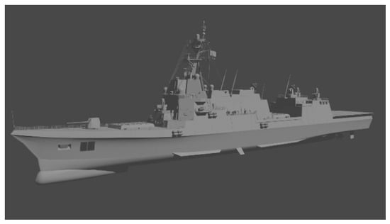
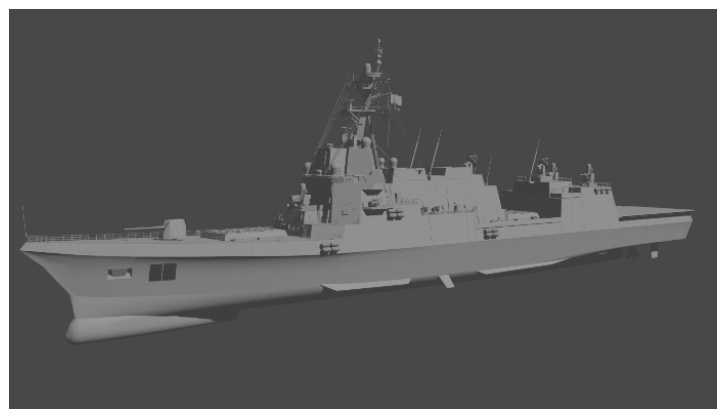
The ship model is an Arleigh Burke-class destroyer, taken here as a representative medium-sized naval target. Its three-dimensional CAD geometry is shown in Figure 1. The high-frequency electromagnetic response under the specified incidence and azimuth angles is computed with FEKO, and the resulting intrinsic polarimetric scattering matrix is projected onto the SAR image plane. The sea surface is generated from the Elfouhaily unified spectrum. Wind speeds between 3 and 12 m/s are used to control the sea state, and the two-scale model is employed to calculate the full-polarimetric backscattering field of the sea surface.

Figure 1. Three-dimensional structural model of the Arleigh Burke-class destroyer.

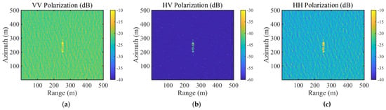
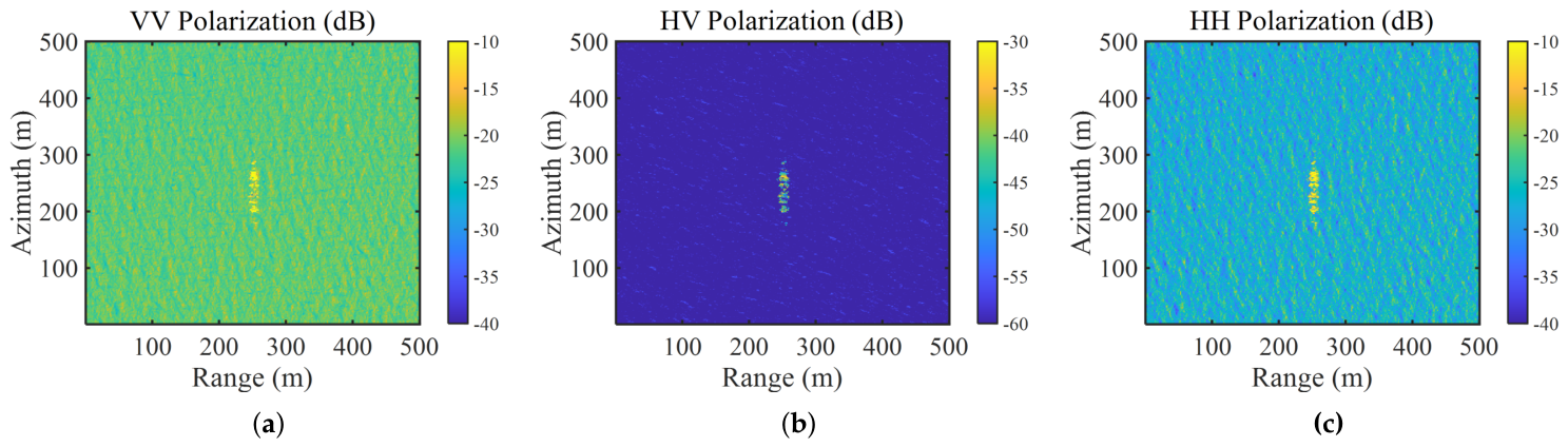
Figure 2 gives the Pol-SAR images of the reference scene without rainfall. The VV, HV, and HH channels show the expected scattering characteristics. The ship appears as several strong scattering centers, while the sea-surface background is mainly characterized by Bragg-scattering texture.

Figure 2. Sea-surface ship imaging results under clear-sky conditions. (a) VV Polarization. (b) HV Polarization. (c) HH Polarization.

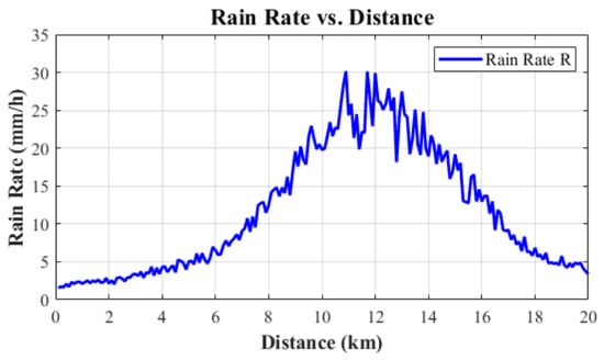
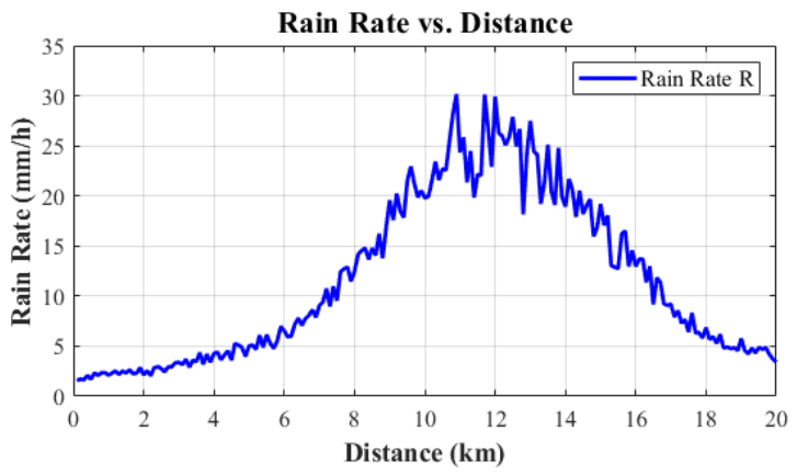
The rainfall field is generated with the hybrid rain–cell model [38,39], which produces a non-uniform rainfall-rate distribution. Its analytical form is given in Equation (26). Along the propagation path, the rain region is divided into N locally homogeneous cells, each 100 m long. The propagation matrix for each cell is calculated using the method in Section 2.2, and the overall propagation matrix is obtained by cascading the matrices of all cells. The hydrometeor volume-scattering model is also used to generate additive rain clutter in each cell. The sea-surface and ship echoes after propagation are then combined with the rain clutter to form the final polarimetric observations. Several comparison scenarios are constructed by changing the mean rainfall rate, the rain–cell parameters, and the sea-surface wind speed. A representative rainfall-rate profile along the propagation path is shown in Figure 3.

$$R(x,y)=\left\{\begin{array}{cc}{R}_{\mathrm{G}}exp\left[-\left({\displaystyle \frac{x^2}{a_{\mathrm{G}}^2}}+{\displaystyle \frac{y^2}{b_{\mathrm{G}}^2}}\right)\right],\hfill & R(x,y)\ge R_1,\hfill \\ R_{\mathrm{E}}exp\left[-{\left({\displaystyle \frac{x^2}{a_{\mathrm{E}}^2}}+{\displaystyle \frac{y^2}{b_{\mathrm{E}}^2}}\right)}^{1/2}\right],\hfill & R_2\le R(x,y)\le R_1.\hfill \end{array}\right.$$

(26)

where $R_{\mathrm{G}}$ is the maximum rainfall rate at the center of the rain cell. The parameters $a_{\mathrm{G}}$ and $b_{\mathrm{G}}$ are the scale parameters of the Gaussian component, and $a_{\mathrm{E}}$ and $b_{\mathrm{E}}$ are those of the exponential component. The Gaussian term describes the core rain region, whereas the exponential term describes the outer rain region.

Figure 3. Rainfall rate as a function of propagation distance.

The following subsections evaluate the effect of rainfall on Pol-SAR imaging and ship detection in the simulated scenes. The metrics are target SCNR and pixel-level detection probability $P_{\mathrm{d}}$. Reference methods are included for comparison.

4.2. Degradation Analysis of Pol-SAR Imaging Under Non-Uniform Rainfall

Non-uniform rain reduces image quality. Two terms cause the loss: propagation attenuation and rain clutter. The degradation level changes with rainfall rate, rain-field variation, propagation distance, and system SNR. These factors are not analyzed at once. We first study attenuation with a uniform-rain model. Then we use the non-uniform case to evaluate the final loss in imaging and detection.

4.2.1. Influence of Rainfall Rate Along the Propagation Path

In a non-uniform rainfall environment, attenuation along the propagation path builds up over range and appears as a reduction in signal amplitude and effective SNR. A uniform-rainfall model is adopted first so that this effect can be separated from additive rain clutter. Only the multiplicative effect introduced by the propagation matrix is retained, which makes it possible to study propagation attenuation on its own.

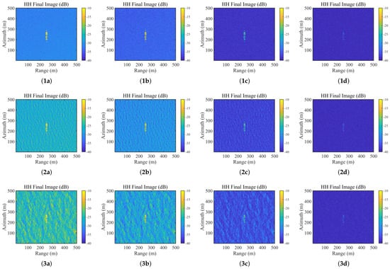
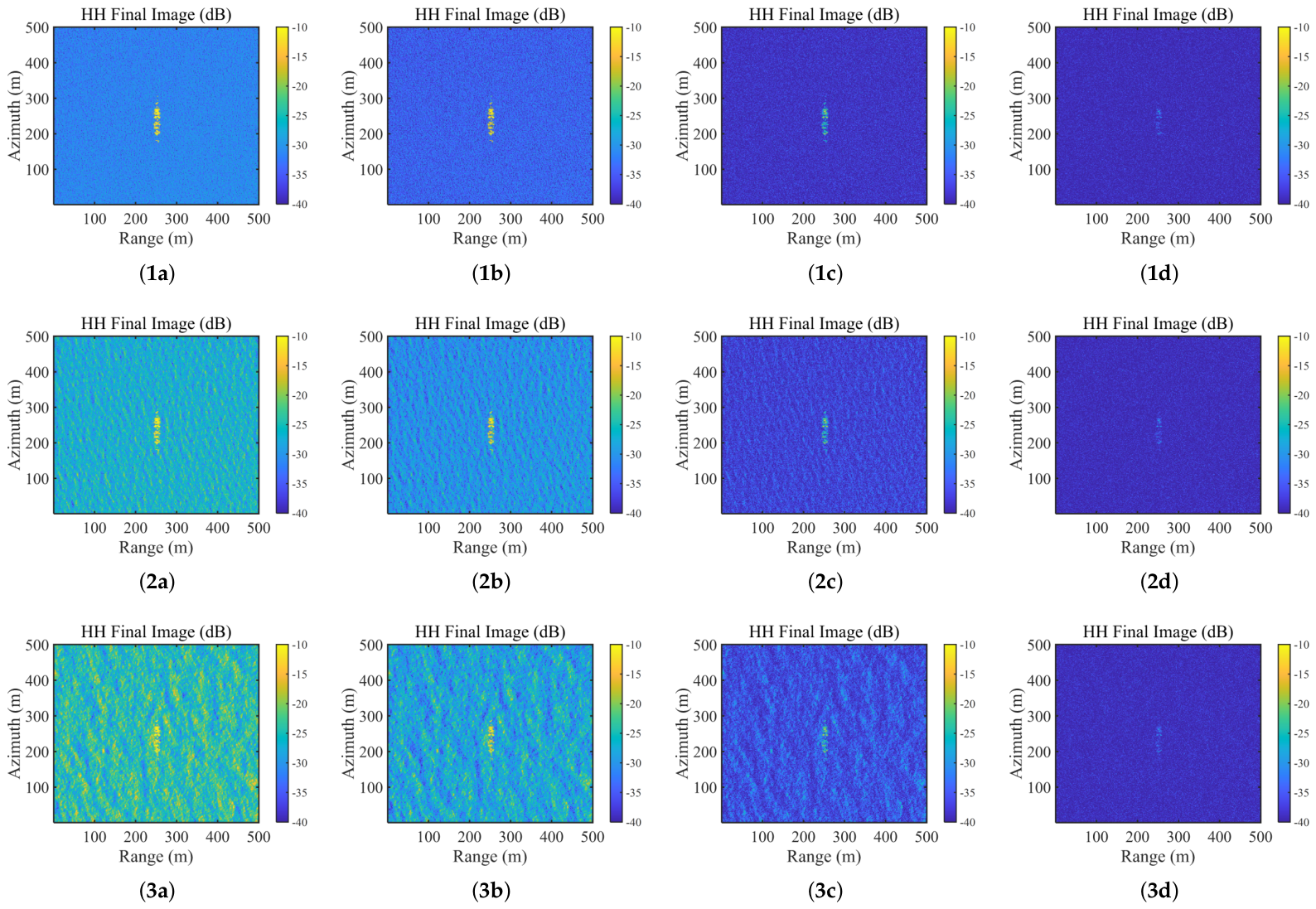
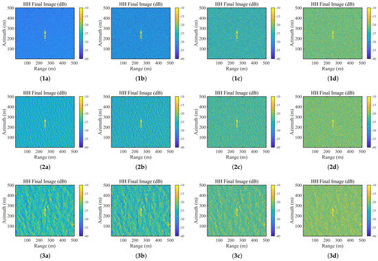
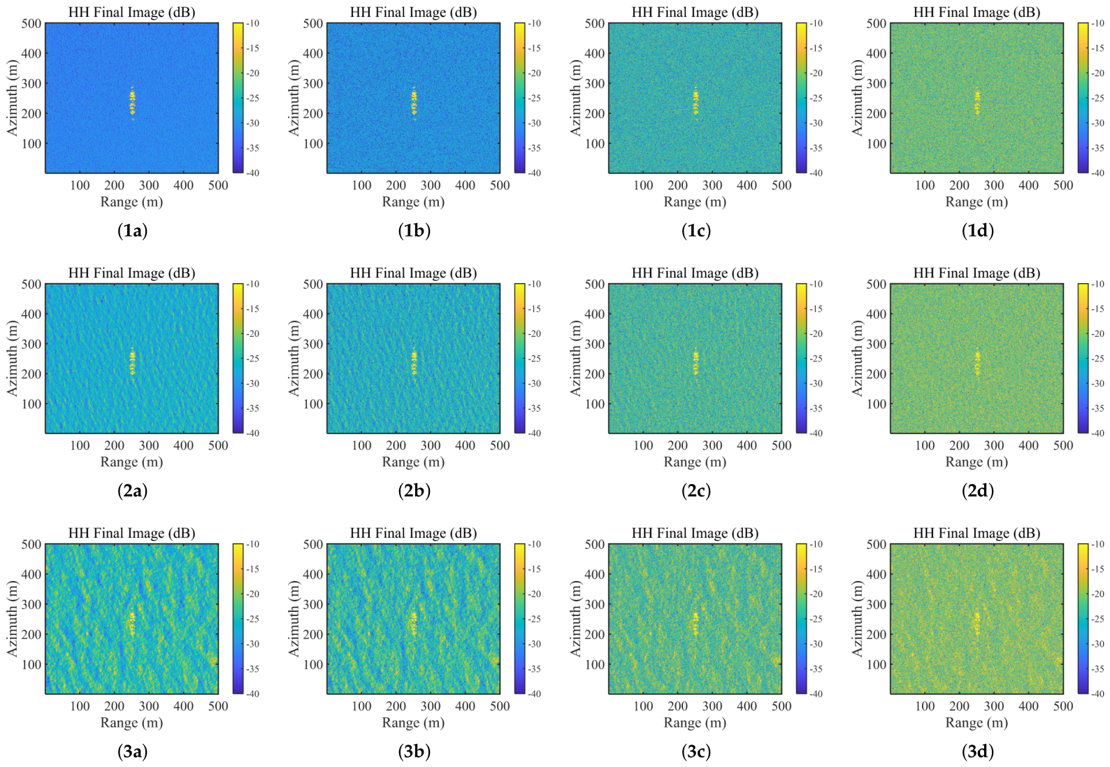
The rainfall rate is assumed constant along the propagation path in this experiment. Different attenuation levels are produced by changing the rainfall rate, while local rain-clutter scattering at the target cell is excluded. Figure 4 shows imaging results for different sea states and rainfall rates. As the uniform rainfall rate increases, the image becomes dimmer, and the amplitudes of both target and background are compressed. The target shape and spatial outline, however, remain largely unchanged, suggesting that propagation attenuation mainly rescales echo amplitude rather than distorting target structure.

Figure 4. Pol-SAR imaging comparison under varying rainfall rates and sea states (10 km propagation distance, 30 dB SNR). Groups (1), (2), and (3) correspond to wind speeds of 3, 8, and 12 m/s, respectively. Within each group, panels (a–d) correspond to rainfall rates of 0, 5, 12, and 20 mm/h.

The CA-CFAR detector is then applied with a fixed false alarm rate of $P_{\mathrm{fa}}={10}^{-3}$, and the resulting detection probabilities are listed in Table 3. Under low and moderate rainfall, the detection result changes only slightly even though the target echo weakens. At high rainfall rates, $P_{\mathrm{d}}$ drops quickly because attenuation lowers the SNR at the receiver.

Table 3. Detection probability $P_{\mathrm{d}}$ under varying uniform rainfall rates and sea states ($P_{\mathrm{fa}}={10}^{-3}$).

Rainfall Rate	Wind Speed 3 m/s	Wind Speed 8 m/s	Wind Speed 12 m/s
0 mm/h	0.89	0.72	0.57
5 mm/h	0.86	0.70	0.54
12 mm/h	0.71	0.58	0.47
20 mm/h	0.11	0.10	0.10

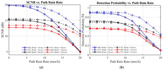
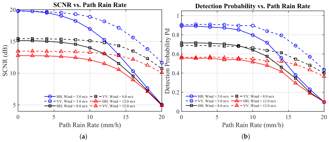
We evaluate SCNR and pixel-level detection probability $P_{\mathrm{d}}$ in the HH and VV channels against the mean rainfall rate along the propagation path, with $P_{\mathrm{fa}}={10}^{-3}$. Three sea states are used: wind speeds of 3, 8, and 12 m/s. The rainfall rate is varied from 0 to 20 mm/h. Each setting is run 20 times in Monte Carlo simulation. The results are shown in detail in Figure 5.

Figure 5. SCNR and pixel-level detection probability under uniform path rainfall. HH and VV channels are compared for path rainfall rates from 0 to 20 mm/h under sea-surface wind speeds of 3, 8, and 12 m/s, with $P_{\mathrm{fa}}={10}^{-3}$ and 20 Monte Carlo runs per setting. (a) SCNR versus path rainfall rate. (b) Detection probability $P_{\mathrm{d}}$ versus path rainfall rate.

In all three sea states, SCNR and detection probability decrease with rainfall rate in both HH and VV. The main reason is two-way attenuation of the target echo, which lowers target-to-background contrast. Compared with VV, the HH channel shows a larger SCNR loss across all sea states, and its detection probability decreases more noticeably in the medium- and high-rainfall ranges. HH polarization is therefore more sensitive to rain-induced attenuation. Rougher sea states further lower the clear-sky SCNR and detection probability, so the effect of rainfall becomes more evident once the sea clutter is already strong.

4.2.2. Influence of Local Rainfall Rate at the Target

In an actual rain field, the local rainfall rate at the target cell can differ from the mean rainfall rate along the propagation path. Unlike propagation attenuation, which acts multiplicatively, local rainfall at the target introduces additive rain clutter through hydrometeor volume scattering and directly changes the scattering statistics around the target. To isolate this effect, the mean rainfall rate along the propagation path is set to zero here, and only the local rainfall rate at the target cell is varied.

The local amplitude of the hybrid rain–cell model is adjusted to generate different rainfall intensities at the target cell, which gives a case containing only additive rain-clutter interference. Figure 6 shows representative imaging results. As the local rainfall rate increases, the background texture around the target becomes more complex, and the increase in clutter power weakens the contrast between the target and the background. Unlike the previous case, where the main effect was global amplitude compression and brightness reduction, the degradation here appears mainly as a local change in the statistical structure near the target.

Figure 6. Pol-SAR imaging comparison under varying local rainfall rates at the target cell, isolating the additive rain-clutter effect. The mean path rainfall rate is set to zero, the propagation distance is 10 km, and the input SNR is 30 dB. Groups (1), (2), and (3) correspond to wind speeds of 3, 8, and 12 m/s, respectively. Within each group, panels (a–d) correspond to local rainfall rates of 0, 5, 12, and 20 mm/h.

The CA-CFAR results in Table 4 are obtained under the same fixed false alarm rate. As the local rainfall rate increases, missed detections first appear in the medium-rainfall regime and become more frequent at higher rainfall levels, so the detection probability declines steadily. This case is different from the attenuation-driven one. Here, the probability does not fall abruptly. Additive rain clutter mainly raises local background power and changes nearby statistics. It does not directly weaken the target echo in a systematic way. The loss appears first as reduced local contrast, not as a sudden drop in global SNR.

Table 4. Detection probability $P_{\mathrm{d}}$ under varying local rainfall rates and sea states ($P_{\mathrm{fa}}={10}^{-3}$).

Rainfall Rate	Wind Speed 3 m/s	Wind Speed 8 m/s	Wind Speed 12 m/s
0 mm/h	0.89	0.72	0.57
5 mm/h	0.85	0.69	0.53
12 mm/h	0.58	0.48	0.40
20 mm/h	0.33	0.30	0.26

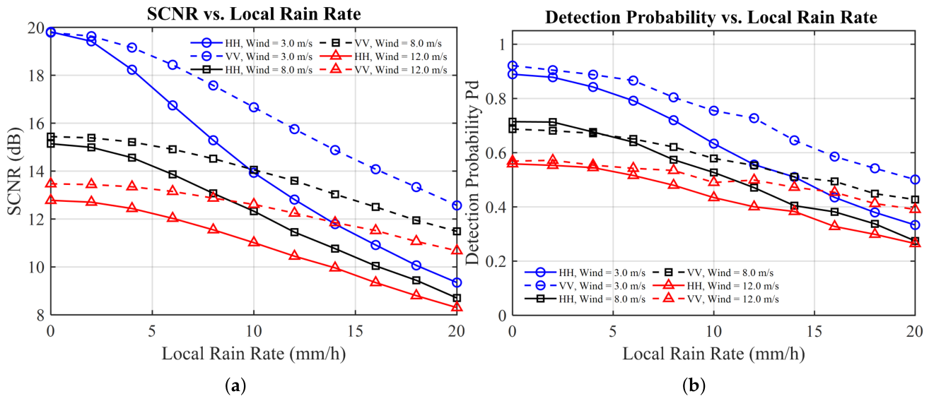
We also test the effect of rainfall at the target location. SCNR and pixel-level detection probability $P_{\mathrm{d}}$ are evaluated in the HH and VV channels against local rainfall rate, under the same false alarm setting. The same three sea states are used. The local rainfall rate varies from 0 to 20 mm/h. Each parameter set includes 20 Monte Carlo runs. The results are shown in Figure 7.

Figure 7. Influence of local rainfall rate at the target cell on SCNR and detection performance. With the mean path rainfall rate set to zero, the local rainfall rate is varied from 0 to 20 mm/h. HH and VV channels are compared under sea-surface wind speeds of 3, 8, and 12 m/s, with $P_{\mathrm{fa}}={10}^{-3}$ and 20 Monte Carlo runs per setting. (a) SCNR versus local rainfall rate. (b) Pixel-level detection probability $P_{\mathrm{d}}$ versus local rainfall rate.

The same trend is seen in all three sea states. In both channels, SCNR decreases almost linearly with local rainfall rate. The main source is the increase in background power from hydrometeor volume scattering. Ship-to-clutter contrast is then reduced. HH loses more SCNR than VV, and its detection probability falls faster. This shows higher HH sensitivity to local rain clutter. At medium and high rainfall rates, VV keeps the higher $P_{\mathrm{d}}$ and the steadier response.

4.2.3. Influence of Rain-Region Propagation Distance

In a non-uniform rain field, path length is another control variable. Propagation attenuation and rain-clutter power both depend on rainfall rate, through the per-unit-length propagation constant and the volume-scattering coefficient. The total effect also depends on the distance traveled inside the rain region. Attenuation follows coefficient × path length. Rain-clutter power follows the path integral of the unit-volume scattering term. At fixed rainfall rate, changing the path length changes multiplicative attenuation and additive rain clutter at the same time.

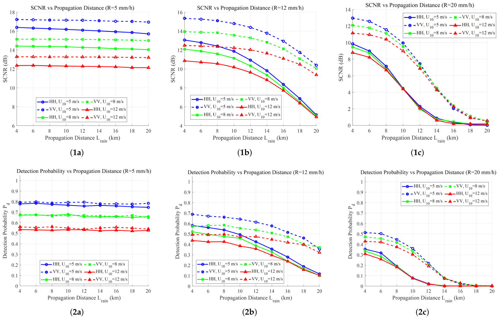
In this test, the sea state is fixed at $U_{10}=8$ m/s, and the rain-field pattern is unchanged. Three rainfall rates are used: 5, 12, and 20 mm/h. The rain region is taken as uniform, so the propagation attenuation and the local rain-clutter intensity stay consistent numerically. The effective path length in rain, $L_{\mathrm{rain}}$, is varied along the radar line of sight. SCNR and detection probability are then evaluated. In physical terms, this is equivalent to changing the target slant range or the rain-region extent. The corresponding SCNR and detection-probability curves are presented in Figure 8.

Figure 8. Influence of the effective propagation distance inside the rain region on imaging and detection performance in the HH and VV channels. The sea-surface wind speed is fixed at $U_{10}=8$ m/s, and the rain-region path length is varied from 4 km to 20 km. Columns (a–c) correspond to rainfall rates of 5, 12, and 20 mm/h, respectively. Row (1) reports SCNR, and row (2) reports pixel-level detection probability $P_{\mathrm{d}}$ at $P_{\mathrm{fa}}={10}^{-3}$.

The influence of propagation distance changes markedly with rainfall intensity. Under weak rainfall, SCNR and $P_{\mathrm{d}}$ in the HH and VV channels decrease slowly as $L_{\mathrm{rain}}$ increases from 4 km to 20 km. Under moderate rainfall, both SCNR and $P_{\mathrm{d}}$ decrease steadily with propagation distance, and the rate of degradation becomes larger at medium and long distances. Under strong rainfall, SCNR decreases rapidly as $L_{\mathrm{rain}}$ increases, and detection probability drops sharply once the propagation distance reaches the moderate range. The effect of propagation distance is therefore not simply linear. When rainfall is weak, changing the propagation distance has only a limited influence. Under moderate and strong rainfall, cumulative attenuation and rain-clutter accumulation reinforce each other, making detection performance much more sensitive to path length.

4.3. Simulation Analysis of Compensation and Enhancement Effects Under Non-Uniform Rainfall

The previous subsection treated propagation attenuation and local rain clutter separately through controlled experiments. Practical maritime scenes are less clean: non-uniform rainfall introduces cumulative attenuation along the propagation path together with hydrometeor volume scattering near the target. Under such conditions, a uniform-rainfall model is no longer sufficient. The composite scattering model in Section 2 is therefore used here to evaluate the propagation compensation and polarimetric zooming method introduced in Section 3.

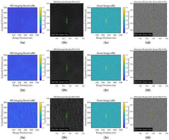
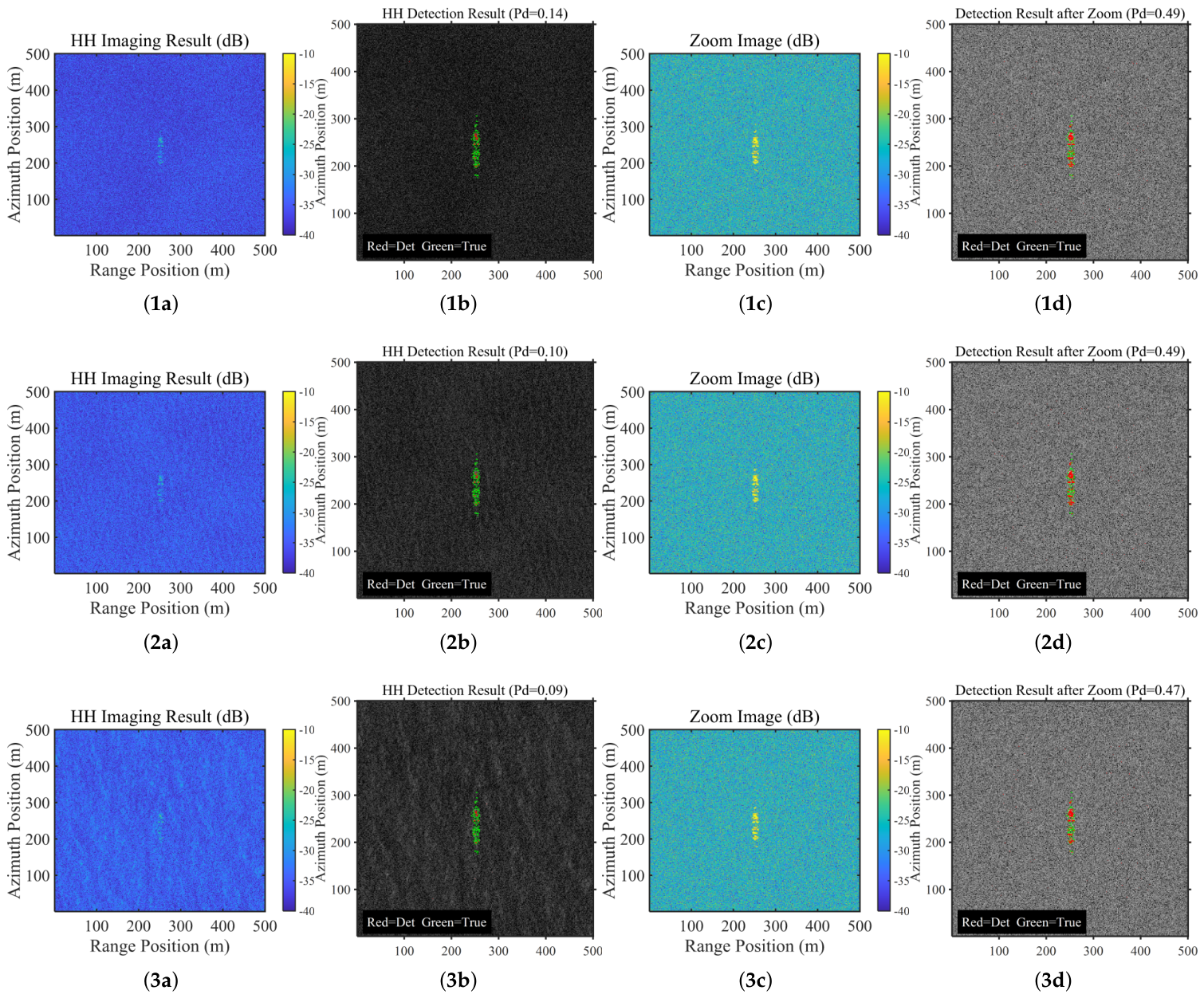
The simulation settings remain the same as those given above. The non-uniform rain field produces a rainfall-rate gradient along the radar line of sight, while the propagation distance is fixed at 10 km. For the representative case shown here, three outputs are compared: the uncompensated image, the image after propagation compensation and polarimetric zooming, and the corresponding detection result. A strong-rainfall case is selected as a representative challenging condition. Its peak rainfall rate is 24–30 mm/h, and the local rainfall rate at the target is 18–22 mm/h. Representative imaging and detection results are shown in Figure 9.

Figure 9. Visual comparison of Pol-SAR imaging and CA-CFAR detection before and after propagation compensation and polarimetric zooming under strong non-uniform rainfall. The peak rainfall rate is 24–30 mm/h, the local rainfall rate at the target is 18–22 mm/h, the propagation distance is 10 km, the input SNR is 30 dB, and $P_{\mathrm{fa}}={10}^{-3}$. Rows (1–3) correspond to wind speeds of 3, 8, and 12 m/s, respectively. Columns (a–d) correspond to the uncompensated HH image, detection without compensation, enhanced image after polarimetric zooming, and detection after enhancement, respectively.

Under strong non-uniform rainfall, the interference is heavier. In the uncompensated image, the target echo is attenuated, rain clutter gathers around the target, and stronger background fluctuations mask most of the ship structure. After propagation compensation and polarimetric zooming, part of the target energy returns. The ship outline becomes visible again. Some structural details can also be seen. The main target structure is still kept under strong rain cells and rough sea conditions.

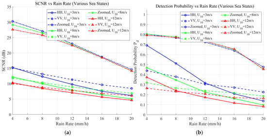
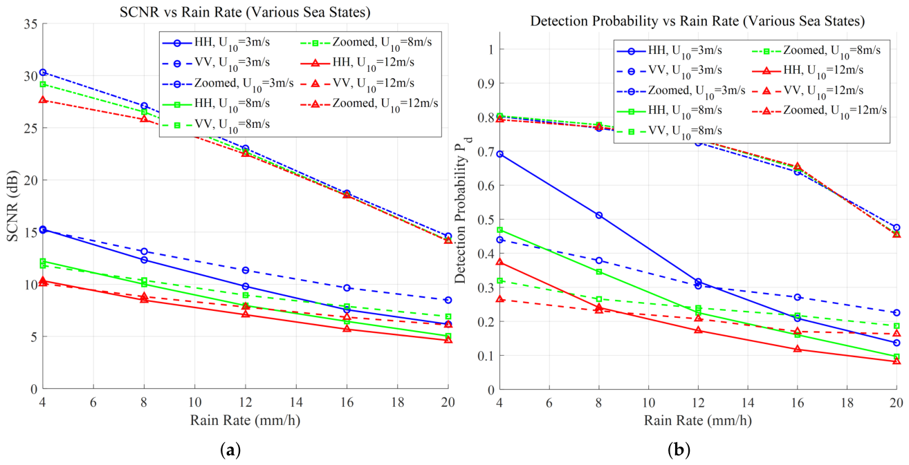
We evaluate the method statistically for different rain–cell peak intensities and for three sea states with wind speeds of 3, 8, and 12 m/s. For each setting, SCNR and pixel-level detection probability are estimated from 20 Monte Carlo runs at a fixed false alarm rate. The results are given in Figure 10.

Figure 10. Statistical comparison of single-channel imaging (HH, VV) and the proposed compensation-plus-zooming method (Zoom) under non-uniform rainfall, for rain–cell peak rainfall rates from 4 to 20 mm/h under sea-surface wind speeds of 3, 8, and 12 m/s, with $P_{\mathrm{fa}}={10}^{-3}$ and 20 Monte Carlo runs per setting. (a) SCNR comparison. (b) Pixel-level detection probability $P_{\mathrm{d}}$ comparison.

Among the single-polarization channels, VV performs slightly better than HH over all rainfall rates and sea states, although the difference is small under weak rainfall. As rainfall becomes stronger, the gap gradually becomes more evident. One reason is that hydrometeors are usually oblate, so horizontal polarization suffers stronger attenuation than vertical polarization, and the HH signal decreases faster along the propagation path. Hydrometeor backscatter can also be stronger in HH than in VV, which further increases the background level in HH. Accordingly, SCNR and $P_{\mathrm{d}}$ decrease faster in HH, whereas VV remains relatively more stable under moderate and strong rainfall.

Compared with the single-channel VV result, the proposed method provides a further improvement because it combines propagation compensation with receive-polarization optimization. In terms of SCNR, the enhanced result is higher than VV in all tested cases, with an improvement of about 6 to 15 dB. In a low-rainfall case at a wind speed of 3 m/s, SCNR increases from about 15 dB to about 30 dB, whereas at a rainfall rate of 20 mm/h it still increases from 8 dB to 14 dB. Detection performance changes in the same direction. Without enhancement, the detection performance of VV deteriorates as rainfall and sea state increase. Under the combined condition of 20 mm/h rainfall and a sea state of 12 m/s, $P_{\mathrm{d}}$ decreases to 0.16. After enhancement, $P_{\mathrm{d}}$ remains in the range of 0.71 to 0.81 under moderate rainfall and 0.45 to 0.65 under strong rainfall, corresponding to an average increase of 0.2 to 0.4 relative to VV. Although the gain becomes smaller as rainfall increases because propagation attenuation and noise amplification become stronger, the proposed method still improves target visibility under all tested conditions and reduces the loss in detection performance under coupled rainfall and sea clutter.

4.4. Comparison with Reference Polarimetric Detection Methods

The proposed method, denoted as Zoom, is compared here with five representative polarimetric reference methods. The first is the polarimetric whitening filter (PWF), which uses only the background covariance matrix and does not require prior target information. The second is the polarimetric matched filter (PMF), which assumes that both the target scattering signature and the covariance of the pure background are known; it is therefore treated as an oracle-style reference rather than a practical prior-free detector. To broaden the comparison, three additional prior-free polarimetric detectors are also included: the total polarimetric power (SPAN), defined as $|S_{\mathrm{HH}}{|}^2+2|S_{\mathrm{HV}}{|}^2+{\left|S_{\mathrm{VV}}\right|}^2$; the polarimetric notch filter (PNF) [15]; and a reflection-symmetry metric (RefSym) [14], none of which requires a target prior. Together with PWF, these constitute four prior-free baselines, whereas PMF serves as an oracle-style reference.

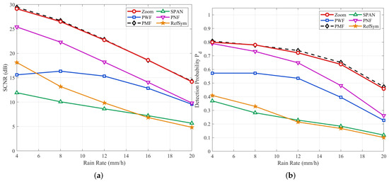
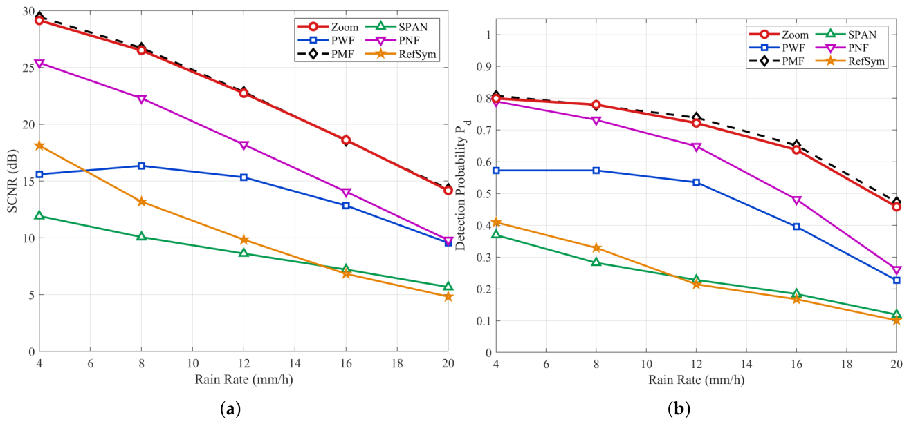
Zoom, PWF, PMF, SPAN, PNF, and RefSym are applied to the same simulated Pol-SAR observations generated under non-uniform rainfall. All six methods use the same CA-CFAR detector and the same fixed false alarm rate. Performance is evaluated by SCNR and detection probability $P_{\mathrm{d}}$. The simulation settings follow those in the previous subsection. For each combination of rain–cell peak intensity and sea state, the reported values are averaged over 20 Monte Carlo trials. The results are summarized in Figure 11.

Figure 11. Performance comparison of Zoom with five reference polarimetric methods under non-uniform rainfall: PWF, PMF, SPAN, PNF, and RefSym. All methods use the same CA-CFAR detector with $P_{\mathrm{fa}}={10}^{-3}$ and are evaluated at a representative sea state ($U_{10}=8$ m/s) for rain–cell peak rates from 4 to 20 mm/h. Each method is shown with a distinct color and marker, and each setting is averaged over 20 Monte Carlo runs. (a) SCNR. (b) Pixel-level detection probability $P_{\mathrm{d}}$.

For the representative sea state shown in Figure 11 ($U_{10}=8$ m/s), Zoom gives higher SCNR and $P_{\mathrm{d}}$ than PWF and remains close to the PMF oracle-style reference. All six methods degrade as rainfall increases, but the drop is smaller for Zoom. At low rainfall, the SCNR values of Zoom, PWF, and PMF are about 29.1, 15.6, and 29.5 dB, so Zoom is more than 13 dB above PWF; at 20 mm/h they become about 14.2, 9.6, and 14.3 dB, and the gain over PWF drops to about 4.6 dB. The gap becomes smaller at higher rainfall rates, but Zoom still keeps higher target contrast under mixed rain and sea clutter. Among the additional prior-free baselines, PNF is the closest competitor but remains several decibels below Zoom over the tested range, while SPAN and RefSym are markedly lower. Zoom therefore keeps the best target contrast among the tested prior-free detectors.

The detection results follow the same pattern. For the same representative sea state, $P_{\mathrm{d}}$ decreases from about 0.80 at low rainfall to about 0.46 at 20 mm/h for Zoom, while PWF falls from about 0.57 to about 0.23 over the same range. Among the prior-free baselines, PNF again ranks closest to Zoom and remains above PWF, while SPAN and RefSym give the lowest detection probabilities. The gap between Zoom and PMF is small under the present evaluation protocol: over all tested cases, the SCNR difference is within about 0.31 dB, and the detection-probability difference is within 0.03. This indicates that propagation compensation plus polarimetric zooming can approach the PMF reference without using an explicit target template.

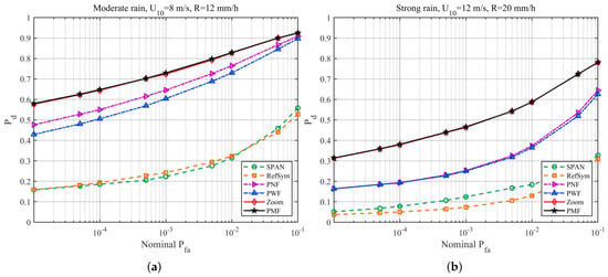
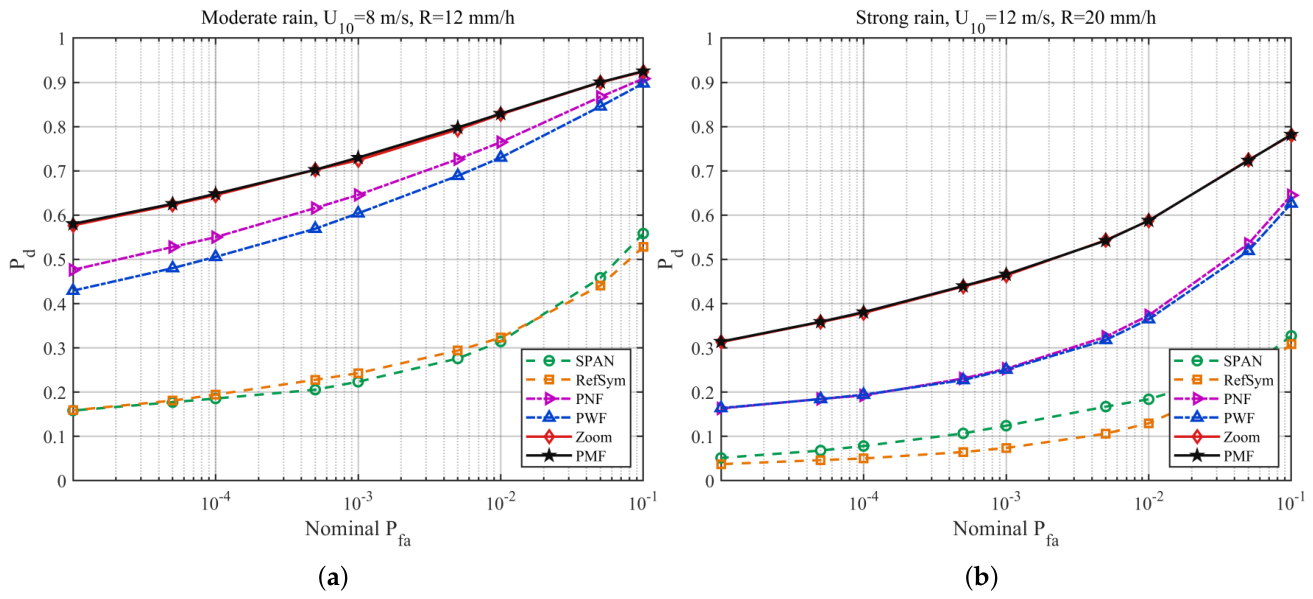
To complement the fixed-$P_{\mathrm{fa}}$ comparison in Figure 11, Figure 12 sweeps the nominal CA-CFAR false-alarm probability over $[{10}^{-5},{10}^{-1}]$ for the same six methods at a moderate condition $(U_{10},R)=(8\mathrm{m}/\mathrm{s},12\mathrm{mm}/\mathrm{h})$ and a harsh condition $(12\mathrm{m}/\mathrm{s},20\mathrm{mm}/\mathrm{h})$. Across the full $P_{\mathrm{fa}}$ range the method ordering is preserved, with the Zoom curve remaining closest to the PMF reference.

Figure 12. Receiver operating characteristic ($P_{\mathrm{d}}$ versus nominal $P_{\mathrm{fa}}$) of Zoom, PWF, PMF, SPAN, PNF, and RefSym under two representative non-uniform rainfall conditions. The nominal CA-CFAR false-alarm probability is swept over $[{10}^{-5},{10}^{-1}]$, and each setting is averaged over 20 Monte Carlo runs. (a) Moderate condition: $U_{10}=8$ m/s and $R=12$ mm/h. (b) Harsh condition: $U_{10}=12$ m/s and $R=20$ mm/h.

4.5. Error-Injection Sensitivity Analysis

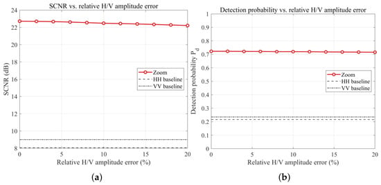
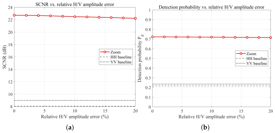
To assess the robustness of the recursive compensation stage, we perform an error-injection sensitivity analysis on the estimated H- and V-polarized propagation terms used for compensation. Controlled perturbations are applied to these terms and accumulate multiplicatively along the range direction, consistent with the cascaded structure of the propagation model. The perturbations are applied in relative H/V form because any common multiplicative error largely cancels in the HH-to-VV ratio used to initialize the receive-state search. The analysis is conducted under a representative non-uniform rainfall condition with $U_{10}=8$ m/s, rain–cell peak rate $R=12$ mm/h, and $P_{\mathrm{fa}}={10}^{-3}$. The relative H/V amplitude error is swept from 0 to 20%, and the one-way relative H/V phase error from $0^{\circ }$ to ${20}^{\circ }$, each varied separately.

Figure 13 shows that relative H/V amplitude perturbations have a limited effect in this test. When the relative amplitude error increases from 0 to 20%, SCNR decreases only from 22.72 to 22.22 dB, and $P_{\mathrm{d}}$ decreases from 0.722 to 0.715. Across the tested range, the Zoom result stays well above the HH and VV single-channel baselines, indicating that the proposed compensation is robust to a relative amplitude mismatch between the H- and V-polarized propagation terms.

Figure 13. Sensitivity to the relative H/V amplitude error under $U_{10}=8$ m/s, rain–cell peak rate $R=12$ mm/h, and $P_{\mathrm{fa}}={10}^{-3}$. Each point is averaged over 20 Monte Carlo runs. The dashed and dash-dotted lines show the HH and VV single-channel baselines. (a) SCNR. (b) Detection probability.

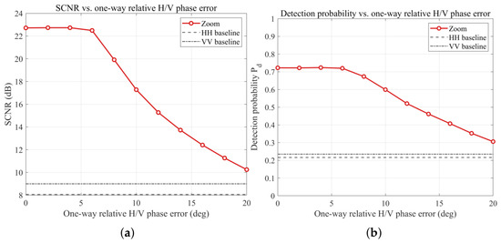
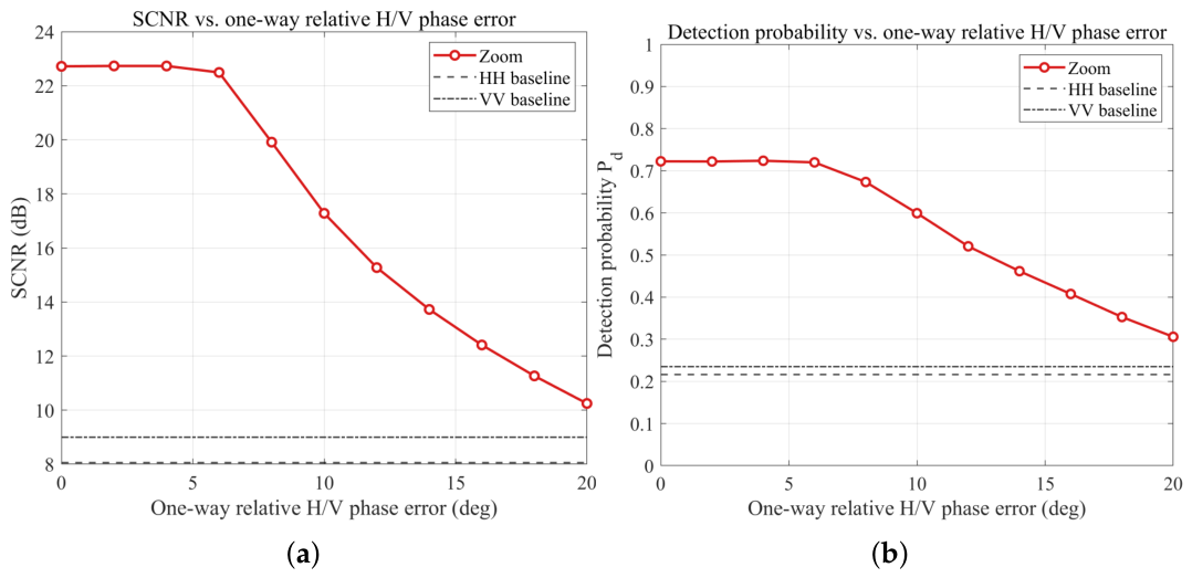
In contrast, Figure 14 shows that one-way relative H/V phase perturbations lead to more pronounced degradation. The relative phase error has a stronger effect because it changes the phase relationship between the H- and V-polarized propagation terms and can shift the estimated background polarization state. At a ${10}^{\circ }$ one-way relative phase error, SCNR decreases to 17.28 dB and $P_{\mathrm{d}}$ decreases to 0.599. Under a more severe ${20}^{\circ }$ error, SCNR remains 10.25 dB and $P_{\mathrm{d}}$ remains 0.306, still higher than the HH and VV single-channel baselines under the same condition.

Figure 14. Sensitivity to the one-way relative H/V phase error under $U_{10}=8$ m/s, rain–cell peak rate $R=12$ mm/h, and $P_{\mathrm{fa}}={10}^{-3}$. Each point is averaged over 20 Monte Carlo runs. The dashed and dash-dotted lines show the HH and VV single-channel baselines. (a) SCNR. (b) Detection probability.

The sensitivity results indicate that a residual error in the compensating propagation terms influences the proposed method mainly through phase-dependent polarization mismatch. The SCNR and detection-probability losses remain limited when the injected one-way relative H/V phase error is within $5^{\circ }$, whereas larger errors of ${10}^{\circ }$ or above lead to more visible degradation. This trend indicates that phase consistency between the H- and V-polarized propagation terms is more critical than a small relative amplitude mismatch. In the present recursive scheme, one concrete source of such a residual error is the starting assumption that propagation in the first range cell is negligible, which leaves a small uncompensated rain-induced term at the recursion origin. This term is far below the tested range: a first range cell of length 100 m with a residual rainfall rate of 20 mm/h introduces a one-way relative H/V phase shift of approximately $0.{16}^{\circ }$ and a relative H/V amplitude mismatch below $0.2\%$, more than one order of magnitude below the lowest nonzero perturbation level used in the sweep. This comparison supports the assumption that rain-induced propagation in the first range cell is negligible within the propagation-model setting considered here.

5. Discussion

The degradation is coupled. Non-uniform rainfall affects Pol-SAR sea-target detection through propagation distortion and background contamination. These two terms interact, reducing target visibility and making the local background less stable under changing rainfall and sea-state conditions. The results in Section 4 suggest that detection in rainy maritime scenes benefits from jointly considering propagation correction and rain-clutter suppression.

The comparison with the reference methods shows that the main benefit of the proposed framework lies in reducing rain-induced background non-stationarity before polarimetric detection. PWF relies only on the estimated background covariance matrix and is therefore more sensitive to spatially varying rain clutter and rough-sea fluctuations. In contrast, the proposed framework first compensates for propagation distortion and then performs receive-polarization optimization on the compensated polarimetric response. The small gap between Zoom and the PMF oracle-style reference reflects the controlled test protocol and the oracle nature of PMF, which assumes target and pure-background prior information that is generally unavailable in practical scenes.

This study has several limitations. The rain-field, sea-surface, and target-scattering models remain simpler than real maritime scenes. Real observations can include stronger spatial and temporal rain variation, ship motion, wakes, stronger sea-surface non-stationarity, calibration errors, channel imbalance, and non-ideal receiver noise. The error-injection analysis in Section 4.5 characterizes the influence of initial propagation-matrix estimation errors, and future validation using field observation data under known rainfall conditions will further assess practical performance. Future work will focus on validation using field observation data, more heterogeneous rain fields, and more robust parameter-retrieval, polarization-optimization, and detection schemes.

6. Conclusions

This study investigates Pol-SAR imaging and ship detection over the sea surface under non-uniform rainfall using a physics-based framework. A composite polarimetric scattering model is established for the coupled rain region, sea surface, and ship target, enabling pathwise propagation distortion and local rain clutter to be analyzed within a unified setting. Based on this framework, a joint method combining propagation compensation and polarimetric zooming is proposed. Under the tested conditions, the proposed method reduces rain-induced degradation: compared with PWF, it improves SCNR by about 4 to 13 dB and increases detection probability by about 0.23 at the representative sea state across the tested rainfall rates. Moreover, its performance remains close to the PMF oracle-style reference, with SCNR differences generally within about 0.31 dB and detection-probability differences mostly within about 0.03, while avoiding the need for an explicit target template.

The error-injection results provide a representative sensitivity assessment of the recursive initialization assumption. Future work will validate the proposed framework using field observation data under known rainfall conditions.

References

- Cumming, I.G.; Wong, F.H. Digital Processing of Synthetic Aperture Radar Data: Algorithms and Implementation; Artech House: Norwood, MA, USA, 2005. [Google Scholar]
- Cloude, S.R.; Pottier, E. An entropy based classification scheme for land applications of polarimetric SAR. IEEE Trans. Geosci. Remote Sens. 1997, 35, 68–78. [Google Scholar] [CrossRef] [Scilit]
- Lee, J.-S.; Pottier, E. Polarimetric Radar Imaging: From Basics to Applications; CRC Press: Boca Raton, FL, USA, 2009. [Google Scholar]
- Zhang, C.; Gao, G.; Zhang, X.; Li, H.-C.; Liu, T.; Zhang, Z.; Li, G. An overview of polarized synthetic aperture radar ship detection: From traditional methods to artificial intelligence. IEEE Geosci. Remote Sens. Mag. 2025, 13, 174–209. [Google Scholar] [CrossRef] [Scilit]
- Crisp, D.J. The State-of-the-Art in Ship Detection in Synthetic Aperture Radar Imagery; DSTO-RR-0272; DSTO Information Sciences Laboratory: Edinburgh, Australia, 2004. [Google Scholar]
- Perry, R.P.; DiPietro, R.C.; Fante, R.L. SAR imaging of moving targets. IEEE Trans. Aerosp. Electron. Syst. 1999, 35, 188–200. [Google Scholar] [CrossRef] [Scilit]
- Park, H.R.; Li, J.; Wang, H. Polarization-space-time domain generalized likelihood ratio detection of radar targets. Signal Process. 1995, 41, 153–164. [Google Scholar] [CrossRef] [Scilit]
- Wang, G.; Xia, X.; Chen, V.C. Radar imaging of moving targets in foliage using multifrequency multiaperture polarimetric SAR. IEEE Trans. Geosci. Remote Sens. 2003, 41, 1755–1764. [Google Scholar] [CrossRef] [Scilit]
- Kirscht, M. Detection and velocity estimation of moving objects in a sequence of single-look SAR images. In Proceedings of the 1996 International Geoscience and Remote Sensing Symposium (IGARSS); University of Nebraska: Lincoln, NE, USA, 1996; pp. 333–335. [Google Scholar]
- Zhang, P.; Zhang, J.; Liu, T. Slow and small target CFAR detection of polarimetric along-track interferometric SAR using coherence optimization. J. Beijing Univ. Aeronaut. Astronaut. 2019, 45, 575–587. [Google Scholar] [CrossRef]
- Zhang, P.; Zhang, J.; Liu, T. Contrastive analysis of the performances of radar multi-look polarimetric detectors. Chin. J. Radio Sci. 2017, 32, 416–426. [Google Scholar] [CrossRef]
- Boerner, W.M.; Kostinski, A.B.; James, B.D. On the concept of the polarimetric matched filter in high resolution radar imaging: An alternative for speckle reduction. In Proceedings of the International Geoscience and Remote Sensing Symposium, Remote Sensing: Moving Toward the 21st Century; IEEE: Edinburgh, UK, 1988; pp. 69–72. [Google Scholar]
- Novak, L.M.; Burl, M.C. Optimal speckle reduction in polarimetric SAR imagery. IEEE Trans. Aerosp. Electron. Syst. 1990, 26, 293–305. [Google Scholar] [CrossRef] [Scilit]
- Nunziata, F.; Migliaccio, M.; Brown, C.E. Reflection symmetry for polarimetric observation of man-made metallic targets at sea. IEEE J. Ocean. Eng. 2012, 37, 384–394. [Google Scholar] [CrossRef] [Scilit]
- Marino, A. A notch filter for ship detection with polarimetric SAR data. IEEE J. Sel. Top. Appl. Earth Obs. Remote Sens. 2013, 6, 1219–1232. [Google Scholar] [CrossRef] [Scilit]
- Gao, G.; Gao, S.; He, J.; Li, G. Ship detection using compact polarimetric SAR based on the notch filter. IEEE Trans. Geosci. Remote Sens. 2018, 56, 5380–5393. [Google Scholar] [CrossRef]
- Yang, J.; Yamaguchi, Y.; Boerner, W.-M.; Lin, S. Numerical methods for solving the optimal problem of contrast enhancement. IEEE Trans. Geosci. Remote Sens. 2000, 38, 965–971. [Google Scholar] [CrossRef]
- Yang, D.; Du, L.; Liu, H.; Ni, W. Novel polarimetric contrast enhancement method based on minimal clutter to signal ratio subspace. IEEE Trans. Geosci. Remote Sens. 2019, 57, 8570–8583. [Google Scholar] [CrossRef]
- Bordbari, R.; Maghsoudi, Y. A new target detector based on subspace projections using polarimetric SAR data. IEEE Trans. Geosci. Remote Sens. 2019, 57, 3025–3039. [Google Scholar]
- Deng, R.; Zhang, T.; Xu, X.; Zhang, X.; Gao, G. Tri-State Prototype Self-Distillation for SAR Ocean Imagery Panoptic Segmentation. IEEE Geosci. Remote Sens. Lett. 2026. early access. [Google Scholar] [CrossRef] [Scilit]
- Zhang, T.; Zhang, X.; Gao, G. Density Knowledge Mining for Quantity-Aware Marine Vessel Surveillance Using Satellite SAR Data. IEEE Trans. Ind. Inform. 2026. early access. [Google Scholar] [CrossRef] [Scilit]
- Zhang, T.; Gao, G.; Zhang, X. Triple-Level Sparsity Awareness for Marine Ship Surveillance Using Satellite Synthetic Aperture Radar. IEEE Trans. Autom. Sci. Eng. 2026, 23, 5155–5166. [Google Scholar] [CrossRef] [Scilit]
- Zhang, T.; Gao, G.; Ke, X.; Zhang, X. Swarm Learning: Perception–Retrieval–Localization for Ship Detection From Synthetic Aperture Radar Remote Sensing Imagery. IEEE J. Sel. Top. Appl. Earth Obs. Remote Sens. 2026. early access. [Google Scholar] [CrossRef] [Scilit]
- Danklmayer, A.; Döring, B.J.; Schwerdt, M.; Chandra, M. Assessment of atmospheric propagation effects in SAR images. IEEE Trans. Geosci. Remote Sens. 2009, 47, 3507–3518. [Google Scholar] [CrossRef]
- Alpers, W.; Zhang, B.; Mouche, A.; Zeng, K.; Chan, P.W. Rain footprints on C-band synthetic aperture radar images of the ocean revisited. Remote Sens. Environ. 2016, 187, 169–185. [Google Scholar] [CrossRef] [Scilit]
- Zhao, X.; Zhang, B.; Oruba, L.; Mouche, A.; Hauser, D. Effects of rain on the ocean radar backscatter at near-nadir incidence angles: Insights from the Ku-band SWIM/CFOSAT under low to strong wind observations. IEEE Trans. Geosci. Remote Sens. 2025, 63, 5106320. [Google Scholar] [CrossRef] [Scilit]
- Tian, Y.; Dong, X.-C.; Hu, C. Analysis of troposphere impacts on geosynchronous SAR imaging. J. Signal Process. 2015, 31, 1562–1567. [Google Scholar]
- Cong, X.; Balss, U.; Rodriguez Gonzalez, F.; Eineder, M. Mitigation of tropospheric delay in SAR and InSAR using NWP data: Its validation and application examples. Remote Sens. 2018, 10, 1515. [Google Scholar] [CrossRef] [Scilit]
- Wang, L.; Sun, L.; Gong, R.; Zhu, D. Error analysis in SAR imaging due to fluctuation of atmospheric refractive index. J. Electron. Inf. Technol. 2021, 43, 665–673. [Google Scholar]
- Zhou, H.; Dai, K.; Pirasteh, S.; Li, R.; Xiang, J.; Li, Z. InSAR spatial-heterogeneity tropospheric delay correction in steep mountainous areas based on deep learning for landslides monitoring. IEEE Trans. Geosci. Remote Sens. 2023, 61, 5215014. [Google Scholar] [CrossRef] [Scilit]
- Ju, X.; Li, X.; Gan, L.; Yin, J.; Shen, C.; Li, J. Impact and compensation of rainfall propagation effect on Pol-ISAR imaging of parabolic antenna. Remote Sens. 2025, 17, 855. [Google Scholar] [CrossRef] [Scilit]
- Mishchenko, M.I.; Travis, L.D.; Mackowski, D.W. T-matrix computations of light scattering by nonspherical particles: A review. J. Quant. Spectrosc. Radiat. Transf. 1996, 55, 535–575. [Google Scholar] [CrossRef] [Scilit]
- Testud, J.; Oury, S.; Black, R.A.; Amayenc, P.; Dou, X. The concept of normalized distribution to describe raindrop spectra: A tool for cloud physics and cloud remote sensing. J. Appl. Meteorol. 2001, 40, 1118–1140. [Google Scholar]
- Bringi, V.N.; Chandrasekar, V. Polarimetric Doppler Weather Radar: Principles and Applications; Cambridge University Press: Cambridge, UK, 2001. [Google Scholar]
- Elfouhaily, T.; Chapron, B.; Katsaros, K.; Vandemark, D. A unified directional spectrum for long and short wind-driven waves. J. Geophys. Res. Ocean. 1997, 102, 15781–15796. [Google Scholar] [CrossRef] [Scilit]
- Valenzuela, G.R. Theories for the interaction of electromagnetic and oceanic waves—A review. Bound.-Layer Meteorol. 1978, 13, 61–85. [Google Scholar] [CrossRef] [Scilit]
- Gordon, W.B. Far-field approximations to the Kirchhoff-Helmholtz representations of scattered fields. IEEE Trans. Antennas Propag. 1975, 23, 590–592. [Google Scholar] [CrossRef] [Scilit]
- Féral, L.; Sauvageot, H.; Castanet, L.; Lemorton, J. HYCELL—A new hybrid model of the rain horizontal distribution for propagation studies: 1. Modeling of the rain cell. Radio Sci. 2003, 38, 22-1–22-20. [Google Scholar] [CrossRef] [Scilit]
- Féral, L.; Sauvageot, H.; Castanet, L.; Lemorton, J. HYCELL—A new hybrid model of the rain horizontal distribution for propagation studies: 2. Statistical modeling of the rain rate field. Radio Sci. 2003, 38, 23-1–23-18. [Google Scholar] [CrossRef] [Scilit]
Disclaimer/Publisher’s Note: The statements, opinions and data contained in all publications are solely those of the individual author(s) and contributor(s) and not of MDPI and/or the editor(s). MDPI and/or the editor(s) disclaim responsibility for any injury to people or property resulting from any ideas, methods, instructions or products referred to in the content. |
© 2026 by the authors. Licensee MDPI, Basel, Switzerland. This article is an open access article distributed under the terms and conditions of the Creative Commons Attribution (CC BY) license.