Integrating Machine Learning with Adaptive Kalman Filtering to Downscale GFS Air Temperature Forecasts in Mountainous Areas

Highlights

What are the main findings?

• By employing a random forest statistical downscaling method from a geographical perspective, the DOWN step effectively refines the spatial detail of GFS air temperature distribution from a 0.25° resolution to 30 m.
• The bias correction (BC) step, using a first-order adaptive Kalman filter, substantially enhances air temperature forecast accuracy by achieving a reduction of over 30.0% in root mean square error compared to raw GFS forecasts.

What are the implications of the main findings?

• Air temperature forecasts are typically based on numerical weather prediction from an atmospheric science perspective. In contrast, forecasts with higher spatial resolution within mountainous areas must account for the effects of the underlying land surface.
• The proposed DOWN + BC method can also be applied to the latest GFS operational forecasts, which provide temperature data at 1 h resolution for the first 120 h and 3 h resolution from days 5 to 16. Furthermore, the DOWN + BC method holds practical potential for enhancing the spatial resolution of temperature distributions from other numerical weather prediction models.

Abstract

Accurate, high-resolution gridded air temperature forecasts are essential, particularly in mountainous areas with complex terrain. This study proposes a two-stage processing framework DOWN + BC to downscale Global Forecast System (GFS) temperature forecasts and correct their bias. The approach first employs a random forest (RF) model to geographically downscale 3-hourly 0.25° GFS forecasts to a 30 m resolution (DOWN), followed by bias correction (BC) using a first-order adaptive Kalman filter (AKF). The accuracy of the DOWN + BC-processed forecasts was evaluated against both automatic weather station (AWS) observations and high-resolution air temperature fields derived from an extreme gradient boosting model (XGB-derived). The results indicate that (1) the DOWN step effectively refines the spatial detail of temperature distribution, though it yields limited improvement in accuracy compared to the raw GFS forecasts; (2) the combined DOWN + BC method substantially enhances forecast accuracy. At AWS locations, the root mean square error (RMSE) of GFS forecasts decreased by 37.84% in January 2020 and 41.16% in July 2023. Relative to the XGB-derived temperature distribution, RMSE was reduced by 47.27% and 33.79% for the respective periods.

1. Introduction

Fine-resolution, hourly air temperature forecasts are essential for accurately modeling a wide range of physical processes [1,2], with significant implications across sectors such as agriculture, industry, transport, and sports. Accurate temperature prediction plays a key role in mitigating the impacts of extreme heat and cold on public health, preventing frost damage to crops and fruit [3], reducing mortality in aquaculture, lowering the incidence of winter road accidents due to icy conditions, and supporting logistics and safety for major sporting events. For instance, during the 2022 Beijing Winter Olympics, precise temperature forecasts tailored to specific competition tracks were critical for ensuring athlete performance and safety in snow sports. Therefore, producing accurate air temperature forecasts with high spatial and temporal resolution remains a priority for operational and applied needs.

Complex landscapes, variable topography, and sharp elevation changes over short distances strongly influence local weather patterns. In mountainous regions, high-resolution air temperature forecasts are therefore essential for both regional climate studies and human activities. The spatial and temporal distribution of air temperature in these areas is shaped not only by large-scale atmospheric circulation but also by local topographic factors such as altitude, slope, aspect, and shading. Subsurface conditions, including bedrock type and properties, also play a notable role [4]. Air temperature can vary markedly over small distances, for instance, mean annual temperature differences of up to 6 °C have been recorded within 1 km² areas in Northern Europe [5]. Ignoring such microclimatic variability can lead to substantial errors in research and practical applications [6]. A tragic example is the Gansu Mountain Marathon in Baiyin City on 22 May 2021, where inaccurate air temperature forecasting contributed to a severe public safety incident during the 100 km cross-country race, resulting in 21 fatalities. This underscores the critical need for reliable, high-resolution air temperature prediction in complex terrain.

Currently, a variety of numerical weather prediction (NWP) models are employed for air temperature forecasting [7]. However, these models face inherent challenges, including difficulties in parameterization and unavoidable errors in initial conditions [8], which often reduce forecast accuracy. Furthermore, most NWP models operate at grid spacings coarser than 1 km [9]. This limited spatial resolution makes it difficult to accurately represent and predict local-scale temperature variability, particularly in mountainous or topographically complex regions [10].

To achieve fine-resolution air temperature forecasts, researchers have developed both dynamical and statistical downscaling approaches. Dynamical downscaling incorporates physical mechanisms by nesting high-resolution regional climate models within coarse-resolution global models, thereby refining meteorological outputs [11]. However, this method is computationally intensive, often limiting practical grid resolutions to above 1 km, and it is susceptible to error propagation from the driving global model, necessitating bias correction through postprocessing [12,13]. In contrast, statistical downscaling establishes empirical relationships between large-scale model outputs and local observations to obtain finer-scale results. It is computationally efficient, easier to implement, and particularly suited for localized applications [14,15]. Many studies have employed machine learning algorithms to estimate air temperature, using remotely sensed variables—such as albedo, NDVI (Normalized Difference Vegetation Index), land-surface temperature, DEM (Digital Elevation Model), slope, and aspect—as predictors [7,16]. For example, Colaninno and Morello (2022) compared five machine learning models to estimate daily mean and instantaneous air temperature in the Jingjinji region of China using MODIS (the Moderate Resolution Imaging Spectroradiometer) land-surface temperature data, finding that the random forest (RF) algorithm outperformed the others [17]. Similarly, Zhang and Du (2022b) derived daily mean, maximum, and minimum temperatures by modeling scale-invariant relationships between temperature and remote sensing indices and topographic parameters [18]. Although these methods enable temperature estimation, their spatial and temporal resolution often remains limited. Currently, few approaches successfully deliver air temperature forecasts that simultaneously achieve high spatiotemporal resolution and high accuracy.

While continuous development in NWP models has led to notable improvements in forecast skill, initial conditions, and ensemble design [19], significant biases remain due to atmospheric nonlinearity and model error, especially in complex terrain [20]. Consequently, the accuracy of downscaled forecasts cannot be substantially improved without effective postprocessing. Kalman filtering offers an efficient approach for such grid-point bias correction [21]. The adaptive Kalman filter error correction method, which is also recursive and capable of real-time correction, has been successfully applied in ensemble prediction of minimum and maximum daily air temperatures and in error correction of large-scale model systems. This method relies on observations for calibration and employs weighted averaging to optimize state estimates, yielding enhanced forecast accuracy [22].

In summary, generating accurate air temperature forecasts at fine grid spacings, particularly over complex mountainous areas, represents an ongoing research need. The GFS serves as a foundational global model, typically run at 0.25° and 0.5° resolution for forecasts ranging from one to two weeks, and often provides initial and boundary conditions for regional models. Enhancing the resolution of its key outputs, such as air temperature at the height of 2 m, could yield operationally valuable, high-resolution meteorological fields for mountainous applications.

Based on numerical weather prediction from an atmospheric science perspective, this study adopts a geographical viewpoint to investigate downscaling techniques and error correction for GFS model predicted air temperatures, emphasizing the influence of multiple land-surface factors on air temperature variations. The research proposed the DOWN + BC method, a two-stage processing framework, which combines machine learning and an adaptive Kalman filter (AKF) to downscale and bias-correct GFS temperature forecasts, yielding high-precision 24 h forecasts at a 30 m grid spacing. The performance of this method was evaluated using 3-hourly 0.25° gridded GFS forecasts from January 2020 and July 2023.

2. Materials and Methods

2.1. Study Area

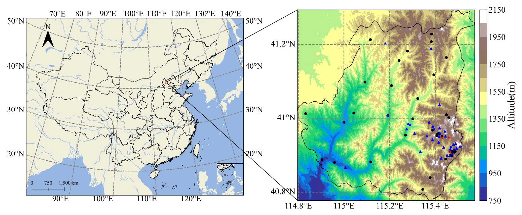
The study area, situated in Chongli District, Zhangjiakou City, Hebei Province, China (Figure 1), spans an area of 2300 km². Its coordinates range from 114.8° to 115.6° E longitude and 40.8° to 41.3° N latitude, occurring within the semiarid monsoon climate zone. The topography of Chongli District is diverse and comprises mountains, hills, valleys, and basins, with elevations ranging from 812 to 2169 m and an average altitude of 1485 m. These geographical features result in pronounced air temperature variations across the region. In January, Chongli experiences severe cold with pronounced spatial and temporal variability. Spatially, air temperatures decrease with elevation, ranging from about −11 °C in valleys to −17 °C at altitudes above 1500 m. The diurnal temperature range typically reaches 15 °C, and air temperature inversions frequently occur in valley bottoms during clear, calm nights, intensifying cold extremes in low-lying areas. In July, by contrast, air temperatures decrease from southwest to northeast as elevation increases, ranging from approximately 27 °C in valleys to notably cooler conditions at higher altitudes. The average high and low temperatures are around 27 °C and 15 °C in July, respectively.

Figure 1. Map of the location of the study area (the figure on the right shows the elevation of the study area, and the black dots indicate the AWS sites used in both January 2020 and July 2023; the triangles indicate the AWS sites only used in January 2020, and the stars indicate the AWS sites only used in July 2023).

2.2. Data

2.2.1. GFS Air Temperature Forecast Data

The Global Forecast System (GFS), developed by the National Centers for Environmental Prediction (NCEP), is a widely used weather forecasting model that generates global predictions for a wide range of atmospheric and land-surface variables, including temperature and precipitation. The system couples four separate models that work together to accurately depict weather conditions. This study selected the NCEP GFS 0.25° Global Forecast Grids Historical Archive dataset to evaluate the proposed DOWN + BC method. This dataset provides global forecast output at a spatial resolution of 0.25° and is updated four times daily (00, 06, 12, and 18 UTC). Forecasts are available at 3 h intervals out to a maximum lead time of 384 h. For the evaluation, we extracted 24 and 27 h temperature forecast fields from each of the four initialization times during January 2020 and July 2023. By combining these, we constructed a continuous 3-hourly temperature forecast series for each day (00, 03, 06, 09, 12, 15, 18, and 21 UTC), which was used to assess the accuracy and operational feasibility of the DOWN + BC method. For brevity in subsequent sections, dates are abbreviated as follows: D7 refers to 7 January 2020, J7 to 7 July 2023, and so forth.

2.2.2. Ground Observation Data

We utilized hourly air temperature observations at 2 m above ground level obtained from 73 automatic weather stations (AWSs) in January 2020 and 42 AWSs in July 2023, as illustrated in Figure 1. The temperature measurements cover a range of ±50 °C with a maximum error of 0.2 °C. All data were provided by the Hebei Provincial Meteorological Bureau. Notably, the average elevation of the observation sites exceeds 1500 m. Furthermore, the dataset underwent rigorous quality control to ensure no invalid or missing values were present.

2.2.3. Landsat 8 Satellite Image Data

Landsat 8, launched in February 2013, represents the eighth satellite in the U.S. Landsat program. It carries two primary sensors: the Operational Land Imager (OLI) and the Thermal Infrared Sensor (TIRS). The OLI sensor provides multispectral imagery at a spatial resolution of 30 m, while TIRS collects data in two thermal infrared bands at 100 m resolution. All data used in this study were sourced from the USGS website (https://glovis.usgs.gov/). Specifically, OLI images (path/row: 124/031 and 124/032, acquired on 15 January 2020 and 18 July 2023, respectively) were employed to derive multiple remote sensing parameters (Table 1) required for the random forest downscaling and the extreme gradient boosting (XGBoost) models. Here, we assumed that the remote sensing parameters derived from OLI imagery remain relatively constant throughout January and July.

Table 1. Topographic parameters and remote sensing indices used in this research.

Parameter Name	Air Temperature Effects	Parameter Description	Reference
NDSI	Reflects the surface albedo, heat absorption and release, and seasonal changes.	$NDSI={\displaystyle \frac{{\rho }_3-{\rho }_6}{{\rho }_3+{\rho }_6}}$	[23]
NDVI	Reflects transpiration, soil insulation, and climate regulation.	$NDVI={\displaystyle \frac{{\rho }_5-{\rho }_4}{{\rho }_5+{\rho }_4}}$	[24]
SAVI	Reflects vegetation cover, soil moisture and surface albedo.	$SAVI={\displaystyle \frac{{\rho }_5-{\rho }_4}{{\rho }_5+{\rho }_4+L}}(1+L)$	[25]
NDBSI	Reflects buildings on the surface and the coverage of exposed land.	$NDBSI=(SI+IBI)/2$ $SI={\displaystyle \frac{({\rho }_5+{\rho }_3)-({\rho }_4+{\rho }_1)}{({\rho }_5+{\rho }_3)+({\rho }_4+{\rho }_1)}}$ $IBI={\displaystyle \frac{\frac{2{\rho }_5}{{\rho }_5+{\rho }_4}-\left(\frac{{\rho }_4}{{\rho }_4+{\rho }_3}+\frac{{\rho }_2}{{\rho }_2+{\rho }_5}\right)}{\frac{2{\rho }_5}{{\rho }_5+{\rho }_4}+\left(\frac{{\rho }_4}{{\rho }_4+{\rho }_3}+\frac{{\rho }_2}{{\rho }_2+{\rho }_5}\right)}}$	[26]
NMDI	Reflects the degree of drought on the land surface.	$NMDI={\displaystyle \frac{{\rho }_5-({\rho }_6-{\rho }_7)}{{\rho }_5+({\rho }_6-{\rho }_7)}}$	[27]
DEM	The temperature decreases with increasing elevation.	Numerical simulation of the surface topography from limited elevation data.	[28]
Slope	Influences sunlight incidence.	Ratio of the vertical height of the slope to the distance along the horizontal direction.	[29]
Aspect	Influences sunlight incidence.	Projection of the slope on the horizontal plane.	[29]

Note: ρi (i = 1, 2, …, 8) denotes the reflectance in the corresponding bands of the OLI sensor.

2.2.4. ALOS-AW3D30 DSM Data

The global Digital Surface Model (DSM) data used in this study are from the ALOS-AW3D30 dataset, produced by the Japan Aerospace Exploration Agency. This dataset was derived from panchromatic trinocular stereoscopic imagery captured by the Panchromatic Remote-Sensing Instrument for Stereo Mapping (PRISM) sensor onboard the Advanced Land Observing Satellite (ALOS). ALOS-AW3D30 features a grid spacing of approximately 30 m, with a nominal absolute elevation accuracy of 5 m and a planimetric accuracy of around 15 m. It was employed to obtain 30 m resolution elevation data across the entire study area, as well as to compute slope and aspect parameters.

2.3. Methodology

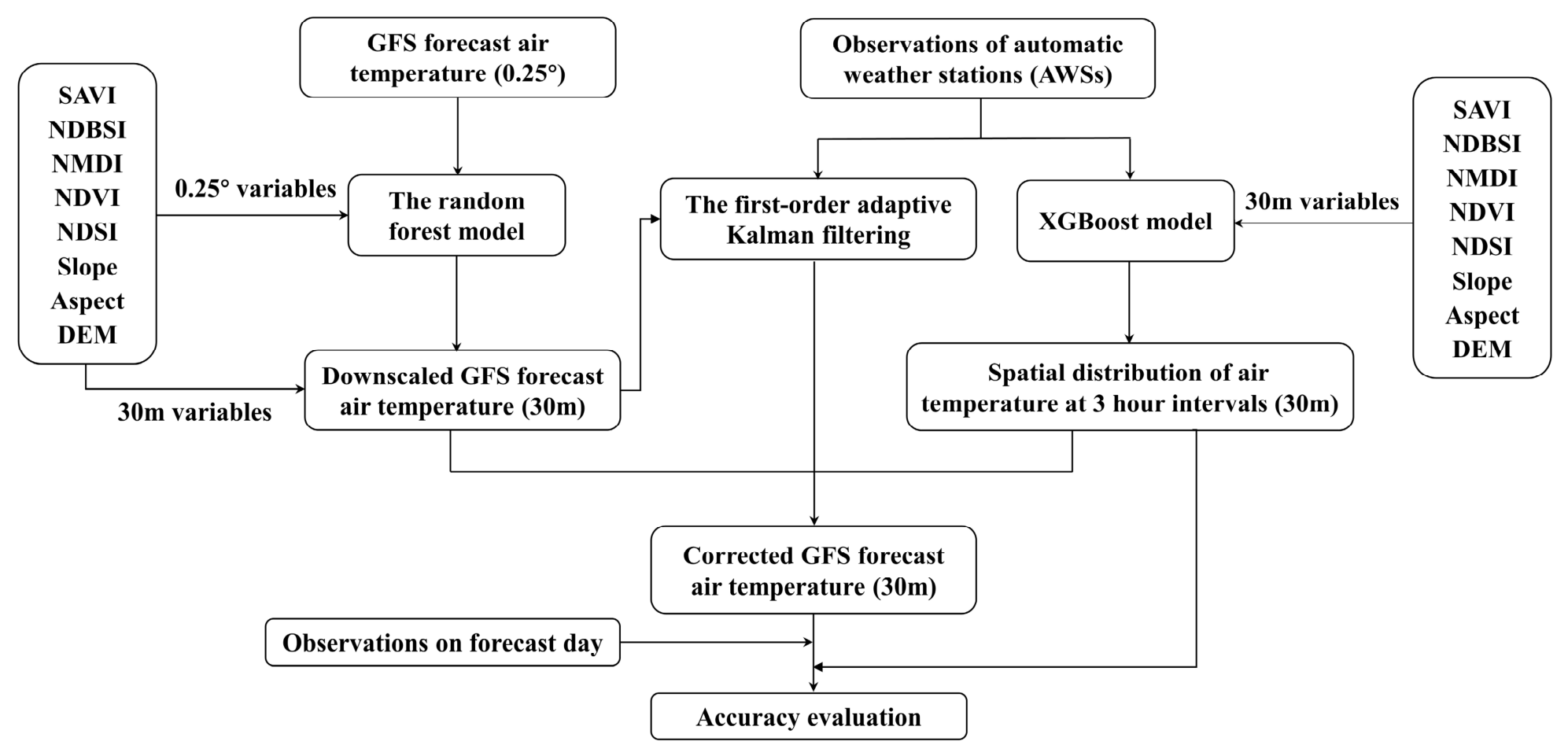
A two steps scheme named DOWN + BC, which integrates direct downscaling (DOWN) with a bias correction (BC) model, was developed to enhance the spatial resolution and accuracy of raw GFS air temperature forecasts in mountainous areas (Figure 2). This method enables the generation of 3-hourly air temperature forecasts at a 30 m grid spacing for the upcoming 24 h without depending on real-time AWS observations.

Figure 2. Flow chart of this study.

The technical workflow of this study, illustrated in Figure 2, consists of the following steps: (a) downscale the raw GFS temperature forecasts using a random forest model, with the raw forecasts as the dependent variable and remote sensing indices together with terrain parameters as independent variables; (b) train an XGBoost model to derive the spatial distribution of air temperature at 30 m resolution, using AWS temperature observations as the dependent variable and remote sensing indices along with terrain parameters as independent variables; (c) determine the optimal number of days and weighting coefficients for the first-order adaptive Kalman filtering model based on the difference between AWS-observed temperatures and the downscaled GFS forecasts at corresponding locations; (d) apply the first-order adaptive Kalman filter to correct bias errors in the raw GFS temperature forecasts; (e) evaluate the accuracy of the forecasts after the DOWN + BC processing.

2.3.1. Calculation of Remote Sensing Spectral Indices and Topographic Parameters

The spatial distribution of air temperature in complex terrain is primarily influenced by three categories of factors: land-surface conditions (e.g., land cover type and vegetation cover), local topographic features (e.g., elevation, slope, and aspect), and macrogeographic settings (e.g., latitude, longitude, large-scale climate patterns, and mountain range orientation). To quantify the contributions of these factors, slope and aspect, were derived from the DSM data. Furthermore, several remote sensing indices were calculated from Landsat 8 OLI imagery, including the Soil-Adjusted Vegetation Index (SAVI, with L = 0.5), the Normalized Difference Vegetation Index (NDVI), the Normalized Difference Snow Index (NDSI), the Normalized Multiband Drought Index (NMDI), and the Normalized Difference Built-up and Bare Soil Index (NDBSI). The NDBSI was computed as the average of the Index-Based Built-up Index (IBI) and the Bare Soil Index (SI). The selected influencing factors are summarized in Table 1.

2.3.2. Downscaling Using the Random Forest Method

The statistical downscaling of air temperature forecasts is fundamentally based on the assumption that the relationship between predicted temperature and auxiliary variables remains consistent across scales. Due to the highly complex topography of the study area, where terrain factors modulate solar and longwave radiation, thereby influencing thermal processes [30], and in accordance with previous research [31], the random forest (RF) model was adopted for downscaling. RF model can effectively handle outliers, process high-dimensional data, and reduce overfitting.

RF models were trained on forecast temperatures at 0.25° spatial resolution, with NDSI (applied only in January 2020), NDVI, SAVI, NDBSI, NMDI, DSM, slope, and aspect aggregated to 0.25° resolution as auxiliary variables. Subsequently, these auxiliary variables computed at 30 m resolution were input to the trained model to generate downscaled temperature forecasts. Since the performance of machine learning models is highly sensitive to hyperparameter settings, a grid-search approach with 5-fold cross-validation was applied to identify the optimal RF parameters. Based on GFS data from January 2020 and July 2023, the selected optimal parameters are n_estimators = [600, 800]; min_samples_split = [36, 18]; min_samples_leaf = [24, 4]; max_features = [‘log2’, ‘log2’]; max_depth = [14, 12]; bootstrap = [‘T’, ‘T’]. The corresponding main equations are as follows:

$$T_c^{\prime }=f({\mathrm{var}}_c)$$

(1)

$${\Delta }_c=T_c-T_c^{\prime }$$

(2)

$$T_f^{\prime }=f({\mathrm{var}}_f)+{\Delta }_f$$

(3)

where $f$ is the trained RF model between the air temperature forecasts and the auxiliary variables at a coarse grid spacing, $T_c$ is the raw GFS air temperature forecast, $T_c^{\prime }$ is the RF model-derived temperature at a coarse grid spacing, $T_f^{\prime }$ is the RF model-derived temperature at a fine grid spacing, ${\mathrm{var}}_c$ and ${\mathrm{var}}_f$ are the regressors at the coarse and fine grid spacings, respectively, and ${\Delta }_c$ is the residual error of the fit, which was interpolated to obtain ${\Delta }_f$ at 30 m resolution.

2.3.3. Spatial Mapping of the Air Temperature from AWS Observations

Given that the first-order adaptive Kalman filter model relies exclusively on available station measurements to adjust predicted air temperatures and given that only 73 (in January 2020) and 42 (in July 2023) AWS supply such data within the study area, AKF-based corrections cannot be applied to locations without observations. To address this limitation, a spatial interpolation method is required to estimate temperatures across unmonitored areas, since the vast majority of grid points on the 30 m resolution grid do not coincide with AWS locations. To date, various methods have been used to produce spatially continuous air temperature data [32,33]. After evaluating the performance of five machine learning approaches including K nearest neighbors, support vector machine, random forest (RF), adaptive boosting, and XGBoost, the XGBoost model was selected to generate a continuous observed-temperature field by spatially extrapolating measurements from available AWS to all grid points. This gridded observed-temperature dataset was subsequently used to perform bias correction on the RF downscaled forecasts and to validate the bias corrected temperatures at a 30 m grid spacing. The choice of XGBoost was based on its superior accuracy, scalability, and predictive capability, as well as its established application in meteorological research [34,35].

Observed temperature data from 52 and 30 AWSs (approximately 70%), along with NDVI, NDSI (January 2020 only), SAVI, NDBSI, NMDI, DSM, slope, and aspect data, were used to train the XGB-derived models for January 2020 and July 2023, respectively. The data from the remaining 21 and 12 stations (approximately 30%) were employed for validation.

2.3.4. Bias Correction Using First-Order Adaptive Kalman Filtering

The first-order adaptive Kalman filtering method was employed to correct forecast outputs by estimating systematic errors. Through weighted averaging, it enhances state estimation accuracy, producing estimates that are closer to the true values [22]. The algorithm is computationally efficient, requiring fewer computational resources and a smaller historical sample size. Additionally, it demonstrates strong adaptability to frequent updates in forecast models and assimilation systems, making it well-suited for practical meteorological applications [36].

In this study, the model error $M(n)$, which is used to correct the forecast day bias, was iteratively calculated using the historical AWS temperature observations and the downscaled temperatures from the random forest model at the corresponding locations. $M(n)$ can be calculated as follows:

$$Y(n)=f(n)-O(n)$$

(4)

$$M(n)=(1-w)M(n-1)+wY(n)$$

(5)

where $Y(n)$ is the forecast error, $f(n)$ is the downscaled predicted temperature, $O(n)$ refers to the observed temperature at AWS locations and the XGBoost model-estimated value for non-AWS measurement locations, n denotes the data of the corresponding time on n days before the forecast day, $M(n)$ is the model forecast error at the corresponding time, and w denotes a weighting factor that controls the influence of recent errors $Y(n)$ relative to historical errors $M(n-1)$.

Once the model error $M(n)$ is obtained, the data for forecast day $n+1$ (i.e., tomorrow) can be corrected.

$$T(n+1)=f(n+1)-M(n)$$

(6)

where $T(n+1)$ is the corrected forecasted value for the corresponding time on day $n+1$, obtained by adjusting the forecast using the model error $M(n)$. Moreover, $f(n+1)$ is the downscaled temperature forecast on day $n+1$. To correct the data at a specific time, only historical observation data at AWS locations and forecast data of that specific time are used. For example, the downscaled GFS temperature data and AWS observation data from historical days D7 to D11 (n = 5) at 12 a.m. local solar time are input into Equations (4) and (5) to calculate the historical error $M(n)$, and the results are then substituted into Equation (6) to correct the forecast data of 12 a.m. local solar time on forecast day D12.

2.3.5. Evaluating the Accuracy of the DOWN + BC Forecasts

The AWS observation data and the XGB-derived air temperature distribution were used as the reference to evaluate the accuracy of the DOWN + BC forecasts. The root mean square error (RMSE), mean absolute error (MAE), and coefficient of determination (R²) are adopted as the accuracy evaluation metrics. RMSE measures the standard deviation of the residuals and is sensitive to outliers; MAE represents the average magnitude of errors without considering their direction; and R² indicates the proportion of the variance in the dependent variable that is explained by the model. These three metrics enable a systematic and comprehensive assessment of the errors in downscaling and correction results.

3. Results and Analyses

3.1. AWS Observation Verification of the DOWN + BC Air Temperature Forecasts

On the basis of the AWS-observed air temperature data, the accuracy of the DOWN step was generally greater than that of the raw GFS forecasts. Compared with those of the raw GFS forecasts, the DOWN result exhibited an increase in R² of 0.06 and a reduction in the average RMSE of 3.24%. However, in numerical terms, the downscaled result did not exhibit a significantly greater improvement than the raw GFS temperature forecasts did. A further correction is thus warranted.

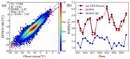
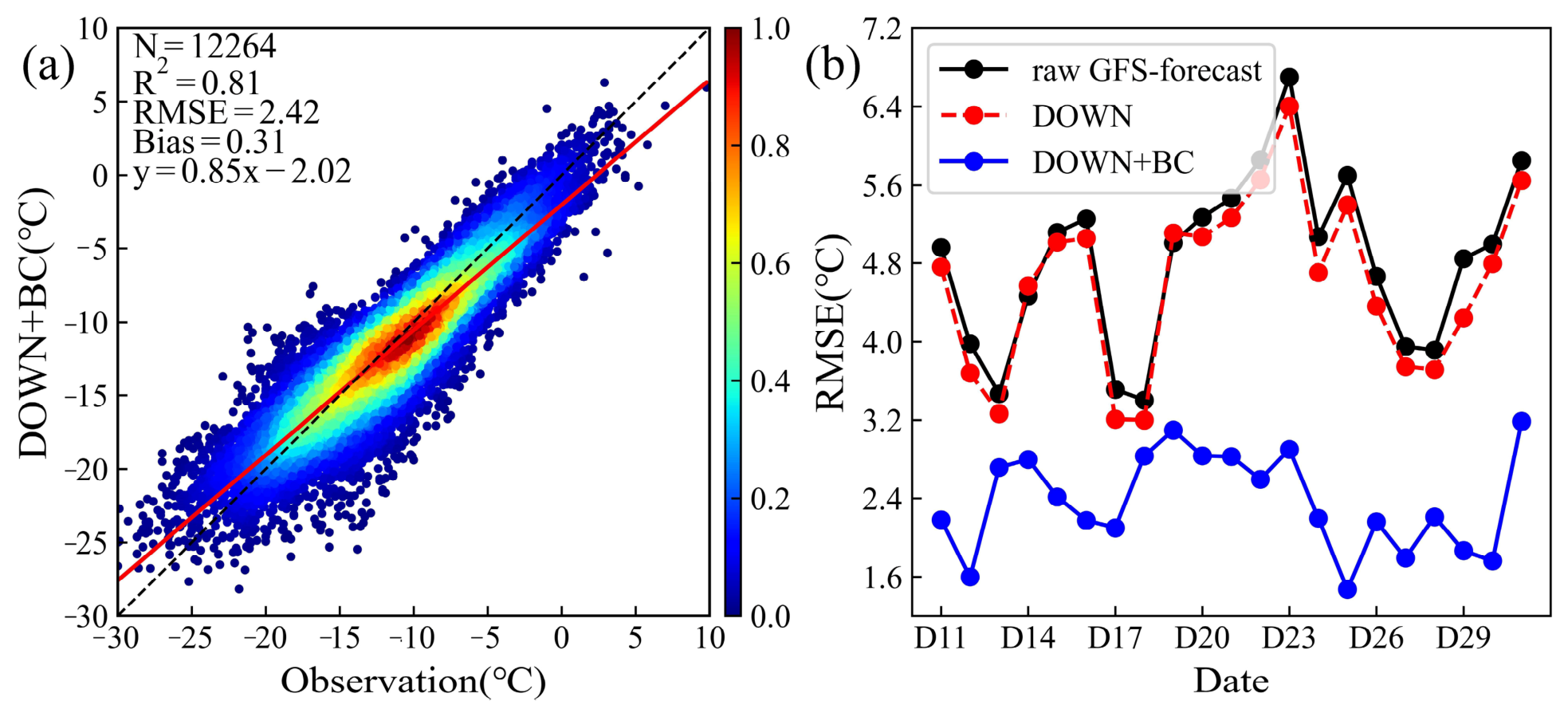
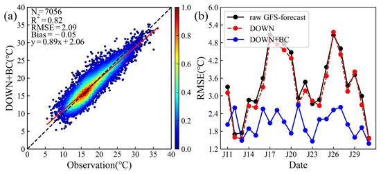
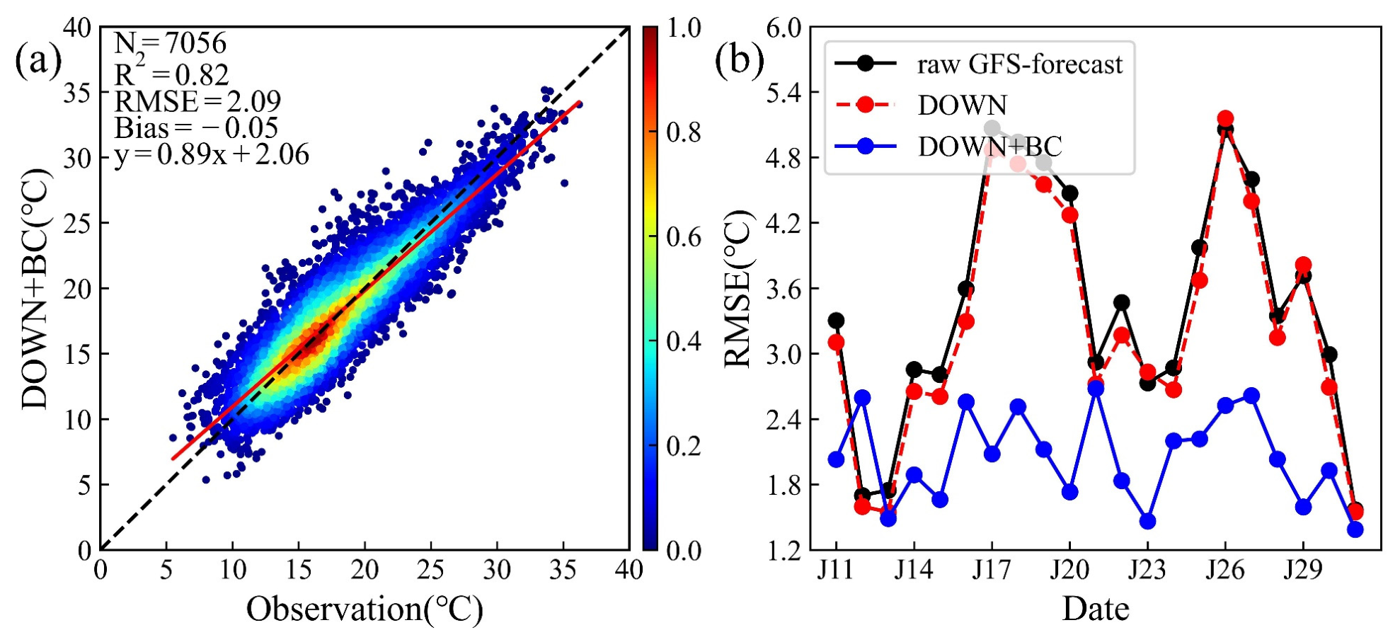
Figure 3a and Figure 4a show that the RMSE values of the DOWN + BC model for GFS-forecast periods D11–D31 and J11–J31 are 2.42 °C and 2.09 °C, respectively. Compared with those of the raw GFS-forecast data at the AWS locations, the RMSE values were reduced by 37.84% and 41.16%, respectively. This finding indicates that the DOWN + BC model performs well in both higher- and lower-temperature ranges. As shown in Figure 3b and Figure 4b, the downscaled air temperatures corrected by the DOWN + BC model are more accurate than the raw GFS model forecasts and the DOWN result. This finding indicates that the DOWN + BC model maintains high prediction accuracy even as the sample size increases significantly. This further demonstrates the stability of the DOWN + BC model across different periods and air temperature ranges.

Figure 3. Scatter plot between the DOWN + BC forecasts and the AWS observations (a), and the daily average RMSE values of the raw GFS forecasts, DOWN, and DOWN + BC results (b) for D11–D31, January 2020.

Figure 4. Scatter plot between the DOWN + BC forecasts and the AWS observations (a), and the daily average RMSE values of the raw GFS forecasts, DOWN, and DOWN + BC results (b) for J11–J31, July 2023.

However, as shown in Figure 3a and Figure 4a, the linear fit in the scatter plots indicates a conditional bias in the DOWN + BC model. There was also a significant difference in the intercepts between the two temperature ranges. Under lower-temperature conditions, the intercepts of the GFS data are −2.02 °C, whereas under higher-temperature conditions, the intercept of the GFS data is +2.06 °C. This suggests that the distribution of the DOWN + BC model forecast air temperatures across the different periods and station locations is narrower than that of the observed temperatures. Specifically, the model forecasts do not capture the full range of the observed extreme air temperatures. Despite this conditional bias, the overall accuracy remains high, as reflected by the R² and RMSE values. These results indicate that the accuracy of the DOWN + BC model can still be enhanced by reducing conditional biases, particularly under lower-temperature conditions.

The hourly RMSE values of the DOWN + BC model compared with those of the raw GFS forecasts (42 cases × 8 h per case) are shown in Figure 5. A total of 91.07% of the time, or 306 times, the DOWN + BC model exhibited a lower RMSE than the raw GFS forecasts. This demonstrates that the proposed DOWN + BC model can effectively downscale and correct the GFS model-predicted air temperature.

Figure 5. RMSE values of the DOWN + BC model compared with those of the raw GFS forecasts at the AWS locations ((a): three-hourly raw GFS forecasts and DOWN + BC (D11–D31); (b): three-hourly raw GFS forecasts and DOWN + BC (J11–J31)).

3.2. Gridded Verification of the DOWN + BC Forecasts

3.2.1. The Accuracy of the Air Temperature Distribution Estimated by the XGBoost Model

The air temperature estimated by the XGBoost model was first validated against AWS observations and then used to evaluate the accuracy of the DOWN + BC forecasts. The optimal hyperparameters were filtered using the same approach as described for the RF model in Section 2.3.2. The optimal model parameters for January 2020 and July 2023 are as follows: n_estimators = [700, 600]; reg_lambda = [0.2, 0.6]; reg_alpha = [0.4, 0.5]; subsample = [0.6, 0.8]; max_depth = [29, 36]; learning_rate = [0.2, 0.4]; gamma = [0.3, 0.2]; colsample_bytree = [0.4, 0.5].

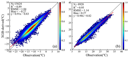
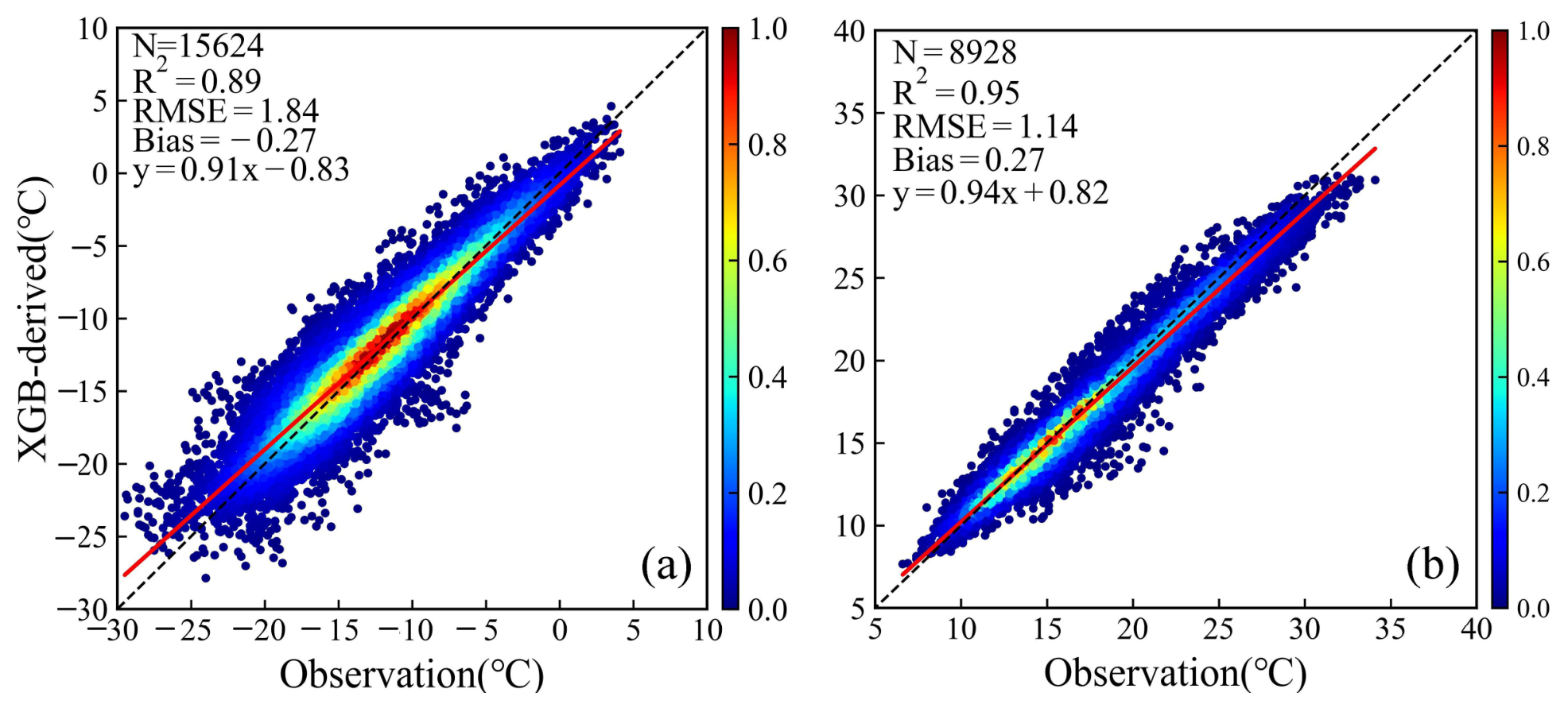
The left and right panels of Figure 6 show scatter plots of the AWS-observed air temperatures against the XGB-derived values at the AWS locations during days D1–D31, 2020 and J1–J31, 2023. The results indicated that the XGB-derived estimates could effectively capture the spatial distribution of the observed temperatures with a relatively high accuracy (the R² and RMSE values for the D1–D31 and J1–J31 periods were 0.89, 1.84 °C and 0.95, 1.14 °C, respectively).

Figure 6. Scatter plots between the observed and XGB-derived air temperatures at the validation sites for the D1–D31 period on January 2020 (a) and the J1–J31 period on July 2023 (b).

From D1 to D31 of 2020, the performance of the XGB-derived model was notably influenced by the frequent wintertime nighttime temperature inversions in mountainous areas. Of the 21 validation stations used in winter, 14 are located at elevations exceeding 1500 m. To further evaluate the model’s accuracy, the data were separated into two intervals: daytime (06:00–21:00) and nighttime (22:00–05:00). The RMSE during the daytime period was 1.56 °C, while it rose to 2.31 °C at night. The latter period aligns with the peak occurrence of temperature inversions in winter mountains, where their varying intensity and shifting spatial distribution contributed to the decline in model performance. Temperature inversion continues to pose a key challenge for predicting winter nighttime temperatures in mountainous regions.

In the winter experiment (D1–D31), on the basis of the XGB-derived model, the importance of each parameter was ranked as DSM > slope > aspect > NDSI > NDBSI > NDVI > NMDI > SAVI, whereas in the summer experiment (J1–J31), the ranking was DSM > NDVI > slope > aspect > NMDI > NDBSI > SAVI. The DSM data exhibited the highest importance during both seasons, with values of 39.44% in winter and 33.16% in summer. Slope and aspect also attained relatively high importance levels, highlighting the strong correlation between the topography and mountain air temperature. Furthermore, the importance of the NDVI, NMDI, NDBSI, and SAVI increased in summer compared with that in winter, with that of the NDVI increasing from 6.54% to 14.64%, for example. This suggests that vegetation plays a role in controlling temperature variations in mountainous areas, but its influence is primarily observed when photosynthetically active vegetation is present.

3.2.2. The Influence of Key Parameters on the Performance of the AKF Model

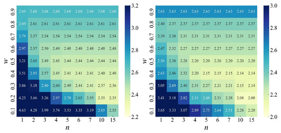
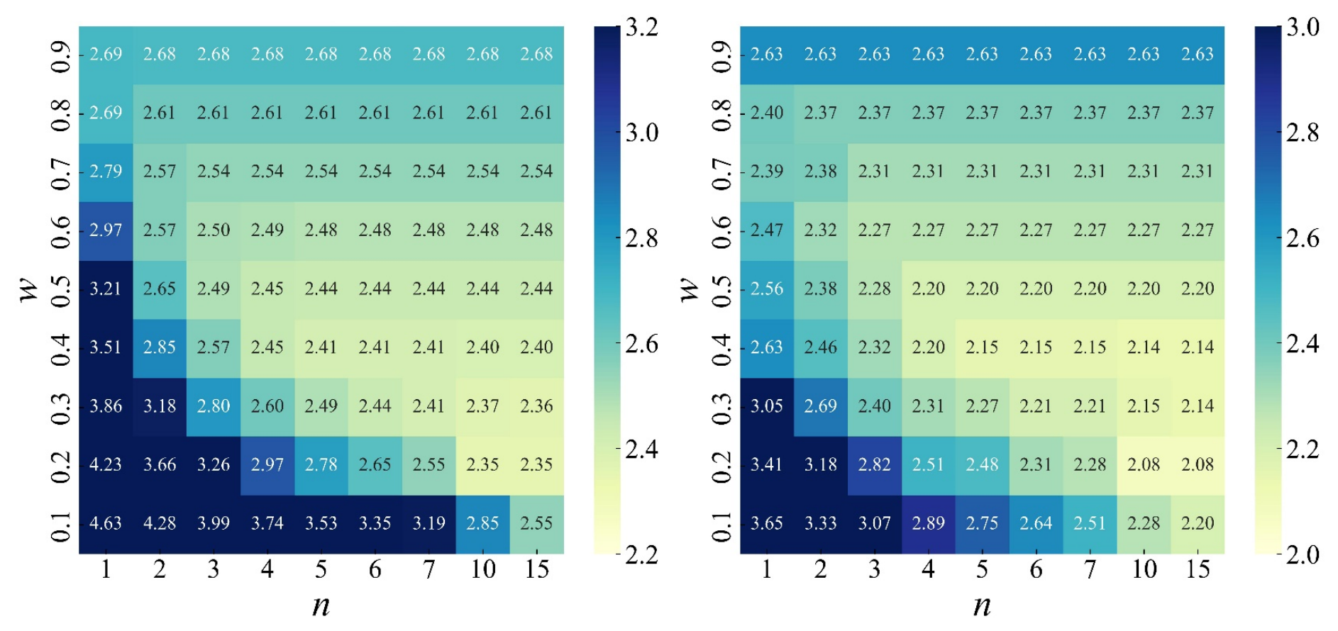
As indicated in Equations (4)–(6), the two key parameters governing the performance of the first-order adaptive Kalman filter model are the length of the historical data period (n) and the weighting factor (w). Over the study area, the diurnal temperature range can exceed 15 °C in both winter and summer. Applying the AKF model directly to correct hourly temperatures may thus result in two distinct extremes: using a larger w improves daytime temperature corrections, whereas a smaller w yields greater accuracy for nighttime temperatures. Extending the historical data period (n) can help reduce AKF errors arising from sharp day-to-day temperature changes. However, since the model error is continuously updated on the basis of historical data, the influence of the initial historical data on the AKF correction accuracy gradually decreases over time. Thus, merely increasing n does not guarantee improved forecast precision. A sensitivity analysis was therefore performed to identify the optimal combination of n and w.

Figure 7 shows the RMSE values for the GFS forecasts corrected using the DOWN + BC method for D16–D31, 2020 and J16–J31, 2023 under different numbers of historical days (n) and weight factor w. Notably, the forecast accuracy increased slightly with increasing number of historical days. However, the improvement gradually plateaued, with minimal gains beyond 5 to 10 days. Based on Figure 7, the optimal weighting parameters are set w = 0.2 and n = 10, and the RMSE values for the best parameters for these two months were 2.35 °C and 2.08 °C.

Figure 7. Comparison of the RMSE (°C) values of the DOWN + BC derived GFS forecasts for different $\mathrm{n}$ and $\mathrm{w}$ values ((left): RMSE of D16–D31, 2020; (right): RMSE of J16–J31, 2023).

3.2.3. Verification of DOWN + BC Forecasts Against Gridded Air Temperature Data

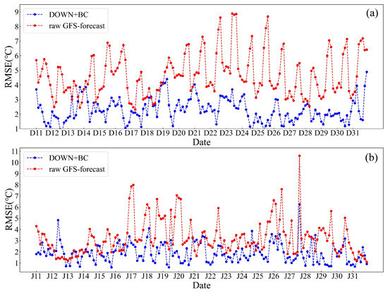
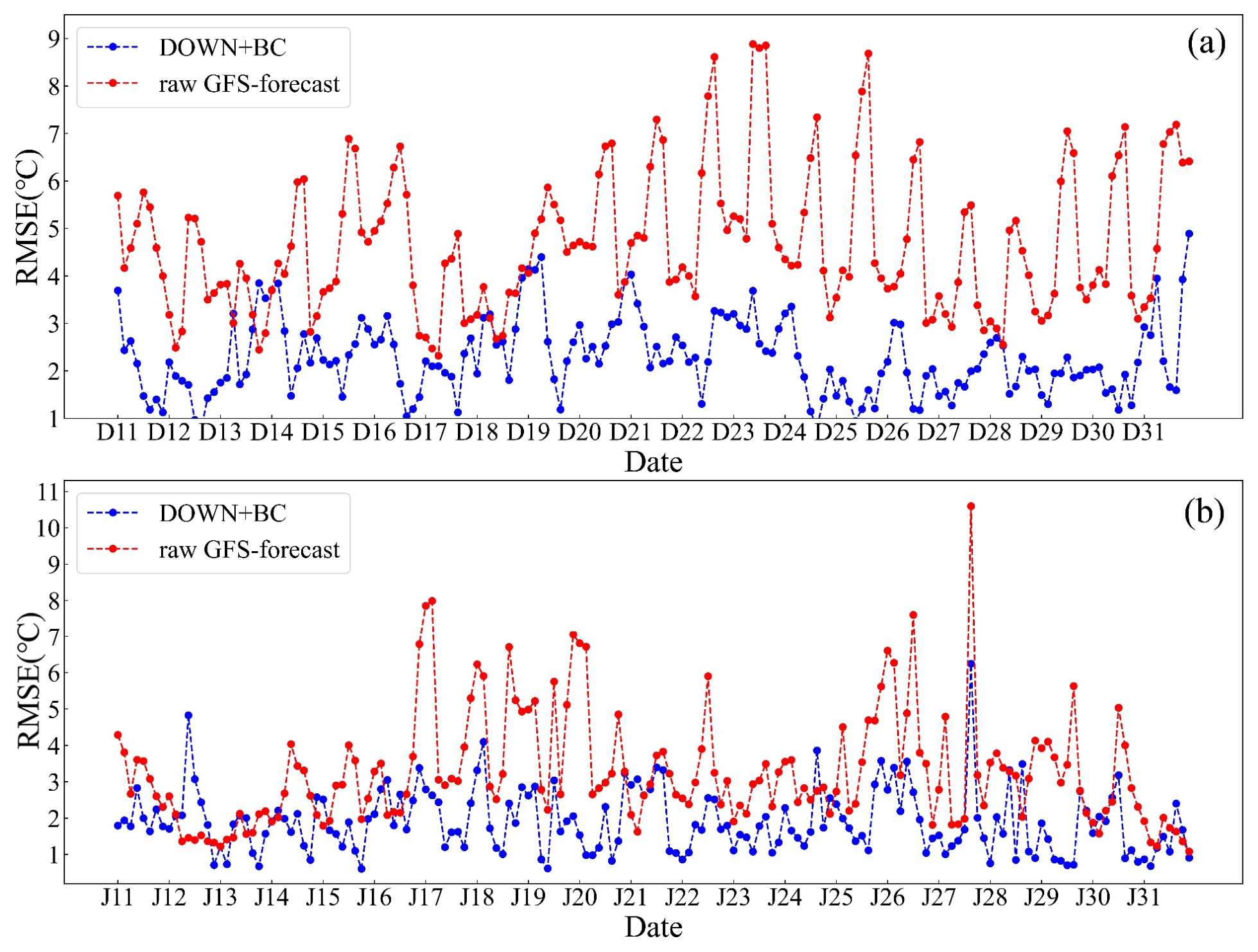
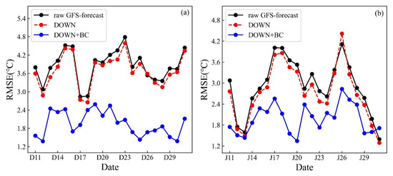
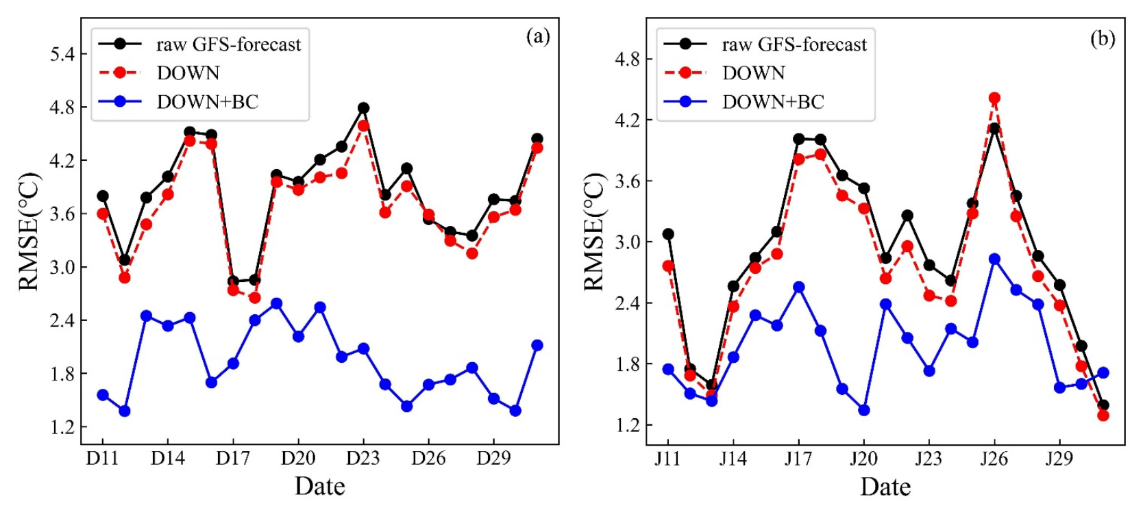
While deviations may exist between the XGB-derived and true spatial air temperature distributions, the accuracy analysis in Figure 6 indicates that the XGB-derived spatial distribution can approximate that of the observed air temperatures. Via the use of the XGB-derived air temperature as a proxy for the observation temperatures at the 30 m grid scale as the validation data, the RMSE values of the raw GSF-forecasts and DOWN + BC model for the forecast days can be calculated, as shown in Figure 8. The RMSE values of the DOWN + BC model were smaller than those of both the raw GFS forecasts, with RMSE reductions of 47.27% and 33.79%, respectively.

Figure 8. Daily average RMSE values on the forecast day for the raw GFS forecasts and the DOWN + BC model validated by the XGB-derived air temperature data ((a): D11–D31; (b): J11–J31).

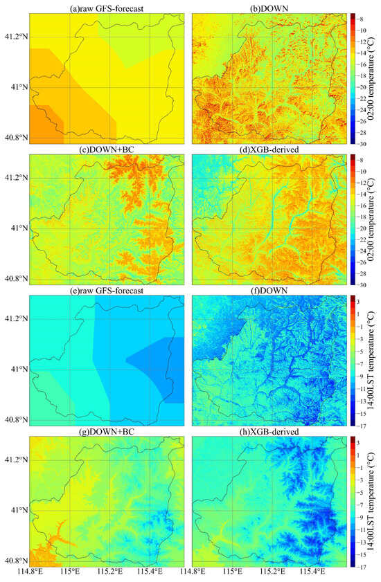
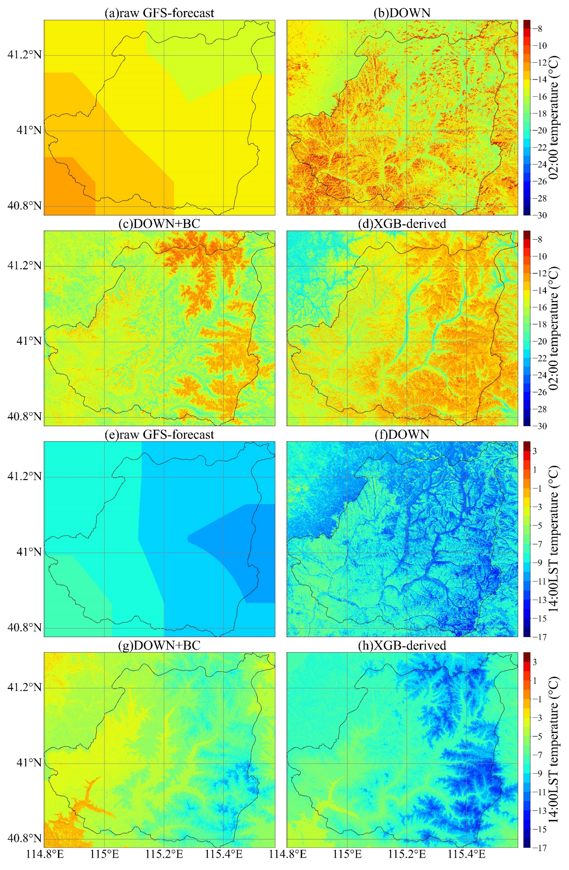
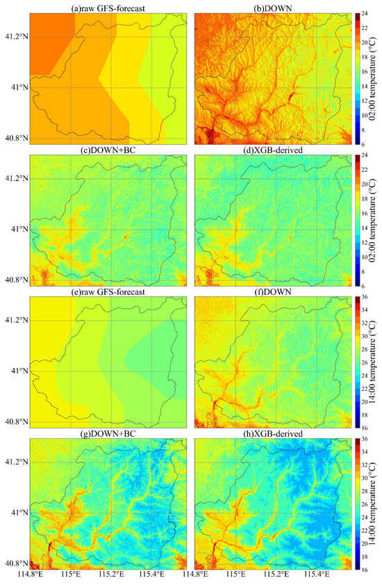
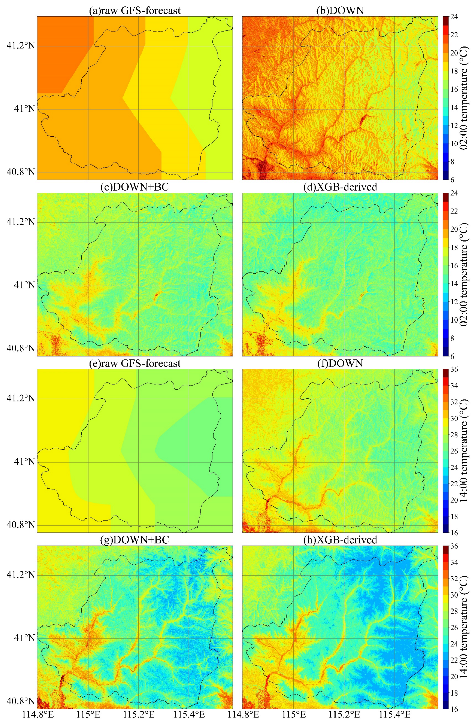
In terms of the spatial distribution, Figure 9 and Figure 10 show the raw GFS forecasts, DOWN, DOWN + BC and XGB-derived air temperatures, respectively, at 2:00 and 14:00 local solar time on D18 and J18.

Figure 9. Spatial distributions of the temperature at 2:00 and 14:00 local solar time on D18 for the raw GFS forecast, DOWN, DOWN + BC, and XGB-derived distribution.

Figure 10. Spatial distributions of the temperature at 2:00 and 14:00 local solar time on J18 for the raw GFS forecast, DOWN, DOWN + BC, and XGB-derived distribution.

As shown in Figure 9g,h and Figure 10g,h, the spatial distribution of the DOWN + BC model closely matches that of the XGB-derived air temperatures. In contrast, as shown in Figure 9a–d and Figure 10a–d, the spatial distributions of the raw GFS temperature forecasts and the DOWN results significantly differ from those of the DOWN + BC and XGB-derived model. The raw GFS model forecasts do not capture the detailed spatial temperature differences influenced by topography and other factors. In contrast, the spatial distributions of the DOWN + BC and XGB-derived temperatures are finer, particularly in the northeastern and southeastern mountainous regions with higher altitudes, as well as in the low-elevation urban areas in the southwest. For example, at 2:00 local solar time on D18 (Figure 9d), the temperatures are relatively high in the high-altitude mountainous areas to the northeast and southeast. Conversely, at 14:00 local solar time on D18 (Figure 9h) and J18 (Figure 10h), the temperatures are relatively low in these mountainous areas and relatively high in the urban areas to the southwest. The spatial distributions of the raw GFS model forecasts differ significantly from the actual conditions. Compared with both the raw GFS forecasts and DOWN model, the DOWN + BC model more accurately captures the spatial distribution of the air temperature, indicating that this model performs well and captures the actual spatial patterns of the temperature with greater precision.

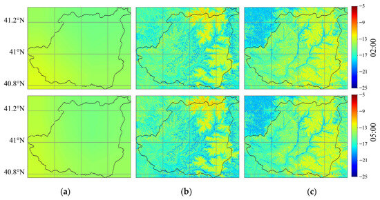
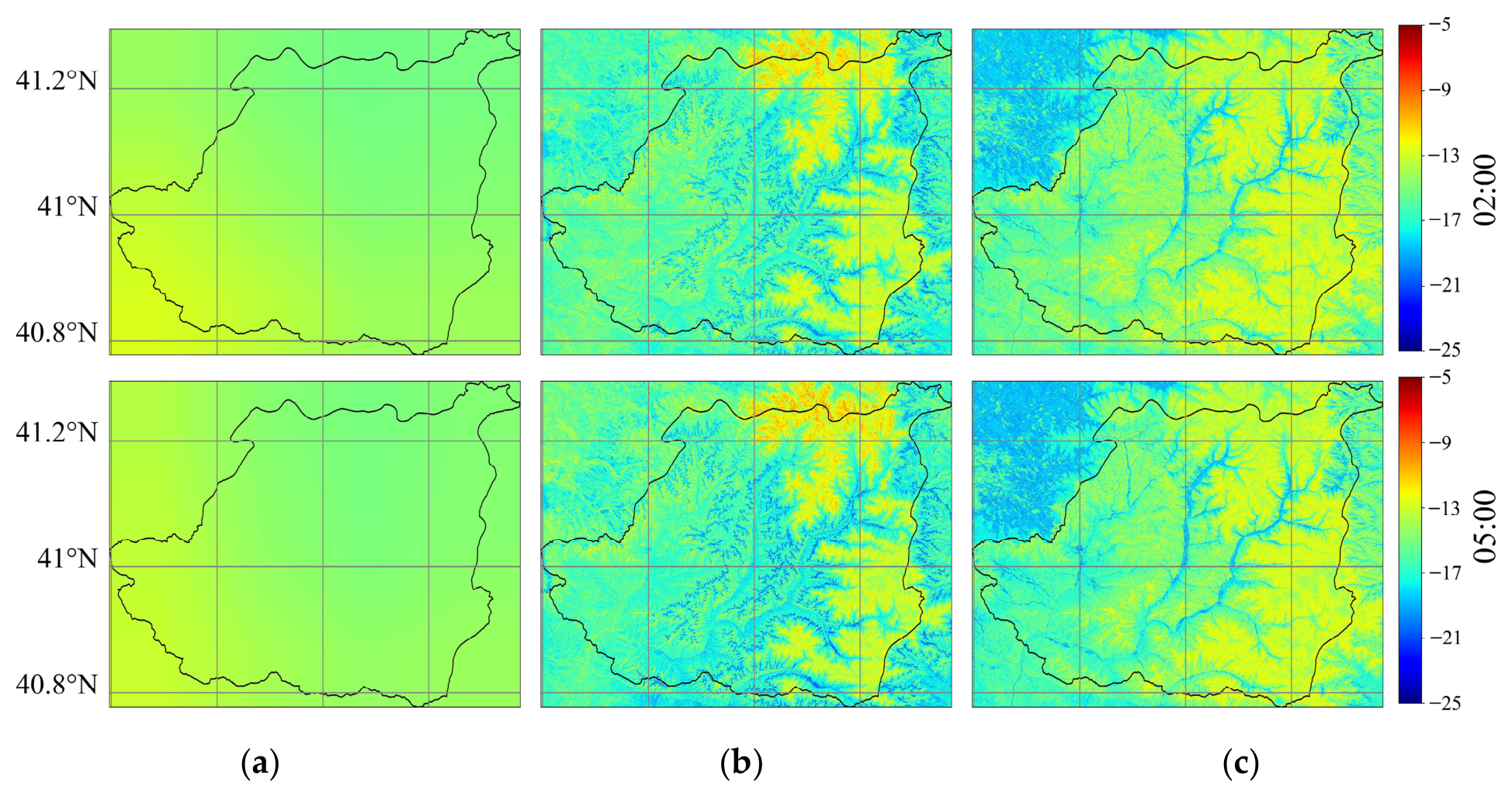
Temperature inversions frequently occur during winter nights, particularly in high-altitude regions (such as the northeastern and southeastern areas). Statistical analysis revealed that during the period from D12 to D29, air temperature inversions were observed 48.61% of the time in the AWS data, with 69.05% of these events occurring between 22:00 and 05:00 local solar time. Adopting the raw GFS forecast at 2:00 and 5:00 local solar time on D18 as the example (Figure 11), the uncorrected raw GFS forecast shows a decrease in the temperature with increasing altitude (Figure 11a) and con not accurately capture the temperature inversion phenomenon, whereas the DOWN + BC forecast and the AWS observational data reveal the opposite trend (Figure 11b,c), with the temperature increasing with increasing altitude. Compared with the raw GFS forecasts, the DOWN + BC model, which incorporates historical data errors, effectively mitigates the impact of temperature inversions, resulting in corrected air temperature forecasts that better agree with altitude variations. These findings further validate the effectiveness of the DOWN + BC method.

Figure 11. Spatial distributions of the air temperature at 2:00 and 5:00 local solar time on D18 for the raw GFS forecast, DOWN + BC, and XGB-derived distribution. (a) Raw GFS forecast; (b) DOWN + BC; (c) XGB-derived distribution.

4. Discussion

Mountain air temperatures are notoriously difficult to forecast accurately due to complex terrain that disrupts standard atmospheric behavior. Steep elevation changes create large vertical temperature gradients, often with inversions and cold-air pooling in valleys. Local circulations like mountain and valley winds further modify air temperatures on small scales. Numerical weather prediction models typically have grid resolutions of several kilometers, which cannot resolve sharp topographic features—an entire mountain slope, peak, and valley may fall into one grid cell, causing significant averaging errors. For example, in a 1 km grid, the difference in altitude between the slope top and foot can reach as much as 500 m, and the temperature difference as high as 3 °C, assuming that the slope of the grid is 0.5 [7]. Sparse observational networks in mountainous regions provide limited data for model initialization and verification. Additionally, uneven cloud cover and precipitation driven by orographic effects produce highly localized temperature variations. All these factors lead to inherently lower forecast accuracy in mountain areas compared to flat terrain.

Aiming to improve air temperature forecasts in mountainous regions, this research proposed the DOWN + BC method to downscale and correct GFS air temperature forecasts. The method was further compared against results from processing WRF forecasts, and its limitations and prospects were also discussed.

4.1. Comparison with the DOWN + BC Results of WRF Forecasts

To evaluate the performance of the DOWN + BC method, which was also applied to downscale and correct air temperature forecasts from the Weather Research and Forecasting (WRF) model, we used the winter season as an example.

The WRF model version 3.7.1, with its center located at 108°E and 38°N, was configured with three domains at 9, 3, and 1 km horizontal grid spacings. Only the outputs from the 1 km domain were used. The model vertical grid spacing was discretized with 50 terrain-following levels, with the model top located at 50 hPa in all the domains. There were 550 grid points along the east–west direction and 484 grid points along the north–south direction in the 1 km domain. Forecast data were collected from 7 January 2020 to 29 January 2020. The NCEP Global Forecast System Final operational global analysis data with a grid spacing of 0.5° were used to determine the initial conditions. Each forecast was initialized at 12:00 local solar time and simulated for the next 36 h. During the initial run of the WRF model, the atmospheric state has not yet been fully adjusted and requires a certain simulation period to reach stability. Therefore, in this study, the first 12 h of simulated data were not used for forecasting, and the actual forecast period extended from 00:00 to 23:00. The various physical parameterization options utilized in this study were as follows: the Thompson parameterization scheme was chosen for microphysics, the Yonsei University parameterization scheme was chosen for the planetary boundary layer, the RRTM longwave scheme and the Dudhia shortwave scheme were employed for radiation, and finally, the Noah land-surface model was adopted as the surface layer scheme.

The DOWN + BC method was then applied to WRF output to obtain hourly air temperature forecasts with a 30 m spatial resolution for the next 24 h. Compared to the WRF forecasts, the RMSE of the DOWN + BC corrected air temperature forecasts decreased by 1.39 °C at AWS locations and by 1.19 °C in spatial distributions, respectively. Compared to the downscaling results of WRF forecasts in January, those of GFS forecasts achieved similar improvements in accuracy at station locations, with increases of 35.55% and 37.84%, respectively. In terms of spatial distribution, the accuracy of GFS-forecast downscaling improved by 47.27%, exceeding the 28.31% improvement achieved by WRF forecast downscaling. The effectiveness of the DOWN + BC method for downscaling air temperature forecasts from WRF and GFS differs due to two main reasons. Firstly, the spatial resolution of WRF forecasts is 1 km, which is higher than GFS’s 0.25°, and the accuracy of WRF forecasts is higher than that of GFS; consequently, GFS forecasts achieve a greater improvement in accuracy after downscaling. Secondly, the use of station-observed air temperatures combined with the Kalman filtering method enables better correction of forecast air temperatures, which is why the accuracy of the DOWN + BC results for both WRF and GFS forecasts is similar at AWS locations.

4.2. Limitations and Prospects

Based on the preceding analysis, the DOWN + BC method demonstrates satisfactory performance with GFS data across both months. Nevertheless, certain limitations and shortcomings remain in the proposed methodology. These issues are detailed below, along with potential directions for future research.

When conducting statistical downscaling from a very coarse resolution (0.25° GFS forecasts) to a high resolution (30 m target), the disparity in spatial scales becomes most pronounced, and the assumption of scale invariance in the downscaling model no longer holds [37]. Moreover, as the spatial resolution span of the downscaling process increases, the accuracy tends to decrease. Therefore, further research is needed to evaluate whether a stepwise downscaling approach incorporating multiple intermediate resolutions can enhance the accuracy of air temperature forecasting across a wide range of spatial scales.

In principle, machine learning downscaling models that account for surface topography and land-surface temperature can provide more detailed and accurate air temperature estimates compared with raw GFS data. In the DOWN experiment, however, no AWS or land-surface temperature data were used, the model relied solely on relationships between temperature forecasts and topographic variables. As a result, it did not yield significant improvements in the forecasted temperatures. The accuracy of the DOWN method mainly depends on the accuracy of the raw GFS forecasts. That said, the method does improve the spatial distribution of the temperature forecasts. Future research could seek to integrate additional variables like wind speed and direction to increase the DOWN model’s accuracy [38]. Moreover, since only statistical downscaling was used here, further work might aim to improve NWP model precision (e.g., via large eddy simulation) or to combine dynamic and statistical downscaling methods.

The bias correction employing first-order adaptive Kalman filtering and the validation of the DOWN + BC model both require data on the spatial distribution of field-measured air temperature. While the XGBoost-derived model provides pixel-level temperature estimates, these are not true measurements and inherently contain errors. Using these estimated temperatures as a reference for evaluating downscaling and correction accuracy may therefore introduce uncertainty. For mountainous areas, encrypting the meteorological stations at reasonable locations is an important and necessary means to obtain more effective air temperature observation data. Vries et al. (2024) designed the AtsMOS workflow to enhance mountain meteorology predictions through the downscaling of coarse numerical weather predictions using local observational data [38]. They concluded that the most significant constraint lies in the AtsMOS workflow’s dependence on the numerical weather prediction data and field data.

Under typical meteorological conditions, the DOWN + BC model substantially reduces forecast errors compared to the raw GFS output. However, its performance degrades under rapidly changing synoptic-scale conditions. This limitation stems from the model error term, M(n), which is derived from long-term historical errors and thus cannot adjust promptly to sharp daily temperature variations. Consequently, the correction factor becomes misaligned with actual conditions, leading to potential overestimation or underestimation in the DOWN + BC-corrected forecasts. For instance, during the experiment, a pronounced temperature inversion in the northern mountainous areas at 02:00 LST on days D16 and D17, followed by a marked cooling on D18, resulted in a warm bias in the corrected temperatures for D18. Downscaling WRF simulations over complex topography also proved that temperature inversions in winter were difficult to forecast accurately [7]. Future work should incorporate hourly, short-term error analysis into the DOWN + BC framework to improve its responsiveness to sudden temperature changes.

5. Conclusions

This study proposes the DOWN + BC method, a two-stage processing framework to generate 3-hourly near-surface air temperature forecasts at a 30 m resolution without real-time AWS data. The method first employs random forest-based statistical downscaling to refine the grid spacing from GFS forecasts, followed by a first-order adaptive Kalman filter for bias correction. Compared to raw GFS outputs, the DOWN + BC model significantly enhances both the spatial detail and the accuracy of the forecasted temperature distribution.

The DOWN + BC model achieved RMSE reductions of 37.84% (D11–D31, 2020) and 41.16% (J11–J31, 2023) compared to raw GFS forecasts at AWS locations. When validated against XGBoost-derived proxy observations at the 30 m scale, RMSE reductions were 47.27% and 33.79% for the respective periods. The DOWN + BC forecasts also showed greater spatial alignment with observations. This indicates the method’s consistent effectiveness in correcting numerical forecasts across different periods and temperature ranges.

To evaluate the accuracy of the downscaled air temperature forecasts, the 3 hourly GFS 0.25° archive dataset in the winter and summer seasons were used to test the DOWN + BC method. This method can also be applied to the latest GFS operational forecasts, which provide temperature data at 1 h resolution for the first 120 h and 3 h resolution from days 5 to 16. Furthermore, the DOWN + BC method holds practical potential for enhancing the spatial resolution of temperature distributions from other numerical weather prediction models.

References

- Gao, L.; Bernhardt, M.; Schulz, K. Elevation correction of ERA-Interim temperature data in complex terrain. Hydrol. Earth Syst. Sci. 2012, 16, 4661–4673. [Google Scholar] [CrossRef] [Scilit]
- Suggitt, A.J.; Wilson, R.J.; Isaac, N.J.B.; Beale, C.M.; Auffret, A.G.; August, T.; Bennie, J.J.; Crick, H.Q.P.; Duffield, S.; Fox, R.; et al. Extinction risk from climate change is reduced by microclimatic buffering. Nat. Clim. Change 2018, 8, 713–717. [Google Scholar] [CrossRef] [Scilit]
- Chung, U.; Seo, H.; Hwang, K.; Hwang, B.; Choi, J.; Lee, J.; Yun, J. Minimum temperature mapping over complex terrain by estimating cold air accumulation potential. Agr. For. Meteorol. 2006, 137, 15–24. [Google Scholar] [CrossRef] [Scilit]
- Mutiibwa, D.; Strachan, S.; Albright, T. Land surface temperature and surface air temperature in complex terrain. IEEE J.-Stars 2015, 8, 4762–4774. [Google Scholar] [CrossRef] [Scilit]
- Lenoir, J.; Graae, B.J.; Aarrestad, P.A.; Alsos, I.G.; Armbruster, W.S.; Austrheim, G.; Bergendorff, C.; Birks, H.J.B.; Bråthen, K.A.; Brunet, J.; et al. Local temperatures inferred from plant communities suggest strong spatial buffering of climate warming across Northern Europe. Glob. Change Biol. 2013, 19, 1470–1481. [Google Scholar] [CrossRef] [Scilit]
- Lembrechts, J.J.; Nijs, I.; Lenoir, J. Incorporating microclimate into species distribution models. Ecography 2019, 42, 1267–1279. [Google Scholar] [CrossRef] [Scilit]
- Zhang, G.; Zhu, S.; Zhang, N.; Zhang, G.; Xu, Y. Downscaling hourly air temperature of WRF simulations over complex topography: A case study of Chongli District in Hebei Province, China. J. Geophys. Res.-Atmos. 2022, 127, e2021JD035542. [Google Scholar] [CrossRef] [Scilit]
- Namdev, P.; Srivastava, P.; Sharan, M.; Mishra, S.K. An update to WRF surface layer parameterization over an Indian region. Dyn. Atmos. Ocean. 2024, 105, 101414. [Google Scholar] [CrossRef] [Scilit]
- Yan, D.; Liu, T.; Dong, W.; Liao, X.; Luo, S.; Wu, K.; Zhu, X.; Zheng, Z.; Wen, X. Integrating remote sensing data with WRF model for improved 2-m temperature and humidity simulations in China. Dyn. Atmos. Ocean. 2020, 89, 101127. [Google Scholar] [CrossRef] [Scilit]
- Hofer, M.; Marzeion, B.; Mölg, T. A statistical downscaling method for daily air temperature in data-sparse, glaciated mountain environments. Geosci. Model Dev. 2015, 8, 579–593. [Google Scholar] [CrossRef] [Scilit]
- Dickinson, R.E.; Errico, R.M.; Giorgi, F.; Bates, G.T. A regional climate model for the western United States. Clim. Change 1989, 15, 383–422. [Google Scholar] [CrossRef] [Scilit]
- Adachi, S.A.; Tomita, H. Methodology of the constraint condition in dynamical downscaling for regional climate evaluation: A review. J. Geophys. Res.-Atmos. 2020, 125, e2019JD032166. [Google Scholar] [CrossRef] [Scilit]
- Zhang, L.; He, C.; Tian, W.; Zhu, Y. Evaluation of precipitation datasets from TRMM satellite and downscaled reanalysis products with bias-correction in Middle Qilian Mountain, China. Chin. Geogr. Sci. 2021, 31, 474–490. [Google Scholar] [CrossRef] [Scilit]
- Pierce, D.W.; Cayan, D.R.; Maurer, E.P.; Abatzoglou, J.T.; Hegewisch, K.C. Improved bias correction techniques for hydrological simulations of climate change. J. Hydrometeorol. 2015, 16, 2421–2442. [Google Scholar] [CrossRef] [Scilit]
- Hu, Y.; Tang, R.; Jiang, X.; Li, Z.-L.; Jiang, Y.; Liu, M.; Gao, C.; Zhou, X. A physical method for downscaling land surface temperatures using surface energy balance theory. Remote Sens. Environ. 2023, 286, 113421. [Google Scholar] [CrossRef] [Scilit]
- Wang, X.; Zhong, L.; Ma, Y.M. Estimation of 30 m land surface temperatures over the entire Tibetan Plateau based on Landsat-7 ETM+ data and machine learning methods. Int. J. Digit. Earth 2022, 15, 1038–1055. [Google Scholar] [CrossRef] [Scilit]
- Colaninno, N.; Morello, E. Towards an operational model for estimating day and night instantaneous near-surface air temperature for urban heat island studies: Outline and assessment. Urban Clim. 2022, 46, 101320. [Google Scholar] [CrossRef] [Scilit]
- Zhang, Z.W.; Du, Q.Y. Merging framework for estimating daily surface air temperature by integrating observations from multiple polar-orbiting satellites. Sci. Total Environ. 2022, 812, 152538. [Google Scholar] [CrossRef] [Scilit] [PubMed]
- Ma, X.L.; Xue, J.S.; Lu, W.S. Preliminary study on ensemble transform Kalman filter-based initial perturbation scheme in GRAPES global ensemble prediction. Acta Meteor. Sin. 2008, 66, 526–536. [Google Scholar]
- Horvath, K.; Koracin, D.; Vellore, R.; Jiang, J.; Belu, R. Sub-kilometer dynamical downscaling of near-surface winds in complex terrain using WRF and MM5 mesoscale models. J. Geophys. Res.-Atmos. 2012, 117, D11111. [Google Scholar] [CrossRef] [Scilit]
- Vujec, I.; Plenković, I.O. Kalman filter sensitivity tests for the NWP and analog-based forecasts post-processing. Meteor. Atmos. Phys. 2023, 135, 1. [Google Scholar] [CrossRef] [Scilit]
- Cui, B.; Toth, Z.; Zhu, Y.; Hou, D. Bias correction for global ensemble forecast. Weather Forecast 2022, 27, 396–410. [Google Scholar] [CrossRef] [Scilit]
- Salomonson, V.V.; Appel, I. Estimating fractional snow cover from MODIS using the normalized difference snow index. Remote Sens. Environ. 2004, 89, 351–360. [Google Scholar] [CrossRef] [Scilit]
- Dirksen, M.; Knap, W.H.; Steeneveld, G.-J.; Holtslag, A.A.M.; Tank, A.M.G.K. Downscaling daily air-temperature measurements in the Netherlands. Theor. Appl. Climatol. 2020, 142, 751–767. [Google Scholar] [CrossRef] [Scilit]
- Zhen, Z.; Chen, S.; Qin, W.; Li, J.; Mike, M.; Yang, B. A modified transformed soil adjusted vegetation index for cropland in Jilin Province, China. Acta Geol. Sin. 2019, 93, 173–176. [Google Scholar] [CrossRef] [Scilit]
- Xu, H.Q. A remote sensing urban ecological index and its application. Acta Ecol. Sin. 2013, 33, 7853–7862. [Google Scholar]
- Yang, G.; Pu, R.; Zhao, C.; Huang, W.; Wang, J. Estimation of subpixel land surface temperature using an endmember index based technique: A case examination on ASTER and MODIS temperature products over a heterogeneous area. Remote Sens. Environ. 2011, 115, 1202–1219. [Google Scholar] [CrossRef] [Scilit]
- Minder, J.R.; Mote, P.W.; Lundquist, J.D. Surface temperature lapse rates over complex terrain: Lessons from the Cascade Mountains. J. Geophys. Res.-Atmos. 2010, 115, D14122. [Google Scholar] [CrossRef] [Scilit]
- Mahrt, L. Variation of surface air temperature in complex terrain. J. Appl. Meteorol. Clim. 2006, 45, 1481–1493. [Google Scholar] [CrossRef] [Scilit]
- Hais, M.; Kučera, T. The influence of topography on the forest surface temperature retrieved from Landsat TM, ETM+ and ASTER thermal channels. ISPRS J. Photogramm. 2009, 64, 585–591. [Google Scholar] [CrossRef] [Scilit]
- Casellas, E.; Bech, J.; Veciana, R.; Miró, J.R.; Sairouni, A.; Pineda, N. A meteorological analysis interpolation scheme for high spatial-temporal resolution in complex terrain. Atmos. Res. 2020, 246, 105103. [Google Scholar] [CrossRef] [Scilit]
- Zhu, S.; Liu, Y.; Hua, J.; Zhang, G.; Zhou, Y.; Xiang, J. Monitoring spatio-temporal variance of an extreme heat event using multiple-source remote sensing data. Chin. Geogr. Sci. 2018, 28, 744–757. [Google Scholar] [CrossRef] [Scilit]
- He, T.; Liu, F.; Wang, A.; Fei, Z. Estimating monthly surface air temperature using MODIS LST data and an artificial neural network in the Loess Plateau, China. Chin. Geogr. Sci. 2023, 33, 751–763. [Google Scholar] [CrossRef] [Scilit]
- Qian, Q.F.; Jia, X.J.; Lin, H. Machine learning models for the seasonal forecast of winter surface air temperature in North America. Earth Space Sci. 2020, 7, e2020EA001140. [Google Scholar] [CrossRef] [Scilit]
- Carrión, D.; Arfer, K.B.; Rush, J.; Dorman, M.; Rowland, S.T.; Kioumourtzoglou, M.-A.; Kloog, I.; Just, A.C. A 1-km hourly air-temperature model for 13 Northeastern US states using remotely sensed and ground-based measurements. Environ. Res. 2021, 200, 111477. [Google Scholar] [CrossRef] [Scilit]
- Zhang, Y.T.; Tong, H.; Sun, J. Application of a bias correction method to meteorological forecast for the Pyeongchang winter Olympic games. J. Appl. Meteor. Sci. 2020, 31, 27–41. (In Chinese) [Google Scholar]
- Li, X.; Zhang, G.; Zhu, S.; Xu, Y. Step-by-step downscaling of land surface temperature considering urban spatial morphological parameters. Remote Sens. 2022, 14, 3038. [Google Scholar] [CrossRef] [Scilit]
- Vries, M.; Matthews, T.; Perry, L.; Thapa, N.; Wilby, R. At-scale Model Output Statistics in mountain environments (AtsMOS v1.0). Geosci. Model Dev. 2024, 17, 7629–7643. [Google Scholar] [CrossRef] [Scilit]
Disclaimer/Publisher’s Note: The statements, opinions and data contained in all publications are solely those of the individual author(s) and contributor(s) and not of MDPI and/or the editor(s). MDPI and/or the editor(s) disclaim responsibility for any injury to people or property resulting from any ideas, methods, instructions or products referred to in the content. |
© 2026 by the authors. Licensee MDPI, Basel, Switzerland. This article is an open access article distributed under the terms and conditions of the Creative Commons Attribution (CC BY) license.