Lithospheric Thermal Structure Beneath East Antarctica Derived from Aeromagnetic Anomaly Analysis

Highlights

What are the main findings?

• A model of laterally variable thermal thickness reveals several hot and thin lithospheric blocks within East Antarctica, including Dronning Maud Land, Gamburtsev Subglacial Mountains, Queen Mary Land and Pensacola Mountains.
• The relatively thick lithosphere of East Antarctica represents the preserved cratonic lithosphere, but local-scale thermal anomalies exist in these regions.

What are the implications of the main findings?

• Thermal anomalies found using our new lithospheric thickness model could serve as a comprehensive framework for understanding the thermal evolution and stability of the ice sheet in East Antarctica.
• Craton thinning indicates that a few cratonic roots have been destroyed by tectonic modifications.

Abstract

East Antarctica is composed of a composite Precambrian shield largely covered by a thick ice sheet. Information on the thermal structure of the East Antarctic lithosphere is critical to the understanding of the geological history and ice sheet dynamics of this region. To better describe the lithospheric thermal structure, Curie-point depths are first estimated through the inversion of aeromagnetic anomaly data using the wavenumber-domain centroid method, and the Curie point estimates is further employed to determine a lithospheric thermal thickness model by integrating the 1D steady-state heat conduction equation. Our results show that the variations in both the Curie-point depth and thermal thickness estimates have strong spatial consistency with known major geological provinces, such as ancient cratons and younger orogens. Moreover, our findings show a hot and thin lithosphere in the Gamburtsev Subglacial Mountains and Dronning Maud Land, whereas a cold and thick cratonic lithosphere is found in the Wilkes and Aurora Subglacial Basins and the hinterland of Enderby Land. A few local-scale thermal anomalies are also observed in cratonic areas, indicating that some of these areas have lost their cratonic signature. The new thermal thickness model provides direct constraints that can be used to trace early tectonic–thermal activities in East Antarctica.

1. Introduction

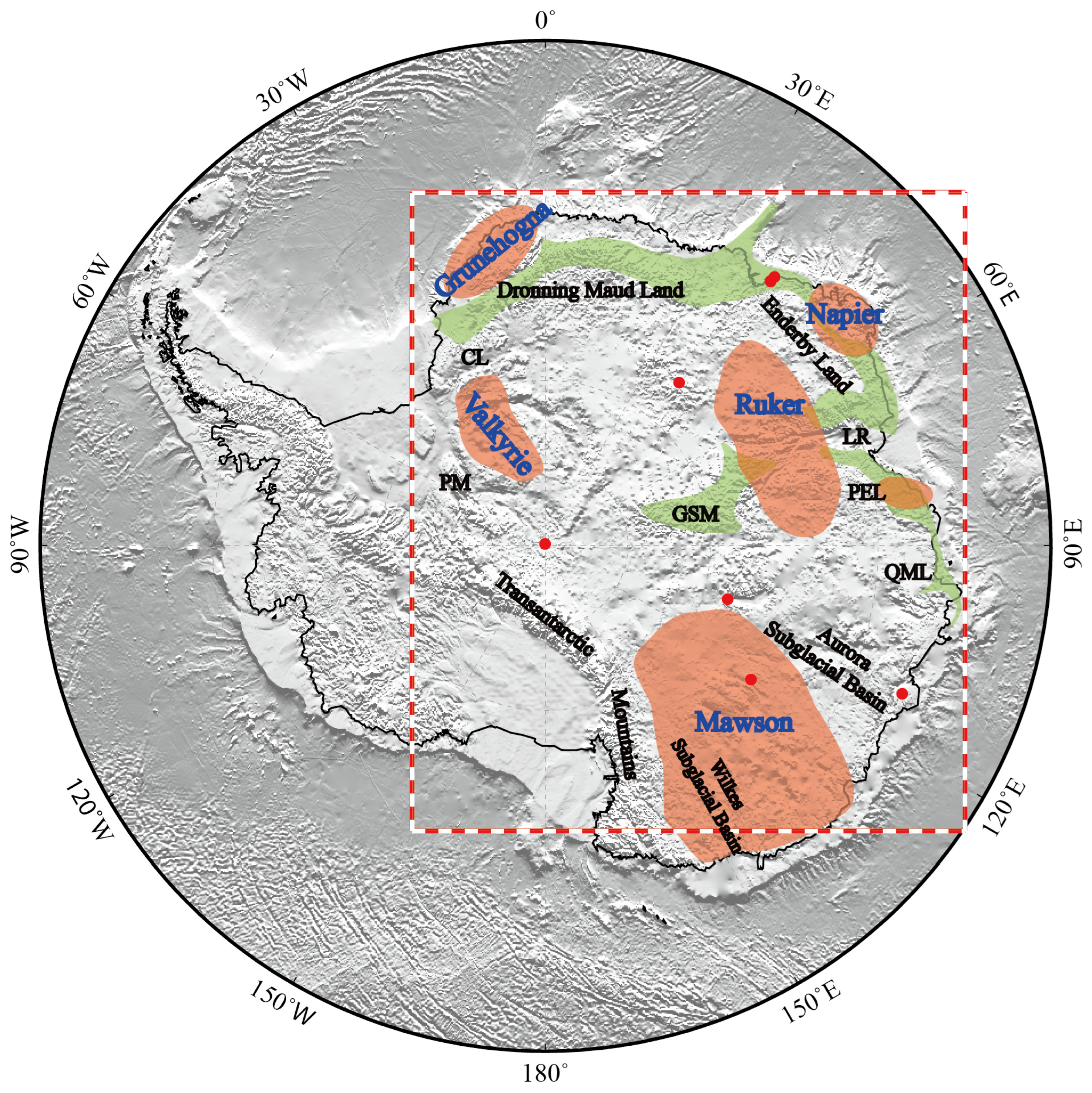
The East Antarctic region (Figure 1) constituted the core of the Gondwana supercontinent, and since the Proterozoic, its lithosphere has undergone multiple phases of tectonothermal activity, characterized by pronounced lithospheric accretion and extension [1]. Throughout the tectonic evolution of East Antarctica, various tectonic units have formed in the lithosphere. These extend from stable Archean cratons through Proterozoic-to-Paleozoic tectonically active intraplate orogens to a Mesozoic rift system [2,3]. Because of its key position, understanding the thermal structure of the East Antarctic lithosphere helps infer crucial geological information about lithospheric deformation and tectonic evolution. However, its thermal state remains poorly constrained due to very limited heat flow measurements (Figure 1). Additionally, East Antarctica is covered by the largest ice sheet on Earth today and hosts a volume of ice equivalent to 52.2 ± 0.7 m of sea-level rise [4]. Ice sheet dynamics and mass balance have important implications for ice sheet behavior and climate change. It is worth noting that geothermal heat beneath East Antarctica is a significant factor affecting ice sheet behavior, acting through heat transfer at the ice–bedrock interface. Therefore, lithospheric thermal thickness and the subglacial thermal state are key factors in revealing the thermal evolution and stability of the ice sheet over East Antarctica.

Directly measuring geothermal heat flow in situ is a very efficient method for obtaining accurate geothermal profiles; however, such surveys are, unfortunately, impossible to complete in high-latitude regions of the Antarctic continent. Because the thick ice sheet cover and harsh weather conditions hinder drilling to the underlying bedrock, it may be extremely difficult to directly measure subglacial heat flow beneath the Antarctic continent. Until now, only a few deep-ice boreholes have been drilled to observe the temperature gradient at the bottom of the ice sheet [5]. Thus, there is major uncertainty regarding the subglacial thermal state of this continent, which makes constructing geological evolutionary models a challenge. To overcome the limitations of subglacial heat flow measurements in East Antarctica, an increasing number of studies have concentrated on indirect observations using other geophysical data, such as seismic, magnetic, gravity and geoid data. An et al. [6] constructed a shear velocity model for the Antarctic plate by inverting tele-seismic surface waves; the model was then converted to temperature model based on the thermoelastic properties of mantle minerals and seismic velocities. Ultimately, they provided a series of lithospheric models, including three-dimensional temperature, Curie-point depth and lithospheric thermal thickness models. Shen et al. [7] employed an empirical correlation between the shear wave velocity of the upper mantle and measured heat flow values in the United States to infer heat flow values across Antarctica. Haeger et al. [8] presented a thermal structure and heat flow model for the Antarctic lithosphere by combining the 1D steady-state heat equation with a converted temperature structure taken from a global seismic velocity model. Wiens et al. [9] extracted variations in the lithospheric thickness of East Antarctica from the seismic velocity model inverted by Lloyd et al. [10], who used an adjoint tomography method to image the velocity structure of the upper mantle and the transition zone beneath the Antarctic continent and its surrounding oceans. Moreover, several lithospheric thickness values near seismic stations deployed on the Antarctic continent are constrained by the seismic S-receiver function [11]. However, they only give robust thickness values in the Transantarctic Mountains and the adjacent West Antarctica region. The hinterland of East Antarctica is unimaged due to the poor quality of seismic data in the region. Compared to seismic data, magnetic data have been increasingly adopted to study thermal structure over Antarctica. Using an equivalent-source magnetic-dipole method, Fox Maule et al. [12] employed satellite magnetic data to infer the thickness of the magnetic crust, and they estimated heat flow values by incorporating the 1D steady-state heat conduction equation into their method. Martos et al. [13] further presented high-resolution Antarctic Curie-point depths and heat flow models using the defractal spectral method based on a new magnetic anomaly model compiled from a satellite-derived magnetic model and available aeromagnetic data. In addition, a few local-scale thermal analyses of Princess Elizabeth Land, the Gamburtsev Subglacial Mountains, and the Wilkes Subglacial Basin were performed with observed magnetic data [14,15,16]. Recently, Pappa et al. [17] used satellite gravity gradient data to estimate the lithospheric thermal structure over Antarctica, and Artemieva [18] also inverted a lithospheric thermal thickness model by jointly modeling gravity and elevation combined with the thermal isostasy method. Afonso [19] demonstrated that geoid height data is more sensitive to deep density anomalies (e.g., lithospheric mantle) than gravity data is; thus, Ji [20] employed geoid, elevation and seismic data to develop a lithospheric thickness model for Antarctica.

Besides these traditional geophysical inversions, a few new methodologies have been developed in recent years that utilize published geophysical models and geological data from other continents to investigate the thermal structure of Antarctica by constructing new heat flow models. For example, Lösing and Ebbing [21] presented a machine learning method to predict heat flow in Antarctica using a series of geological and geophysical datasets. Stål et al. [22] also used abundant geophysical data and models to build an Antarctic heat flow model using the similarity detection approach. Chu et al. [23] proposed a deep learning algorithm and collected global heat flow values and different geological and geophysical features as training data to develop an Antarctic heat flow model. Although several Antarctic heat flow models have been created, the existing continental-scale models show remarkable inconsistencies on a more local scale, including those that focus on the South Pole region, Princess Elizabeth Land, and the Gamburtsev Subglacial Mountains. For example, Martos et al. [13] first provided a continental-scale model of Curie-point depths in Antarctica by combining near-surface and satellite magnetic data. Subsequently, Li et al. [14] employed the newly collected magnetic data to recover Curie-point depths in Princess Elizabeth Land, and they found that noticeable discrepancies exist in this region when compared with Martos’s model, in which satellite data are incorporated and used in the calculations.

Magnetic anomalies reflect the magnetization of rocks in the lithosphere, and measurements show that most ferromagnetic minerals are concentrated in the Earth’s crust [24]. Curie-point depth refers to the isothermal surface (about 550 °C for magnetite) at which ferrimagnetic and ferromagnetic minerals suddenly lose their magnetization [25]. Thus, Curie-point depth measurements could independently reflect the regional thermal structure primarily in the crust. Furthermore, by incorporating the heat conduction equation, the lithospheric thermal structure can be reconstructed, which can provide deeper lithospheric-scale information on the region’s thermal state. Compared to other types of field observations (e.g., geoid and gravity data) that require the conversion of density anomalies into temperature parameters, Curie-point depths derived from magnetic anomaly data could provide a more direct approach to estimating the Earth’s thermal structure. As for seismic studies, apart from the issue of velocity–temperature conversion, the sparse seismic station coverage, especially in East Antarctica, limits the ability to capture data on key tectonic units. Therefore, magnetic data becomes one of the most important foundations in deciphering the deep thermal structure of the East Antarctic lithosphere and studying its geological evolutionary processes.

In this study, we first utilize magnetic anomaly data to invert the Curie-point depths in East Antarctica; we then use the Curie-point estimates as constraints to build geothermal profiles at various positions by solving the 1D steady-state heat conduction equation. Then, we infer high-resolution lithospheric thermal thickness in our study area, constrained by the mantle adiabat. Our results suggest that the Precambrian basement and surrounding orogenic belts are well resolved by the inverted thermal thickness model. Moreover, we compare our results with a previous model of lithospheric thickness, which was derived using independent data [20], to validate our estimation results and examine the origins of large discrepancies. This paper aims to study the large-scale lithospheric thermal structure in East Antarctica, especially in regions where seismic stations and heat flow measurements are sparse, and to understand the tectonic environments and deformation patterns in these areas.

Figure 1. Bedrock topography and bathymetry of Antarctica. The orange and green shading shows the locations of cratons and mobile belts, and the dashed red rectangle denotes the study area [20]. The locations of measured heat flow over East Antarctica are marked by red dots [5]. Key geographic features of East Antarctica are given as follows: CL: Coats Land; GSM, Gamburtsev Subglacial Mountains; LR, Lambert Rift; PEL, Princess Elizabeth Land; PM, Pensacola Mountains; QML, Queen Mary Land.

Figure 1. Bedrock topography and bathymetry of Antarctica. The orange and green shading shows the locations of cratons and mobile belts, and the dashed red rectangle denotes the study area [20]. The locations of measured heat flow over East Antarctica are marked by red dots [5]. Key geographic features of East Antarctica are given as follows: CL: Coats Land; GSM, Gamburtsev Subglacial Mountains; LR, Lambert Rift; PEL, Princess Elizabeth Land; PM, Pensacola Mountains; QML, Queen Mary Land.

2. Data and Methods

2.1. Magnetic Data

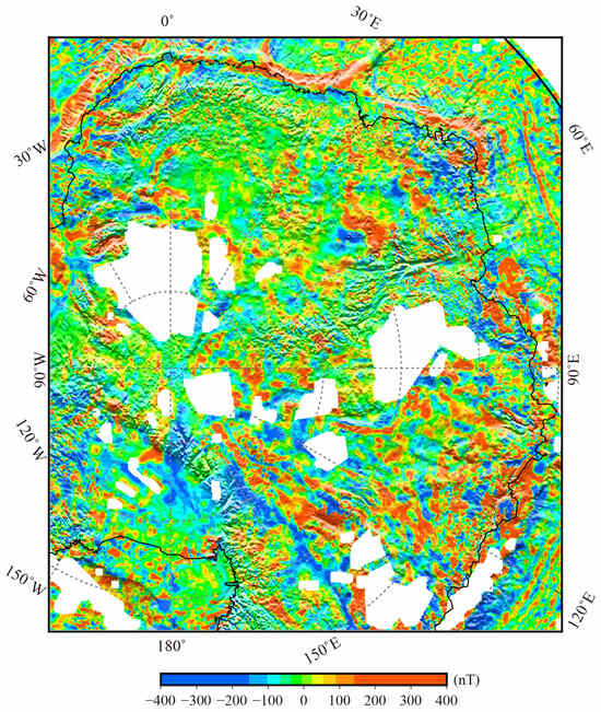
In this paper, we used magnetic data (Figure 2) from the recently released magnetic field model ADMAP-2S [26,27] to calculate the Curie-point depth distribution, which is obtained from a compilation of observations from oceanic, aeromagnetic and satellite data. We removed the satellite magnetic data from the gridded dataset, because recent studies have demonstrated that the process of filling in data gaps caused by the absence of near-surface magnetic anomalies with satellite-derived magnetic data may result in huge errors when estimating Curie-point depth. To ensure the robustness of our models, following Lowe et al. [16], only the measured aeromagnetic data were used to investigate the thermal structure of East Antarctica in this study.

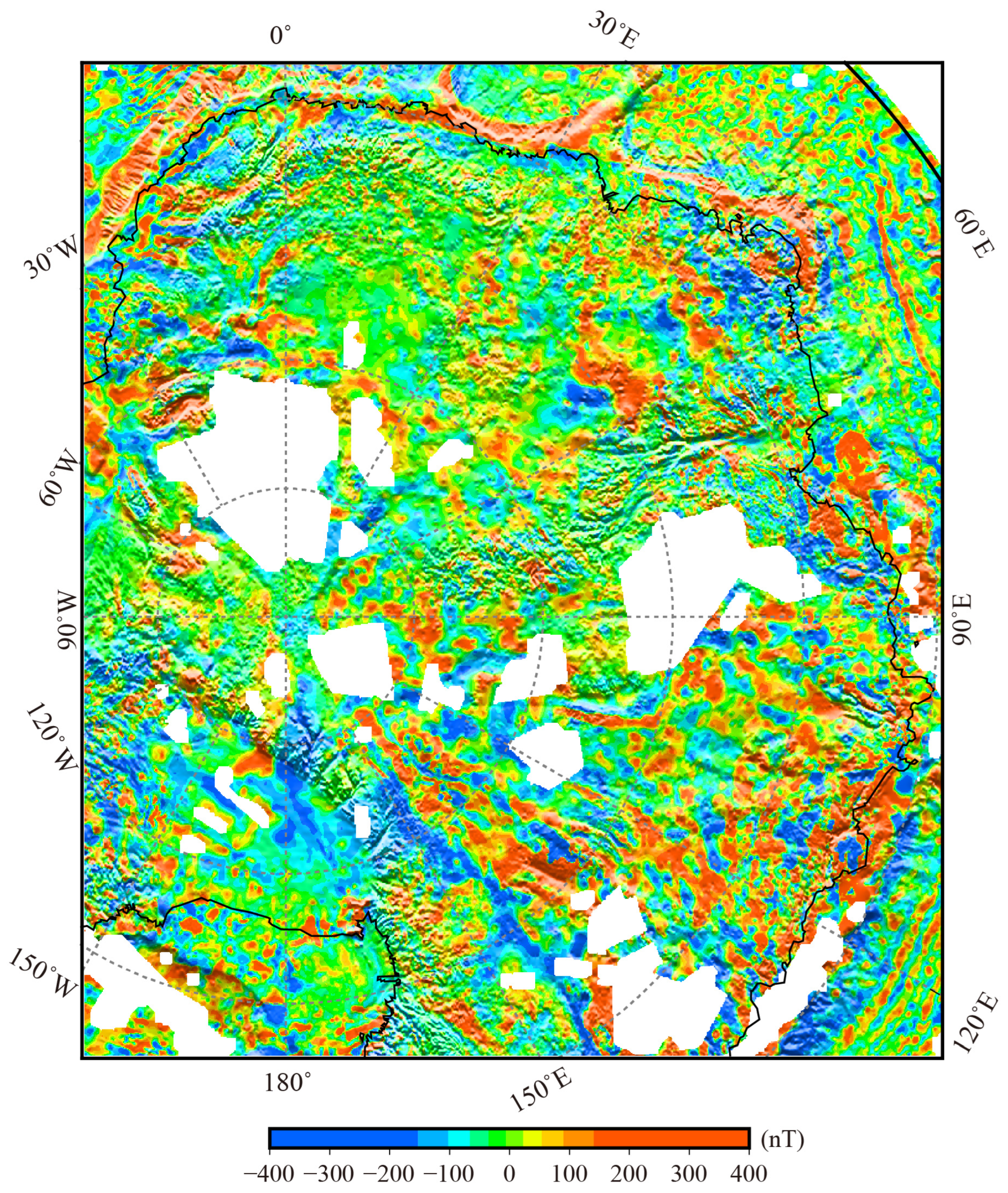
Figure 2. Total magnetic anomaly map of East Antarctica from ADMAP-2S with a grid spacing of 5 km [26,27].

The published magnetic anomaly data are projected in the Polar Stereographic Projection with a latitude of true scale at 71°S, referenced to WGS84 and then interpolated into a 2D rectangular grid with a sampling interval of 5 km. Figure 2 shows that the data coverage density of magnetic surveys varies in different regions. Overall, it is very dense in Dronning Maud Land, Prydz Bay and Victoria Land, while measurements are sparse in some hinterland regions of East Antarctica, including the southern areas of Coats Land, the South Pole region and Princess Elizabeth Land.

2.2. Curie-Point Depth Estimation

In order to calculate Curie-point depth, a modified wavenumber-domain centroid method is employed. This method assumes a fractal magnetization model in which magnetic anomalies are caused by a single magnetized layer confined between bottom and top depths. To date, this method has been successfully applied to various regions and tectonic domains, such as the North Atlantic, western North America, and Northeast China [28,29,30], and these studies show that there are certain advantages in using inverted models to determine the thermal structure. In this fractal magnetization model, the amplitude spectrum of total magnetic anomaly field can be represented as a function of the bottom ($Z_b$) and top ($Z_t$) depths of the magnetic source body [28]:

$$\ln \left[A_{∆T}\left(\left|k\right|\right)\right]=\ln C-\left|k\right|Z_t+\ln \left[1-e^{-\left|k\right|\left(Z_b-Z_t\right)}\right]-{\displaystyle \frac{\beta -1}{2}}\ln \left|k\right|$$

(1)

where $A_{∆T}\left(\left|k\right|\right)$ is the radially averaged amplitude spectrum of the total magnetic anomaly field, C is a constant, $k=\sqrt{{k_x}^2+{k_y}^2}$ is the spatial wavenumber, and $\beta$ is the fractal exponent in the 3D power spectrum, which is unknown before the calculation. As demonstrated earlier, $\beta$ is a significant parameter that has important influence on the estimated $Z_b$ variations [30,31,32]. Commonly, $\beta$ is fixed at a constant value between 1 and 4 according to different tectonic settings. Sobh et al. [32] utilized varying $\beta$ values to estimate the Curie depth in southern Africa, and they showed that larger $\beta$ values can result in shallower $Z_b$ values, and vice versa. Thus, greater $\beta$ values seem to be suitable for regions where $Z_b$ is lower, such as tectonically active zones or areas with a young oceanic lithosphere. To simplify the calculations, a constant value of 1.5 is chosen in this study, which is very similar to that used by Martos et al. [13] for the entire Antarctic continent. Test results using other $\beta$ values are shown in Figure S1 in the Supplementary File. The $Z_b$ value can be estimated using the following three steps.

First, in the medium to high wavenumber domain, Equation (1) can be simplified as

$$\ln \left[{\left(\left|k\right|\right)}^{\left(\beta -1\right)/2}\times A_{∆T}\left(\left|k\right|\right)\right]=\ln B-\left|k\right|Z_t$$

(2)

Second, in the low wavenumber domain, Equation (1) can be rewritten as

$$\ln \left[{\left(\left|k\right|\right)}^{\left(\beta -1\right)/2}\times A_{∆T}\left(\left|k\right|\right)/\left|k\right|\right]=\ln C-\left|k\right|Z_0$$

(3)

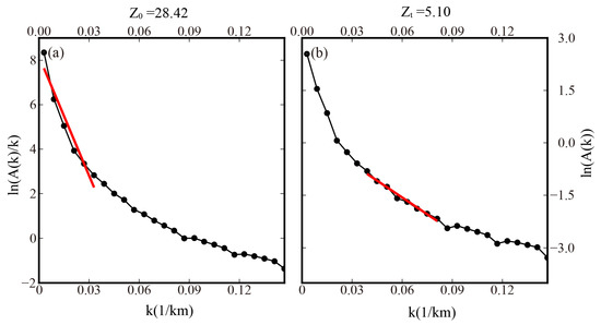
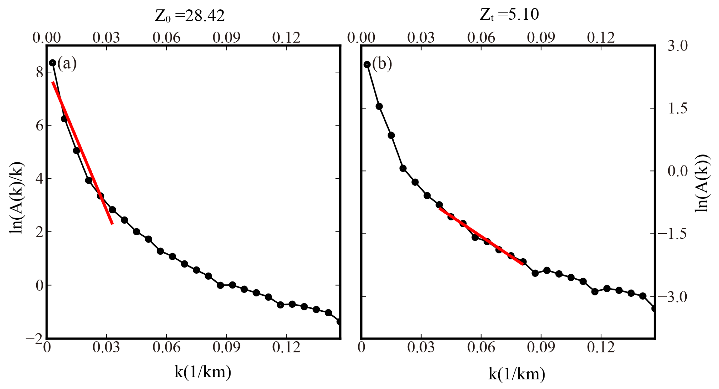
where $Z_0$ is the centroid depth of the magnetic source body. In Equations (2) and (3), $Z_t$ and $Z_0$ can be computed through linear fitting in the radially averaged amplitude spectrum at high and low wavenumbers. An example is given in Figure 3 to show the fitting condition when estimating $Z_0$ and $Z_t$. In the last step, the Curie-point depth $Z_b$ can be calculated via $Z_t$ and $Z_0$ by

$$Z_b=2Z_0-Z_t$$

(4)

Figure 3. An example of the amplitude spectrum from a selected window. (a) Amplitude spectrum to estimate $Z_0$ in the low wavenumber domain. (b) Amplitude spectrum to estimate $Z_t$ in the high wavenumber domain. The red lines indicate the best fit to calculate $Z_0$ and $Z_t$.

In order to develop a spatially variable Curie-point depth map, we divide the entire study region into overlapped 2D finite-size windows. In each window, an optimized value is given, which is found using Equations (2)–(4). During the calculation, after the estimate is made in one window, we move the window center by 50 km; this process continues until estimates have been obtained for all windows.

Following the method described by Okubo and Matsunaga [33], the uncertainty of $Z_t$ and $Z_0$ is calculated based on the deviations ($\sigma$) between the radially averaged spectrum and the linear fit at the specific range of wavenumbers ($∆k$):

$$ϵ={\displaystyle \frac{\sigma }{2\pi ∆k}}$$

(5)

Furthermore, we can obtain the uncertainty of the averaged Curie-point depths (${ϵ}_b$) from that of $Z_t$ and $Z_0$ (${ϵ}_t$, ${ϵ}_0$) using the following equation, in which $N$ = 3 [30]:

$${ϵ}_b={\displaystyle \frac{1}{N}}\sqrt{{\displaystyle \sum _{i=1}^N}\left[{2{{ϵ}_0}^i}^2+{{{ϵ}_t}^i}^2\right]}$$

(6)

2.3. Lithospheric Thermal Model

To study the lithospheric thermal structure, we use the Curie-point depths obtained in the last section as a constraint to develop lithospheric geothermal profiles by solving the 1D steady-state heat conduction equation. This equation is defined as follows, assuming a constant thermal conductivity and an exponentially decreasing distribution with the depth of heat production in the crust [34]:

$$k{\displaystyle \frac{d^{2}T\left(z\right)}{d{z}^2}}+H_0{e}^{-z/h_r}=0,$$

(7)

in which $k$ represents the thermal conductivity, $T\left(z\right)$ refers to the temperature at a depth of z, $H_0$ is the surface heat production, and $h_r$ is the scale depth for the decrease in heat production. The last two parameters are set as 2.5 $\mu \mathrm{W}/{\mathrm{m}}^3$ and 15 km, respectively. Assuming surface temperature $T_0=0 °\mathrm{C}$ and Curie-point temperature $T_c=550 °\mathrm{C}$ as boundary conditions, the geothermal profiles within the magnetic layer can be obtained by solving Equation (7). Laboratory measurements reveal that the thermal conductivity of olivine varies with increasing depth and temperature [35], and this variation can yield inconsistent results. Li et al. [36] mentioned that the maximum temperature difference at a depth of around 75 km is about 6 °C when considering the effect of temperature-dependent thermal conductivity. Following calculations by Wang et al. [29], we could have adopted temperature-dependent conductivity in our model, but this process would introduce new unknown parameters. Therefore, we set the thermal conductivity as 2.5 W/(m⋅°C) in the magnetic layer and 3.0 W/(m⋅°C) below it in this study [20].

To obtain the lithospheric temperature structure beneath $Z_b$, we extrapolate the geothermal profile using a continuous geothermal gradient and a fixed temperature ($T_c$) at a depth of $Z_b$. Once temperature profiles for the entire study region have been constructed, the bottom of the thermal lithosphere can be calculated using the intersection of the estimated geothermal profile and a mantle adiabat, which is expressed as a function of depth ($z$) [34,36]:

$$T_L\approx 1300+0.4z,$$

(8)

where $T_L$ represents the temperature at the bottom of the lithosphere. This study could bridge the knowledge gap between the shallow structure of the magnetic layer and the underlying mantle thermal structure via Curie depths and the heat conduction equation.

3. Results

3.1. Curie-Point Depths

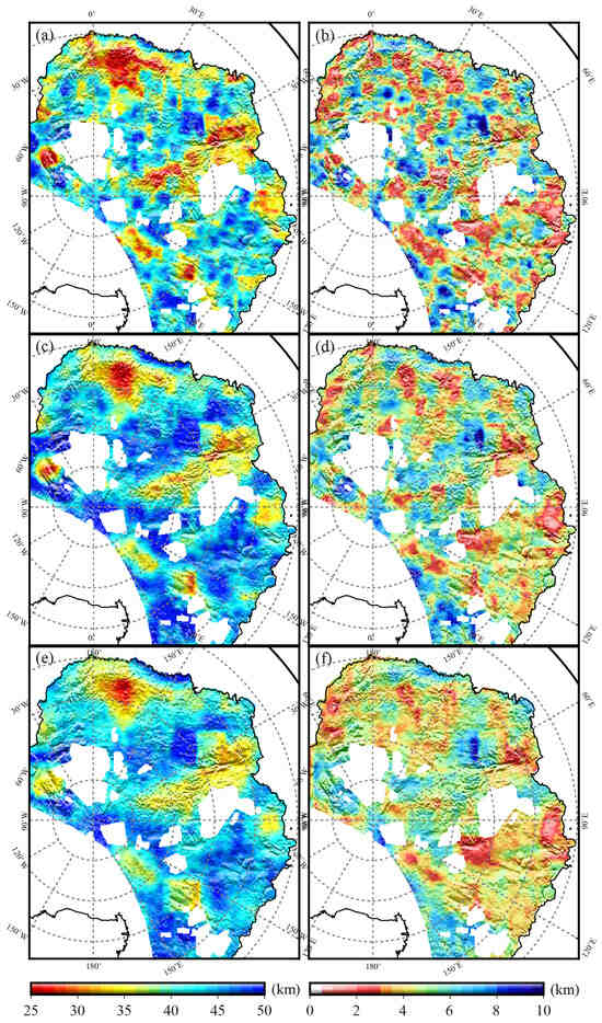
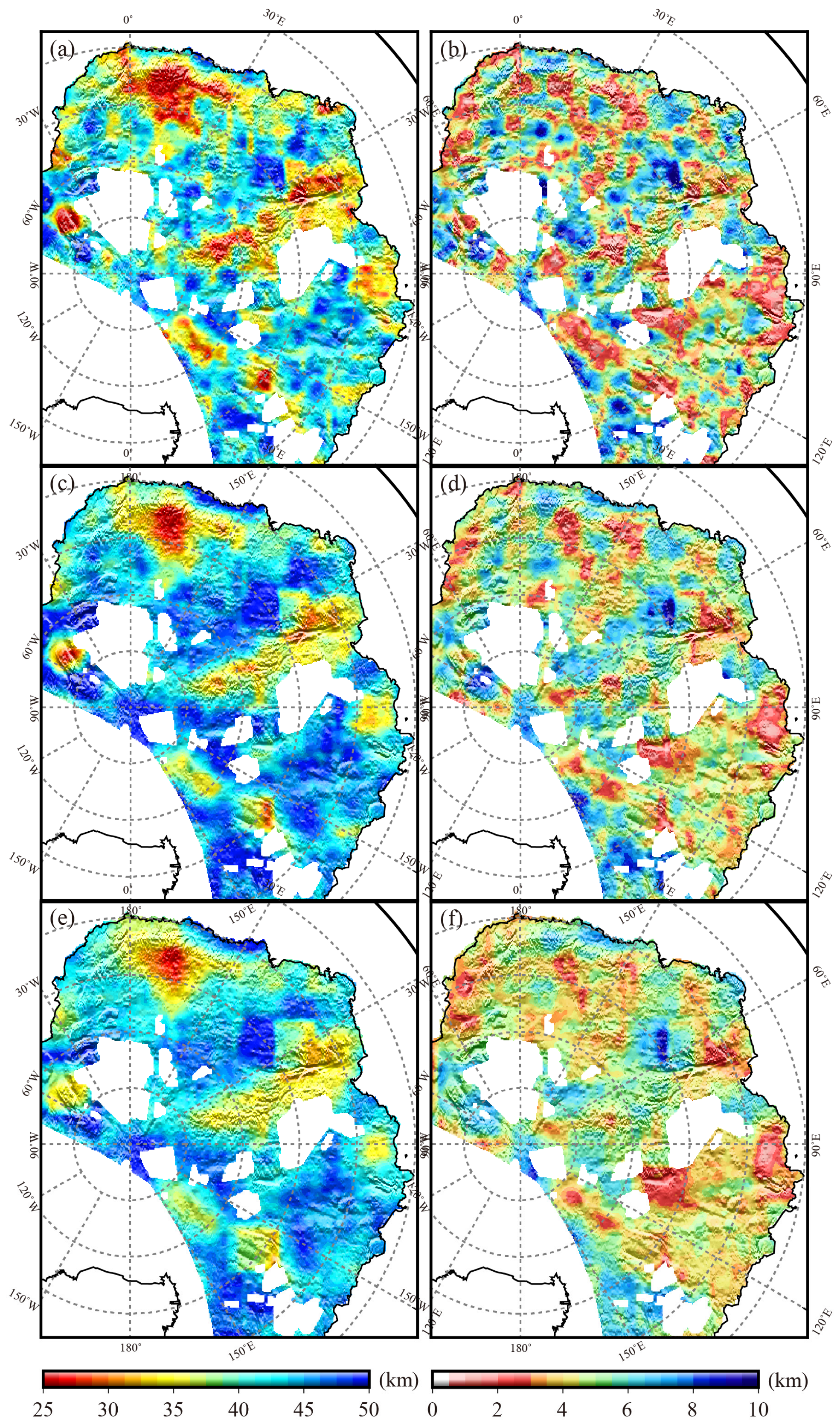
As previously pointed out, window size is a critical parameter in the estimation of Curie-point depth [28,37,38], and these studies suggested that a larger window can produce a model with poor spatial resolution, whereas a smaller window could bias the $Z_b$ values. Figure 4 shows the estimated $Z_b$ and uncertainty for three different window sizes (200 × 200, 300 × 300 and 400 × 400 km²) over the study area, with moving steps of 50 km. As we can see, the first-order patterns of spatial variation of $Z_b$ values seem to be similar among the results obtained using different windows, accompanied by only a few local differences in the study area. For example, we find that the $Z_b$ results estimated by different window sizes always display low values in Dronning Maud Land, the Gamburtsev Subglacial Mountains and the Lambert Rift, but those in the Wilkes Subglacial Basin are characterized by deep Curie-point depths. Overall, Figure 4 shows that the $Z_b$ results from 200 × 200 km² windows range from 18 km to 56 km; these values range between 20 km and 61 km and from 24 km to 57 km for 300 × 300 km² and 400 × 400 km² windowed estimates, respectively. In addition, the estimated uncertainties of $Z_b$ values decrease with growing window size, with a maximum value of 11 km at 200 × 200 km² and 9 km at 400 × 400 km². We also observe that large uncertainties occur in regions where the Curie point is very deep.

Figure 4. Maps of $Z_b$ values (a,c,e) and corresponding uncertainties (b,d,f) in East Antarctica from three different window sizes, 200 × 200 km², 300 × 300 km² and 400 × 400 km², with a constant 3D fractal exponent of 1.5.

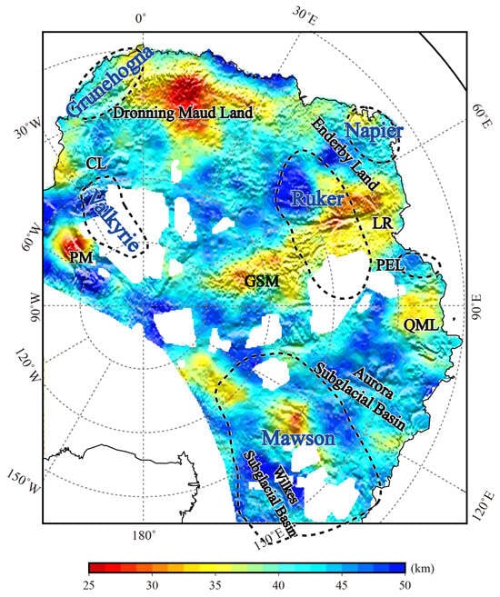
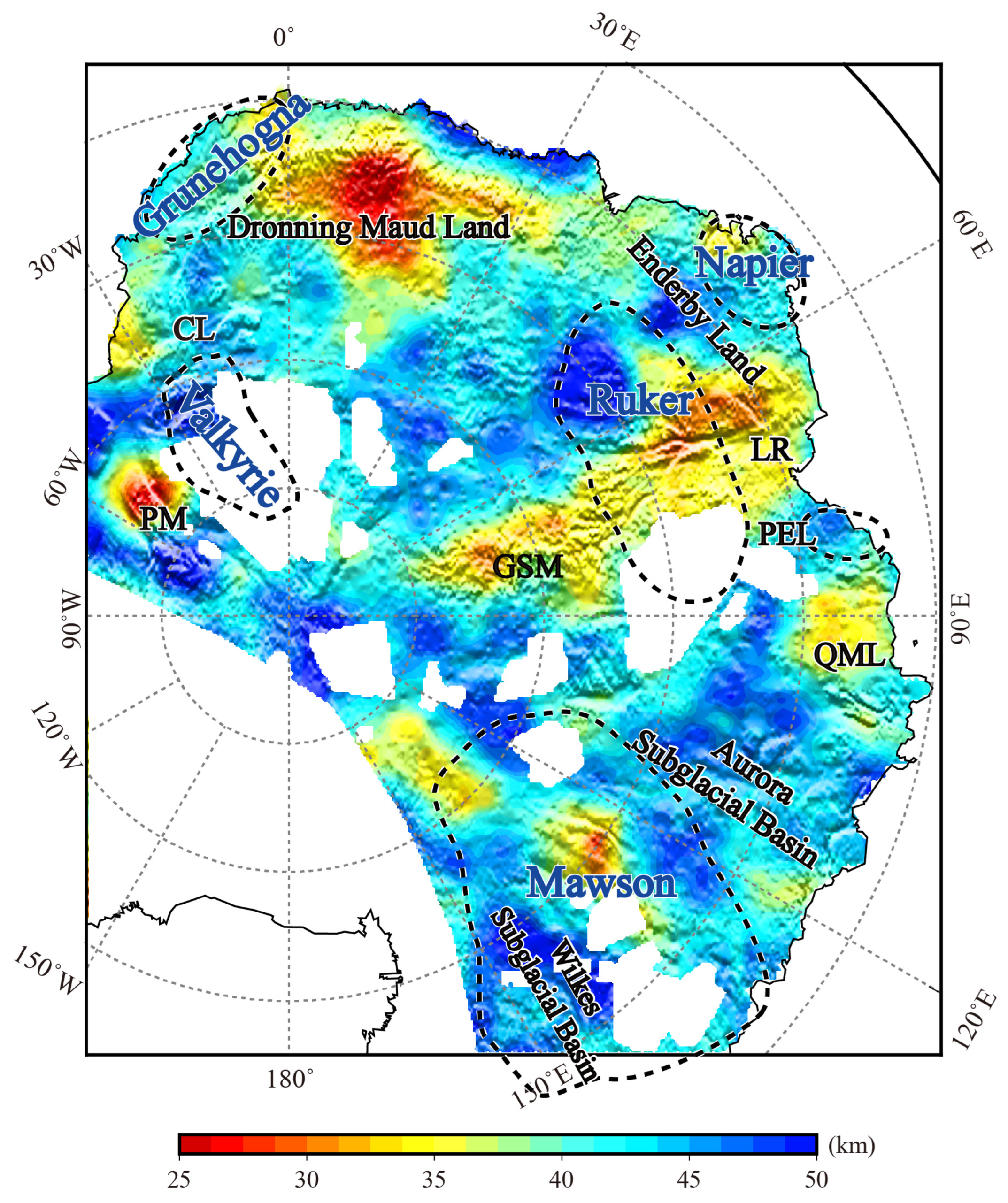
To maintain spatial resolution and validity, the ultimate model of Curie-point depth is commonly built by averaging the results from different window sizes [29,30]. As shown in Figure 5, the averaged Curie-point depth in East Antarctica exhibits high variation, with $Z_b$ values ranging from 23 to 55 km. The Gamburtsev Subglacial Mountains and Dronning Maud Land, the largest subglacial heights in East Antarctica, are characterized by a shallow Curie-point depth with a $Z_b$ value of less than 30 km. In particular, Dronning Maud Land has the shallowest $Z_b$, with a value of 23 km. The low-value pattern of $Z_b$ in the Gamburtsev Subglacial Mountains extends continually seaward to the Lambert Rift. Moreover, shallow Curie-point depths (~28–34 km) are found in Queen Mary Land and the hinterland of the Wilkes Subglacial Basin. A more pronounced shallow anomaly is also observed near the Pensacola Mountains, which geologically belong to a branch of the Transantarctic Mountains, with a $Z_b$ value lower than 30 km. This feature is distinct from the adjacent Shackleton Range and Ronne Filchner Ice Shelf. In contrast, $Z_b$ is deepest (~55 km) in the local inland area of Enderby Land, which is slightly deeper than values found in the Wilkes Subglacial Basin and Aurora Subglacial Basin, where it changes between 45 and 50 km. The South Pole region is marked by a relatively deep $Z_b$, larger than 47 km. Due to the absence of measured aeromagnetic data, the $Z_b$ values in the remaining areas of East Antarctica are not represented.

Figure 5. Averaged Curie-point depth distribution of East Antarctica from the three different window sizes described in Figure 4.

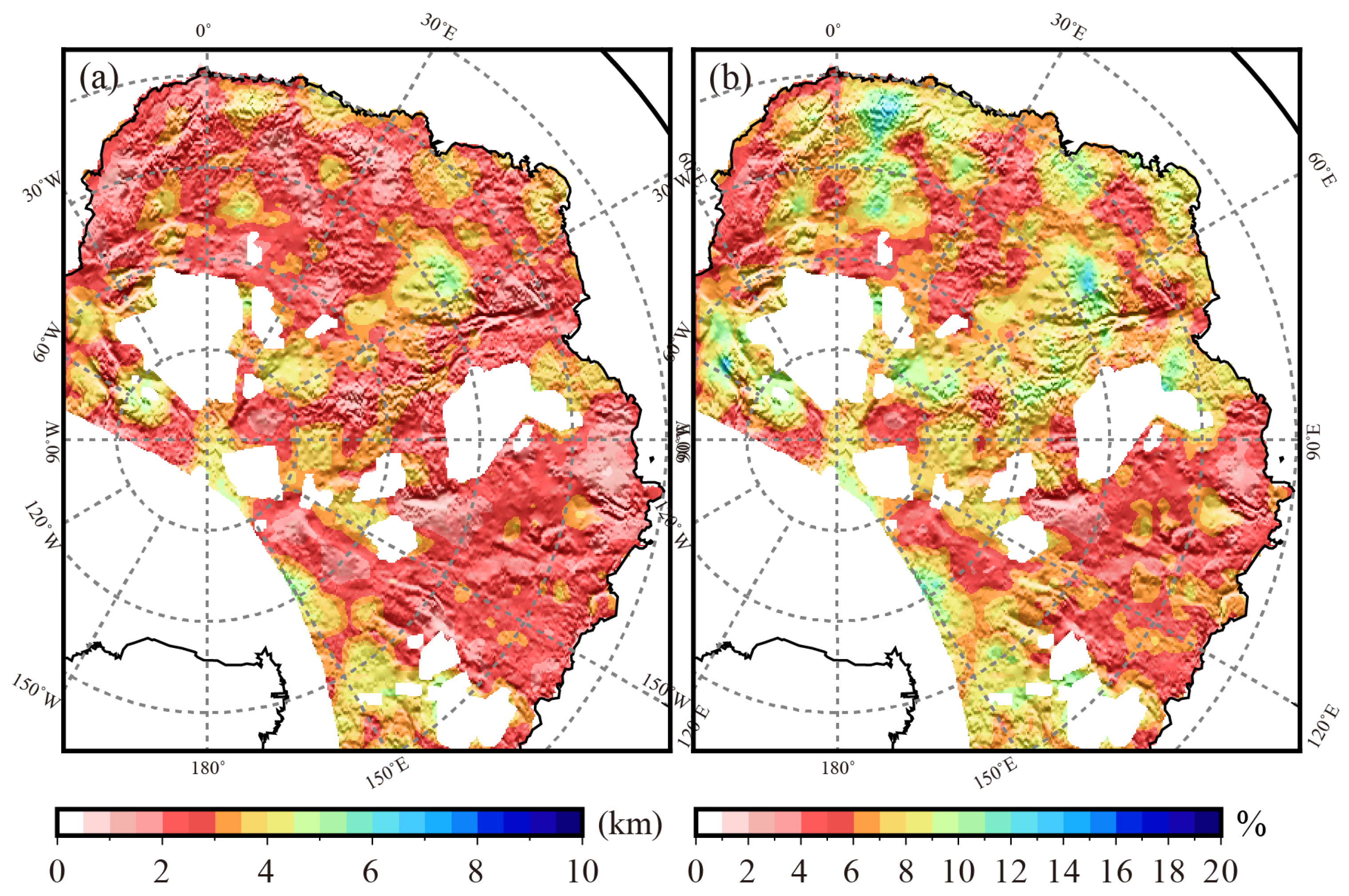
Moreover, we determined the errors in averaged $Z_b$ based on Equation (6), and they vary mostly within 3 km, with a maximum error of 5 km (Figure 6). We note that even though large $Z_b$ uncertainties occur beneath a few regions, such as the inland area of Enderby Land, our results clearly indicate that relative errors, lower than 12%, are not evident. Therefore, we suggest that $Z_b$ uncertainty does not significantly affect the final $Z_b$ values or subsequent relevant discussions.

Figure 6. The uncertainty (a) and relative error (b) of the averaged Curie-point depths of East Antarctica derived from the three different window sizes described in Figure 4.

3.2. Thermal Lithospheric Thickness

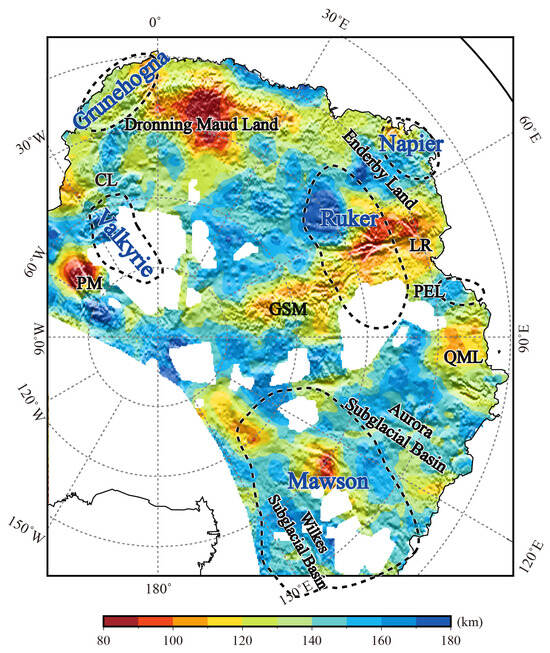
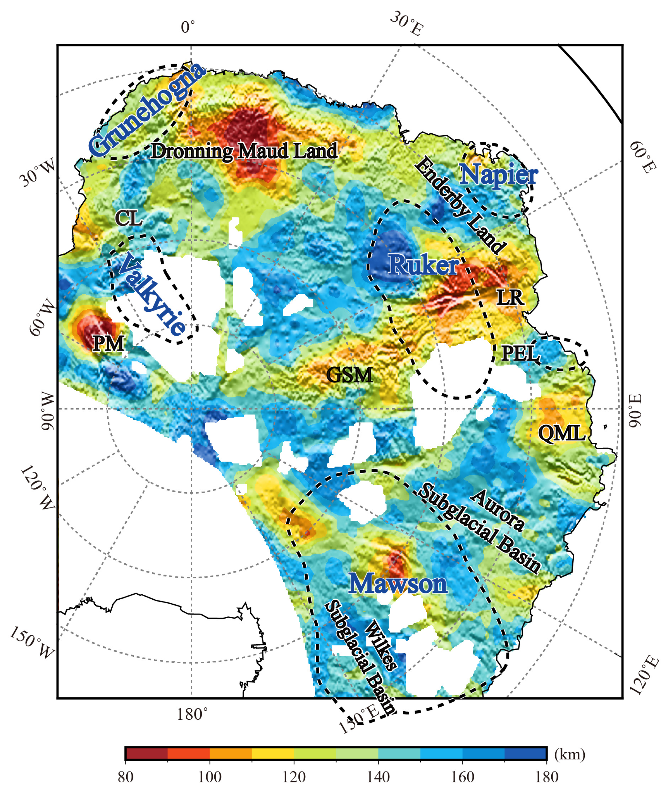
As described in Section 2.3, by assuming two thermally conductive layers and a mantle adiabat, Curie-point depths can be employed to infer thermal lithospheric thickness using Equations (7) and (8). Figure 7 illustrates the estimated thermal thickness, ranging between 70 and 200 km, which is comparable to thicknesses found in previous studies that investigated the Antarctic continent using different geophysical data, such as gravity and geoid data [18,20]. The thermal lithospheric thickness model correlates well with the tectonic provinces and their boundaries, including the preserved cratons and surrounding deformed mobile belts.

Figure 7. Distribution of calculated lithospheric thermal thicknesses of East Antarctica.

Overall, the lithospheric thickness model shows significant regional variations, and it resembles the Curie-point estimates, which is expected since the thickness is controlled by the lithospheric geotherm. Our estimates for the average of the thermal thickness range from approximately 137 km up to 200 km in the hinterland of Enderby Land. This thick lithospheric block extends towards the South Pole region, where seismic data coverage is poor. In the adjacent Gamburtsev Subglacial Mountains, Lambert Rift, and Dronning Maud Land, the lithosphere exhibits shallow depths of less than 110 km, and the thinnest lithosphere is found in Dronning Maud Land, with a depth of 70 km. The uncertainty of lithospheric thickness is calculated from the model uncertainty of $Z_b$ (Figure 6a), which represents the lower bound of total model uncertainty, shown in Figure S2 in the Supplementary File. Uncertainty varies mostly within 30 km, and the maximum uncertainty (40 km) is concentrated in the hinterland of Enderby Land, where the lithosphere is thickest.

The Wilkes and Aurora subglacial basins are also underlain by a deep anomaly with an average thermal thickness of ~155 km, which extends toward the South Pole. But in the inland area of the Wilkes Subglacial Basin, the thermal thickness decreases from approximately 140–170 km to less than 90 km. In addition, a relatively shallow thermal thickness occurs in Queen Mary Land, varying between 120 and 140 km, which is closely related to volcanic zones (e.g., Mount Gaussberg), for which elevated heat flow values were inferred by Stål [22]. Similar to the observed shallow $Z_b$ anomaly, the Pensacola Mountains are marked by a sharp change in lithospheric thickness of roughly 70 km compared to the surrounding, thicker lithosphere.

4. Discussion

4.1. Comparison with a Previous Lithospheric Thickness Model

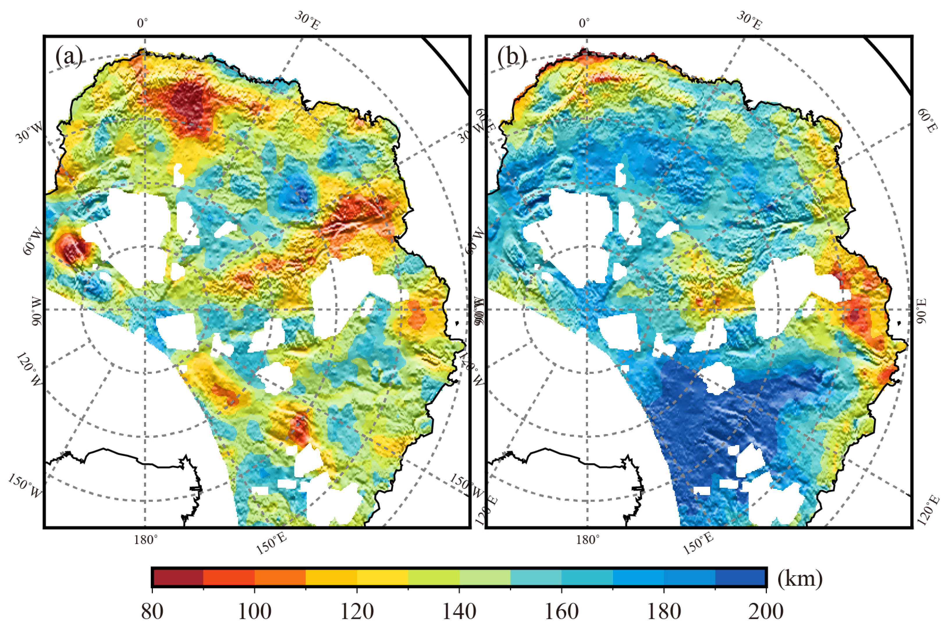
Recently, Ji et al. [20] presented a high-resolution continental-scale model of lithospheric thickness over Antarctica by joint modeling of geoid, elevation, seismically determined Moho depth data and thermal analysis. To examine the reliability of the thermal thickness model in this study, we compared our model to Ji’s model. In order to make a clear comparison, we adopted consistent data coverage for both models, and Figure 8 shows the results of the comparison. The models were developed using totally different potential field data (geoid vs. magnetic data) and inversion methods, yet they show very similar spatial patterns over most regions of East Antarctica. In most of the regions, the models have close variational ranges, within 70–200 km (Figure 8a) and 60–220 km (Figure 8b), respectively, but the magnetic-derived model in this study displays more obvious lateral variations, especially in the East Antarctic inland area, which means that the latter model displays a smoother geometry of the thermal boundary. In amplitude, they both reveal a pronounced thin lithosphere under the Gamburtsev Subglacial Mountains, Queen Mary Land, and Dronning Maud Land and a thick lithosphere in the Wilkes and Aurora subglacial basins, the inland area of Enderby Land, and the South Pole region where model uncertainty is relatively large, corresponding to cold and mechanically strong East Antarctic cratons (Figure 7). It is worth noting that the spatial extents of the above patterns derived from the two models are inconsistent. For example, the thin lithosphere features in Dronning Maud Land derived from the thermal model in this study have a larger spatial extent than those from the geoid-derived model.

Figure 8. Comparison between the calculated lithospheric thermal thickness model in this study (a) and a previous model (b) from Ji et al. [20].

By comparison, we find that large differences between the magnetic-derived and geoid-derived models occur in the Wilkes and Aurora subglacial basins, corresponding to the areas with longitudes between 90 and 150°E. A notable inconsistency can be found in the southern region of the Wilkes Subglacial Basin, with the maximum difference reaching nearly 80 km. In this region, the new thermal thickness model displays a thermal anomaly, whereas the Wilkes and Aurora subglacial basins in the geoid-derived model are dominated by a thick and cold lithosphere. Although previous seismic studies show a cratonic-like fast shear wave velocity beneath the subglacial basins of Wilkes Land (e.g., Lloyd et al. [10]), a newly developed tomographic model for East Antarctica from Hansen and Emry [39] detected a few local-scale low velocity anomalies beneath the Wilkes and Aurora subglacial basins, which are characterized by slow mantle anomalies (~5–8%). They further suggested that the Wilkes Subglacial Basin presents a Ross-aged rift reactivated by subsequent activities in the Mesozoic, suggesting that locally elevated temperatures beneath the Wilkes Subglacial Basin are possible.

Another significant inconsistency can be seen in the Lambert Rift, where an apparent thermal anomaly was detected in the magnetic-derived thermal thickness model but not in the geoid-derived model. The Lambert Rift is a failed Permian rift that extends from Prydz Bay to the hinterland of the East Antarctic Shield, which experienced multiple stages of tectonic activity, including extension and faulting, since the Permian age [2,40]. High-density materials in the lower crust were detected in the Lambert Rift using gravity modeling, which indicates the presence of large-scale magmatism in this region [41]. Combined with rifting activities and related magmatism, a thermal anomaly under the Lambert Rift seems to be more reasonable. A significant reason for the existence of inconsistencies is that the lithospheric thickness estimated in this study represents a thermal boundary at the bottom of the lithosphere, but the geoid-derived model, as shown in Figure 8b, estimates isostatic lithospheric thickness based on an assumption of local isostasy. This means that different proxies for the lithospheric thickness are considered in these two models.

4.2. Tectonics and Deep Thermal Structure in East Antarctica

Lithospheric thermal thickness (Figure 7) in East Antarctica shows a highly heterogeneous pattern, which reflects regional variations in lithospheric thermal structure. This pattern is in overall agreement with published Antarctic heat flow models [8,22], in which elevated heat flows can be found in the inland mountains of East Antarctica. Dronning Maud Land is a topographic high in East Antarctica that is characterized by an anomalously thinned and hot lithosphere, indicating a tectonically deformed zone. This pattern correlates well with other geophysical observations, such as low seismic wave velocities in the upper mantle [6,10], elevated heat flows [8], and weak lithosphere [20,42]. Based on the geochemical evidence, Jacobs et al. [43] suggested that this anomaly of a thin, hot and weak lithosphere in Dronning Maud Land is associated with delamination of the orogen root, possibly caused by the assembly of the Gondwana supercontinent in the early Paleozoic, or by a mantle plume in the Jurassic.

The low lithospheric thickness beneath the Gamburtsev region is a significant feature of the thermal structure in this study. This mountain range, with an elevation of more than 3000 m, is situated in the middle of East Antarctica and has a poorly understood formation process caused by its complex lithospheric structure [5,20]. Previous seismic studies indicate a thick (>250 km) and high-velocity cratonic lithosphere beneath the Gamburtsev Subglacial Mountains [6,44]. However, our results, surprisingly, show the presence of a thinned lithosphere (~100–110 km) beneath this area, which is consistent with the recent findings of our geoid study [20] (Figure 8). They interpret this pattern as the result of thermally related lithospheric modification in the post-orogenic process, which is supported by the extremely low lithospheric strength in the Gamburtsev Subglacial Mountains [20,42,45]. This feature could be possible, since recent seismic tomographic results also do not show a thick lithosphere beneath this portion of East Antarctica. Shen et al. [46] generated a model of the crustal and upper mantle structure across Central and West Antarctica by jointly inverting the Rayleigh wave phase and group velocity with P wave receiver functions, and a reduced S-velocity pattern at a depth of 50 to 120 km was imaged beneath the Gamburtsev Subglacial Mountains. They hypothesized that this anomaly was the result of mantle eclogitization, possibly because of continental collision or subduction rather than a thermal anomaly. Furthermore, the regional shear-wave velocity structure of the Gamburtsev crust was investigated by Huang et al. [47], and low-velocity crustal anomalies were observed in their tomographic model. They further attributed these anomalies to fault systems and decompression melting in the upper mantle, which, together with the thick crust, maintain the high elevation of this mountain range. Haeger et al. [8] converted the global tomography model into a temperature model over Antarctica, and they found an elevated heat flow and thinned lithosphere beneath Gamburtsev, which are similar in pattern to the seismically inferred temperature profiles of Hazzard et al. [48]. Additionally, Haeger et al. [49] explored the 3D temperature structure of the Antarctic lithosphere by combining mineral physics and data of gravity, and seismic tomography, and they discovered a high-temperature anomaly in the upper mantle of the Gamburtsev region with an amplitude reaching a maximum value of 1050 °C at a depth of 100 km. Likewise, our previous geoid study indicated a high Moho temperature in this mountain region [20].

Thus, similar to the results in this study, the new seismic models, seismic- and potential-field-constrained thermal studies contradict previous seismically determined results that suggest a cold craton with a super-thick lithospheric root [6,44]. Given the fact that multiple periods of tectonic activity affected the Gamburtsev lithosphere, including collisional events associated with Gondwana’s assembly and the rifting that followed [1,40,50], we infer that the lithosphere of this mountain range could have been thermally reworked during post-collisional tectonic events related to the assembly and breakup of the Gondwana supercontinent. These tectonothermal events led to the reduced seismic velocity and strength of the Gamburtsev lithosphere and to elevated heat flow values. Based on the above-mentioned geophysical features, a thinned lithosphere in this region is highly possible, and we prefer the hypothesis of an anomalously warm lithosphere beneath the Gamburtsev Subglacial Mountains, which may be responsible for supporting its high topography. As for the heat source beneath this mountain range, we cannot determine from the observed steep geothermal gradient and shallow depth of the Curie-temperature isotherm alone whether the thermal anomalies derive from the shallow crust or the underlying lithospheric mantle. Hazzard et al. [48] explained the high heat flow anomaly over the Gamburtsev crust in their model as the result of high crustal radiogenic heat production within the crust, since this area has a super-thick crust. However, Li and Aitken [51] developed a crustal radiogenic heat production model by applying empirical relationships with crustal density, and the results show that there is no pronounced increase in heat production in the Gamburtsev crust. Consequently, we suggest that the thermal anomalies may derive from deep lithospheric mantle sources that conduct heat to the uppermost crust.

Moreover, a local short-wavelength thermal anomaly, with a diameter of 400 km, surrounded by thick lithosphere is restricted to the area of the Pensacola Mountains, which corresponds to negative magnetic anomalies (Figure 2). This thermal anomaly represents a previously unrecognized thin lithosphere, and it is similar in amplitude to the thinned lithosphere in Dronning Maud Land. One likely reason is that due to the small size of the Pensacola Mountains anomaly, it could not be resolved by seismic tomography studies. The Pensacola Mountains are located at the easternmost end of the Transantarctic Mountains, and geological evidence shows that the Pensacola Mountains formed during the Ross orogeny [52,53]. Considering that the Pensacola Mountains lie near the Weddell Sea Rift System, it would appear that the lithosphere of the Pensacola Mountains may have experienced thermal modification in the following tectonothermal events, such as magmatism during the opening of the Weddell Sea in the Jurassic [54].

Archean cratons have generally strong cratonic roots with high viscosity that increase their longevity [55]. In the East Antarctic Shield, several cratons may have been preserved as continental fragments in the present-day lithosphere, characterized by high strength and low temperature. Considering their cold thermal state, we can roughly utilize the variations in our thermal thickness (Figure 7) to analyze the distribution of cratonic blocks. We found that the spatial extent of the thick lithosphere in the Wilkes and Aurora subglacial basins, extending westward to the boundary of Queen Mary Land, is larger than the delineated Mawson Craton. But local-scale thermal anomalies occur in the cratonic interior, suggesting that this large-sized craton in East Antarctica contains strongly deformed blocks at the center of this region, and that the Mawson Craton could have experienced a certain degree of lithospheric deformation and lose its integrated cratonic signature. This spatial feature is consistent with the results of lithospheric strength analysis, which shows that a few fragments with moderate strength values are located in the Wilkes Subglacial Basin [42]. In contrast, a thick lithospheric block is only observed in the western region of the Lambert Rift, which indicates that the Ruker Craton cannot be as large as previously suggested [3,20]. Also, our thermal thickness model shows that the Ruker Craton extends southward to 85°S, and we suggest that this craton may extend in the north–south direction rather than in the east–west direction. Napier Complex and Grunehogna Craton are two Archean blocks situated at the continental margin that are lower than the Ruker Craton in amplitude, which implies that they may have experienced thermal perturbation during the Gondwana breakup.

5. Conclusions

In this study, using newly published aeromagnetic data, we employed the wavenumber-domain centroid method to estimate Curie-point depths in East Antarctica, which we used to infer thermal lithospheric thickness by combining the 1D steady thermal conductivity data. Compared to previous studies that used seismic, gravity and geoid data, our findings provide independent constraints on lithospheric thickness beneath East Antarctica.

We demonstrated a strongly heterogeneous lithospheric thermal structure in East Antarctica. We identified two distinct thermal anomalies with lithospheric thicknesses of 100–110 km and 70–110 km beneath the Gamburtsev Subglacial Mountains and Dronning Maud Land, respectively, whose existence is supported by previous geoid and seismic studies. In addition, our thermal thickness model unveils other small-scale features, including a local-scale thinned lithosphere in the Pensacola Mountains. Ultimately, we found that a few cratons within East Antarctica may have lost their roots.

References

- Fitzsimons, I.C.W. Grenville-age basement provinces in East Antarctica: Evidence for three separate collisional orogens. Geology 2000, 28, 879–882. [Google Scholar] [CrossRef] [Scilit]
- Ferraccioli, F.; Finn, C.A.; Jordan, T.A.; Bell, R.E.; Anderson, L.M.; Damaske, D. East Antarctic rifting triggers uplift of the Gamburtsev Mountains. Nature 2011, 479, 388–392. [Google Scholar] [CrossRef] [Scilit]
- Jordan, T.A.; Ferraccioli, F.; Forsberg, R. An embayment in the East Antarctic basement constrains the shape of the Rodinian continental margin. Commun. Earth Environ. 2022, 3, 52. [Google Scholar] [CrossRef] [Scilit]
- Morlighem, M.; Rignot, E.; Binder, T.; Blankenship, D.; Drews, R.; Eagles, G.; Eisen, O.; Ferraccioli, F.; Forsberg, R.; Fretwell, P.; et al. Deep glacial troughs and stabilizing ridges unveiled beneath the margins of the Antarctic ice sheet. Nat. Geosci. 2020, 13, 132–137. [Google Scholar] [CrossRef] [Scilit]
- Burton-Johnson, A.; Dziadek, R.; Martin, C. Geothermal heat flow in Antarctica: Current and future directions. Cryosphere 2020, 14, 3843–3873. [Google Scholar] [CrossRef] [Scilit]
- An, M.; Wiens, D.; Zhao, Y.; Feng, M.; Nyblade, A.; Kanao, M.; Li, Y.; Maggi, A.; Lévêque, J.-J. Temperature, lithosphere-asthenosphere boundary, and heat flux beneath the Antarctic Plate inferred from seismic velocities. J. Geophys. Res. Solid Earth 2015, 120, 8720–8742. [Google Scholar] [CrossRef] [Scilit]
- Shen, W.; Wiens, D.; Lloyd, A.; Nyblade, A. A geothermal heat flux map of Antarctica empirically constrained by seismic structure. Geophys. Res. Lett. 2020, 47, e2020GL086955. [Google Scholar] [CrossRef] [Scilit]
- Haeger, C.; Petrunin, A.G.; Kaban, M.K. Geothermal heat flow and thermal structure of the Antarctic lithosphere. Geochem. Geophys. Geosyst. 2022, 23, e2022GC010501. [Google Scholar] [CrossRef] [Scilit]
- Wiens, D.A.; Shen, W.S.; Lloyd, A.J. The seismic structure of the Antarctic upper mantle. Geol. Soc. Lond. Mem. 2023, 56, 195–212. [Google Scholar] [CrossRef] [Scilit]
- Lloyd, A.J.; Wiens, D.A.; Zhu, H.; Tromp, J.; Nyblade, A.A.; Aster, R.C.; Hansen, S.E.; Dalziel, I.W.; Wilson, T.J.; Ivins, E.R.; et al. Seismic structure of the Antarctic upper mantle imaged with adjoint tomography. J. Geophys. Res. Solid Earth 2020, 125. [Google Scholar] [CrossRef] [Scilit]
- Brown, S.; Fischer, K. Investigating the Antarctic lithosphere through Sp receiver function analysis. Geochem. Geophys. Geosyst. 2025, 26, e2025GC012268. [Google Scholar] [CrossRef] [Scilit]
- Fox Maule, C.; Purucker, M.E.; Olsen, N.; Mosegaard, K. Heat Flux Anomalies in Antarctica Revealed by Satellite Magnetic Data. Science 2005, 309, 464–467. [Google Scholar] [CrossRef] [Scilit]
- Martos, Y.; Catalán, M.; Jordan, T.A.; Golynsky, A.; Golynsky, D.; Eagles, G.; Vaughan, D.G. Heat flux distribution of Antarctica unveiled. Geophys. Res. Lett. 2017, 44, 11417–11426. [Google Scholar] [CrossRef] [Scilit]
- Li, L.; Tang, X.; Guo, J.; Cui, X.; Xiao, E.; Latif, K.; Sun, B.; Zhang, Q.; Shi, X. Inversion of Geothermal Heat Flux under the Ice Sheet of Princess Elizabeth Land, East Antarctica. Remote Sens. 2021, 13, 2760. [Google Scholar] [CrossRef] [Scilit]
- Wu, G.; Ferraccioli, F.; Zhou, W.; Yuan, Y.; Gao, J.; Tian, G. Tectonic Implications for the Gamburtsev Subglacial Mountains, East Antarctica, from Airborne Gravity and Magnetic Data. Remote Sens. 2023, 15, 306. [Google Scholar] [CrossRef] [Scilit]
- Lowe, M.; Mather, B.; Green, C.; Jordan, T.; Ebbing, J.; Larter, R. Anomalously high heat flow regions beneath the Transantarctic Mountains and Wilkes subglacial basin in East Antarctica inferred from curie depth. J. Geophys. Res. Solid Earth 2023, 128, e2022JB025423. [Google Scholar] [CrossRef] [Scilit]
- Pappa, F.; Ebbing, J.; Ferraccioli, F.; van der Wal, W. Modeling satellite gravity gradient data to derive density, temperature, and viscosity structure of the Antarctic lithosphere. J. Geophys. Res. Solid Earth 2019, 124, 12053–12076. [Google Scholar] [CrossRef] [Scilit]
- Artemieva, I.M. Antarctica ice sheet basal melting enhanced by high mantle heat. Earth Sci. Rev. 2022, 226, 103954. [Google Scholar] [CrossRef] [Scilit]
- Afonso, J.C.; Fullea, J.; Griffin, W.L.; Yang, Y.; Jones, A.G.; Connolly, J.A.D.; O’Reilly, S.Y. 3-D multiobservable probabilistic inversion for the compositional and thermal structure of the lithosphere and upper mantle. I: A priori petrological information and geophysical observables. J. Geophys. Res. Solid Earth 2013, 118, 2586–2617. [Google Scholar] [CrossRef] [Scilit]
- Ji, F.; Xu, M.; Zhang, Q.; Liu, X.; Zhou, X. Lithospheric structure and strength variations in Antarctica from joint modeling of elevation, geoid and seismic data. J. Geophys. Res. Solid Earth 2024, 129, e2024JB029455. [Google Scholar] [CrossRef] [Scilit]
- Lösing, M.; Ebbing, J. Predicting geothermal heat flow in Antarctica with a machine learning approach. J. Geophys. Res. Solid Earth 2021, 126, e2020JB021499. [Google Scholar] [CrossRef] [Scilit]
- Stål, T.; Reading, A.M.; Halpin, J.A.; Whittaker, J.M. Antarctic geothermal heat flow model: Aq1. Geochem. Geophys. Geosyst. 2021, 22, e2020GC009428. [Google Scholar] [CrossRef] [Scilit]
- Chu, D.; Fan, X.; Li, J.; Bai, L.; Wang, Z.; Guo, J. Prediction of geothermal heat flow in Antarctica based on deep neural network. Rev. Geophys. Planet. Phys. 2026, 57, 177–190. (In Chinese) [Google Scholar] [CrossRef]
- Thébault, E.; Purucker, M.; Whaler, K.A.; Langlais, B.; Sabaka, T.J. The Magnetic Field of the Earth’s Lithosphere. Space Sci. Rev. 2010, 155, 95–127. [Google Scholar] [CrossRef] [Scilit]
- Tselentis, G.A. An attempt to define curie point depths in Greece from aeromagnetic and heat flow data. Pure Appl. Geophys. 1991, 136, 87–101. [Google Scholar] [CrossRef] [Scilit]
- Kim, H.R.; Golynsky, A.V.; Golynsky, D.A.; Leftwich, T.E.; von Frese, R.R.B.; Hong, J.K.; Lee, M. Antarctic magnetic anomalies and their gradients differentially reduced to the geomagnetic pole for enhanced crustal analysis. J. Geophys. Res. Solid Earth 2025, 130, e2024JB029687. [Google Scholar] [CrossRef] [Scilit]
- Eagles, G.; Golynsky, A.V.; Kim, H.R.; Paxman, G.; Ferraccioli, F. ADMAP’s Antarctic magnetic anomaly grids transformed for use with open source software [dataset]. PANGAEA 2024. [Google Scholar] [CrossRef]
- Li, C.; Wang, J.; Lin, J.; Wang, T. Thermal evolution of the North Atlantic lithosphere: New constraints from magnetic anomaly inversion with a fractal magnetization model. Geochem. Geophys. Geosyst. 2013, 14, 5078–5105. [Google Scholar] [CrossRef] [Scilit]
- Wang, J.; Li, C. Crustal magmatism and lithospheric geothermal state of western North America and their implications for a magnetic mantle. Tectonophysics 2015, 638, 112–125. [Google Scholar] [CrossRef] [Scilit]
- Wang, J.; Li, C. Curie point depths in northeast China and their geothermal implications for the Songliao Basin. J. Asian Earth Sci. 2018, 163, 177–193. [Google Scholar] [CrossRef] [Scilit]
- Gaudreau, É.; Audet, P.; Schneider, D.A. Mapping Curie depth across western Canada from a wavelet analysis of magnetic anomaly data. J. Geophys. Res. Solid Earth 2019, 124, 4365–4385. [Google Scholar] [CrossRef] [Scilit]
- Sobh, M.; Gerhards, C.; Fadel, I.; Gotze, H.-J. Mapping the thermal structure of southern Africa from Curie depth estimates based on wavelet analysis of magnetic data with uncertainties. Geochem. Geophys. Geosyst. 2021, 22, e2021GC010041. [Google Scholar] [CrossRef] [Scilit]
- Okubo, Y.; Matsunaga, T. Curie point depth in northeast Japan and its correlation with regional thermal structure and seismicity. J. Geophys. Res. Solid Earth 1994, 99, 22363–22371. [Google Scholar] [CrossRef] [Scilit]
- Turcotte, D.L.; Schubert, G. Geodynamics; Cambridge University Press: Cambridge, UK, 2002. [Google Scholar]
- Xu, Y.; Shankland, T.J.; Linhardt, S.; Rubie, D.C.; Langenhorst, F.; Klasinski, K. Thermal diffusivity and conductivity of olivine, wadsleyite and ringwoodite to 20 Gpa and 1373 K. Phys. Earth Planet. Inter. 2004, 143–144, 321–336. [Google Scholar] [CrossRef]
- Li, C.F.; Wang, J.L.; Zhou, Z.Y.; Geng, J.H.; Chen, B.; Yang, F.L.; Wu, J.S.; Yu, P.; Zhang, X.B.; Zhang, S.W. 3D geophysical characterization of the Sulu–Dabie orogen and its environs. Phys. Earth Planet. Inter. 2012, 192, 35–53. [Google Scholar] [CrossRef] [Scilit]
- Li, C.F.; Lu, Y.; Wang, J. A global reference model of Curie-point depths based on EMAG2. Sci. Rep. 2017, 7, 45129. [Google Scholar] [CrossRef] [Scilit]
- Li, C. An integrated geodynamic model of the Nankai subduction zone and neighboring regions from geophysical inversion and modeling. J. Geodyn. 2011, 51, 64–80. [Google Scholar] [CrossRef] [Scilit]
- Hansen, S.E.; Emry, E.L. East Antarctic tectonic basin structure and its implications for ice-sheet modeling and sea-level projections. Commun. Earth Environ. 2025, 6, 138. [Google Scholar] [CrossRef] [Scilit]
- Harrowfield, M.; Holdgate, G.R.; Wilson, C.J.L.; McLoughlin, S. Tectonic significance of the Lambert graben, East Antarctica: Reconstructing the Gondwanan rift. Geology 2005, 33, 197–200. [Google Scholar] [CrossRef] [Scilit]
- Mishra, D.C.; Chandra Sekhar, D.V.; Venkata Raju, D.C.; Vijaya Kumar, V. Crustal structure based on gravity-magnetic modelling constrained from seismic studies under Lambert Rift, Antarctica and Godavari and Mahanadi rifts, India and their interrelationship. Earth Planet. Sci. Lett. 1999, 172, 287–300. [Google Scholar] [CrossRef] [Scilit]
- Swain, C.J.; Kirby, J.F. Effective elastic thickness map reveals subglacial structure of East Antarctica. Geophys. Res. Lett. 2021, 48, e2020GL091576. [Google Scholar] [CrossRef] [Scilit]
- Jacobs, J.; Bingen, B.; Thomas, R.J.; Bauer, W.; Wingate, M.T.; Feitio, P. Early Palaeozoic orogenic collapse and voluminous latetectonic magmatism in Dronning Maud land and Mozambique: Insights into the partially delaminated orogenic root of the East African–Antarctic Orogen? Geol. Soc. Lond. Spec. Publ. 2008, 308, 69–90. [Google Scholar] [CrossRef] [Scilit]
- Lloyd, A.J.; Nyblade, A.A.; Wiens, D.A.; Hansen, S.E.; Kanao, M.; Shore, P.J.; Zhao, D. Upper mantle seismic structure beneath central East Antarctica from body wave tomography: Implications for the origin of the Gamburtsev Subglacial Mountains. Geochem. Geophys. Geosyst. 2013, 14, 902–920. [Google Scholar] [CrossRef] [Scilit]
- Paxman, G.J.G.; Watts, A.B.; Ferraccioli, F.; Jordan, T.A.; Bell, R.E.; Jamieson, S.S.R.; Finn, C.A. Erosion-driven uplift in the Gamburtsev Subglacial Mountains of east antarctica. Earth Planet. Sci. Lett. 2016, 452, 1–14. [Google Scholar] [CrossRef] [Scilit]
- Shen, W.; Wiens, D.A.; Anandakrishnan, S.; Aster, R.C.; Gerstoft, P.; Bromirski, P.D.; Hansen, S.E.; Dalziel, I.W.; Heeszel, D.S.; Huerta, A.D.; et al. The crust and upper mantle structure of central and West Antarctica from Bayesian inversion of Rayleigh wave and receiver functions. J. Geophys. Res. Solid Earth 2018, 123, 7824–7849. [Google Scholar] [CrossRef] [Scilit]
- Huang, X.; Hao, W.; Li, F.; Yao, H.; Chen, Y.; Li, D.; Yan, P. Crustal velocity imaging of the Gamburtsev Subglacial Mountains, Antarctica, based on ambient seismic noise. J. Geophys. Res. Solid Earth 2025, 130, e2024JB031047. [Google Scholar] [CrossRef] [Scilit]
- Hazzard, J.A.N.; Richards, F.D.; Goes, S.D.B.; Roberts, G.G. Probabilistic assessment of Antarctic thermomechanical structure: Impacts on Ice Sheet stability. J. Geophys. Res. Solid Earth 2023, 128, e2023JB026653. [Google Scholar] [CrossRef] [Scilit]
- Haeger, C.; Kaban, M.K.; Tesauro, M.; Petrunin, A.G.; Mooney, W.D. 3-D density, thermal, and compositional model of the Antarctic lithosphere and implications for its evolution. Geochem. Geophys. Geosyst. 2018, 20, 688–707. [Google Scholar] [CrossRef] [Scilit]
- Liu, X.; Hu, J.; Zhao, Y.; Lou, Y.; Wei, C.; Liu, X. Late Neoproterozoic/Cambrian high-pressure mafic granulites from the Grove Mountains, East Antarctica: P-T-t path, collisional orogeny and implications for assembly of East Gondwana. Precambrian Res. 2009, 174, 181–199. [Google Scholar] [CrossRef] [Scilit]
- Li, L.; Aitken, A.R.A. Crustal heterogeneity of Antarctica signals spatially variable radiogenic heat production. Geophys. Res. Lett. 2024, 51, e2023GL106201. [Google Scholar] [CrossRef] [Scilit]
- Storey, B.C.; Macdonald, D.I.M.; Dalziel, I.W.D.; Isbell, J.L.; Millar, I.L. Early Paleozoic sedimentation, magmatism, and deformation in the Pensacola Mountains, Antarctica: The significance of the Ross orogeny. GSA Bull. 1996, 108, 685–707. [Google Scholar] [CrossRef] [Scilit]
- Curtis, M.L.; Millar, I.L.; Storey, B.C.; Fanning, M. Structural and geochronological constraints of early Ross orogenic deformation in the Pensacola Mountains, Antarctica. GSA Bull. 2004, 116, 619–636. [Google Scholar] [CrossRef] [Scilit]
- Jordan, T.A.; Ferraccioli, F.; Leat, P.T. New geophysical compilations link crustal block motion to Jurassic extension and strike-slip faulting in the Weddell Sea Rift System of West Antarctica. Gondwana Res. 2017, 42, 29–48. [Google Scholar] [CrossRef] [Scilit]
- Sengör, A.M.C. Continental interiors and cratons: Any relation? Tectonophysics 1999, 305, 1–42. [Google Scholar] [CrossRef] [Scilit]
Disclaimer/Publisher’s Note: The statements, opinions and data contained in all publications are solely those of the individual author(s) and contributor(s) and not of MDPI and/or the editor(s). MDPI and/or the editor(s) disclaim responsibility for any injury to people or property resulting from any ideas, methods, instructions or products referred to in the content. |
© 2026 by the authors. Licensee MDPI, Basel, Switzerland. This article is an open access article distributed under the terms and conditions of the Creative Commons Attribution (CC BY) license.