


Highlights
What are the main findings?
- Eight distinct vegetation structural types across 370,000 ha of arid and semi-arid rangelands were identified and mapped using high-density aerial LiDAR.
- Unsupervised fuzzy c-means classification allowed for quantifying mapping confidence for each pixel.
What are the implications of the main findings?
- We revealed previously unknown vegetation structural heterogeneity in the study area.
- The vegetation structural maps presented here are a baseline for rangeland ecological condition assessments and a key input for rangeland management and restoration planning.
Abstract
Rangelands occupy over half of the Earth’s terrestrial surface and play an important role in supporting biodiversity and livelihoods. However, widespread degradation—particularly in arid and semi-arid regions—has compromised their ecological function. Traditional monitoring approaches that rely on vegetation cover metrics from optical satellite imagery fail to capture the three-dimensional structure of vegetation, which is critical for assessing ecosystem condition and guiding restoration and management efforts. This study demonstrates the application of high-density airborne LiDAR (ALS) data (~15–20 points/m2) to identify and map vegetation structural types across 370,000 hectares of semi-arid rangelands in Western Australia. Using an unsupervised fuzzy c-means clustering algorithm on seven minimally correlated ALS-derived structural metrics, we identified eight statistically distinct vegetation structural classes. The resulting structural map revealed spatial heterogeneity in vegetation structure, including in areas with similar vegetation cover, with high confidence in structural attribution in 74.5% of the study area. The rangeland-specific structural classes developed in this study, which incorporate measures of classification certainty, offer a robust framework for vegetation structural mapping in field data-scarce environments. This framework can support ecological condition assessments and provide a basis for rangeland management and restoration planning.
1. Introduction
Rangelands cover over half of Earth’s terrestrial surface and support nearly one-third of the global population while maintaining high biodiversity [1,2]. Despite this importance, approximately 50% of global rangelands show evidence of degradation driven largely by anthropogenic pressures, particularly in arid and semi-arid regions [3]. In Australia, pastoral overgrazing since European settlement has led to substantial soil erosion and vegetation decline [4], yet the spatial extent and severity of these impacts remain poorly quantified. Effective monitoring of such vast and heterogeneous landscapes requires approaches that capture vegetation characteristics at ecologically meaningful scales.
Current monitoring programs rely primarily on vegetation cover metrics from optical satellite imagery [5,6,7]. While cover is useful for detecting broad patterns of change, it cannot distinguish structurally distinct vegetation types that share similar cover values. For example, degraded shrublands and intact open woodlands may exhibit comparable overall cover but differ markedly in habitat quality, carbon storage, and resilience to disturbance [8,9]. Vegetation structure—the three-dimensional arrangement of biomass—offers insights into these functional differences, yet structural information is largely unmapped across most rangeland regions.
Structural diversity influences wildlife habitats [10], ecosystem service provision [11], and carbon sequestration [12]. Rangeland vegetation spans grasslands, shrublands, and woodlands [13], with structural variation shaped by disturbance history, soil properties, and climatic gradients. Mapping this variation is essential for assessing ecological condition and guiding management interventions, particularly where degradation is spatially patchy and restoration potential varies across landscapes. Management actions, such as herbivory reduction or interventions to enhance water infiltration, may have different outcomes depending on existing vegetation structure [14].
Airborne laser scanning (ALS) allows to characterise structure at fine spatial resolution. Although widely applied in forests, ALS use in rangelands remains limited [15,16]. Previous studies have relied on low-density ALS data and predefined structural classes, yielding moderate accuracy [17,18]. These approaches impose a priori assumptions about which structural types should be present and are further constrained by the inability of low-density point clouds to detect sparse or low-stature vegetation typical of arid systems. Consequently, structurally distinct vegetation states may remain unresolved, and transitional or degraded forms may be forced into ill-fitting categories.
More recently available high-density ALS datasets offer new opportunities to overcome these limitations. Increased point densities enable detection of subtle vertical features and sparse vegetation elements that are often missed in coarser surveys, supporting more detailed characterisation of rangeland structure. However, exploiting this information requires classification approaches that do not depend on predefined structural classes, particularly in regions where degradation has altered vegetation associations in ways that are difficult to define a priori.
There are multiple analytical pathways for deriving vegetation structural types from ALS data. Supervised machine-learning methods (e.g., maximum likelihood, k-NN, random forest, boosted regression trees, and support vector machines) are commonly used when vegetation groups are well defined, and sufficient training data exist [19]. In contrast, unsupervised classification approaches are more appropriate when the objective is to discover emergent structural patterns rather than map known classes, especially in areas with limited field data. This is especially relevant in degraded rangelands, where novel or transitional vegetation structures may occur. Among unsupervised methods, k-means clustering has been applied successfully across a range of ecosystems [20,21,22], yet this method assigns each observation exclusively to a single class and provides no measure of classification uncertainty. Fuzzy c-means clustering [23] extends this framework by allowing partial membership across multiple classes, explicitly representing ambiguity and gradual structural transitions. This capability is particularly suited to rangeland environments, where vegetation boundaries are often diffuse and mixed structural states are common. Importantly, fuzzy clustering enables spatially explicit mapping of classification uncertainty, information that is rarely reported in rangeland vegetation structure studies but is highly relevant for management and restoration planning.
The southern rangelands of Western Australia exemplify the need for improved structural mapping. Existing classification systems and field-based assessments [24,25] offer valuable regional descriptions but are labour-intensive and spatially limited. Integrating high-density ALS with environmental data can reveal where vegetation structure deviates from expected conditions, identifying areas with high restoration potential.
This study used high-density ALS to map vegetation structural types across Western Australian rangelands using unsupervised classification. Our objectives were to: (1) identify structural classes using fuzzy c-means clustering of ALS metrics at a 1 ha scale; (2) validate classes using statistical separability and photo-interpretation; and (3) map classification uncertainty. We hypothesised that high-density ALS would reveal previously unrecognised structural heterogeneity relevant to rangeland management.
2. Materials and Methods
2.1. Study Area
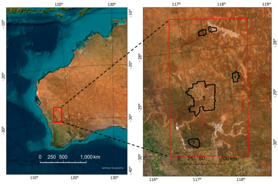
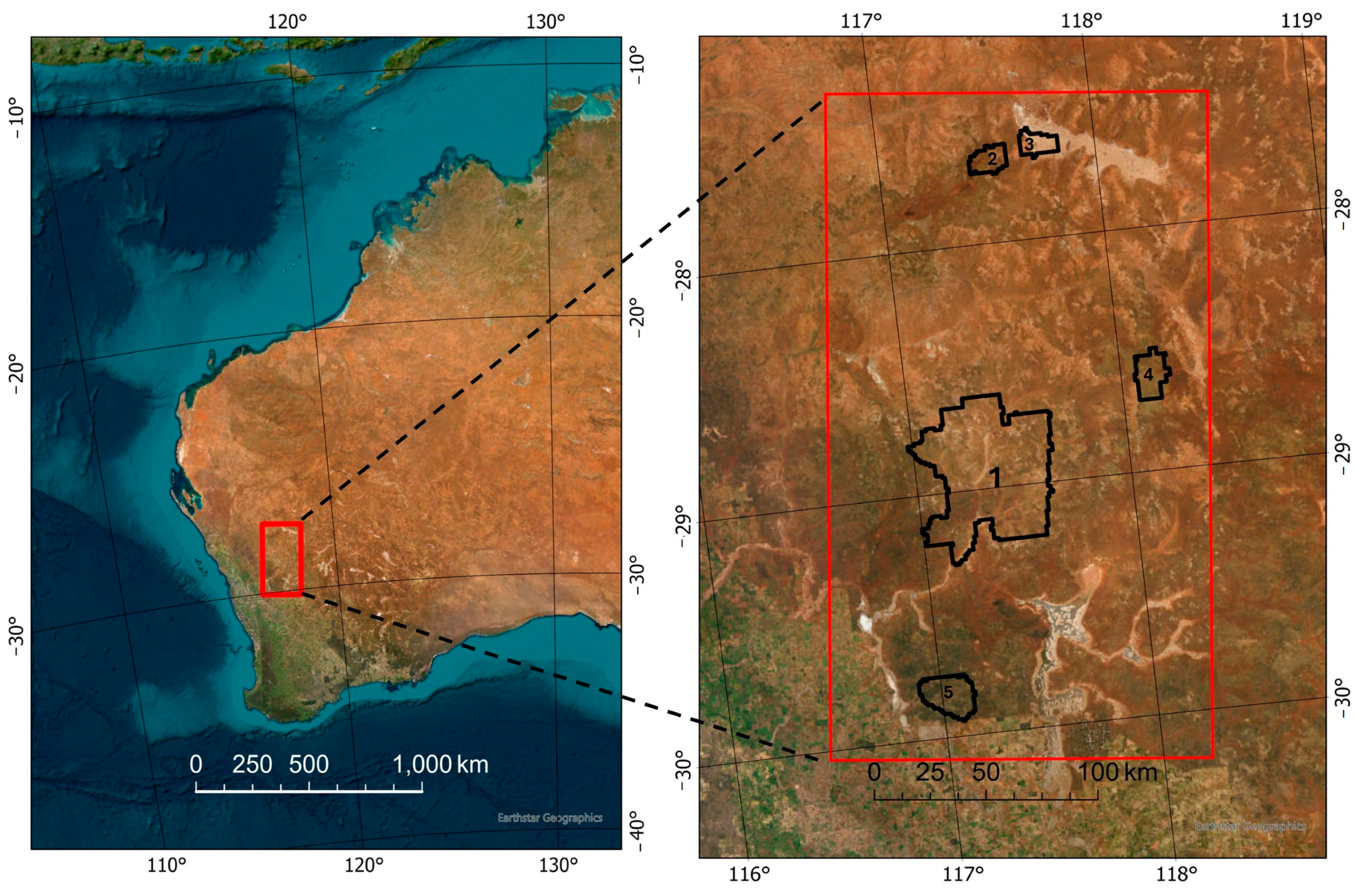
Data used for this study were collected in May 2021 over five different land blocks totalling 370,000 ha located in the Midwest region of Western Australia (Figure 1). The climate in this region is typically arid to semi-arid, with annual rainfall spanning between 200 and 250 mm and mean maximum and minimum temperatures of 30 and 12 °C [26]. All areas included in the study are currently managed by the Western Australian government for conservation purposes and predominantly support Acacia aneura sens. lat. (mulga) [27] woodlands and shrublands (hereafter mulga rangelands), as well as a range of other vegetation types (including eucalypt woodlands and chenopod shrublands).
Figure 1.
Extent of the aerial LiDAR data used for this study in the Midwest region of Western Australia, including 1: Thundelarra/Burnerbinmah Conservation Parks, 2: Lakeside National Park, 3: Lakeside Conservation Park, 4: Gagarlagu Nature Reserve, and 5: Bilunyi Wells Nature Reserve. (Background image credit: ESRI—Maxar, 2023).
2.2. LiDAR Data
ALS data were acquired using a Riegl VQ-1560i sensor flown at 1000 m above ground and processed by Fugro Australia Land Pty Ltd. (Perth, Australia). The point density commonly ranged between 15 and 20 points per square meter, with absolute scan angles below 30 degrees, and horizontal and vertical accuracies of 0.2 m and 0.1–0.15 m. The data points were obtained as ground/non-ground from the provider and were further processed using LAStools (v2.0.3) [28] to derive a series of vegetation structural metrics. The point cloud was filtered to remove noise and duplicate points, normalised to height above ground level, and then used to generate a canopy height model (CHM, by selecting the highest point in each 1 m2 using the lasgrid64 tool) at 1 m resolution. Outliers were removed by excluding points below 0 m or above 30 m, and all points ≤ 0.1 m were reclassified to 0 m to account for the vertical accuracy threshold.
2.3. Vegetation Structural Metrics
Twenty vegetation structural metrics were derived at 100 m resolution from the 1 m CHM (Table 1). This resolution (1 ha pixel) was selected to capture meaningful vegetation patterns in rangelands, whilst minimising confounding by finer-scale vegetation heterogeneity associated with groving (i.e., small patches of trees separated by more open spaces of bare ground and/or low sparse vegetation [29]). Most of the metrics derived from the CHM have been identified as relevant to vegetation structural differentiation by studies in other environments [16,20,30,31], although a number were included specifically for rangeland vegetation characterisation. Height intervals were adapted from the Australian National Vegetation Information System (NVIS) [32] to reflect common height characteristics of the most ubiquitous species in the mulga rangelands of WA [33]: 0, 0.1–1 m, 1–2 m, 2–5 m, 5–10 m, 10–20 m, and 20+ m.
Table 1.
The vegetation structural metrics derived from the 1 m resolution canopy height model and calculated at 100 m resolution.
Once the 1 m CHM were aggregated to 100 m resolution rasters for each structural metric, very clear banding patterns appeared in six of the variables in Table 1 (zmedian, p25, p50, covtotal, cov0, and cov0.1–1), particularly in areas dominated by lower vegetation (<1 m). These patterns have been reported as common artefacts in LiDAR-derived products and are considered in the discussion. Therefore, subsequent analyses used only the 15 variables without banding artifacts.
2.4. Unsupervised Classification
An unsupervised classification approach was used to delineate vegetation structural types using a fuzzy c-means clustering algorithm [23], implemented in the geocmeans package [34] in R 4.3.1 [35]. Unsupervised clustering is an exploratory technique that identifies intrinsic groupings within multivariate data without requiring predefined class labels. This approach was considered appropriate given the objective of identifying emergent vegetation structural types directly from the data, rather than assigning pixels to a priori defined classes.
While k-means clustering is commonly used in vegetation structural mapping [20,21,22], the fuzzy c-means approach provides additional advantages by allowing partial membership of each pixel across multiple classes. Specifically, each pixel is assigned a membership value (ranging from 0 to 1) for every class, with values summing to one. This enables explicit quantification of classification uncertainty and better represents gradual transitions in vegetation structure, which are characteristic of rangeland ecosystems.
All input variables were standardised between 0 and 1 [36], and correlation analysis was used to remove highly correlated variables (r2 > 0.7), resulting in a set of seven minimally redundant structural metrics (max, kurt, cov1–2, cov2–5, cov5–10, cov10–20, and cov20+).
The optimal number of clusters was identified using two complementary methods. First, “elbow plots” of the within-class sum of squares were inspected to identify points of diminishing improvement. Second, we applied a modified version of [20], repeatedly performing a two-step clustering procedure on a 10% stratified random sample of all 1 ha cells, using the Western Australian land system classification [37,38] as the stratification factor to improve representativeness. R packages bigmemory and biganalytics were used in this process [39]. This sampling approach reduced computational load from the full dataset (~370,000 samples) and accounted for potential inaccuracies in land system boundaries. Dendrograms and elbow plots were visually interpreted to select the final number of classes. After conducting unsupervised classification through the geocmeans package, each 1 ha pixel was assigned to its highest-membership class.
Class separability was assessed using a multi-step statistical procedure. A Kruskal–Wallis test evaluated overall differences among classes for each variable, followed by Dunn’s post hoc comparisons (dunn.test [40]). A rank-based MANOVA (manova.rm [41]) tested multivariate separability across all variables [20]. A linear discriminant function (LDF) analysis applied to a held-out 10% test subset produced a confusion matrix to identify well-separated and ambiguous class pairs and evaluate variable importance.
To characterise vegetation height profiles, 1000 randomly sampled 1 ha plots with membership certainty ≥ 0.9 were analysed. For each plot, the proportions of CHM pixels in height intervals (0, 0.1–1 m, 1–2 m, 2–5 m, 5–10 m, 10–20 m, and 20+ m) were calculated to produce average height-interval histograms for each class. Membership–certainty distributions for all mapped pixels were extracted to evaluate spatial confidence.
Further validation involved visual inspection of 50 randomly selected 1 ha polygons using contemporaneous 10 cm imagery. Height-profile histograms were generated for each polygon, and final class descriptions were defined using NVIS-based terminology for growth form, height, and cover [42,43,44,45].
Inspection identified a mixed “tall woodland” class, combining distinct eucalypt and tall mulga woodlands. A second fuzzy c-means classification was applied to these pixels using all Table 1 variables (since banding artefacts were absent in these areas), producing refined subclasses that replaced the original grouping. Finally, water bodies were removed using the Digital Earth Australia Waterbodies 3.0 dataset [46].
2.5. Validation
Given the remoteness and large spatial extent of the study area, the development of a comprehensive and spatially representative field validation dataset was not feasible. To address this limitation and strengthen the robustness of the analysis, two complementary validation approaches were implemented.
First, validation was conducted using field data collected in October 2021, approximately five months after the LiDAR acquisition. Vegetation height distributions were derived from systematic transect sampling in 14 plots (50 m × 50 m) within Thundelarra Conservation Park (Figure 1). In each plot, four north–south and four east–west transects were established, and vegetation height was recorded at 1 m intervals. Measurements were aggregated into the same height classes used in the unsupervised classification and expressed as proportions of sampled points, providing an estimate of percentage cover for each height class.
These observed distributions were compared with reference height profiles (mean values per height bin) derived from 1 ha pixels assigned to structural classes with high classification confidence. For each plot, the absolute differences between observed and reference percentage cover were calculated across all height bins and summed to quantify dissimilarity for each structural class. The classes with the lowest and second-lowest summed differences were identified as the best and second-best matches, respectively. All plots were located within areas mapped as structurally homogeneous at the 1 ha resolution.
Second, an independent sample-based validation was conducted to further assess classification performance under limited field accessibility. A stratified random sample of fifty 1 ha plots per structural class was selected. For each plot, 10 cm resolution RGB imagery acquired concurrently with the LiDAR survey was visually interpreted alongside LiDAR-derived height distribution histograms. Based on this combined information, each plot was independently assigned to a structural class. These independent assignments were compared with the LiDAR-derived classification to produce a confusion matrix, from which class-balanced accuracies, overall accuracy, and Cohen’s kappa coefficient were calculated.
2.6. Spatial Clustering of Membership Certainty
To evaluate if spatially clustered areas of high and low membership certainty were found within particular areas or in specific vegetation structural classes, we applied a Getis-Ord Gi analysis [47] to a final membership certainty raster layer generated by assigning each pixel with the highest membership value of the c-means classification. The Getis-Ord Gi statistic identifies localized clusters (hotspots and cold spots), highlighting where significantly high or low values occur together in space. This analysis was conducted in ArcGIS Pro 3.1.0 (Redlands, CA, USA).
2.7. Comparison with Previously Existing Vegetation Mapping and Condition Products
Finally, to put our results in the context of current Australian vegetation mapping and condition products, we overlaid our vegetation structural types map with the NVIS Major Vegetation Subgroups [32], as well as with the latest Habitat Condition Assessment System evaluation [48]. These comparisons are presented in the Supplementary Materials and help us guide part of the discussion.
3. Results
3.1. Vegetation Structural Types Separation and Definition
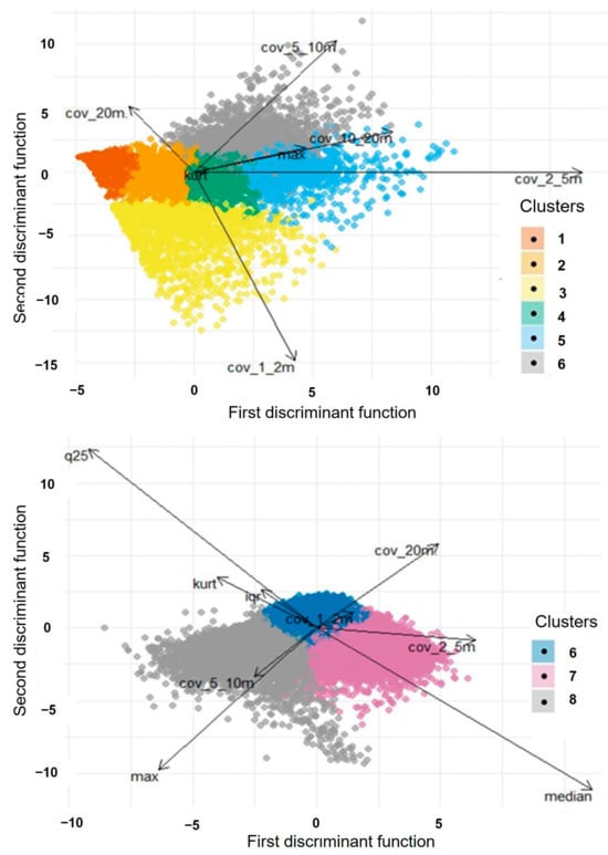
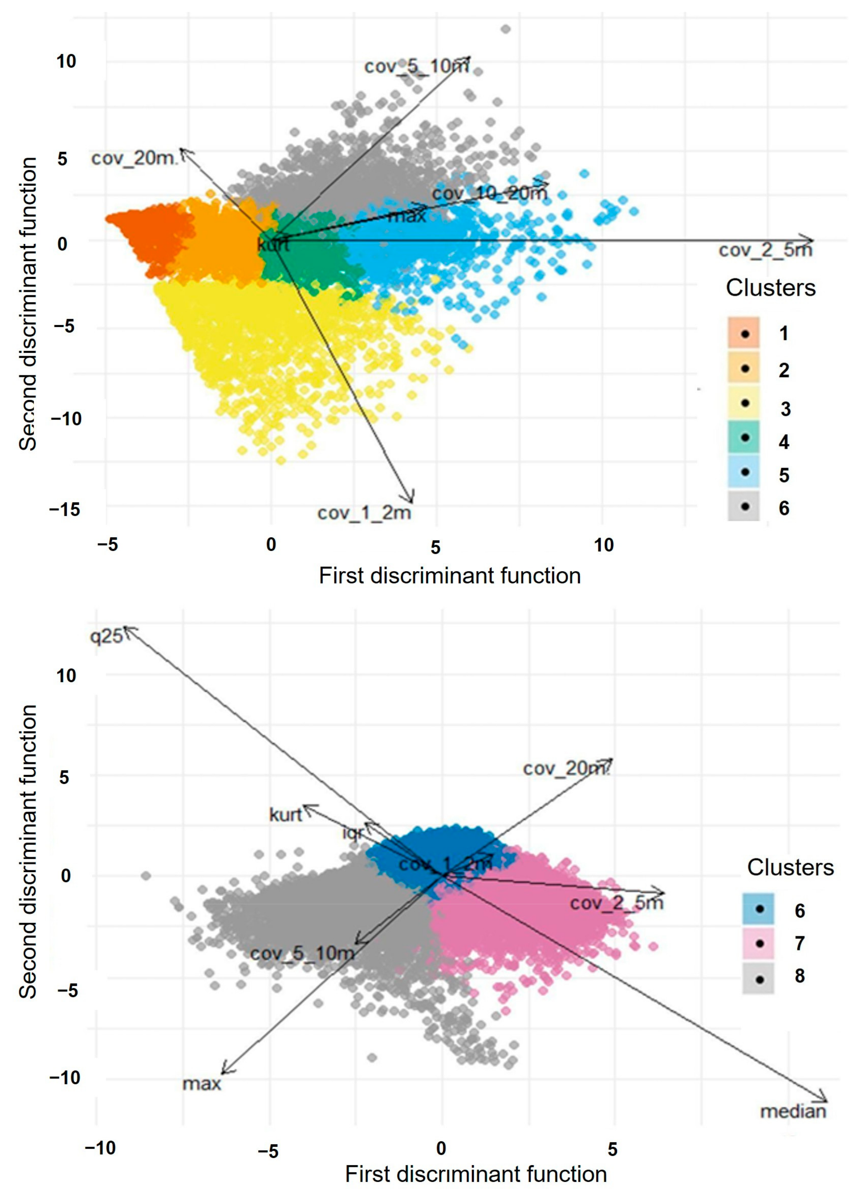
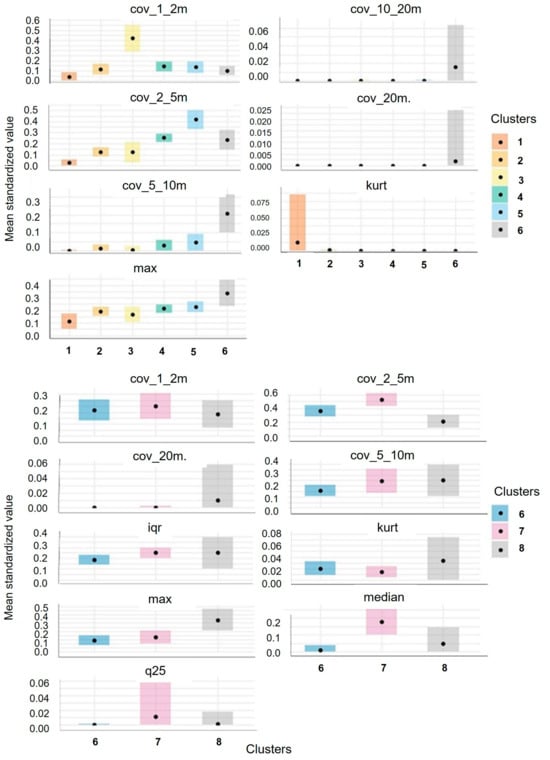
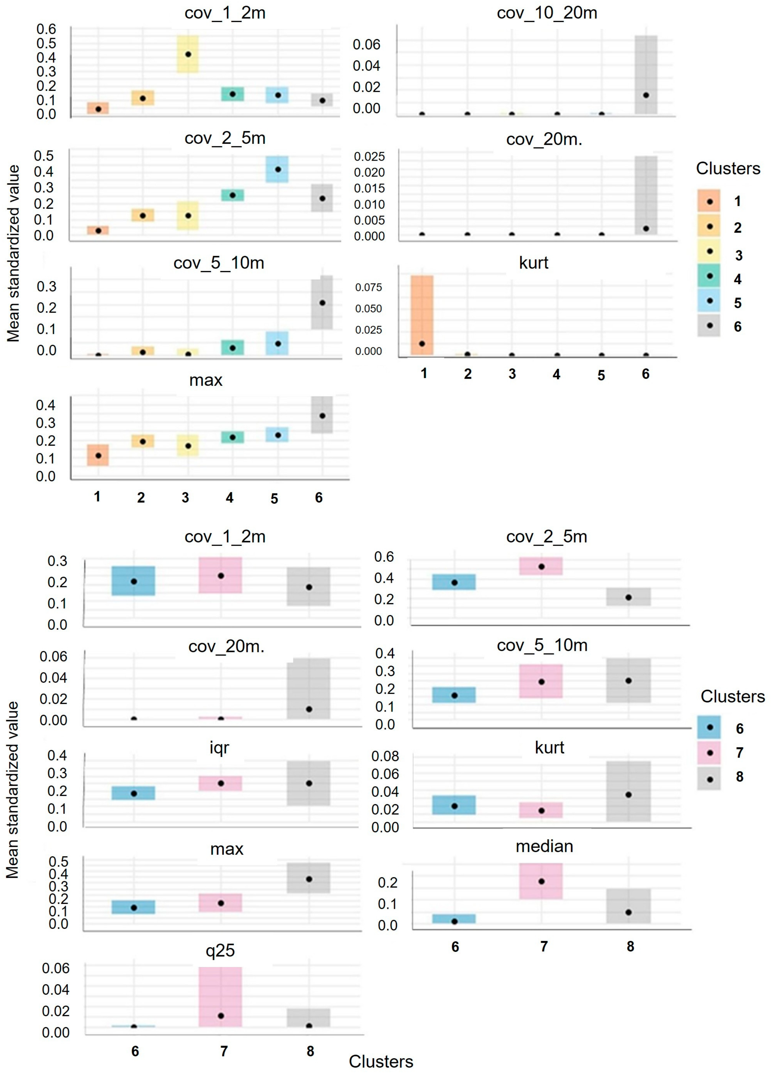
The optimal number of classes for the unsupervised classification was assessed using the elbow method, based on the relationship between the number of classes (k) and the within-cluster sum of squares (WCSS). The resulting curve showed a reduction in WCSS up to k = 5, after which the rate of decrease diminished substantially, with only marginal gains observed beyond k = 6 (Figure S1). This inflection point—interpreted as the “elbow”—occurred between k = 5 and k = 6, suggesting that the optimal number of clusters lies within this range. The 100 dendrograms produced in the two-step clustering procedure on a 10% stratified random sample of all 1 ha cells pointed towards a six-class system as the most representative of the data (Figure S1). Consequently, we proceeded with a fuzzy c-means unsupervised classification with six classes set as the number of clusters to be generated by the algorithm. The Kruskal–Wallis test and rank-based MANOVA showed significant differences among classes for every variable (p < 0.001), and Dunn’s post hoc test found all pairwise comparisons significant (p < 0.001). Linear discriminant function (LDF) analysis achieved 91.5% accuracy with the held-out test dataset (Table S1), and classes were clearly separated along the first two discriminant functions (Figure 2), which explained 80.9% of total variance (62.4% and 18.5%). Cover between 1–2 m, 2–5 m, 5–10 m, and maximum height were the most influential variables in separating structural classes (Figure 2 and Figure 3).
Figure 2.
(Top panel): The linear discriminant function outputs, where 10% of all samples are assigned into clusters (which were subsequently labelled as different vegetation structural classes) through an unsupervised classification, and plotted against their value in the first two discriminant functions. (Bottom panel): The linear discriminant function outputs, where all samples within the initial “tall woodlands” cluster (cluster 6 in the (top panel)) were assigned into one of three sub-clusters through an unsupervised classification, and plotted against their value in the first two discriminant functions. The arrows’ lengths and directions indicate the relative contribution of each structural metric to cluster separation. Abbreviations—max: maximum height; kurt: kurtosis; median: median height; iqr: inter-quartile range of height; q25: 25th percentile of height; cov_1_2m: cover between 1 and 2 m; cov_2_5m: cover between 2 and 5 m; cov_5_10m: cover between 5 and 10 m; cov_10_20m: cover between 10 and 20 m; and cov_20m.: cover above 20 m.
Figure 3.
(Top panel): The mean standardized values of the identified six clusters (which were subsequently labelled as different vegetation structural groups) for each lidar-derived variable used in the first unsupervised classification. (Bottom panel): The mean standardized values of the identified three clusters (which were subsequently labelled as different vegetation structural classes) identified within the initial “tall woodlands” (class 6 in the (top panel)) for each lidar-derived variable used in the unsupervised classification. Boxplots represent the mean as a black dot ±1 standard deviation as the top and bottom edges of each box, with negative values not plotted. Abbreviations—max: maximum height; kurt: kurtosis; median: median height; iqr: inter-quartile range of height; q25: 25th percentile of height; cov_1_2m: cover between 1 and 2 m; cov_2_5m: cover between 2 and 5 m; cov_5_10m: cover between 5 and 10 m; cov_10_20m: cover between 10 and 20 m; and cov_20m.: cover above 20 m.
Within the six structural classes, the “tall woodlands” class was subdivided into three statistically separable sub-classes. The sub-division of the class defined as “tall woodlands” showed an elbow plot and clustering patterns where at least three classes could be statistically separated (Figure S2). We decided against defining more than three classes to keep the classification system simpler and in accordance with what is known of these tall woodland areas in the southern rangelands of WA. Although more than three clusters were optimal, only three were retained for ecological interpretability. Kruskal–Wallis, MANOVA, and Dunn’s test all showed significant differences (p < 0.001). Linear discriminant analysis achieved 96.5% accuracy (Table S2), with the first two discriminant functions explaining 99.2% of variance (63.2% and 36.8%). Median height, maximum height, and the 25th percentile height were the most influential variables when subdividing this “tall woodland” class (Figure 2 and Figure 3).
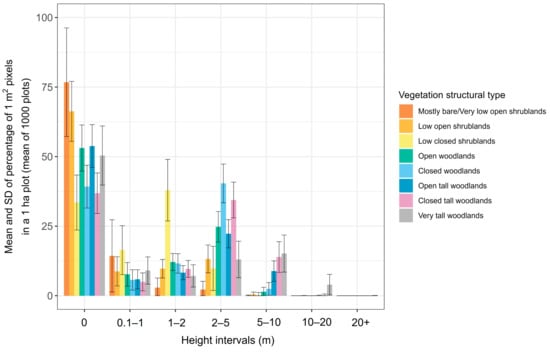
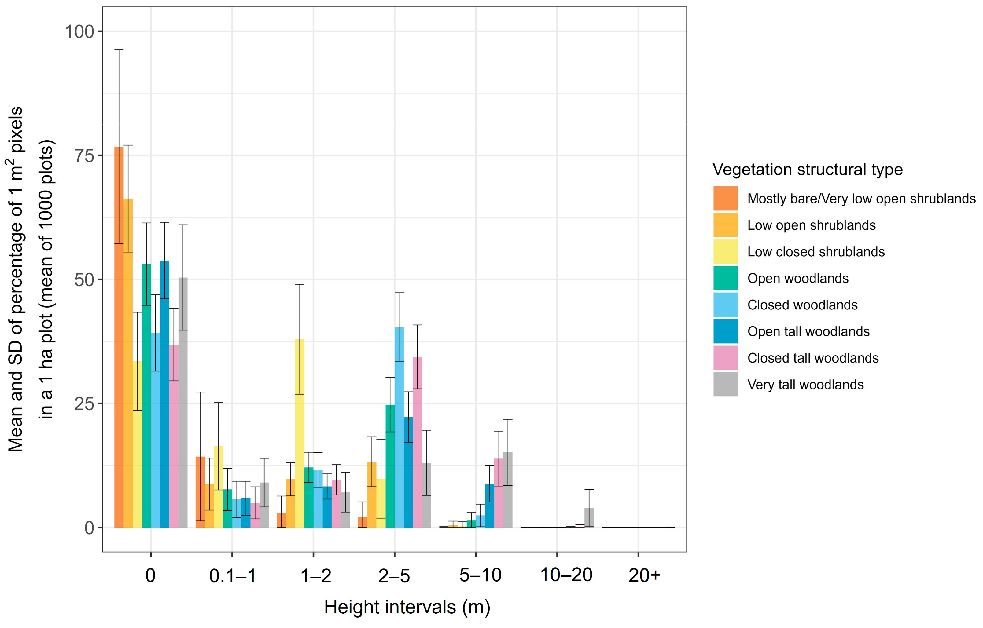
The height-interval histograms for the eight final structural classes showed typical vegetation height distributions across 1000 randomly selected 1 ha pixels with membership certainty ≥ 0.9 (Figure 4). These histograms, together with visual inspection of 50 randomly selected 1 ha plots per class using 10 cm imagery, informed the extended class definitions in Table 2, which also lists the corresponding NVIS structural classes [32]. The proportions of NVIS Major Vegetation Subgroups within each structural class are shown in Table S3 and Figure S4. To provide a broader comparison, we calculated the percentage of the study area covered by our structural types and by NVIS subgroups (Table S4). Overall, our study area was dominated by “Mulga (Acacia aneura) woodlands and shrublands +/− tussock grass +/− forbs” and “Other Acacia tall open shrublands and shrublands”. High bare-ground representation reflects the naturally open rangeland vegetation.
Figure 4.
The mean and standard deviation in the % proportion of 1 m2 pixels in different height intervals in the 1000 one-hectare plots that were classified with a membership certainty of 0.9 or higher for each one of the final vegetation structural classes.
Table 2.
Definitions of the eigth vegetation structural classes as a result of the first and second unsupervised classifications using LiDAR-derived structural metrics, and the approximate match with the National Vegetation Inventory System (NVIS) putative structural classes [32]. Note that classes shown with an asterisk (*) were derived from class number 6 in this table.
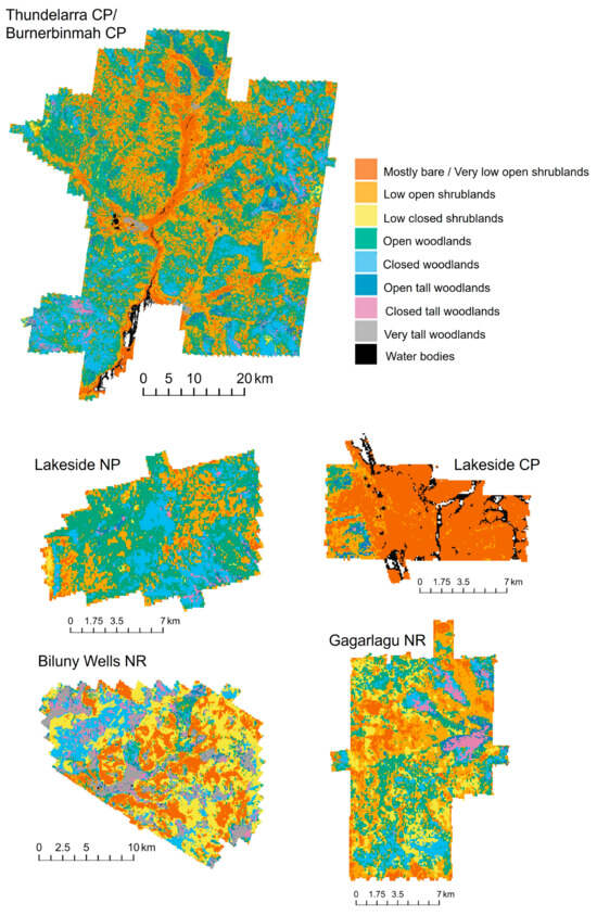
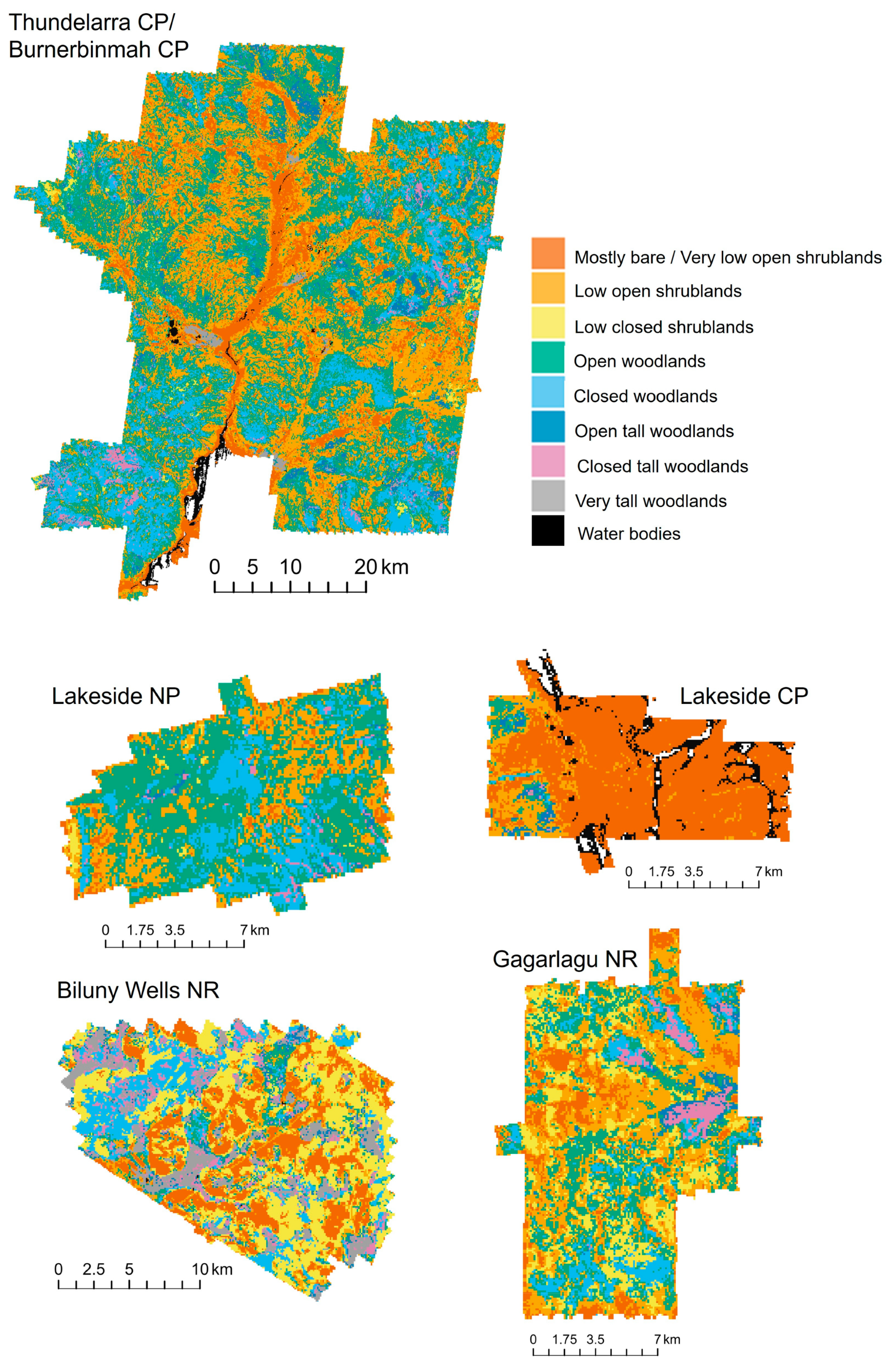
Adding the water body mask, we created a final vegetation structural class map for the ALS-surveyed areas (Figure 5). We also show a graphic example of each vegetation structural type, including a snapshot of a typical high-resolution image, a picture of that same imaged plot from the ground, and a transect of the LiDAR point cloud in the same area showing typical vegetation distribution in height for each class (Figure S7).
Figure 5.
Map of vegetation structural classes resulting from two sequential unsupervised classifications performed in this study in five land blocks in the mulga rangelands of Western Australia over which aerial LiDAR data was collected in May 2021. Abbreviations—NP: national park, NR: national reserve, CP: conservation park.
3.2. Validation Through Field Plots and High-Resolution Imagery with Height Profiles
The comparison between field-derived height profiles and the results of the unsupervised classification is summarised in Table 3. Although not all structural classes were represented in the field dataset (with no samples corresponding to “low closed shrublands”, “closed woodlands”, and “tall closed woodlands”), 12 out of 14 plots exhibited height distributions that corresponded to either the first or second best-matching structural class based on the reference height profiles shown in Figure 4.
Table 3.
Comparison between the height profiles in the 14 field plots in the Thundelarra Conservation Park and the results of the unsupervised classification. The class numbers correspond to: 1—mostly bare/very low open shrublands, 2—low open shrublands, 3—low closed shrublands, 4—open woodlands, 5—closed woodlands, 6—tall open woodlands, 7—tall closed woodlands, and 8—very tall woodlands.
For each plot, the summed absolute differences in percentage cover across all height bins are reported for both the best and second-best matches, providing a quantitative measure of similarity between the observed field plot height profiles and reference profiles. The classes “mostly bare/very low open shrublands” and “low open shrublands” were the most frequently represented in the validation dataset, consistent with their dominance across the study area.
Two plots located in areas classified as “open woodlands” in the unsupervised classification did not show height profiles that matched the expected height distribution. Instead, their field-measured height profiles were more similar to those of “low open shrublands” and “tall open woodlands”. The histograms showing how the field plot height profiles, compared with the two closest vegetation structural class height profiles (as shown in Figure 4), are included in Figure S8.
The validation process we conducted, based on high-resolution imagery and height profiles for 50—1 ha plots for each vegetation structural type, resulted in a confusion matrix presented in Table 4. Balanced class accuracies ranged between 82 and 96%, with a kappa coefficient of 0.77 and an overall accuracy of 79.5%. The classes “mostly bare/very low open shrublands”, “low closed shrublands”, “tall open woodlands”, and “very tall woodlands” showed the highest balanced class accuracies, over 90%. “Low open shrublands” and “closed woodlands” showed the lowest values, in the low 80’s.
Table 4.
Confusion matrix and classification accuracy parameters according to a visual evaluation of high-resolution (10 cm) imagery of 50—1 ha plots per vegetation structural class. Class numbers correspond to: 1—mostly bare/very low open shrublands, 2—low open shrublands, 3—low closed shrublands, 4—open woodlands, 5—closed woodlands, 6—tall open woodlands, 7—tall closed woodlands, and 8—very tall woodlands.
3.3. Membership Certainty
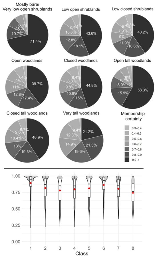
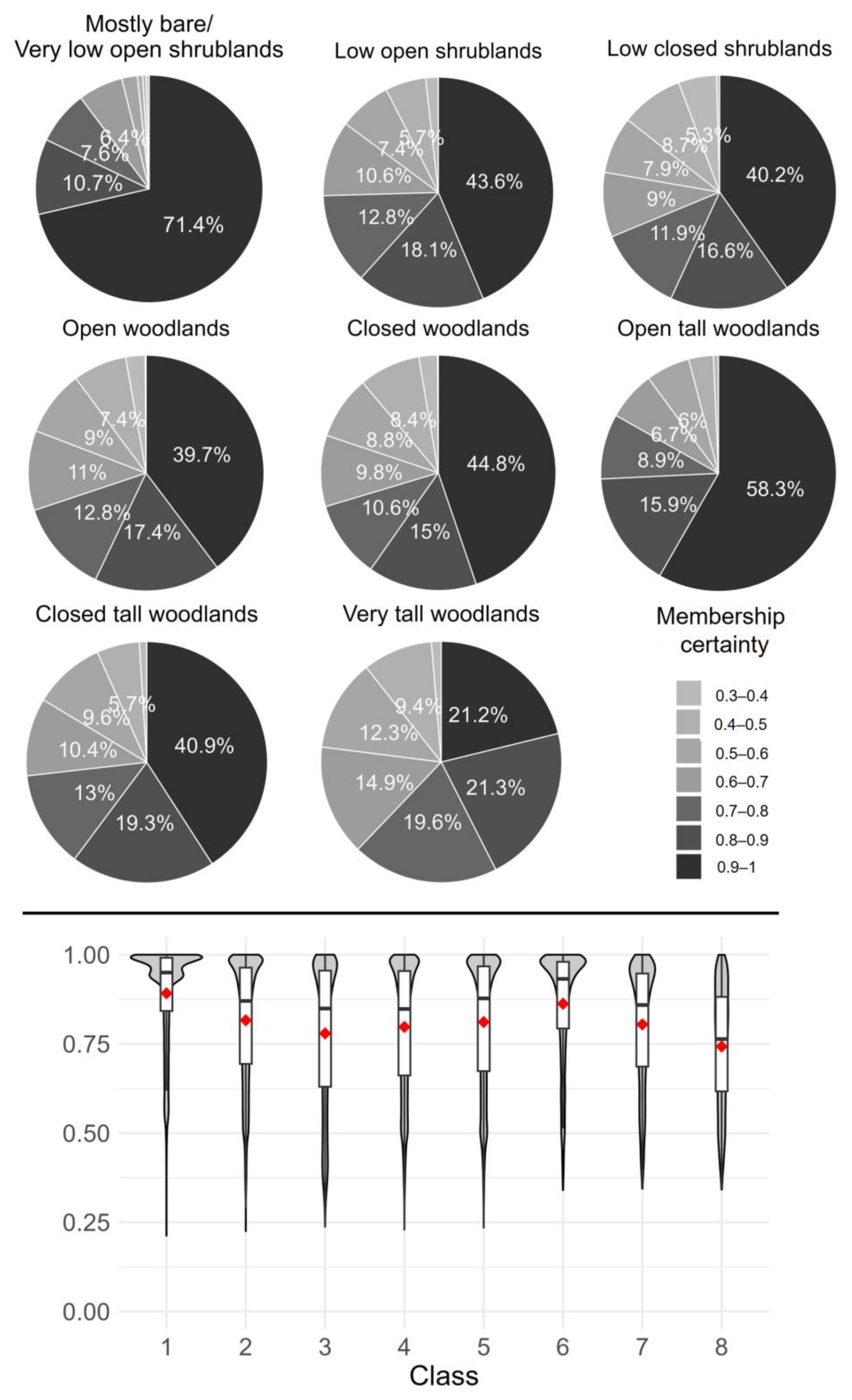
Membership certainty of the final classification map showed that 74.5% of the study area achieved a certainty of ≥0.7, and 46.5% was mapped with very high certainty (≥0.9) (Figure 6). All five blocks had at least 50% of their area mapped with certainty ≥0.7. Lakeside CP had the highest certainty (74.9% ≥0.9), while Gagarlagu NR had the lowest (54.5% ≥0.7) (Figure S3).
Figure 6.
(Top panel): Pie charts showing the distribution of membership certainty for each one of the vegetation structural classes resulting from the two unsupervised classifications performed in this study. (Bottom panel): The distribution of the fuzzy membership certainty (range 0–1) for each of the eight classes derived from the unsupervised classification. For each class (1–8), the violin plots represent the full distribution of pixel-level membership values, with width proportional to the density of observations. The overlaid boxplots summarize the central tendency and dispersion, where the central line indicates the median, the box bounds the interquartile range (IQR; 25th–75th percentiles), and the whiskers extend to the most extreme values within 1.5 × IQR. The red diamond symbols denote the mean membership value for each class. The class numbers correspond to: 1—mostly bare/very low open shrublands, 2—low open shrublands, 3—low closed shrublands, 4—open woodlands, 5—closed woodlands, 6—tall open woodlands, 7—tall closed woodlands, and 8—very tall woodlands.
The two dominant vegetation structural classes were “low open shrublands” and “open woodlands” (30.3% and 30.0% of the study area). Both feature extensive open ground with low (<2 m) and tall (>5 m) vegetation (Figure 4 and Figure 7), but “open woodlands” contain more vegetation between 2 and 5 m. These two classes also contained contiguous areas of low membership certainty due to structural similarity and high representation (Figure S3), making them difficult to distinguish visually in 10 cm imagery. However, their statistical separability (Table S1) and relatively high proportions of high-certainty pixels (Figure 6) confirm they represent distinct structural classes.
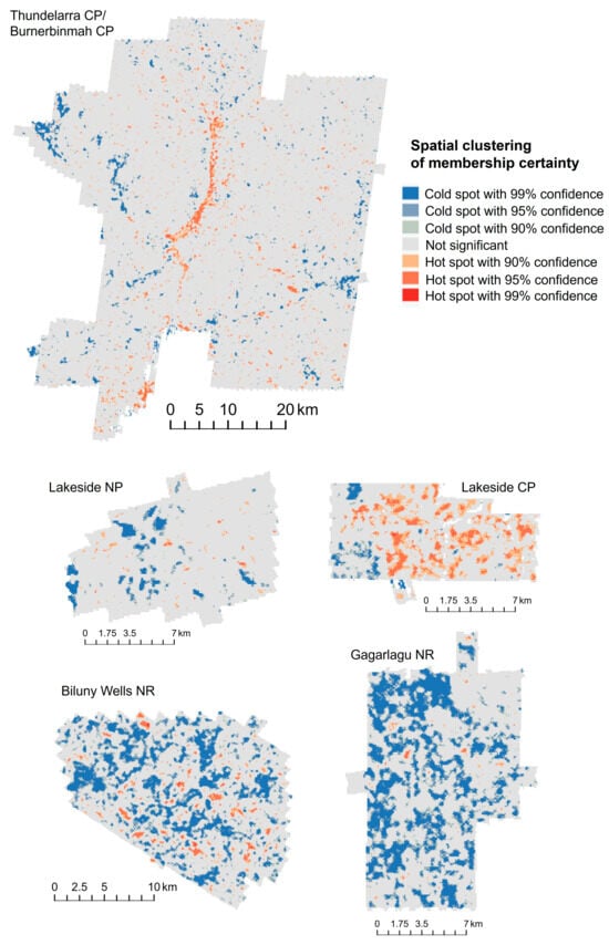
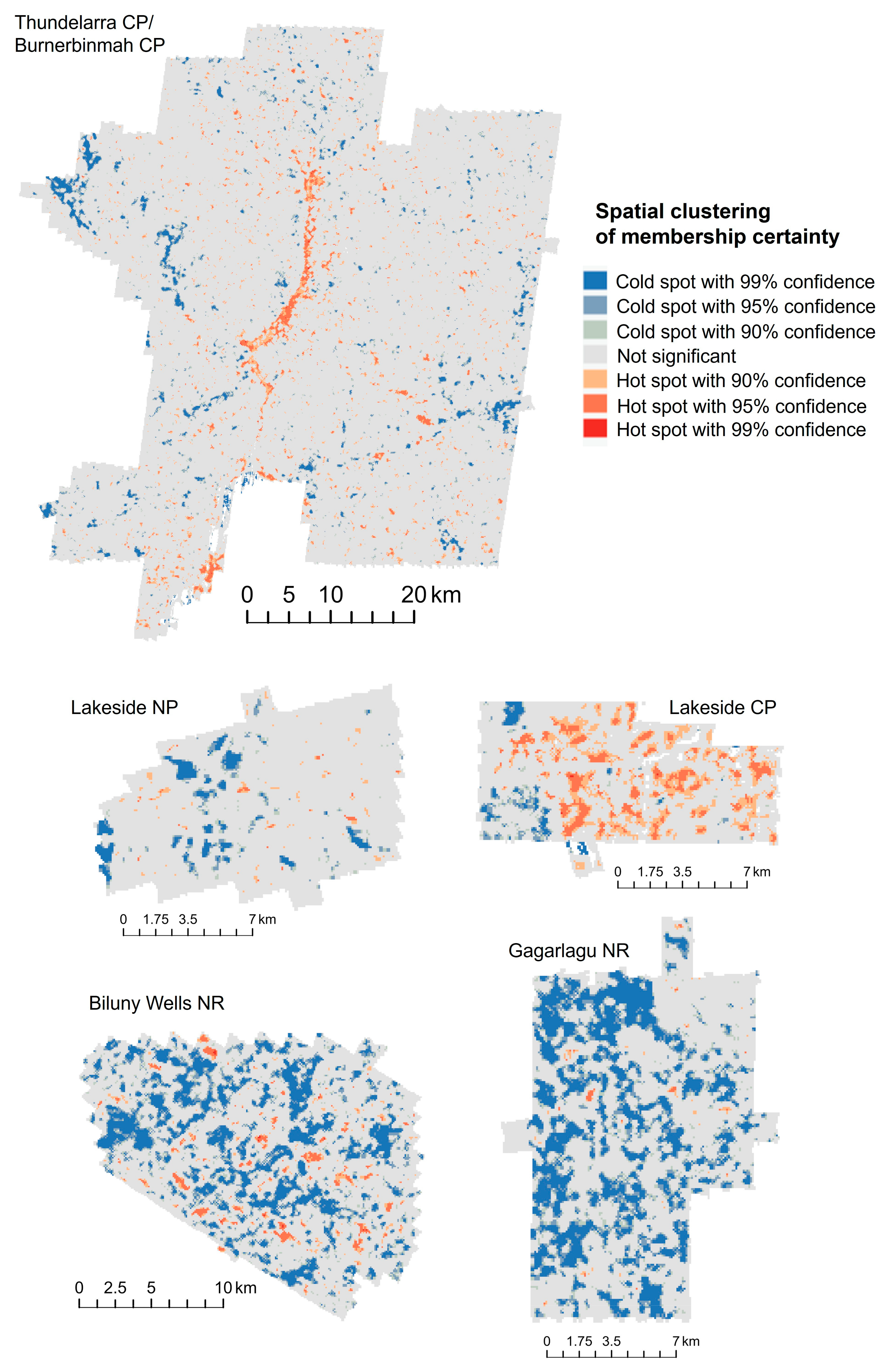
Figure 7.
The spatial distribution of membership certainty clustering in five land blocks in the mulga rangelands of Western Australia. Areas identified as cold spots indicate significant spatial clustering of 1 ha pixels with lower membership certainty as a result of the fuzzy c-means classification. Areas identified as hot spots indicate significant spatial clustering of 1 ha pixels with higher membership certainty resulting from the fuzzy c-means classification.
“Closed woodlands” covered 13.6% of the landscape and were classified with high certainty (>70% mapped with ≥0.7, and mean and median certainties of 0.89 and 0.95, respectively). They are characterised by vegetation between 2 and 5 m, reaching up to 40% cover within a 1 ha pixel (Figure 3 and Figure 4).
Areas dominated by bare ground (typically ~75%, sometimes >90%) and/or very low vegetation (<1 m) comprised 13.3% of the study area. Found mainly in drainage lines and flood-prone areas, they also occurred within other classes (especially within “low open shrublands,” “open woodlands,” and “low closed woodlands”). Although not always spatially contiguous, this class was easily separable, with >70% of pixels showing very high certainty (≥0.9) and mean and median certainties of 0.82 and 0.87, respectively (Figure 6).
“Low closed shrublands” formed a structurally unique class dominated by 1–2 m vegetation with up to 50% cover. It was mostly restricted to Biluny Wells NR, appearing with lower accuracy in Gagarlagu NR and occasionally within “low open shrublands” and “open woodlands”, and showed relatively high membership certainty values (mean and median certainties of 0.78 and 0.85, respectively).
The three tall woodland sub-classes showed clear differentiation. “Closed tall woodlands” had larger median and 25th-percentile heights and contained mainly vegetation between 2 and 5 m, distinguishing them from “very tall woodlands,” which had the largest proportions of trees >10 m, with some >20 m. “Closed tall woodlands” represent a denser version of “open tall woodlands,” which had the second-highest proportion of high-certainty area (almost 60% ≥0.9, and mean and median certainties of 0.86 and 0.93, respectively) (Figure 6).
3.4. Spatial Patterns of Membership Certainty
The spatial patterning of membership certainty varied across vegetation structural classes (Figure 7 and Figure S3). “Low closed shrublands” and “very tall woodlands” had the highest proportion of cold spots, whereas “mostly bare/very low open shrublands” showed the highest proportion of hot spots (Figure S3). Biluny Wells NR and Gagarlagu NR contained the most cold spots, particularly within “low open shrublands,” “low closed shrublands,” and “open woodlands.” Nearly one-third of Lakeside CP showed hot spots in the “mostly bare/very low open shrublands” class. Spatial clustering patterns differed among land blocks, with high-confidence mapping in Thundelarra/Burnerbinmah CP and Lakeside CP, and low-confidence clusters in Biluny Wells NR and Gagarlagu NR.
3.5. Overlay with Current Ecological Condition Assessment
Finally, when we overlaid the 2020–2022 HCAS assessment for our study area, we found that most of it was attributed with a high condition score (close to 1) (Figure S5). Overall, the “mostly bare/very low open shrublands” structural class showed the lowest condition values, particularly in Lakeside NP and CP, and in the Thundelarra/Burnerbinmah CP. (Figure S6). In this latter land block, “very tall woodlands” also showed lower condition values compared to other structural classes.
4. Discussion
We used high-density ALS data to identify and map eight statistically distinct vegetation structural classes across 370,000 ha of semi-arid rangelands. We were able to relate these types to structural descriptors that broadly resemble existing field-based structural classifications, and we attributed each vegetation structural class and each 1 ha pixel within our study area with measures of mapping confidence. This structural characterisation highlights a novel use of ALS data in rangelands, providing a baseline upon which ecological conditions can be assessed in landscapes where degradation is widespread but poorly understood spatially, and where existing information on the spatial distribution of vegetation structural types is lacking.
4.1. Comparison with Previous Approaches
Our data-driven identification of vegetation structural classes differs fundamentally from previous rangeland studies that relied on predefined categories and lower-density airborne laser scanning (ALS) data. For example, Ref. [17] worked in temperate and wet rangelands using ALS point densities of 0.25–1.5 points m−2 and attempted to map three predetermined vegetation types; however, they were able to reliably distinguish only two, failing to separate shrubland from grassland. Similarly, Ref. [18] combined 1 point m−2 LiDAR with satellite imagery to classify riparian vegetation types defined a priori based on ecological knowledge. In both cases, classification performance was constrained by the need to impose well-established structural descriptions of target vegetation types.
In contrast, our approach used height-interval metrics tailored to rangeland vegetation while avoiding assumptions about which structural types should be present. The substantially higher point density of our dataset (~15 points m−2) enabled detection of very sparse vegetation elements that are commonly missed in low-density surveys. When paired with an unsupervised framework—critical in a region with limited field data—this higher resolution allowed structural classes to emerge directly from the data rather than being forced into pre-existing schemes. This provides a more flexible, context-specific representation of vegetation structure in arid and semi-arid rangelands with long histories of ecological degradation.
Forest studies offer the closest methodological comparisons, as no equivalent rangeland analyses exist using high-density ALS. Ref. [20], working with 1–4 points m−2 ALS data, used similar methods to delineate structural divisions in forest environments. As in our study, proportional vegetation cover within height intervals explained most variation, reinforcing the relevance of these metrics beyond forested settings and supporting their applicability in rangelands. We extended the internal separability evaluation framework presented in [20] by incorporating a two-fold independent validation approach based on (i) field measurements, and (ii) visual interpretation of high-resolution RGB imagery. Importantly, we have now included a field-based validation component derived from in situ vegetation measurements. Although this dataset is limited in the number of plots, as well as in its spatial representativeness and distribution across the study area, it provides an independent and ecologically grounded reference for evaluating the classification outcomes.
As the classification was derived using an unsupervised approach, no externally defined “ground truth” classes are available. Instead, the validation procedure assesses: (i) whether vegetation height profiles measured in the field correspond to the characteristic height distributions of the structural classes identified through clustering, and (ii) whether the resulting clusters represent ecologically meaningful and visually interpretable vegetation structural patterns. Thus, the evaluation is not based on independent categorical labels, but rather on the consistency between mapped classes and observable structural attributes (e.g., canopy height, cover, and vertical complexity) derived from field observations, LiDAR data, and high-resolution imagery.
While this approach does not constitute a rigorous, statistically representative field-based accuracy assessment, it provides a structured and independent evaluation of the ecological plausibility of the classification. The inclusion of field data, albeit limited in extent, strengthens confidence in the correspondence between LiDAR-derived structural metrics and on-ground vegetation characteristics. The complementary use of high-resolution imagery and LiDAR-derived height profiles further enables the assessment of both horizontal and vertical vegetation structure, which is particularly important in rangeland systems where vegetation gradients are continuous rather than discrete.
Overall, this validation framework is consistent with exploratory clustering approaches, where the primary objective is to identify meaningful patterns in the data rather than to reproduce predefined classes. More importantly, the agreement between field-derived and LiDAR-based height profiles, as well as the validation step based on visual interpretation of high-resolution imagery, supports the capacity of the unsupervised classification to capture ecologically meaningful variation in vegetation structure.
Our use of fuzzy c-means clustering provided additional information by quantifying classification confidence for every pixel. This is particularly valuable in rangeland environments where vegetation boundaries are often subtle, and species with contrasting structural attributes co-occur. By allowing partial membership across classes, the method explicitly captures ambiguity in transitional zones and mixed patches. Mapping this uncertainty highlights areas where structural assignments are less reliable and where additional field validation or flexible management responses may be required. Such information strengthens the interpretability of structural maps for restoration planning and ecological assessment in degraded rangelands.
4.2. Technical Limitations and Solutions
Banding artefacts in aerial LiDAR data, as observed in our study, can be caused by increased point intensity in swath overlap areas and are a known issue that can distort vegetation structural metrics [49,50]. In our study, mostly bare areas and areas dominated by very low open shrublands were mostly affected by these artefacts, which were particularly evident in the structural metrics influenced by dominant lower vegetation attributes (zmedian, p25, p50, covtotal, cov0, and cov0.1–1). While removing overlap points can eliminate banding, it introduces abrupt changes in point density between swaths [51], which also affects data quality. Attempts to homogenize point density using thinning and voxelization methods did not fully resolve the issue in our case, as banding persisted in structural metrics after resampling to 1 ha pixels. Working with a canopy height model helped reduce these artifacts, but banding remained in some variables after resampling. We hypothesise that increased point density in overlap areas likely enhanced the detection of smaller vegetation components, leading to artificial patterns in swath overlap areas dominated by low open vegetation, common in rangelands. In contrast, taller vegetation (>1 m) was unaffected due to its larger structure, which is consistently detectable across varying point densities.
The inability to distinguish further classes within the first meter of vegetation has important management implications, as chenopod shrublands—key forage species and indicators of ecological health—may be present. Future LiDAR-based rangeland studies should ensure larger overlaps between ALS swaths to achieve equal (and high) point density distribution across the landscape. This would allow for a homogenised detection probability of lower/smaller vegetation elements, eliminating banding artifacts and allowing to confidently use of data corresponding to the lowest vegetation strata.
4.3. Vegetation Structural Characterisation Framework
In Australia, vegetation structural characterisation has been approached through descriptions and studies that do not provide sufficient information to support rangeland management for biodiversity conservation and restoration across large extents, such as the mulga rangelands of Western Australia. The National Vegetation Information System (NVIS) provides an Australia-wide framework to classify native vegetation, incorporating structural characterisation adapted from [42,43,44,52]. Its broad-scale design requires coverage of structural variation across many ecosystem types, not solely rangelands. More recently, Ref. [53] adapted NVIS structural classes into a remote-sensing method for continental-scale vegetation structure mapping, and Ref. [18] further modified these classes for arid riparian environments.
In our study, we adapted structural classes to better reflect vegetation structure in mulga rangelands by measuring percentage cover across height intervals relevant to typically low, sparse rangeland vegetation, alongside commonly used metrics such as maximum height and kurtosis [16,30,31]. Our 1 ha pixel resolution also represents a deliberate departure from the 30 m resolution used in Landsat-based studies [18,53]. This coarser resolution incorporates characteristic bare-ground patches while capturing ecological and hydrological processes relevant at management scales.
4.4. Ecological Condition Assessments and Structural Mapping
Our vegetation structural mapping provides a way to strengthen rangeland condition assessments. Although the continental HCAS tool classifies most of the study area as being in good condition, land managers report that parts of the ex-pastoral stations remain substantially degraded, lacking palatable shrubs and perennial grasses. This aligns with the broader understanding that mulga rangelands formerly used for grazing often persist as modified states of the original ecosystem, containing mixtures of reference, altered, or collapsed components. Our structural map can therefore guide targeted field validation to refine condition assessments.
The map also shows greater structural diversity than existing NVIS units. NVIS mapping in this region relies on decades-old photo interpretation, whereas our ALS-derived classification captures finer-scale variability. Apparent discrepancies—such as chenopod shrublands within NVIS eucalypt woodland units—likely reflect scale mismatches. Some variation may also indicate condition differences within a single vegetation type. However, structure alone cannot separate condition-driven change from natural variation, highlighting the need to integrate structural data with soils, geology, climate, and terrain to support ecological condition assessments.
4.5. Future Directions
Large-scale vegetation structural assessment currently requires expensive ALS data acquisition. Developing methods to predict ALS-derived metrics from freely available satellite imagery (optical and radar) represents the next critical step for operational implementation. Machine learning approaches show promise for wall-to-wall structural mapping in Australia [53], but this must be tested with rangeland-specific structural types, which, as proven in this study, can be defined by several height intervals below 10 m. Integration of such wall-to-wall products with vegetation cover measures could help link structure to ecosystem processes, contributing to more comprehensive rangeland ecological condition assessments.
5. Conclusions
High-density ALS data successfully mapped vegetation structural heterogeneity in rangelands through unsupervised classification, providing potential baseline information for ecological management. Despite limitations characterising low vegetation strata, the classification significantly improved the understanding of vegetation structure distribution across areas typical of rangeland management units (such as ex-pastoral stations). Combined with vegetation cover dynamics and accurate environmental characterisation, the structural maps presented here could support management of rangeland ecosystems facing mounting pressures from climate change and historical overgrazing-derived erosion processes. Future research should address low vegetation characterisation through improved LiDAR data acquisition protocols and develop satellite-based approaches for cost-effective structural monitoring.
Supplementary Materials
The following supporting information can be downloaded at: https://www.mdpi.com/article/10.3390/rs18101641/s1, Figure S1: “Elbow plot” showing the change in within-class sum of squares against the number of classes (left panel), and typical dendrogram (most representative out of 100 stratified iterations) resulting of a two-step clustering method to identify the number of groups that maximized differences between them (right panel); Figure S2: “Elbow plot” showing the change in within-class sum of squares against the number of classes within “tall woodland” (cluster 6 of first unsupervised classification) (left panel), and a dendrogram resulting of a two-step clustering method to identify the number of “tall woodland” sub-classes that maximized differences between sub-classes (right panel); Figure S3: Membership certainty values of the final vegetation structural map (Full dataset) and for each one of the five land blocks covered by the Aerial LiDAR Scanning dataset (values closer to 1 signal stronger membership probability); and spatial clustering of membership certainty for each one of the vegetation structural classes in the final vegetation structural map within each one of the five land blocks (bar plots); Figure S4: Distribution of National Vegetation Inventory System (NVIS) Major Vegetation Subgroups [32] within the LiDAR derived vegetation structural types in the study area; Figure S5: Summary of the Habitat Condition Assessment System (HCAS) [48] score in the five studied land blocks, for the 2020–2022 epoch; Figure S6:Summary of the Habitat Condition Assessment System (HCAS) [48] score in the five studied land blocks, for the 2020-2022 epoch; Figure S7: Aerial and on-ground photographs of the eight vegetation structural types identified in this study. Photographs in the central column were taken inside the black polygon shown in the left column. The ALS point cloud in the right column represents a characteristic part of a transect of the polygon shown in the left column; Figure S8: Comparison between height profiles in the 14 field plots in the Thundelarra Conservation Park and the results of the unsupervised classfication; Table S1: Confusion matrix (including balanced class accuracy, overall accuracy and kappa coefficient) of the test data set used as part of the linear discriminant function analysis. Numbers in row and column header indicate a cluster group (which were subsequently labelled as different vegetation structural classes); Table S2: Confusion matrix of the test data set used as part of the linear discriminant function analysis to separate sub-classes within the “tall woodlands” class generated in the first unsupervised classification; Table S3: Summary of the distribution of National Vegetation Inventory System (NVIS) Major Vegetation Subgroups [32] within the LiDAR derived vegetation structural types in the study area; Table S4: Percent cover of the different vegetation structural types identified in this study, and percentage of the National Vegetation Inventory System (NVIS) Major Vegetation Subgroups [32] present in the study area.
Author Contributions
J.R.-A.: writing—original draft, validation, methodology, investigation, formal analysis, data curation. G.F.M.P.: writing—review and editing, conceptualization, methodology, supervision. K.Z.: writing—review and editing, methodology, supervision, project administration, conceptualization. S.M.P.: writing—review and editing, supervision, project administration, methodology, Funding acquisition, Conceptualization. All authors have read and agreed to the published version of the manuscript.
Funding
Financial and in-kind support were provided by the Australian Government Department of Industry Science and Resources, CSIRO Space and Astronomy, CSIRO Environment, and the Department of Biodiversity, Conservation and Attractions (Government of Western Australia).
Data Availability Statement
All data used for this study (in the form of 1 m resolution Canopy Height Models) and all scripts used for this study will be made available upon publication.
Acknowledgments
We acknowledge the Badimia people as the traditional owners of the lands where this research took place, as well as the Badimia Joint Management Body as the governance body for the Thundelarra and Burnerbinmah Conservation Parks. We also acknowledge the support of Bart Huntley, Graham Loewenthal, and Paul Rampant in data analysis and troubleshooting.
Conflicts of Interest
The authors declare no conflict of interest.
References
- UN-EMG. Global Drylands: A UN System-Wide Response; Environment Management Group of the United Nations: Geneva, Switzerland, 2011. [Google Scholar]
- UNEP. Rangelands Atlas. 2021. Available online: https://www.unep.org/resources/publication/rangelands-atlas (accessed on 12 May 2026).
- UNCCD. United Nations Convention to Combat Desertification. 2024. Available online: https://www.unccd.int/sites/default/files/2022-02/UNCCD_Convention_ENG_0_0.pdf (accessed on 12 May 2026).
- Tongway, D.J.; Sparrow, A.D.; Friedel, M.H. Degradation and recovery processes in arid grazing lands of central Australia. Part 1: Soil and land resources. J. Arid. Environ. 2003, 55, 301–326. [Google Scholar] [CrossRef] [Scilit]
- Guerschman, J.P.; Scarth, P.F.; McVicar, T.R.; Renzullo, L.J.; Malthus, T.J.; Stewart, J.B.; Rickards, J.E.; Trevithick, R. Assessing the effects of site heterogeneity and soil properties when unmixing photosynthetic vegetation, non-photosynthetic vegetation and bare soil fractions from Landsat and MODIS data. Remote Sens. Environ. 2015, 161, 12–26. [Google Scholar] [CrossRef] [Scilit]
- Ruscalleda-Alvarez, J.; Page, G.F.M.; Zdunic, K.; Prober, S.M. Estimating woody vegetation cover in arid and semi-arid rangelands. Ecol. Indic. 2025, 177, 113741. [Google Scholar] [CrossRef] [Scilit]
- Scarth, P.; Röder, A.; Schmidt, M.; Denham, R. Tracking grazing pressure and climate interaction-the role of Landsat fractional cover in time series analysis. In Proceedings of the 15th Australasian Remote Sensing and Photogrammetry Conference (ARSPC), Alice Springs, Australia, 13–17 September 2010. [Google Scholar]
- Adams, B.; Iverson, L.; Matthews, S.; Peters, M.; Prasad, A.; Hix, D.M. Mapping Forest Composition with Landsat Time Series: An Evaluation of Seasonal Composites and Harmonic Regression. Remote Sens. 2020, 12, 610. [Google Scholar] [CrossRef] [Scilit]
- Muñoz-Rojas, M.; Hueso-Gonzalez, P.; Branquinho, C.; Baumgartl, T. Restoration and rehabilitation of degraded land in arid and semiarid environments: Editorial. Land Degrad. Dev. 2021, 32, 3–6. [Google Scholar] [CrossRef] [Scilit]
- Fuhlendorf, S.D.; Fynn, R.W.; McGranahan, D.A.; Twidwell, D. Heterogeneity as the basis for rangeland management. In Rangeland Systems: Processes, Management and Challenges; Springer International Publishing: Cham, Switzerland, 2017; pp. 169–196. [Google Scholar]
- Adeel, Z. Findings of the global desertification assessment by the millennium ecosystem assessment—A perspective for better managing scientific knowledge. In The Future of Drylands; Springer: Dordrecht, The Netherlands, 2008; pp. 677–685. [Google Scholar]
- Ahlström, A.; Xia, J.; Arneth, A.; Luo, Y.; Smith, B. Importance of vegetation dynamics for future terrestrial carbon cycling. Environ. Res. Lett. 2015, 10, 054019. [Google Scholar] [CrossRef] [Scilit]
- Heady, H. Rangeland Ecology and Management; Routledge: New York, NY, USA, 2019. [Google Scholar] [CrossRef] [Scilit]
- Pringle, H.; Tinley, K. Are we overlooking critical geomorphic determinants of landscape change in Australian rangelands? Ecol. Manag. Restor. 2003, 4, 180–186. [Google Scholar] [CrossRef] [Scilit]
- Retallack, A.; Finlayson, G.; Ostendorf, B.; Clarke, K.; Lewis, M. Remote sensing for monitoring rangeland condition: Current status and development of methods. Environ. Sustain. Indic. 2023, 19, 100285. [Google Scholar] [CrossRef] [Scilit]
- Toivonen, J.; Kangas, A.; Maltamo, M.; Kukkonen, M.; Packalen, P. Assessing biodiversity using forest structure indicators based on airborne laser scanning data. For. Ecol. Manag. 2023, 546, 121376. [Google Scholar] [CrossRef] [Scilit]
- Bork, E.W.; Su, J.G. Integrating LIDAR data and multispectral imagery for enhanced classification of rangeland vegetation: A meta analysis. Remote Sens. Environ. 2007, 111, 11–24. [Google Scholar] [CrossRef] [Scilit]
- Henriques, M.; McVicar, T.R.; Holland, K.L.; Daly, E. Monitoring spatially heterogeneous riparian vegetation around permanent waterholes: A method to integrate LiDAR and Landsat data for enhanced ecological interpretation of Landsat fPAR time-series. Remote Sens. Environ. 2024, 315, 114382. [Google Scholar] [CrossRef] [Scilit]
- Shoot, C.; Andersen, H.-E.; Moskal, L.M.; Babcock, C.; Cook, B.D.; Morton, D.C. Classifying forest type in the national forest inventory context with airborne hyperspectral and lidar data. Remote Sens. 2021, 13, 1863. [Google Scholar] [CrossRef] [Scilit]
- Guo, X.; Coops, N.C.; Tompalski, P.; Nielsen, S.E.; Bater, C.W.; John Stadt, J. Regional mapping of vegetation structure for biodiversity monitoring using airborne lidar data. Ecol. Inform. 2017, 38, 50–61. [Google Scholar] [CrossRef] [Scilit]
- Jayathunga, S.; Owari, T.; Tsuyuki, S. Analysis of forest structural complexity using airborne LiDAR data and aerial photography in a mixed conifer–broadleaf forest in northern Japan. J. For. Res. 2018, 29, 479–493. [Google Scholar] [CrossRef] [Scilit]
- Su, Y.; Guo, Q.; Fry, D.L.; Collins, B.M.; Kelly, M.; Flanagan, J.P.; Battles, J.J. A vegetation mapping strategy for conifer forests by combining airborne LiDAR data and aerial imagery. Can. J. Remote Sens. 2016, 42, 1–15. [Google Scholar] [CrossRef] [Scilit]
- Dunn, J.C. Well-separated clusters and optimal fuzzy partitions. J. Cybern. 1974, 4, 95–104. [Google Scholar] [CrossRef] [Scilit]
- DPIRD. Soil Landscape Mapping—Systems (DPIRD-064). 2022. Available online: https://catalogue.data.wa.gov.au/dataset/soil-landscape-mapping-systems (accessed on 12 May 2026).
- Russell, P.J. Assessing Long-Term Change in Rangeland Ecological Health Using the Western Australian Rangeland Monitoring System. Doctoral Dissertation, Curtin University of Technology, Perth, Australia, 2007. [Google Scholar]
- Bureau of Meteorology. 2024. Available online: http://www.bom.gov.au (accessed on 12 May 2026).
- Maslin, B.R.; Reid, J.E. A taxonomic revision of Mulga (Acacia aneura and its close relatives: Fabaceae) in Western Australia. Nuytsia 2012, 22, 129–267. [Google Scholar] [CrossRef] [Scilit]
- Isenburg, M. LAStools—Efficient LiDAR Processing Software. 2014. Available online: http://lastools.org (accessed on 10 October 2017).
- Ludwig, J. (Ed.) Landscape Ecology, Function and Management: Principles from Australia’s Rangelands; CSIRO Publishing: Collingwood, Australia, 1997. [Google Scholar]
- Fischer, F.J.; Jackson, T.; Vincent, G.; Jucker, T. Robust characterisation of forest structure from airborne laser scanning—A systematic assessment and sample workflow for ecologists. Methods Ecol. Evol. 2024, 15, 1873–1888. [Google Scholar] [CrossRef] [Scilit]
- Zhang, B.; Fischer, F.J.; Prober, S.M.; Yeoh, P.B.; Gosper, C.R.; Zdunic, K.; Jucker, T. Robust retrieval of forest canopy structural attributes using multi-platform airborne LiDAR. Remote Sens. Ecol. Conserv. 2024, 10, 725–742. [Google Scholar] [CrossRef] [Scilit]
- NVIS Technical Working Group. Australian Vegetation Attribute Manual V 7.0; Department of the Environment and Energy: Canberra, Australia, 2017. [Google Scholar]
- Williams, A.; Russell, P.; Blood, D. Above-ground carbon in mulga-dominated rangelands, Murchison Bioregion, Western Australia. Rangel. J. 2024, 45, 211–223. [Google Scholar] [CrossRef] [Scilit]
- Jeremy, G. geocmeans: An R package for spatial fuzzy c-means. J. Open Source Softw. 2023, 8, 5259. [Google Scholar] [CrossRef] [Scilit]
- R Core Team. R v4.5.1; R: A Language and Environment for Statistical Computing; R Foundation for Statistical Computing: Vienna, Austria, 2020. [Google Scholar]
- Patel, V.R.; Mehta, R.G. Data clustering: Integrating different distance measures with modified k-means algorithm. In Proceedings of the International Conference on Soft Computing for Problem Solving (SocProS 2011), Roorkee, India, 20–22 December 2011; Springer: New Delhi, India, 2012; pp. 691–700. [Google Scholar]
- Christian, C.S.; Stewart, G.A. Survey of Katherine-Darwin Region, 1946; Report No.: 1; Commonwealth Scientific and Industrial Research Organization: Melbourne, Australia, 1953; p. 177. [Google Scholar]
- Payne, A.; Vreeswyk Avan Leighton, K.; Pringle, H.; Hennig, P. An Inventory and Condition Survey of the Sandstone-Yalgoo-Paynes Find Area, Western Australia; Technical Bulletins; Department of Primary Industries and Regional Development: Perth, Australia, 1998. Available online: https://library.dpird.wa.gov.au/tech_bull/6 (accessed on 12 May 2026).
- Kane, M.J.; Emerson, J.W.; Kane, M.M.J. Package ‘bigmemory’, version 4.6.4; CRAN: Vienna, Austria, 2024.
- Dinno, A. Package ‘dunn. test.’, version 1.3.7; CRAN: Vienna, Austria, 2026.
- Friedrich, S.; Konietschke, F.; Pauly, M.; Friedrich, M.S. Package ‘MANOVA. RM’, version 0.5.4; CRAN: Vienna, Austria, 2023.
- McDonald, R.C.; Isbell, R.; Speight, J.G.; Walker, J.; Hopkins, M.S. Australian Soil and Land Survey Field Handbook, 2nd ed.; Inkata Press: Melbourne, Australia, 1990. Available online: http://trove.nla.gov.au/version/45225847 (accessed on 12 May 2026).
- Muir, J.; Schmidt, M.; Tindall, D.; Trevithick, R.; Scarth, P.; Stewart, J.B. Field Measurement of Fractional Ground Cover: A Technical Handbook Supporting Ground Cover Monitoring for Australia; Australian Collaborative Land Use Mapping Program, Australian Bureau of Agricultural and Resource Economics and Sciences, Ed.; ABARES: Canberra, Australia, 2011. [Google Scholar]
- Specht, R.; Boughton, V.H.; Roe, E.M. Conservation of Major Plant Communities in Australia and Papua New Guinea. Aust. J. Bot. Suppl. Ser. 1974, 4, 1–667. [Google Scholar] [CrossRef] [Scilit]
- Specht, R.L. Foliage projective covers of overstorey and understorey strata of mature vegetation in Australia. Aust. J. Ecol. 1983, 8, 433–439. [Google Scholar] [CrossRef] [Scilit]
- Dunn, B.; Krause, C.; Newey, V.; Lymburner, L.; Alger, M.J.; Adams, C.; Yuan, F.; Ma, S.; Barzinpour, A.; Ayers, D.; et al. Digital Earth Australia Waterbodies v3.0—Geoscience Australia. 2024. Available online: https://ecat.ga.gov.au/geonetwork/srv/eng/catalog.search#/metadata/148920 (accessed on 26 November 2024).
- Getis, A.; Ord, J.K. The analysis of spatial association by use of distance statistics. Geogr. Anal. 1992, 24, 189–206. [Google Scholar] [CrossRef] [Scilit]
- Harwood, T.D.; Donohue, R.J.; Williams, K.J.; Ferrier, S.; McVicar, T.R.; Newell, G.; White, M. Habitat Condition Assessment System: A new way to assess the condition of natural habitats for terrestrial biodiversity across whole regions using remote sensing data. Methods Ecol. Evol. 2016, 7, 1050–1059. [Google Scholar] [CrossRef] [Scilit]
- Loudermilk, E.L.; O’brien, J.J.; Mitchell, R.J.; Cropper, W.P.; Hiers, J.K.; Grunwald, S.; Grego, J.; Fernandez-Diaz, J.C. Linking complex forest fuel structure and fire behaviour at fine scales. Int. J. Wildland Fire 2012, 21, 882–893. [Google Scholar] [CrossRef] [Scilit]
- Wang, L.; You, Z.; Xu, Y. A method for data density reduction in overlapped airborne LiDAR strips. Measurement 2022, 195, 111135. [Google Scholar] [CrossRef] [Scilit]
- Petras, V.; Petrasova, A.; McCarter, J.B.; Mitasova, H.; Meentemeyer, R.K. Point Density Variations in Airborne Lidar Point Clouds. Sensors 2023, 23, 1593. [Google Scholar] [CrossRef] [Scilit]
- Specht, R. Vegetation. In Australian Environment; Leeper, G.W., Ed.; CSIRO: Canberra, Australia; Melbourne University Press: Carlton, Australia, 1970; pp. 44–67. [Google Scholar]
- Scarth, P.; Armston, J.; Lucas, R.; Bunting, P. A structural classification of Australian vegetation using ICESat/GLAS, ALOS PALSAR, and Landsat sensor data. Remote Sens. 2019, 11, 147. [Google Scholar] [CrossRef] [Scilit]

Disclaimer/Publisher’s Note: The statements, opinions and data contained in all publications are solely those of the individual author(s) and contributor(s) and not of MDPI and/or the editor(s). MDPI and/or the editor(s) disclaim responsibility for any injury to people or property resulting from any ideas, methods, instructions or products referred to in the content. |
© 2026 by the authors. Licensee MDPI, Basel, Switzerland. This article is an open access article distributed under the terms and conditions of the Creative Commons Attribution (CC BY) license.