Discretization Bias in GNSS-R Terrestrial Reflectivity: Characterization and Correction for Tianmu-1

Highlights

What are the main findings?

• Thermal noise dominates Tianmu-1 GNSS-R baseline elevation but corrected in products;
• There are general underestimations from 0.4 dB to 1.3 dB in reflectivity caused by discretization bias;
• BOC modulation requires higher delay resolution for its steeper peak.

What are the implications of the main findings?

• Delay-domain discretization effects depend on signal modulation, with BOC signals (BDS/Galileo) requiring higher delay sampling resolution for accurate reflectivity retrieval;
• Correcting sampling-induced delay bias is essential to reduce reflectivity underestimation and improve inter-system consistency.

Abstract

DDM is the primary Level-1 observable of spaceborne Global Navigation Satellite System Reflectometry (GNSS-R). Over the past decade, the discretization strategy of Delay-Doppler Map (DDM) systems has been primarily optimized for ocean remote sensing. This study highlights the impact of discretization effects in DDM sampling on land applications. The discretization effect in the Doppler dimension is first evaluated by comparing simulated and observed DDM slices at the Doppler bin corresponding to the DDM peak. The results indicate that the noise in DDM observations can be approximated as additive thermal noise. Based on an ideal autocorrelation function template, a matched filtering analysis is then applied to estimate the optimized specular point delay and reconstruct the peak power. Using multi-constellation observations from Tianmu-1, the results show that the original DDM peak delay exhibits a systematic delay relative to the optimized specular point delay, with biases of approximately 0.02 chips for GPS and GLONASS, and 0.17 chips for BDS (BeiDou) and Galileo. For BOC(1,1) signals in BDS and Galileo, the reflectivity remains underestimated by ~1.4 dB even at a delay sampling interval of 1/8 chip. The results indicate that under coherent scattering conditions over land, direct use of the DDM peak leads to underestimation of reflectivity due to discretization. The correction proposed in this study reduces the relative differences in reflectivity observations among the four GNSS systems. This study suggests that peak under-sampling should be considered in GNSS-R applications, and higher delay sampling resolution is required for land observations.

1. Introduction

Global Navigation Satellite System Reflectometry (GNSS-R) is a remote sensing technique that utilizes signals transmitted by navigation satellites and scattered from the Earth’s surface for geophysical retrieval [1,2,3]. Based on the bistatic geometry between transmitters and receivers, GNSS-R provides low power consumption and high spatiotemporal coverage, and it has been widely applied to ocean and land observations, including ocean wind retrieval [4,5,6], significant wave height estimation [7,8], sea-ice monitoring [9,10,11,12], soil moisture estimation [13,14], and water body detection [15,16].

Existing GNSS-R system designs are mainly driven by ocean applications, and the corresponding sampling strategies may not be optimal for land observations. In GNSS-R systems, the Delay–Doppler Map (DDM) is a commonly used Level-1 product [17]. Current delay sampling configurations are primarily designed for ocean observations. For example, TDS-1 (TechDemoSat-1) adopts a 128 × 20 DDM [18], and CYGNSS (Cyclone Global Navigation Satellite System) extracts a 17 × 11 sub-window from a larger DDM, both with a delay resolution of 0.25 chips [19]. The GNOS (GNSS Occultation Sounder) payload on FY (FengYun) satellites increases the resolution to 0.125 chips in the central region [20,21]. These configurations represent a trade-off between system design and ocean wind retrieval performance. Such discretization strategies may introduce potential accuracy loss for land observations.

The scattering characteristics over land differ from those over the ocean, leading to different observable selection strategies. Ocean surface wind retrieval typically relies on multi-bin DDM observables, such as DDM average (DDMA) computed over 3 × 3 or 3 × 5 windows and leading edge slope (LES) [22]. In contrast, land surfaces often contain dominant coherent scattering, with more concentrated energy and steeper peaks, and the DDM peak is commonly used for reflectivity retrieval [23].

These observables have different sensitivities to discretization. DDMA and LES involve averaging over multiple samples, which partially compensates for discretization-induced bias. The DDM peak, however, depends on a single maximum sample and is more sensitive to discretization [24]. Many existing studies assume that reflectivity derived from the DDM peak is accurately estimated [13,14,23,25], and the potential systematic bias caused by discrete sampling is often neglected. In this study, we suggest to the GNSS-R community that the true peak of the continuous waveform may not be captured by discrete sampling and that discretization bias may be more pronounced over land than over oceans.

Currently, multi-constellation observations have become an important trend in GNSS-R. Existing missions adopt dual- or multi-system configurations, such as GNOS-R (BeiDou (BDS) and GPS) [20] and HydroGNSS (GPS and Galileo) [26]. However, reflectivity retrieval based on the DDM peak does not explicitly consider structural differences among GNSS signals. The Tianmu-1 constellation used in this study collects reflections from GPS, GLONASS, Galileo, and BDS [27]. Differences in signal structure and autocorrelation function among systems lead to different sensitivities to discretization.

This study focuses on peak underestimation induced by discretization and the potential system-dependent biases in multi-constellation observations and evaluates these effects. Specifically, the DDM peak is assumed not to lie on discrete grid points. The underlying continuous waveform is reconstructed from the discrete DDM observations and estimated the delay offset and peak power loss; the impact of discretization is then further analyzed across different GNSS systems.

The remainder of this paper is organized as follows: Section 2 introduces the Tianmu-1 data, study area, and theoretical background. Section 3 analyzes the discretization effects in the Doppler dimension and evaluates the noise characteristics in the DDM observations. Section 4 presents the delay reconstruction method based on the ideal $\mathrm{A}\mathrm{C}{\mathrm{F}}^2$ template and analyzes the sampling-induced delay bias. Section 5 discusses the impacts of discrete sampling on reflectivity retrieval and compares the results among different GNSS systems. Section 6 discusses the limitations and implications of this study. Finally, Section 7 summarizes the main conclusions.

2. Data and Theoretical Basis

2.1. Data and Study Area

Tianmu-1 is a GNSS-R Earth observation constellation deployed by the Aerospace Tianmu (Chongqing) Satellite Science and Technology Company Ltd. Chongqing, China [27]. The system inherits the design and processing framework of the GNOS-R payload [21] and is capable of receiving reflected GNSS signals from GPS, GLONASS, BeiDou, and Galileo. The observations are provided in the form of Delay Doppler Maps (DDMs) with dimensions of 61 (delay) × 20 (doppler). The Doppler resolution is $\Delta f=500\hspace{0.17em}\mathrm{H}\mathrm{z}$, and the delay resolution is $\Delta \tau =122.19\hspace{0.17em}\mathrm{n}\mathrm{s}$. Further technical details on the Tianmu-1 payload and data processing can be found in [27].

In the Tianmu-1 products, DDM observations are first converted from digital counts to physical power through system calibration. Based on the bistatic radar equation, surface reflectivity can be retrieved from the DDM peak power. The reflectivity is calculated as Equation (1) [27], as follows:

$$\mathsf{\Gamma }={\displaystyle \frac{{(P}_{\mathrm{peak}}-P_{noise}\left)\right(4\pi {)}^2(R_t+R_r{)}^2}{{\lambda }^2{P}_t{G}_t{G}_r}}$$

(1)

where $P_{\mathrm{peak}}$ is the DDM peak power, $P_{\mathrm{noise}}$ is the noise floor equivalent power, $G_r$ is the transmitter and receiver antenna gain, $P_t{G}_t$ represents the equivalent isotropically radiated power (EIRP), $R_t$ and $R_r$ are the distances from the transmitter and receiver to the specular point, and $\lambda$ is the signal wavelength. Noise has already been subtracted in the Tianmu-1 reflectivity retrieval.

The SNR is defined as Equation (2), as follows:

$$\mathrm{SNR}={\displaystyle \frac{P_{\mathrm{peak}}-P_{\mathrm{noise}}}{P_{\mathrm{noise}}}}$$

(2)

where $P_{noise}$ is the DDM noise floor equivalent power provided in the official Tianmu-1 product, calculated from the average power of the first 20 delay rows before the specular point [20].

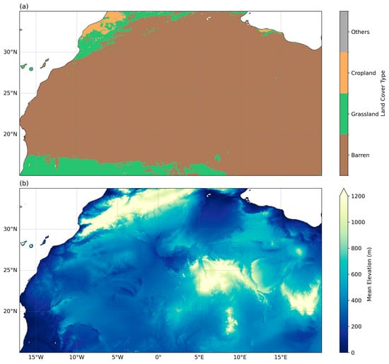
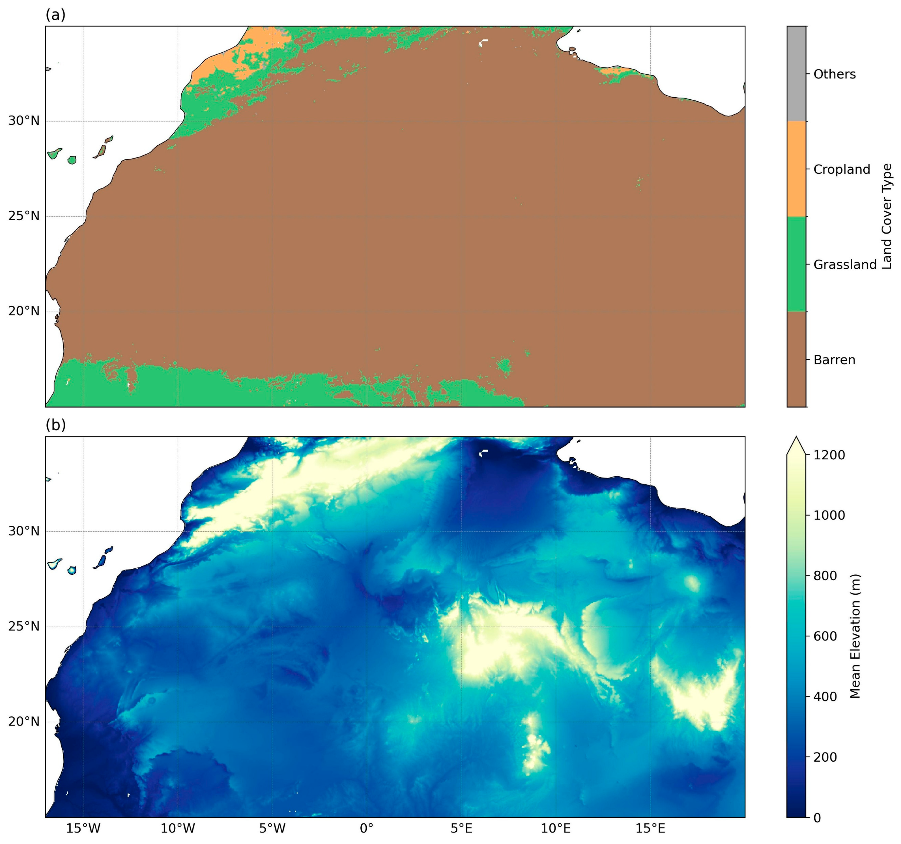
The study area is located in the Sahara region of North Africa, covering 15–35°N and 17°W–20°E. The land surface characteristics are shown in Figure 1. The selection of this region is based on three considerations.

Figure 1. Land cover classification and elevation of the study area: (a) land cover map derived from the 2023 MODIS IGBP classification; (b) mean elevation at a 5 km spatial resolution derived from SRTM data.

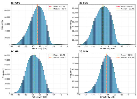
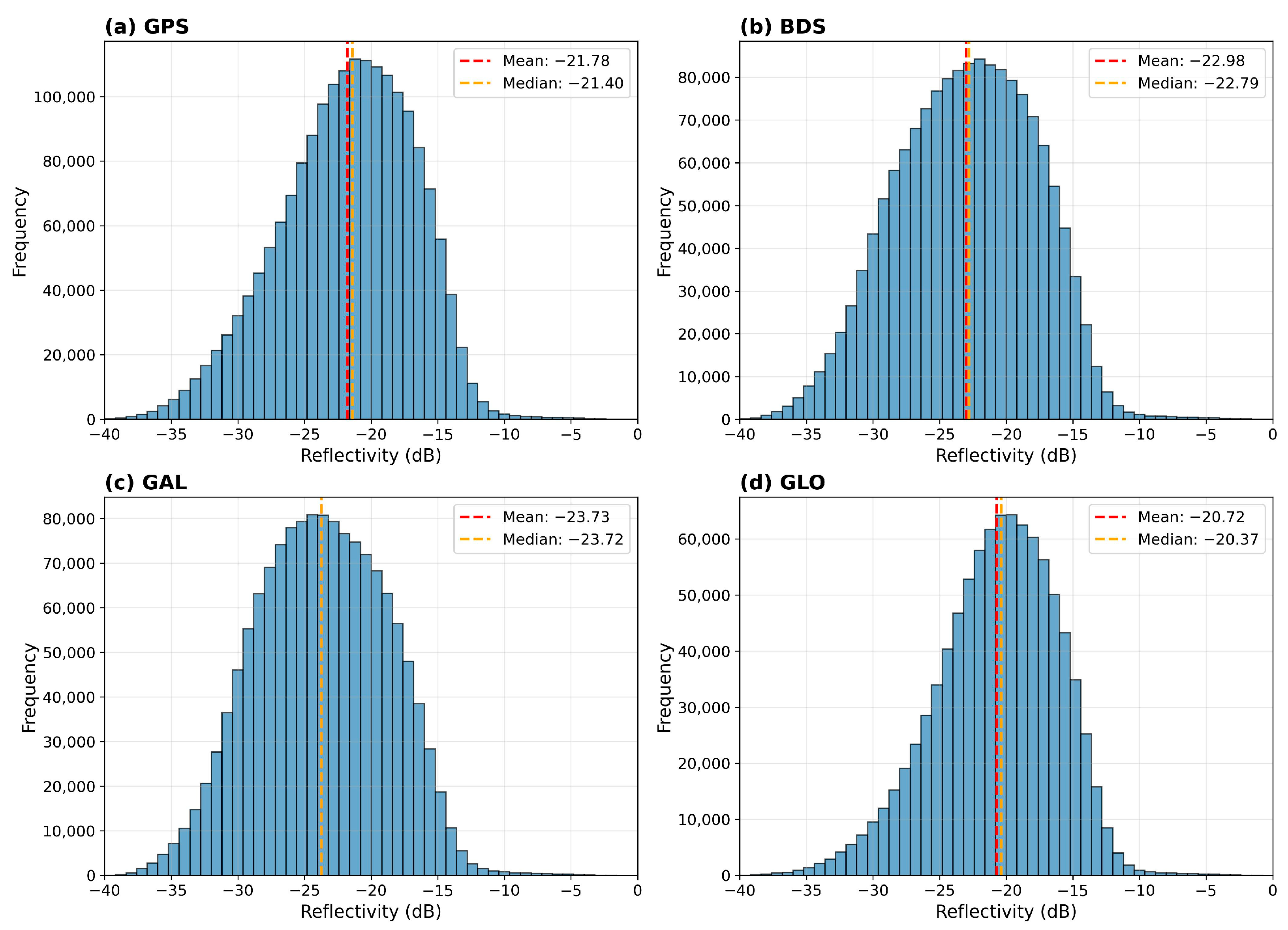
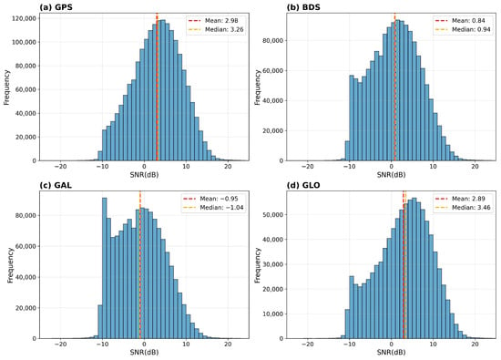
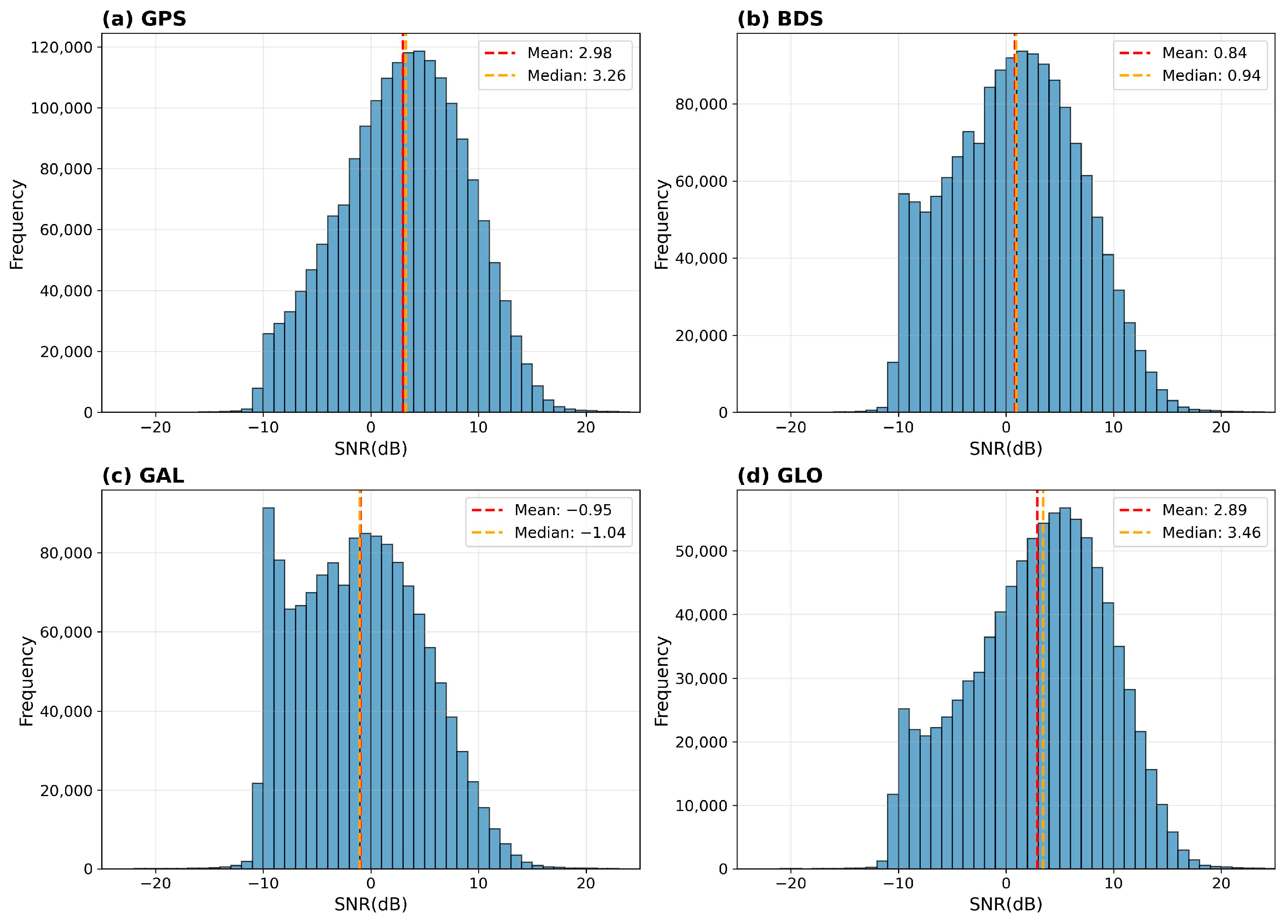
First, both inter-annual and seasonal variability of vegetation cover and soil moisture in this area are low. Second, the surface is relatively smooth, where coherent scattering is expected to dominate. Consistently, the histograms in Figure 2 and Figure 3 indicate relatively high reflectivity and SNR over this region. The mean reflectivity across the four GNSS systems is −22.41 dB, with a corresponding median value of −22.11 dB; the mean SNR is 1.41 dB, with a median value of 1.6 dB. Third, severe radio frequency interference (RFI) has been reported in regions such as the Middle East [28]; selecting the western Sahara can minimize RFI contamination.

Figure 2. Distribution of reflectivity for different GNSS systems over the study area. Statistical distributions of Reflectivity for different GNSS systems over the study area: (a) GPS, (b) BDS, (c) Galileo, and (d) GLONASS. In Figure 2c, the median and mean values are very close and therefore overlap.

Figure 3. Distribution of SNR for different GNSS systems over the study area. Statistical distributions of SNR for different GNSS systems over the study area: (a) GPS, (b) BDS, (c) Galileo, and (d) GLONASS.

2.2. Theoretical Basis

The total received power in the DDM can be described by the Z-V model [29]. Neglecting terms with minor variations such as antenna gain, the DDM observation can be approximated as the convolution of surface scattering and the Woodward ambiguity function (WAF) [9,30,31], as in the following Equation (3):

$$W\left(\tau ,f_D\right)\triangleq {\left|\mathsf{\chi }\left(\mathsf{\tau },{\mathrm{f}}_{\mathrm{D}}\right)\right|}^2 \ast \ast {\left|{\sigma }^0\left(\tau ,f_D\right)\right|}^2$$

(3)

where $W(\tau ,f_D)$ represents the power distribution in delay-Doppler space, $\chi (\tau ,f_D)$ is the Woodward ambiguity function (WAF), ${\sigma }^0(\tau ,f_D)$ is the bistatic radar cross-section (BRCS), “$\mathit{\ast }\mathit{\ast }$” denotes a two-dimensional convolution operation.

Assuming coherent scattering dominates, the reflected signal is mainly concentrated within approximately 1 km around the specular point [32,33], and is governed by the first few Fresnel zones [16]. Under this condition, the DDM shape resembles the WAF itself [9], and can be simplified as Equation (4), as follows:

$$W\left(\tau ,f_D\right)\propto T_c^2·SR·{\left|S\left(f_D\left(\overrightarrow{\rho }\right)-f_c\right)\right|}^2\times {\displaystyle \frac{D^2\left(\overrightarrow{\rho }\right){\mathrm{A}CF}^2\left(\tau -R_r\left(\overrightarrow{\rho }\right)+R_t\left(\overrightarrow{\rho }\right)/c\right)}{{\left(4\pi \left(R_r\left(\overrightarrow{\rho }\right)+R_t\left(\overrightarrow{\rho }\right)\right)\right)}^2}}$$

(4)

where $\tau$ and $f_D$ denote delay and Doppler, $T_c$ is the coherent integration time, $SR$ is surface reflectivity, $S\left(f_D\right)$ is the Doppler-domain spectral response, $f_c$ is the center frequency, $\overrightarrow{\rho }$ is the scattering location vector, $R_r\left(\overrightarrow{\rho }\right)$ and $R_t\left(\overrightarrow{\rho }\right)$ are the distances from the scattering point to the receiver and transmitter, $c$ is the speed of light, $D\left(\overrightarrow{\rho }\right)$ represents the effective antenna footprint in complex amplitude form, and $\mathrm{A}CF(\cdot )$ is the autocorrelation function (ACF). This formulation describes the combined effects of geometry, antenna gain, and signal correlation on the observed DDM.

Under the coherent and spatial concentration assumptions, geometric and antenna terms can be treated as locally constant, and the DDM structure can be further simplified as Equation (5), as follows:

$$ESR\left(\tau ,f_D\right)\propto SR·{\left(WAF\right)}^2$$

(5)

where $\mathrm{E}\mathrm{S}\mathrm{R}(\tau ,f_D)$ denotes the equivalent surface reflectance. Under high coherence, the DDM energy distribution is determined by reflectivity and ${\mathrm{W}\mathrm{A}\mathrm{F}}^2$, which can be further factorized as Equation (6), as follows:

$${\left(\mathsf{\chi }\left(\mathsf{\tau },{\mathrm{f}}_{\mathrm{D}}\right)\right)}^2\approx {\left(ACF\left(\tau \right)\right)}^2·{\left|S\left(f_D\right)\right|}^2$$

(6)

where $\mathrm{A}\mathrm{C}\mathrm{F}\left(\tau \right)$ is the autocorrelation function of the transmitted signal, and $S\left(f_D\right)$ is the Doppler response due to finite integration time. The delay-domain slice of WAF is governed by the ACF, depending on the modulation scheme as Equation (7), as follows:

$$W\left(\tau \right)\propto {\left(ACF\left(\tau \right)\right)}^2$$

(7)

The ACF is given by Equation (8), as follows:

$$ACF\left(\tau \right)=\left\{\begin{array}{c}\mathsf{\Lambda }\left(\tau \right) ,GP{S}_{C/A},GLONAS{S}_{L1OF}\\ {\displaystyle \frac{1}{2}}\left(2\mathsf{\Lambda }\left(\tau \right)-\mathsf{\Lambda }\left(\mathsf{\tau }-1\right)-\mathsf{\Lambda }\left(\tau +1\right)\right),BD{S}_{BOC\left(\mathrm{1,1}\right)},{Galileo}_{BOC\left(\mathrm{1,1}\right)}\end{array}\right.$$

(8)

where $\mathsf{\Lambda }\left(\tau \right)$ is the BPSK (binary phase shift keying) ACF given by Equation (9), as follows:

$$\mathsf{\Lambda }\left(\tau \right)=\left\{\begin{array}{c}1-\left|\tau \right|, \left|\tau \right|\le 1\\ 0, otherwise\end{array}\right.$$

(9)

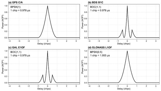
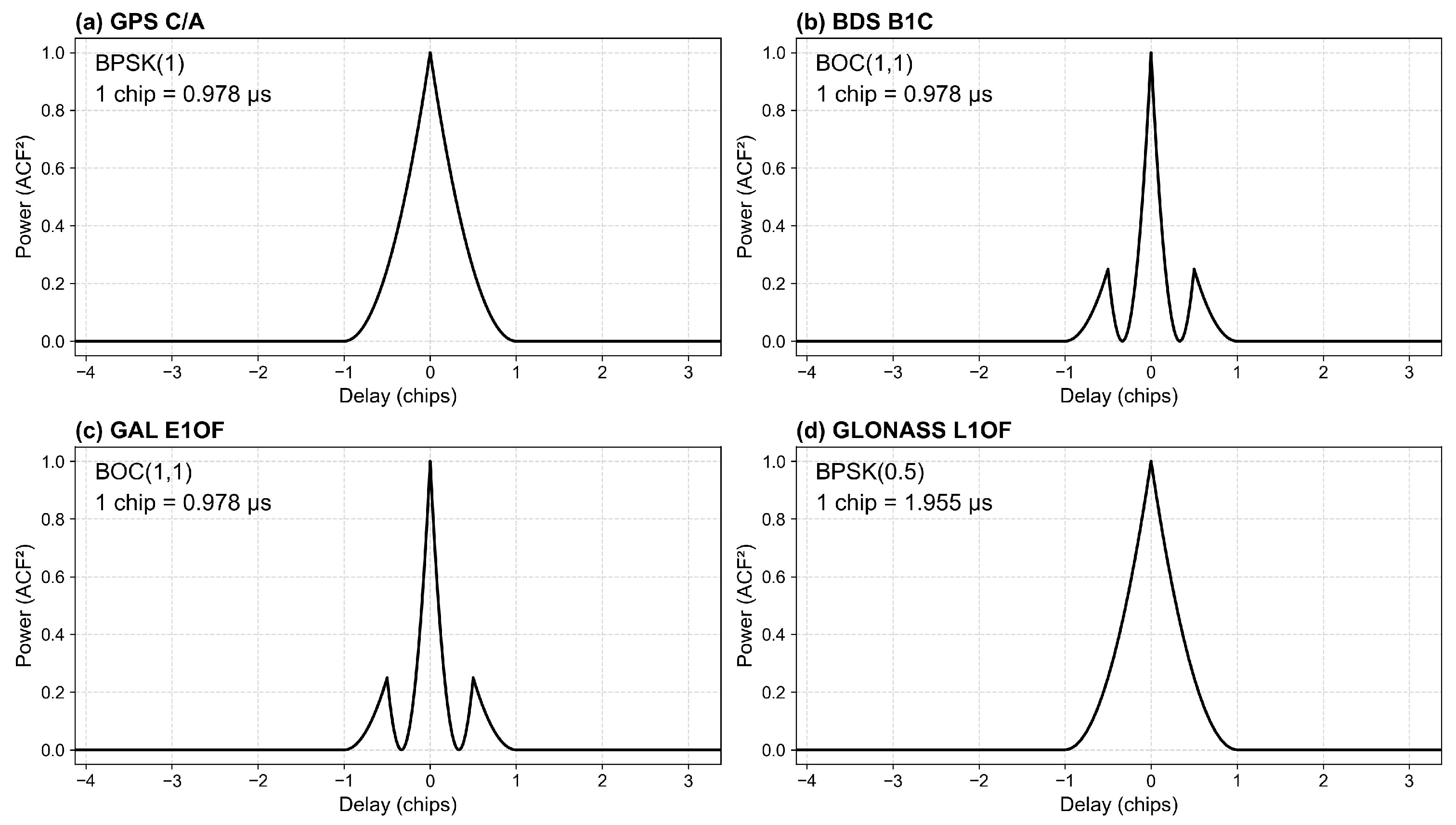
Two points should be noted. First, for GLONASS, the L1OF chip length is approximately twice that of other systems. Although Tianmu-1 uses a uniform delay sampling interval ($\Delta \tau =122.19\hspace{0.17em}\mathrm{n}\mathrm{s}$), this corresponds to different chip resolutions, as follows: 1/8 chip for GPS, BDS, and Galileo, and 1/16 chip for GLONASS. Second, the effect of BOC(6,1) modulation in BDS and Galileo is neglected due to its relatively minor contribution to the overall power distribution. As shown in Figure 4, compared with BPSK signals, BOC (binary offset carrier) modulation exhibits more pronounced sidelobes, with peak sidelobe power approximately 1/4 of the main lobe.

Figure 4. Autocorrelation function (ACF) models for different GNSS systems: (a) GPS, (b) BDS, (c) Galileo, and (d) GLONASS. The ranging code type, modulation scheme, and sampling width are indicated in each panel. BOC(6,1) component is neglected in BDS and Galileo.

In the Doppler domain, $S\left(f_D\right)$ represents the WAF slice along Doppler, with power given by Equation (10), as follows:

$$\mid S\left(f_D\right){\mid }^2={\left|{\displaystyle \frac{\sin \left(\pi f_D{T}_i\right)}{\pi f_D{T}_i}}\right|}^2$$

(10)

where $T_i$ is the coherent integration time, and $f_D$ is the Doppler frequency.

For Tianmu-1, $T_i=1\hspace{0.17em}\mathrm{m}\mathrm{s}$. The Doppler resolution is $\Delta f=500\hspace{0.17em}\mathrm{H}\mathrm{z}$, corresponding to a Doppler range from −5000 Hz to 4500 Hz. In the delay dimension, $\Delta \tau =0.125$ chips for GPS. The total delay window spans from −4.125 chips to 3.375 chips [27].

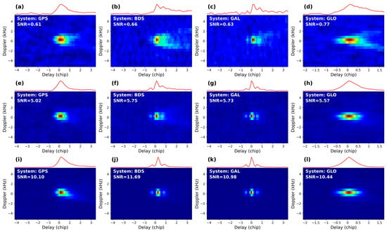
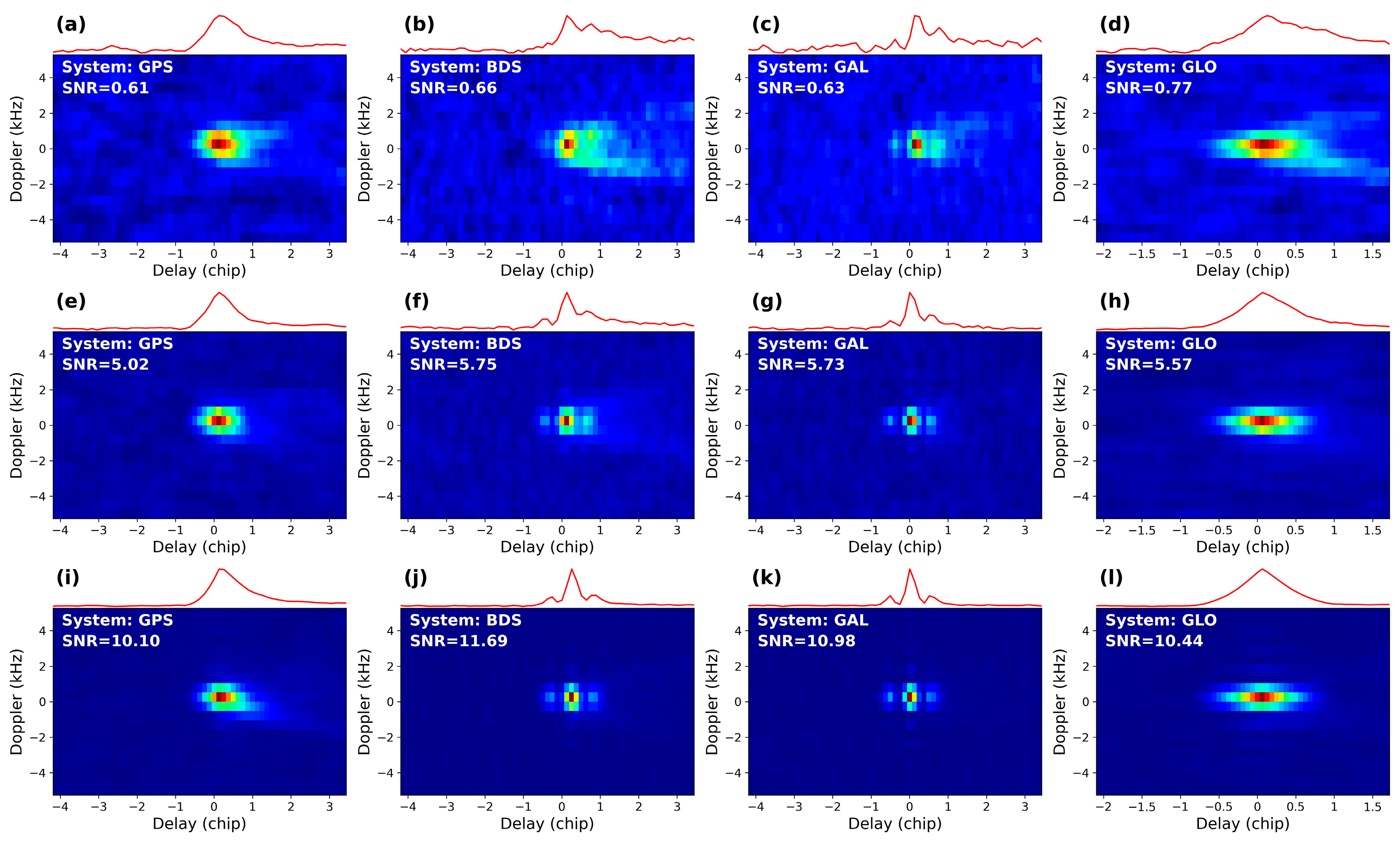
Based on the above, the two-dimensional DDM structure can be interpreted as independent modulations in delay and Doppler. The observed DDMs and corresponding IDWs over the Tianmu-1 are shown in Figure 4. As SNR increases, IDW gradually converges to the ideal delay-domain ACF shown in Equation (6) and Figure 4. In Figure 5i–l, when SNR exceeds 10 dB, IDW closely matches the ideal ACF. For BDS and Galileo, both the amplitude and position of sidelobes are clearly resolved.

Figure 5. DDMs and corresponding IDWs from Tianmu-1 observations under different SNR conditions for multiple GNSS systems. From left to right, the four columns represent GPS, BDS, Galileo, and GLONASS. Panels (a–d) correspond to SNR of 0–1 dB, panels (e–h) to 5–6 dB, and panels (i–l) to SNR > 10 dB. The red line above each DDM represents the IDW obtained by integrating the DDM along the Doppler axis.

3. Characterization of Sampling-Induced Noise in Reflectivity

Under coherent scattering, DDM can be approximated by Equation (4). To analyze noise effects, the Doppler slice at the DDM peak delay is extracted. The IDW-to-DDM peak ratio (IDPR) is defined as Equation (11), as follows:

$$IDPR=IDW\left({\tau }_{peak}\right)/DD{M}_{peak}$$

(11)

where ${DDM}_{\mathrm{peak}}$ denotes the peak power at the specular reflection point. For Tianmu-1, integration along Doppler is expressed as Equation (12), as follows:

$$IDW\left(\tau \right)={\displaystyle \sum _{i=-10}^9}DDM\left(\tau ,i·\Delta f\right)$$

(12)

where $\Delta f=500\hspace{0.17em}\mathrm{H}\mathrm{z}$. When ${\tau }_{\mathrm{peak}}\approx 0$, $\mathrm{A}\mathrm{C}\mathrm{F}\left({\tau }_{\mathrm{peak}}\right)\approx 1$, and the DDM slice as a function of Doppler frequency can be written as Equation (13), as follows:

$$DDM\left(f,0\right)=P_{\mathrm{peak}}\cdot {\left|S\left(f_D\right)\right|}^2$$

(13)

where $P_{\mathrm{peak}}$ denotes the peak power at the specular reflection point. In noise-free conditions, the expression of $\mathrm{I}\mathrm{D}\mathrm{W}\left(0\right)$ is given by Equation (14), as follows:

$$IDW\left(0\right)={\displaystyle \sum _{i=-10}^9}{P}_{peak}·S{\left(i·\Delta f\right)}^2$$

(14)

The ideal waveform is combined with noise to account for realistic conditions. With noise incorporated, IDW(0) can be expressed as Equation (15), as follows:

$$IDW\left(0\right)={\displaystyle \sum _{i=-10}^9}\left(P_{peak}·S{\left(i·\Delta f\right)}^2\right)\oplus noise$$

(15)

Here, the noise floor equivalent power is represented as a unified noise term and combined with the signal component. The combination operator, denoted by $\oplus$, is introduced to characterize the interaction between signal and noise under different assumptions. Specifically, an $L_p$ norm is adopted to provide a unified framework for both quantifying and combining the signal term $P_{peak}·S{\left(i·\Delta f\right)}^2$ and the noise floor equivalent power. The $L_p$ norm is defined as Equation (16), as follows:

$$L_p\left(A,B\right)={\left({\left|A\right|}^p+{\left|B\right|}^P\right)}^{{\displaystyle \frac{1}{p}}}$$

(16)

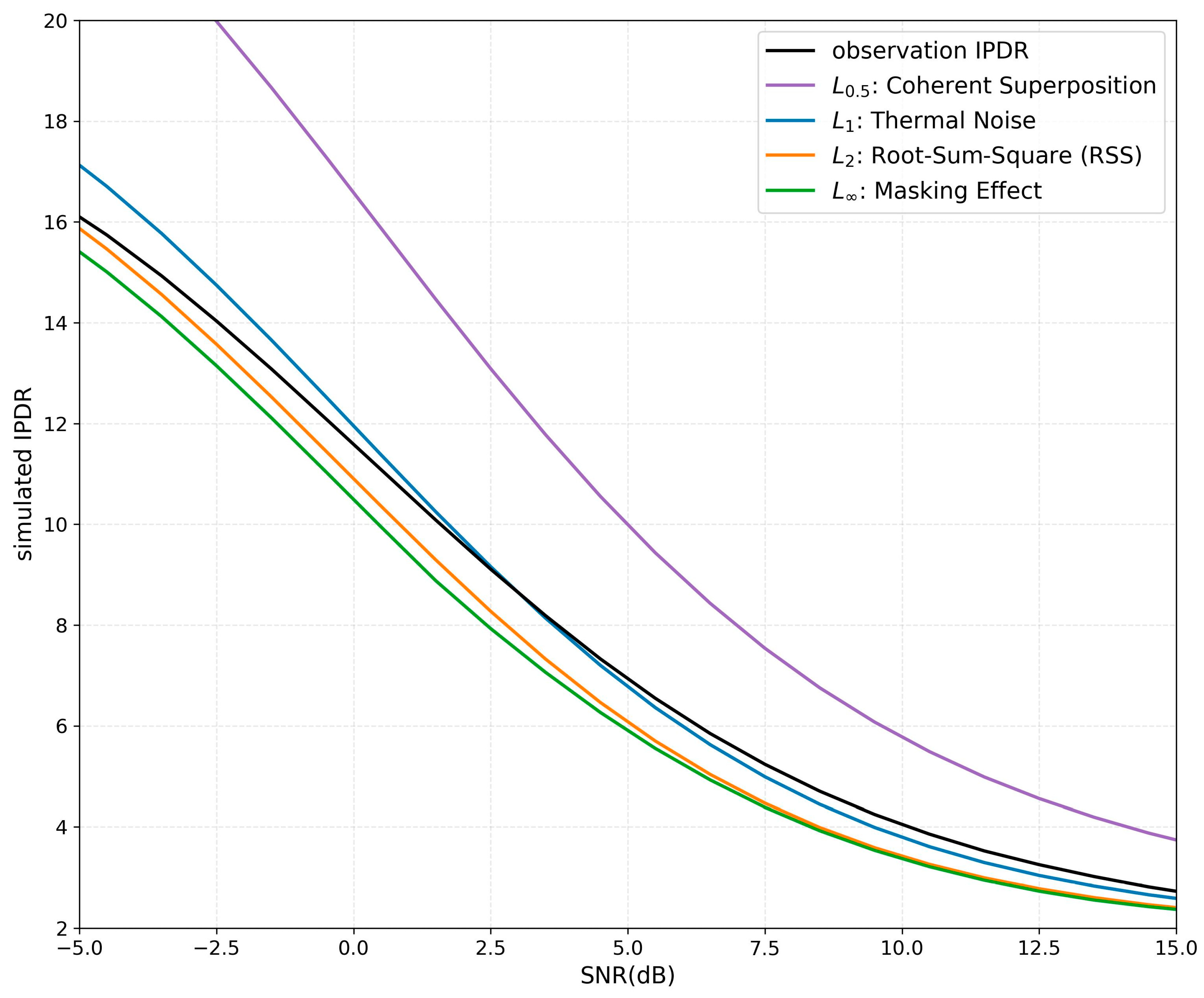
Four strategies are considered by evaluating $L_{0.5}$, $L_1$, $L_2$, and $L_{+\mathrm{\infty }}$. $L_{0.5}$ corresponds to coherent superposition, representing coherent scattering conditions. $L_1$ corresponds to the thermal noise case, where noise can be approximated as an additive background term. $L_2$ represents root-sum-square, where noise and signal are combined geometrically in the power domain. $L_{+\mathrm{\infty }}$ characterizes the masking effect, where the larger value dominates. Based on Equations (11)–(16) and the SNR definition in Equation (2), the simulated IDPR can be expressed as Equation (17), as follows:

$$IDP{R}_{simulated}\left(p,SNR\right)={\sum }_{i=-10}^9{\left({\left|S{\left(i·\Delta f\right)}^2\right|}^p+{\left|{\displaystyle \frac{1}{SNR}}\right|}^p\right)}^{{\displaystyle \frac{1}{p}}}$$

(17)

Since $S(i\cdot \Delta f{)}^2$ is determined by the known Doppler response and remains nearly fixed in this study, $IDP{R}_{simulated}$ is a function of SNR. The simulated $IDP{R}_{L_{0.5}}$, $IDP{R}_{L_1}$, $IDP{R}_{L_2}$, and $IDP{R}_{L_{+\mathrm{\infty }}}$ are then compared with $IDP{R}_{obs}$.

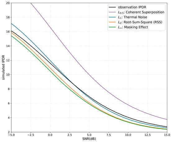
From Figure 6, the simulated IDPR based on the $L_1$-norm noise model ($IDP{R}_{L_1}$) shows the closest agreement with $IDP{R}_{obs}$. This indicates that after 1000 ms incoherent integration, the residual noise in the DDM is dominated by thermal noise, while the coherent component is relatively minor and does not significantly mask the actual scattered signal. As indicated by Equations (1) and (2), the noise floor has already been removed in the engineering processing chain when calculating both SNR and reflectivity in the official Tianmu-1 products. Therefore, the engineering definitions adopted in the Tianmu-1 products are considered reliable, and the results obtained here are consistent with these definitions.

Figure 6. Relationship between IDPR and SNR for both simulated and observed cases under different norms. The black line represents observations, while the simulated results correspond to $L_{0.5}$ (purple), $L_1$ (blue), $L_2$ (orange), and $L_{+\mathrm{\infty }}$ (green) and are calculated based on Equations (11)–(17) using SNR as the only input parameter. The simulated curves theoretically exhibit monotonic relationship between $IDP{R}_{simulated}$ and SNR.

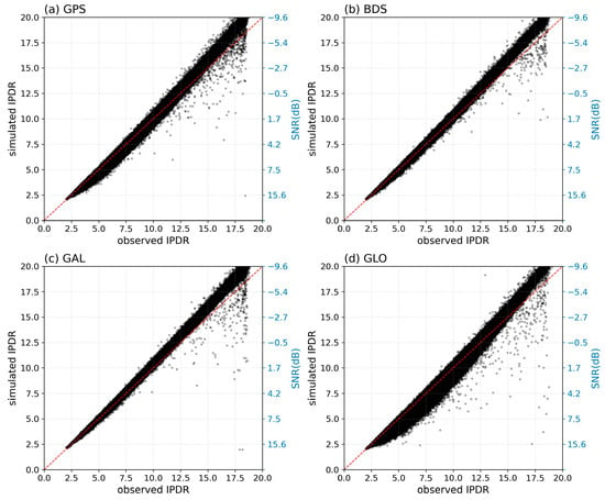
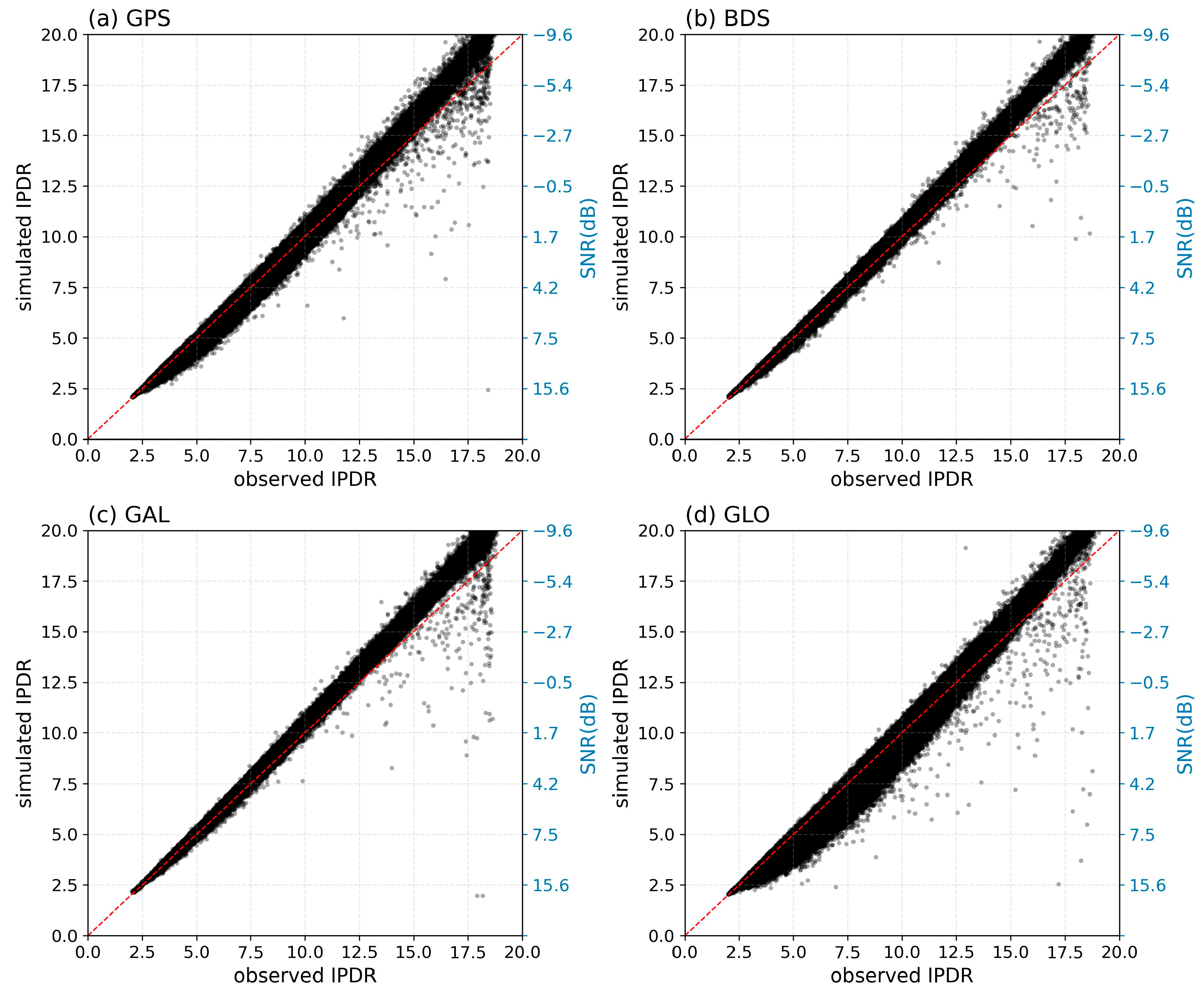
Figure 7 further shows the scatter comparison of $IDP{R}_{L_1}$ among the four GNSS systems. All results are distributed close to the 1:1 reference line, indicating good consistency among different systems after IDW conversion. Although the noise distribution in the original DDM is spatially non-uniform, the IDW is formed through integration over 20 Doppler bins, which significantly improves stability and converts the Doppler-domain noise into an approximately constant background term. Therefore, the subsequent analysis is conducted based on the IDW representation.

Figure 7. Distribution of simulated $IPD{R}_{L1}$ for different GNSS systems. The red dashed line indicates the 1:1 reference line. The right y-axis shows the corresponding SNR scale.

The relationship between $IDW\left(\tau \right)$ and $DDM(\tau ,f_D)$ can be approximated based on the WAF formulation. The DDM can be approximately expressed as follows:

$$DDM\left(\tau ,f_D\right)\approx P_{peak}·{\chi }^2\left(\tau ,f_D\right)+N\left(\tau ,f_D\right)$$

(18)

where $N(\tau ,f_D)$ represents the additive noise term. According to the previous analysis, this term is mainly dominated by thermal noise.

According to Equations (6) and (10), the delay and Doppler dimensions of the WAF can be regarded as approximately independent near the specular point. Since the IDW is obtained by integrating the DDM along the Doppler dimension,

$$IDW\left(\tau \right)\approx P_{peak}·{\left(ACF\left(\tau \right)\right)}^2\sum _{f_D}{\left|S\left(f_D\right)\right|}^2+C$$

(19)

where $C$ represents the integrated background component introduced by thermal noise and other non-ideal terms. Because the IDW is generated from summation over 20 Doppler bins, $C$ can be approximately regarded as 20 times the noise floor.

For Tianmu-1, the Doppler sampling range is $-4500\sim 5000$ Hz with $T_c=1 \mathrm{ms}$. According to Equation (10),

$$k={\displaystyle \sum _{f_D=-4500}^{5000}}{\left|S\left(f_D\right)\right|}^2\approx 1.96$$

(20)

which can be treated as approximately constant within the effective WAF region. Thus,

$$IDW\left(\tau \right)\approx k·P_{peak}·{\left(ACF\left(\tau \right)\right)}^2+C$$

(21)

The noise-free IDW is then given by the following:

$$ID{W}_{nf}\left(\tau \right)\approx k·P_{peak}·{\left(ACF\left(\tau \right)\right)}^2$$

(22)

Therefore, for arbitrary delay positions ${\tau }_1$ and ${\tau }_2$,

$${\displaystyle \frac{ID{W}_{nf}\left({\tau }_1\right)}{ID{W}_{nf}\left({\tau }_2\right)}}\approx {\displaystyle \frac{k·P_{peak}·{\left(ACF\left({\tau }_1\right)\right)}^2}{k·P_{peak}·{\left(ACF\left({\tau }_2\right)\right)}^2}}={\displaystyle \frac{{\left(ACF\left({\tau }_1\right)\right)}^2}{{\left(ACF\left({\tau }_2\right)\right)}^2}}$$

(23)

Furthermore, for the original DDM after background noise removal,

$${\displaystyle \frac{DDM\left({\tau }_1,f_D\right)-N}{DDM\left({\tau }_2,f_D\right)-N}}\approx {\displaystyle \frac{{\left(ACF\left({\tau }_1\right)\right)}^2}{{\left(ACF\left({\tau }_2\right)\right)}^2}}\approx {\displaystyle \frac{\mathsf{\Gamma }\left({\mathsf{\tau }}_1\right)}{\mathsf{\Gamma }\left({\mathsf{\tau }}_2\right)}}$$

(24)

After background noise removal, the ratio relationship derived from the original DDM is approximately equivalent to that derived from the IDW. Since the official Tianmu-1 reflectivity product is calculated from the noise-floor-removed DDM peak, the reflectivity correction can be expressed using the same multiplicative factor derived from the IDW representation.

4. Impact of Delay-Domain Discretization on Peak Estimation

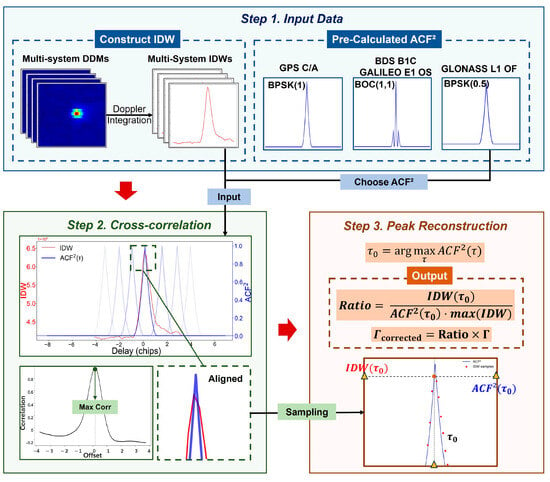
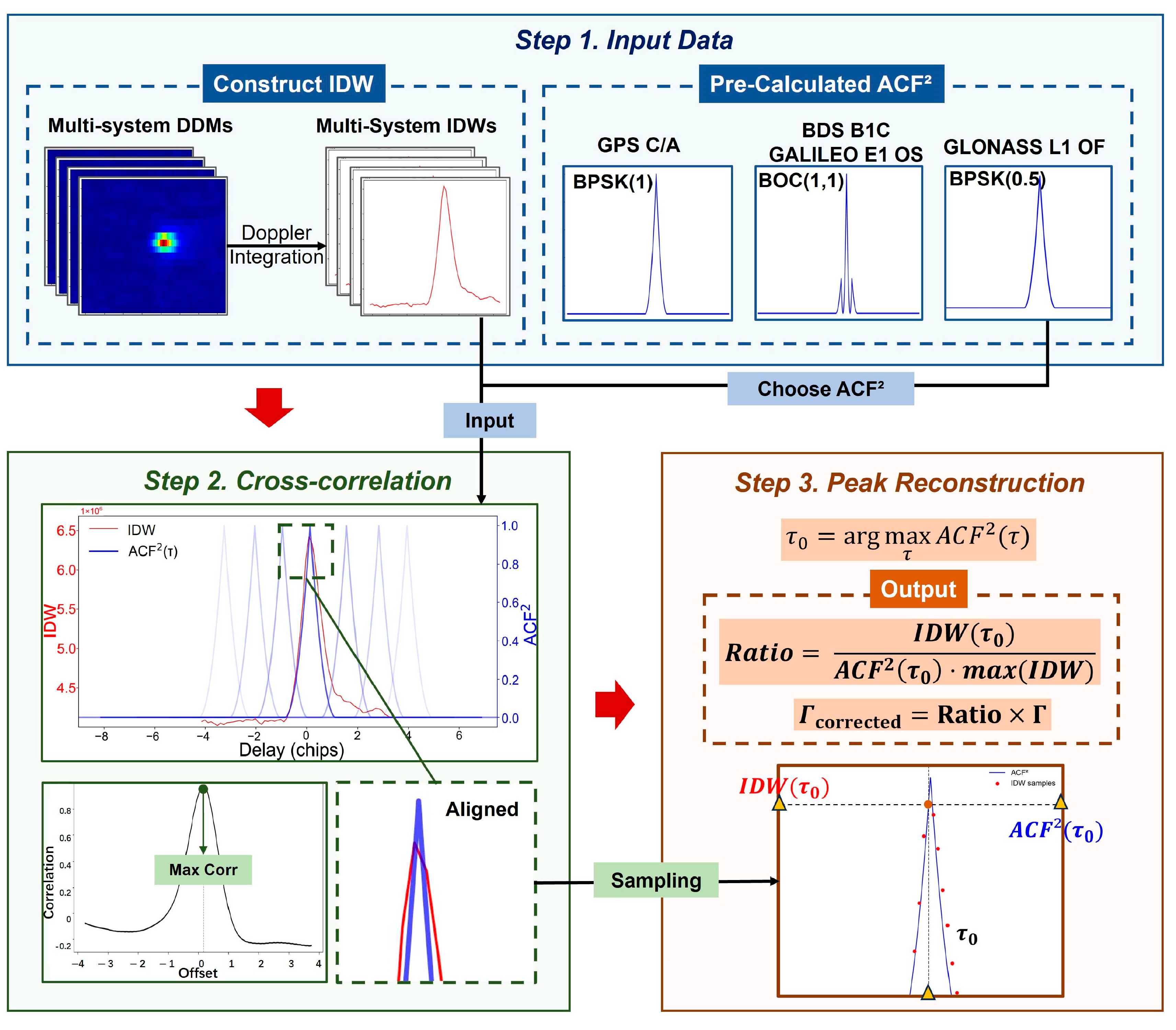
Based on the analysis in Section 3, the original DDM(τ) is integrated along the Doppler dimension to obtain IDW(τ), which is then used to evaluate delay bias and recover the underestimated reflectivity. Tianmu-1 observations include four GNSS systems: GPS, BDS, GLONASS, and Galileo. The ACFs of BDS and Galileo signals exhibit pronounced sidelobe structures. A cross-correlation-based alignment method is adopted, as illustrated in Figure 8, consisting of the following three steps: (1) construction of an ideal ${\mathrm{A}\mathrm{C}\mathrm{F}}^2$ template; (2) alignment between IDW and the template using cross-correlation; and (3) reconstruction of peak power using a correction factor at the aligned position (as defined in Equation (26)).

Figure 8. Flowchart of the peak power reconstruction method. The method consists of delay alignment, sub-chip delay estimation, and peak power correction based on the Ratio factor.

The cross-correlation between IDW(τ) and ${\mathrm{A}\mathrm{C}\mathrm{F}}^2\left(\tau \right)$ is computed as Equation (25) [34], as follows:

$${\rho }_{ACF,IDW}\left(\Delta \tau \right)={\displaystyle \frac{\sum \left(IDW\left(\tau \right)\cdot AC{F}^2\left(\tau +\Delta \tau \right)\right)}{\sqrt{\sum ID{W}^2\left(\tau \right)\cdot \sum AC{F}^4\left(\tau +\Delta \tau \right)}}}$$

(25)

The optimal alignment is achieved when the cross-correlation coefficient reaches its maximum. At this point, the intercept term in the fitting can be approximated as a residual thermal noise component. According to Equation (1), thermal noise has already been removed in the Tianmu-1 official product. Since each IDW sample can be approximated as the original signal with an added constant background (approximately noise floor × 20), the intercept term is neglected under this assumption.

Based on the alignment, the ratio between IDW and ${\mathrm{A}\mathrm{C}\mathrm{F}}^2$ at the corresponding delay is used to reconstruct the peak as Equation (26), as follows:

$${IDW}_{\mathrm{recons}}={\displaystyle \frac{IDW\left({\tau }_0\right)}{AC{F}^2\left({\tau }_0\right)}}$$

(26)

where ${IDW}_{\mathrm{recons}}$ represents the reconstructed IDW peak. Based on ${IDW}_{\mathrm{recons}}$ and the original ${IDW}_{\mathrm{peak}}$, a correction factor IPR is defined as Equation (27), as follows:

$$IPR={\displaystyle \frac{ID{W}_{recons}}{ID{W}_{peak}}}$$

(27)

According to Equations (22) and (23) and the official reflectivity definition in Equation (1), it can be approximately expressed as follows:

$$IP{R}_{IDW}\approx IP{R}_{ref}$$

(28)

The corrected reflectivity is then obtained by applying this factor as Equation (29), as follows:

$${\mathsf{\Gamma }}_{corrected}=IPR\times \mathsf{\Gamma }$$

(29)

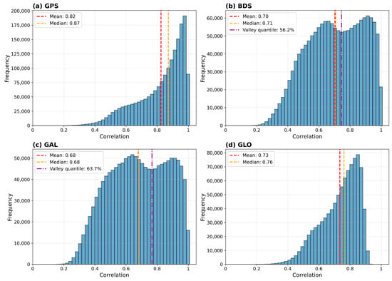
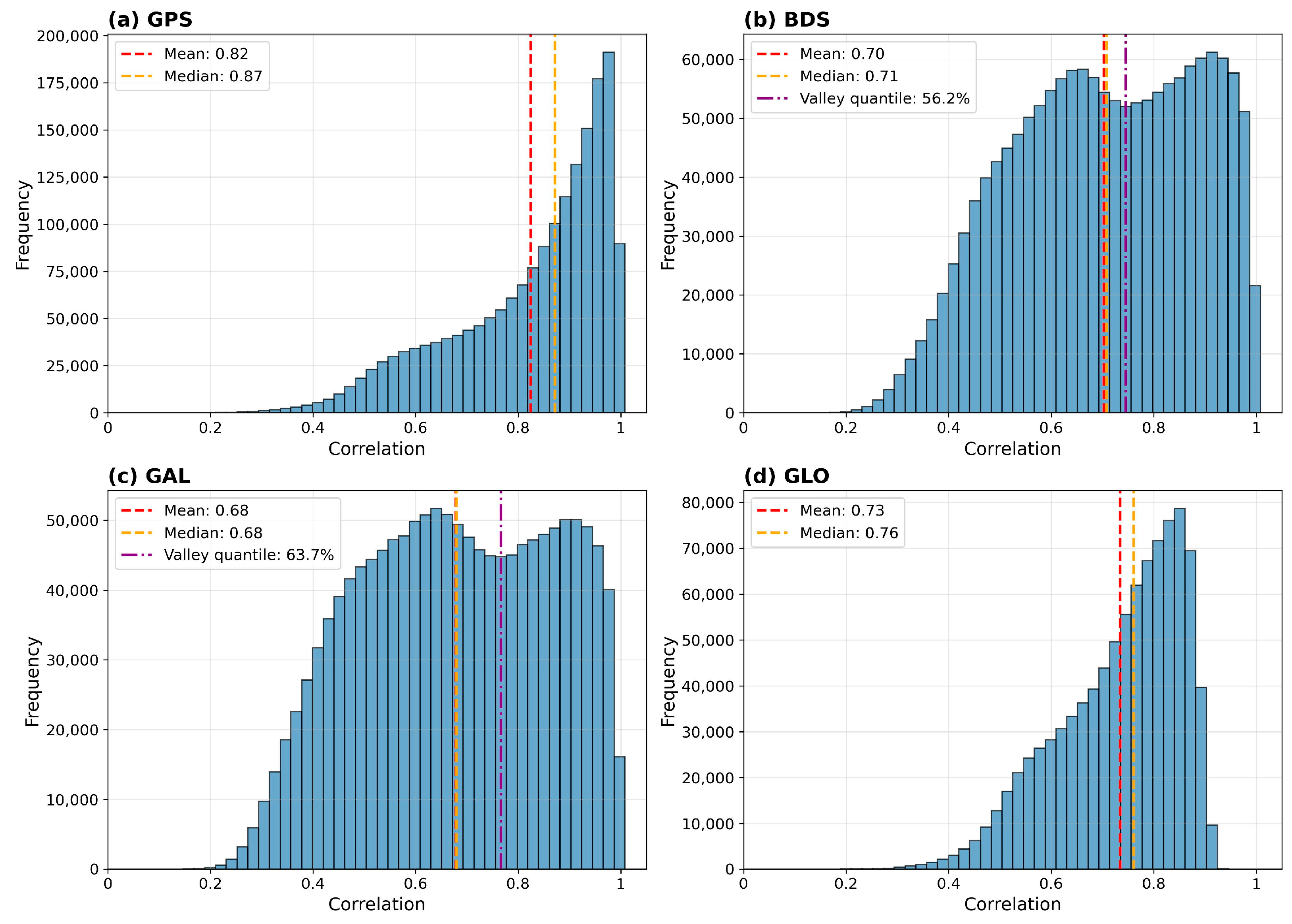
Histograms of the correlation coefficients obtained from the cross-correlation analysis are presented in Figure 9. The correlation coefficient distributions of the BOC(1,1)-modulated signals exhibit a bimodal pattern due to the presence of sidelobes in the correlation function. The minima between the two peaks correspond approximately to the 60th percentile of the reflectivity distributions for the BDS and Galileo systems. Beyond this point, higher correlation coefficients generally indicate the emergence of two visible sidelobes in the IDW, implying stronger coherence. The corresponding mean reflectivity value averaged over the four GNSS systems is approximately −20.73 dB. Although the BPSK-modulated signals do not exhibit a similar minimum, coherence is not fundamentally dependent on the ranging code type. Therefore, the same 60th-percentile criterion was uniformly adopted in the subsequent analysis, corresponding to a reflectivity threshold of −20 dB.

Figure 9. Distribution of correlation coefficients after cross-correlation for different GNSS systems. Histograms of correlation coefficients after cross-correlation for different GNSS systems: (a) GPS, (b) BDS, (c) Galileo, and (d) GLONASS.

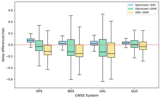
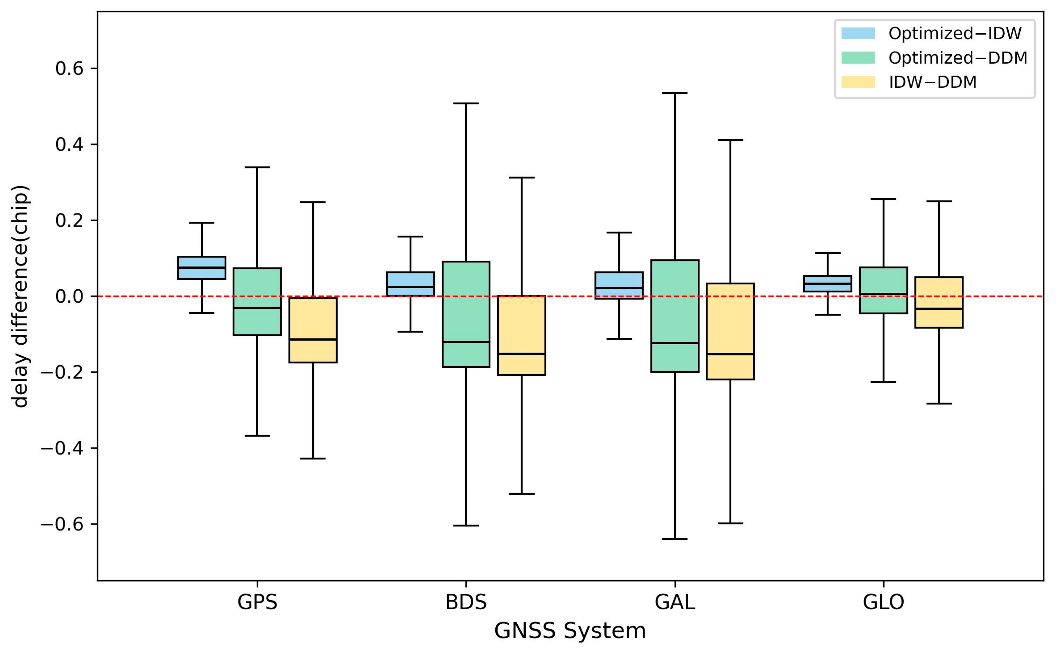
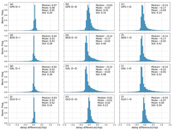
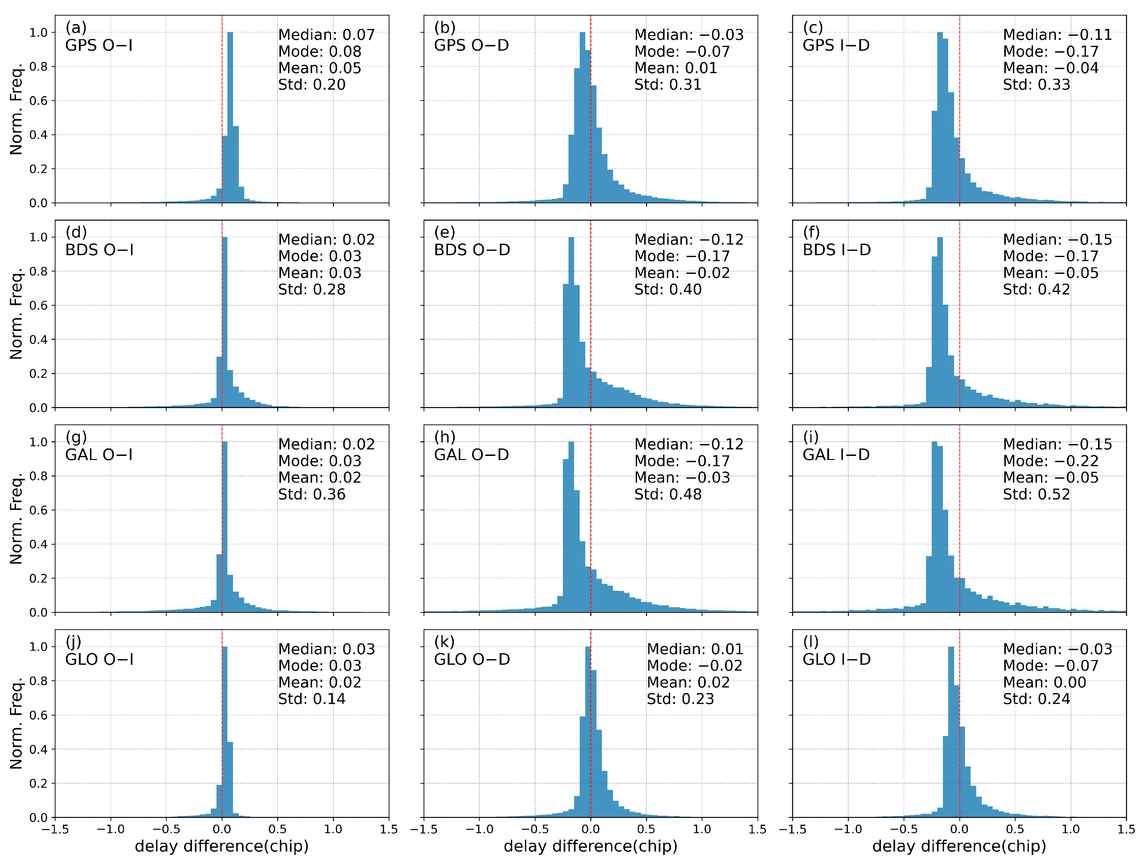
Compared with the delay corresponding to the original DDM peak, the retrieved optimized specular delay shows an overall negative bias, indicating that the original DDM peak position is systematically delayed. Figure 10 and Figure 11 show that for GPS, BDS, and Galileo, the optimized specular delay exhibits a clear negative bias relative to the DDM peak delay, approximately −0.02 to −0.17 chips. For GLONASS, the bias is −0.02 with a standard deviation of 0.23, representing the smallest deviation and a distribution concentrated near zero delay. The higher delay sampling resolution of GLONASS (1/16 chip) reduces discretization error. Signals with BOC modulation, however, have steeper correlation function slopes and are more sensitive to sampling errors, leading to larger standard deviations for BDS and Galileo (0.40 and 0.48, respectively).

Figure 10. Boxplots of delay bias for different GNSS systems. Blue represents optimized specular point delay minus IDW peak delay, green represents optimized specular point delay minus DDM peak delay, and yellow represents IDW peak delay minus DDM peak delay.

Figure 11. Histograms of delay difference across GNSS systems. O−I denotes optimized specular point delay minus IDW peak delay; O−D denotes optimized specular point delay minus DDM peak delay; and I−D denotes IDW peak delay minus DDM peak delay. GAL: Galileo; GLO: GLONASS. The blue bars represent the delay difference, and the red dashed line represents the zero level.

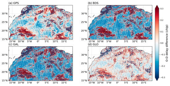
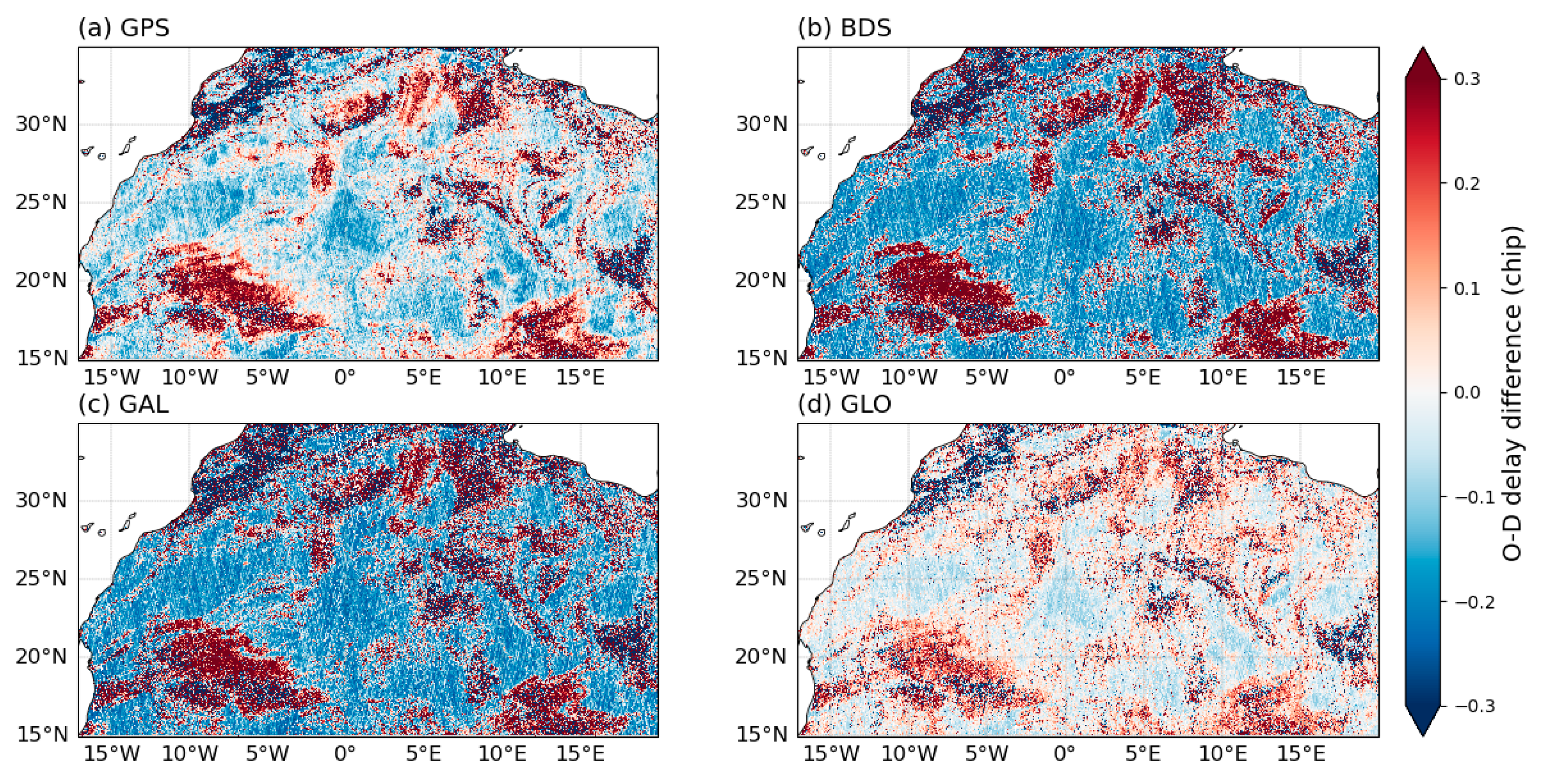
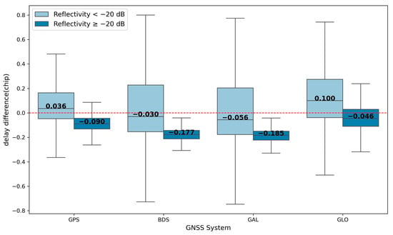
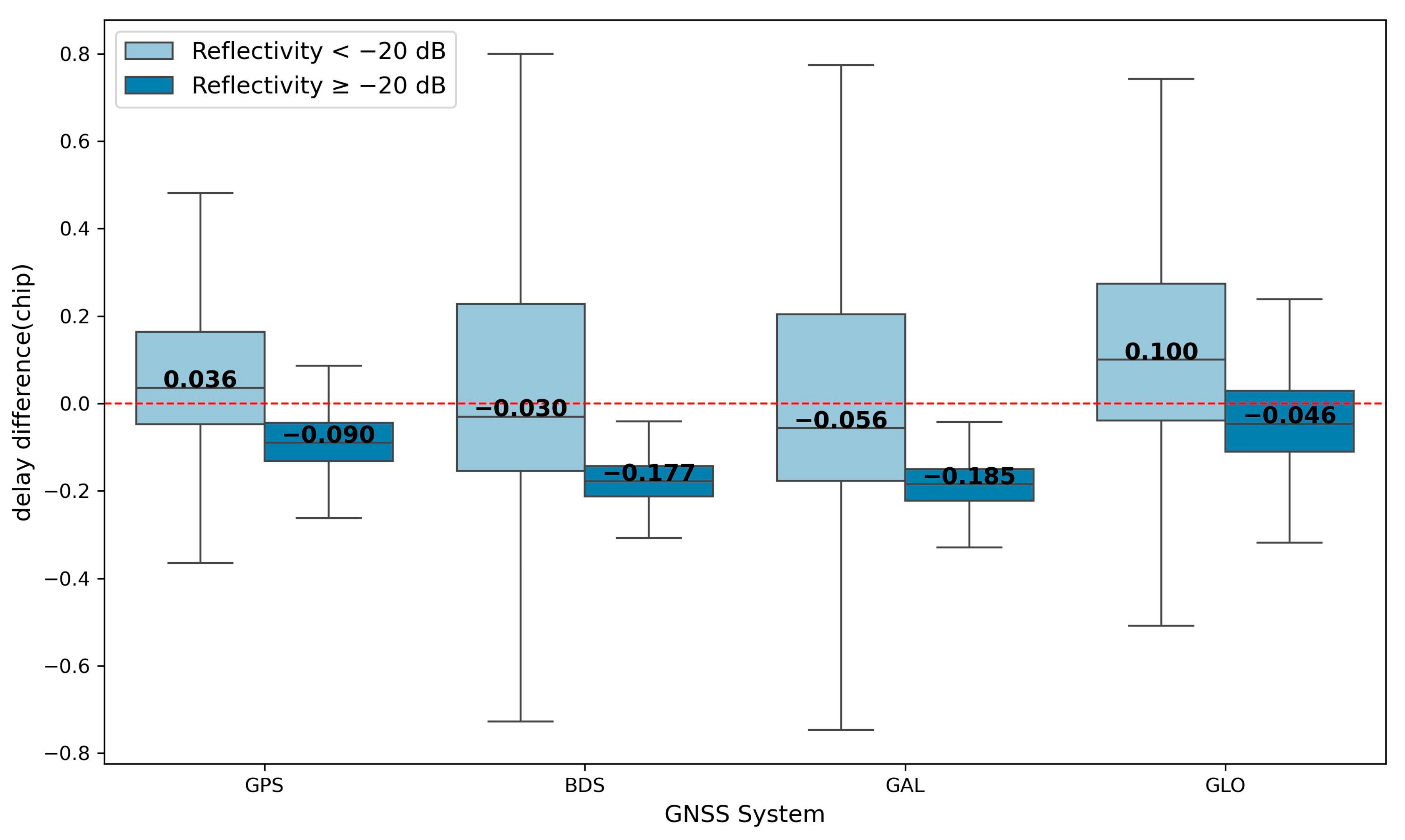
From the spatial distribution (Figure 12), the standard deviation of delay differences increases significantly under low reflectivity conditions. In Figure 13, a threshold of −20 dB is used to separate high and low reflectivity regimes. When reflectivity is below −20 dB, the standard deviations of delay differences range from 0.38 to 0.58, with GPS showing the lowest standard deviation. When reflectivity exceeds −20 dB, the delay bias becomes relatively stable, ranging from −0.185 to −0.046 chips. This behavior is associated with lower SNR under low reflectivity conditions, where increased noise amplifies sampling-induced errors.

Figure 12. Spatial distribution of optimized specular point delay minus DDM peak delay for each GNSS system: (a) GPS; (b) BDS; (c) Galileo (GAL); (d) GLONASS (GLO).

Figure 13. Boxplots of delay difference across GNSS systems. The data are grouped by reflectivity, with −20 dB as the threshold separating high and low reflectivity conditions.

A comparison of different processing methods (Figure 10 and Figure 11) shows that the delay difference between the IDW peak and the DDM peak exhibits large negative bias, ranging from −0.22 to −0.07 chip. This result indicates that IDW has an earlier peak. In contrast, the optimized specular point delay exhibits a positive bias relative to the IDW peak delay, ranging from 0.03 to 0.08 chip, suggesting that the reconstructed peak is slightly delayed relative to the IDW peak. The optimized specular point delay lies between the IDW peak delay and the DDM peak delay, providing a more balanced estimate of the delay.

5. Reflectivity Correction

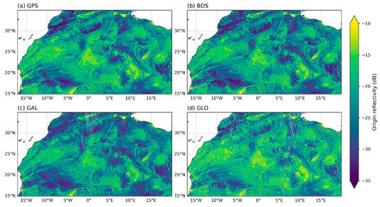
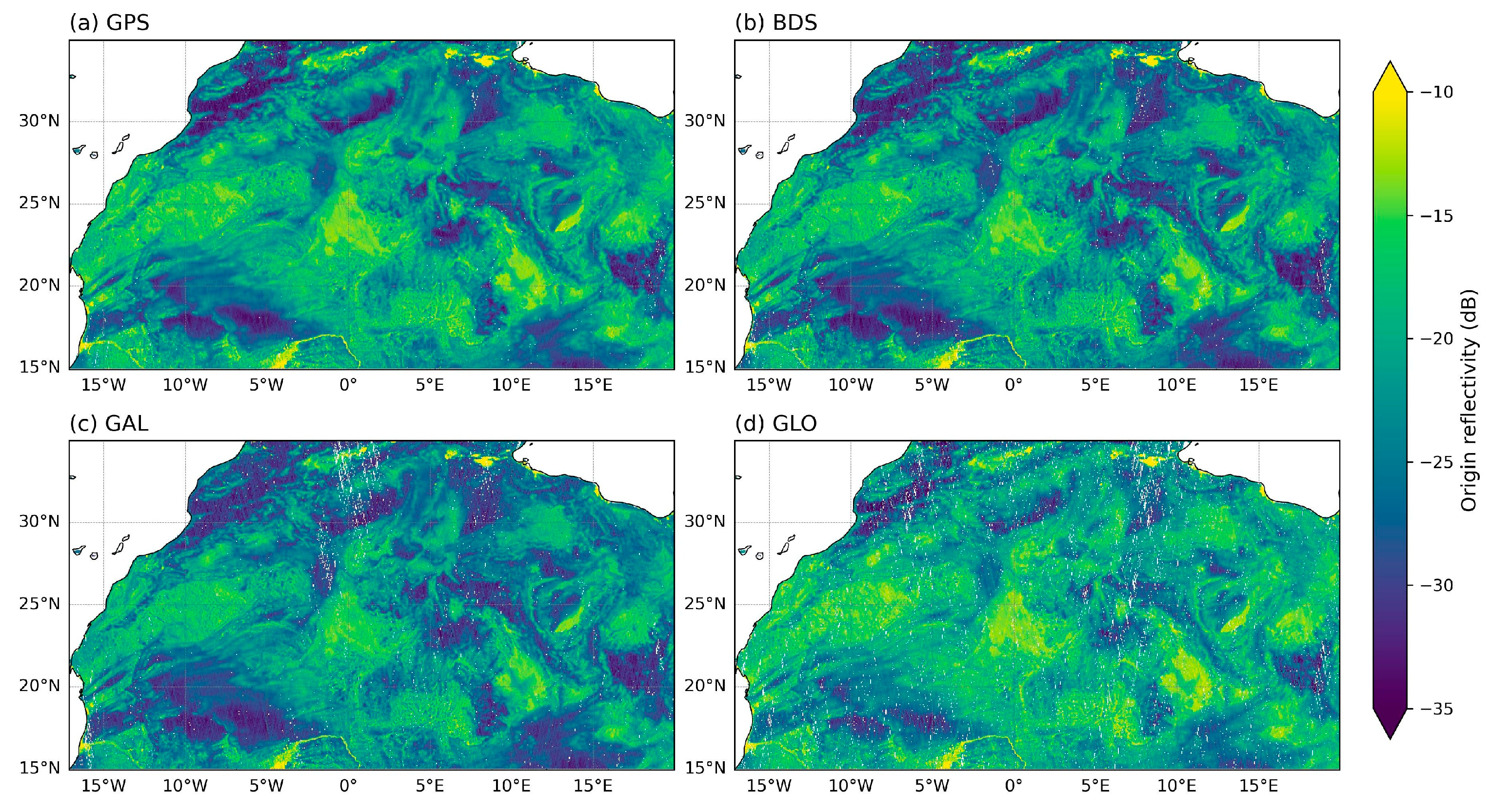
This section evaluates the reflectivity corrected according to Equation (28). The annual average reflectivity for each GNSS system is shown in Figure 14.

Figure 14. Reflectivity in the study area. Reflectivity is expressed in dB. (a) GPS; (b) BDS; (c) Galileo; (d) GLONASS.

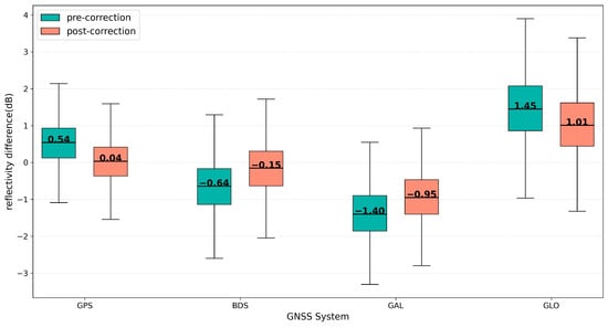
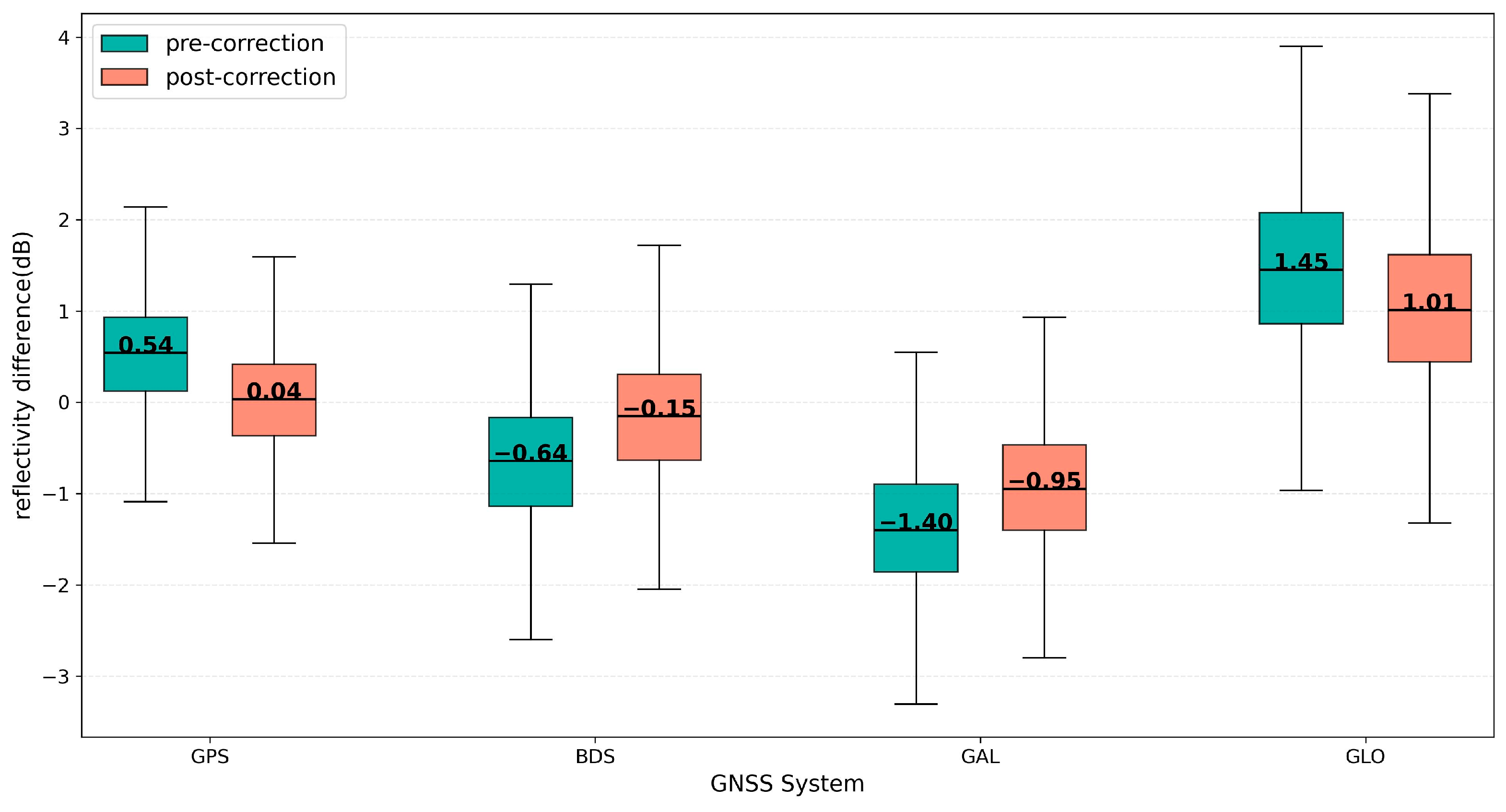
The original reflectivity exhibits a systematic underestimation. The bias is approximately 0.4 dB for GPS and GLONASS, while BDS and Galileo show larger underestimation of about 1.3 dB (see Table 1 for details). Compared with previous studies, DDMA observations from FY-3E & FY-3F show an overall overestimation of 0.5–1.1 dB [24]. By comparison, the results in this study indicate underestimation, with clearer inter-system differences. As shown in Figure 15, the differences between each system and the mean reflectivity are reduced after correction, with changes of approximately 0.5 dB. After our correction, the consistency among different systems is significantly improved.

Table 1. IPR in reflectivity (Unit: dB).

GPS	BDS	Galileo	GLONASS
0.37 ± 0.15	1.35 ± 0.39	1.31 ± 0.43	0.43 ± 0.11

Figure 15. Reflectivity difference of each GNSS system relative to the mean reflectivity before and after correction. The difference is defined as the system-specific reflectivity minus the corresponding mean reflectivity (before and after correction, respectively), with all values expressed in dB.

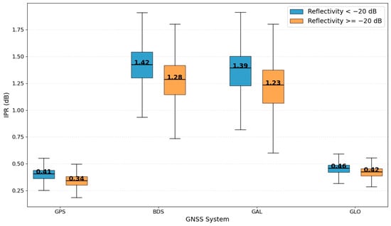
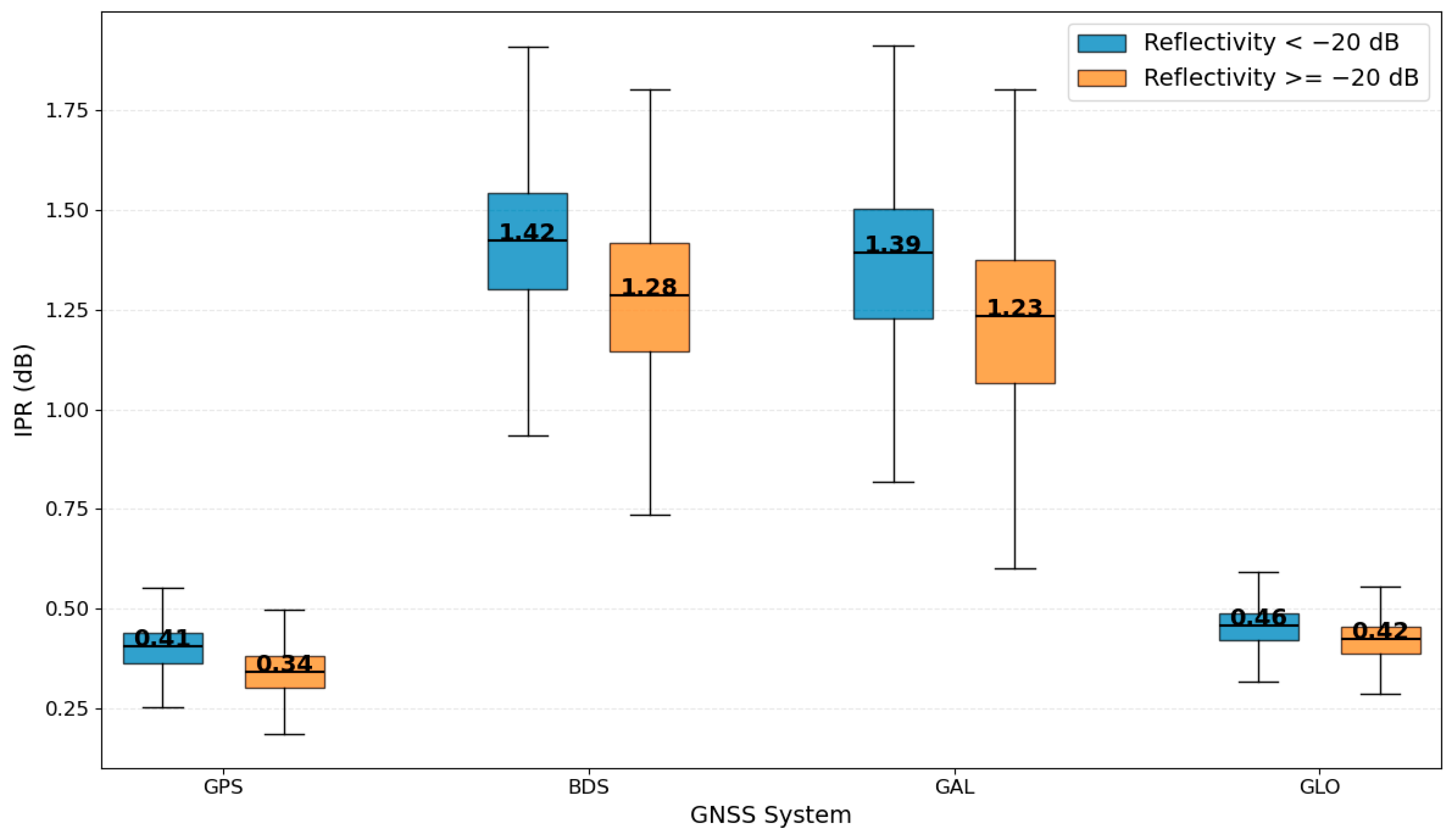
The distribution of IPR is closely related to reflectivity levels. Figure 16 shows the system-wise distribution of IPR under different reflectivity conditions. Within each reflectivity range, IPR for GPS and GLONASS remains relatively stable between 0.3 and 0.5 dB, while BDS and Galileo are mainly distributed between 1.2 and 1.5 dB, consistent with the overall statistics in Table 1.

Figure 16. Boxplots of IPR for different GNSS systems under varying reflectivity conditions. IPR is grouped using a −20 dB reflectivity threshold, and its definition follows Equation (18) and is expressed in dB.

As reflectivity decreases, IPR shows an increasing trend, indicating that the correction magnitude becomes larger under low reflectivity conditions. This behavior is associated with lower SNR, where the impact of delay-domain discretization on peak localization and amplitude estimation becomes more pronounced, leading to stronger underestimation and larger IPR corrections.

The differences among systems are closely related to signal structures. On the one hand, BDS and Galileo signals with BOC modulation have sharper ACF main lobes, making them more sensitive to discretization effects and more prone to peak estimation bias. On the other hand, GLONASS benefits from a higher delay sampling resolution, allowing a more accurate representation of the peak structure and reducing reflectivity estimation errors induced by sampling effects. Under discrete delay sampling conditions, sharper waveform structures are more sensitive to sampling offsets because the sampled peak may deviate more significantly from the actual waveform maximum. As a result, the discretization-induced delay bias and reflectivity underestimation become more pronounced for BDS and Galileo than for GPS and GLONASS. In contrast, the broader waveform structures of GPS and GLONASS reduce the sensitivity to discrete sampling intervals and therefore improve the stability of peak localization. In addition, potential influences from receiver-side processing and onboard DDM generation strategies in Tianmu-1 cannot be completely excluded and may also contribute to part of the observed inter-system differences.

6. Discussion

This study presents a preliminary assessment of sampling-induced bias in multi-GNSS reflectivity observations. The analysis is based on several simplifying assumptions, including idealized waveform representation and coherent scattering conditions over relatively homogeneous desert surfaces, which may limit the generality of the results. These factors should be considered when interpreting the presented results.

The inter-system discrepancy may be related not only to signal structure, but also to the sensitivity of the peak localization algorithm to different ranging codes. The reconstruction in this study is based on a maximum-correlation strategy, while BPSK-like and BOC-modulated signals have different autocorrelation structures. BPSK signals have broader main lobes and generally higher correlation coefficients, whereas BOC(1,1) signals contain sharper peak structures and sidelobes, making the localization process more sensitive to discrete sampling. In the current implementation, the maximum correlation peak is directly selected without distinguishing the sensitivity of the cross-correlation process for different signal types. This may also contribute to the observed discrepancy between BPSK-like and BOC-modulated signals.

The proposed correction mainly improves the relative consistency among different GNSS systems, but residual inter-system reflectivity differences still remain after correction. BPSK-like signals still tend to exhibit relatively higher reflectivity, whereas BOC-modulated signals remain systematically lower. At the current stage, it is difficult to determine whether the remaining discrepancy mainly originates from residual sampling-induced bias or from systematic calibration uncertainties within the observation system, such as EIRP uncertainty and inter-system calibration inconsistency. Since these effects are coupled in the current observations, the present analysis cannot completely separate the contribution of discrete sampling from other instrumental factors.

The present analysis is mainly conducted over desert regions with minimal vegetation cover and weak seasonal variability, in order to reduce the influence of surface heterogeneity on the observed signal and better isolate the sampling-related effects. When extending the proposed method to more complex land surfaces, such as vegetated or dynamically changing regions, additional adaptations or refinements may be required.

This study mainly focuses on the relative consistency of reflectivity among different GNSS systems rather than the absolute accuracy of reflectivity itself. Absolute validation of land reflectivity under coherent scattering conditions remains difficult, and it is therefore challenging to determine which GNSS system provides reflectivity values closest to the true surface response. The current analysis mainly aims to characterize the relative impact of discrete sampling on multi-GNSS reflectivity consistency.

7. Conclusions

This study quantitatively evaluates the impact of DDM discrete sampling on GNSS-R land reflectivity retrieval. A cross-correlation method based on an ideal ${\mathrm{A}\mathrm{C}\mathrm{F}}^2$ template is used for delay alignment and peak reconstruction. The main conclusions are as follows:

• The optimized specular point delay shows an overall advance relative to the original DDM peak delay, approximately 0.02 chips for GPS and GLONASS, and 0.17 chips for BDS and Galileo.
• A systematic underestimation is observed in the corresponding reflectivity, with BDS and Galileo showing biases of about 1.4 dB.

These results suggest that peak localization bias induced by discrete delay sampling is likely an important contributor to reflectivity underestimation. The correction proposed in this study reduces the relative differences in reflectivity observations among the four GNSS systems. From the comparison between simulation and observation in the Doppler slice, the observation noise is mainly characterized as additive thermal noise, which has already been removed in the Tianmu-1 official reflectivity product and has a limited impact on the above conclusions.

The results provide a quantitative basis for characterizing the effects of discrete sampling errors on delay estimation and reflectivity retrieval, and contribute to improving the consistency and comparability among multi-GNSS observations. The findings can support the refinement of GNSS-R data processing methods and the design of sampling strategies. Under land coherent scattering conditions, they may help reduce systematic underestimation and improve reflectivity retrieval accuracy. The results also indicate that the current DDM sampling strategy has limitations under such conditions, and higher delay sampling resolution may be required to further improve retrieval performance.

References

- Jin, S.; Camps, A.; Jia, Y.; Wang, F.; Martin-Neira, M.; Huang, F.; Yan, Q.; Zhang, S.; Li, Z.; Edokossi, K.; et al. Remote Sensing and Its Applications Using GNSS Reflected Signals: Advances and Prospects. Satell. Navig. 2024, 5, 19. [Google Scholar] [CrossRef] [Scilit]
- Martin-Neira, M. A Passive Reflectometry and Interferometry System (PARIS): Application to Ocean Altimetry. ESA J. 1993, 17, 331–355. [Google Scholar]
- Zavorotny, V.U.; Gleason, S.; Cardellach, E.; Camps, A. Tutorial on Remote Sensing Using GNSS Bistatic Radar of Opportunity. IEEE Geosci. Remote Sens. Mag. 2014, 2, 8–45. [Google Scholar] [CrossRef] [Scilit]
- Liu, X.; Bai, W.; Tan, G.; Huang, F.; Xia, J.; Yin, C.; Sun, Y.; Du, Q.; Meng, X.; Liu, C.; et al. GNSS-R Global Sea Surface Wind Speed Retrieval Based on Deep Learning. IEEE Trans. Geosci. Remote Sens. 2023, 61, 4207215. [Google Scholar] [CrossRef] [Scilit]
- Li, X.; Yang, D.; Yang, J.; Zheng, G.; Han, G.; Nan, Y.; Li, W. Analysis of Coastal Wind Speed Retrieval from CYGNSS Mission Using Artificial Neural Network. Remote Sens. Environ. 2021, 260, 112454. [Google Scholar] [CrossRef] [Scilit]
- Du, H.; Li, W.; Cardellach, E.; Ribó, S.; Rius, A.; Nan, Y. Deep Residual Fully Connected Network for GNSS-R Wind Speed Retrieval and Its Interpretation. Remote Sens. Environ. 2024, 313, 114375. [Google Scholar] [CrossRef] [Scilit]
- Qiao, X.; Huang, W. WaveTransNet: A Transformer-Based Network for Global Significant Wave Height Retrieval from Spaceborne GNSS-R Data. IEEE Trans. Geosci. Remote Sens. 2024, 62, 4208011. [Google Scholar] [CrossRef] [Scilit]
- Bu, J.; Ji, C.; Yu, K.; Huang, F.; Li, H.; Liu, X.; Wang, Q.; Wang, Y.; Zuo, X. WaveMambaFormer: A Hybrid Network for Global Significant Wave Height Retrieval Based on Tianmu-1 Constellation GNSS-R Data with Different Polarizations. IEEE J. Sel. Top. Appl. Earth Obs. Remote Sens. 2026; early access. [CrossRef] [Scilit]
- Alonso-Arroyo, A.; Zavorotny, V.U.; Camps, A. Sea Ice Detection Using U.K. TDS-1 GNSS-R Data. IEEE Trans. Geosci. Remote Sens. 2017, 55, 4989–5001. [Google Scholar] [CrossRef] [Scilit]
- Rodriguez-Alvarez, N.; Holt, B.; Jaruwatanadilok, S.; Podest, E.; Cavanaugh, K.C. An Arctic Sea Ice Multi-Step Classification Based on GNSS-R Data from the TDS-1 Mission. Remote Sens. Environ. 2019, 230, 111202. [Google Scholar] [CrossRef] [Scilit]
- Yan, Q.; Huang, W. Spaceborne GNSS-R Sea Ice Detection Using Delay-Doppler Maps: First Results from the U.K. TechDemoSat-1 Mission. IEEE J. Sel. Top. Appl. Earth Obs. Remote Sens. 2016, 9, 4795–4801. [Google Scholar] [CrossRef] [Scilit]
- Zhu, Y.; Yu, K.; Zou, J.; Wickert, J. Sea Ice Detection Based on Differential Delay-Doppler Maps from UK TechDemoSat-1. Sensors 2017, 17, 1614. [Google Scholar] [CrossRef] [Scilit] [PubMed]
- Ma, Z.; Camps, A.; Park, H.; Zhang, S.; Li, X.; Wigneron, J.-P. Sensitivity Study of Multiconstellation GNSS-R to Soil Moisture and Surface Roughness Using FY-3E GNOS-II Data. IEEE J. Sel. Top. Appl. Earth Obs. Remote Sens. 2025, 18, 413–423. [Google Scholar] [CrossRef] [Scilit]
- Chew, C.C.; Small, E.E. Soil Moisture Sensing Using Spaceborne GNSS Reflections: Comparison of CYGNSS Reflectivity to SMAP Soil Moisture. Geophys. Res. Lett. 2018, 45, 4049–4057. [Google Scholar] [CrossRef] [Scilit]
- Yin, C.; Liu, B. Reconstruction of 500-m Resolution CYGNSS Water Map Using Physics-Constrained Interpolation and Three-Parameter Exponential Threshold Algorithm. IEEE Trans. Geosci. Remote Sens. 2026, 64, 5800612. [Google Scholar] [CrossRef] [Scilit]
- Loria, E.; O’Brien, A.; Zavorotny, V.; Downs, B.; Zuffada, C. Analysis of Scattering Characteristics from Inland Bodies of Water Observed by CYGNSS. Remote Sens. Environ. 2020, 245, 111825. [Google Scholar] [CrossRef] [Scilit]
- Giangregorio, G.; Di Bisceglie, M.; Addabbo, P.; Beltramonte, T.; D’Addio, S.; Galdi, C. Stochastic Modeling and Simulation of Delay–Doppler Maps in GNSS-R over the Ocean. IEEE Trans. Geosci. Remote Sens. 2016, 54, 2056–2069. [Google Scholar] [CrossRef] [Scilit]
- Unwin, M.; Jales, P.; Tye, J.; Gommenginger, C.; Foti, G.; Rosello, J. Spaceborne GNSS-Reflectometry on TechDemoSat-1: Early Mission Operations and Exploitation. IEEE J. Sel. Top. Appl. Earth Obs. Remote Sens. 2016, 9, 4525–4539. [Google Scholar] [CrossRef] [Scilit]
- Ruf, C.; Atlas, R.; Chang, P.; Clarizia, M.P.; Garrison, J.; Gleason, S.; Katzberg, S.; Jelenak, Z.; Johnson, J.; Majumdar, S.; et al. New Ocean Winds Satellite Mission to Probe Hurricanes and Tropical Convection. Bull. Am. Meteorol. Soc. 2015, 97, 385–395. [Google Scholar] [CrossRef] [Scilit]
- Yang, G.; Bai, W.; Wang, J.; Hu, X.; Zhang, P.; Sun, Y.; Xu, N.; Zhai, X.; Xiao, X.; Xia, J.; et al. FY3E GNOS II GNSS Reflectometry: Mission Review and First Results. Remote Sens. 2022, 14, 988. [Google Scholar] [CrossRef] [Scilit]
- Sun, Y.; Huang, F.; Xia, J.; Yin, C.; Bai, W.; Du, Q.; Wang, X.; Cai, Y.; Li, W.; Yang, G.; et al. GNOS-II on Fengyun-3 Satellite Series: Exploration of Multi-GNSS Reflection Signals for Operational Applications. Remote Sens. 2023, 15, 5756. [Google Scholar] [CrossRef] [Scilit]
- Clarizia, M.P.; Ruf, C.S. Wind Speed Retrieval Algorithm for the Cyclone Global Navigation Satellite System (CYGNSS) Mission. IEEE Trans. Geosci. Remote Sens. 2016, 54, 4419–4432. [Google Scholar] [CrossRef] [Scilit]
- Clarizia, M.P.; Pierdicca, N.; Costantini, F.; Floury, N. Analysis of CYGNSS Data for Soil Moisture Retrieval. IEEE J. Sel. Top. Appl. Earth Obs. Remote Sens. 2019, 12, 2227–2235. [Google Scholar] [CrossRef] [Scilit]
- Huang, F.; Xia, J.; Lu, W.; Yin, C.; Wang, D.; Liu, C.; Zhai, X.; Wang, X.; Tian, Y.; Du, Q.; et al. Calibration of the Spaceborne GNSS-R Specular Delay Tracking on Fengyun-3 Missions and Its Impact on Ocean Wind Retrieval. IEEE Trans. Geosci. Remote Sens. 2026, 64, 5801012. [Google Scholar] [CrossRef] [Scilit]
- Yan, Q.; Huang, W.; Jin, S.; Jia, Y. Pan-Tropical Soil Moisture Mapping Based on a Three-Layer Model from CYGNSS GNSS-R Data. Remote Sens. Environ. 2020, 247, 111944. [Google Scholar] [CrossRef] [Scilit]
- Unwin, M.J.; Pierdicca, N.; Cardellach, E.; Rautiainen, K.; Foti, G.; Blunt, P.; Guerriero, L.; Santi, E.; Tossaint, M. An Introduction to the HydroGNSS GNSS Reflectometry Remote Sensing Mission. IEEE J. Sel. Top. Appl. Earth Obs. Remote Sens. 2021, 14, 6987–6999. [Google Scholar] [CrossRef] [Scilit]
- Huang, F.; Yin, C.; Liu, Y.; Sun, Y.; Xia, J.; Bai, W.; Tang, Q.; Wang, X.; Du, Q.; Cai, Y.; et al. Tianmu-1 Constellation GNSS-R In-Orbit Performance: Spatiotemporal Characteristics, Product Applications, and Polarimetric Features. IEEE Trans. Geosci. Remote Sens. 2025, 63, 5802020. [Google Scholar] [CrossRef] [Scilit]
- Al-Khaldi, M.M.; Johnson, J.T.; McKague, D.S.; Gleason, S.; Policelli, F.S.; Bindlish, R.; Twigg, D.; Russel, A. Detection and Analysis of GPS L1-Band Radio Frequency Interference Using Spaceborne Global Navigation Satellite System Reflectometry Receivers. IEEE Trans. Geosci. Remote Sens. 2025, 63, 5802214. [Google Scholar] [CrossRef] [Scilit]
- Zavorotny, V.U.; Voronovich, A.G. Scattering of GPS Signals from the Ocean with Wind Remote Sensing Application. IEEE Trans. Geosci. Remote Sens. 2000, 38, 951–964. [Google Scholar] [CrossRef] [Scilit]
- Elfouhaily, T.; Thompson, D.R.; Linstrom, L. Delay-Doppler Analysis of Bistatically Reflected Signals from the Ocean Surface: Theory and Application. IEEE Trans. Geosci. Remote Sens. 2002, 40, 560–573. [Google Scholar] [CrossRef]
- Marchan-Hernandez, J.F.; Camps, A.; Rodriguez-Alvarez, N.; Valencia, E.; Bosch-Lluis, X.; Ramos-Perez, I. An Efficient Algorithm to the Simulation of Delay–Doppler Maps of Reflected Global Navigation Satellite System Signals. IEEE Trans. Geosci. Remote Sens. 2009, 47, 2733–2740. [Google Scholar] [CrossRef] [Scilit]
- Clarizia, M.P.; Ruf, C.S. On the Spatial Resolution of GNSS Reflectometry. IEEE Geosci. Remote Sens. Lett. 2016, 13, 1064–1068. [Google Scholar] [CrossRef] [Scilit]
- Camps, A.; Munoz-Martin, J.F. Analytical Computation of the Spatial Resolution in GNSS-R and Experimental Validation at L1 and L5. Remote Sens. 2020, 12, 3910. [Google Scholar] [CrossRef] [Scilit]
- You, H.; Garrison, J.L.; Heckler, G.; Smajlovic, D. The Autocorrelation of Waveforms Generated from Ocean-Scattered GPS Signals. IEEE Geosci. Remote Sens. Lett. 2006, 3, 78–82. [Google Scholar] [CrossRef]
Disclaimer/Publisher’s Note: The statements, opinions and data contained in all publications are solely those of the individual author(s) and contributor(s) and not of MDPI and/or the editor(s). MDPI and/or the editor(s) disclaim responsibility for any injury to people or property resulting from any ideas, methods, instructions or products referred to in the content. |
© 2026 by the authors. Licensee MDPI, Basel, Switzerland. This article is an open access article distributed under the terms and conditions of the Creative Commons Attribution (CC BY) license.