A Spectral Acceleration Approach for the Spherical Harmonics Discrete Ordinate Method

Abstract

A spectral acceleration approach for the spherical harmonics discrete ordinate method (SHDOM) is designed. This approach combines the correlated k-distribution method and some dimensionality reduction techniques applied on the optical parameters of an atmospheric system. The dimensionality reduction techniques used in this study are the linear embedding methods: principal component analysis, locality pursuit embedding, locality preserving projection, and locally embedded analysis. Through a numerical analysis, it is shown that relative to the correlated k-distribution method, PCA in conjunction with a second-order of scattering approximation yields an acceleration factor of 12. This implies that SHDOM equipped with this acceleration approach is efficient enough to perform spectral integration of radiance fields in inhomogeneous multi-dimensional media.

1. Introduction

The retrieval of trace gas products from UV/VIS spectrometers is strongly affected by the presence of clouds. For the forward-model simulation of satellite measurements from instruments with high spatial resolution, it is important to account for the sub-pixel cloud inhomogeneity, or at the least, to assess this effect on the radiances at the top of the atmosphere, and so, on the retrieval results. For the new generation of atmospheric composition UV–VIS-NIR sensors, such as Sentinel-5P, and Sentinel-4 and −5, fast and accurate models accounting for the cloud inhomogeneities are crucial.

The spherical harmonics discrete ordinate method (SHDOM) developed by Evans [1,2] is one of the most efficient and widely used multi-dimensional deterministic (explicit) methods in the atmospheric sciences. SHDOM adopts (i) both spherical harmonics and discrete ordinates representation of the radiance field during different parts of the solution algorithm, and (ii) a sort of successive order of scattering solution method (Picard iteration [3]). The spherical harmonics are employed for computing the source function including the scattering integral, while the discrete ordinates are used to integrate the radiative transfer equation spatially. Specifically, the radiative transfer equation is solved iteratively by (i) transforming the source function from spherical harmonics to discrete ordinates, (ii) integrating the product of the source function and transmission along discrete ordinates, (iii) transforming the discrete ordinate radiances to spherical harmonics, and (iv) calculating the source function from the radiance in the spherical harmonics space. To achieve higher accuracy with a limited amount of memory, an adaptive grid is implemented. By this technique, regions where the source function is changing more rapidly have a higher density of grid points.

The computation of the radiative transfer through an atmosphere consisting of gas molecules is a demanding task because it requires an accurate modeling of the spectral absorption and scattering signatures of the gases plus additional particulate material under consideration. SHDOM uses a correlated k-distribution approach [4] for the integration over a spectral band. Note that in the version of March 1996, the parameterization of Fu and Liou [5] is the basis of the broadband integration of the gaseous line absorption, while longwave and shortwave Rapid Radiative Transfer Model (RRTM)-based k-distribution programs were added in 2003.

In addition to the k-distribution method, dimensionality reduction techniques applied on the optical properties of an atmospheric system become a standard broadband acceleration tool for one-dimensional radiative transfer [6,7,8]. Natraj et al. [9,10] designed a radiative transfer model based on the principal component analysis, while Efremenko et al. [11] generalized this model to include local linear embedding methods, as for example, locality pursuit embedding, locality preserving projection, and locally embedded analysis.

The aim of this paper was two-fold. First, to extend the applicability range of dimensionality reduction techniques to multi-dimensional radiative transfer, and second, to design a spectral acceleration approach for SHDOM that combines the correlated k-distribution method with some dimensionality reduction techniques. Although in the literature these methods are used separately, we apply them together. In this way, we expect to increase the computation speed of the k-distribution-based SHDOM.

2. The Spectral Acceleration Approach

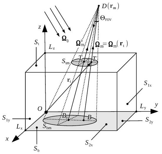
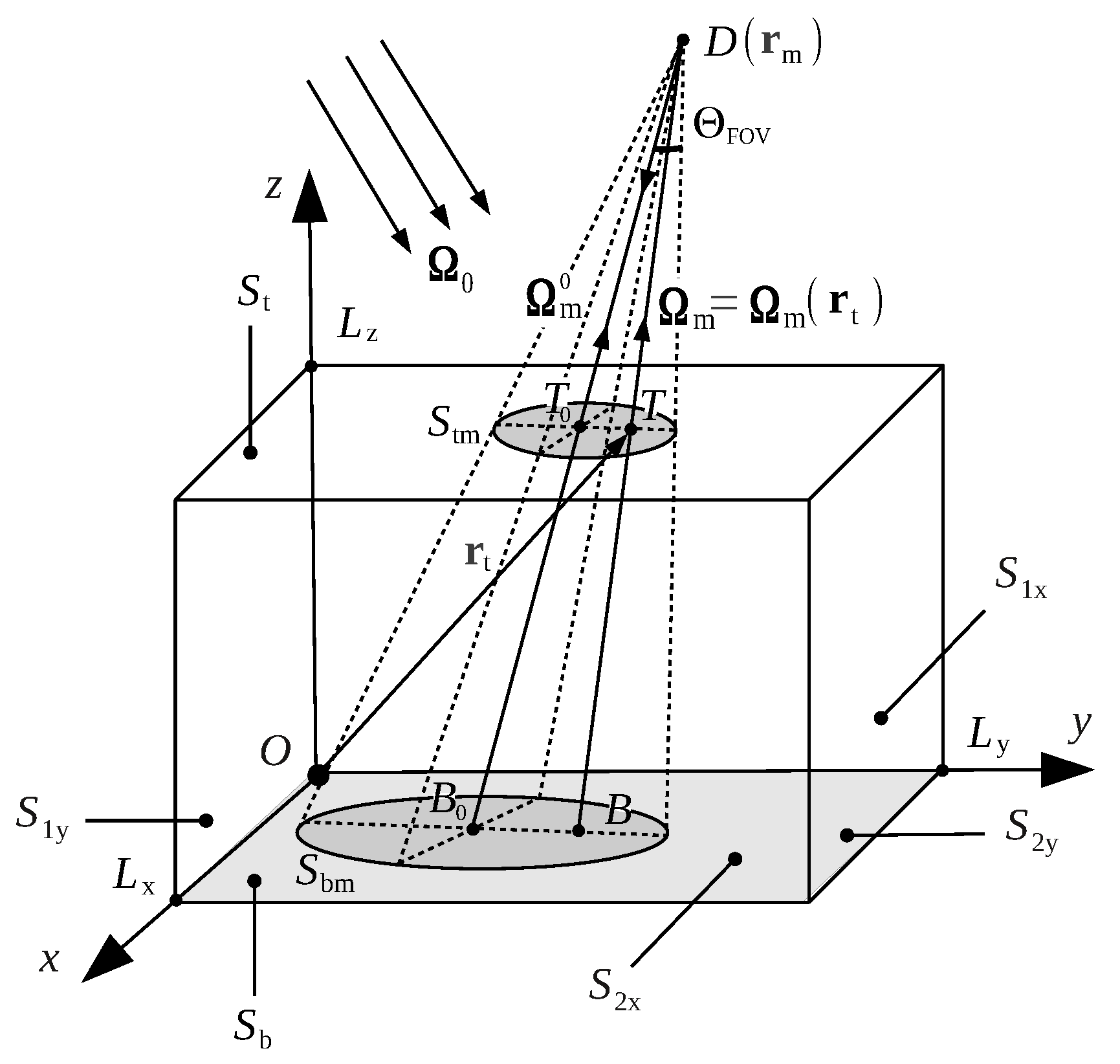
Let us consider the solar radiative transfer in a rectangular prism of lengths $L_{\mathrm{x}}$, $L_{\mathrm{y}}$ and $L_{\mathrm{z}}$ as shown in Figure 1. The top and bottom faces of the prism are denoted by $S_{\mathrm{t}}$ and $S_{\mathrm{b}}$, respectively, while $S_{1\mathrm{x}}$ ($x=0$), $S_{2\mathrm{x}}$ ($x=L_{\mathrm{x}}$), $S_{1\mathrm{y}}$ ($y=0$), and $S_{2\mathrm{y}}$ ($y=L_{\mathrm{y}}$) correspond to the lateral faces. The boundary-value problem for the total radiance at point $\mathbf{r}$ in direction $\mathbf{\Omega }$ consists of the inhomogeneous differential equation

$$\begin{array}{cc}\hfill & \frac{\mathrm{d}I}{\mathrm{d}s}(\lambda ,\mathbf{r},\mathbf{\Omega })=-{\sigma }_{\mathrm{ext}}(\lambda ,\mathbf{r})I(\lambda ,\mathbf{r},\mathbf{\Omega })+\frac{{\sigma }_{\mathrm{sct}}(\lambda ,\mathbf{r})}{4\pi }{\int }_{\mathbf{\Omega }}P(\lambda ,\mathbf{r},\mathbf{\Omega },{\mathbf{\Omega }}^{\prime })I(\lambda ,\mathbf{r},{\mathbf{\Omega }}^{\prime })\mathrm{d}{\mathbf{\Omega }}^{\prime },\hfill \end{array}$$

(1)

the top-of-atmosphere boundary condition

$$I(\lambda ,{\mathbf{r}}_{\mathrm{t}},{\mathbf{\Omega }}^{-})=\frac{F_0(\lambda )}{{\mu }_0}\delta ({\mathbf{\Omega }}^{-}-{\mathbf{\Omega }}_0),{\mathbf{r}}_{\mathrm{t}}\in S_{\mathrm{t}},$$

(2)

and the Lambertian surface boundary condition

$$\begin{array}{cc}\hfill I(\lambda ,{\mathbf{r}}_{\mathrm{b}},{\mathbf{\Omega }}^{+})& =\frac{A(\lambda )}{\pi }{\int }_{{\mathbf{\Omega }}^{-}}I(\lambda ,{\mathbf{r}}_{\mathrm{b}},{\mathbf{\Omega }}^{-})\left|{\mu }^{-}\right|\mathrm{d}{\mathbf{\Omega }}^{-},{\mathbf{r}}_{\mathrm{b}}\in S_{\mathrm{b}}.\hfill \end{array}$$

(3)

Figure 1. Scheme of the radiative transfer problem.

At the horizontal boundaries, periodic boundary conditions are assumed, i.e.,

$$I(\lambda ,{\mathbf{r}}_{1\mathrm{x}},\mathbf{\Omega })=I(\lambda ,{\mathbf{r}}_{2\mathrm{x}},\mathbf{\Omega }),I(\lambda ,{\mathbf{r}}_{1\mathrm{y}},\mathbf{\Omega })=I(\lambda ,{\mathbf{r}}_{2\mathrm{y}},\mathbf{\Omega }),$$

(4)

for ${\mathbf{r}}_{i\mathrm{x}}\in S_{i\mathrm{x}}$ and ${\mathbf{r}}_{i\mathrm{y}}\in S_{i\mathrm{y}}$ with $i=1,2$. In Equations (1)–(4), $\lambda$ is the wavelength, ${\sigma }_{\mathrm{ext}}(\lambda ,\mathbf{r})$ and ${\sigma }_{\mathrm{sct}}(\lambda ,\mathbf{r})$ the extinction and scattering coefficients, respectively, $P(\lambda ,·)$ the phase function, $A(\lambda )$ the surface albedo, ${\mathbf{\Omega }}_0=(-{\mu }_0,{\phi }_0)$ with ${\mu }_0>0$, the solar direction, $F_0(\lambda )$ the solar flux, ${\mathbf{r}}_{2\mathrm{x}}={\mathbf{r}}_{1\mathrm{x}}+L_{\mathrm{x}}\mathbf{i}$ and ${\mathbf{r}}_{2\mathrm{y}}={\mathbf{r}}_{1\mathrm{y}}+L_{\mathrm{y}}\mathbf{j}$ with $(\mathbf{i},\mathbf{j},\mathbf{k})$ being the Cartesian unit vectors. Moreover, ${\mathbf{\Omega }}^{+}$ and ${\mathbf{\Omega }}^{-}$ stand for an upward and a downward direction, respectively, $\Omega$ is the unit sphere, while ${\Omega }^{+}$ and ${\Omega }^{-}$ denote the upper and lower unit hemispheres, respectively,

An instrument placed at point ${\mathbf{r}}_{\mathrm{m}}$ measures the radiance at the top of the atmosphere in direction ${\mathbf{\Omega }}_{\mathrm{m}}^0=({\mu }_{\mathrm{m}}^0,{\phi }_{\mathrm{m}}^0)$, ${\mu }_{\mathrm{m}}^0>0$. Denoting by $g(\lambda )$ the slit function of the instrument, s the slit width, and $S_{\mathrm{tm}}$ the footprint of the instrument on the top face $S_{\mathrm{t}}$, the spectral signal measured by the instrument at wavelength ${\lambda }_{\mathrm{m}}$ in the spectral interval $[{\lambda }_{\min },{\lambda }_{\max }]$ is given by

$$\begin{array}{cc}\hfill \mathcal{I}({\lambda }_{\mathrm{m}})& ={\int }_{{\lambda }_{\min }-s/2}^{{\lambda }_{\max }+s/2}g({\lambda }_{\mathrm{m}}-{\lambda }^{\prime }){\mathcal{I}}_{\mathrm{FOV}}({\lambda }^{\prime })\mathrm{d}{\lambda }^{\prime },\hfill \end{array}$$

(5)

where

$${\mathcal{I}}_{\mathrm{FOV}}({\lambda }^{\prime })={\int }_{S_{\mathrm{t}}}h({\mathbf{r}}_{\mathrm{t}})I({\lambda }^{\prime },{\mathbf{r}}_{\mathrm{t}},{\mathbf{\Omega }}_{\mathrm{m}}({\mathbf{r}}_{\mathrm{t}}))\mathrm{d}{S}_{\mathrm{t}},$$

(6)

is the signal integrated over the field of view of the instrument at wavelength ${\lambda }^{\prime }$, ${\mathbf{\Omega }}_{\mathrm{m}}({\mathbf{r}}_{\mathrm{t}})$ the unit vector along the line connecting the points ${\mathbf{r}}_{\mathrm{t}}\in S_{\mathrm{tm}}$ and ${\mathbf{r}}_{\mathrm{m}}$, i.e., ${\mathbf{\Omega }}_{\mathrm{m}}({\mathbf{r}}_{\mathrm{t}})=({\mathbf{r}}_{\mathrm{m}}-{\mathbf{r}}_{\mathrm{t}})/|{\mathbf{r}}_{\mathrm{m}}-{\mathbf{r}}_{\mathrm{t}}|$ (see Figure 1), and

$$h({\mathbf{r}}_{\mathrm{t}})=\left\{\begin{array}{c}{\displaystyle \frac{1}{A_{\mathrm{tm}}}},{\mathbf{r}}_{\mathrm{t}}\in S_{\mathrm{tm}}\hfill \\ \\ 0,\mathrm{otherwise}\hfill \end{array}\right.,$$

(7)

and $A_{\mathrm{tm}}$ the characteristic function and the area of the instrument footprint, respectively. Assuming that the distance from the top of the atmosphere to the instrument is large, we approximate $I({\lambda }^{\prime },\mathbf{r},{\mathbf{\Omega }}_{\mathrm{m}}(\mathbf{r}))\approx I({\lambda }^{\prime },\mathbf{r},{\mathbf{\Omega }}_{\mathrm{m}}^0)$ in Equation (6).

For an atmosphere consisting of gas molecules and a cloud, we suppose that

• the optical coefficients of the gas molecules depend on the altitude level and the wavelength, and
• the optical coefficients of the cloud depend on the spatial coordinates but not on the wavelength.

The extinction coefficient is then computed as

$${\sigma }_{\mathrm{ext}}(\lambda ,\mathbf{r})={\sigma }_{\mathrm{ext}}^{\mathrm{cloud}}(\mathbf{r})+{\sigma }_{\mathrm{sct}}^{\mathrm{mol}}(\lambda ,z)+{\sigma }_{\mathrm{abs}}^{\mathrm{gas}}(\lambda ,z),$$

(8)

where ${\sigma }_{\mathrm{ext}}^{\mathrm{cloud}}(\mathbf{r})$ is the extinction coefficient in the cloud, ${\sigma }_{\mathrm{sct}}^{\mathrm{mol}}(\lambda ,z)$ the molecular scattering coefficient due to Rayleigh scattering, ${\sigma }_{\mathrm{abs}}^{\mathrm{gas}}(\lambda ,z)$ the gas absorption coefficient, and $(x,y,z)$ the Cartesian coordinates of point $\mathbf{r}$. For the scattering coefficient, we have a similar representation, namely,

$${\sigma }_{\mathrm{sct}}(\lambda ,\mathbf{r})={\omega }_{\mathrm{cloud}}{\sigma }_{\mathrm{ext}}^{\mathrm{cloud}}(\mathbf{r})+{\sigma }_{\mathrm{sct}}^{\mathrm{mol}}(\lambda ,z),$$

(9)

where ${\omega }_{\mathrm{cloud}}$ is the single-scattering albedo of the cloud.

The goal of our analysis is to design an approach for accelerating the computation of the spectral signal $\mathcal{I}({\lambda }_{\mathrm{m}})$ at a set of $W_{\mathrm{m}}$ spectral points ${\left\{{\lambda }_{\mathrm{m}w}\right\}}_{w=1}^{W_{\mathrm{m}}}$ characterizing the instrument. For this purpose, we combine the correlated k-distribution method with some dimensionality reduction techniques.

2.1. Correlated k-Distribution Method

The correlated k-distribution method [4,12] is based on grouping spectral intervals according to absorption coefficient strength. In this section we provide a description of the correlated k-distribution method, which will enable us to connect this method with dimensionality reduction techniques.

Let ${\left\{{\overline{\lambda }}_k\right\}}_{k=1}^{\overline{W}}$ be a discrete set of $\overline{W}$ equally spaced wavelengths in the interval $[{\lambda }_{\min }-s/2,{\lambda }_{\max }+s/2]$ with

$${\overline{\lambda }}_1-\frac{\Delta \lambda }{2}={\lambda }_{\min }-\frac{s}{2}\mathrm{and}{\lambda }_{\overline{W}}+\frac{\Delta \lambda }{2}={\lambda }_{\max }+\frac{s}{2},$$

where $\Delta \lambda$ the discretization step. The forward-model spectral set ${\left\{{\overline{\lambda }}_k\right\}}_{k=1}^{\overline{W}}$ is finer than the measurement spectral set ${\left\{{\lambda }_{\mathrm{m}w}\right\}}_{w=1}^{W_{\mathrm{m}}}$; in practice, $\overline{W}$ is chosen as a multiple of $W_{\mathrm{m}}$, i.e., $\overline{W}=c{W}_{\mathrm{m}}$ with say, c being an integer greater than $20.$ The convolution integral giving the expression of the spectral signal measured by the instrument can be approximated by

$$\begin{array}{cc}\hfill & \mathcal{I}({\lambda }_{\mathrm{m}})={\int }_{{\lambda }_{\min }-s/2}^{{\lambda }_{\max }+s/2}g({\lambda }_{\mathrm{m}}-{\lambda }^{\prime }){\mathcal{I}}_{\mathrm{FOV}}({\lambda }^{\prime })\mathrm{d}{\lambda }^{\prime }\approx \sum _{k=1}^{\overline{W}}g({\lambda }_{\mathrm{m}}-{\overline{\lambda }}_k){\int }_{{\overline{\lambda }}_k-\Delta \lambda /2}^{{\overline{\lambda }}_k+\Delta \lambda /2}{\mathcal{I}}_{\mathrm{FOV}}({\lambda }^{\prime })\mathrm{d}{\lambda }^{\prime }.\hfill \end{array}$$

(10)

As gas absorption has stronger spectral variation than molecular and particulate scattering, we write formally (at a given altitude level z) ${\mathcal{I}}_{\mathrm{FOV}}(\lambda )={\mathcal{I}}_{\mathrm{FOV}}({\sigma }_{\mathrm{abs}}^{\mathrm{gas}}(\lambda ))$. The accurate technique for computing the integral in Equation (10) is a line-by-line (LBL) calculation of the gas absorption coefficient versus wavelength. Contrarily, the correlated k-distribution method is based on the fact that for a homogeneous atmosphere, the transmission within a spectral interval is independent of the LBL variation of ${\sigma }_{\mathrm{abs}}^{\mathrm{gas}}$ with respect to the wavelength, but rather depends only on the distribution of ${\sigma }_{\mathrm{abs}}^{\mathrm{gas}}$ within the spectral interval [13]. In this regard, let $F=F({\sigma }_{\mathrm{abs},k}^{\mathrm{gas}})$ be the cumulative density function of ${\sigma }_{\mathrm{abs}}^{\mathrm{gas}}(\lambda )$ in the spectral interval $[{\overline{\lambda }}_k-\Delta \lambda /2,{\overline{\lambda }}_k+\Delta \lambda /2]$, and ${\sigma }_{\mathrm{abs},k}^{\mathrm{gas}}(F)$ the quantile function (i.e., the inverse function of the cumulative distribution function). The spectral signal measured by the instrument can then be computed as

$$\begin{array}{cc}\hfill & \mathcal{I}({\lambda }_{\mathrm{m}})=\Delta \lambda \sum _{k=1}^{\overline{W}}g({\lambda }_{\mathrm{m}}-{\overline{\lambda }}_k){\int }_0^1{\mathcal{I}}_{\mathrm{FOV}}({\sigma }_{\mathrm{abs},k}^{\mathrm{gas}}(F))\mathrm{d}F=\Delta \lambda \sum _{k=1}^{\overline{W}}g({\lambda }_{\mathrm{m}}-{\overline{\lambda }}_k)\sum _{l=1}^{N_{\mathrm{q}}}{\varpi }_l{\mathcal{I}}_{\mathrm{FOV}}({\sigma }_{\mathrm{abs},k}^{\mathrm{gas}}(F_l)),\hfill \end{array}$$

(11)

where ${\{F_l,{\varpi }_l\}}_{l=1}^{N_{\mathrm{q}}}$ is a set of $N_{\mathrm{q}}$ quadrature points and weights in the interval $[0,1]$. The ${\sigma }_{\mathrm{abs},k}^{\mathrm{gas}}(F_l)$ can be computed by inverting the cumulative density functions of the LBL gas absorption coefficients, or in the case of the “exponential sum fitting of transmittance” method [14], by solving a nonlinear least squares problem.

In the final step, we define the sets of wavelengths and weights ${\left\{{\lambda }_w\right\}}_{w=1}^W$ and ${\left\{{\omega }_w\right\}}_{w=1}^W$ with $W=\overline{W}{N}_{\mathrm{q}}$, respectively, through the relations ${\lambda }_w={\overline{\lambda }}_k$ and ${\omega }_w=\Delta \lambda {\varpi }_l$, where $w=l+(k-1)N_{\mathrm{q}}$ for $k=1,\dots ,\overline{W},l=1,\dots ,N_{\mathrm{q}}$. Accordingly, we set ${\sigma }_{\mathrm{abs}}^{\mathrm{gas}}({\lambda }_w)={\sigma }_{\mathrm{abs},k}^{\mathrm{gas}}(F_l)$. Note that ${\left\{{\lambda }_w\right\}}_{w=1}^W$ contains $\overline{W}$ groups of $N_{\mathrm{q}}$ identical wavelengths. By this construction, Equation (11) becomes

$$\mathcal{I}({\lambda }_{\mathrm{m}})=\sum _{w=1}^W{\omega }_{w}g({\lambda }_{\mathrm{m}}-{\lambda }_w){\mathcal{I}}_{\mathrm{FOV}}({\sigma }_{\mathrm{abs}}^{\mathrm{gas}}({\lambda }_w)).$$

(12)

Note that Equation (12) is a quadrature rule for the convolution integral (10) in the case of the correlated k-distribution method.

The computation of the spectral signal by means of the correlated k-distribution method requires the computation of the absorption coefficients ${\sigma }_{\mathrm{abs}}^{\mathrm{gas}}({\lambda }_w,z)$ at the set of wavelengths ${\left\{{\lambda }_w\right\}}_{w=1}^W$, and so, W monochromatic radiative transfer calculations. For applications with $c\ge 20$ and $N_{\mathrm{q}}\ge 4$, $W=\overline{W}{N}_{\mathrm{q}}=c{W}_{\mathrm{m}}{N}_{\mathrm{q}}$ can be in the order of hundreds, and a further acceleration is needed. This can be achieved by applying dimensionality reduction techniques on the optical parameters.

2.2. Dimensionality Reduction of Atmospheric Optical Parameters

Following Ref. [11], the dimensionality reduction problem of the optical parameters can be formulated as follows. For each wavelength ${\lambda }_w$, we define an N-dimensional vector ${\mathbf{x}}_w$ by

$${\mathbf{x}}_w^T=\left[ln{\sigma }_{\mathrm{abs},1}^{\mathrm{gas}}({\lambda }_w),\dots ,ln{\sigma }_{\mathrm{abs},L}^{\mathrm{gas}}({\lambda }_w),ln{\sigma }_{\mathrm{sct},1}^{\mathrm{mol}}({\lambda }_w),\dots ,ln{\sigma }_{\mathrm{sct},L}^{\mathrm{mol}}({\lambda }_w),ln{F}_0({\lambda }_w)\right],$$

(13)

where ${\sigma }_{\mathrm{abs},k}^{\mathrm{gas}}$ and ${\sigma }_{\mathrm{sct},k}^{\mathrm{mol}}$ are the optical coefficients in the kth level, $N=2N_{\mathrm{z}}+1$, and $N_{\mathrm{z}}$ is the number of altitude levels. For simplicity, the surface albedo A was not included in ${\mathbf{x}}_w$ (we assumed that the variations of A are negligible over the width of a molecular absorption band). Thus, the wavelength variability of the optical parameters is encapsulated in the vector ${\mathbf{x}}_w\in {\mathbb{R}}^N$, and there is a one-to-one correspondence between the discrete set of wavelengths ${\left\{{\lambda }_w\right\}}_{w=1}^W$, and the discrete set of optical parameters ${\left\{{\mathbf{x}}_w\right\}}_{w=1}^W$. For the N-dimensional data set ${\left\{{\mathbf{x}}_w\right\}}_{w=1}^W$, $\overline{\mathbf{x}}=(1/W){\sum }_{w=1}^W{\mathbf{x}}_w$ is the sample mean of the data. The goal of a dimensionality reduction technique is to find an M-dimensional subspace ($M<N$) spanned by a set of linear independent vectors ${\left\{{\mathbf{a}}_k\right\}}_{k=1}^M$, such that the centered data ${\mathbf{x}}_w-\overline{\mathbf{x}}$ belong to this subspace; that is,

$${\mathbf{x}}_w\approx \overline{\mathbf{x}}+\sum _{k=1}^M{y}_{wk}{\mathbf{a}}_k=\overline{\mathbf{x}}+\mathbf{A}{\mathbf{y}}_w,w=1,\dots ,W.$$

(14)

In Equation (14), the matrix $\mathbf{A}={\left[{\mathbf{a}}_k\right]}_{k=1}^M\in {\mathbb{R}}^{N\times M}$, encapsulating the column vectors ${\mathbf{a}}_k$, represents the inverse transform from the low-dimensional space to the high-dimensional space, and $y_{wk}$ is the kth component of ${\mathbf{y}}_w\in {\mathbb{R}}^M$. The vector ${\mathbf{y}}_w$ is given by the forward transform from the high-dimensional space to the low-dimensional space,

$${\mathbf{y}}_w={\mathbf{A}}^{†}({\mathbf{x}}_w-\overline{\mathbf{x}}),$$

(15)

where ${\mathbf{A}}^{†}={({\mathbf{A}}^T\mathbf{A})}^{-1}{\mathbf{A}}^T\in {\mathbb{R}}^{M\times N}$ is the pseudoinverse of $\mathbf{A}$.

An approximate model for estimating the integrated signal of the instrument at wavelength $\lambda$ is of the form

$$ln\frac{{\mathcal{I}}_{\mathrm{FOV}}(\lambda )}{{\mathcal{I}}_{\mathrm{FOV}}^{\mathrm{a}}(\lambda )}=f(\lambda ),$$

(16)

where ${\mathcal{I}}_{\mathrm{FOV}}^{\mathrm{a}}(\lambda )$ is the integrated signal computed by an approximate radiative transfer model, and $f(\lambda )$ a correction factor. The correction factor $f(\lambda )$ can be calculated efficiently and accurately by means of dimensionality reduction techniques applied on the optical parameters. Let us assume that the scalar function $f({\mathbf{x}}_w)$ given by Equation (16) is not too nonlinear in ${\mathbf{x}}_w$. The computational process is organized as follows.

• For (cf. Equation (14))

  $$\Delta {\mathbf{x}}_w={\mathbf{x}}_w-\overline{\mathbf{x}}=\sum _{k=1}^M{y}_{wk}{\mathbf{a}}_k=\mathbf{A}{\mathbf{y}}_w,$$

  (17)
  $f({\mathbf{x}}_w)$ is approximated by a second-order Taylor expansion around $\overline{\mathbf{x}}$; that is,

  $$f({\mathbf{x}}_w)\approx f(\overline{\mathbf{x}}+\Delta {\mathbf{x}}_w)\approx f(\overline{\mathbf{x}})+\Delta {\mathbf{x}}_w^T\nabla f(\overline{\mathbf{x}})+\frac{1}{2}\Delta {\mathbf{x}}_w^T{\nabla }^{2}f(\overline{\mathbf{x}})\Delta {\mathbf{x}}_w,$$

  (18)

  where $\nabla f$ and ${\nabla }^{2}f$ are the gradient and the Hessian of f, respectively.
• For ${\mathbf{a}}_k=\left|\right|{\mathbf{a}}_k\left|\right|{\widehat{\mathbf{a}}}_k$ and in view of Equation (17), the second and third terms in Equation (18) are written as

  $$\Delta {\mathbf{x}}_w^T\nabla f(\overline{\mathbf{x}})=\sum _{k=1}^M{y}_{wk}\left|\right|{\mathbf{a}}_k\left|\right|\frac{\partial f}{\partial {\widehat{a}}_k}(\overline{\mathbf{x}})$$

  (19)

  and

  $$\Delta {\mathbf{x}}_w^T{\nabla }^{2}f(\overline{\mathbf{x}})\Delta {\mathbf{x}}_w=\sum _{k=1}^M\sum _{l=1}^M{y}_{wk}{y}_{wl}\left|\right|{\mathbf{a}}_k\left|\right|\left|\right|{\mathbf{a}}_l\left|\right|\frac{{\partial }^{2}f}{\partial {\widehat{a}}_k\partial {\widehat{a}}_l}(\overline{\mathbf{x}}),$$

  (20)

  respectively.
• The mixed directional derivatives in Equation (20) are neglected, while the first- and second-order directional derivatives are approximated by means of central differences; that is,

  $$\frac{\partial f}{\partial {\widehat{a}}_k}(\overline{\mathbf{x}})\approx \frac{f(\overline{\mathbf{x}}+h{\widehat{\mathbf{a}}}_k)-f(\overline{\mathbf{x}}-h{\widehat{\mathbf{a}}}_k)}{2h},$$

  (21)

  and

  $$\frac{{\partial }^{2}f}{\partial {\widehat{a}}_k^2}(\overline{\mathbf{x}})\approx \frac{f(\overline{\mathbf{x}}+h{\widehat{\mathbf{a}}}_k)-2f(\overline{\mathbf{x}})+f(\overline{\mathbf{x}}-h{\widehat{\mathbf{a}}}_k)}{h^2},$$

  (22)

  respectively.
• For $h=\left|\right|{\mathbf{a}}_k\left|\right|$, Equations (18)–(22) yield the computational formula:

  $$\begin{array}{cc}\hfill & f({\mathbf{x}}_w)\approx f(\overline{\mathbf{x}})+\frac{1}{2}\sum _{k=1}^M[f(\overline{\mathbf{x}}+{\mathbf{a}}_k)-f(\overline{\mathbf{x}}-{\mathbf{a}}_k)]y_{wk}+\frac{1}{2}\sum _{k=1}^M[f(\overline{\mathbf{x}}+{\mathbf{a}}_k)-2f(\overline{\mathbf{x}})+f(\overline{\mathbf{x}}-{\mathbf{a}}_k)]y_{wk}^2.\hfill \end{array}$$

  (23)

From Equation (23), it is apparent that the computation of $f({\mathbf{x}}_w)$ requires $2M+1$ calls of the exact and approximate models, while the computation of ${\mathcal{I}}_{\mathrm{FOV}}({\lambda }_w)$ requires, in addition, W calls of the approximate model. In this regard and taking into account that $M\ll W$, we are led to a substantial reduction of the computational time.

The most widely used dimensionality reduction techniques are the linear embedding methods which are summarized below.

• The principal component analysis (PCA) [15] performs a dimensionality reduction by projecting the original N-dimensional data on the M-dimensional subspace spanned by the dominant singular vectors of the data covariance matrix.
• The locality pursuit embedding (LPE) [16] performs a principal component analysis on local nearest neighbor patches to reveal the tangent space structure on the M-dimensional subspace.
• The locality preserving projection (LPP) [17] solves a variational problem that optimally preserves the neighborhood structure of the data set.
• The locally embedded analysis (LEA) [18] uses an embedding strategy based on a linear eigenspace analysis to minimize the local reconstruction error.

It should be pointed out that PCA preserves only the global structure of the data, and may fail to preserve the local structure if the data lie on a nonlinear manifold. In contrast, LPE, LPP, and LEA are local linear approaches, which optimally preserve local neighborhood information (the local structure of the data) in a certain sense.

The PCA, LPE, LPP, and LEA methods are illustrated in Algorithms A1–A4 of Appendix A. The outputs of these algorithms are the linear mapping $\mathbf{A}$ and the vectors of parameters ${\mathbf{y}}_w$, $w=1,\dots ,W$. Note that in the PCA language, the column vectors ${\mathbf{a}}_k$, $k=1,\dots ,M$ of $\mathbf{A}$ are the so-called empirical orthogonal functions, while the vectors of parameters ${\mathbf{y}}_w$, $w=1,\dots ,W$ are the principal components.

A last problem which has to be solved is the choice of an approximate model. Two special features of SHDOM facilitate this choice, namely, the use (i) of spherical harmonics and discrete ordinates to represent the radiance field, and (ii) of a sort of successive order of scattering solution method (Picard iteration). In a first approximate model, we choose 2 zenith discrete angles per hemisphere to represent the radiance field; analogous to the one-dimensional radiative transfer, the resulting method is called the four-stream approximation. In a second approximate model, we consider only 2 steps of the method of Picard iteration; the resulting method is called the second-order of scattering approximation.

In summary, the spectral acceleration approach includes two steps. The first step is a pre-processing step, consisting in the computation of the sets of wavelengths ${\left\{{\lambda }_w\right\}}_{w=1}^W$, the absorption coefficients ${\sigma }_{\mathrm{abs}}^{\mathrm{gas}}({\lambda }_w,z)$, and the weighting factors ${\left\{{\omega }_w\right\}}_{w=1}^W$ in the framework of the correlated k-distribution method. The second step is a computational step, consisting of the calculation of

• the data vectors ${\mathbf{x}}_w$, $w=1,\dots ,W$, the empirical orthogonal functions ${\mathbf{a}}_k$, $k=1,\dots ,M$, and the principal components ${\mathbf{y}}_w$, $w=1,\dots ,W$ in the framework of dimensionality reduction techniques,
• the correction factor $f({\mathbf{x}}_w)$, $w=1,\dots ,W$, and the integrated signal ${\mathcal{I}}_{\mathrm{FOV}}({\lambda }_w)$, $w=1,\dots ,W$ according to Equations (23) and (16), respectively, and finally,
• the spectral signal measured by the instrument $\mathcal{I}({\lambda }_{\mathrm{mw}})$, $w=1,\dots ,W_{\mathrm{m}}$ by means of Equation (10).

3. Numerical Analysis

Before presenting some numerical results, we describe an implementation of SHDOM that is devoted to the retrieval of atmospheric trace gas concentrations from space-borne spectral measurements of radiation reflected through the Earth’s atmosphere.

3.1. SHDOM Implementation

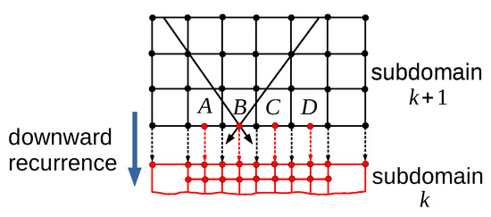
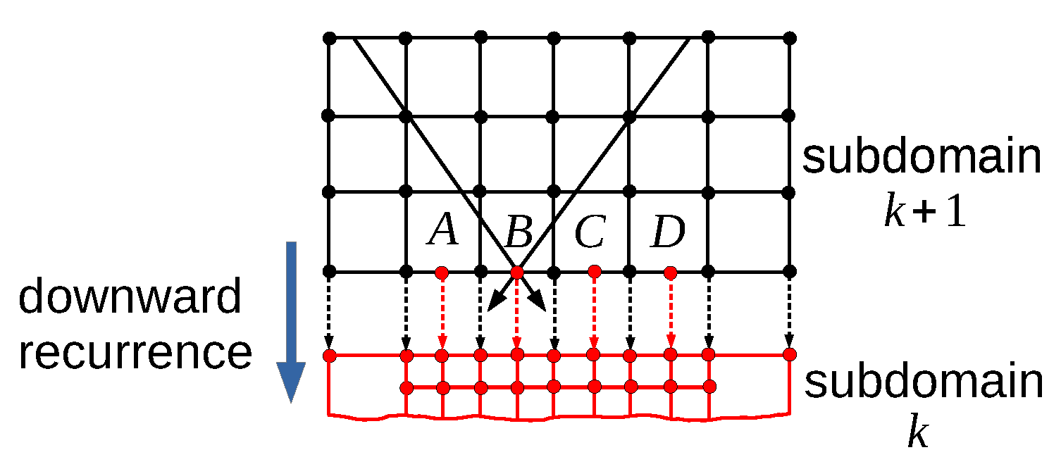
For an atmosphere consisting of gas molecules, we have to consider a domain of analysis with a large vertical extent, especially when dealing with trace retrievals. The reason is that gas molecules have a vertical concentration profile up to several tens of kilometers. Unfortunately, for large problems, SHDOM is limited by the amount of memory available for calculation, in particular on smaller computers. To handle this problem, in our implementation of SHDOM, we divide the domain of analysis into a number of subdomains along the vertical direction, and for each subdomain, we store the radiance and source function in separate files. The optical properties and the direct solar beam are calculated at each point on the base grid of the entire domain of analysis, while (i) the radiative transfer equation integration along each discrete ordinate during the solution iterations and (ii) the integration along the viewing directions for the intensity output are done successively moving from one subdomain to the neighboring one. Each subdomain has its own grid obtained by the cell splitting (adaptive grid) procedure. At the boundaries of a subdomain, the radiances are calculated not only at the grid points of the subdomain itself, but also at the grid points corresponding to the boundaries of the neighboring subdomains (Figure 2). This is done by integrating the radiative transfer equation and by applying the standard interpolation approach (the entering and exiting values of the extinction and extinction-source function product are computed using bilinear interpolation of the four gridpoint values of the faces pierced by a ray). To ensure the continuity condition for the radiance field, the boundary values of the radiance are passed between the neighboring subdomains. The data are transferred to and from files.

Figure 2. At the lower boundary of the subdomain $k+1$, the downward radiances are also computed at the points A, B, C, and D, which are grid points on the upper boundary of the subdomain k. During the downward iteration step, these boundary values are passed to the subdomain k.

This implementation of SHDOM does not give exactly the same results as the standard implementation because of (i) the splitting decision for the cells situated at the boundaries of a subdomain, and (ii) the differences between the rays along which the radiative transfer equation is integrated (a ray is traced backward until the transmission falls below some minimum specified value only inside a subdomain). However, as compared to the overall accuracy of the algorithm, these errors are small. On the other hand, this implementation increases the computation time by the times which are needed (i) to write and read data to and from files, and (ii) to compute the radiances at the additional grid points on the boundaries of each subdomain. It should be pointed out that the number of subdomains is set by the user and depends on the problem to be solved.

The code can be reformulated as a parallel code by using the Message Passing Interface (MPI). In this context, it should be pointed out that a parallel implementation of SHDOM, but in which the domain of analysis is divided along the horizontal directions, has been described in Ref. [19]. However, in the case of horizontal splitting, the transfer of data between different neighboring subdomains is more challenging for the implementation.

3.2. Numerical Results

The computational domain is a rectangular prism of lengths $L_{\mathrm{x}}=L_{\mathrm{y}}=15$ km and $L_{\mathrm{z}}=40$ km. The discretization steps along the horizontal directions are $\Delta x=\Delta y=0.5$ km; thus, the corresponding numbers of base grid points are $N_{\mathrm{x}}=N_{\mathrm{y}}=30$. Along the vertical direction, the domain is discretized into 8 subdomains; the corresponding altitude levels and discretization steps are listed in Table 1. The cloud is homogeneous in the vertical direction and is placed between 3 and 4 km (second subdomain). The cloud extinction field is modeled as

$${\sigma }_{\mathrm{ext}}^{\mathrm{cloud}}(x,y)={\sigma }_{0}f(x,y),$$

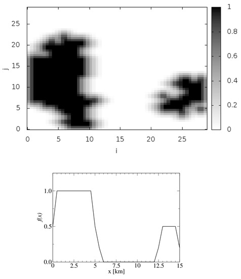
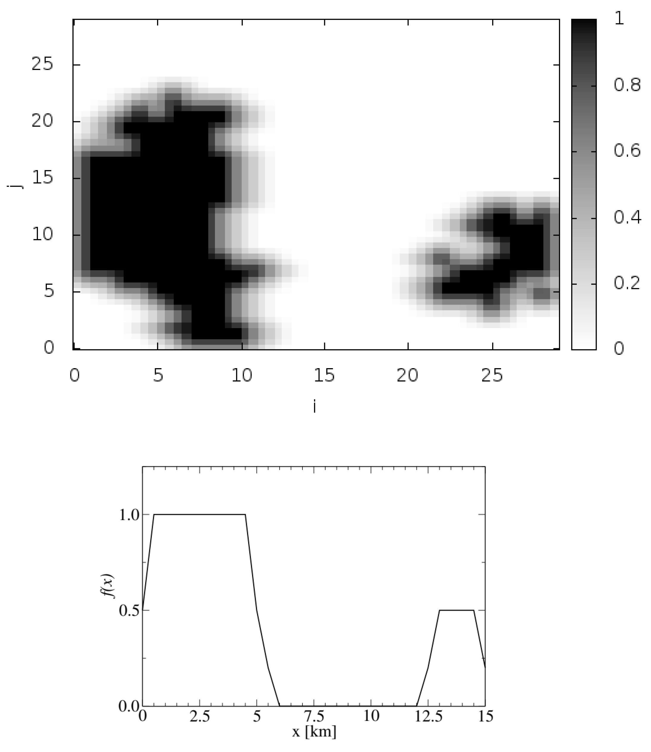
where ${\sigma }_0=6{\mathrm{km}}^{-1}$ and $f(x,y)$ is the indicator function taking the values $f(x,y)=1$ inside the cloud and $f(x,y)=0$ inside the clear sky region. The indicator function $f(x,y)$ is generated by a two-dimensional broken cloud model [20] with a cloud fraction of about $0.4.$ In order to avoid abrupt changes of the extinction field in the horizontal plane, ${\sigma }_{\mathrm{ext}}^{\mathrm{cloud}}(x,y)$ is smoothed at the boundary of a cloudy region (by linear interpolation along two discretization steps in each direction). To simplify the analysis, a Henyey–Greenstein phase function with an asymmetry parameter $g=0.8$ is considered, while the single-scattering albedo is chosen as ${\omega }_{\mathrm{cloud}}=0.99$. The number of discrete zenith and azimuth angles are $N_{\mu }=16$ and $N_{\phi }=2N_{\mu }$, respectively, the solar and instrument zenith angles are ${\theta }_0={60}^{\circ }$ and ${\theta }_{\mathrm{m}}^0={30}^{\circ }$, respectively, the relative azimuth angle is $\Delta \phi =0$, and a Lambertian reflecting surface with the surface albedo $A=0.2$ is assumed. The footprint of the detector is considered to be a square of length $2a=10\Delta x$ centered at $x_0=y_0=L_{\mathrm{x}}/2$, and $z_0=L_{\mathrm{z}}$. The calculations are performed for a mid-latitude summer atmosphere [21] and a wavelength-dependent slit function corresponding to the TROPOspheric Monitoring Instrument (TROPOMI).

Table 1. Discretization of the domain of analysis along the vertical direction.

Subdomain	1	2	3	4	5	6	7	8
Altitude levels [km]	0–3	3–4	4–7	7–10	10–14	14–22	22–30	30–40
Discretization step [km]	0.5	0.1	0.5	0.5	1.0	2.0	2.0	5

SHDOM is run by using an adaptive grid with a splitting accuracy of ${10}^{-4}$. The solution accuracy is ${10}^{-4}$, and the simulations are performed for periodic boundary conditions by using the delta-M approximation along with the untruncated phase function single-scattering solution (TMS correction of Nakajima and Tanaka [22]). The dimensionality reduction parameter M, which determines the approximation accuracy of the linear embedding methods, is chosen as $M=4$. The simulations were performed on a computer Intel Core i5-3340M CPU 2.70GHz with 8 GB RAM.

3.2.1. Oxygen A-Band Test Problem

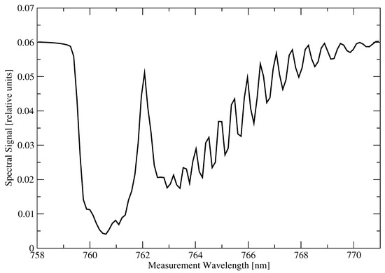
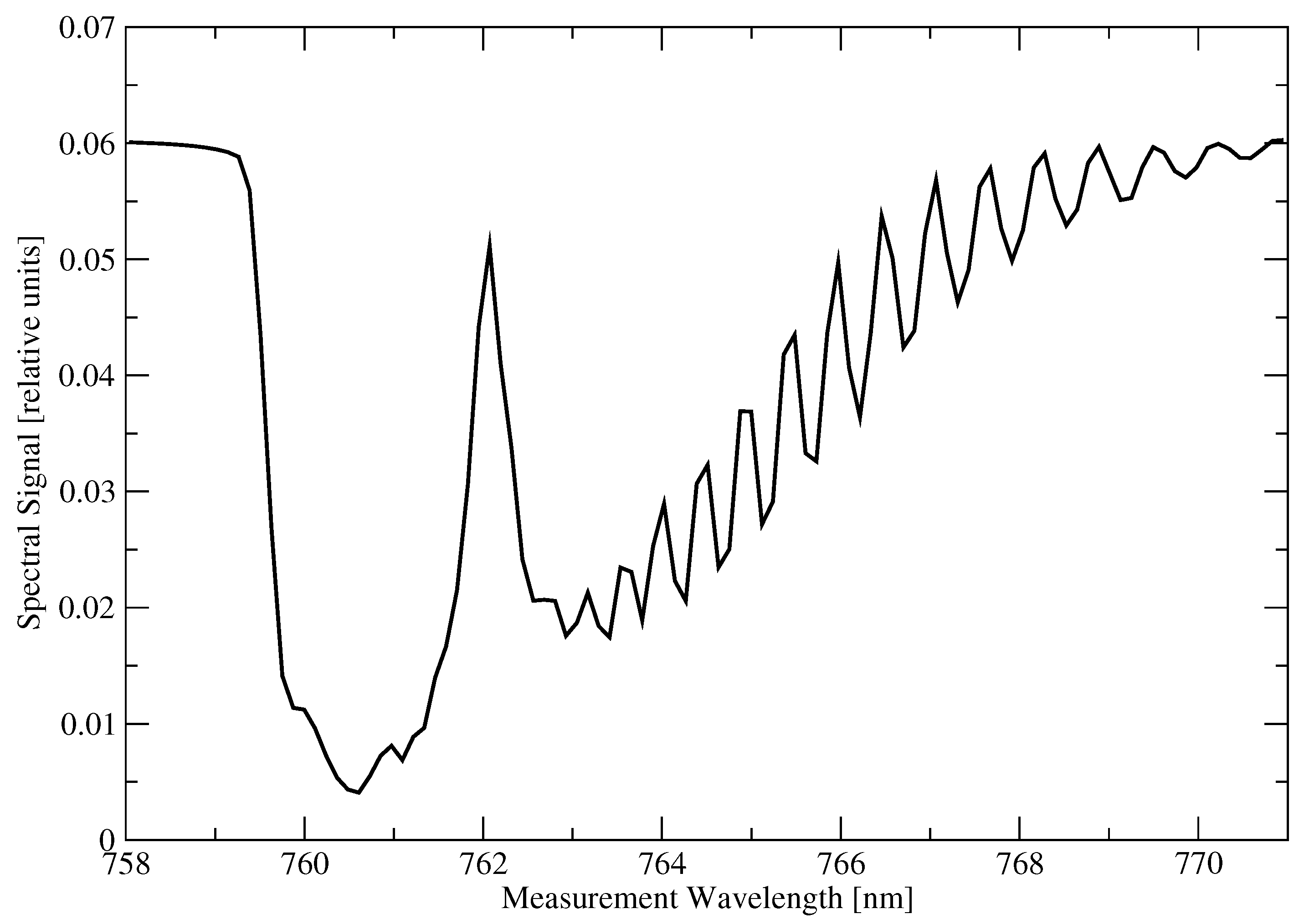
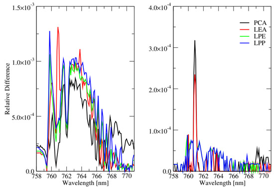
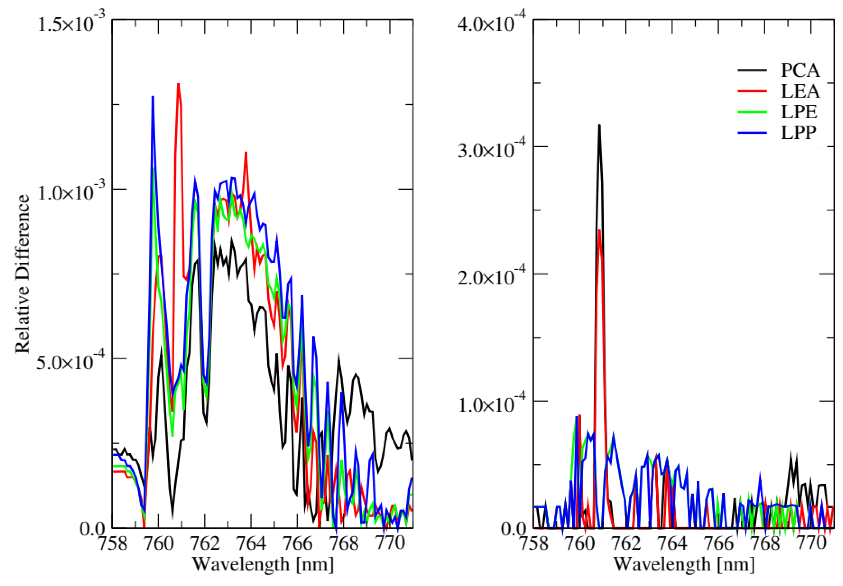
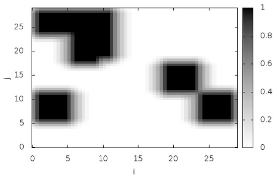
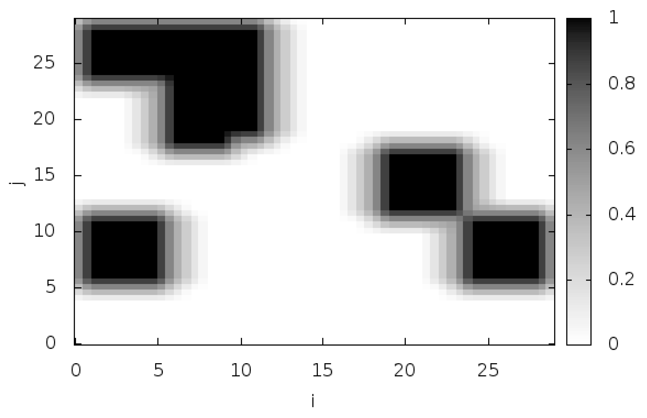
In our first example, we consider, in addition to the scattering and absorption by a cloud, molecular Rayleigh scattering, and the absorption in the Oxygen A-band. The measurement spectral grid contains 107 spectral points between 758 nm and 771 nm, while the number of spectral points for the correlated k-distribution method is $W=936$. For this test, a two-dimensional slice at $y=7$ km is selected from a three-dimensional broken-cloud field (Figure 3). Figure 4 illustrates the spectral signal computed by using SHDOM with the correlated k-distribution method. Using these results as a reference, we show in Figure 5 the relative differences in the spectral signal corresponding to the linear embedding methods, and in Table 2, the RMS of the relative difference and the computational time in hours, minutes, and seconds. The computation time of SHDOM with the correlated k-distribution method was 36 minutes and 28 s. Several conclusions can be formulated:

Figure 3. Upper panel: indicator function $f(x_i,y_j)$ with $x_i=i\Delta x$ and $y_j=j\Delta y$ for the ${\mathrm{O}}_2$A-band test problem. Lower panel: a slice of the indicator function $f(x)$ at $y=7$ km.

Figure 4. Spectral signal for the ${\mathrm{O}}_2$A-band test problem. The differences between SHDOM with the correlated k-distribution method with and without linear embedding methods are not visible in this plot.

Figure 5. Relative differences in the spectral signal for the linear embedding methods and the ${\mathrm{O}}_2$A-band test problem. The plots in the left panel correspond to the four-stream approximation, while the plots in the right panel correspond to the second-order of scattering approximation.

Table 2. Root mean square (RMS) of relative difference and the computational time (CPU) in hours:minutes:seconds corresponding to the linear embedding methods for the ${\mathrm{O}}_2$A-band test problem.

Method		Four-Stream	Second-Order Scattering
PCA	RMS	$6.37\times {10}^{-4}$	$5.19\times {10}^{-5}$
	CPU	0:04:21	0:03:01
LEA	RMS	$5.69\times {10}^{-4}$	$4.00\times {10}^{-5}$
	CPU	0:04:45	0:03:17
LPE	RMS	$5.37\times {10}^{-4}$	$3.29\times {10}^{-5}$
	CPU	0:04:35	0:03:05
LPP	RMS	$6.00\times {10}^{-4}$	$3.14\times {10}^{-5}$
	CPU	0:05:01	0:03:53

• For the dimensionality reduction parameter $M=4$, the relative differences are smaller than $1.25\times {10}^{-3}$ over the entire spectral domain, while the RMS values are smaller than $6.4\times {10}^{-4}$.
• The computation time corresponding to the second-order of scattering approximation is smaller than that corresponding to the four-stream approximation.
• For the second-order of scattering approximation, the fastest linear embedding method is PCA and the most accurate is LPP.
• Relative to the correlated k-distribution method, the acceleration factor is of about 7–12.

3.2.2. ${\mathrm{NO}}_2$-Test Problem

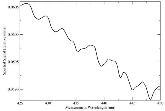
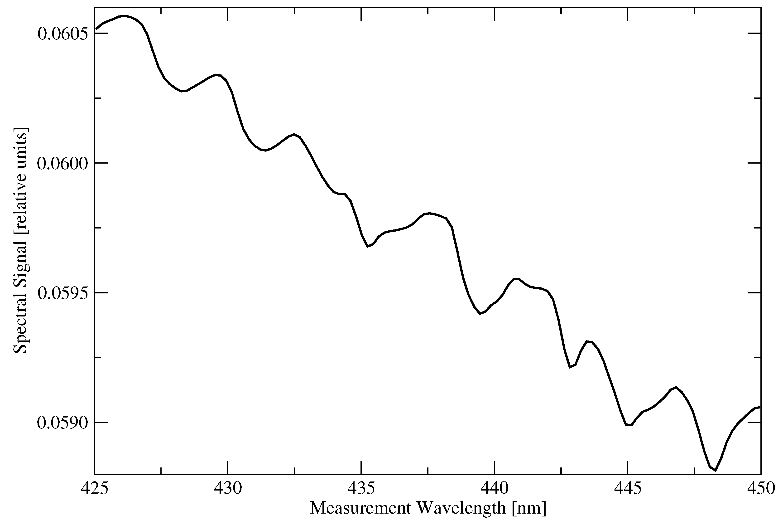
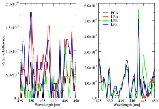
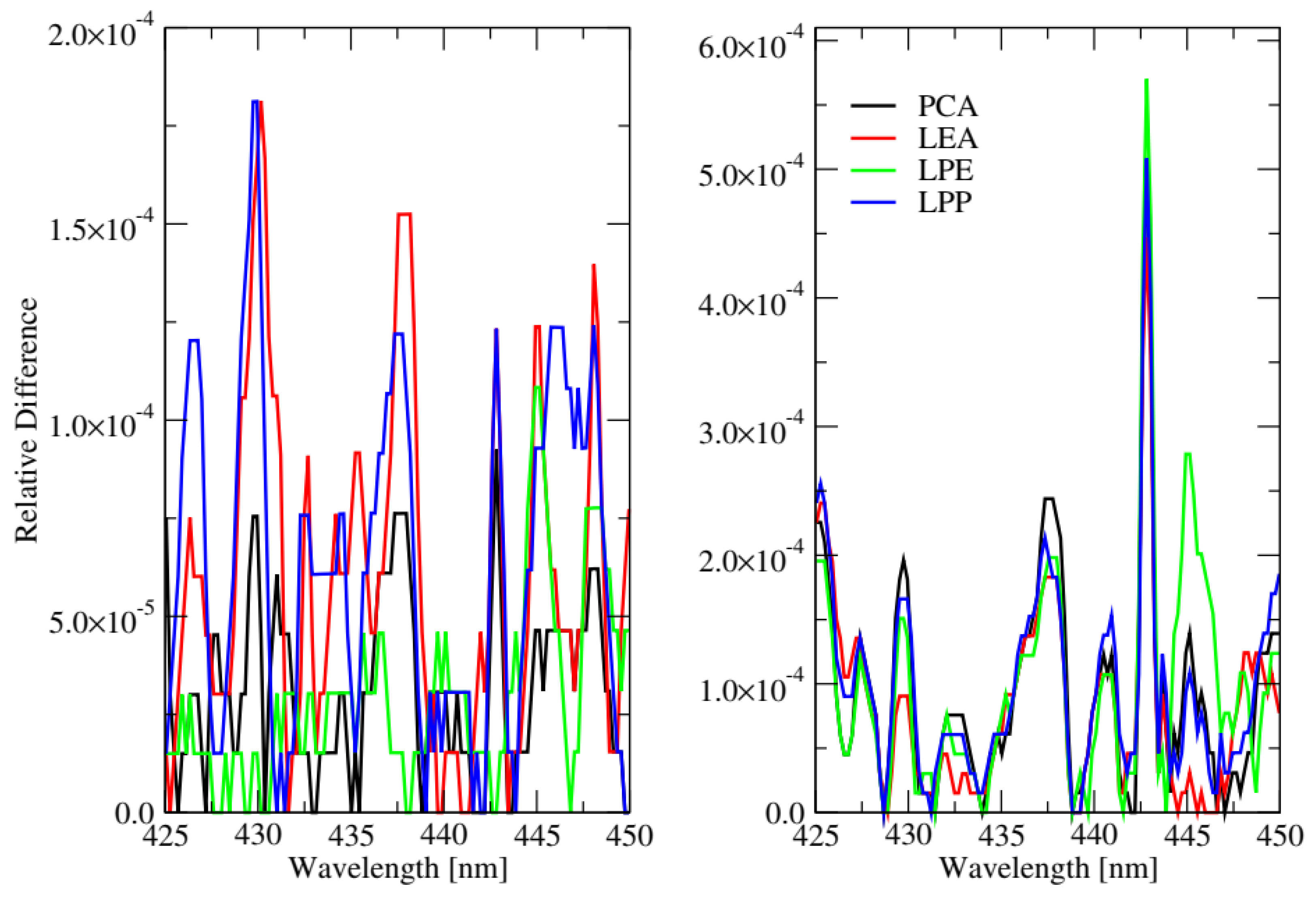
In the second example, the absorption of ${\mathrm{NO}}_2$, ozone (${\mathrm{O}}_3$), oxygen dimer (${\mathrm{O}}_4$), and water vapor is considered. The measurement spectral grid contains 119 spectral points between 425 nm and 450 nm, while the number of spectral points for the correlated k-distribution method is $W=268$. Note that in the correlated k-distribution method, the auxiliary gases are treated as weak absorbers meaning that for these gases, the average values of the LBL cross sections are used in the calculation. The test problem is three-dimensional, and the indicator function of the broken cloud is illustrated in Figure 6. In Table 3, we indicate the amount of memory required for storing the radiance and source function for each subdomain. As a result that the domain of analysis is not excessively large, the total amount of disk memory is 3.168 GB. As a result, we infer that SHDOM can be also run without splitting the domain of analysis. Taking these results as a reference, we found that the relative errors due to the domain splitting procedure are smaller than ${10}^{-3}$. The spectral signal computed by using SHDOM with the correlated k-distribution method is shown in Figure 7, the relative differences in the spectral signal corresponding to the linear embedding methods are plotted in Figure 8, and finally, the RMS of the relative difference and the computational time in hours, minutes, and seconds are given in Table 4. For this test example, the computation time of SHDOM with the correlated k-distribution method was 12 h, 18 min, and 32 s. As in the first test example, we see that

Figure 6. Indicator function $f(x_i,y_j)$ with $x_i=i\Delta x$ and $y_j=j\Delta y$ for the ${\mathrm{NO}}_2$-test problem.

Table 3. Amount of memory required for storing the radiance and source function for each subdomain.

Subdomain	1	2	3	4	5	6	7	8
Memory [MB]	549	924	549	486	228	228	228	52

Figure 7. Spectral signal for the ${\mathrm{NO}}_2$-test problem.

Figure 8. Relative differences in the spectral for the linear embedding methods and the ${\mathrm{NO}}_2$-test problem. The plots in the left panel correspond to the four-stream approximation, while the plots in the right panel correspond to the second-order of scattering approximation.

Table 4. RMS of relative difference and the computational time (CPU) in hours:minutes:seconds corresponding to the linear embedding methods for the ${\mathrm{NO}}_2$-test problem.

Method		Four-Stream	Second-Order Scattering
PCA	RMS	$3.84\times {10}^{-5}$	$1.25\times {10}^{-4}$
	CPU	1:21:24	1:02:56
LEA	RMS	$7.41\times {10}^{-5}$	$1.34\times {10}^{-4}$
	CPU	1:22:18	1:03:48
LPE	RMS	$3.73\times {10}^{-5}$	$1.12\times {10}^{-4}$
	CPU	1:21:53	1:03:21
LPP	RMS	$7.22\times {10}^{-5}$	$1.26\times {10}^{-4}$
	CPU	1:22:43	1:04:09

• for the dimensionality reduction parameter $M=4$, the relative differences are smaller than $5\times {10}^{-4}$ over the entire spectral domain, while the RMS values are smaller than $2.2\times {10}^{-4}$;
• the second-order of scattering approximation is faster than the four-stream approximation;
• for the second-order of scattering approximation, the fastest linear embedding method is PCA and the most accurate is LPE;
• the acceleration factor is about 9–12.

4. Conclusions

A spectral acceleration approach for SHDOM has been designed. This approach combines the correlated k-distribution method and the linear embedding methods PCA, LPE, LPP, and LEA.

We have performed a numerical analysis of these techniques for a two-dimensional atmosphere in the Oxygen A-band, and a three-dimensional atmosphere consisting of nitrogen, ozone, oxygen dimer, and water vapor in a spectral interval ranging from 425 nm and 450 nm. The main conclusions of our analysis are as follows.

• SHDOM with the correlated k-distribution and linear embedding methods has a sufficiently high accuracy. The relative differences in the spectral signal are smaller than $1.25\times {10}^{-3}$ (over the entire spectral domain) in the case of a two-dimensional atmosphere, and $5.0\times {10}^{-4}$ in the case of a three-dimensional atmosphere. In three of the four cases, the most accurate linear embedding method is LPE.
• The linear embedding methods based on the second-order of scattering approximation are faster than those based on the four-stream approximation. Specifically, in the case of a two-dimensional atmosphere, the computation time of the linear embedding methods is on average about 4 min and 30 s for the four-stream approximation, and 3 min and 20 s for the second-order of scattering approximation, while in the case of a three-dimensional atmospheres, the corresponding times are 1 h and 21 min for the four-stream approximation, and 1 h and 2 min for the second-order of scattering approximation. The fastest linear embedding methods is PCA followed by LPE. For the test examples considered in our numerical analysis, PCA in conjunction with a second-order of scattering approximation yields an acceleration factor of 12 relative to the correlated k-distribution method.

In conclusion, from the point of view of accuracy and efficiency, it appears that LPE based on the second-order of scattering approximation is the most suitable acceleration method. Note that the accuracy and efficiency of the linear embedding methods are determined by the dimensionality reduction parameter M (as the accuracy and the computation time increase with M, an optimal value for M should be a compromise between accuracy and efficiency).

SHDOM equipped with the spectral acceleration approach can be used to analyze the impact of cloud inhomogeneities on trace gas retrievals [23]. In particular, for a specific cloudy scene, a spectral signal can be simulated by SHDOM and then included in a one-dimensional retrieval algorithm to derive for example, the total column amount of a trace gas. By comparing the retrieved total column with the true value, a bias due to cloud effects can be deduced [24,25], and possible correction strategies can be explored. Going one step further, a multi-dimensional trace gas retrieval algorithm can be designed. In this case, the spectral acceleration approach should be adapted to a linearized version of SHDOM (based on a forward or a forward-adjoint approach as described in Ref. [26]). This is the topic of a companion paper.

References

- Evans, K. The spherical harmonic discrete ordinate method for three-dimensional atmospheric radiative transfer. J. Atmos. Sci. 1998, 55, 429–446. [Google Scholar] [CrossRef] [Scilit]
- Spherical Harmonic Discrete Ordinate Method (SHDOM) for Atmospheric Radiative Transfer. Available online: http://coloradolinux.com/shdom/ (accessed on 11 May 2020).
- Kuo, K.S.; Weger, R.; Welch, R.; Cox, S. The Picard iterative approximation to the solution of the integral equation of radiative transfer—Part II. Three-dimensional geometry. J. Quant. Spectrosc. Radiat. Transf. 1996, 55, 195–213. [Google Scholar] [CrossRef] [Scilit]
- Goody, R.; Yung, Y. Atmospheric Radiation: Theoretical Basis; Oxford University Press: Oxford, UK, 1996. [Google Scholar]
- Fu, Q.; Liou, K.N. On the Correlated k-Distribution Method for Radiative Transfer in Nonhomogeneous Atmospheres. J. Atmos. Sci. 1992, 49, 2139–2156. [Google Scholar] [CrossRef] [Scilit]
- Natraj, V. A review of fast radiative transfer techniques. In Light Scattering Reviews 8; Springer: Berlin/Heidelberg, Germany, 2013; pp. 475–504. [Google Scholar] [CrossRef] [Scilit]
- Del Águila, A.; Efremenko, D.S.; Trautmann, T. A Review of Dimensionality Reduction Techniques for Processing Hyper-Spectral Optical Signal. Light Eng. 2019, 85–98. [Google Scholar] [CrossRef] [Scilit]
- Del Águila, A.; Efremenko, D.; Molina García, V.; Xu, J. Analysis of Two Dimensionality Reduction Techniques for Fast Simulation of the Spectral Radiances in the Hartley-Huggins Band. Atmosphere 2019, 10, 142. [Google Scholar] [CrossRef] [Scilit]
- Natraj, V.; Jiang, X.; Shia, R.; Huang, X.; Margolis, J.; Yung, Y. Application of the principal component analysis to high spectral resolution radiative transfer: A case studyof the O2 A-band. J. Quant. Spectrosc. Radiat. Transf. 2005, 95, 539–556. [Google Scholar] [CrossRef] [Scilit]
- Natraj, V.; Shia, R.; Yung, Y. On the use of principal component analysis to speed up radiative transfer calculations. J. Quant. Spectrosc. Radiat. Transf. 2010, 111, 810–816. [Google Scholar] [CrossRef] [Scilit]
- Efremenko, D.; Doicu, A.; Loyola, D.; Trautmann, T. Optical property dimensionality reduction techniques for accelerated radiative transfer performance: Application to remote sensing total ozone retrievals. J. Quant. Spectrosc. Radiat. Transf. 2014, 133, 128–135. [Google Scholar] [CrossRef] [Scilit]
- Goody, R.; West, R.; Chen, L.; Crisp, D. The correlated k-method for radiation calculations in nonhomogeneous atmosphere. J. Quant. Spectrosc. Radiat. Transf. 1989, 42, 539–550. [Google Scholar] [CrossRef] [Scilit]
- Ambartzumyan, V. The effect of the absorption lines on the radiative equilibrium of the outer layers of the stars. Publ. Obs. Astron. Univ. Leningr. 1936, 6, 7–18. [Google Scholar]
- Wiscombe, W.; Evans, J. Exponential-sum fitting of radiative transmission functions. J. Comput. Phys. 1997, 24, 416–444. [Google Scholar] [CrossRef] [Scilit]
- Jolliffe, I. Principal Component Analysis; Springer: Berlin/Heidelberg, Germany, 2002. [Google Scholar] [CrossRef] [Scilit]
- Min, W.; Lu, K.; He, X. Locality pursuit embedding. Pattern Recognit. 2004, 37, 781–788. [Google Scholar] [CrossRef] [Scilit]
- He, X.; Niyogi, P. Locality Preserving Projections. In NIPS’03: Proceedings of the 16th International Conference on Neural Information Processing Systems; MIT Press: Cambridge, MA, USA, 2003; pp. 153–160. Available online: https://papers.nips.cc/paper/2359-locality-preserving-projections.pdf (accessed on 1 June 2020).
- Fu, Y.; Huang, T. Locally Linear Embedded Eigenspace Analysis. Beckman Institute for Advanced Science and Technology, University of Illinois at Urbana-Champaign. 2005. Available online: http://citeseerx.ist.psu.edu/viewdoc/download?doi=10.1.1.93.8003&rep=rep1&type=pdf (accessed on 29 May 2020).
- Pincus, R.; Evans, K.F. Computational Cost and Accuracy in Calculating Three-Dimensional Radiative Transfer: Results for New Implementations of Monte Carlo and SHDOM. J. Atmos. Sci. 2009, 66, 3131–3146. [Google Scholar] [CrossRef] [Scilit]
- Alexandrov, M.; Marshak, A.; Ackerman, A. Cellular Statistical Models of Broken Cloud Fields. Part I: Theory. J. Atmos. Sci. 2010, 67, 2125–2151. [Google Scholar] [CrossRef] [Scilit]
- Anderson, G.; Clough, S.; Kneizys, F.; Chetwynd, J.; Shettle, E. AFGL Atmospheric Constituent Profiles (0–120 km); AFGL-TR-86-0110; Air Force Geophysics Laboratory: Hanscom Air Force Base, MA, USA, 1986. [Google Scholar]
- Nakajima, T.; Tanaka, M. Algorithms for radiative intensity calculations in moderately thick atmos using a truncation approximation. J. Quant. Spectrosc. Radiat. Transf. 1988, 40, 51–69. [Google Scholar] [CrossRef] [Scilit]
- Efremenko, D.S.; Doicu, A.; Loyola, D.; Trautmann, T. Fast Stochastic Radiative Transfer Models for Trace Gas and Cloud Property Retrievals Under Cloudy Conditions. In Springer Series in Light Scattering; Kokhanovsky, A., Ed.; Springer: Berlin/Heidelberg, Germany, 2018; pp. 231–277. [Google Scholar] [CrossRef] [Scilit]
- Tarasenkov, M.V.; Kirnos, I.V.; Belov, V.V. Observation of the Earth’s surface from the space through a gap in a cloud field. Atmos. Ocean. Opt. 2017, 30, 39–43. [Google Scholar] [CrossRef] [Scilit]
- Zhuravleva, T.B.; Nasrtdinov, I.M.; Russkova, T.V. Influence of 3D cloud effects on spatial-angular characteristics of the reflected solar radiation field. Atmos. Ocean. Opt. 2017, 30, 103–110. [Google Scholar] [CrossRef] [Scilit]
- Doicu, A.; Efremenko, D. Linearizations of the Spherical Harmonic Discrete Ordinate Method (SHDOM). Atmosphere 2019, 10, 292. [Google Scholar] [CrossRef] [Scilit]
Publisher’s Note: MDPI stays neutral with regard to jurisdictional claims in published maps and institutional affiliations. |
© 2020 by the authors. Licensee MDPI, Basel, Switzerland. This article is an open access article distributed under the terms and conditions of the Creative Commons Attribution (CC BY) license (http://creativecommons.org/licenses/by/4.0/).