Article

Identification before-after Forest Fire and Prediction of Mangrove Forest Based on Markov-Cellular Automata in Part of Sembilang National Park, Banyuasin, South Sumatra, Indonesia

1
Department of Geodesy Engineering, Faculty of Civil Engineering and Planning, Institut Teknologi Nasional Bandung, PHH Mustofa No. 23, Bandung 40124, West Java, Indonesia
2
Center for Remote Sensing, Institut Teknologi Bandung, Ganesha No. 10, Bandung 40132, West Java, Indonesia
3
Department of Geodesy Engineering, Faculty of Engineering, Universitas Lampung, Prof. Dr. Ir. Sumantri Brojonegoro No. 1, Bandar Lampung 35141, Indonesia
*
Author to whom correspondence should be addressed.
Remote Sens. 2020, 12(22), 3700; https://doi.org/10.3390/rs12223700
Submission received: 30 September 2020 / Revised: 27 October 2020 / Accepted: 2 November 2020 / Published: 11 November 2020
(This article belongs to the Special Issue Remote Sensing in Mangroves)

Abstract

:
In 1997, the worst forest fire in Indonesia occurred and hit mangrove forest areas including in Sembilang National Park Banyuasin Regency, South Sumatra. Therefore, the Indonesian government keeps in trying to rehabilitate the mangrove forest in Sembilang National Park. This study aimed to identify the mangrove forest changing and to predict on the future year. The situations before and after forest fire were analyzed. This study applied an integrated Markov Chain and Cellular Automata model to identify mangrove forest change in the interval years of 1989–2015 and predict it in 2028. Remote sensing technology is used based on Landsat satellite imagery (1989, 1998, 2002, and 2015). The results showed mangrove forest has decreased around 9.6% from 1989 to 1998 due to forest fire, and has increased by 8.4% between 1998 and 2002, and 2.3% in 2002–2015. Other results show that mangroves area has continued to increase from 2015 to 2028 by 27.4% to 31% (7974.8 ha). It shows that the mangrove ecosystem is periodically changing due to good management by the Indonesian government.

1. Introduction

Mangrove forests are located along sloping shores, river estuaries, deltas, bays influenced by tides, and generally found in tropical and subtropical areas [1,2]. As a defense for shore and marine ecosystems, mangroves are an essential link to maintaining the waters’ biological cycle [3,4]. Mangrove forests have several benefits, among others, as a carbon storage [3,5], prevent abrasion [5], reduce the impact of tsunamis [6] and as habitat breeding fish [7].
Indonesia is a country that has the largest mangrove forest in the world, reaching 59.8% of the total area of mangrove forests in Southeast Asia [8]. The area of mangrove forests in Indonesia is around 4.5 million ha with the proportion (18–23%) exceeding Brazil (1.3 million ha), Nigeria (1.1 million ha), and Australia (0.97 million ha) [9]. South Sumatra Province is one of the provinces in Indonesia which has widespread mangrove forests. Based on the results of the inventory and description of mangrove forests implemented by the Musi Watershed Management Center in 2006, the area of mangrove forests in South Sumatra province is around 1,693,110.1 ha [10]. It is also consistent with the Decree of the Minister of Forestry Number 95/Kpts-II/2003 dated March 19, 2003, which declared that South Sumatra has a mangrove area of 202,896.3 ha, specifically in Sembilang National Park [11]. Sembilang National Park is dominated by mangrove forests due to its position on the coast of the Banyuasin peninsula. However, to the West and Northwest of Sembilang National Park, there is a large stretch of peat swamp forest which is an extension of the peat forest in the Berbak region of Jambi Province [12]. The condition of mangroves in Indonesia, especially in the National Park, is experiencing tremendous pressure, both from human activities and environmental factors [13]. Generally, the destruction of mangrove forests is caused by building materials, animals feed and forest fire [14].
The forest fire occurred in Indonesia during the dry weather in 1997. Firstly, forest fires in Indonesia were caused by human activities, such as: cultivation of deliberate slash and burn by farmers on peatland areas, land conversion, fishing, and logging, nevertheless, the extent of the respective causes are unknown [15,16]. Then, the fire quickly burns dry organic matter so that spreads over a large area and caused mega fire. Mega forest fires started in Southern Sumatra and Southern Kalimantan in early May and continued until the second week of November 1997 [17]. Mega forest fires in Indonesia have also been triggered by the El Niño climate phenomenon [18]. It is thought that during the 1997 El Niño fires in Indonesia, between 0.8 and 2.6 Gt of carbon was released into the atmosphere as a result of burning peat and vegetation. This amount is equivalent to 13–40% of global and carbon emissions [19,20]. On the other hand, this disaster also affected the health of the population in Sumatra, Kalimantan, and neighboring countries, and disrupted political stability [21]. Approximately 35 million people in Southeast Asia were affected [22]. The cost of smog pollution costs around USD 674–799 million and is associated with carbon emission losses of around USD 2.8 billion [23]. This occurrence was declared to be one of the worst environmental disasters of all time [24].
According to Figure 1 many fires started since early May 1997. A wave of land clearance fires moved from the north to the south of the island. Fire numbers peaked in Aceh, North Sumatra and Riau provinces in May and including July was the large number of fires, in Jambi from July to September, in South Sumatra in September [25]. September was the primary month of forests fire in South Sumatra [15,25,26]. The most significant concentrations were in four regions, there were Pampangan district, between Palembang city and Jambi province border, Pendopo district in the central-western part of South Sumatra, and Jambi east near to Berbak National Park and in Lampung province from August to October [27]. The number of hotspots decreased slightly at the end of October, and then, over two to three days starting from 6 November, all major fires discontinued, apparently after heavy rain [27]. All significant fires correlated with the lowest month of rainfall in each province, because the habit of seasonal rainfall controls the tendency for fires to occurred in Sumatra and is strongly influenced by the striking differences in land use types in each of the eight provinces. Despite significant regional differences in average annual rainfall in Sumatra, the climate is almost humid, and 85 per cent of the island has a dry season (mean monthly rainfall less than 100 mm) of less than two months [28].
The total area affected by the fire in Indonesia appears to have been excess of two mile ha, including Sumatra [29]. The main areas affected by forest fires in Sumatra is Sembilang National Park. Therefore, the Indonesian government keeps on trying to rehabilitate the mangrove forest in Sembilang National Park as the largest mangrove forest in Sumatra through publish policies related to forest fires by issuing rules and regulations relating to the prevention and control of forest fires which are regulated in Law no. 6 of 1990, Law No. 5 of 1994, Law No. 23 of 1997, Law No. 41 of 1999 and Government Regulation No. 4 of 2001 [30]. These regulations consist of prevention and control through coordinated extension activities, the prohibition of burning activities, improvement the skills of human resources both from the government and companies, and compliance, and procurement of fire-fighting equipment. Hence, the condition of the mangrove forests in the Sembilang National Park is very dynamic and changed every year. Mangrove forests need to be observed to control and rehabilitate. Moreover, the future of land use is also needed to support planning and policies [31]. This aspect can be approached through land cover change modeling as an instrument to support the analysis of the causes and consequences of land cover change.
Modeling land cover change depends upon the accurate extraction of both past and present land cover information [32], which the past and future scenarios are evaluated by model. Remote sensing has been widely proven to be essential in providing information regarding the land cover change [33,34], in which most studies use pixel-based image analysis methods [35,36,37]. Generally, the algorithm used is the maximum likelihood [38,39] and then the land cover change is evaluated and assessed by map algebra [40,41]. Meanwhile, another method used for predicting land cover change is based on multivariate analysis through image regression [42]. However, the limitations of this model are cannot quantify the change and aim to observe the temporal analysis [43]. Therefore, this condition takes Markov-Cellular Automata to overcome these limitations. Markov-Cellular Automata is an efficient, simple model and has an excellent ability to simulate and predict land cover change based on spatial data [44,45,46]. The Markov-Cellular Automata model is an integration of the Markov Chains and Cellular Automata models. The Markov Chain is a statistical model used to determine the probability (probabilistic) of change for each land class from two land data sets at different periods [47,48], while the Cellular Automata model is expressed as an automaton (raster data cell), which is having cell contents that can change or transfer at any time, according to the transition rules that are recognized in each cell [49,50,51,52]. The Markov-Cellular Automata model is a good application for identifying and predicting land cover change because it estimates spatial and temporal components [53].
Moreover, the application of a suitable classification algorithm is essential. Various classification algorithms have been developed for mangrove mapping such as ISODATA [54], Maximum likelihood [55,56,57,58], object based classification [59,60], and support vector machine [61,62,63]. Support vector machine was a reliable machine learning algorithm that provides acceptable accuracy for mangrove mapping [64,65]. Madanguit et al. (2017) [64] compared the support vector machine and QUEST classification algorithms for mangrove mapping. The results showed that the support vector machine algorithm provides higher accuracy than QUEST with 94.9% and 93.6%. Firmansyah et al. (2019) [65] also said that support vector machines could minimize mangrove mapping errors compared to decision trees. Feng et al., 2016 [63] calculated and simulated urban development in Shanghai-China using a machine learning-based Markov-Cellular Automata integration model. The support vector machine algorithm was used and compared with the conventional algorithms. His research results had indicated that the conventional algorithm was not good enough to simulate the complex boundaries between urban and non-urban areas, and the support vector machine algorithm provides accurate results. Referring to several previous studies, the objectives of this study are:
  • To identify the mangrove forest changes in Sembilang National Park, Banyuasin Regency in 1989, 1998, 2002, and 2015.
  • To predict the area of mangrove forest in Sembilang National Park, Banyuasin Regency in 2028.
The model uses Markov-Cellular Automata based on a support vector machine algorithm. It is assumed that it can be used by a study to establish policies, especially in anticipating negative impacts on environmental changes and mangrove planning and management purposes.

2. Materials and Methods

2.1. Study Area

Sembilang National Park (104°14′–104°54′E, 1°53′–2°27′S) with Berbak National Park (a Ramsar Site) to the north is part of the Greater Berbak-Sembilang Ecosystem on the Indonesian island of Sumatra [66]. The Sembilang National Park (Figure 2) location is in the west and is bounded by the Benue River and the provincial boundary with Jambi province in the north and the Lalan and Banyuasin rivers in the south [11]. The typical climate in Sembilang National Park are humid air to heavy rainfall from November to March and dry season during June-September [67]. The hydrology of the Sembilang National Park is characterized by the smooth transition of freshwater and brackish water habitats [66].
Sembilang National Park is the largest mangrove area in the Indo-Malaya region and the only mangrove area that still has an intact natural transition into the nearby freshwater forest and peat swamp [66]. Mangrove species that live in this area are Rhizophora (Rhizophora apiculata and Rhizophora mucronata), Nepenthes ampullaria which is an indicator species on deep peat, Brugierra (Bruguierra gymnorrhiza, Bruguierra parviflora, Bruguierra sexangula, and Bruguierra corniculatum and Aegiceras), Kandelia candel, Sonneratia (Sonneratia caseolaris, Sonneratia alba, and Sonneratia Ovata), Avicennia (Avicennia marina, Avicennia alba, and Avicennia ofificinalis), Ceriops (Ceriops decandra and Ceriops taga), Xylocarpus (Xylocarpus granatum) and Xylocarpus Excoecaria agallocha [71].
The park is biologically rich sites with more than two hundred species of birds, one hundred and forty species of fish and more than fifty species of mammals [68]. The area is estimated to support 70% of the significant coastal fisheries of South Sumatra in terms of breeding, spawning, and nursery areas [67]. Many of these species are endangered, such as the endangered Sumatran Tiger (Panthera tigris sumatrae), and the endangered Indian Elephant (Elephas maximus), the Storm Stork (Ciconia stormi), and the Malayan Giant Turtle (Orlitia borneensis) [67]. More than 43% of mangrove species in Indonesia are also found here [67]. Around 0.5–1 million shorebirds use the area and during the winter and almost 80,000–100,000 migratory birds feed and rest here [68]. It supports more than 1% of the population of Milky Stork (Mycteria cinerea), Asian Dowitcher (Limnodromus semipalmatus), Spotted Greenshank (Tringa guttifer), Far Eastern Curlew (Numenius madagascariensis) and Lesser Adjutant (Leptoptilos javanicus) [67,68].
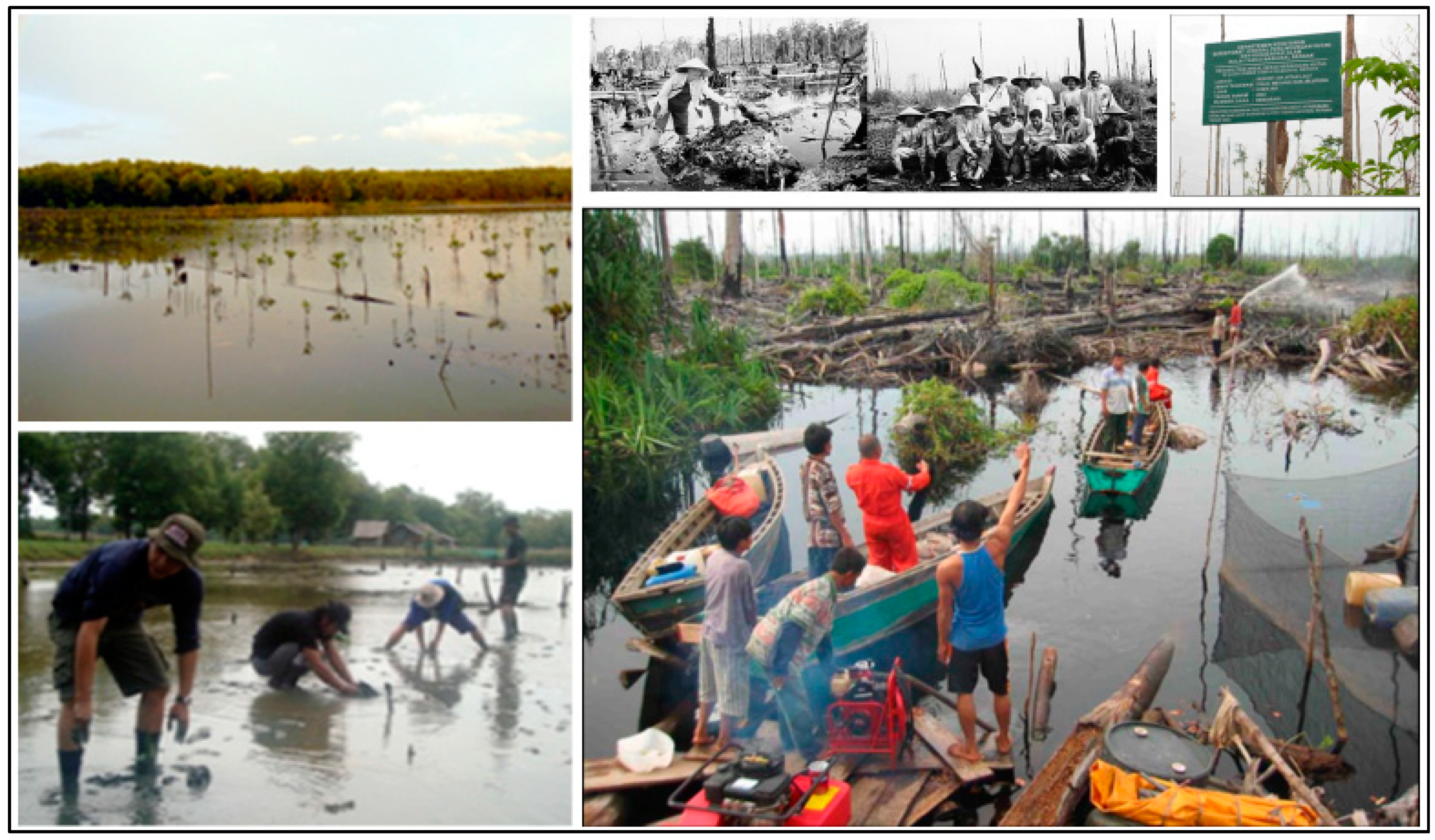
As an area affected by forest fire in 1997, various efforts have been made to rehabilitate mangrove forests in Sembilang Nasional Park (Figure 3) by involving Government and various stakeholders. Several related activities have been carried out [17]; (1) Integrated Swamp Development Project (ISDP) between Japan International Cooperation Agency (JICA) and Forest Fire Prevention Management Project/FFPMP in Northern Sembilang Nasional Park in 1997 to 2001; this project produce a document of descriptions, programs and suggestions to help planning, conservation, and control of resource use in buffer zones, (2) Forest Fire Prevention Management Project (FFPMP) by JICA in Sei Rambut Village in Northern Sembilang Nasional Park in 1997 to 2000, (3) Global Environment Facility (GEF) Project Berbak-Sembilang in 2000 to 2004; the purpose of this project are spatial planning, assessment, monitoring, and capacity building and environmental awareness; and (4) Climate Change, Forest and Peatlands in Indonesia project (CCFPI) in 2002 to 2005; this project consists of community based activities and policy development activities related to the protection and rehabilitation of swamp forests and peatlands in Indonesia.

2.2. Methodology

The methodology in this study is divided into five steps (Figure 4) including (1) a suit of data Landsat 5, Landsat 7 ETM+, and Landsat 8 OLI multi-temporal include preprocessing, (2) image classification using support vector machine (3) measurements accuracy, (4) Mangrove change using the Markov Chain and Cellular Automata model, and (5) validation. The description of each step of the research is as follows:

2.3. Data and Preprocessing

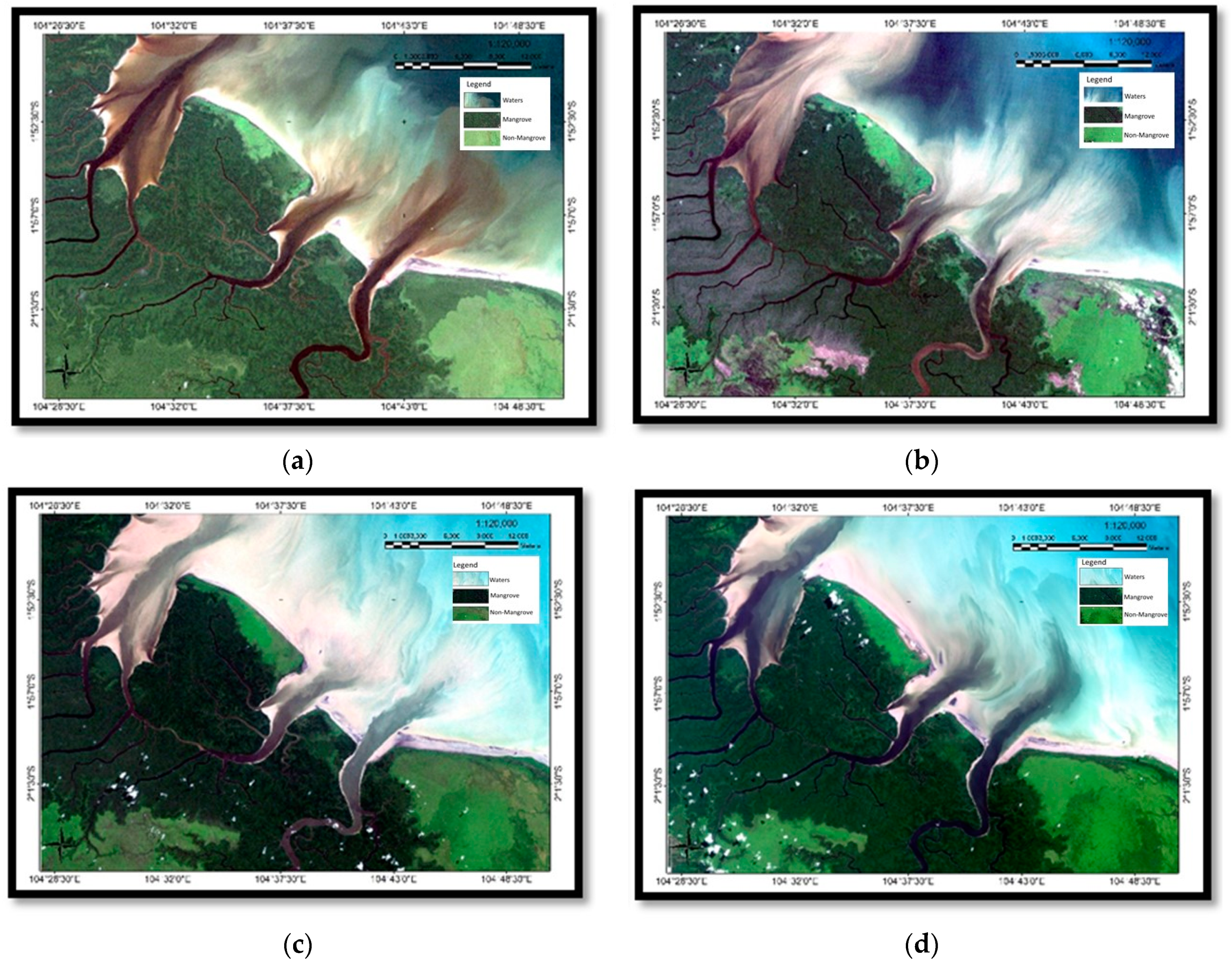
Landsat 5, Landsat 7 ETM+, and Landsat 8 OLI images acquired for 1989, 1998, 2002, and 2015 of 30 × 30 m2 spatial resolution derived from USGS. Landsat 2015 was used both to predict land cover in 2028. We also used the administrative boundary data of 1:50,000. The images were registered to the geographic coordinate projection using World Geodetic System 1984 (WGS-84). And auxiliary data of administrative boundaries data was obtained from Geospatial Information Agency (BIG). The data collected can be seen in Figure 5. The information of collected data can be seen in Table 1.

2.4. Classification

The support vector machine was used for classification of mangrove forests in study area. This classification was applied to the Landsat 5 images in 1989, Landsat 5 in 1998, Landsat 7 ETM+ in 2002, and Landsat 8 OLI images in 2015. This study was used support vector machine to fit an optimal separating hyperplane or set in a high or infinite-dimensional space to locate the optimal boundaries between classes. In this case the 3 classes defined previously there are mangroves, non-mangroves and water (Table 2).
Based on statistical theory, support vector machines operate by classifying two or more classes by studying for the best hyperplane that utilizes data at the separation point (super vector) even for a limited number of samples [74,75]. The support vector machine equation can be seen in the following Equation (1):
S V M ( F , λ ) ( R ) = s i g n   ( i N y i α i ( f R . f i ) + b )
where the SVM trainer of R is the class of region based on specific feature type F and specific scale λ. y i is the support vector class and αi (i = 1, ... , N) is decision coefficient with N is total of region. The support vectors are the f R is the feature vector the region and f i such that αi > 0, and b is a parameter found during the training.

2.5. Training Data Collection Scheme

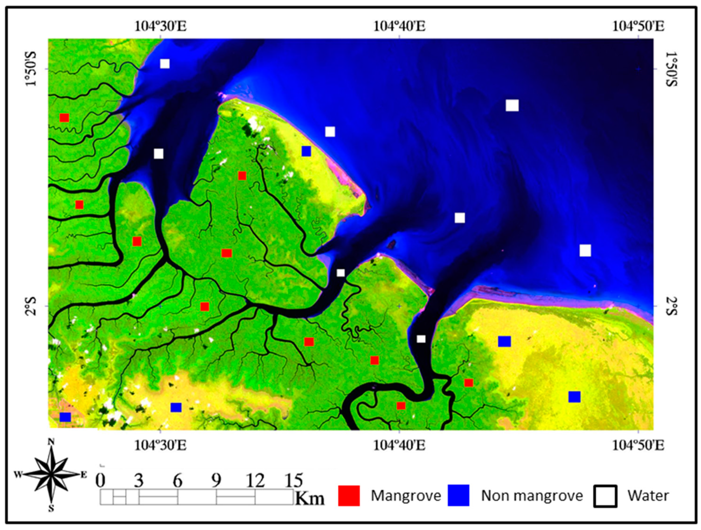
The training data were based on two different acquisition methods and incorporate field survey image interpretation using satellite data. Considering the time and access to the area is not always possible, GPS measurements were also impossible. The majority classes in Sembilang National Park where is not built-up area, the land cover only mangrove, non-mangrove (such as brush area), and water area. The distribution of training data can be seen in Figure 6. This study, mapping mangrove forest using Landsat 5, Landsat 7 ETM+, and Landsat 8 OLI images which spatial resolution is 30 m therefore training data of mangrove, non-mangrove and water patched on the field is more than 0.009 ha.

2.6. Accuracy Assessment

Classification accuracy was assessed based on the classification accuracy statistics, the error matrix (user/producer’s accuracy and omission/commission error), overall accuracy and kappa statistic [76]. Validation of the classification maps produced from the support vector machine implementation was performed against the set of validation pixels for each class collected following the procedure [77]. In addition to the classification statistics, the land cover classification was generated from the support vector machine algorithm and shows correspondence between the classification result and a reference data. The value of reference data was collected in 1458 pixels from the field in Equations (2)–(5).
Kappa   =   N   i = 1 r X i i   i = 1 r X i + ( X + i )   N 2   i = 1 r X i + ( X + i )   ×   100 %
Overall   Accuracy   =     i = 1 r X i i N   ×   100 %
User s   Accuracy   =   X i i X + i   ×   100 %
Producer s   Accuracy   =   X i i X + i   ×   100 %
where N is the number of all pixels used for observation, r is the number of rows in the error matrix (number of classes), Xii is diagonal values of the contingency matrix of row i and column i, X + i is column pixel number i, and Xi + row pixel number i.

2.7. Markov Chain

Modeling using Markov-Cellular Automata has been widely applied in several fields by researchers, including for the study of regional-scale land-use change, watershed management [78,79], regional monitoring cities [80,81,82,83], monitoring of plantation and agricultural areas [84], monitoring of erosion [85], simulating forest cover change [86], evaluating the integration of land use and climate change [87], and monitoring sand areas [88]. In 2015, Halmy et al. (2015) [88] used the Markov-Cellular Automata model to predict sand areas using Landsat TM 5 data, which yields 90% accuracy. The results show that the Markov-Cellular Automata model is a useful model for applying and predicting land cover.
Markov Chain determines how much land cover would be estimated to change from the latest date to the predicted date [89]. In this study, the Cellular Automata (CA) -Markov model was applied to predict the 2028 LULC in the Sembilang National Park area to identify variations in future mangrove land use. First, classified images from the period of 1989 and 1998; between 1998 to 2002, and 2002 until 2015 were selected as input into the model, to calculate matrix of conversion areas and conversion probabilities. The transition probability maps were used to produce maps of land use for the year of 2028. In an iterative process CA-Markov uses the transition probability maps of each land cover to establish the inherent suitability of each pixel to change from one land use type to another. The transition area matrix shows the total area (in cells) expected to change in the next period of 1989–1998, 1998–2002, and 2002–2015.
The prediction of land use changes is calculated by the following Equation (6) [89,90]:
S ( t ,   t + 1 ) = P i j   ×   S ( t )
where S (t) is the system status at time of t, S (t + 1) is the system status at time of t + 1; Pij is the transition probability matrix in a state [90]. If P is transition probability, namely the probability of converting current state to another state in next period [91], the expression is as follows:
P i j   =   [ P 11 P 12   P 1 n P 21 P 22   P 2 n P n 1 P n 2 P n n ]
( 0   P i j   1 )
where P is the transition probability; P i j stands for the probability of converting from current state i to another state j in next time; P n is the state probability of any time. Low transition will have a probability near 0 and high transition have probabilities near 1 [44].

2.8. Cellular Automata (CA)

The Cellular Automata (CA) is produces to determine iteration times, combining transition area matrix and potential transition maps as the CA local transition rule, land use map in the future could be simulated. In this study, Markov Chain results from data in the form of a transition probability matrix, transition area matrix, and a set of conditional probability images (1989–1998, 1998–2002) and actual land use maps in 2002 and 2015 were applied with the Cellular Automata model to obtain predictions of land cover in 2002 and 2015.
The CA model can be expressed as follows in Equation (9) [90]:
S ( t ,   t + 1 ) = f   ( S ( t ) ,   N )
where S is the set of limited and discrete cellular states, N is the Cellular field, t and t + 1 indicate the different times, and f is the transformation rule of cellular states in local space.

2.9. Validation

In terms of validating the CA-Markov predictions and evaluating the applied models results, validating process map predictions based on actual maps can be achieved. In this study for validating the model, the condition of land cover in 2002 and 2015 was estimated and compared with actual land use maps [56,92]. The precision of simulation or classification image results, pixel-by-pixel, is accessed via the kappa accuracy index.
Kappa index of agreement provided Kno, Klocation, KlocationStrata and Kstandard index. This statistic ranges from −1 (significantly worse than random) to 1 (perfect), but it typically lies between 0 and 1. Kno (kappa for no ability) showed the proportion between the actual map and the prediction map accurately determine the location, Klocation (kappa for location) showed the proportion between the actual map and the prediction map based on input at a location, Klocationstrata showed the proportion between the actual map and prediction map based on the number, and Kstandard (kappa index) aims to compare the proportion that is observed to be correct with the proportion that is expected due to probability [93]. The formulas for the summary statistics following Equations (10)–(13) [93,94]:
Κ n o =   ( M   ( m ) N   ( n ) ) ( P   ( p ) N   ( n ) )
Κ l o c a t i o n =   ( M   ( m )   N   ( m ) ) ( P   ( m ) N   ( m ) )
Κ l o c a t i o n s t r a t a =   ( M   ( m )   H ( m ) ) ( K   ( m ) H   ( m ) )
Κ s t a n d a r d =   ( M   ( m ) N   ( n ) ) ( P   ( p ) N   ( n ) )
where no information is defined by N(n), medium stratum level information by H(m), medium grid cell level information by M(m), perfect grid cell-level information given imperfect stratum-level information by K(m) mean, and perfect grid cell-level information across the landscape by P(p).

3. Results

3.1. Land Cover Classification in 1989, 1998, 2002, and 2015

The land cover classification was obtained from Landsat 5, Landsat 7 ETM+, and Landsat 8 OLI Images in 1989, 1998, 2002, and 2015 using the support vector machine algorithm in Sembilang National Park. Land cover classes were categorized into three: Mangroves, Non-mangroves, and Water.
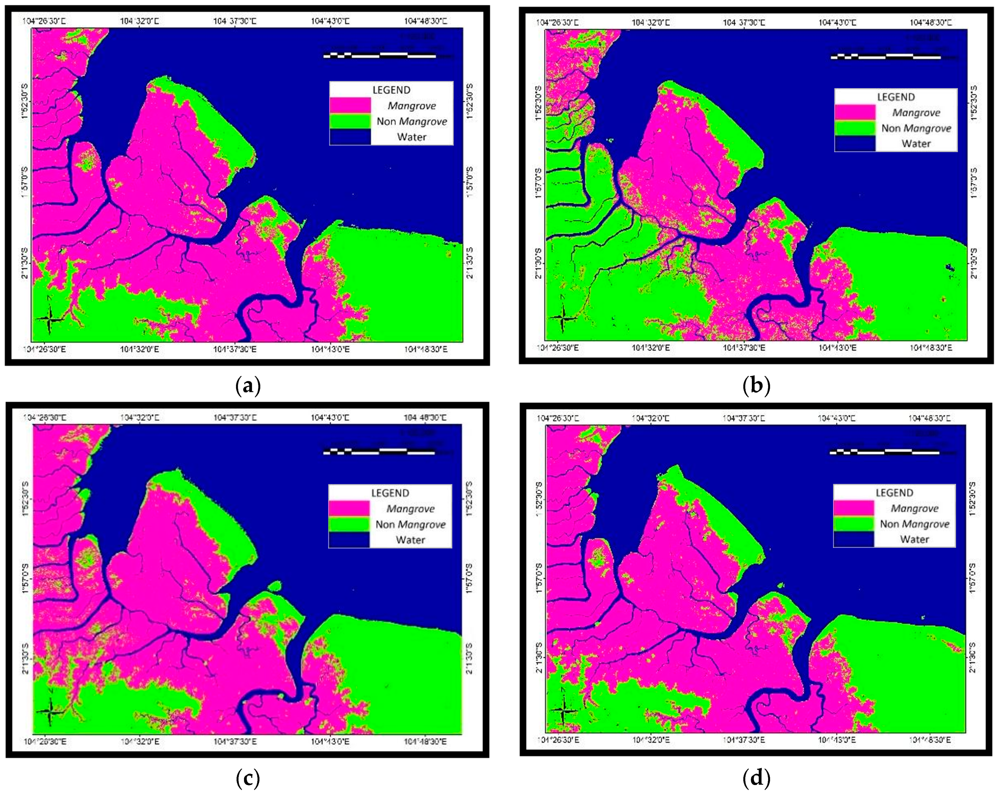
We obtained the land cover map from the classification algorithm by use of the support vector machine (Figure 7). We identified three dominant classes in the study area including Mangrove, Non-mangrove, and Water. Based on Figure 7b, for the years 1989 to 1998 we can see visually, there was the decrease of Mangrove forest because of forest fire, while, from the years 1998 to 2015 there was the significant increase of Mangrove forest. The accuracy assessment of classification obtained by each year can be seen on Table 3, Table 4, Table 5 and Table 6.
The confusion matrix shows accuracy assessment of classifications for the years 1989, 1998, 2002, and 2015 (Table 3, Table 4, Table 5 and Table 6). The classification provided from the use of training data indicated that land cover reliability mapped, showed that all categories had above 90% rate of overall accuracy and kappa statistic. The discrimination of mangrove class also shows good accuracy with a commission error in years 1989, 1998, 2002, and 2015 of 0.4%, 2.8%, 3.2%, and 1.3%, respectively. In addition, the commission error in 1989, 1998, 2002, and 2015 of 0%, 0.9%, 1.3%, and 0%, respectively.

3.2. Land Cover Change Classification

The support vector machine classification produces an area of land-use classes (Mangrove, Non-mangrove, and Water). Overall, each land-use class area for years 1989, 1998, 2002, and 2015 can be seen in Table 7.
The area occupied by each class in 1989 was: Mangrove 58,145.5 ha (26.2%), Non-mangrove 53,265.4 ha (24.1%), and 109,886 ha (49.6%). In 1998, Mangrove area was decreased to 36,847.4 ha (16.6%), Non-mangrove area was increased to 73,327.4 ha (33.1%) and the Water area was increased to 111,112 ha (50.2%). In contrast to 1989, mangrove areas show increased trends both in 2002 and 2015. In 2002, that the Mangrove area was increased to 55,548.3 ha (25.1%), Non-mangrove has decreased to 58,419.1 ha (26.3%), and the water area has decreased to 107,329 ha (48.5%). In 2015, the Mangrove areas has increased to 60,697.5 ha (27.4%), Non-mangrove areas has decrease to 51,965.8 ha (23.4%), and the Waters area has increased to 108,633 ha (49.1%).

3.3. Transition Matrix and Transition Probability Matrix for the Land Cover

The transition matrix area and transition probability matrix for years 1989–1998, 1998–2002, and 2002–2015 can be seen in Table 8 and Table 9. The transition probability matrix from 1989 to 2015 then used to predict mangrove forest change in the year 2028. Validation of Markov-Cellular Automata identify map was carried out by comparing prediction Mangrove forest map of the year 2028 with the support vector machine 2015 classified Mangrove forest map.
The transition probability matrix for years 1989–1998, 1998–2002, and 2002–2015 show that changing mangroves to non-mangroves from 1989 to 1998 is 0.3 and probability decreased by 0.2 in 1998–2002 (Table 8). When transition of non-mangrove into mangrove was observed, the transition probability was very low in 1989–1998 of 0.1. The probability of changing non-mangroves to mangrove areas in 2002–2015 decreased by 0.2. Mangrove, non-mangrove, and waters classes for the period 1989–1998, 1998–2002, and 2002–2015 have a probability value above 0 can change to the other classes, indicating the possibilities appropriate for analyzing changes in existing land cover.
Land-cover change was shown as transition matrix area in 1989–1998, 1998–2002 and 2002–2015 (Table 9). The probability transition shows that from 1989 to 1998, mangroves had the highest chance of becoming non-mangroves with a prediction of pixel allocations of 142,756 pixels or equivalent with 12,848.4 ha (area pixels = 900 m2). In addition, in the same period, waters had the most significant chance of becoming mangrove with the prediction of pixel allocations of 141,087 equivalent with 12,697.8 ha. The 1998–2002 period shows that mangroves, non-mangroves, and water have the highest chance of becoming changed with several pixel allocations.

3.4. Prediction of Land Cover Change in Year 2002 and 2015

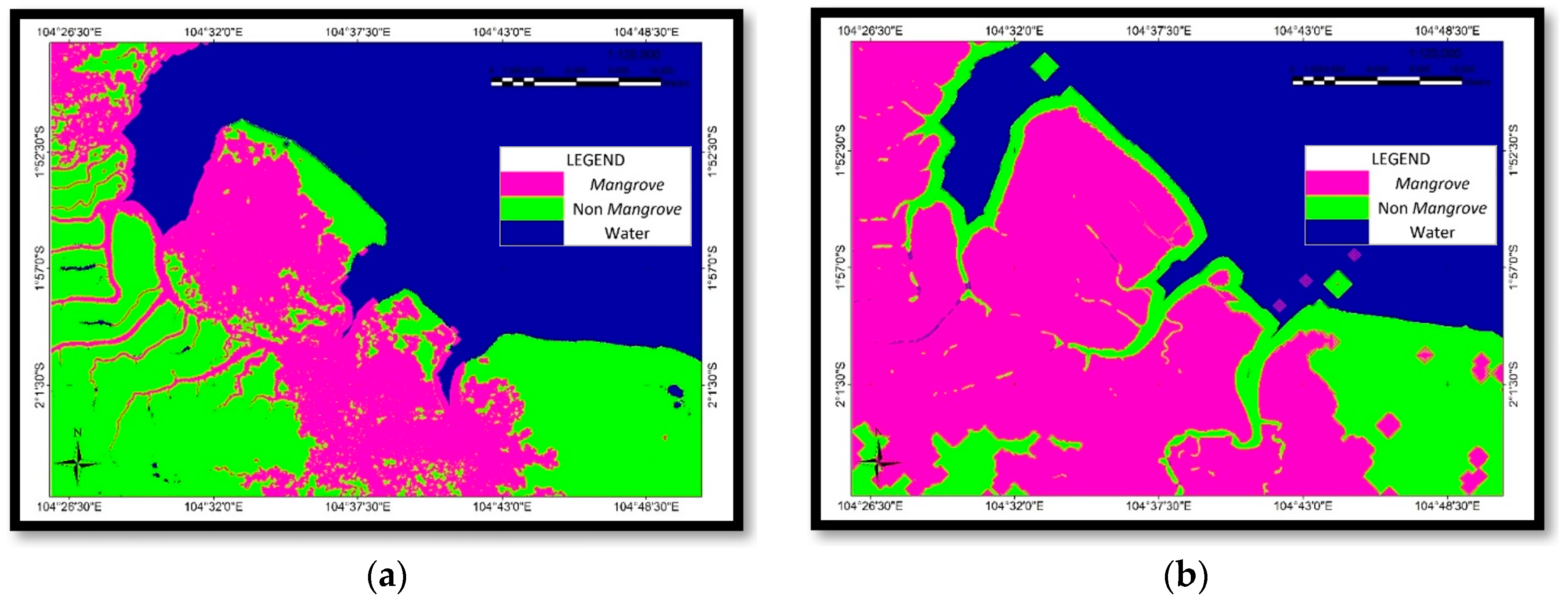
The simulation results of the Markov-CA model to predict land cover in 2002 and 2015 were shown in Figure 8, while the area of land cover prediction map in 2002 and 2015 can be seen in Table 10.
The area occupied by each class in 2002 (prediction) was: Mangrove of 42,224.1 ha (19.1%), Non-mangrove of 77,012.6 ha (34%), and Water of 10,059.9 ha (46.1%) (Table 10). In contrast, 2015 (prediction), Mangrove area was increased to 86,245.2 ha (38.9%), while both Non-mangrove area and Water were decreased to 47,087.1 ha (21.2%) and 87,964.2 ha (39.7%), respectively.

3.5. Kappa Index Agreement

Kappa evaluate how well classification or modeling performs excluding chance agreement [93]. In this study, kappa was used to assess the agreement between the 2002 and 2015 actual land cover maps and simulations. Kappa index agreement of prediction years 2002 and 2015 can be seen in Table 11. We found that the lowest kappa index agreement of 2002 (prediction) is 0.7 as Kstandard, while the highest kappa index agreement of 2002 is 0.8 as Klocation and KlocationStrata. In addition, the lowest kappa index agreement of 2015 (prediction) is 0.7 as Kstandard, while the highest kappa index agreement of 2015 (prediction) is 0.8 as Klocation and KlocationStrata. According to Gwet (2014) [95], Kno and Kstandard obtained from both prediction map in 2002 and 2015 indicated substantial agreement, while Klocation and KlocationStrata obtained from both prediction map in 2002 and 2015 indicated almost perfect agreement.

3.6. Prediction of Land Cover Change in 2028

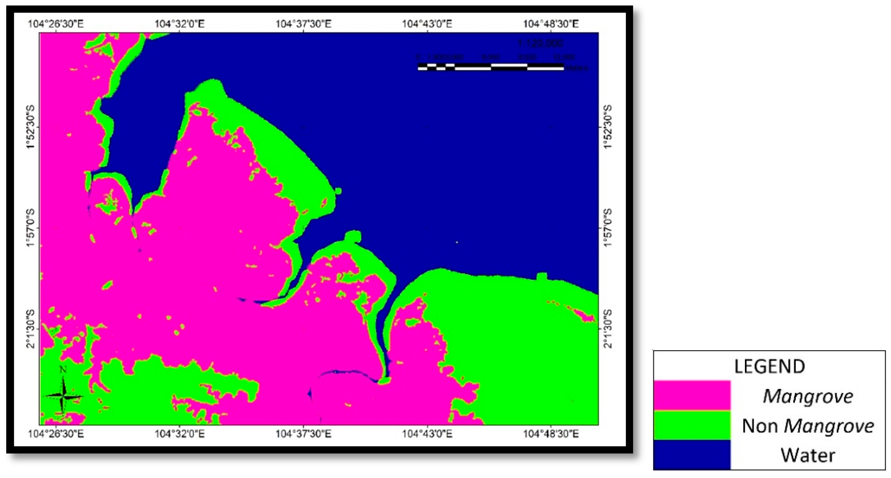
Land cover change years 2028 prediction using land over obtained from land cover year 2015. The 2015 land cover data were used for the base map, the potential transition map, and a transition area matrix for 2002–2015. The future land cover models are predicted, as shown in Figure 9 while the prediction area for 2028 is seen in Table 12.
Table 12 shows the period between 2015 and 2028, area of Mangroves increased from 27.4% to 31% or 7974.8 ha, while the area of Non-mangrove also increased from 23.4% to 25.1% or 3725.3 ha, and Water area decreased from 49.1% to 43.8% or 11,696.7 ha. In general, the area of classification results in 1989, 1998, 2002, and 2015 and the predicted results for 2028 can be seen in Table 12.

4. Discussion

4.1. Imagery Data on This Study

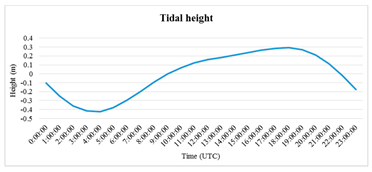
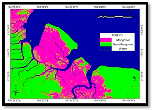
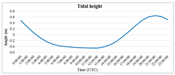
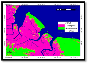
Landsat data was used in this study because it maps general land cover classes at a spatial resolution of 30 m for large areas. The identification of mangrove cover based on satellite images is not free from ambiguity. The problems usually occur related to the class representation, mixed pixel effects, and tidal effects [96]. For selecting the images, different seasons and atmospheric conditions must be considered [97]. According to Darmawan et al. (2015) mangrove identification and estimation of above-ground mangrove forest biomass are influenced by tidal height [98]. Therefore, the acquisition of Landsat 5 was carried out on 17 May 1989, at 02:39:43 UTC, Landsat 5 on 24 April 1998, at 02:48:21, Landsat 7 ETM+ on 30 June 2002, at 02:59:41, and Landsat 8 OLI on 26 June 2015, at 03:10:34 occurs at the same tides which are affected by the tidal height (Table 13), and also in April–June in South Sumatra has entered the dry season. In Indonesia, there are only two seasons, namely the rainy season and the dry season. It means that for each tidal effect, the Landsat image and atmospheric conditions are at the same conditions.

4.2. Accuracy Assessment

The sufficient number of training data and the selection of classification approaches are essential factors in successful classification [99,100]. In this study, training data were collected from more acceptable spatial resolution imagery. We collected a total of 1042 training pixels covering the Sembilang National Park of the area mapped. In this study, the amount both of the training and testing used are unbalance data. There are 432 training pixels with the primary class of mangrove, 333 training pixels labeled as land, and 277 training pixels labeled as water. The number of training data was following [101]. The training data size should not be smaller than 10 to 30 times the number of bands for each object. All pixels were selected randomly following to uniform in ground truth data. According to some researchers, balancing samples in classification is a controversial topic [102,103,104].
In some cases, unbalanced data was inevitable due to the complexity and heterogeneous landscapes in the study area when choosing training data [105]. Therefore, this problem can be handled using the appropriate classifications approach, such as a vector machine. The support vector machine for handling unbalanced data in the classification process is the best choice, proven in high accuracy (Table 14).
The classification accuracy obtained from Landsat 1989, 1998, 2002, and 2015 indicated that the support vector machine was the right option for mangrove mapping based on an unbalance training sample. In this study, the overall accuracy of the land cover maps for 1989 (99.8%), 1998 (98.5%), 2002 (97.9%), and 2015 (99.5%) were achieved. All accuracy indicators of overall accuracy, kappa statistics, Mangrove user accuracy, and Mangrove producer accuracy were above 90%. Table 14 shows that the support vector machine classifier’s performance can dramatically decrease with a relatively small number of mislabeled examples [76]. According to Mountrakis (2011) [76], support vector machines are not relatively sensitive to training sample size, and some literature has improved support vector machines to work successfully with limited quantity and quality of training data [76].

4.3. Matrix Probability Transition

The probability matrix is a factor that sets the trend of change in surrounding cells as a function of cell conditions themselves. The CA-Markov was applied for simulation of mangrove cover changed. Three intervals period were used in this study, including an interval of 9 years (1989–1998), an interval of 4 years (1998–2002), and 13 years (2002–2015). Each interval represents each land cover category projections, while the third interval is determined by the results of project accuracy in 2028.
The probability transition matrix had been done for the interval in 9 years (1989–1998), an interval of 4 years (1998–2002), and 13 years (2002–2015) (Figure 10). Figure 10, the interval of 9 years (1989–1998), indicated that more than half of the Mangrove was changed into Non-mangrove areas (34.8%). This result was related to the Forestry Research and Development Agency (2013) that South Sumatra experienced relatively high deforestation during the 1990, resulting in a decrease in mangrove forest cover due to forest fires in 1997–1998. The worst of them occurred in 1997 during the dry weather fostered by El Niño [29]. At the same time, there was no change in Mangrove becoming Water. In the same interval years, 82% of Non-mangrove remained unconverted. So, the water 84.8% remained unconverted. The four-year (1998–2002) interval showed a positive change concerning the Mangrove forest recovery, which is showed 66.4% Non-mangrove and 8.3% Water shifted to mangrove areas. The increasing Mangrove areas resulted in better management by the government in Sembilang National Park. It is also proven from 13 years (2002–2015), indicating that 81.1% of Mangroves remain unconverted. Totally 22.3% Non-mangrove and 7.2% Water changed to Mangrove areas. The increase of Mangrove areas indicated better management in Sembilang National Park.

4.4. Land Cover Area in Years 1989, 1998, 2002, 2015 and Predicted 2028

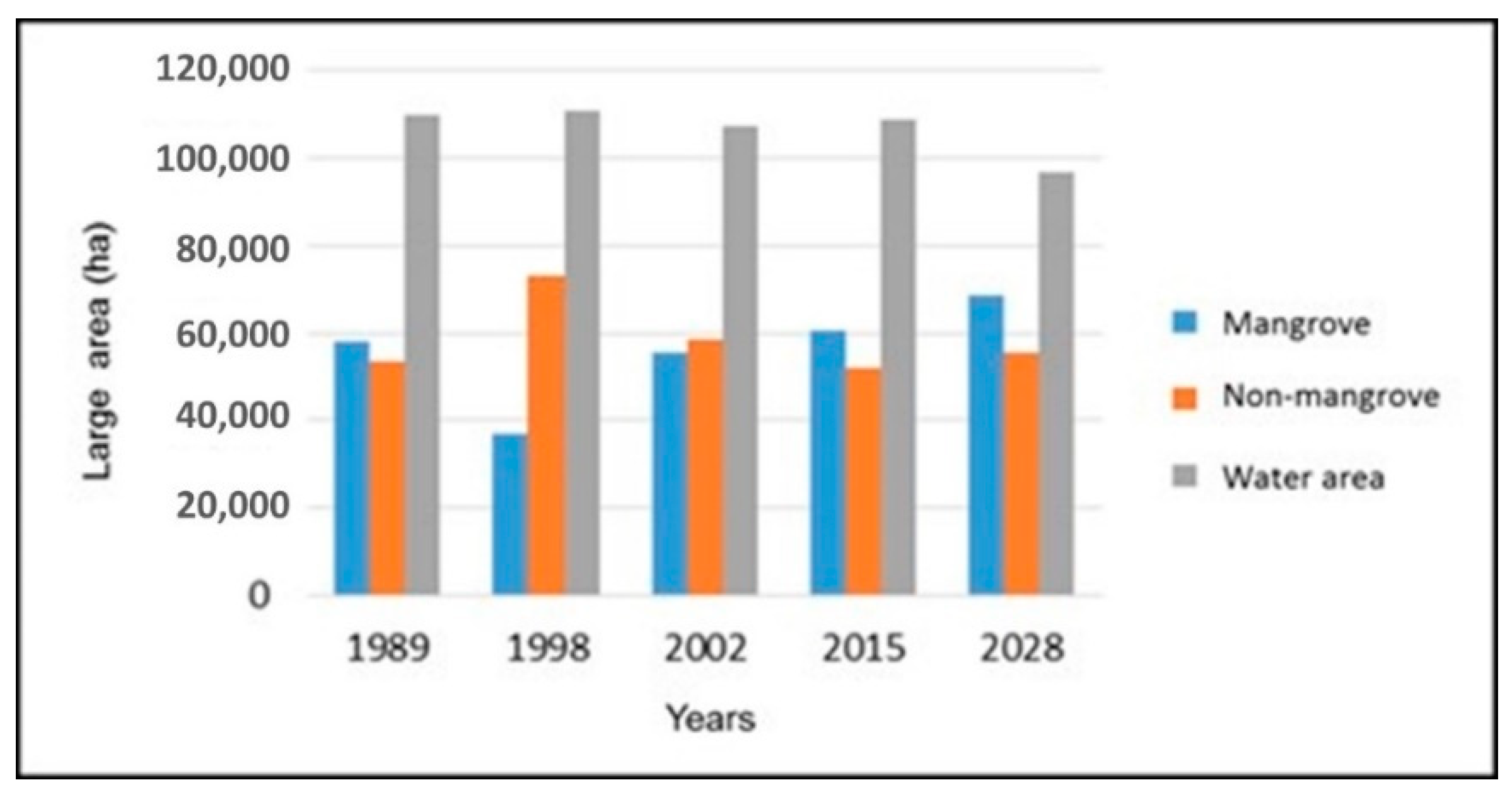
The statistics area (ha) trend was derived from the support vector machine classification for 1989, 1998, 2002, 2015, and prediction 2028 (Figure 11). In 1989–2018, the trend of mangrove land cover fluctuated indicated the lowest mangrove area is in 1998 of 36,847.4 ha, and the highest mangrove area predicted in 2028 of 68,672.3 ha. In the interval years of 1989–1998, the loss mangroves in Sembilang National Park are 21,298.1 ha. The decrease of mangrove was caused by the worst forest fires in Indonesia in 1997 [29]. However, in 1998–2028, the increase of mangrove forest became 55,548.3 ha in 2002, 60,697.5 ha in 2015, and 68,672.3 ha in 2028. The highest rate of increasing mangrove forests was in 1998–2002 of 8.4%. The increase of the mangrove forest area indicated that the government had succeeded in mangrove rehabilitation management.

5. Conclusions

In this study, we calculated mangrove forest changes areas in Sembilang National Park, Banyuasin, Indonesia from 1989, 1998, 2002, 2015, and predicted mangrove forest areas in 2028 using the support vector machine algorithm and the Markov-Cellular Automata model. Based on the historical land cover from 1989 to 2015, the study has attempted to detect, simulate and predict the future expansion trends up to 2028, with a specific empirical focus on changes in the mangrove forest area. The results showed that the mangrove forest area from 1989 to 1998 has decreased around 9.6%. The worst forest fires caused the decrease of mangrove forests in Indonesia in 1997. However, the Indonesian government keeps trying to rehabilitate mangrove forests in Sembilang National Park as the largest mangrove forest. It was proven that the mangrove area has increased by 8.4% between 1998 and 2002, and 2.3% in 2002–2015. Other results showed that the mangroves area has continued to increase from 2015 to 2028 by 27.4% to 31% (7974.8 ha). The increase of the mangrove forest area indicated that the government had succeeded in mangrove rehabilitation management.

Author Contributions

Conceptualization, S.D., D.K.S. and K.W.; Data curation, M.K.S.; Formal analysis, S.D. and R.H.; Methodology, S.D., D.K.S., K.W. and R.H.; Validation, M.K.S.; Visualization, A.T. and M.K.S.; Writing—original draft, S.D. and A.T.; Writing—review & editing, R.H. All authors have read and agreed to the published version of the manuscript.

Funding

This research was funded by Ministry of Research and Technology/National Agency for Research and Innovation (Kemenristek/BRIN), Number: 378/B.05/LPPM-Itenas/IV/2020.

Acknowledgments

In addition, the researcher would like to acknowledge the funding support from Ministry of Research and Technology/National Agency for Research and Innovation (Kemenristek/BRIN) and LPPM Itenas Bandung.

Conflicts of Interest

The authors declare no conflict of interest.

References

  1. Nybakken, J.W.; Eidman, H.M. Biologi Laut: Suatu Pendekatan Ekologis; PT Gramedia Pustaka Utama: Jakarta, Indonesia, 1992; ISBN 979403018X 9789794030189. [Google Scholar]
  2. Romimohtarto, K. Biologi Laut: Ilmu Pengetahuan Tentang Biota Laut/Kasijan Romimohtarto, Sri Juwana; Djambatan: Jakarta, Indonesia, 2001; ISBN 9794284009. [Google Scholar]
  3. Donato, D.C.; Kauffman, J.B.; Murdiyarso, D.; Kurnianto, S.; Stidham, M.; Kanninen, M. Mangroves among the most carbon-rich forests in the tropics. Nat. Geosci. 2011, 4, 293–297. [Google Scholar] [CrossRef]
  4. Paillon, C.; Wantiez, L.; Kulbicki, M.; Labonne, M.; Vigliola, L. Extent of Mangrove Nursery Habitats Determines the Geographic Distribution of a Coral Reef Fish in a South-Pacific Archipelago. PLoS ONE 2014, 9, e105158. [Google Scholar] [CrossRef] [PubMed]
  5. Barbier, E.B.; Hacker, S.D.; Kennedy, C.; Koch, E.W.; Stier, A.C.; Silliman, B.R. The value of estuarine and coastal ecosystem services. Ecol. Monogr. 2011, 81, 169–193. [Google Scholar] [CrossRef]
  6. Brown, D. Mangrove: Nature’s Defences Against Tsunamis; Environmental Justice Foundation: London, UK, 2004. [Google Scholar]
  7. Walters, B.B.; Rönnbäck, P.; Kovacs, J.M.; Crona, B.; Hussain, S.A.; Badola, R.; Primavera, J.H.; Barbier, E.; Dahdouh-Guebas, F. Ethnobiology, socio-economics and management of mangrove forests: A review. Aquat. Bot. 2008, 89, 220–236. [Google Scholar] [CrossRef] [Green Version]
  8. Giesen, W. Indonesia’s Mangrove: An Update on Remaining Area and Main Management Issues; Asian Wetland Bureau (AWB): Wageningen, The Netherlands, 1993. [Google Scholar]
  9. Spalding, M.; Blasco, F.; Field, C. World Mangrove Atlas; FAO: Rome, Italy, 1997; p. 178. [Google Scholar]
  10. Suwignyo, R.A.; Ulqodry, T.Z.; Halimi, E.S.; Dwipa, H.S. Hutan Mangrove Pada Masyarakat. In Proceedings of the Lokakarya Pembentukan Kelompok Kerja Mangrove Daerah (KKMD) Provinsi Sumatera Selatan Balai Pengelolaan Hutan Mangrove Wilayah II Direktorat Jenderal Bina Pengelolaan Daerah Alir, Palembang, Indonesia, 26 May 2011. [Google Scholar]
  11. Ekosistem Sembilang—Taman Nasional Berbak; TFCA Sumatera: Jakarta, Indonesia. Available online: http://tfcasumatera.org/bentang_alam/ekosistem-sembilang-taman-nasional-berbak/ (accessed on 4 October 2020).
  12. Lubis, I.R.; Suryadiputra, I.N.N. Upaya pengelolaan terpadu hutan rawa gambut bekas terbakar diwilayah Berbak-Sembilang. In Kebakaran di lahan rawa/gambut di Sumatera: Masalah dan Solusi. Prosiding Semiloka; CIFOR: Bogor, Indonesia, 2004; pp. 105–119. [Google Scholar]
  13. Tirtakusumah, R. Pengelolaan Hutan Mangrove Jawa Barat dan Beberapa Pemikiran untuk Tindak Lanjut. In Proceedings of the Dalam Prosiding Seminar V Ekosistem Mangrove, Jember, Indonesia, 3–6 August 1994; pp. 3–6. [Google Scholar]
  14. Dahuri, R.; Rais, J.; Ginting, S.P.; Sitepu, M.J. Integrated Coastal and Marine Resource Management, 2nd ed.; PT. Pradnya Paramita: Jakarta, Indonesia, 2001; p. 328. [Google Scholar]
  15. Anderson, I.P.; Bowen, R. Fire Zones and the Threat to the Wetlands of Sumatra, Indonesia; Report; European Union Ministry of Forestry: Palembang, Indonesia, 2000; pp. 1–46. [Google Scholar]
  16. Barber, C.V.; Schweithelm, J. Trial by Fire: Forest Fires and Forestry Policy in Indonesia’s Era of Crisis and Reform; Report; In collaboration with WWF-Indonesia and Telapak Indonesia Foundation; World Resources Institute (WRI), Forest Frontiers Initiative: South Jakarta, Indonesia, 2000; ISBN 1569734089. [Google Scholar]
  17. Lubis, I.R.; Suryadiputra, I.N.N. Upaya Pengelolaan Terpadu Hutan Rawa Gambut Bekas Terbakar di WIlayah Berbak-Sembilang; CIFOR: Bogor, Indonesia, 2003; ISBN 9793361492. [Google Scholar]
  18. Parameswaran, K.; Nair, S.K.; Rajeev, K. Impact of Indonesian forest fires during the 1997 El Nino on the aerosol distribution over the Indian Ocean. Adv. Space Res. 2004, 33, 1098–1103. [Google Scholar] [CrossRef]
  19. Page, S.E.; Siegert, F.; Rieley, J.O.; Boehm, H.-D.V.; Jaya, A.; Limin, S. The amount of carbon released from peat and forest fires in Indonesia during 1997. Nature 2002, 420, 61–65. [Google Scholar] [CrossRef]
  20. Harrison, M.E.; Page, S.E.; Limin, S.H. The global impact of Indonesian forest fires. Biologist 2009, 56, 156–163. [Google Scholar]
  21. Boer, C. Forest and fire suppression in East Kalimantan, Indonesia. In Proceedings of the International Conference on Community Involvement in FIRE Management; Food and Agriculture Organization of the United Nations (FAO), Regional Office for Asia and the Pacific: Rome, Italy, 2002; pp. 69–71. [Google Scholar]
  22. BAPPENAS (National Development Planning Agency); Asian Development Bank (ADB). Causes, extent, impact and costs of 1997/98 fires and drought. Final Report, Annex 1 and 2; ADB: Jakarta, Indonesia, 1999. [Google Scholar]
  23. Tacconi, L. Kebakaran Hutan di Indonesia: Penyebab, Biaya Dan Implikasi Kebijakan; CIFOR: Bogor, Indonesia, 2003. [Google Scholar]
  24. Glover, D.; Jessup, T. The Indonesian fires and haze of 1997: The economic toll. In Proceedings of the Economy and Environment Program for SE Asia (EEPSEA) Singapore and the World Wildlife Fund (WWF) Indonesia, Jakarta, Indonesia, May 1998. [Google Scholar]
  25. Anderson, I.P.; Bowen, M.R.; Imanda, I.D. Muhnandar Forest Fire Prevention and Control Project Forest Fire Prevention and Control Project Vegetation Fires in Indonesia: The Fire History of the Sumatra Provinces 1996–1998 As a Predictor of Future Areas At Risk; Report; Balai Inventaris dan Perpetaan Hutan Wilayah II and Kanwil Kehutanan dan Perkebunan: Palembang, Indonesia, 1999. [Google Scholar]
  26. CIFOR. A Review of Fire Projects in Indonesia (1982–1998); CIFOR: Bogor, Indonesia, 1999; ISBN 9798764307. [Google Scholar]
  27. Legg, C.A.; Laumonier, Y. Fires in Indonesia, 1997: A remote sensing perspective. Ambio 1999, 28, 479–485. [Google Scholar] [CrossRef]
  28. Bowen, M.R.; Bompard, J.M.; Anderson, I.P.; Guizol, P.; Gouyon, A. Anthropogenic Fires in Indonesia: A View from Sumatra; CIFOR: Bogor, Indonesia, 2001; pp. 41–66. [Google Scholar]
  29. Podgorny, I.A.; Li, F.; Ramanathan, V. Large aerosol radiative forcing due to the 1997 Indonesian forest fire. Geophys. Res. Lett. 2003, 30. [Google Scholar] [CrossRef]
  30. Pemerintah Republik Indonesia. Undang-Undang Nomor 5 Tahun 1990 Tentang Konservasi Sumber Daya Alam Hayati dan Ekosistemnya; Pemerintah Republik Indonesia: Jakarta, Indonesia, 1990; Volume 1988, pp. 1–26. [Google Scholar]
  31. Verburg, P.H.; Schot, P.P.; Dijst, M.J.; Veldkamp, A. Land use change modelling: Current practice and research priorities. GeoJournal 2004, 61, 309–324. [Google Scholar] [CrossRef]
  32. Sohl, T.; Sleeter, B. Role of remote sensing for land-use and land-cover change modeling. In Remote Sensing of Land Use and Land Cover: Principles and Applications; Giri, C.P., Ed.; CRC Press: Boca Raton, FL, USA, 2012; pp. 225–239. [Google Scholar]
  33. Rogan, J.; Chen, D. Remote sensing technology for mapping and monitoring land-cover and land-use change. Prog. Plan. 2004, 61, 301–325. [Google Scholar] [CrossRef]
  34. Gómez, C.; White, J.C.; Wulder, M.A. Optical remotely sensed time series data for land cover classification: A review. ISPRS J. Photogramm. Remote Sens. 2016, 116, 55–72. [Google Scholar] [CrossRef] [Green Version]
  35. Singh, A. Review article digital change detection techniques using remotely-sensed data. Int. J. Remote Sens. 1989, 10, 989–1003. [Google Scholar] [CrossRef] [Green Version]
  36. Lu, D.; Mausel, P.; Brondizio, E.; Moran, E. Change detection techniques. Int. J. Remote Sens. 2004, 25, 2365–2401. [Google Scholar] [CrossRef]
  37. Alqurashi, A.; Kumar, L. Investigating the use of remote sensing and GIS techniques to detect land use and land cover change: A review. Adv. Remote Sens. 2013. [Google Scholar] [CrossRef] [Green Version]
  38. Bolstad, P.; Lillesand, T.M. Rapid maximum likelihood classification. Photogramm. Eng. Remote Sens. 1991, 57, 67–74. [Google Scholar]
  39. Franklin, J.; Woodcock, C.E.; Warbington, R. Multi-attribute vegetation maps of forest service lands in California supporting resource management decisions. Photogramm. Eng. Remote Sens. 2000, 66, 1209–1218. [Google Scholar]
  40. Dewan, A.M.; Yamaguchi, Y.; Rahman, M.Z. Dynamics of land use/cover changes and the analysis of landscape fragmentation in Dhaka Metropolitan, Bangladesh. GeoJournal 2012, 77, 315–330. [Google Scholar] [CrossRef]
  41. Guild, L.S.; Cohen, W.B.; Kauffman, J.B. Detection of deforestation and land conversion in Rondonia, Brazil using change detection techniques. Int. J. Remote Sens. 2004, 25, 731–750. [Google Scholar] [CrossRef]
  42. Yuan, D.; Elvidge, C. NALC land cover change detection pilot study: Washington DC area experiments. Remote Sens. Environ. 1998, 66, 166–178. [Google Scholar] [CrossRef]
  43. Lambin, E.F.; Baulies, X.; Bockstael, N.; Fischer, G.; Krug, T.; Leemans, R.; Moran, E.F.; Rindfuss, R.R.; Sato, Y.; Skole, D.; et al. Land-Use and Land-Cover Change (LUCC): Implementation Strategy; IGBP Report No. 48, IHDP Report No. 10; International Geosphere-Biosphere Programme (IGBP), International Human Dimension Programme on Global Environmental Change (IHDP): Stockholm, Sweden, 1999; p. 125. [Google Scholar]
  44. Behera, M.D.; Borate, S.N.; Panda, S.N.; Behera, P.R.; Roy, P.S. Modelling and analyzing the watershed dynamics using Cellular Automata (CA)-Markov model—A geo-information based approach. J. Earth Syst. Sci. 2012, 121, 1011–1024. [Google Scholar] [CrossRef] [Green Version]
  45. Zhang, Y.; Gong, H.; Zhao, W.; Li, X. Analyzing the mechanism of land use change in Beijing City from 1990 to 2000. Resour. Sci. 2007, 29, 206–213. [Google Scholar]
  46. Memarian, H.; Balasundram, S.K.; Talib, J.B.; Teh, C.; Sung, B.; Sood, A.M.; Abbaspour, K. Validation of CA-Markov for Simulation of Land Use and Cover Change in the Langat Basin, Malaysia. J. Geogr. Inf. Syst. 2012, 4, 542–554. [Google Scholar] [CrossRef] [Green Version]
  47. Huang, W.; Liu, H.; Luan, Q.; Jiang, Q.; Liu, J.; Liu, H. Detection and prediction of land use change in Beijing based on remote sensing and GIS. Int. Arch. Photogramm. Remote Sens. Spat. Inf. Sci. 2008, 37, 75–82. [Google Scholar]
  48. Weng, Q. Land use change analysis in the Zhujiang Delta of China using satellite remote sensing, GIS and stochastic modelling. J. Environ. Manag. 2002, 64, 273–284. [Google Scholar] [CrossRef] [PubMed] [Green Version]
  49. Benenson, I.; Torrens, P. Geosimulation: Automata-Based Modeling of Urban Phenomena; John Wiley & Sons Inc.: Hoboken, NJ, USA, 2004; ISBN 0470843497. [Google Scholar]
  50. Candau, J.; Rasmussen, S.; Clarke, K.C. A coupled cellular automaton model for land use/land cover dynamics. In Proceedings of the Fourth International Conference on Integrating GIS and Environmental Modeling (GIS/EM4): Problems, Prospects and Research Needs, Banff, AB, Canada, 2–8 September 2000. [Google Scholar]
  51. Koomen, E.; Rietveld, P.; Nijs, T. Modelling land-use change for spatial planning support. Ann. Reg. Sci. 2008, 42, 1–10. [Google Scholar] [CrossRef] [Green Version]
  52. Torrens, P.M.; Benenson, I. Geographic automata systems. Int. J. Geogr. Inf. Sci. 2005, 19, 385–412. [Google Scholar] [CrossRef] [Green Version]
  53. Houet, T.; Hubert-moy, L. Modelling and Projecting Land-Use and Land-Cover Changes with a Cellular Automaton in Considering Landscape Trajectories: An Improvement for Simulation of Plausible Future States. EASeL eProceedings 2006, 5, 63–76. [Google Scholar]
  54. Yirsaw, E.; Wu, W.; Shi, X.; Temesgen, H.; Bekele, B. Land Use/Land Cover change modeling and the prediction of subsequent changes in ecosystem service values in a coastal area of China, the Su-Xi-Chang region. Sustainability 2017, 9, 1204. [Google Scholar] [CrossRef] [Green Version]
  55. Fei, S.X.; Shan, C.H.; Hua, G.Z. Remote sensing of mangrove wetlands identification. Procedia Environ. Sci. 2011, 10, 2287–2293. [Google Scholar] [CrossRef] [Green Version]
  56. Chen, C.F.; Son, N.T.; Chang, N.B.; Chen, C.R.; Chang, L.Y.; Valdez, M.; Centeno, G.; Thompson, C.A.; Aceituno, J.L. Multi-decadal mangrove forest change detection and prediction in honduras, central america, with landsat imagery and a markov chain model. Remote Sens. 2013, 5, 6408–6426. [Google Scholar] [CrossRef] [Green Version]
  57. Aghighi, H.; Trinder, J.; Lim, S.; Tarabalka, Y. Improved adaptive Markov random field based super-resolution mapping for mangrove tree identification. ISPRS Ann. Photogramm. Remote Sens. Spat. Inf. Sci. 2014, 2, 61. [Google Scholar] [CrossRef] [Green Version]
  58. Dan, T.T.; Chen, C.F.; Chiang, S.H.; Ogawa, S. Mapping and change analysis in mangrove forest by using Landsat imagery. ISPRS Ann. Photogramm. Remote Sens. Spat. Inf. Sci. 2016, 3, 109. [Google Scholar] [CrossRef]
  59. Kux, H.J.; Souza, U.D. Object-based image analysis of WORLDVIEW-2 satellite data for the classification of mangrove areas in the city of São Luís, Maranhão State, Brazil. ISPRS Ann. Photogramm Remote Sens. Spat. Inf. Sci 2012, 95–100. [Google Scholar] [CrossRef] [Green Version]
  60. Kamal, M.; Phinn, S.; Johansen, K. Object-based approach for multi-scale mangrove composition mapping using multi-resolution image datasets. Remote Sens. 2015, 7, 4753–4783. [Google Scholar] [CrossRef] [Green Version]
  61. Heenkenda, M.K.; Joyce, K.E.; Maier, S.W.; Bartolo, R. Mangrove species identification: Comparing WorldView-2 with aerial photographs. Remote Sens. 2014, 6, 6064–6088. [Google Scholar] [CrossRef] [Green Version]
  62. Kanniah, K.D.; Sheikhi, A.; Cracknell, A.P.; Goh, H.C.; Tan, K.P.; Ho, C.S.; Rasli, F.N. Satellite images for monitoring mangrove cover changes in a fast growing economic region in southern Peninsular Malaysia. Remote Sens. 2015, 7, 14360–14385. [Google Scholar] [CrossRef] [Green Version]
  63. Feng, Y.; Liu, Y.; Batty, M. Modeling urban growth with GIS based cellular automata and least squares SVM rules: A case study in Qingpu–Songjiang area of Shanghai, China. Stoch. Environ. Res. Risk Assess. 2016, 30, 1387–1400. [Google Scholar] [CrossRef]
  64. Madanguit, C.J.G.; Oñez, P.J.L.; Tan, H.G.; Villanueva, M.D.; Ordaneza, J.E.; Aurelio, R.M.; Novero, A.U. Application of Support Vector Machine (SVM) and Quick Unbiased Efficient Statistical Tree (QUEST) Algorithms on Mangrove and Agricultural Resource Mapping using LiDAR Data Sets. Int. J. Appl. Environ. Sci. 2017, 12, 973–6077. [Google Scholar]
  65. Firmansyah, S.; Gaol, J.L.; Susilo, S.B. Perbandingan Klasifikasi SVM dan Decision Tree untuk Pemetaan Mangrove Berbasis Objek Menggunakan Citra Satelit Sentinel-2B di Gili Sulat, Lombok Timur. J. Pengelolaan Sumberd. Alam dan Lingkung. J. Nat. Resour. Environ. Manag. 2019, 9, 746–757. [Google Scholar]
  66. Finlayson, C.M.; Milton, G.R.; Prentince, R.C.; Davidson, N.C. The Wetland Book II: Distribution, Description, and Conservation; Springer: Dordrecht, The Netherlands, 2018; Volume 3, ISBN 9789400740013. [Google Scholar]
  67. Silvius, M.J.; Noor, Y.R.; Lubis, I.R.; Giesen, W.; Rais, D. Sembilang National Park: Mangrove Reserves of Indonesia BT—The Wetland Book: II: Distribution, Description, and Conservation; Finlayson, C.M., Milton, G.R., Prentice, R.C., Davidson, N.C., Eds.; Springer: Dordrecht, The Netherlands, 2018; pp. 1819–1829. ISBN 978-94-007-4001-3. [Google Scholar]
  68. Sembilang National Park | Service D’information sur les Sites Ramsar. Available online: https://rsis.ramsar.org/fr/ris/1945?language=fr (accessed on 1 October 2020).
  69. Silvius, M.; Giesen, W.; Lubis, R.; Salathé, T. Ramsar Advisory Mission N° 85 Berbak National Park Ramsar Site N° 554 (with references to Sembilang National Park Ramsar Site N° 1945) Peat fire prevention through green land development and conservation, peatland rewetting and public awareness. Ramsar Conv. Rep. 85 2018, 554, 1–60. [Google Scholar]
  70. Sembilangan National Park. Available online: https://www.indonesia-tourism.com/south-sumatra/sembilangan.html (accessed on 17 October 2020).
  71. Verheugt, W.J.M.; Purwoko, A.; Danielsen, F.; Skov, H.; Kadarisman, R. Integrating mangrove and swamp forests conservation with coastal lowland development; the Banyuasin Sembilang swamps case study, South Sumatra Province, Indonesia. Landsc. Urban Plan. 1991, 20, 85–94. [Google Scholar] [CrossRef]
  72. Taman Nasional Sembilang | Technical Cooperation Projects | JICA. Available online: https://www.jica.go.jp/project/indonesian/indonesia/008/outline/05.html (accessed on 18 October 2020).
  73. Giesen, W. Causes of peat swamp forest degradation in Berbak NP, Indonesia, and recommendations for restoration causes of peat swamp forest degradation in Berbak NP, Indonesia, and Recommendations Part of the project on “Promoting the river basin and ecosystem”. Tech. Rep. 2004, 125. [Google Scholar] [CrossRef]
  74. Zhu, G.; Blumberg, D.G. Classification using ASTER data and SVM algorithms: The case study of Beer Sheva, Israel. Remote Sens. Environ. 2002, 80, 233–240. [Google Scholar] [CrossRef]
  75. Mountrakis, G.; Im, J.; Ogole, C. Support vector machines in remote sensing: A review. ISPRS J. Photogramm. Remote Sens. 2011, 66, 247–259. [Google Scholar] [CrossRef]
  76. Congalton, R.G. A review of assessing the accuracy of classifications of remotely sensed data. Remote Sens. Environ. 1991, 37, 35–46. [Google Scholar] [CrossRef]
  77. Petropoulos, G.P.; Kontoes, C.; Keramitsoglou, I. Burnt area delineation from a uni-temporal perspective based on landsat TM imagery classification using Support Vector Machines. Int. J. Appl. Earth Obs. Geoinf. 2011, 13, 70–80. [Google Scholar] [CrossRef]
  78. Kusratmoko, E.; Albertus, S.D.Y. Modelling land use/cover changes with markov-cellular automata in Komering Watershed, South Sumatera. In Proceedings of the IOP Conference Series: Earth and Environmental Science; IOP Publishing: Bristol, UK, 2017; Volume 54, p. 12103. [Google Scholar]
  79. Ruben, G.B.; Zhang, K.; Dong, Z.; Xia, J. Analysis and projection of land-use/land-cover dynamics through scenario-based simulations using the CA-Markov model: A case study in guanting reservoir basin, China. Sustainability 2020, 12, 3747. [Google Scholar] [CrossRef]
  80. Cetin, M.; Demirel, H. Modelling and simulation of urban dynamics. Fresenius Environ. Bull. 2010, 19, 2348–2353. [Google Scholar]
  81. Li, C.L.; Liu, M.; Hu, Y.M.; Xu, Y.Y.; Sun, F.Y. Driving forces analysis of urban expansion based on boosted regression trees and Logistic regression. Acta Ecol. Sin. 2014, 34, 727–737. [Google Scholar]
  82. Arsanjani, J.J.; Helbich, M.; Kainz, W.; Boloorani, A.D. Integration of logistic regression, Markov chain and cellular automata models to simulate urban expansion. Int. J. Appl. Earth Obs. Geoinf. 2013, 21, 265–275. [Google Scholar] [CrossRef]
  83. Al-sharif, A.A.A.; Pradhan, B. Monitoring and predicting land use change in Tripoli Metropolitan City using an integrated Markov chain and cellular automata models in GIS. Arab. J. Geosci. 2014, 7, 4291–4301. [Google Scholar] [CrossRef]
  84. Yang, X.; Zheng, X.Q.; Chen, R. A land use change model: Integrating landscape pattern indexes and Markov-CA. Ecol. Model. 2014, 283, 1–7. [Google Scholar] [CrossRef]
  85. D’ambrosio, D.; Di Gregorio, S.; Gabriele, S.; Gaudio, R. A cellular automata model for soil erosion by water. Phys. Chem. Earth Part B Hydrol. Ocean. Atmos. 2001, 26, 33–39. [Google Scholar] [CrossRef]
  86. Adhikari, S.; Southworth, J. Simulating forest cover changes of Bannerghatta National Park based on a CA-Markov model: A remote sensing approach. Remote Sens. 2012, 4, 3215–3243. [Google Scholar] [CrossRef] [Green Version]
  87. Louca, M.; Vogiatzakis, I.N.; Moustakas, A. Modelling the combined effects of land use and climatic changes: Coupling bioclimatic modelling with Markov-chain Cellular Automata in a case study in Cyprus. Ecol. Inform. 2015, 30, 241–249. [Google Scholar] [CrossRef] [Green Version]
  88. Halmy, M.W.A.; Gessler, P.E.; Hicke, J.A.; Salem, B.B. Land use/land cover change detection and prediction in the north-western coastal desert of Egypt using Markov-CA. Appl. Geogr. 2015, 63, 101–112. [Google Scholar] [CrossRef]
  89. Hamad, R.; Balzter, H.; Kolo, K. Predicting land use/land cover changes using a CA-Markov model under two different scenarios. Sustainability 2018, 10, 3421. [Google Scholar] [CrossRef] [Green Version]
  90. Sang, L.; Zhang, C.; Yang, J.; Zhu, D.; Yun, W. Simulation of land use spatial pattern of towns and villages based on CA-Markov model. Math. Comput. Model. 2011, 54, 938–943. [Google Scholar] [CrossRef]
  91. Kumar, S.; Radhakrishnan, N.; Mathew, S. Land use change modelling using a Markov model and remote sensing. Geomat. Nat. Hazards Risk 2014, 5, 145–156. [Google Scholar] [CrossRef]
  92. Wang, S.Q.; Zheng, X.Q.; Zang, X.B. Accuracy assessments of land use change simulation based on Markov-cellular automata model. Procedia Environ. Sci. 2012, 13, 1238–1245. [Google Scholar] [CrossRef] [Green Version]
  93. Pontius, R.G. Quantification error versus location error in comparison of categorical maps. Photogramm. Eng. Remote Sens. 2000, 66, 1011–1016. [Google Scholar]
  94. Pontius, R.G.; Huffaker, D.; Denman, K. Useful techniques of validation for spatially explicit land-change models. Ecol. Model. 2004, 179, 445–461. [Google Scholar] [CrossRef]
  95. Gwet, K.L. Handbook of Inter-Rater Reliability: The Definitive Guide to Measuring the Extent of Agreement among Raters; Advanced Analytics, LLC.: San Francisco, CA, USA, 2014; ISBN 0970806280. [Google Scholar]
  96. Rocchini, D.; Delucchi, L.; Bacaro, G.; Cavallini, P.; Feilhauer, H.; Foody, G.M.; He, K.S.; Nagendra, H.; Porta, C.; Ricotta, C.; et al. Calculating landscape diversity with information-theory based indices: A GRASS GIS solution. Ecol. Inform. 2013, 17, 82–93. [Google Scholar] [CrossRef]
  97. Toosi, A.S.; Calbimonte, G.H.; Nouri, H.; Alaghmand, S. River basin-scale flood hazard assessment using a modified multi-criteria decision analysis approach: A case study. J. Hydrol. 2019, 574, 660–671. [Google Scholar] [CrossRef]
  98. Darmawan, S.; Takeuchi, W.; Vetrita, Y.; Wikantika, K.; Sari, D.K. Impact of Topography and Tidal Height on ALOS PALSAR Polarimetric Measurements to Estimate Aboveground Biomass of Mangrove Forest in Indonesia. J. Sens. 2015. [Google Scholar] [CrossRef] [Green Version]
  99. Atkinson, P.M.; Aplin, P. Spatial variation in land cover and choice of spatial resolution for remote sensing. Int. J. Remote Sens. 2004, 25, 3687–3702. [Google Scholar] [CrossRef]
  100. Atkinson, P.M.; Curran, P.J. Choosing an appropriate spatial resolution for remote sensing investigations. Photogramm. Eng. Remote Sens. 1997, 63, 1345–1351. [Google Scholar]
  101. Van Niel, T.G.; McVicar, T.R.; Datt, B. On the relationship between training sample size and data dimensionality: Monte Carlo analysis of broadband multi-temporal classification. Remote Sens. Environ. 2005, 98, 468–480. [Google Scholar] [CrossRef]
  102. Chen, D.; Stow, D. The effect of training strategies on supervised classification at different spatial resolutions. Photogramm. Eng. Remote Sens. 2002, 68, 1155–1162. [Google Scholar]
  103. Landgrebe, D.A. Signal Theory Methods in Multispectral Remote Sensing; John Wiley & Sons Inc.: Hoboken, NJ, USA, 2003. [Google Scholar]
  104. Mather, P.M. Computer Processing of Remotely Sensed Images; John Wiley & Sons Inc.: Hoboken, NJ, USA, 2004. [Google Scholar]
  105. Gaertner, J.; Genovese, V.B.; Potter, C.; Sewake, K.; Manoukis, N.C. Vegetation classification of Coffea on Hawaii Island using WorldView-2 satellite imagery. J. Appl. Remote Sens. 2017, 11, 46005. [Google Scholar] [CrossRef] [Green Version]
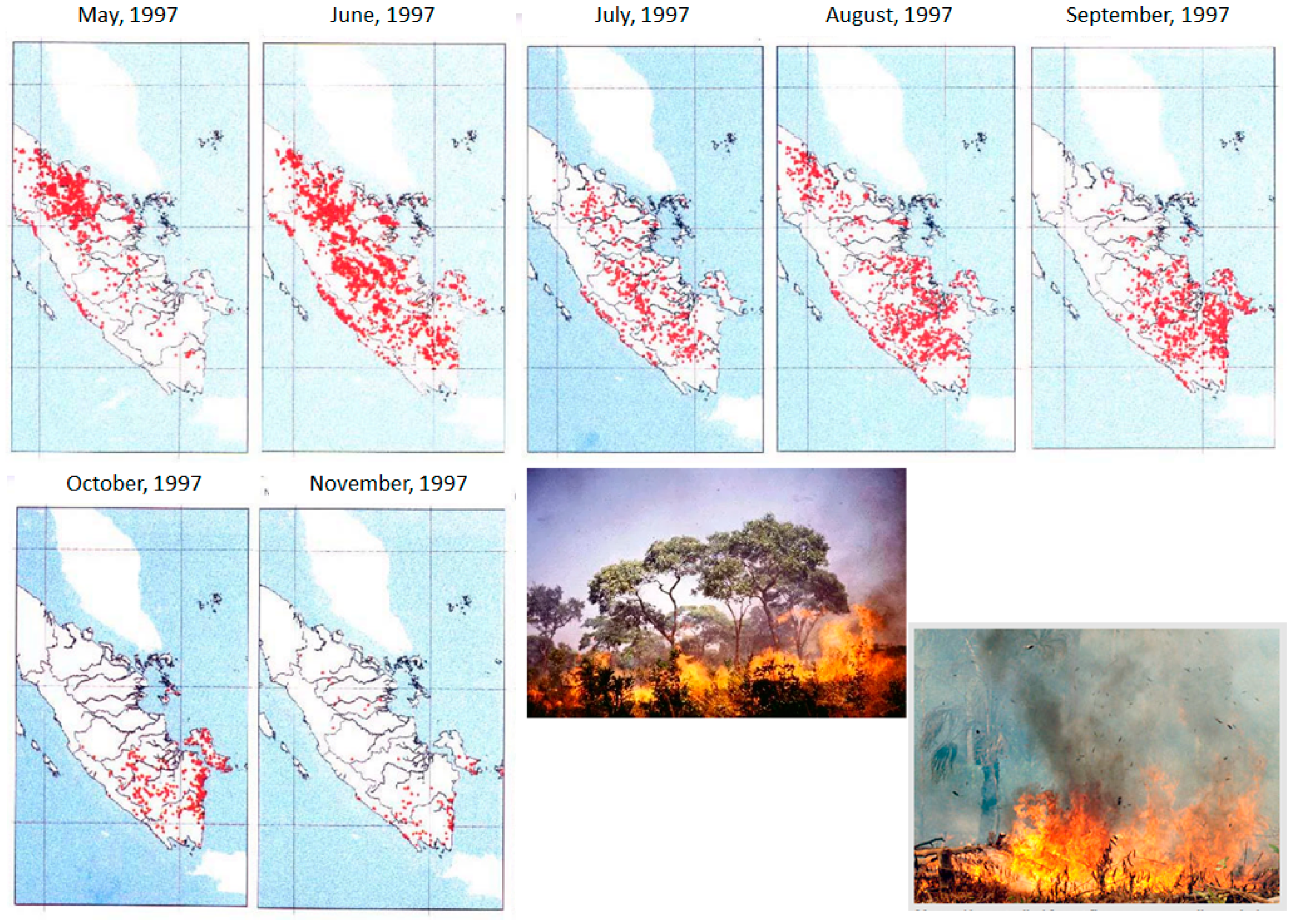
Figure 1. Distribution of hot spot in Sumatra 1997 [25].
Remotesensing 12 03700 g001
Figure 2. Location of the study area is in Sembilang National Park, Musi Banyuasin, South Sumatra Province, Indonesia. Selected remotely sensed image from Landsat 7 ETM+ (source from USGS) and administrative boundaries of the study area (source from Indonesian Geospatial Agency/BIG), and taken photograph from [68,69,70].
Remotesensing 12 03700 g002
Figure 3. Implementation of restoration program through natural regeneration assistance, enrichment planting, and seeding around Sembilang National Park [12,72,73].
Remotesensing 12 03700 g003
Figure 4. Methodology.
Remotesensing 12 03700 g004
Figure 5. Landsat imageries acquired in: (a) Landsat 5 (1989), (b) Landsat 5 (1998), (c) Landsat 7 ETM+ (2002), and (d) Landsat 8 OLI (2015).
Remotesensing 12 03700 g005
Figure 6. The distribution of training data.
Remotesensing 12 03700 g006
Figure 7. Land cover map as classification result in (a) 1989, (b) 1998, (c) 2002, (d) 2015.
Remotesensing 12 03700 g007
Figure 8. Land cover prediction map in (a) 2002 and (b) 2015.
Remotesensing 12 03700 g008
Figure 9. Prediction map for 2028.
Remotesensing 12 03700 g009
Figure 10. The probability matrix: (A) an interval of 9 years (1989–1998), (B) an interval of 4 years (1998–2002), and (C) an interval of 13 years (2002–2015).
Remotesensing 12 03700 g010
Figure 11. Area statistics (ha) of land cover class for the years 1989, 1998, 2002, 2015, and predicted 2028.
Remotesensing 12 03700 g011
Table 1. The Data Collected.
DatasetDate and ScaleSource
Landsat 517 May 1989 and 24 April 1998USGS
Landsat 7 ETM+30 June 2002USGS
Landsat 8 OLI26 June 2015USGS
The administrative boundaries1:50,000BIG
Table 2. Description of LULC classes.
ClassDefinition
Non-mangroveLand, built-up land, bare ground, roads, shrubs, vegetation, other habitats of mangrove.
MangroveA shrub or small tree that grows in coastal saline or brackish water.
WatersWater in certain areas, both static and dynamic, such as seas, rivers, lakes.
Table 3. The confusion matrix of support vector machine classification in 1989.
Classification SVMClassesTraining Data for Ground Check
MangroveNon-MangroveWaterTotalUser AccuracyError Commission
Mangrove4952049799.60.4
Non-mangrove053805381000
Water004054051000
Total4955404051440
Producer Accuracy10099.6100 OA99.8
Error omission00.40 Kappa0.9
Table 4. The confusion matrix of support vector machine classification in 1998.
Classification SVMClassesTraining Data for Ground Check
MangroveNon-MangroveWaterTotalUser AccuracyError Commission
Mangrove44613045997.12.8
Non-mangrove4649065397.40.6
Water043423461001.1
Total4506663421458
Producer Accuracy99.197.4100 OA98.5
Error omission0.92.50 Kappa0.9
Table 5. The confusion matric of support vector machine classification in 2002.
Classification SVMClassesTraining Data for Ground Check
MangroveNon-MangroveWaterTotalUser AccuracyError Commission
Mangrove53317155196.73.2
Non-mangrove7607061498.81.1
Water0635936598.31.6
Total5406303601530
Producer Accuracy98.796.399.7 OA97.9
Error omission1.33.60.3 Kappa0.9
Table 6. The confusion matric of support vector machine classification in 2015.
Classification SVMClassesTraining Data for Ground Check
MangroveNon-MangroveWaterTotalUser AccuracyError Commission
Mangrove5407054798.71.3
Non-mangrove062306231000
Water003603601000
Total5406303601530
Producer Accuracy10098.1100 OA99.5
Error omission01.10 Kappa0.9
Table 7. Area Land-use (years) 1989, 1998, 2002, and 2015.
ClassesArea (ha) and Percentages (%)1989199820022015
Mangrovearea (ha)58,145.536,847.455,548.360,697.5
(%)26.216.625.127.4
Non-mangrovearea (ha)53,265.473,327.458,419.151,965.8
(%)24.133.126.323.4
Waterarea (ha)109,886111,122107,329108,633
(%)49.650.248.549.1
Table 8. Transition Probability matrix in 1989–1998, 1998–2002 and 2002–2015.
PeriodLand CoverMangroveNon-MangroveWaters
1989–1998Mangrove0.60.30
Non-mangrove0.10.80.1
Water0.10.10.8
1998–2002Mangrove0.70.20.1
Non-mangrove0.70.30.1
Water0.10.20.7
2002–2015Mangrove0.80.10.1
Non-mangrove0.20.70.1
Water0.10.10.8
Table 9. Transition matrix area in 1989–1998, 1998–2002 and 2002–2015.
PeriodLand CoverMangroveNon-mangroveWaters
1989–1998Mangrove266,660142,7560
Non-mangrove84,159668,66261,928
Water141,08746,3331,047,267
1998–2002Mangrove446,200123,35547,648
Non-mangrove431,900202,64114,561
Water100,020208,094884,435
2002–2015Mangrove547,05099,30028,066
Non-mangrove128,752414,68633,960
Water87,208104,8041,015,025
Table 10. Land cover area of prediction map in 2002 and 2015.
ClassesArea (ha) and Percentages (%)Prediction (2002)Prediction (2015)
Mangrovearea (ha)42,224.186,245.2
(%)19.138.9
Non-mangrovearea (ha)77,012.647,087.1
(%)3421.2
Waterarea (ha)10,059.987,964.2
(%)46.139.7
Table 11. Kappa Index Agreement in prediction years 2002 and 2015.
Kappa Index of Agreement2002 (Prediction)2015 (Prediction)
Kno0.70.7
Klocation0.80.8
KlocationStrata0.80.8
Kstandard0.70.7
Table 12. Land cover change prediction.
ClassesArea (in ha) and Percentages (%)19891998200220152028
Mangrovearea (ha)58,145.536,847.455,548.360,697.568,672.3
(%)26.216.625.127.431
Non-mangrovearea (ha)53,265.473,327.458,419.151,965.855,691.1
(%)24.133.126.323.425.1
Waterarea (ha)109,886111,122107,329108,63396,933.3
(%)49.650.248.549.143.8
Table 13. The suitability time of Landsat imagery and tidal height.
Landsat ImageryTidal Height
Remotesensing 12 03700 i001 Remotesensing 12 03700 i002
17 May 198917 May 1989
Remotesensing 12 03700 i003 Remotesensing 12 03700 i004
24 April 199824 April 1998
Remotesensing 12 03700 i005 Remotesensing 12 03700 i006
30 June 200230 June 2002
Remotesensing 12 03700 i007 Remotesensing 12 03700 i008
26 June 201526 June 2015
Table 14. The classification accuracy.
YearsOverall AccuracyKappa StatisticsMangrove User AccuracyMangrove Producer Accuracy
198999.80.999.6100
199898.50.997.299.1
200297.90.996.798.7
201599.50.998.7100
Publisher’s Note: MDPI stays neutral with regard to jurisdictional claims in published maps and institutional affiliations.