


Abstract
In this study, global spatial autocorrelation, local spatial autocorrelation, Spearman correlation analysis, gray correlation analysis, entropy weight method, and the gravity model were used to analyze the spatiotemporal variation and environment-urban-economy-associated factors of air quality of 31 provinces in China during 2015~2022. From 2015 to 2022, the Air Quality Index (AQI) exhibited a downward trend in 30 out of 31 Chinese provinces, with the exception of Shaanxi Province. Concurrently, the annual average concentrations of PM2.5, PM10, SO2, NO2, and CO declined across the study period. High-high clusters and low-high outliers were observed in northern China, whereas low-low clusters and high-low outliers were distributed in southern China. Twelve provinces (38.7%) showed positive correlation (0.095~0.95), 18 provinces (58.1%) showed negative correlation (−0.76~0.095), and only Anhui showed no correlation between AQI and O3. The comprehensive AQI quality presented a dual-core model in Sichuan (in the southwest) and Henan (in the central part) of China, while the comprehensive AQI improvement rate presented a single-core model in Jiangsu in the east of China. The gravity models incorporating AQI and GDP revealed that both air quality and economic performance improved over the study period. The spatial pattern of pollution evolved from a multi-core structure to a non-core structure, whereas the pattern of economic growth transitioned from a non-core structure to a dual-core structure, with the Beijing-Tianjin-Hebei region and the Yangtze River Delta emerging as the primary urban agglomerations.
1. Introduction
With the rapid development of China’s economy and the rapid advancement of urbanization and industrialization, air pollution has long been increasingly serious, inflicting huge health damage and social losses on the public [1,2,3,4]. Research data indicate that long-term exposure to highly polluted air increases human health risks, giving rise to adverse effects on the cardiovascular system, respiratory system, lungs, and other aspects [5,6,7,8]. To curb the further deterioration of air pollution, safeguard public health, and alleviate the impacts of climate change, China’s air pollution control policies have evolved substantially over the past few decades. Notably, policy implementation has been strengthened considerably, transitioning from lax enforcement to rigorous execution [9,10]. Industrial activities release heavy metals, causing global air pollution. Contamination was assessed via the geoaccumulation index and enrichment factors. Industrial, agricultural, and mining emissions raise metal levels, damaging cells and triggering carcinogenic risks [11]. Atmospheric Cd deposition flux in China rose slightly during 2006–2015 versus 1999–2006, yet regional research ignoring spatial heterogeneity is lacking. Southern China recorded a higher flux of 1.05 mg·(m2·a)−1 than the northern 0.89 mg·(m2·a)−1, but unfiltered mining and industrial sites may overestimate the flux [12]. A series of air pollution prevention and control measures, such as the “Action Plan for Air Pollution Prevention and Control” and the “Three-year Action Plan for Winning the Blue Sky Defense”, have achieved remarkable results in air pollution control [13,14,15,16]. From 2013 to 2022, the concentration of fine particulate matter (PM2.5) in 74 key Chinese cities continued to decline from 72 μg/m3 to 30 μg/m3, with a cumulative decrease of 58%. Nevertheless, 25% of Chinese cities still have PM2.5 concentrations exceeding 35 μg/m3, thus failing to meet the National Ambient Air Quality Standards [2,17,18].
The improvement of air quality is a complex dynamic process, which is jointly affected by environmental factors, human activities, economic development, industrial structure, meteorological conditions, and other factors, with characteristics of “scarce effective data and poor information” [19,20,21,22]. Domestic and foreign scholars have conducted extensive research on the improvement of air pollution and its associated factors [23,24,25,26]. Liu et al. [27] used exploratory spatial data analysis and the Spatial Durbin Model (SDM) to quantitatively estimate the contribution and spatial spillover of different natural and human factors to air quality. The results showed that urbanization, urban population agglomeration, and industrialization had a significant positive impact on AQI, but the amount of urban land, per capita GDP, altitude, and relative humidity had no significant impact. Xu et al. [28] employed social network analysis, extended production theory decomposition analysis, and the proposed spatiotemporal decoupling model. They explored the network structure and associated factors of PM2.5 concentration as well as its decoupling relationship with Fiscal Environmental Expenditure. The study revealed that per capita GDP and the Potential Intensity of PM2.5 and FEE were the most influential factors in reducing PM2.5 concentration. Wang et al. [29] combined the Relaxation-Based Measure (SBM) model, the Global Malmquist-Luenberger (GML) productivity index, and the panel Tobit model to study the regional differences, dynamic evolution, and influencing factors of provincial air pollution emission efficiency in China during 2006~2015, and the results showed that China’s provincial air pollution total factor emission efficiency was significantly positively correlated with economic development level, industrial structure optimization, technological innovation, and foreign direct investment (FDI), and significantly negatively correlated with energy consumption structure. Numerous studies have demonstrated that air quality improvement is closely associated with economic development potential. Therefore, clarifying the core driving force of air quality improvement is a necessary prerequisite for achieving high-quality economic and social development [30,31,32,33].
In order to better understand the associated factors of air pollution, many studies focus on using numerical analysis methods and related models to study the spatiotemporal differentiation characteristics and associated factors of air quality in a certain city or a certain district, providing a basis for environmental management and government decision-making [34,35,36,37,38]. Fan et al. [39] explored the coupling relationship between urbanization and air quality in Shandong Province from 2014 to 2017 by using global principal component analysis, the harmony degree model, the coupled coordination degree model, and the geographic information system (GIS). The results showed that in Shandong Province, as China’s economy shifted from the stage of high-speed growth to the stage of high-quality development, urbanization and the coupling coordination degree of air quality index and pollutants gradually tended towards a high level of coordination. Therefore, in the process of urban development, highly coordinated cities should play a more leading role in the surrounding areas, and cities with lagging urbanization need to strengthen environmental protection policies. Jiang et al. [40] analyzed and quantified the factors affecting air pollution based on air pollution observation, as well as synchronous meteorological and socio-economic data, of 103 cities during 2014~2019. The results of the Spatial Durbin Model (SDM) indicate that air pollution exerts a significant spatial spillover effect within the Yellow River Basin at the basin scale. Government technology expenditure, GDP per capita, population density, annual wind speed and relative humidity all have significant overall negative effects on the air quality index. Green coverage, proportion of secondary industry and air temperature all have significant positive total effects. Zhang et al. [41] investigated the spatiotemporal dynamics of air quality in Shandong Province from 2016 to 2022, and found that affected by industrial activities and geographical characteristics, the air quality of coastal cities is better than that of inland areas, and the optimization and transformation of industrial structure plays a crucial role in improving air environmental quality; stringent policies and technological advances can lead to significant improvements in air quality. However, current studies mainly focus on using a certain type of method or model to study the improvement of air quality in a single city or a single region, and there are insufficient studies on the evolution of air quality and its associated factors in China. Therefore, based on the data system of 31 provinces of China, this study studied the spatiotemporal differentiation characteristics of China’s overall air quality and the interaction between air quality and environmental, urban and economic associated factors, which is helpful for formulating targeted policies and achieving the win-win goal of China’s regional economic development and air environmental protection [42,43,44,45]. It is of urgent and important significance to achieve high-quality development and sustainable development [46].
In this study, the spatiotemporal variation of air quality and its environment-urban-economy-associated factors of 31 provinces of China during 2015~2022 were analyzed using global spatial autocorrelation, local spatial autocorrelation, Spearman correlation analysis, grey correlation analysis, the entropy weight method, and the gravity model. This study aims to investigate the synergistic effects between air pollution and economic growth across Chinese provinces and regions, explore the regional disparities inherent in the relationship between economic development and environmental change, and propose targeted recommendations for the coordinated and sustainable development of China’s regions.
2. Experimental Methods
2.1. Research Areas and Data Sources
The research area of 31 provinces was represented by 27 provincial capital cities and four municipalities. The geographical locations are shown in Figure 1, and the city and province numbers are shown in Table 1. China plays a pivotal role in the global landscape. In the process of rapid development, China attaches great importance to the win-win situation of environmental protection and economic development and insists on promoting green and low-carbon economic and social development to achieve high-quality development. The air pollution caused by China’s development in recent decades is also worthy of attention. However, there are few studies on the interaction of air pollution among different provinces, which lack in-depth exploration. Therefore, based on the inter-provincial network, this paper carried out an analysis of the spatiotemporal variation and associated factors of air quality of 31 provinces of China during 2015~2022.
Figure 1.
Schematic diagram of geographical location for 31 provinces. Guiyang (GY), Fuzhou (FZ), Guangzhou (GZ), Haikou (HK), Chengdu (CD), Wuhan (WH), Changsha (CS), Nanchang (NC), Hefei (HF), Nanjing (NJ), Hangzhou (HZ), Xining (XN), Shijiazhuang (SJZ), Zhengzhou (ZZ), Xi’an (XA), Taiyuan (TY), Jinan (JN), Lanzhou (LZ), Shenyang (SY), Changchun (CC), Harbin (HEB), Kunming (KM), Hohhot (HHHT), Nanning (NN), Lhasa (LS), Yinchuan (YC), Urumqi (WLMQ), Beijing (BJ), Tianjin (TJ), Shanghai (SH), Chongqing (CQ).
Table 1.
The 31 provinces and related information on the research areas.
Air quality data (PM2.5, PM10, SO2, NO2, CO, O3 concentrations, and AQI) are all derived from urban ambient air quality information released by the Ministry of Environmental Protection (https://www.mee.gov.cn/, accessed on 1 January 2024). The data on pollutant emission, urban development, and economic growth come from China Urban Statistical Yearbook (https://www.stats.gov.cn/sj/ndsj/, accessed on 1 January 2024), China Urban Construction Statistical Yearbook (https://www.mohurd.gov.cn/, accessed on 1 January 2024), China Statistical Abstract (https://www.stats.gov.cn/, accessed on 1 January 2024), Environmental Statistics Yearbook of China (http://60.16.24.131/, accessed on 1 January 2024), and Statistical Yearbooks of 31 cities (https://www.stats.gov.cn/, accessed on 1 January 2024). Environmental pollution emission factors include industrial nitrogen oxide emissions (X1), industrial sulfur dioxide emissions (X2), industrial wastewater emissions (X3), and industrial powder (smoke) dust emissions (X4). Urban development index factors include permanent resident population (X5), urban per capita green park area (X6), urban green coverage area (X7), and urban population density (X8). Economic growth index factors include the added value of the primary industry (X9), the added value of the secondary industry (X10), the added value of the tertiary industry (X11), GDP (X12), and per capita GDP (X13).
2.2. Research Methods
2.2.1. Global Spatial Autocorrelation
Global Moran’s I is an exploratory spatial analysis index used to examine the problem of low spatial correlation and agglomeration. It reflects the degree of similarity between each regional unit and its neighboring units across the entire study area and is employed to identify whether the spatial distribution of geographic features or attributes exhibits clustering patterns [47]. The global Moran’s I is calculated as follows:
where n represents the total number of regional units in the study area, Xi represents the X variable value of the provincial capital city i studied by the regional unit, and Wij represents the element value of the spatial weight matrix, representing the spatial adjacency characteristics. If i and j share a boundary line in space, Wij = 1; otherwise, Wij = 0. Taking the calculation of AQI global autocorrelation as an example, Xi represents the AQI value of the provincial capital city i, Xj represents the AQI value of the provincial capital city j, i ≠ j, i/j = 1, 2, 3, … 31. The calculation process of the six major pollutants is consistent with the calculation process of the AQI global autocorrelation.
Since Moran’s I is the estimated value of the coefficient of the spatial autocorrelation regression equation, its value range is [−1, 1]. When Moran’s I is greater than 0, it indicates a positive correlation, and when the value is close to 1, it indicates that similar attributes cluster together. A value below 0 denotes a negative spatial correlation; a value approaching −1 signifies the clustering of dissimilar attributes. A value near 0 indicates a random distribution of the attribute or an absence of spatial autocorrelation.
2.2.2. Local Spatial Autocorrelation
Local autocorrelation is primarily employed to analyze the spatial agglomeration and correlation intensity of local spatial units and to further characterize their spatial autocorrelation with adjacent units. The commonly used indicator is the Local Moran’s I Index, which can reveal the local clustering and outliers in spatial data, with four types of spatial correlation: two positive correlation-spatial correlation (High-High Cluster and Low-Low Cluster) and two negative correlation-spatial outliers (High-Low Outlier and Low-High Outlier). The calculation formula is as follows:
where Ii represents the local Moran’s I of spatial position i. Taking the calculation of AQI local autocorrelation as an example, Xi represents the AQI value of provincial capital city i, Xj represents the AQI value of provincial capital city j, i ≠ j, i/j = 1, 2, 3, … 31. The calculation process of the six major pollutants is consistent with the calculation process of the AQI local autocorrelation. Ii > 0 and the significance test indicates that regions with the same or similar attributes are close to each other in space; that is, they are represented as “high-high” or “low-low” clusters. Ii < 0 and the significance test indicates that regions with large attribute differences are close to each other in space; that is, they are represented as “high-low” or “low-high” outliers.
2.2.3. Spearman Correlation Analysis
Spearman’s correlation coefficient is a nonparametric statistical measure used to evaluate the monotonic relationship between two variables. Spearman correlation analysis was applied to quantify the associations between AQI and individual pollutant indices, environmental pollutant emission factors, urban development indicators, and economic indicators [48]. The calculation process is as follows:
where n represents the sample size, n = 31, X and Y are defined as two sets of data, Xij and Yij represent the grades of these two sets of data, respectively, and d represents the grade difference between Xij and Yij after ordering the samples from small to large. When calculating the correlation of AQI-environmental pollutant emission factors in 2022, Xij represents the AQI value in 2022 of the i-th province, and Yij represents the industrial nitrogen oxide emissions, industrial sulfur dioxide emissions, industrial wastewater emissions, and industrial powder (smoke) dust emissions in 2022 of the i-th province, respectively. The correlation calculation process of other indicators is consistent with the correlation calculation process of AQI-environmental pollutant emission factors.
2.2.4. Grey Correlation Analysis
Grey correlation analysis is a method that quantifies the degree of correlation among factors through mathematical computation of selected variables and identifies their relationships based on the similarity of their numerical change curves [49]. Grey correlation analysis was employed to quantify the correlations between AQI and environmental pollution emission factors, urban development factors, and economic growth factors. The calculation process is as follows:
where ∆i(k) represents the variance sequence. In order to make a comparison between indicators, dimensionless processing is carried out by the initial value method, where ρ is the resolution coefficient, ρ is usually 0.5, and the correlation degree R is the quantitative relationship of the correlation degree between the comparison series and the reference series. When calculating the correlation degree of AQI-environmental pollution emissions, X0 is used as the reference sequence, X0(k) represents the AQI value in different years, and Xi represents the pollutant emission successively in different years: i = 1, 2, 3, 4, and so on. In this calculation, X1 is the industrial nitrogen oxide emissions, X2 is the industrial sulfur dioxide emissions, X3 is the industrial wastewater emissions, and X4 is the industrial powder (smoke) dust emissions. The procedure for calculating the correlation degree among other indicators is consistent with that employed for the correlation degree between AQI and pollutant emissions.
2.2.5. Entropy Weight Method
The entropy weight method is an objective weighting approach employed to determine indicator weights, and it is widely utilized in multi-index comprehensive evaluation. Its core idea is to use information entropy to measure the degree of dispersion of each indicator, so as to determine its weight in the comprehensive evaluation. The entropy weight method was applied to assess the weights of environmental pollution emission factors, urban development factors, and economic growth factors in influencing air quality. The calculation process is as follows:
where Ej represents information entropy, Ptij represents the proportion of the value of the i sample of the j-th index in the index, and Xtij represents the value of the j index of the i sample of the year t (t = 1, 2, … 8; i = 1, 2, … 31; j = 1, 2, … 13). When the original data is standardized, Ytij represents the standardized value, and Wj represents the weight. When calculating the environmental pollutant emission weight, when t = 1, 2, … 8, it means 2015, 2016, … 2022, respectively. When i = 1, 2, … 31, it represents the 31 provinces, respectively. When j = 1, 2, 3, 4, they represent the indicators of industrial nitrogen oxide emissions, industrial sulfur dioxide emissions, industrial wastewater discharge, and industrial dust (smoke) emissions, respectively. The weight calculation procedure for other indicators is consistent with that applied to environmental pollutant emissions.
2.2.6. Gravity Model
The gravity model is a fundamental model for predicting the interaction between objects. The gravity between any two objects is proportional to their masses and inversely proportional to their distance. The gravity model is used to calculate the interactions of AQI and the interactions of GDP among 31 provinces. The gravity model employed in this study merely quantifies the intensity of spatial interactions based on spatial proximity and AQI similarity, without connoting any genuine physical gravitational attraction or causal linkage. The calculation process is as follows:
where F represents the gravity between the two provinces, Q represents the size of the two provinces, d represents the distance between the two provinces, and a = 1. When calculating the AQI interaction between two provinces, Q1 and Q2 represent the AQI values of the two provinces, respectively, and d represents the geometric center distance between the two provinces. Similarly, when calculating the GDP interaction between two provinces, Q1 and Q2 represent the GDP values of the two provinces, respectively, and d represents the geometric center distance between the two provinces.
3. Results and Discussion
3.1. Spatiotemporal Variation of Air Quality
Figure 2 depicts the interannual variations in AQI across 31 provincial-level regions of China from 2015 to 2022. On the whole, the air quality has improved, and AQI shows a downward trend. In 2015, the order of AQI values of provinces is Henan (125.94) > Hebei (117.29) > Shandong (115.31) > Beijing (107.29) > Liaoning (96.35) > Heilongjiang (94.69) > Tianjin (94.17) > Hubei (93.75) > Xinjiang (91.63) > Sichuan (91.15) > Jilin (88.96) > Anhui (88.33) > Shaanxi (88.04) > Gansu (84.04) > Shanxi (83.13) > Hunan (82.29) > Ningxia (81.13) > Qinghai (77.67) > Jiangsu (77.60) > Zhejiang (77.40) > Chongqing (77.08) > Inner Mongolia (75.54) > Shanghai (72.50) > Jiangxi (62.71) > Guangxi (60.96) > Guangdong (58.65) > Guizhou (55.42) > Tibet (54.08) > Yunnan (53.00) > Fujian (52.83) > Hainan (39.67). In 2022, the order of AQI values of provinces is Shaanxi (93.09) > Henan (73.54) > Sichuan (71.98) > Hebei (69.90) > Xinjiang (68.44) > Shanxi (67.60) > Hunan (62.40) > Shandong (61.04) > Gansu (60.79) > Heilongjiang (60.63) > Hubei (58.54) > Tianjin (58.44) > Ningxia (58.21)> Anhui (56.83) > Qinghai (54.08) > Chongqing (53.33) > Liaoning (53.13) > Jiangxi (52.83) > Beijing (52.29) > Zhejiang (50.88) > Jiangsu (50.71) > Inner Mongolia (50.33) > Guangdong (48.28) > Jilin (48.08) > Shanghai (42.27) > Guangxi (42.08) > Fujian (38.52) > Tibet (35.86) > Hainan(35.68) > Yunnan (35.65) > Guizhou (34.75). From 2015 to 2022, the order of air quality improvement in provinces is Beijing (51.26%) > Shandong (47.06%) > Jilin (45.95%) > Liaoning (44.86%) > Shanghai (41.70%) > Henan (41.60%) > Hebei (40.41%) > Tianjin (37.94%) > Hubei (37.56%) > Guizhou (37.92%) > Heilongjiang (35.97%) > Anhui (35.66%) > Jiangsu (34.66%) > Zhejiang (34.27%) > Tibet (33.70%) > Inner Mongolia (33.37%) > Yunnan (32.73%) > Guangxi (30.96%) > Chongqing (30.81%) > Qinghai (30.36%) > Ningxia (28.25%) > Gansu (27.66%) > Fujian (27.10%) > Xinjiang (25.31%) > Hunan (24.18%) > Sichuan (21.03%) > Shanxi (18.67%) > Guangdong (17.67%) > Jiangxi (15.75%) > Hainan (10.06%) > Shaanxi (−5.74%). In terms of years, the average AQI value of provinces showed a downward trend from 2015 to 2022, and the overall air quality was significantly improved. Only the AQI value of Shaanxi increased, and the air quality deteriorated. In 2015, only one province in Hainan reached Grade I (AQI < 50). In 2022, nine provinces in Jilin, Shanghai, Guizhou, Tibet, Yunnan, Guangxi, Fujian, Guangdong, and Hainan reached Grade I, and the AQI value of 31 provinces decreased from 81.24 to 54.84. Regionally, the spatial distribution of AQI is generally characterized by low in the southeast and high in the northwest, and low in the coastal areas and high in the inland areas. Air quality in southern China is superior to that in northern China, yet the improvement rate of air quality in the north is higher than that in the south. All provinces with an AQI reduction exceeding 40% are located in northern China. Meanwhile, air quality improvement rates in southwestern, southern, eastern, and northeastern China are higher than those in northwestern, northern, and central China. In 2022, air quality across all of southern China attained Grade I, whereas air quality in central China was poorer relative to other regions. The reason may be that the economic development of some provinces located in the central region depends on traditional heavy industries such as coal, the chemical industry, and steel [50]. The results reveal an overall downward trend in AQI throughout the pandemic period, with a substantially more prominent improvement in air quality observed following the outbreak. This analysis compares the average AQI and pollutant concentrations between 2015–2019 and 2020–2022, where the enhanced air quality can be primarily attributed to the curtailment of anthropogenic activities and industrial production. Consequently, industrial emissions have emerged as the primary factor influencing local AQI values. The relatively lower air quality index in southern coastal regions may be associated with multiple factors, including their economic development model, environmental protection investment, meteorological conditions, and provincial development levels.
Figure 2.
Annual AQI change for 31 provinces of China during 2015~2022. (a) 2015, (b) 2016, (c) 2017, (d) 2018, (e) 2019, (f) 2020, (g) 2021, (h) 2022.
From 2015 to 2022, the annual average concentrations of the six primary air pollutants exhibited provincially divergent trends across China: PM2.5, PM10, SO2, NO2, and CO generally declined, while O3 increased. PM2.5 concentrations showed an overall decrease of 36.59%, dropping from 57.14 μg/m3 to 36.23 μg/m3. In 2015, Henan had the highest concentration (95.75 μg/m3), and Hainan had the lowest (22.08 μg/m3). Tibet (64.67%) and Beijing (60.00%) achieved the largest improvements, though Shaanxi saw a 19.44% rise. PM10 concentrations fell by 43.58% on average, from 97.42 μg/m3 to 54.97 μg/m3. Henan topped the 2015 rankings (169.33 μg/m3), but by 2022, Shaanxi led (89.58 μg/m3). Tibet showed the most significant improvement (69.34%), followed by Jilin (55.27%) and Shandong (54.11%). SO2 recorded the sharpest decline at 67.30%, with average concentrations dropping from 26.07 μg/m3 to 8.52 μg/m3. Shanxi had the highest concentration in 2015 (71.17 μg/m3), while Qinghai led in 2022 (17.33 μg/m3). Shanxi (83.02%) and Hebei (82.92%) drove this reduction with the largest improvements. NO2 concentrations decreased by 34.86% overall, from 41.86 μg/m3 to 27.22 μg/m3. Henan ranked highest in 2015 (57.50 μg/m3), and Shanxi took the lead in 2022 (40.00 μg/m3). Beijing achieved the biggest improvement (54.50%), followed by Henan (52.46%) and Fujian (52.28%). CO concentrations declined year by year, falling 44.32% from 1.65 mg/m3 in 2015 to 0.92 mg/m3 in 2022. Hebei had the highest concentration in 2015 (2.70 mg/m3), while Qinghai led in 2022 (1.31 mg/m3). Beijing (65.08%) and Hebei (59.57%) showed the most notable improvements. In contrast, O3 concentrations rose by 10.18% overall, with a trend of initial increase (116.09 μg/m3 in 2015 to 133.56 μg/m3 in 2019) followed by a slight decrease to 127.91 μg/m3 in 2022. Beijing had the highest concentration in 2015 (147.83 μg/m3), but Guangdong took the top spot in 2022 (154.50 μg/m3). Only Jilin saw an improvement (16.87%), while Anhui experienced the largest increase (−48.91%). Distinct regional disparities were observed across all pollutants: northern provinces generally exhibited higher initial pollutant concentrations yet achieved substantial improvements, whereas southern regions maintained comparatively lower baseline levels. In contrast to other provinces, Shaanxi implemented PM2.5 and SO2 emission reduction policies with a later timetable and weaker enforcement intensity. Moreover, we observed a pronounced upward trend in O3 concentrations across the province, which directly accounted for the increase in AQI. The contrasting trend of O3, rising amid other pollutants’ decline, highlights emerging challenges in air quality management, in Figures S1–S6 and Supplementary Text S1.
As shown in Figures S7–S12, from 2015 to 2022, monthly average concentrations of PM2.5, PM10, SO2, NO2, and CO across Chinese provinces showed a “V” shape, while O3 displayed an inverted “V” pattern. For PM2.5, Tibet (69.43%) and Beijing (63.30%) achieved the largest improvements in monthly concentrations, with Shaanxi being the only province with a decline (−10.05%). PM10 improvements were led by Hunan (69.34%) and Ningxia (55.27%), though Anhui showed the smallest gain (26.19%). SO2 saw the most dramatic progress, led by Shanxi (83.02%), Hebei (82.92%), and Beijing (79.14%), with over 75% improvement in nine provinces. NO2 improvements were headed by Beijing (54.50%), Henan (52.46%), and Fujian (52.28%), while Shanxi (−5.03%) regressed. CO improvements were greatest in Beijing (65.08%), Hebei (59.57%), and Inner Mongolia (58.58%), with Hainan (20.00%) showing the least progress. In contrast, O3 worsened in most provinces: only Jilin (16.87%) improved, while Anhui (−48.97%) and Xinjiang (−41.31%) saw the sharpest increases. These trends highlight regional disparities, with northern provinces often showing larger improvements for traditional pollutants, while O3 remains a growing challenge, as shown in Supplementary Text S1.
The seasonal variations in concentrations of the six primary pollutants across spring, summer, autumn, and winter are presented in Figures S13–S16. The seasonal average value of PM2.5 in the six major pollutants was 29.02 μg/m3~61.15 μg/m3, the seasonal average value of PM10 was 57.86 μg/m3~94.14 μg/m3, the seasonal average value of SO2 was 9.74 μg/m3~19.14 μg/m3, the seasonal average value of NO2 was 29.11 μg/m3~47.10 μg/m3, the seasonal average value of CO was 0.95 mg/m3~1.76 mg/m3, and the seasonal average value of O3 was 78.76 μg/m3~165.01 μg/m3. PM2.5, PM10, SO2, NO2, and CO were characterized by a “high in spring and winter, low in summer and autumn” trend. However, O3 showed a “high in summer and autumn, low in spring and winter” trend. Those findings of PM2.5, PM10, SO2, NO2, and CO in spring, summer, autumn, and winter should not be generalized to the entire province.
3.2. Spatial Autocorrelation Analysis of Air Quality
Autocorrelation analysis was performed to clarify the spatial correlation and clustering characteristics of air pollution across regions, with the results presented in Table 2. From the point of view of years, except for a few years, the p-value of the global Moran’s I was basically below 5%, which passed the significance test, and the calculation results have obvious statistical significance. From the perspective of air quality indicators, except that the significance test of NO2 for Moran’s I had the worst effect between 2015 and 2022, with a non-significant p-value, the p-values of the remaining indicators were below 5%, and their results were also statistically significant. At the same time, the global Moran’s I was greater than 0, which indicates that there was a significant global positive correlation in the relevant air quality indicators during 2015~2022. Among them, the Moran’s I values of AQI, PM2.5, SO2, and CO showed undulating changes; that is, they first decreased, then increased, and then decreased again. The Moran’s I value of O3 first increased and then decreased, and tended to stabilize, and the correlation first increased and then weakened. The Moran’s I index for PM10 remained consistently high, exhibiting a stronger positive spatial correlation and greater stability compared with other indicators. In 2015, the annual average PM2.5 concentrations in Henan, Hebei, and Shandong provinces were more than twice the permissible limit of 35 μg/m3, while by 2022, only a handful of provinces exceeded this threshold. Furthermore, a considerable number of provinces surpassed the 8-h O3 standard of 160 μg/m3 in the summer months.
Table 2.
Moran’s I index of air quality for global spatial autocorrelation during 2015~2022.
To further investigate the magnitude and significance of spatial disparities across regions, local spatial autocorrelation analysis was conducted for various air quality indicators. As illustrated in Figure 3, a low-low cluster—representing a cold spot with favorable air quality—was identified in southern China, primarily concentrated in Yunnan, Guangxi, and Fujian provinces. Both low-high and high-low outliers exhibited a scattered distribution. Notably, Inner Mongolia displayed a low-high outlier pattern, which evolved from an insignificant state to a high-high cluster, and subsequently to a low-high outlier over the period 2015–2022. “High-low” outliers were mainly distributed in Sichuan and Hunan. The “high-high” cluster was mainly distributed in the geographically northern region, presenting as a “hot spot” region with poor air quality, which was a feature of concentrated distribution of pollution. The relevant provinces had a high AQI and were surrounded by provinces with high AQI values in the surrounding areas. The agglomeration area expanded initially and then contracted annually. In 2015, the agglomeration state was concentrated in Beijing, Tianjin, Henan, Shanxi, Shandong, and Hebei. In 2022, it was mainly distributed in Gansu, Ningxia, Shaanxi, Shanxi, Henan, and Hubei. From 2019 to 2022, the “high-high” cluster was distributed in North China and successively in East China, Central China, and Northwest China, showing a trend of shifting from the east to the central and western regions.
Figure 3.
Local spatial autocorrelation for AQI of China during 2015~2022. (a) 2015, (b) 2016, (c) 2017, (d) 2018, (e) 2019, (f) 2020, (g) 2021, (h) 2022.
Figures S17–S22 present the local spatial autocorrelation analysis for the six primary pollutants. For PM2.5, “low-low” clusters, similar to AQI, were concentrated in Yunnan and Guangxi. “Low-high” outliers appeared in Inner Mongolia (2017, 2021, 2022); “High-low” outliers were intermittent in Xinjiang and Sichuan; “High-high” clusters shifted west, from Beijing, Tianjin, Hebei, Shandong, Henan, and Anhui (2015) to Gansu, Shaanxi, Chongqing, Hubei, Shanxi, and Henan (2022). PM10’s “low-low” clusters shrank from southern provinces (Yunnan, Guizhou, Guangxi, Hunan, Jiangxi, Zhejiang, and Fujian in 2015) to Yunnan, Guizhou, and Guangxi (2022). “Low-high” outliers appeared intermittently in Liaoning (2017), Beijing (2021), and Inner Mongolia (2022). “High-high” clusters, which were northern-focused, shifted from Inner Mongolia, Beijing, Tianjin, Hebei, Shandong, Shanxi, Shaanxi, and Henan (2015) to Gansu, Shaanxi, Shanxi, Henan, Hebei, and Shandong (2022). SO2’s “low-low” clusters declined from Yunnan, Hunan, Jiangxi, Zhejiang, and Fujian (2015) to only Jiangxi and Zhejiang (2020–2022). “Low-high” outliers appeared in Xinjiang (2021–2022); there were no “high-low” outliers. “High-high” clusters stayed in Inner Mongolia, Jilin, Hebei, and Henan (2015) and Inner Mongolia, Jilin, and Henan (2022). NO2 differed, with “low-low” clusters in Yunnan and Guangxi. “Low-high” outliers were scattered in Anhui (2015), Ningxia (2018), and Inner Mongolia (2021). “High-low” outliers were in Sichuan (2015) and Guangdong (2021–2022). “High-high” clusters expanded from Henan (2015) to Inner Mongolia, Gansu, Ningxia, Shaanxi, Shanxi, and Henan (2022). CO’s “low-low” clusters shrank from Yunnan, Guizhou, Guangxi, Hunan, Jiangxi, Fujian, and Zhejiang (2015) to Yunnan (2022). There were “low-high” outliers in Inner Mongolia (2017, 2022) and “high-low” outliers only in Guangxi (2022). “High-high” clusters fluctuated: in Inner Mongolia, Shanxi, Hebei, Beijing, Tianjin, and Henan (2015); in Henan (2018); in Hebei and Henan (2022). O3’s “low-low” clusters, initially unclear, shifted to the southwest, then the northwest, then Heilongjiang and Jilin (2022). “Low-high” outliers were rare (Anhui 2015; Fujian 2021; none in 2022). “High-low” outliers stabilized in Sichuan (2019–2022). “High-high” clusters expanded from Henan and Jiangsu (2015) to Hebei, Shandong, Henan, Anhui, Jiangsu, Jiangxi, and Fujian (2022), as shown in Supplementary Text S2.
3.3. Correlation Analysis Between AQI and Pollutant or Environment-Urban-Economy-Associated Factors
3.3.1. Spearman Correlation Analysis Between AQI and Six Major Pollutants
According to the relevant data of 31 provinces during 2015~2022, the Spearman correlation coefficient of AQI-pollutant was calculated, as shown in Figure 4. It revealed the interrelation among pollutants AQI, PM2.5, PM10, SO2, NO2, CO, and O3 and revealed the potential common source or similar diffusion characteristics. There was a significant positive correlation between AQI and PM2.5, PM10, SO2, NO2, and CO in most provinces (0.650~1.000) and the sources of pollutants had certain homology, but the correlation between some indicators in some provinces was weak: the correlations between PM2.5 and NO2 and between PM2.5 and CO in Jiangxi was weak, both of which were 0.19; the correlations between AQI and NO2, PM2.5, and PM10 in Anhui were 0.330, 0.360, and 0.330, respectively. The correlations between AQI and SO2, NO2, and CO in Shaanxi were 0.380, 0.330, and 0.310, respectively, and the correlations between PM2.5 and SO2, NO2, and CO were 0.310, 0.400, and 0.240, respectively. The increase in O3 concentrations accompanied by the reduction in NO2 is consistent with the well-established VOC-limited or transition regime that characterizes most urban areas across China. Diminished NO2 levels weaken the nocturnal titration effect on ozone, consequently fostering higher daytime O3 accumulation. The negative correlation between AQI and O3 observed in 18 provinces, including Yunnan and Guizhou, demonstrates that while NO2 reductions have enhanced overall air quality, a severe ozone pollution challenge has concurrently emerged.
Figure 4.
Spearman correlation coefficients for AQI and PM2.5, PM10, SO2, NO2, CO, and O3 in China during 2015~2022. (a1) Guizhou, (a2) Fujian, (a3) Guangdong, (a4) Hainan, (a5) Sichuan, (a6) Hubei, (a7) Hunan, (a8) Jiangxi, (a9) Anhui, (a10) Jiangsu, (a11) Zhejiang, (a12) Qinghai, (a13) Hebei, (a14) Henan, (a15) Shaanxi, (a16) Shanxi, (a17) Shandong, (a18) Gansu, (a19) Liaoning, (a20) Jilin, (a21) Heilongjiang, (a22) Yunnan, (a23) Inner Mongolia, (a24) Guangxi, (a25) Tibet, (a26) Ningxia, (a27) Xinjiang, (a28) Beijing, (a29) Tianjin, (a30) Shanghai, (a31) Chongqing.
The correlation between AQI and O3 exhibited three distinct patterns: positive correlation, negative correlation, and no correlation. Twelve provinces (38.7%) showed positive correlation, including Guizhou (0.480), Sichuan (0.500), Jilin (0.950), Tibet (0.950), Beijing (0.760), and Shanghai (0.690). Eighteen provinces (58.1%) had a negative correlation, such as Yunnan (−0.760), Guangxi (−0.640), Xinjiang (−0.710), Hebei (−0.380), and Qinghai (−0.400). Only Anhui (0.024, 3.2%) showed no correlation. PM2.5, PM10, SO2, NO2, and CO exhibited significantly strong positive correlations in most provinces. For example, Guizhou had high coefficients: PM2.5 with PM10 (0.980), SO2 (0.880), NO2 (0.950), and CO (0.880); PM10 with SO2 (0.86), NO2 (0.98), and CO (0.90), etc. Weak positive correlations existed in a few provinces, e.g., Jiangxi (PM2.5 with NO2/CO: 0.190) and Anhui (NO2 with PM2.5/PM10: 0.330/0.360). O3 showed three correlation patterns with the five pollutants. Positive correlations were seen in Guizhou (O3 with NO2: 0.520), Jilin (O3 with PM2.5: 0.980), Beijing (O3 with all: −0.760), and Shanghai (O3 with NO2: 0.760). Negative correlations occurred in Qinghai (O3 with PM2.5: −0.640), Yunnan (O3 with PM10: −0.760), and Xinjiang (O3 with CO: −0.860). Anhui had no correlation (O3 with PM2.5/PM10: 0.000/0.024). In summary, AQI-O3 correlations are dominated by negative relationships, while traditional pollutants show strong positive links, and O3’s correlations with them vary across regions, as shown in Supplementary Text S3.
3.3.2. Spearman Correlation Analysis Between AQI and Environment-Urban-Economy-Associated Factors
As shown in Figure S23, the environmental pollution emission factors of the 31 cities all showed a downward trend. From 2015 to 2022, China’s industrial nitrogen oxide, sulfur dioxide, wastewater, and powder dust emissions dropped significantly by 76%, 86%, 35%, and 80%, respectively, as shown in Supplementary Text S4. Figure 5 shows the correlation coefficient between AQI and environmental pollutant emission factors. Spearman correlation analysis indicates that AQI was positively correlated with industrial emissions of nitrogen oxides, sulfur dioxide, wastewater, and smoke dust in most regions. Only a small number of provinces exhibited a negative correlation between AQI and industrial wastewater discharge: In Guizhou, AQI was negatively correlated with industrial wastewater (correlation coefficient −0.640) and positively correlated with other pollutants, with the correlation degree: industrial nitrogen oxide (0.880) > industrial sulfur dioxide (0.760) > industrial powder (smoke) dust (0.660). In Fujian, AQI was negatively correlated with industrial wastewater (−0.680) and positively correlated with others, with the correlation degree: industrial sulfur dioxide (0.810) > industrial dust (0.570) > industrial nitrogen oxide (0.180). In Sichuan, AQI was negatively correlated with industrial wastewater (−0.230) and positively correlated with others, with the correlation degree: industrial powder (smoke) dust (0.630) > industrial sulfur dioxide (0.480) > industrial nitrogen oxide (0.460). In Hunan, AQI was negatively correlated with industrial wastewater (−0.370) and positively correlated with others, with the correlation degree: industrial nitrogen oxide (0.740) = industrial sulfur dioxide (0.740) > industrial powder (smoke) dust (0.640). In Anhui, AQI was negatively correlated with industrial wastewater (−0.790) and positively correlated with others, with the correlation degree: industrial sulfur dioxide (0.880) > industrial nitrogen oxide (0.810) > industrial powder (smoke) dust (0.520). In Heilongjiang, AQI was negatively correlated with industrial wastewater (−0.170) and positively correlated with others, with the correlation degree: industrial sulfur dioxide (0.860) > industrial dust (0.620) > industrial nitrogen oxide (0.550). In Ningxia, AQI was negatively correlated with industrial wastewater (−0.570) and positively correlated with others, with the correlation degree: industrial sulfur dioxide (0.550) > industrial dust (0.510) > industrial nitrogen oxide (0.380). In other provinces, AQI was negatively correlated with environmental pollutant emission factors, with most correlation coefficients falling within the range of −0.700 to −1.000, as shown in Supplementary Text S5.
Figure 5.
Spearman correlation analysis between AQI and environmental pollution emission factors. (b1) Guizhou, (b2) Fujian, (b3) Guangdong, (b4) Hainan, (b5) Sichuan, (b6) Hubei, (b7) Hunan, (b8) Jiangxi, (b9) Anhui, (b10) Jiangsu, (b11) Zhejiang, (b12) Qinghai, (b13) Hebei, (b14) Henan, (b15) Shaanxi, (b16) Shanxi, (b17) Shandong, (b18) Gansu, (b19) Liaoning, (b20) Jilin, (b21) Heilongjiang, (b22) Yunnan, (b23) Inner Mongolia, (b24) Guangxi, (b25) Tibet, (b26) Ningxia, (b27) Xinjiang, (b28) Beijing, (b29) Tianjin, (b30) Shanghai, (b31) Chongqing.
As shown in Figure S24, the urban indicators grew slightly overall: permanent population up 8.4%, with rises in green space and density. Regional gaps stood out—Jilin’s population surged, Tibet’s green space expanded 6.9-fold, and Ningxia’s density tripled, while Tianjin’s population and Guangxi’s green coverage fell, as shown in Supplementary Text S4. Figure 6 shows the correlation coefficient between AQI and urban development index factors. Spearman correlation analysis indicates that indicators of urban development were predominantly negatively correlated with AQI. Only in several provinces did AQI exhibit a positive correlation with per capita urban green space or urban population density: In Sichuan, AQI is positively correlated with urban park per capita green area (correlation coefficient 0.430) and negatively correlated with other factors, with the correlation degree: urban population density (−0.450) > permanent population (−0.620) = urban green coverage area (−0.620). In Jiangxi, AQI is positively correlated with urban population density (0.860) and negatively correlated with other factors, with the correlation degree: urban per capita green park area (−0.330) > urban green coverage area (−0.670) > resident population (−0.760). In Anhui, AQI is positively correlated with urban park per capita green area (0.550) and negatively correlated with other factors, with the correlation degree: urban population density (−0.880) > permanent population (−0.900) = urban green coverage area (−0.900). In Zhejiang, AQI is positively correlated with urban park per capita green area (0.900) and negatively correlated with other factors, with the correlation degree: urban population density (−0.910) > permanent population (−0.990) = urban green coverage area (−0.990). In Hebei, AQI is positively correlated with urban park per capita green area (0.900) and negatively correlated with other factors, with the correlation degree: urban population density (−0.880) > permanent population (−0.950) = urban green coverage area (−0.950). In Henan, AQI is positively correlated with urban population density (0.690) and negatively correlated with other factors, with the correlation degree: permanent resident population (−0.860) = urban green coverage area (−0.860) > urban per capita green park area (−0.930). AQI is positively correlated with urban per capita green space (0.590) and negatively with other urban development index factors in one case. In Jilin, AQI is positively correlated with urban population density (0.450) and negatively with other factors. In Heilongjiang, AQI is positively correlated with permanent population (0.690) and urban population density (0.710) and negatively correlated with other factors. In Inner Mongolia, AQI is positively correlated with urban per capita green park area (0.170) and negatively with other factors. In Beijing, AQI is positively correlated with permanent population (0.490) and urban population density (0.980) and negatively with other factors. In Tianjin, AQI is positively correlated with resident population (0.880) and urban per capita green park area (0.830) and negatively with other factors. In Chongqing, AQI was positively correlated with per capita urban park green area (r = 0.380), while exhibiting negative correlations with all other examined factors. In other provinces, AQI is negatively correlated with urban development index factors, with most correlation coefficients ranging from −1.000 to −0.620, as shown in Supplementary Text S5.
Figure 6.
Spearman correlation analysis between AQI and urban development index factors. Guizhou. (c1) Guizhou, (c2) Fujian, (c3) Guangdong, (c4) Hainan, (c5) Sichuan, (c6) Hubei, (c7) Hunan, (c8) Jiangxi, (c9) Anhui, (c10) Jiangsu, (c11) Zhejiang, (c12) Qinghai, (c13) Hebei, (c14) Henan, (c15) Shaanxi, (c16) Shanxi, (c17) Shandong, (c18) Gansu, (c19) Liaoning, (c20) Jilin, (c21) Heilongjiang, (c22) Yunnan, (c23) Inner Mongolia, (c24) Guangxi, (c25) Tibet, (c26) Ningxia, (c27) Xinjiang, (c28) Beijing, (c29) Tianjin, (c30) Shanghai, (c31) Chongqing.
As shown in Figure S25, the economic metrics rose generally: primary, secondary, and tertiary industry added values hit 141.5%, 139.8%, and 186.7% of 2015 levels. GDP and per capita GDP grew over 60%, driven by Tibet and Anhui, with only Heilongjiang and a few others seeing minor declines, as shown in Supplementary Text S4. The correlation coefficient between AQI and economic growth index factors is shown in Figure 7. Spearman correlation analysis revealed that economic growth indicators were negatively correlated with AQI, with only a few provinces exhibiting positive correlations between the added value of primary/secondary industries and AQI: In Hebei, AQI was positively correlated with secondary industry added value (0.670) and negatively with other economic growth factors, with the correlation degree: per capita GDP (−0.430) > primary industry added value (−0.550) > GDP (−0.640) > tertiary industry added value (−0.950). In Shaanxi, AQI had low negative correlations with all economic growth factors: primary industry added value (−0.050) > secondary industry added value (−0.210) = tertiary industry added value (−0.210) = GDP (−0.210) = per capita GDP (−0.210). In Jilin, AQI was positively correlated with secondary industry added value (0.140) and negatively with others, with the correlation degree: primary industry added value (−0.480) > GDP (−0.740) > per capita GDP (−0.860) > tertiary industry added value (−0.930). In Heilongjiang, AQI was positively correlated with primary industry added value (0.710), secondary industry added value (0.620), and GDP (0.330), and was negatively correlated with others, including tertiary industry added value (−0.330) < per capita GDP (−0.690). In Inner Mongolia, AQI was positively correlated with tertiary industry added value (0.310) and negatively with others, with the correlation degree: GDP (−0.360) > secondary industry added value (−0.550) > primary industry added value (−0.690) > per capita GDP (−0.980). In Guangxi, AQI was positively correlated with secondary industry added value (0.670) and negatively with others, with the correlation degree: primary industry added value (−0.900) > tertiary industry added value (−0.950) = per capita GDP (−0.950) > GDP (−0.980). In Beijing, AQI was positively correlated with primary industry added value (0.900) and negatively with others, with the correlation degree: secondary industry added value (−0.980) > tertiary industry added value (−0.100) = per capita GDP (−0.100) = GDP (−0.100). In Xinjiang, AQI was positively correlated with primary industry added value (0.170) and negatively with others, with the correlation degree: per capita GDP (−0.690) > secondary industry added value (−0.810) > tertiary industry added value (−0.860) = GDP (−0.860). In Shanghai, AQI was positively correlated with primary industry added value (0.88) and negatively with others, with the correlation degree: secondary industry added value (−0.930) > tertiary industry added value (−0.100) = per capita GDP (−0.100) = GDP (−0.100), as shown in Supplementary Text S5. In the remaining 22 provinces, AQI exhibited a negative correlation with indicators of economic growth, with the majority of correlation coefficients ranging from −1.000 to −0.600. At the macro level, per capita GDP and industrial structure (specifically the share of secondary industry) demonstrated the strongest correlation with the Air Quality Index (AQI) in most provinces. Conversely, microscale factors such as enterprise energy consumption, the application of pollution control technologies, and local governmental regulatory enforcement are not considered in this research. Future investigations could employ firm-level datasets to verify this conclusion. Furthermore, a negative correlation exists between the proportion of the tertiary industry and AQI, which highlights the beneficial effects of industrial structural transformation.
Figure 7.
Spearman correlation analysis between AQI and economic growth index factors. (d1) Guizhou, (d2) Fujian, (d3) Guangdong, (d4) Hainan, (d5) Sichuan, (d6) Hubei, (d7) Hunan, (d8) Jiangxi, (d9) Anhui, (d10) Jiangsu, (d11) Zhejiang, (d12) Qinghai, (d13) Hebei, (d14) Henan, (d15) Shaanxi, (d16) Shanxi, (d17) Shandong, (d18) Gansu, (d19) Liaoning, (d20) Jilin, (d21) Heilongjiang, (d22) Yunnan, (d23) Inner Mongolia, (d24) Guangxi, (d25) Tibet, (d26) Ningxia, (d27) Xinjiang, (d28) Beijing, (d29) Tianjin, (d30) Shanghai, (d31) Chongqing.
3.3.3. Grey Correlation Analysis Between AQI and Environment-Urban-Economy-Associated Factors
Figure 8a shows the grey correlation between AQI and six major pollutants. For PM2.5, Hunan had the highest correlation (r = 0.953) and Tibet the lowest (r = 0.547). For PM10, Anhui ranked first (r = 0.939) and Tibet last (r = 0.675). Tianjin had the highest correlation with SO2 (r = 0.813), while Inner Mongolia had the lowest (r = 0.472). Guangdong led in NO2 correlation (r = 0.891), with Anhui at the bottom (r = 0.533). Anhui topped the CO correlation (r = 0.943), and Tianjin had the lowest (r = 0.527). Jiangxi had the highest O3 correlation (r = 0.748), while Henan had the lowest (r = 0.449). Figure 8b–d presents the grey correlation between AQI and environment-urban-economy-associated factors.
Figure 8.
Grey correlation analysis of China during 2015~2022. (a) AQI and six major pollutants. (b) Environmental pollution emission factors. (c) Urban development index factors. (d) Economic growth index factors.
In the environmental pollution emission factors index system:
Industrial nitrogen oxide emissions: Correlation across provinces ranged from 0.455–0.922, with Yunnan being the highest (r = 0.922) and Shaanxi the lowest (r = 0.455).
Industrial sulfur dioxide emissions: Correlation was 0.434–1.000, with Sichuan being the highest at 1.000 and Henan the lowest (r = 0.434).
Industrial wastewater discharge: Correlation spanned 0.505–1.000, with Sichuan being the highest at 1.000 and Guizhou the lowest (r = 0.505).
Industrial smoke (dust) emissions: Correlation ranged 0.438–1.000, with Sichuan being the highest at 1.000 and Jilin the lowest (r = 0.438).
In the urban development index factors system:
Resident population: Correlation across provinces was 0.527–0.899, with Tibet being the highest (r = 0.899) and Jiangsu the lowest (r = 0.527).
Urban per capita park green area: Correlation spanned 0.484–0.911, with Guizhou being the highest (r = 0.911) and Henan the lowest (r = 0.484).
Urban green coverage area: Correlation ranged 0.486–0.913, with Tibet being the highest (r = 0.913) and Sichuan the lowest (r = 0.486).
Urban population density: Correlation across 31 provinces was 0.502–0.937, with Tibet being the highest (r = 0.937) and Liaoning the lowest (r = 0.502).
In the economic growth index factors system:
Primary industry added value: Correlation across provinces was 0.565–0.863, with Shanxi being the highest (r = 0.863) and Chongqing the lowest (r = 0.565).
Secondary industry added value: Correlation spanned 0.568–0.866, with Guangxi being the highest (r = 0.866) and Beijing the lowest (r = 0.568).
Tertiary industry added value: Correlation ranged 0.511–0.808, with Inner Mongolia being the highest (r = 0.808) and Henan the lowest (r = 0.511).
GDP: Correlation across 31 provinces was 0.539–0.781, with Inner Mongolia being the highest (r = 0.781) and Beijing the lowest (r = 0.539).
Per capita GDP: Correlation across provinces ranged 0.517–0.728, with Hunan being the highest (r = 0.728) and Liaoning the lowest (r = 0.517), as shown in Supplementary Text S6.
On the whole, the degree of grey correlation between AQI and six pollutants, namely PM2.5, PM10, SO2, NO2, CO, and O3, was in the order of PM2.5 (0.832) > PM10 (0.827) > CO (0.757) > NO2 (0.736) > SO2 (0.621) > O3 (0.537). The degree of grey correlation between AQI and environmental pollution emission factors was industrial wastewater discharge (0.747) > industrial nitrogen oxide discharge (0.642) > industrial powder (smoke) dust emissions (0.638) > industrial sulfur dioxide emissions (0.572). The grey correlation degree between AQI and urban development index factors is in the order of urban per capita park green area (0.691) > permanent population (0.665) = urban population density (0.672) > urban green coverage area (0.619). The order of grey correlation between AQI and economic growth index factors was the added value of the primary industry (0.695) > the added value of the secondary industry (0.685) > per capita GDP (0.634) > GDP (0.614) > the added value of the tertiary industry (0.572). Therefore, environmental pollution emission factors and urban development indicators exhibit strong correlations with air quality. Industry, particularly heavy industry, emits substantial air pollutants through its energy consumption. A continuous growth in urban population imposes greater environmental pressure and results in elevated atmospheric pollution levels, whereas urban greening serves to improve air quality. The interplay between industrialization and urbanization constitutes a key factor governing variations in air quality [29,51].
3.3.4. Entropy Weight Analysis Between AQI and Environment-Urban-Economy-Associated Factors
The entropy weight method results are shown in Figure 9a. For AQI factor weights: Only Yunnan exceeds 0.100 (0.125); most provinces range 0.050–0.100; a few are below 0.050, including Anhui (0.039), Henan (0.049), Liaoning (0.038), Jilin (0.036), and Heilongjiang (0.039). For industrial nitrogen oxide emission weights: Tibet alone exceeds 0.100 (0.164); most range 0.040–0.080; a few are below 0.040, such as Fujian (0.033), Guangdong (0.036), Anhui (0.037), Qinghai (0.035), Shaanxi (0.039), Jilin (0.033), Inner Mongolia (0.035), Ningxia (0.033), and Tianjin (0.033). For industrial sulfur dioxide emission weights: Most range 0.030–0.080; Zhejiang is the highest (0.072), followed by Yunnan (0.052); Jilin is the lowest (0.032), then Tianjin (0.033). For industrial wastewater discharge weights: Guizhou (0.175) and Yunnan (0.210) exceed 0.100; most range 0.040–0.090; a few are below 0.040, including Hebei (0.037), Liaoning (0.038), Jilin (0.033), and Tibet (0.030). For industrial powder (smoke) dust emission weights: Most range 0.040–0.090; a few are below 0.040, such as Hainan (0.036), Hebei (0.037), Liaoning (0.038), Jilin (0.033), Heilongjiang (0.036), Tibet (0.039), Ningxia (0.037), and Xinjiang (0.035). For resident population weights: Hubei (0.150), Jiangsu (0.142), Gansu (0.181), Xinjiang (0.171) exceed 0.100; most range 0.040–0.090; only Guizhou is below 0.040 (0.035). For urban per capita green park area weights: Some exceed 0.100, including Jiangxi (0.110), Hebei (0.117), Guangxi (0.100), Tibet (0.128), Ningxia (0.138), Xinjiang (0.111), and Tianjin (0.126); most range 0.050–0.100; a few are below 0.050, such as Fujian (0.043), Hunan (0.044), and Anhui (0.039). For urban green coverage area weights: Qinghai (0.107), Jilin (0.125), and Beijing (0.103) exceed 0.100; most range 0.050–0.100; Liaoning (0.036) and Tianjin (0.045) are below 0.050. For urban population density weights: Some exceed 0.100, including Fujian (0.130), Hainan (0.100), Hunan (0.119), Anhui (0.108), Zhejiang (0.108), Hebei (0.151), Henan (0.133), Jilin (0.218), and Shanghai (0.180); most range 0.050–0.100; a few are below 0.050, such as Guizhou (0.035), Shanxi (0.043), Shandong (0.046), Gansu (0.046), and Tibet (0.046). For primary industry added value weights: Some exceed 0.100, including Guangdong (0.125), Hubei (0.119), Anhui (0.130), Henan (0.102), Liaoning (0.105), Jilin (0.127), Yunnan (0.101), Inner Mongolia (0.115), Guangxi (0.106), Ningxia (0.128), Beijing (0.112), and Tianjin (0.138); others range 0.040–0.100. For secondary industry added value weights: Some exceed 0.100, including Guangdong (0.123), Hainan (0.113), Hunan (0.107), Shanxi (0.129), Shandong (0.113), Gansu (0.100), Liaoning (0.187), Heilongjiang (0.101), and Ningxia (0.123); others range 0.050–0.100. For tertiary industry added value weights: Sichuan (0.108) and Inner Mongolia (0.105) exceed 0.100; most range 0.060–0.090; a few are below 0.060, including Hebei (0.058), Jilin (0.049), and Tianjin (0.055). For GDP weights: Only Shanxi exceeds 0.100 (0.101); others range 0.060–0.100, e.g., Guizhou (0.063), Fujian (0.079), and Guangdong (0.070). For per capita GDP weights: Guangzhou (0.111) and Liaoning (0.114) exceed 0.100; most range 0.060–0.090; a few are below 0.060, including Jilin (0.055), Tibet (0.051), and Xinjiang (0.055), as shown in Supplementary Text S7.
Figure 9.
The weight for 31 provinces of China during 2015~2022. (a) AQI and environment-urban-economy associated factors. (b) Comprehensive AQI quality. (c) Comprehensive AQI quality improvement rate.
Overall, the provinces were divided into three echelons: the first echelon (0.000~0.100), the second echelon (0.100~0.200), and the third echelon (>0.200). Among these, 381 (87.79%) belong to the first tier, 51 (11.75%) belong to the second tier, and only two (0.46%) belong to the third tier. The cases in the third echelon are: Jilin: urban population density (0.218) and Heilongjiang: industrial wastewater discharge (0.210). According to the entropy weight from large to small, the top 16 were: Jilin: urban population density (0.218), Heilongjiang: industrial wastewater discharge (0.210), Liaoning: added value of secondary industry (0.187), Gansu: permanent population (0.181), Shanghai: urban population density (0.180), Guizhou: industrial wastewater discharge (0.175), Xinjiang: permanent population (0.171), Tibet: industrial nitrogen oxide emissions (0.164), Hebei: urban population density (0.151), Hubei: permanent population (0.150), Jiangsu: permanent population (0.142), Tianjin: added value of primary industry (0.138), Ningxia: urban per capita park green area (0.138), Henan: urban population density (0.133), Anhui: added value of primary industry (0.130), and Fujian: urban population density (0.130). This indicator is not calculated using the entropy weights obtained from the individual influencing factors (X1–X13). Rather, it constitutes a composite score that depicts the overall AQI conditions throughout the research period. We derived this score by employing the entropy weight method to analyze the annual observed AQI values across all Chinese provinces from 2015 to 2022. This score quantifies the relative severity of air pollution, underscoring the poorer air quality of a specific province relative to other regions. Likewise, the Comprehensive AQI Improvement Rate is an entropy-weighted index that evaluates the relative magnitude of air quality improvement among different regions.
As illustrated in Figure 9b, according to the average scores calculated via the entropy weight method for 31 provincial-level regions from 2015 to 2022, the provinces can be classified into four echelons in descending order of their scores. Among these, Sichuan (0.587) and Henan (0.576) belong to the first echelon, including the southwest and central China regions. Jiangsu (0.563), Zhejiang (0.558), Shaanxi (0.555), Shanxi (0.548), Jiangxi (0.544), Shandong (0.543), Chongqing (0.539), and Gansu (0.537) belong to the second tier, including the northwest, east, and south China regions. Qinghai (0.533), Guangxi (0.533), Shanghai (0.526), Hubei (0.521), Beijing (0.520), Hunan (0.513), Hainan (0.513), Yunnan (0.512), Liaoning (0.511), Guangdong (0.509), Xinjiang (0.508), and Anhui (0.502) belong to the third tier, with all seven districts involved. Fujian (0.492), Jilin (0.489), Tianjin (0.482), Guizhou (0.471), Hebei (0.468), Tibet (0.467), Heilongjiang (0.466), Inner Mongolia (0.464), and Ningxia (0.460) belong to the fourth echelon, which covers the southwest, northeast, and north China regions. As depicted in Figure 9c, the score improvements of 31 provinces can be divided into four tiers from large to small, among which Jiangsu (60.9%) belongs to the first tier and is located in East China. Chongqing (47.9%), Qinghai (46.2%), Ningxia (44.4%), Shandong (43.2%), Gansu (42.4%), Hunan (39.5%), Fujian (38.1%), Hubei (35.5%), Shanghai (35.4%), Tibet (34.7%), and Yunnan (34.5%) belong to the second tier, covering northwest, southwest, Central and East China; Zhejiang (31.0%), Jiangxi (30.8%), Anhui (30.6%), Shanxi (30.2%), Guangdong (30.2%), Guangxi (29.5%), Hainan (29.2%), Xinjiang (26.1%), Henan (24.1%), Shaanxi (23.7%), Guizhou (19.2%), Sichuan (18.6%), Hebei (18.2%), Inner Mongolia (17.0%), Tianjin (16.6%), and Beijing (16.4%) belong to the third echelon, with all regions involved except the Northeast China region. Jilin (13.5%), Liaoning (10.4%), and Heilongjiang (2.9%) belong to the fourth echelon, and only the northeast region had a slow improvement in air quality. In conclusion, regarding air quality, a dual-core pattern was observed in Southwest and Central China, with Sichuan and Henan serving as the primary pollution cores. By contrast, in terms of air quality improvement, East China exhibited a single-core structure centered on Jiangsu.
3.4. Inter-Regional Interaction Analysis of AQI and GDP
As a core tool for investigating spatial interactions in new economic geography, the gravity model can effectively characterize the attenuation pattern of a given attribute with increasing geographic distance. Taking into account the spatial function and spatial flow of the factors, the application of the gravity model can better reveal the correlation characteristics of urban space. The gravitational strength of a city reflects the quantity of its external connections and the extent of its spatial interaction. Higher gravitational strength between cities corresponds to more extensive spatial interaction and tighter interconnection. This paper constructs dynamic and static gravity models for both AQI and GDP to investigate the intensity of environmental pollution, economic development, and their internal interactions across 31 Chinese provinces from 2015 to 2022, thereby providing a theoretical foundation for formulating more targeted environmental governance strategies. Rapid industrialization-driven anthropogenic emissions have caused environmental pollution, endangering ecosystem health. Over 130 topsoil samples from residential, industrial, and agricultural zones were analyzed via ICP-OES to detect trace metals. ANN and SVR models were constructed to predict Zn, Cu, Cr, and Pb. Results showed specific heavy metal concentrations, with agricultural and industrial sites yielding high prediction accuracy, proving AI models efficient for rapid soil heavy metal assessment and decision-making [52,53].
3.4.1. Static Gravity Model of AQI and GDP
The static matrix of urban spatial correlation strength was computed using the gravity model. For the static gravity model covering 31 provincial-level regions in China from 2015 to 2022, calculations were performed based on the average AQI values across these provinces over the study period. As shown in Figure 10a, the AQI gravity data of all regions and provinces were generally small, and the degree of correlation was the highest in North China, followed by East China and Northwest China. The AQI-based model reflects the strength of spatial correlations, which may arise from common emission sources, regional meteorological conditions, and cross-regional pollutant transport processes. In the first echelon, the gravitational force between Beijing and Tianjin was the largest, reaching 0.319410. The second echelon included Hebei and Shanxi, with a gravity of 0.155210, and Jiangsu and Anhui, with a gravity of 0.150380. In the third echelon, the gravity between Hebei and Tianjin was 0.064460, and the gravity between Hebei and Shandong was 0.069330. The gravity between Qinghai and Gansu was 0.078020, and the gravity between Zhejiang and Shanghai was 0.086100. The rest are between 0.000140 and 0.053360 in the fourth echelon.
Figure 10.
Static gravity model for 31 provinces of China during 2015~2022. (a) AQI, (b) GDP. Level I: 0~0.001; Level VI: >0.1 for AQI gravity. These classification levels are generated via the natural breaks (Jenks) method applied to the gravity values.
Similarly, based on the static gravity model, the average GDP of 31 provinces during 2015~2022 was calculated. As shown in Figure 10b, the inter-provincial GDP gravity can be divided into four groups. The first group consists of Beijing and Tianjin, and it has a maximum gravity of 26,998.031600. The gravitational attraction between the second echelon, Shanghai and Zhejiang, was 14,163.446690. In 2020, the gravitational attraction between Shanghai and Jiangsu was 4726.322020, belonging to the third echelon. All other pairwise values fell into the fourth echelon, ranging from 0.150000 to 4499.800000.
From the perspective of the gravity relationship pattern, there is a certain correlation between the level of economic gravity and the level of environmental pollution among provinces, which is a general feature of high spatial gravity value in city groups with high economic levels and high environmental pollution. Among these pairs, the AQI gravity values and GDP gravity values between Beijing and Tianjin, as well as between Shanghai and Zhejiang, exhibit a strong correlation, owing to the short spatial distance separating these two provincial pairs. The data showed that the environmental pollution correlation between provinces with close spatial distance and strong economic correlation was correspondingly greater. By integrating the two static gravity models, the Beijing-Tianjin region is shown to play a prominent role in both economic development and environmental pollution. From the perspective of location, the contradiction between pollution control and economic growth in urban agglomerations is further emphasized. The Beijing-Tianjin-Hebei (BTH) and Yangtze River Delta (YRD) regions account for 30.0% of China’s economy and about 19.0% of the total population, making them the two most developed and populous regions in China. Simultaneously, they represent the two most critical entities in the nexus between urban agglomeration economy and environmental pollution.
3.4.2. Dynamic Gravity Model of AQI
Based on the dynamic gravity model, the AQI values of 31 cities during 2015~2022 were calculated, and the intensity was divided into 6 levels, as shown in Figure 11. During 2015~2022, the average gravity values of 31 provinces were 0.010401, 0.008920, 0.007513, 0.007011, 0.005519, 0.004682, 0.004423, and 0.004415, showing a gradual decrease. The AQI values of all cities decreased to varying degrees, and the inter-regional environmental pollution situation was continuously improved, indicating a more significant integration effect in environmental governance. In 2015, the strongest level of urban connection was level VI, which existed between Beijing and Tianjin. There were level III and level II intensity levels between Hebei and Shaanxi, and between Hebei and Shandong, respectively. Additionally, there were level III intensity levels between Jiangsu and Anhui, and level II intensity levels between Qinghai and Gansu, as well as between Shanghai and Zhejiang. During this period, intercity connections were primarily concentrated in North China and East China, accompanied by strong interprovincial environmental pollution impacts. In 2016, environmental pollution linkages among cities in North China were further strengthened, forming a joint pollution zone encompassing Beijing, Tianjin, Hebei, Shanxi, and Shandong. Meanwhile, the pollution connections between Jiangsu and Anhui, Qinghai and Gansu, as well as Shanghai and Zhejiang, were weakened. From 2017 to 2020, the environmental pollution correlation intensity in North China and East China showed a significant downward trend. By 2020, only the Beijing-Tianjin level III intensity level, the Hebei-Shanxi level II intensity level, and the Jiangsu-Anhui level II intensity level remained. In 2022, the urban environmental pollution situation was further optimized, and the strongest level of connection was level II, which only existed between Beijing and Tianjin, and between Jiangsu and Anhui. Overall, AQI values exhibited a gradual annual decline, and the spatial pattern of environmental pollution evolved from a multi-core structure to a non-core pattern between 2015 and 2022.
Figure 11.
Dynamic gravity model of AQI for 31 provinces during 2015~2022. (a) 2015, (b) 2016, (c) 2017, (d) 2018, (e) 2019, (f) 2020, (g) 2021, (h) 2022. Level I: 0~0.001; Level VI: >0.1 for AQI gravity. These classification levels are generated via the natural breaks (Jenks) method applied to the gravity values.
3.4.3. Dynamic Gravity Model of GDP
Based on the dynamic gravity model, the GDP values of 31 provinces during 2015~2022 were calculated, and the intensity was divided into six levels, as shown in Figure 12. During 2015~2022, the average gravity values of 31 provinces were 121.880400, 144.441400, 177.389010, 208.179730, 243.928700, 258.816000, 325.771700, and 348.986200, and the intensity gradually increased. Interprovincial economic linkages have grown increasingly close, regional integration has continued to advance, and interregional interactions have become more pronounced. In 2015, the strongest level of provincial connection was level III, which existed between Beijing and Tianjin, while the connection intensity between Shanghai and Zhejiang also reached level II. At this time, the inter-regional connection was weak, and the connection intensity of other provinces ranged from 0.070000 to 6645.110000. Only Beijing-Tianjin and Shanghai-Zhejiang were the two linkage cores. The overall spatial pattern remained unchanged from 2016 to 2020, with the connection intensity between Beijing and Tianjin increasing from level III to level V, and the connection intensity between Shanghai and Zhejiang increasing from level II to level III. In 2021, the connection strength between Beijing and Tianjin was further enhanced, rising to Level VI, while that between Shanghai and Zhejiang increased from Level III to Level IV. At the same time, the connections between Shanghai and Zhejiang and more neighboring provinces were strengthened, forming a dual-core spatial pattern of “one big and one small” between Beijing-Tianjin and Shanghai-Zhejiang-Jiangsu-Anhui. This pattern was further strengthened by 2022. Overall, GDP exhibited a continuous annual increase, and the spatial pattern of economic development evolved from a non-core structure to a dual-core pattern from 2015 to 2022, with the Beijing-Tianjin-Hebei region as the primary core and the Yangtze River Delta as the secondary core.
Figure 12.
Dynamic gravity model of GDP for 31 provinces during 2015~2022. (a) 2015, (b) 2016, (c) 2017, (d) 2018, (e) 2019, (f) 2020, (g) 2021, (h) 2022. Level I: 0~0.001; Level VI: >0.1 for AQI gravity. These classification levels are generated via the natural breaks (Jenks) method applied to the gravity values.
The study examined the spatiotemporal distribution of air quality and the economy in 31 Chinese provinces during 2015~2022. By combining the static AQI gravity model, static GDP gravity model, dynamic AQI gravity model, and dynamic GDP gravity model, the results indicated that in terms of environmental pollution, the AQI value decreased year by year, the environment continued to improve, and the spatial pollution pattern changed from a multi-core to a non-core one. The key urban agglomerations are the Beijing-Tianjin-Hebei region and the Yangtze River Delta. Amid the steady annual growth of GDP and sustained advancement of economic development, the spatial economic pattern evolved from a non-core structure to a dual-core framework, with the aforementioned two urban agglomerations serving as the core entities. Data analysis indicates that the Beijing-Tianjin-Hebei region and the Yangtze River Delta are the two key regions requiring prioritized attention for balancing environmental protection and economic development. The evolution trend of the AQI was opposite to that of the GDP. Regarding environmental pollution, the spatial pattern exhibited a gradual weakening trend, whereas the economic development pattern displayed a tendency of continuous enhancement and expansion. This reflects the mitigation of environmental pollution and strengthened regional coordination in environmental governance investment, indicating that China has attained a win-win scenario between environmental protection and economic development.
4. Conclusions
- (1)
- From 2015 to 2022, the annual average AQI exhibited a downward trend in 30 provinces, except Shaanxi. The annual average concentrations of PM2.5, PM10, SO2, NO2, and CO declined, whereas that of O3 displayed an upward trend. In the seasonal variation, PM2.5, PM10, SO2, NO2, and CO were characterized by “high in spring and winter, low in summer and autumn”. However, O3 showed the characteristics of “high in summer and autumn, low in spring and winter”.
- (2)
- On the macro level, except that the spatial clustering characteristics of NO2 were not significant, Moran’s I of PM2.5/SO2, CO/PM10/AQI, and O3 showed downward, fluctuating, and upward-downward trends, respectively. In northern China, high-high clusters and low-high outliers were identified, whereas low-low clusters and high-low outliers were observed in southern China.
- (3)
- A significant positive correlation (0.65~1.00) was shown between AQI and five indexes (PM2.5, PM10, SO2, NO2, and CO). The correlation coefficient of most provinces was between 0.650 and 1.000. Correlation between AQI and O3: 12 provinces (38.7%) showed positive correlation (0.095~0.95), 18 provinces (58.1%) showed negative correlation (−0.76~0.095), and only Anhui showed no correlation between AQI and O3.
- (4)
- Order of grey correlation degree between AQI and six indexes was AQI-PM2.5 (0.83) = AQI-PM10 (0.83) > AQI-CO (0.76) > AQI-NO2 (0.74) > AQI-SO2 (0.62) > AQI-O3 (0.54). Environmental pollution emission factors and urban development factors are strongly correlated with air quality.
- (5)
- The comprehensive AQI distribution exhibited a dual-core pattern in Sichuan (southwestern China) and Henan (central China), whereas the comprehensive AQI improvement rate presented a single-core pattern centered in Jiangsu (eastern China).
- (6)
- The AQI gravity model reveals that air quality improved annually, with the spatial pollution pattern evolving from a multi-core structure to a non-core structure. Conversely, the GDP gravity model indicates continual enhancement in economic quality, as the spatial pattern of economic growth transitioned from a non-core structure to a dual-core structure. The Beijing-Tianjin-Hebei region and the Yangtze River Delta represent the most prominent urban agglomerations.
Supplementary Materials
The following supporting information can be downloaded at: https://www.mdpi.com/article/10.3390/su18084080/s1, Text S1: Spatial-temporal variation of air quality; Text S2: Spatial autocorrelation analysis of air quality; Text S3: Spearman correlation analysis between AQI and six major pollutants; Text S4: Establishment of environment-city-economy index for correlation analysis; Text S5: Spearman correlation analysis between AQI and environment-urban-economy associated factors; Text S6: Grey correlation analysis between AQI and environment-urban-economy associated factors; Text S7: Entropy weight analysis between AQI and environment-urban-economy associated factors; Figure S1: Annual average concentration changes of PM2.5 for 31 provinces of China during 2015~2022; Figure S2: Annual average concentration changes of PM10 for 31 provinces of China during 2015~2022; Figure S3: Annual average concentration changes of SO2 for 31 provinces of China during 2015~2022; Figure S4: Annual average concentration changes of NO2 for 31 provinces of China during 2015~2022; Figure S5: Annual average concentration changes of CO for 31 provinces of China during 2015~2022; Figure S6: Annual average concentration changes of O3 for 31 provinces of China during 2015~2022; Figure S7: Monthly mean concentration changed of PM2.5 for 31 provinces during 2015~2022; Figure S8: Monthly mean concentration changed of PM10 for 31 provinces during 2015~2022; Figure S9: Monthly mean concentration changed of SO2 for 31 provinces during 2015~2022; Figure S10: Monthly mean concentration changed of NO2 for 31 provinces during 2015~2022; Figure S11: Monthly mean concentration changed of CO for 31 provinces during 2015~2022; Figure S12: Monthly mean concentration changed of O3 for 31 provinces during 2015~2022; Figure S13: Pollutant concentration changes in spring for 31 provinces during 2015~2022; Figure S14: Pollutant concentration changes in summer for 31 provinces during 2015~2022; Figure S15: Pollutant concentration changes in autumn for 31 provinces during 2015~2022; Figure S16: Pollutant concentration changes in winter for 31 provinces during 2015~2022; Figure S17: Local spatial autocorrelation of PM2.5 for 31 provinces during 2015~2022; Figure S18: Local spatial autocorrelation of PM10 for 31 provinces during 2015~2022; Figure S19: Local spatial autocorrelation of SO2 for 31 provinces during 2015~2022; Figure S20: Local spatial autocorrelation of NO2 for 31 provinces during 2015~2022; Figure S21: Local spatial autocorrelation of CO for 31 provinces during 2015~2022; Figure S22: Local spatial autocorrelation of O3 for 31 provinces during 2015~2022; Figure S23: Environmental pollution emission factors; Figure S24: Urban development index factors; Figure S25: Economic growth index factors.
Author Contributions
Conceptualization, X.W., L.L., and L.C.; funding acquisition, X.W.; methodology, X.Y., Y.Y., Y.L., Z.L., G.H., J.S., and C.Y.; validation, X.Y., Y.Y., Y.L., Z.L., G.H., J.S., and C.Y.; writing—original draft, X.W., L.L., and L.C.; writing—review and editing, X.W. and G.H. All authors have read and agreed to the published version of the manuscript.
Funding
This study was supported by the University-level Natural Science Research Project of Weifang University of Science and Technology (2025XJKJ02), China National University Student Innovation and Entrepreneurship Development Program (202410429017), and College Students’ Innovative Entrepreneurial Training Plan Program (S202410429108).
Institutional Review Board Statement
Not applicable.
Informed Consent Statement
Not applicable.
Data Availability Statement
Data is contained within the article or Supplementary Materials.
Conflicts of Interest
The authors declare no conflicts of interest.
References
- Fu, W.C.; Qiao, Y.X.; Que, C.X.; Chen, H.K.; Dang, E.; Dong, J.W.; Lin, S.Y. The characteristics of ambient air quality in urban forest areas and other urban areas of Fuzhou city, China. Environ. Dev. Sustain. 2022, 24, 9500–9518. [Google Scholar] [CrossRef] [Scilit]
- Li, C.; Van Donkelaar, A.; Hammer, M.S.; McDuffie, E.E.; Burnett, R.T.; Spadaro, J.V.; Chatterjee, D.; Cohen, A.J.; Apte, J.S.; Southerland, V.A.; et al. Reversal of trends in global fine particulate matter air pollution. Nat. Commun. 2023, 14, 5349. [Google Scholar] [CrossRef] [Scilit]
- Li, X.Q.; Li, Y.H. The impact of perceived air pollution on labour supply: Evidence from China. J. Environ. Manag. 2022, 306, 114455. [Google Scholar] [CrossRef] [Scilit] [PubMed]
- Pozzer, A.; Steffens, B.; Proestos, Y.; Sciare, J.; Akritidis, D.; Chowdhury, S.; Burkart, K.; Bacer, S. Atmospheric health burden across the century and the accelerating impact of temperature compared to pollution. Nat. Commun. 2024, 15, 9379. [Google Scholar] [CrossRef] [Scilit]
- Andriulė, A.; Vasiliauskienė, E.; Dailidė, R.; Dailidienė, I. Spatial assessment of nitrogen dioxide (NO2) in Lithuania’s Coastal Zones: A remote sensing approach for sustainable urban planning. Sustainability 2026, 18, 2839. [Google Scholar] [CrossRef] [Scilit]
- Gallagher, P.; Lazarus, W.; Shapouri, H.; Conway, R.; Bachewe, F.; Fischer, A. Cardiovascular disease-risk benefits of clean fuel technology and policy: A statistical analysis. Energy Policy 2022, 38, 1210–1222. [Google Scholar] [CrossRef] [Scilit]
- Gupta, R.; Malik, A.; Batish, D.R.; Singh, H.P. Strategies, policies, and recommendations for reducing air pollution in the Indian Himalayan region. Sustainability 2026, 18, 2684. [Google Scholar] [CrossRef] [Scilit]
- He, Z.; Wu, Z.Q.; Herzog, O.; Hei, J.H.; Li, L.; Li, X. Compound health effects and risk assessment of extreme heat and ozone air pollution under climate change: A case study of 731 urban areas in China. Sustain. Cities Soc. 2025, 119, 106084. [Google Scholar] [CrossRef] [Scilit]
- Feng, T.; Ma, J.; Yang, Y.J.; Mi, Z.F. Synergistic effects of air pollution control policies: Evidence from China. J. Environ. Manag. 2025, 373, 123581. [Google Scholar] [CrossRef] [Scilit] [PubMed]
- Liu, Q.; Cheng, L.; Tang, D.W.; Emmanuel, E. A novel graph convolutional neural network on K neighbors model for fine-grained air pollution distribution mapping based on sparse monitoring. Environ. Monit. Assess. 2026, 198, 155. [Google Scholar] [CrossRef] [Scilit]
- Swain, C.K. Environmental pollution indices: A review on concentration of heavy metals in air, water, and soil near industrialization and urbanization. Discov. Environ. 2024, 2, 5. [Google Scholar] [CrossRef] [Scilit]
- Peng, H.; Chen, Y.; Weng, L.; Ma, J.; Ma, Y.; Li, Y.; Islam, S. Comparisons of heavy metal input inventory in agricultural soils in North and South China: A review. Sci. Total Environ. 2019, 660, 776–786. [Google Scholar] [CrossRef] [Scilit] [PubMed]
- Kaur, P.; Guha, A.; Pipal, A.S. Air pollutants and their health risk assessment during Diwali fireworks in Agartala, Northeast India: A case study. Environ. Monit. Assess. 2026, 198, 152. [Google Scholar] [CrossRef] [Scilit]
- Liu, X.Y.; Guo, C.Y.; Wu, Y.Z.; Huang, C.; Lu, K.D.; Zhang, Y.H.; Duan, L.; Cheng, M.M.; Chai, F.H.; Mei, F.Q.; et al. Evaluating cost and benefit of air pollution control policies in China: A systematic review. J. Environ. Sci. 2023, 123, 140–155. [Google Scholar] [CrossRef] [Scilit] [PubMed]
- Wen, Z.; Ma, X.; Xu, W.; Si, R.T.; Liu, L.; Ma, M.R.; Zhao, Y.H.; Tang, A.H.; Zhang, Y.Y.; Wang, K.; et al. Combined short-term and long-term emission controls improve air quality sustainably in China. Nat. Commun. 2024, 15, 5169. [Google Scholar] [CrossRef] [Scilit]
- Zhao, H.Y.Z.; Niu, Z.C.; Feng, X. Factors influencing improvements in air quality in Guanzhong cities of China, and variations therein for 2014–2020. Urban Clim. 2021, 38, 100877. [Google Scholar] [CrossRef] [Scilit]
- Feng, T.; Shi, Y.T.; Wang, X.M.; Wan, X.D.; Mi, Z.F. Synergies of air pollution control policies: A review. J. Environ. Manag. 2025, 377, 124655. [Google Scholar] [CrossRef] [Scilit]
- Huang, H.; Hu, Y.H.; Liu, Z.H.; Liu, Y.; Wang, L.L. Characteristics of spatial and temporal variations of PM2.5 pollution based on complex network. Environ. Model. Assess. 2025, 1–15. [Google Scholar] [CrossRef] [Scilit]
- Li, T.S.; Zhang, Q.Z.; Peng, Y.B.; Guan, X.; Li, L.; Mu, J.S.; Wang, X.F.; Yin, X.W.; Wang, Q. Contributions of various driving factors to air pollution events: Interpretability analysis from machine learning perspective. Environ. Int. 2023, 173, 107861. [Google Scholar] [CrossRef] [Scilit] [PubMed]
- Qi, G.Z.; Che, J.H.; Wang, Z.B. Differential effects of urbanization on air pollution: Evidences from six air pollutants in mainland China. Ecol. Indic. 2023, 146, 109924. [Google Scholar] [CrossRef] [Scilit]
- Wu, H.H.; Liu, S.F.; Du, J.L.; Fang, Z.G. A novel grey spatial extension relational model and its application to identify the drivers for ambient air quality in Shandong Province, China. Sci. Total Environ. 2022, 845, 157208. [Google Scholar] [CrossRef] [Scilit]
- Yousefi, H.; Dorfeshan, M.; Dorfeshan, M.; Zahedi, R. CFD-based numerical investigation of solar chimney effect on urban air pollution and AQI reduction: A case study of Tehran. Environ. Monit. Assess. 2026, 198, 131. [Google Scholar] [CrossRef] [Scilit] [PubMed]
- Siouti, E.; Skyllakou, K.; Patoulias, D.; Athanasopoulou, E.; Mihalopoulos, N.; Kuenen, J.; Pandis, S.N. High resolution source-resolved PM2.5 spatial distribution and human exposure in a large urban area. Atmos. Environ. 2025, 355, 121277. [Google Scholar] [CrossRef] [Scilit]
- Xiao, D.; Li, B.X.; Cheng, S.X. The effect of subway development on air pollution: Evidence from China. J. Clean. Prod. 2020, 275, 124149. [Google Scholar] [CrossRef] [Scilit]
- Yi, H.R.; Zhao, L.J.; Qian, Y.; Zhou, L.X.; Yang, P.L. How to achieve synergy between carbon dioxide mitigation and air pollution control? Evidence from China. Sustain. Cities Soc. 2022, 78, 103609. [Google Scholar] [CrossRef] [Scilit]
- Zhan, D.S.; Kwan, M.P.; Zhang, W.Z.; Yu, X.F.; Meng, B.; Liu, Q.Q. The driving factors of air quality index in China. J. Clean. Prod. 2018, 197, 1342–1351. [Google Scholar] [CrossRef] [Scilit]
- Liu, H.M.; Fang, C.L.; Zhang, X.L.; Wang, Z.Y.; Bao, C.; Li, F.Z. The effect of natural and anthropogenic factors on haze pollution in Chinese cities: A spatial econometrics approach. J. Clean. Prod. 2017, 165, 323–333. [Google Scholar] [CrossRef] [Scilit]
- Xu, C.; Li, J.; Chen, J.D.; Yang, Q. Air pollution in heterogenous Chinese cities: Complex network, novel driver and decoupling nexus. Ecol. Indic. 2023, 156, 111077. [Google Scholar] [CrossRef] [Scilit]
- Wang, K.L.; Miao, Z.; Zhao, M.S.; Miao, C.L.; Wang, Q.W. China’s provincial total-factor air pollution emission efficiency evaluation, dynamic evolution and influencing factors. Ecol. Indic. 2019, 107, 105578. [Google Scholar] [CrossRef] [Scilit]
- Dong, W.Y.; Zhang, Z.B. Is China’s international trade exacerbating urban environmental pollution? A quasi-natural experiment based on the opening of the China Railway Express. J. Clean. Prod. 2023, 406, 137159. [Google Scholar] [CrossRef] [Scilit]
- Mi, Y.F.; Sun, K.; Li, L.; Lei, Y.L.; Wu, S.M.; Tang, W.; Wang, Y.Z.; Yang, J.J. Spatiotemporal pattern analysis of PM2.5 and the driving factors in the middle Yellow River urban agglomerations. J. Clean. Prod. 2021, 299, 126904. [Google Scholar] [CrossRef] [Scilit]
- Wang, F.; Zhang, C.; Ge, Y.; Zhang, R.L.; Huang, B.J.; Shi, G.L.; Wang, X.L.; Feng, Y.C. Atmospheric reactive nitrogen conversion kicks off the co-directional and contra-directional effects on PM2.5-O3 pollution. J. Hazard. Mater. 2024, 478, 135558. [Google Scholar] [CrossRef] [Scilit]
- Wang, X.N.; Yang, C.X.; Cui, J.Y.; Wan, Z.H.; Xue, Y.; Guo, Q.Q.; Sum, H.F.; Tian, Y.; Chen, D.; Zhao, W.H.; et al. Spatial and temporal differentiation and its driving factors of air quality in the economic circle of Shandong Province during 2013–2020. Ecotoxicol. Environ. Saf. 2024, 284, 116934. [Google Scholar] [CrossRef] [Scilit] [PubMed]
- Mishra, A.; Sahu, S.C.; Yadav, M.; Singh, N.K.; Jhamaria, C.; Karmakar, A.; Saha, S. Seasonal variability and temperature-driven temporal dynamics of air pollutants in a mega coal mining zone of the talcher coalfield. Environ. Geochem. Health 2026, 48, 91. [Google Scholar] [CrossRef] [Scilit]
- Nunez, Y.; Benavides, J.; Shearston, J.A.; Krieger, E.M.; Daouda, M.; Henneman, L.R.F.; McDuffie, E.E.; Goldsmith, J.; Casey, J.A.; Kioumourtzoglou, M.A. An environmental justice analysis of air pollution emissions in the United States from 1970 to 2010. Nat. Commun. 2024, 15, 268. [Google Scholar] [CrossRef] [Scilit]
- Wan, Z.H.; Yang, C.X.; Wang, X.N.; Xue, Y.; Zhao, J.N.; Cui, J.Y.; Guo, Q.Q.; Hua, H.J.; Sun, H.F.; Chen, D.; et al. Spatial and temporal differentiation of air quality and its influence factors in 16 cities in Shandong Province from 2019 to 2020. RSC Sustain. 2024, 2, 1528–1542. [Google Scholar] [CrossRef] [Scilit]
- Xu, H.R.; Zhang, W.X.; Ren, Y.A.; Zhang, Y.Z.; Li, J.; Zheng, S.X.; Dai, R.; Hu, J.Y.; Cheng, H.F.; Shen, G.F.; et al. Role of primary drivers leading to emission reduction of major air pollutants and CO2 from global power plants. Environ. Int. 2024, 190, 108936. [Google Scholar] [CrossRef] [Scilit] [PubMed]
- Yang, X.C.; Wang, L.L.; Ma, P.F.; He, Y.L.; Zhao, C.F.; Zhao, W.J. Urban and suburban decadal variations in air pollution of Beijing and its meteorological drivers. Environ. Int. 2023, 181, 108301. [Google Scholar] [CrossRef] [Scilit]
- Fan, W.P.; Wang, H.K.; Liu, Y.; Liu, H.P. Spatio-temporal variation of the coupling relationship between urbanization and air quality: A case study of Shandong Province. J. Clean. Prod. 2020, 272, 122812. [Google Scholar] [CrossRef] [Scilit]
- Jiang, W.; Gao, W.D.; Gao, X.M.; Ma, M.C.; Zhou, M.M.; Du, K.; Ma, X. Spatio-temporal heterogeneity of air pollution and its key influencing factors in the Yellow River Economic Belt of China from 2014 to 2019. J. Environ. Manag. 2021, 296, 113172. [Google Scholar] [CrossRef] [Scilit]
- Zhang, X.; Zhang, X.R.; Yang, H.H.; Cheng, X.; Zhu, Y.G.; Ma, J.; Cui, D.Y.; Zhang, Z.B. Spatial and temporal changes of air quality in Shandong Province from 2016 to 2022 and model prediction. J. Hazard. Mater. 2014, 477, 135408. [Google Scholar] [CrossRef] [Scilit]
- Li, G.; Li, C.; Liu, H.M.; Song, Y.L.; Zhang, Y.C.; Chen, P.; Zhang, H.; Wu, S.W. Association of ambient air pollution with hospital admissions for major osteoarthritis diseases: A national case-crossover study in China. Ecotoxicol. Environ. Saf. 2025, 297, 118255. [Google Scholar] [CrossRef] [Scilit]
- Wang, K.W.; Fang, C.L. Revealing the synergy between carbon reduction and pollution control in the process of new-type urbanization: Evidence from China’s five major urban agglomerations. Sustain. Cities Soc. 2025, 120, 106154. [Google Scholar] [CrossRef] [Scilit]
- Wang, X.N.; Xu, X.Q.; Yang, C.X.; Yang, X.M.; Zhao, X.Y.; Wan, Z.H.; Xu, Y.Y.; Guo, Q.Q.; Sun, H.F.; Chen, D.; et al. Spatio-temporal variation of air quality and its driving factors in Jinan and Qingdao during 2014–2022. J. Hazard. Mater. 2025, 486, 137065. [Google Scholar] [CrossRef] [Scilit] [PubMed]
- Wang, Y.T.; Zhao, Y.; Liu, Y.M.; Jiang, Y.Q.; Zheng, B.; Xing, J.; Liu, Y.; Wang, S.; Nielsen, C.P. Sustained emission reductions have restrained the ozone pollution over China. Nat. Geosci. 2023, 16, 967–974. [Google Scholar] [CrossRef] [Scilit]
- Guo, Q.Q.; Yang, C.X.; Wang, X.N.; Wan, Z.H.; Zhang, G.D.; Cui, J.Y.; Xue, Y.; Sun, H.F.; Chen, D.; Zhao, W.H.; et al. New insights on the spatial and temporal distribution characteristics of Chinese marine environmental quality and its driving factors from 2003 to 2021. Ecol. Indic. 2024, 161, 111903. [Google Scholar] [CrossRef] [Scilit]
- Zhu, M.F.; Yu, X.X.; Chen, K.; Tan, H.; Yuan, J.J. Spatiotemporal characteristics and driving factors of chemical oxygen demand emissions in China’s wastewater: An analysis based on spatial autocorrelation and geodetector. Ecol. Indic. 2024, 166, 112308. [Google Scholar] [CrossRef] [Scilit]
- Li, X.X.; Song, W.; Cao, S.S.; Mo, Y.; Du, M.Y.; He, Z.Y. The impact of multidimensional urbanization on sustainable development goals (SDGs): A long-term analysis of the 31 provinces in China. Ecol. Indic. 2024, 169, 112822. [Google Scholar] [CrossRef] [Scilit]
- He, Q.F.; Xu, W.T.; Chen, G.L.; Wang, Z.; Liang, Y.; Sun, H.J.; Hong, H.C.; Lin, H.J.; Xu, Z.Q. Novel insights into halogenated carbazoles (HCZs) prediction in tap water: A comparative study of grey relational analysis-based neural networks. J. Clean. Prod. 2025, 486, 144482. [Google Scholar] [CrossRef] [Scilit]
- Lin, Y.T.; Huang, R.T.; Yao, X. Air pollution and environmental information disclosure: An empirical study based on heavy polluting industries. J. Clean. Prod. 2021, 278, 124313. [Google Scholar] [CrossRef] [Scilit]
- Xu, X.Y.; Huang, L.Q.; Yao, L.M.; Yoshida, Y.; Long, Y. Rising socio-economic costs of PM2.5 pollution and medical service mismatching. Nat. Sustain. 2025, 8, 265–275. [Google Scholar] [CrossRef] [Scilit]
- Ko, D.; Park, S. Investigating the correlation between air pollution and housing prices in Seoul, South Korea: Application of explainable artificial intelligence in random forest machine learning. Sustainability 2024, 16, 4453. [Google Scholar] [CrossRef] [Scilit]
- Tawabini, B.; Yassin, M.A.; Benaafi, M.; Adetoro, J.A.; Al-Shaibani, A.; Abba, S.I. Spatiotemporal variability assessment of trace metals based on subsurface water quality impact integrated with artificial intelligence-based modeling. Sustainability 2022, 14, 2192. [Google Scholar] [CrossRef] [Scilit]
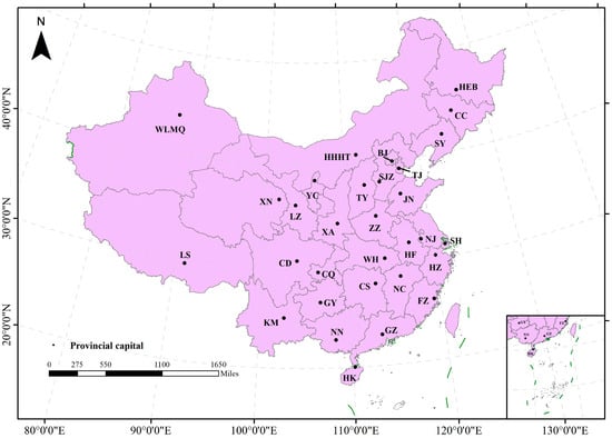
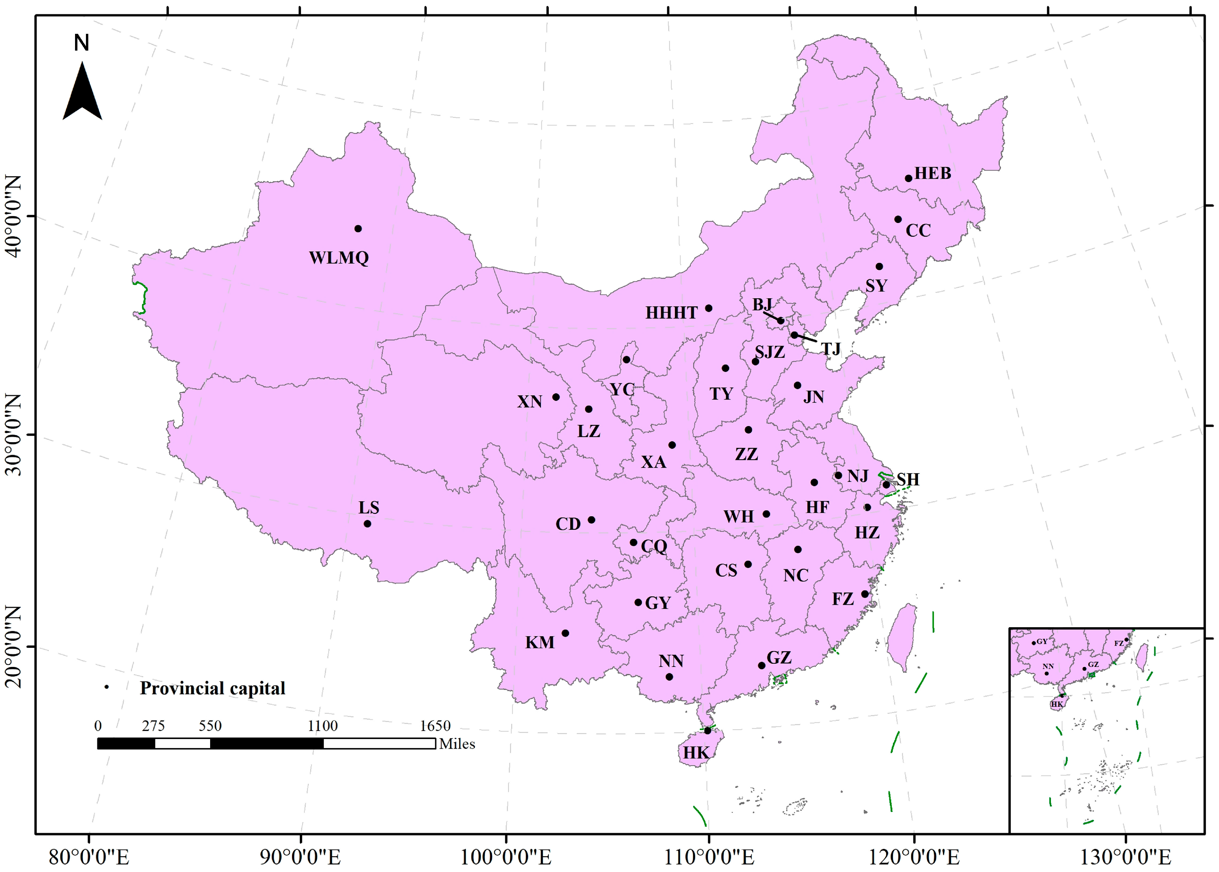
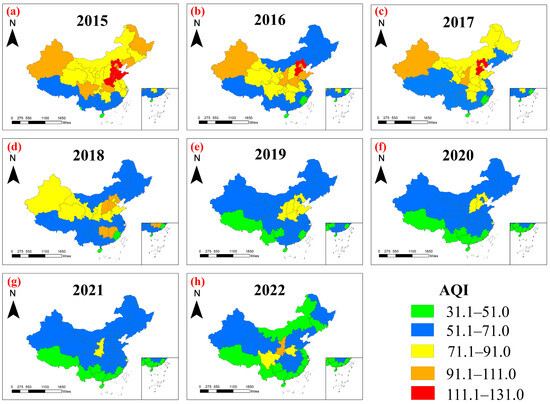
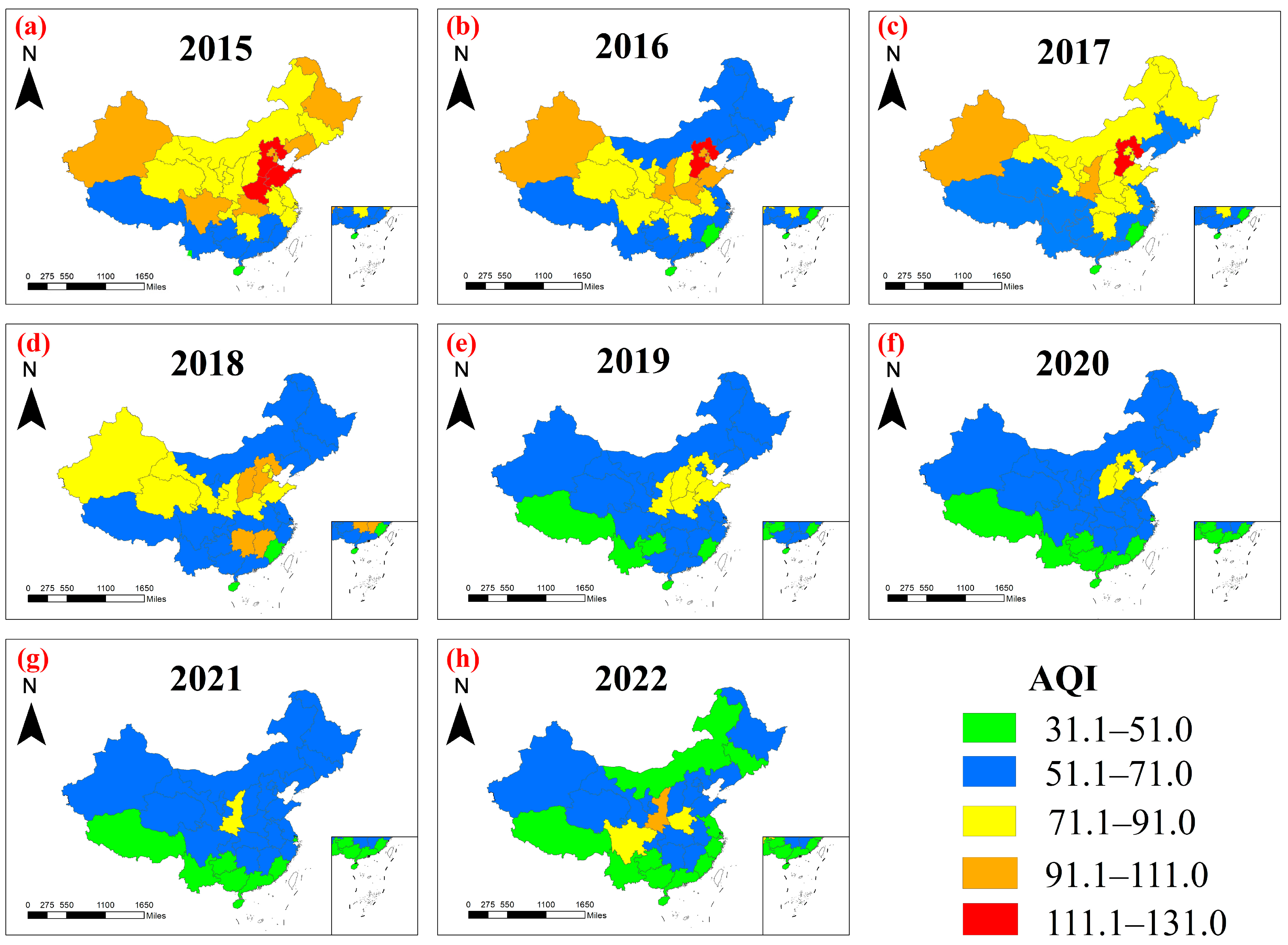
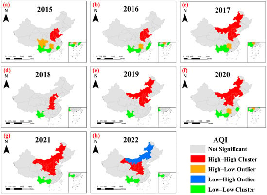
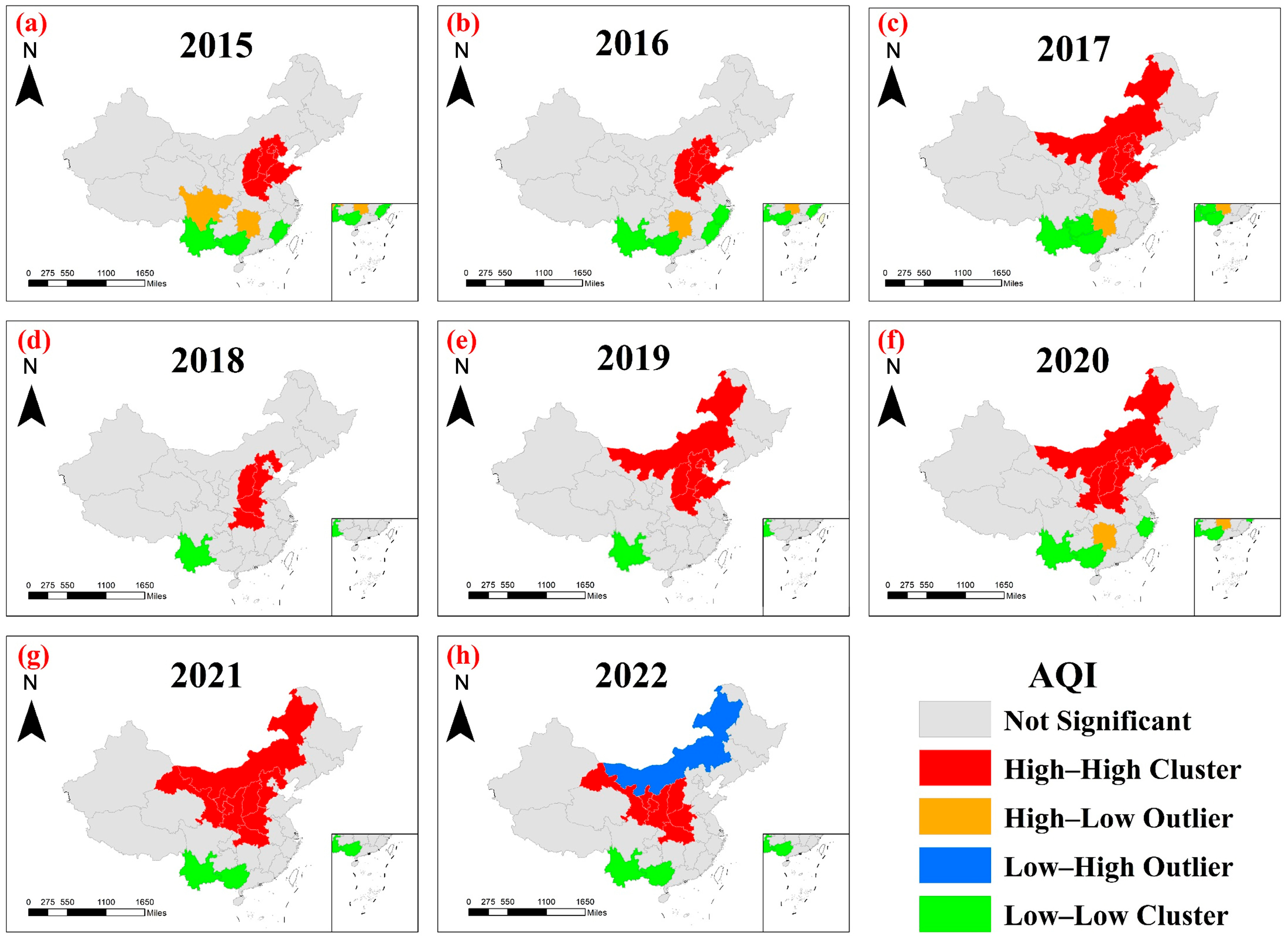
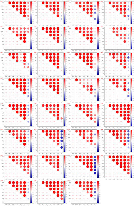
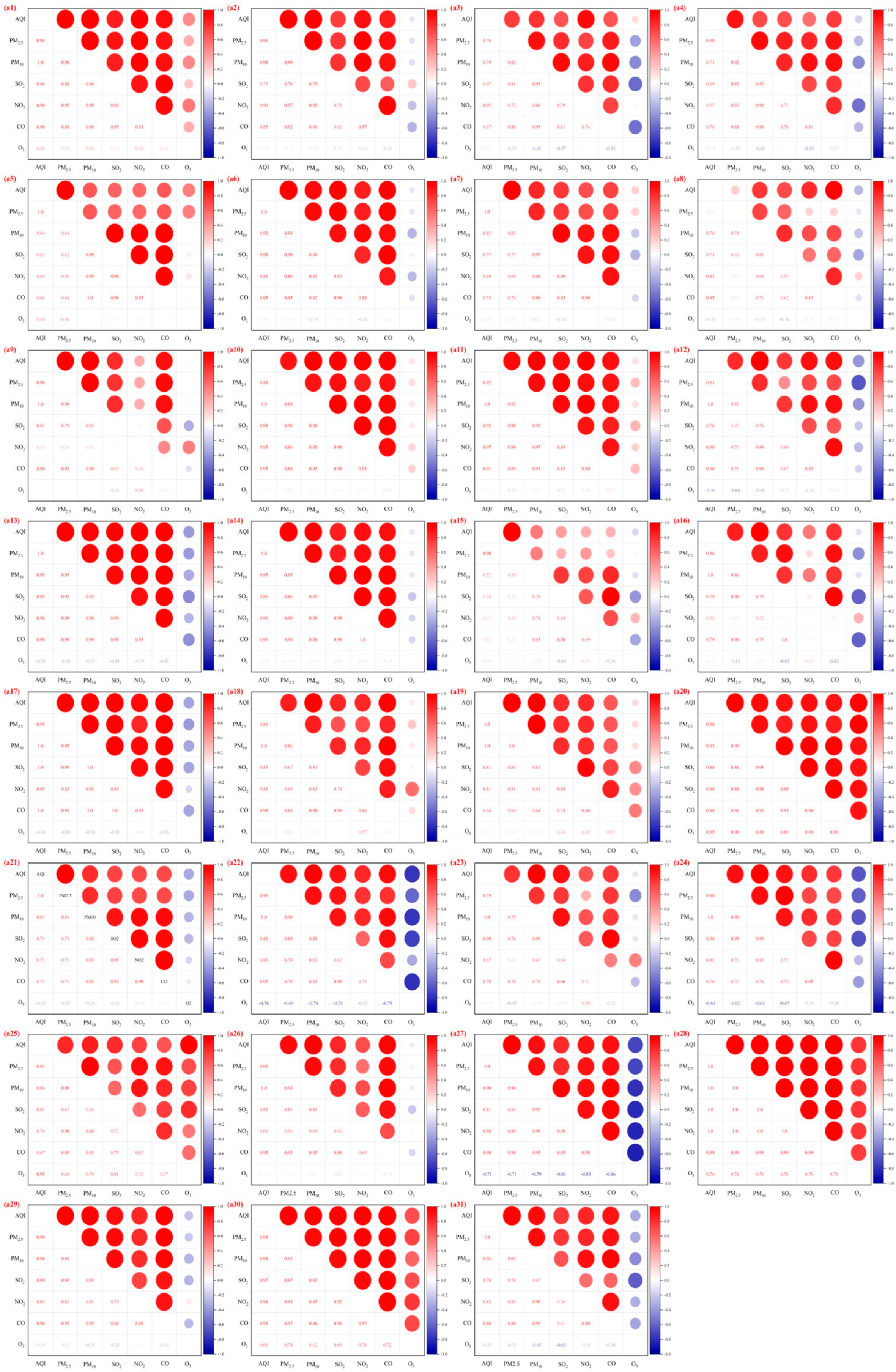
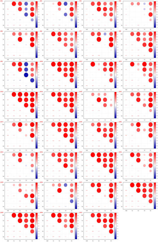
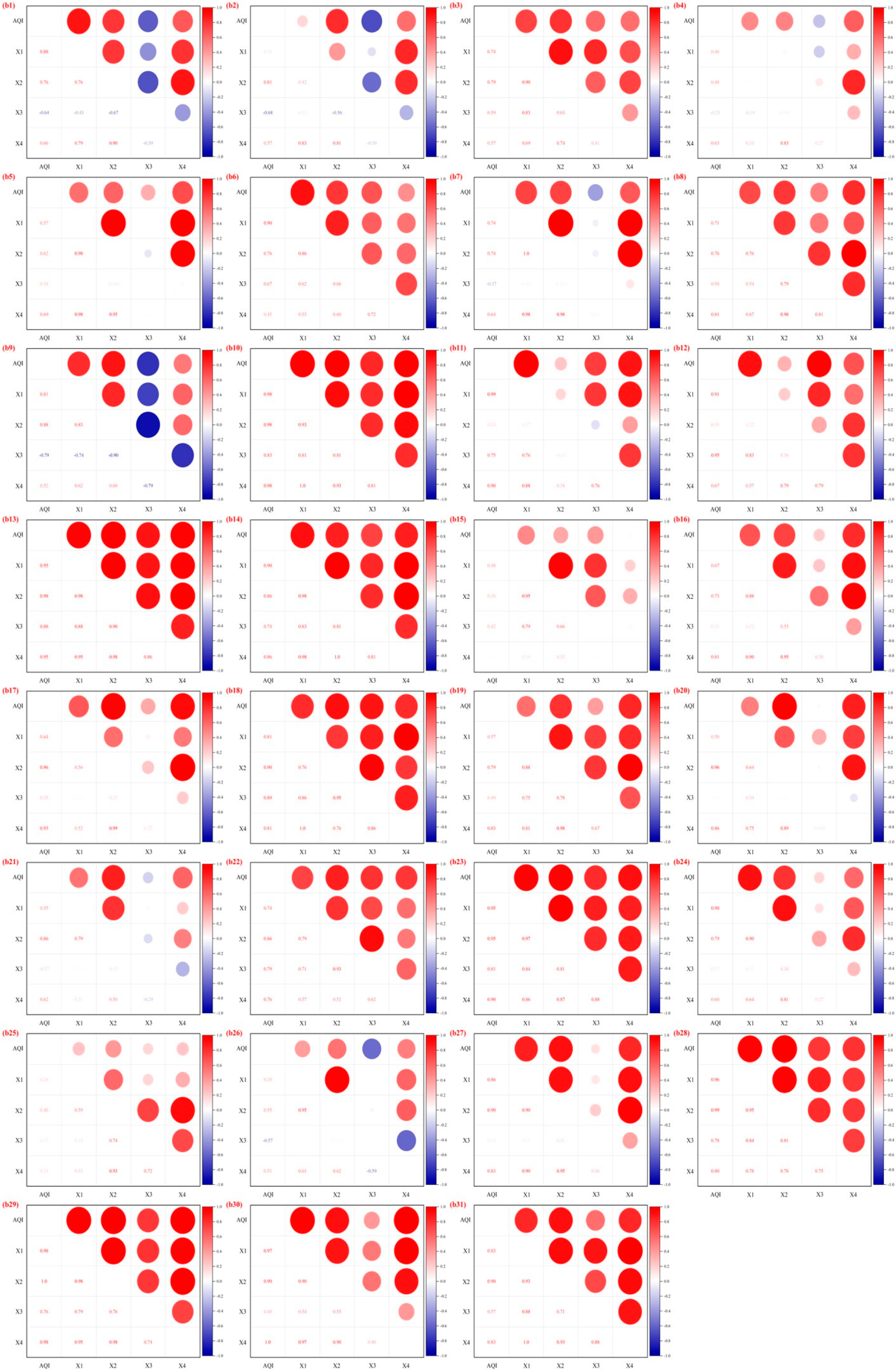
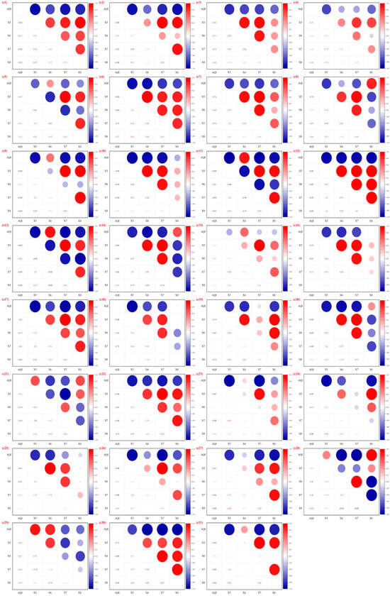
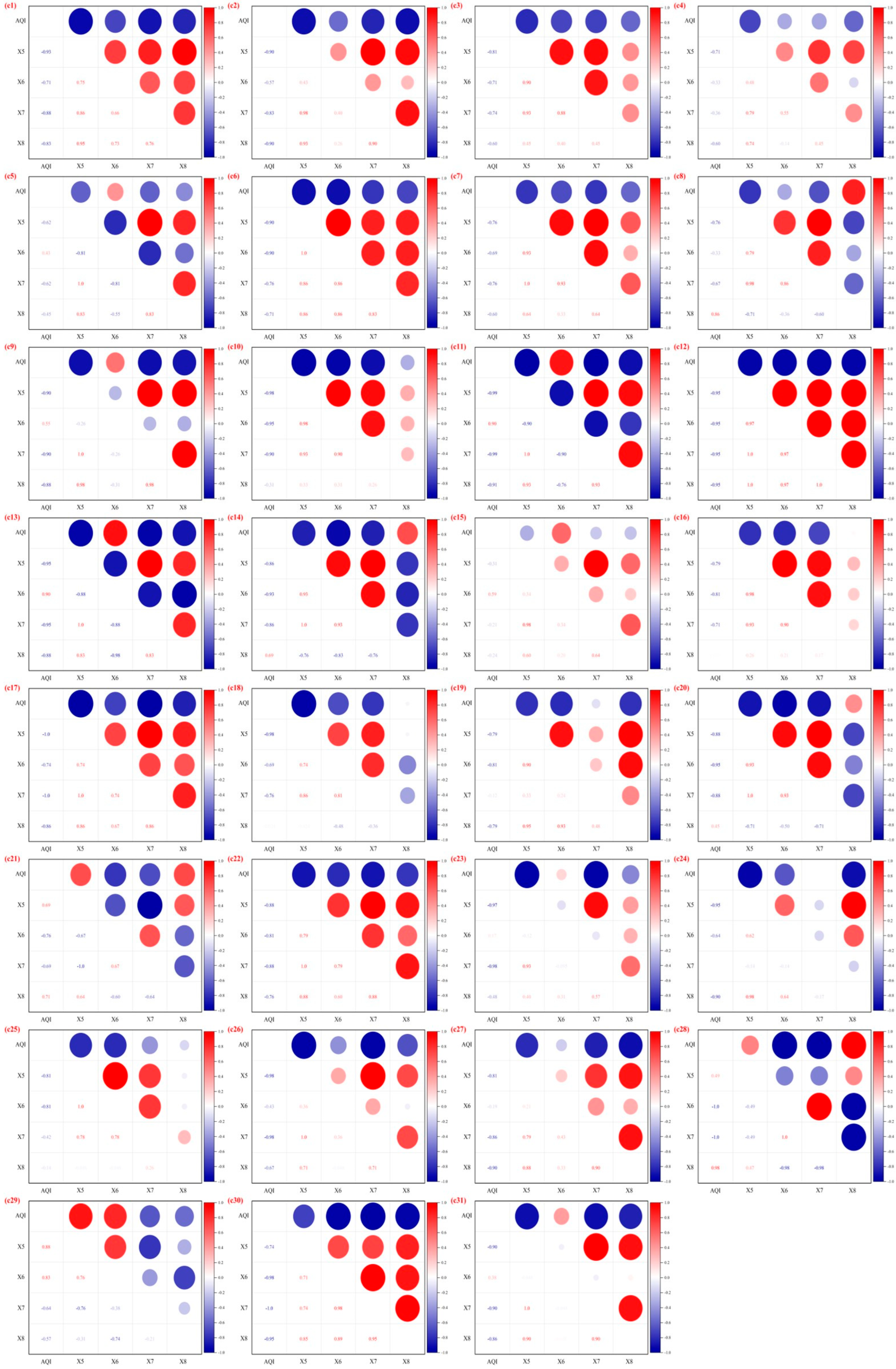
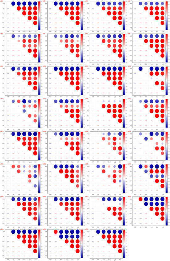
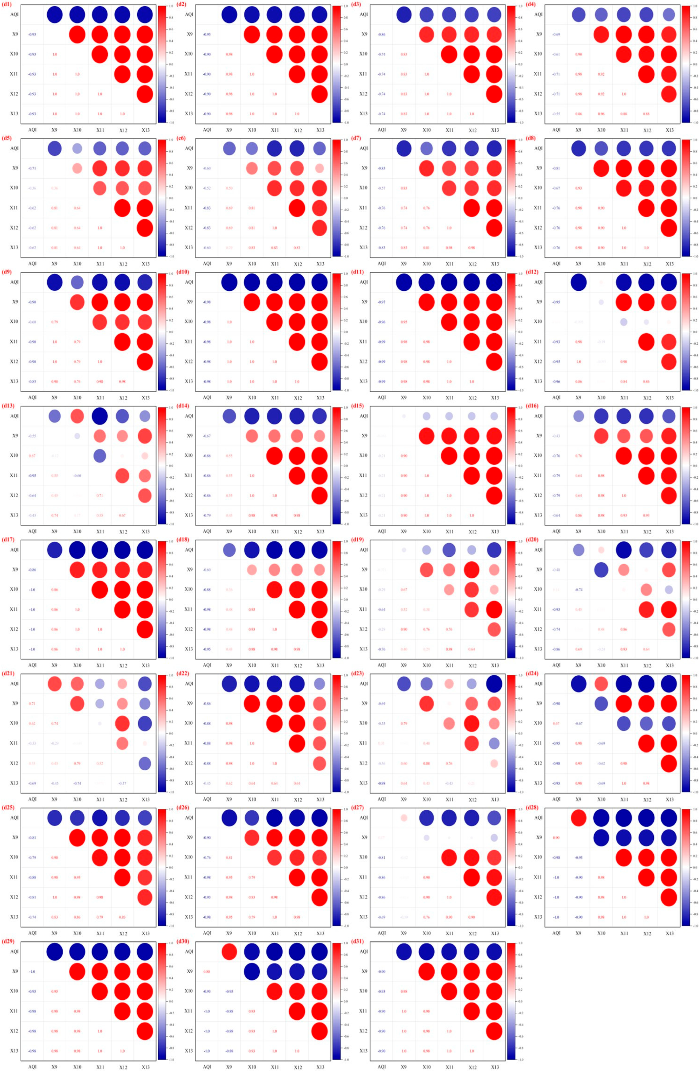
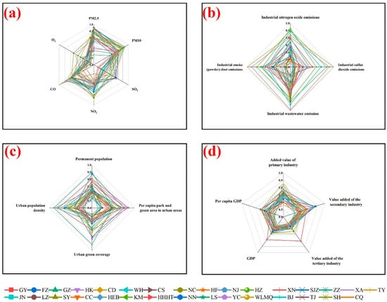
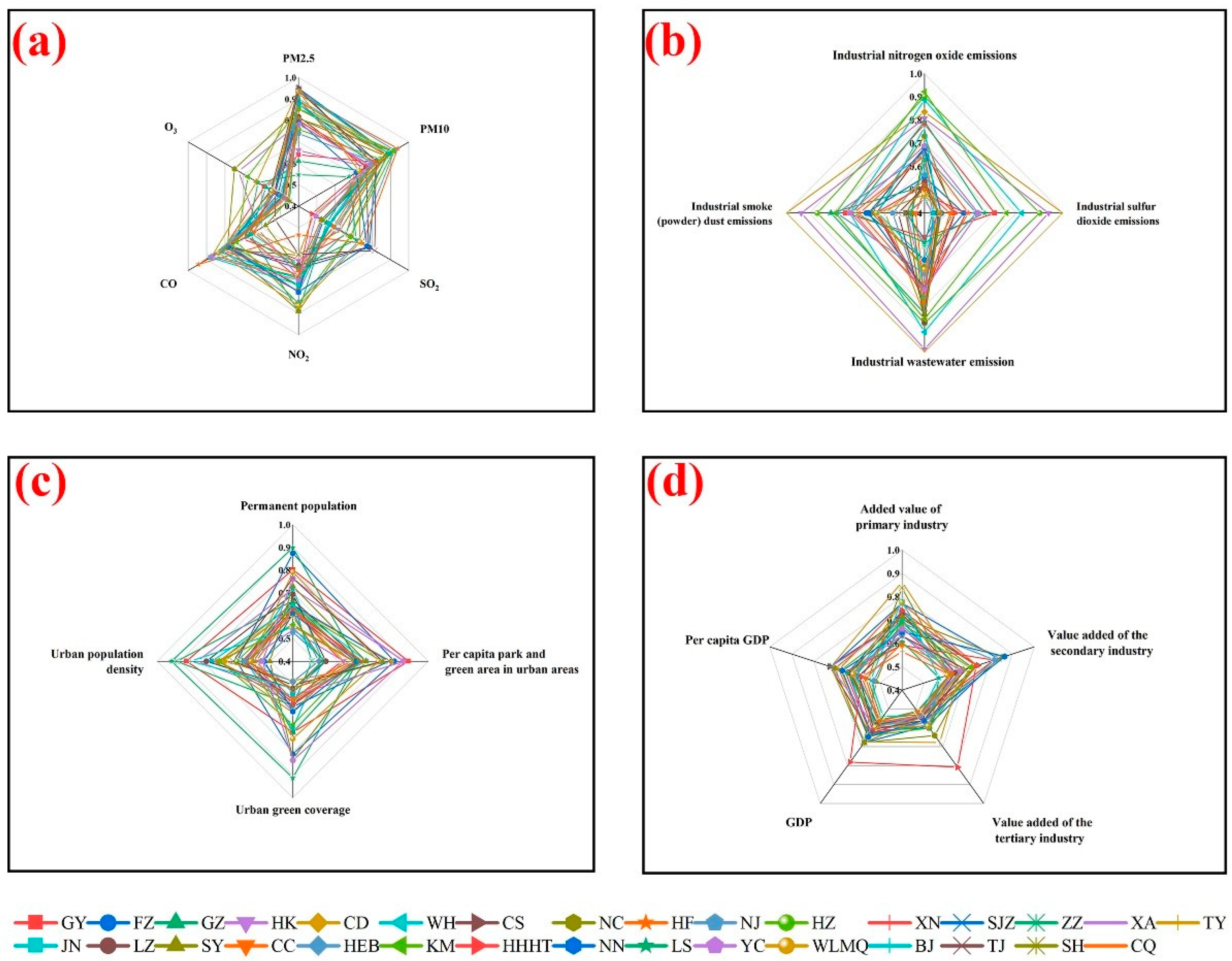
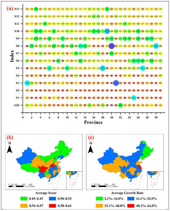
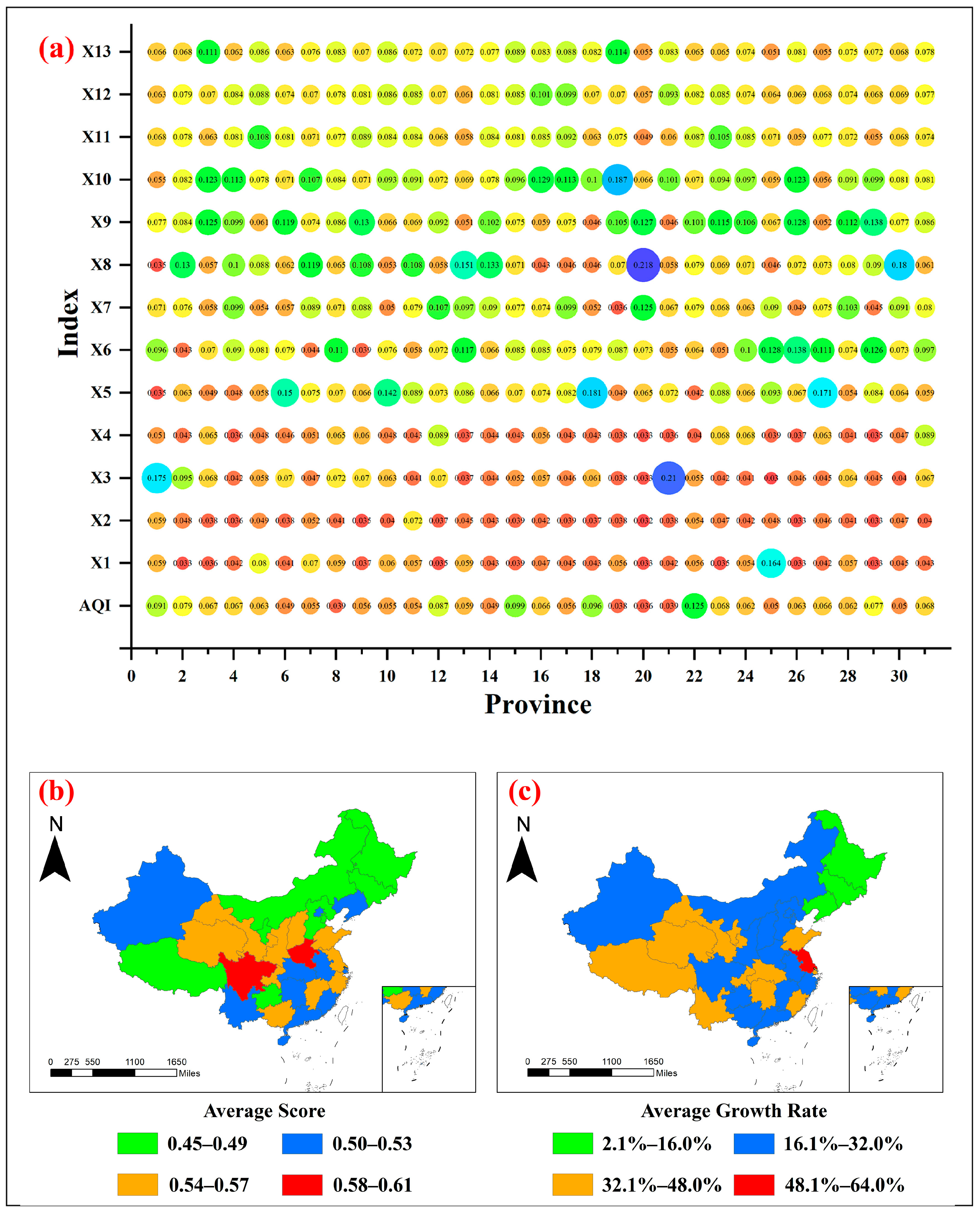
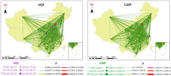
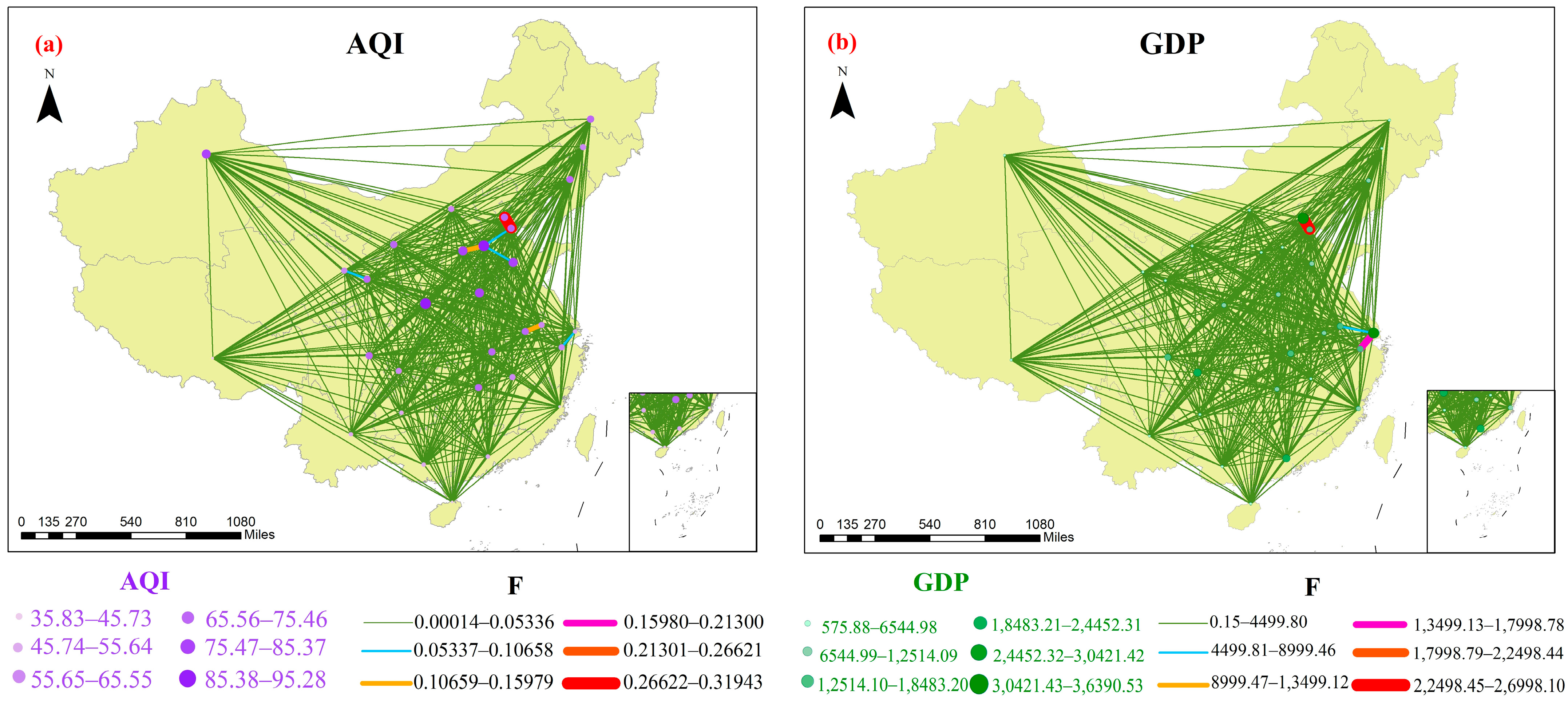
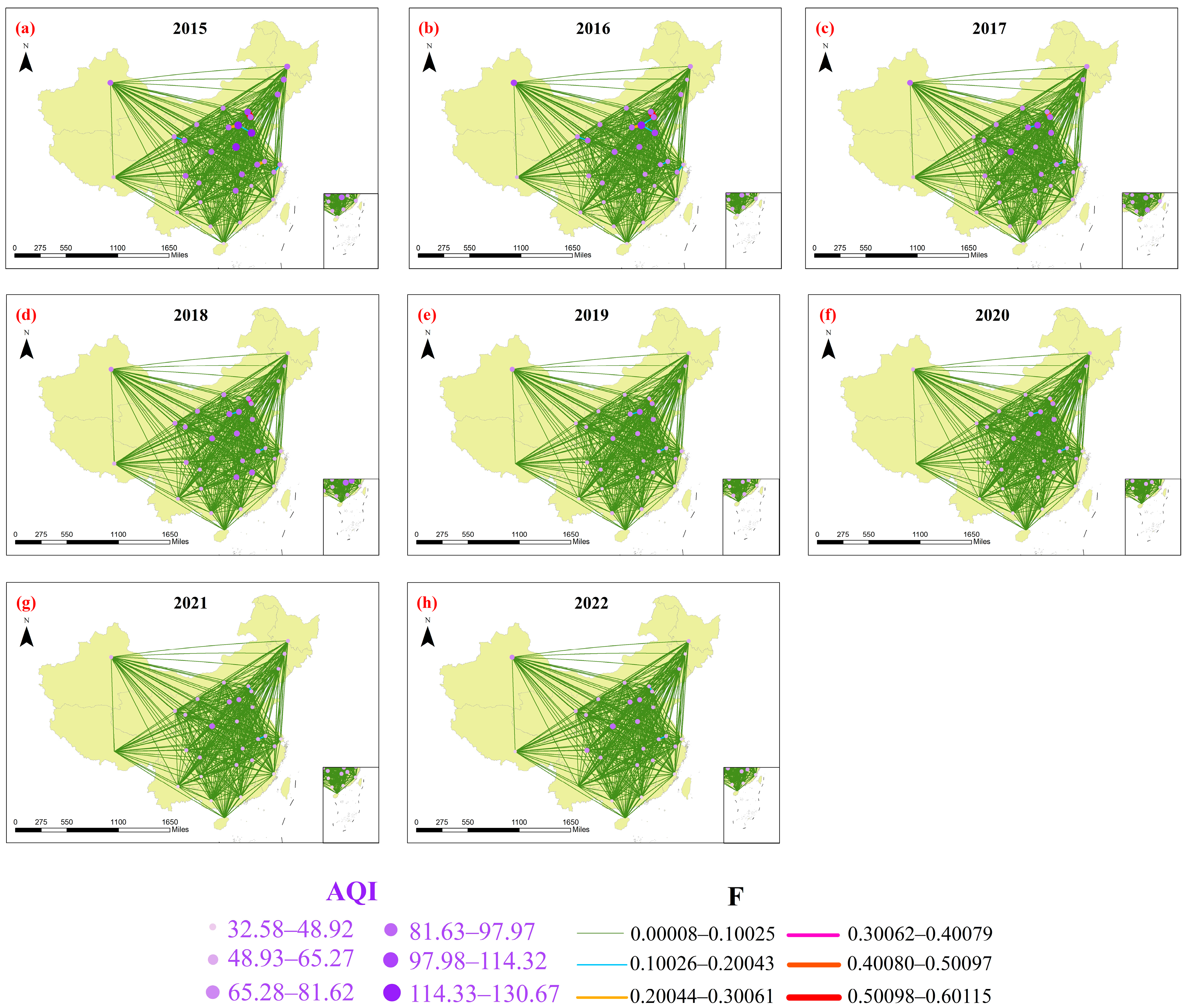
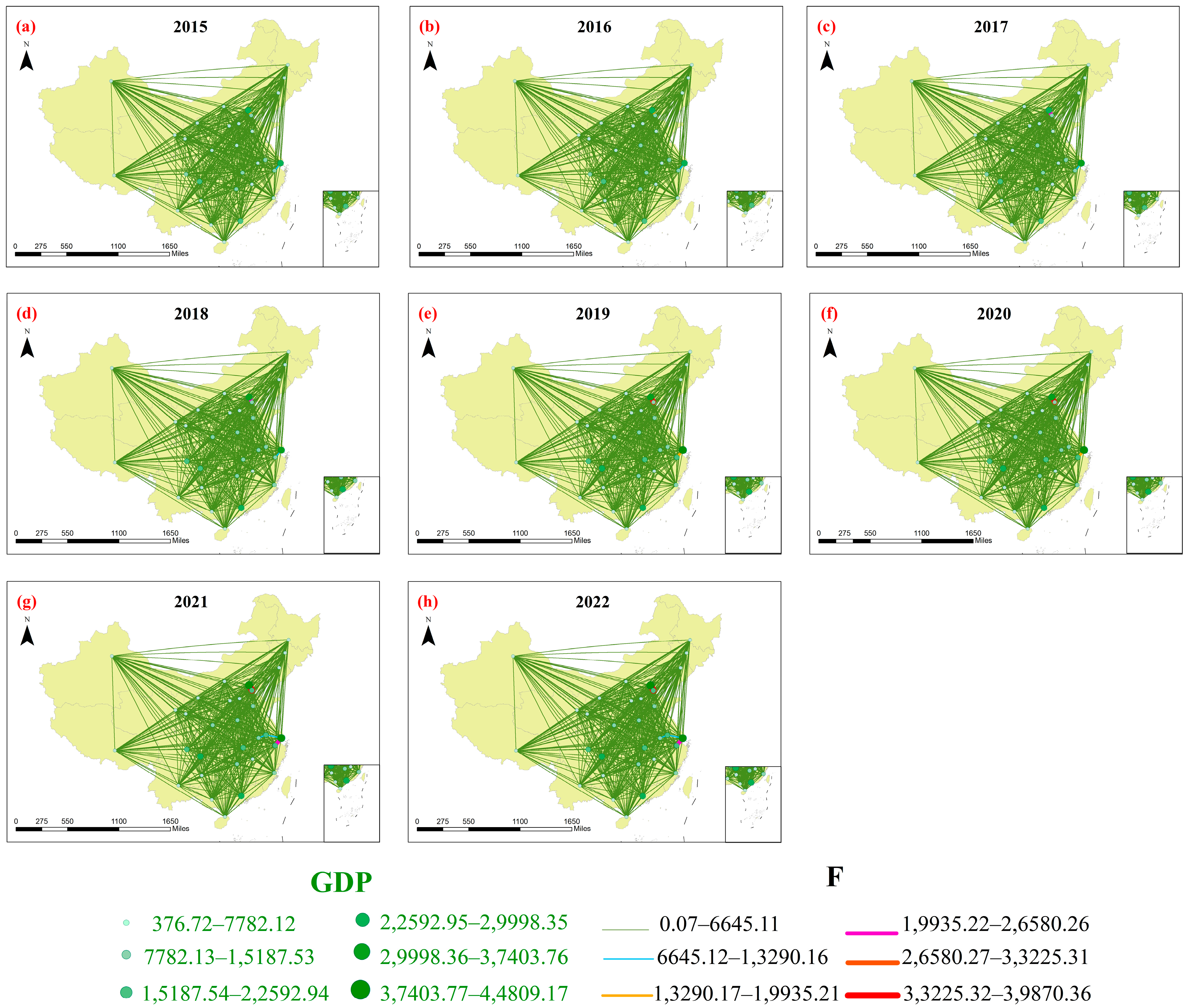

Disclaimer/Publisher’s Note: The statements, opinions and data contained in all publications are solely those of the individual author(s) and contributor(s) and not of MDPI and/or the editor(s). MDPI and/or the editor(s) disclaim responsibility for any injury to people or property resulting from any ideas, methods, instructions or products referred to in the content. |
© 2026 by the authors. Licensee MDPI, Basel, Switzerland. This article is an open access article distributed under the terms and conditions of the Creative Commons Attribution (CC BY) license.