


Abstract
Sustainable groundwater management in hyper-arid regions requires accurate water quality assessments, yet remote desert environments present major challenges due to data scarcity, high sampling costs, and limited laboratory infrastructure. This study proposes a framework integrating the Water Quality Index (WQI) with Inverse Distance Weighting (IDW)-based spatial data augmentation and machine learning classification for groundwater quality assessment in the Tabelbala region, southwestern Algeria. Three classifiers were evaluated, Random Forest (RF), Support Vector Machines (SVMs), and Artificial Neural Networks (ANNs), and trained on an augmented dataset generated from 178 original groundwater samples using IDW interpolation with a sensitivity-optimized 150 m radius, producing 2779 augmented training points. RF achieved the highest predictive accuracy (85.9%), followed by ANNs (84.7%) and SVMs (83.1%), with all models demonstrating excellent discriminative performances (area under the receiver operating characteristic curve > 0.96). Permutation Feature Importance analysis identified total dissolved solids (TDS), sulfates (SO42−), total hardness (TH), and chlorides (Cl−) as the most influential parameters, consistent with World Health Organization (WHO) guidelines. Spatial distribution maps revealed that the majority of groundwater sources exhibited poor to very poor quality, highlighting the urgent need for local water management interventions. The proposed framework offers a replicable decision-support tool for water resource managers in data-scarce arid environments, supporting SDG 6 (Clean Water and Sanitation) and SDG 13 (Climate Action).
1. Introduction
Water is an indispensable resource used for essential practices, such as drinking, agriculture, and industrial processes [1]. Among the various sources of water supply, groundwater resources play an important role in the development of human societies, providing nearly 50% of global drinking water and accounting for more than 40% of the water used for irrigation worldwide [1]. However, this essential reserve is under continuous threat owing to contamination and a progressive decline in overall quality [2]. This pressure arises from excessive human exploitation and the presence of various pollutants from industrial, agricultural, or domestic sources, which affect the health of the underground environment and cause irreversible damage [3]. This is especially true in rural regions, where the concept of vulnerability is closely linked to groundwater pollution, underscoring the importance of mitigating and controlling water pollution [4]. In this study, the rural area of Tabelbala, situated in southwest Algeria, was selected. Over the last decade, the region has suffered multiple human and environmental consequences, yet has remained habitable owing to its groundwater supplies [5]. These are considered essential for maintaining desert ecological processes, but most importantly, they constitute a vital water resource that satisfies the basic daily needs of the inhabitants of Tabelbala [5]. Consequently, the creation of a durable policy for water resource management, grounded in effective quality assessment measures, is critical. The main objective was to obtain quantitative information on the physical, chemical, and biological attributes of water sources [6]. Many water quality indices have been developed based on different concepts and knowledge about water issues [7]. The most popular assessment measures [8] include the National Sanitation Foundation Water Quality Index (NSFWQI), the Canadian Council of Ministers of Environment Water Quality Index (CCMEWQI), the British Water Quality Index (BWQI), the Environmental Performance Water Quality Index (EPIWQI), and, our chosen index, the Water Quality Index (WQI) based on World Health Organization (WHO) standards [8]. In the literature, various authors have described the “WQI” for groundwater to illustrate annual cycles, spatiotemporal variations, and trends in water quality [9]. The index, often noted as GWQI or WQI, is a universal measure that is considered to be the most efficient and robust in this case, compared to other indices that are more localized metrics, showing the best performances in the regions where they were developed [7]. In addition, a large part of Algeria is covered by arid and semi-arid regions [10], including our area of study, Tabelbala, where, as previously cited, limited access to surface water resources has historically forced populations to rely heavily on underground aquifers to meet their water needs [5]. To generate a clear picture of groundwater resource quality under such climates, many researchers worldwide have used the WQI model. In the study of de León et al. [11], the authors analyzed the effects of drought and groundwater quality, as measured by the WQI, on agricultural production and domestic use. Ahmad et al. [12] used the WQI for an accurate water quality assessment in the Emirate of Abu Dhabi, UAE, which is classified as a hyper-arid climate and faces water scarcity challenges. Similarly, Algerian researchers have relied heavily on the WQI model to assess the quality of groundwater resources. In the paper by Houari, Bouselsal and Lakhdari [10], a study was conducted using the WQI to evaluate the suitability of water for domestic consumption in the presence of high nitrate levels. The article by Hamlat and Guidoum [13] assessed the status and trends in groundwater quality of 12 aquifers in northwestern Algeria under drought conditions using the WQI over a 4-year period. All studies reported accurate results when integrating the WQI model. Although the WQI can be computed directly from measured parameters using a deterministic formula, practical monitoring programs often face incomplete measurements or delayed laboratory analyses [14,15]. In such situations, machine learning models can provide rapid predictions of WQI classes based on available hydrochemical variables. Recent studies have demonstrated the ability of artificial intelligence models to capture complex nonlinear relationships between input parameters and target variables, often achieving a better predictive performance than conventional regression approaches [16].
In this study, three models, namely, Random Forest [17], Support Vector Machines [18], and Artificial Neural Networks [19], were selected and trained using open-source platforms, achieving state-of-the-art results. These models were chosen based on their ability to handle the features of a water quality dataset and their efficiency in similar situations [20]. They constitute powerful algorithms capable of learning patterns and relationships across multiple datasets for the accurate and efficient prediction of WQI classes [21,22]. For example, Wang et al. [23] used four machine learning algorithms, including Support Vector Machines (SVMs) and Random Forest (RF), to establish an effective and reliable WQI model for assessing coastal water quality in Cork Harbour, Ireland. The results indicated that the various predictive models achieved outstanding performances with accuracies above 99%. Moreover, Wang, Zhang and Ding [23] demonstrated that integrating machine learning algorithms, such as Artificial Neural Networks (ANNs), WQI, and remote sensing spectral indices, afforded an efficient model for water quality assessment. In addition, these classifiers have the significant advantage of being less sensitive to multicollinearity, which can affect the accuracy of predictive models for water quality assessment, thereby favoring their use [24]. Another issue to consider when dealing with water quality data is the limited number of available samples, which can limit the performance of machine learning models [25]. To address this problem, interpolation techniques are often used to increase the sample size [25]. This is the case for our proposed methodology, which integrates an Inverse Distance Weighting (IDW) technique to overcome the lack of viable samples [26]. Spatial interpolation techniques, such as IDW, are widely used to estimate unknown values from nearby observations and have demonstrated strong performances in environmental and geotechnical mapping when spatial heterogeneity is present [27]. The generated inputs were used with the selected classifiers to increase their accuracies to over 80%. Model performance was further assessed using precision, recall, and the F1-score, which are widely used evaluation metrics that measure the reliability of positive predictions, the ability to detect relevant instances, and the balance between these two aspects [28]. Finally, receiver operating characteristic (ROC) curves were generated for all models to further validate the proposed method [29]. Ultimately, the proposed work is the first to combine the Water Quality Index (WQI), data augmentation techniques (IDW), and machine learning classification models within the Tabelbala region, aiming to produce an accurate and time-effective water quality assessment method utilizing open-source platforms.
2. Materials and Methods
2.1. Study Area
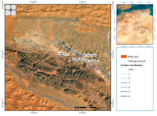
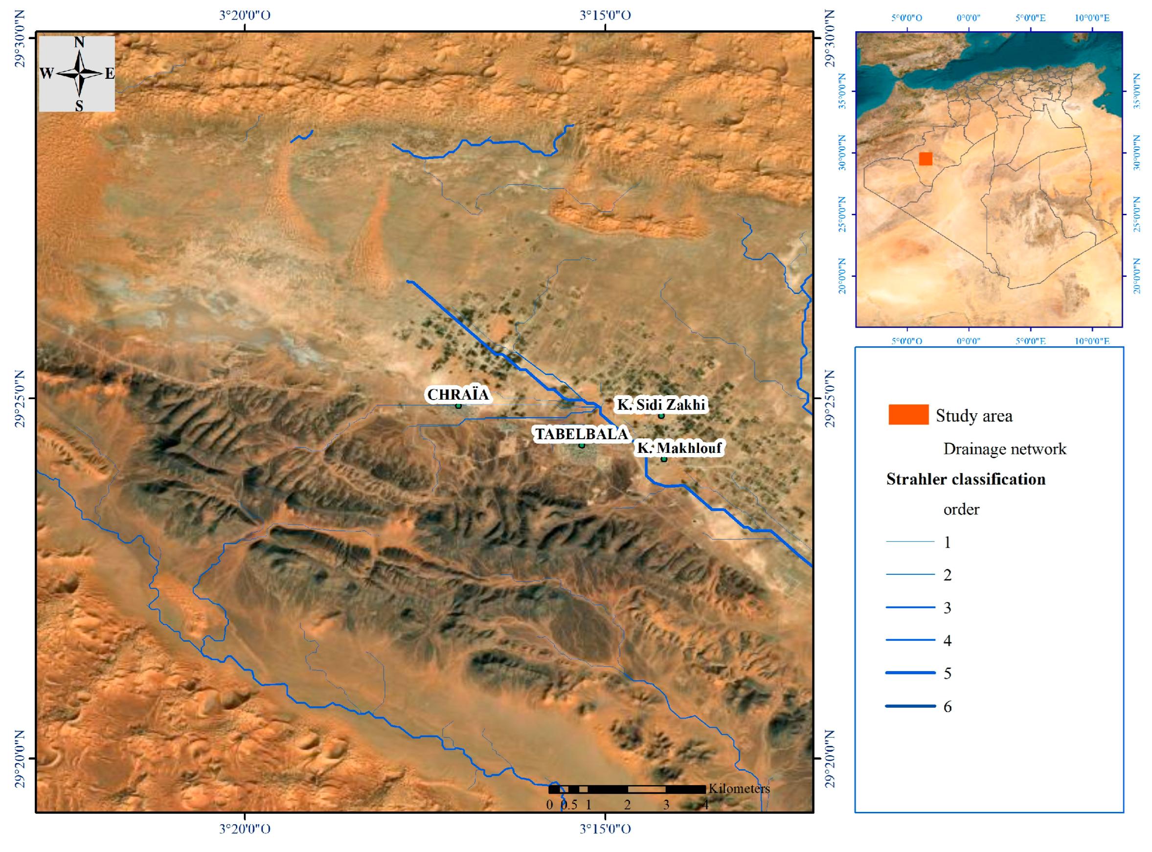
Tabelbala is an Algerian city affiliated to the wilaya of Beni Abbes, located approximately 400 km south of Bechar, at geographic coordinates 29°24′22″ N and 3°15′33″ W (Figure 1). The region forms part of the relief system known as the “Ougarta Mountains” and is especially famous for its Acheulean industries [30]. It covers an area of approximately 60,560 km2, with an average elevation of approximately 522 m, and a total of 5448 inhabitants in 2008 [30], according to the estimates provided by the Department of Planning and Land Management (DPAT). The population has recorded a significant annual growth rate of 1.44% and is expected to reach 6656 inhabitants by 2024 [5]. This growth results in an increasing demand for drinking water, which is approximately from 493 to 588 m3 per year. The considered region exhibits a desert continental climate, with an average annual precipitation of less than 50 mm/year, according to NASA POWER data for the period 1981 to 2021 [31]. During the same period, the mean annual temperature in this area was estimated to be approximately 25 °C.
Figure 1.
Study area location.
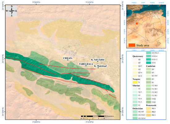
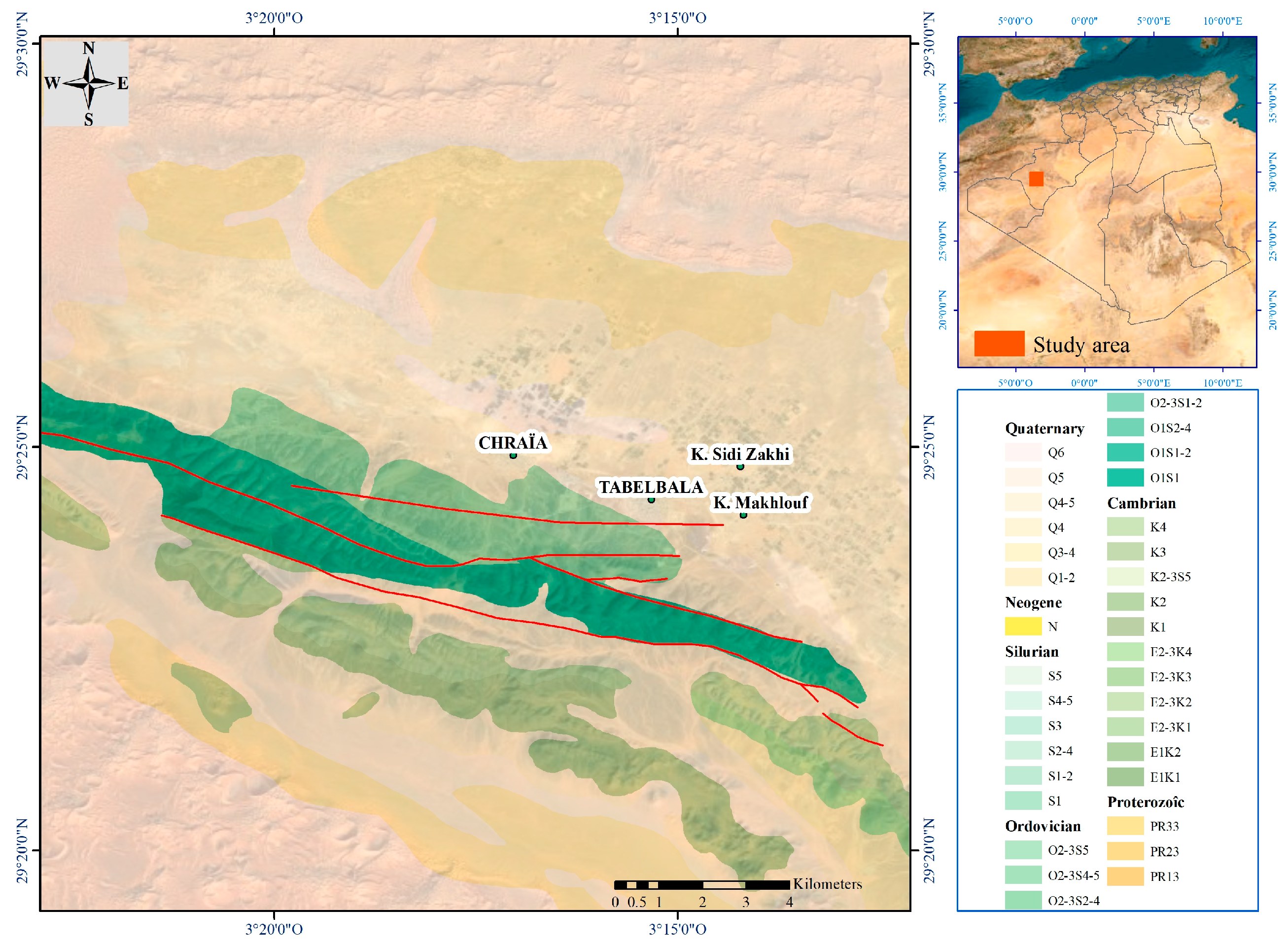
In the region of Tabelbala, the drainage network is well organized following the northwest–southeast-oriented geological structures. Oued Daoura is considered as the primary watercourse in the city [5]. The study area is part of a basin that hosts multiple aquifer formations distributed across various stratigraphic levels, ranging from the Cambro-Ordovician to the Quaternary. These aquifers are primarily distinguished by their lithology, thickness, and water quality (Figure 2). Several aquifers have been identified including the Cambro-Ordovician aquifer, the Hamada of Daoura aquifer, the Erg Er Raoui aquifer, and the Tabelbala aquifer. Each of them exhibits distinct characteristics in terms of composition and hydrogeological potential [32].
Figure 2.
Hydrogeological map of the study area.
The excessive pumping and exploitation of groundwater resources, in association with rarer rainfall, given Tabelbala’s climate, are significantly contributing to the dryness and degradation of their quality [33]. This study focuses on evaluating the quality of groundwater supplies in the city of Tabelbala, which are crucial to the area’s development and sustenance.
2.2. Water Quality Index (WQI)
The WQI is a universal mathematical measure used to assess groundwater bodies based on a set of significant physicochemical factors that typically reflect their health [7]. The index offers the advantage of combining all the complex information from the selected factors into a single value, making it easier for the general public, policymakers, and environmental scientists to understand the status of water resources. The index formula based on the standards established by the World Health Organization (WHO) [34] is given as follows:
where is the sub-index value for the factor calculated by using the relative weight and water quality rating Their formulas are defined as follows:
Here is the weight of the factor and it is assigned depending on its relative importance to the drinking water quality according to the World Health Organization (WHO) 2011 standard limits [34].
The water quality rating is a percentage ratio of a sample’s concentration in the factor and the drinking water standard limit of that same factor .
A lower WQI value usually indicates good water quality, while a higher GWQI value indicates poor water quality. The WQI classification rates and the corresponding water quality indicators as defined by the WHO [34] are given in Table 1.
Table 1.
WQI classification rates and quality indicators.
In this work, the calculated WQI values for our samples range between approximately 50 and 511, corresponding to four water quality classes: good, poor, very poor and unsustainable for consumption.
2.3. Data Collection
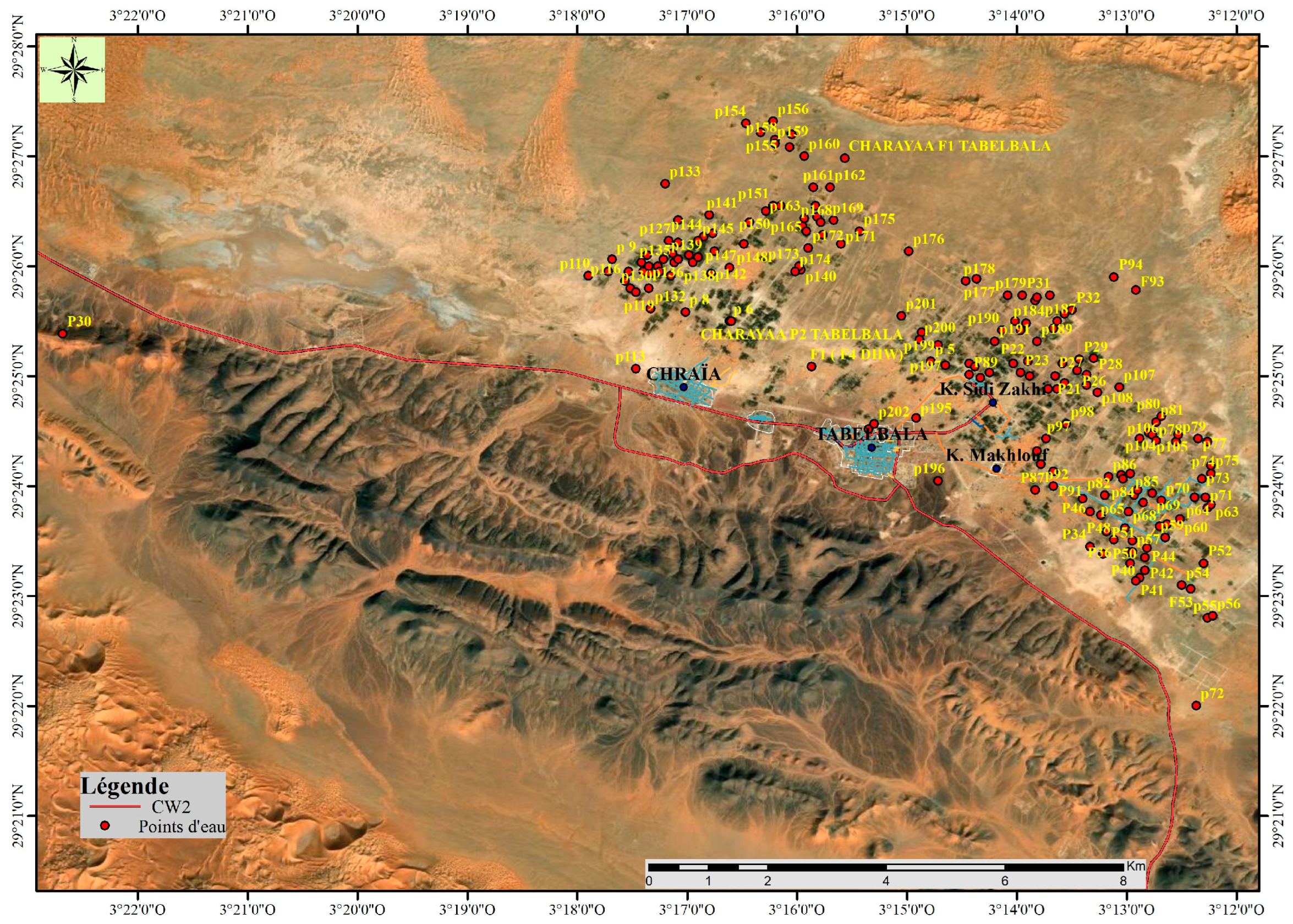
The experiments involve the collection of 178 water samples taken from multiple sites across Tabelbala during March 2024 (Figure 3). The selected instances, mostly wells and boreholes, were selected based on data availability and their significance for groundwater extraction and consumption. Each sample groups a series of physicochemical parameters or factors, including pH levels (pH), bicarbonates (HCO3−), chlorides (Cl−), nitrates (NO3−), sulfates (SO42−), sodium (Na+), potassium (K+), calcium (Ca2+), magnesium (Mg2+), total dissolved solids (TDS), and total hardness (TH). All concentration values were measured using standardized water testing procedures and equipment. In addition, the different locations of each sample were recorded through a global positioning system (GPS).
Figure 3.
Spatial distribution of boreholes in the study area.
Details of assigned weights of each parameter according to their relative importance in terms of drinking water quality and their standards limits , for groundwater assessment, are given in Table 2. These limits are selected as per the values recommended by the WHO in 2011 [34].
Table 2.
Unit weight of each of the physiochemical parameters used for WQI.
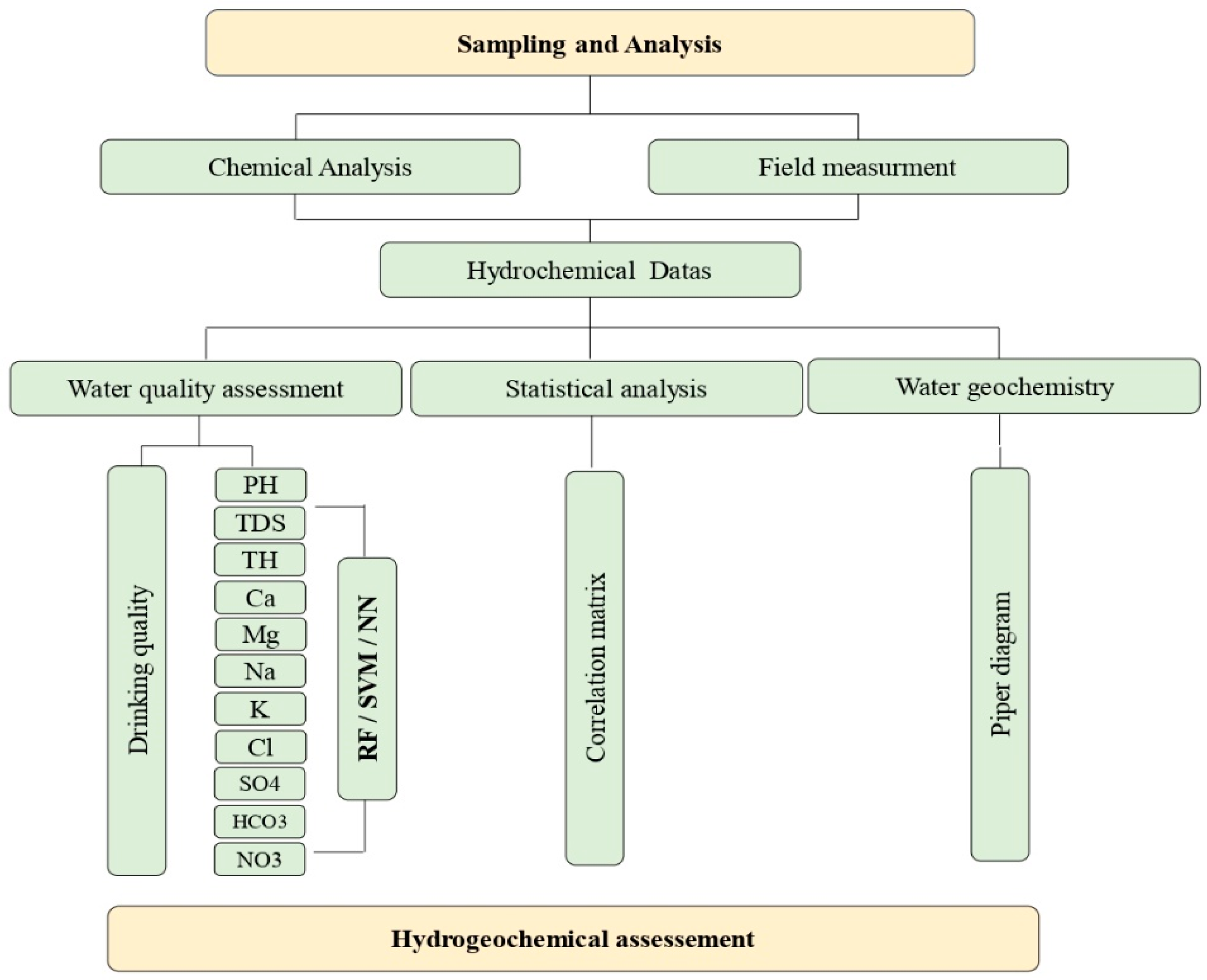
The maximum weight value of 5 is assigned to factors such as Cl−, NO3−, TDS and SO42− that are crucial in water quality evaluation. On the other hand, factors such as HCO3− are assigned a weight value of 1 and are considered less significant in this context. The methodology adopted is presented in Figure 4.
Figure 4.
Flow chart of the adopted methodology.
2.4. Data Augmentation Using Ordinary Inverse Distance Weighting
Typically, field campaigns are tedious, time-consuming, and often expensive to implement, making it impossible to collect enough inputs to produce high-precision results for machine learning models [35]. In practice, it is common to perform a mathematical operation called data augmentation to increase the number of samples. Many techniques exist, including Inverse Distance Weighting interpolation, which assigns weights to nearby measurements to calculate a weighted average, with closer observations exerting greater influence [36]. The goal is to estimate unknown values at specific points using known samples from surrounding locations. The IDW is the simplest type of interpolation and is often used to augment water quality data [37,38,39]. It offers the advantage of being fast and easy to implement, providing good computational efficiency, and the method works well with small datasets. Contrary to advanced interpolation techniques, such as the well-known ordinary kriging [40], which fits complex variograms to the data based on numerous neighboring samples, IDW can generate a new data point using only two observations.
In this study, an IDW-based interpolation was conducted in a 150 m radius surrounding each sample to increase the number of inputs. The use of a limited area (150 m) is essential to achieve better reliability [41]. Given that IDW encounters difficulties when extrapolating to locations distant from existing measurements and that water quality may shift drastically from one location to another, maintaining a relatively small radius is a reasonable assumption for achieving accurate results. Each water attribute was separately augmented and then combined with other factors to produce final samples. The selection of the 150 m interpolation radius was guided by sensitivity testing and the spatial representativeness of the augmented dataset. Several candidate distances (60 m, 90 m, 120 m, and 150 m) were evaluated to analyze their influence on the number of generated samples and the predictive performance of the selected ML models. The results indicated that increasing the interpolation radius generally reduced the root mean square error (RMSE) of the predictions. Among the tested configurations, the 150 m radius produced the lowest RMSE while maintaining local hydrochemical variability. Therefore, this value was selected as a reasonable compromise between generating a sufficient number of augmented observations and preserving the spatial consistency of groundwater quality patterns. The number of augmented training points for each radius value and the corresponding RMSE values for each model are listed in Table 3. Both metrics were averaged across several cross-validation folds (see the next Section 2.5 Data Splitting) to provide a representative estimate of model performance. As shown, increasing the interpolation radius increases the number of augmented points and generally reduces RMSE for all classifiers, with a radius of 150 m yielding the lowest errors.
Table 3.
Number of augmented points using different radius values.
The name IDW refers to the fact that the method assigns weights that are inversely proportional to the power of the distance between the locations of the generated points and the known measurements. The method formula is given as follows:
Here is the interpolated value at new point , and is the value of known sample . The weight () that is given to each point can be calculated as follows:
Here is the distance between the interpolated point and the original point, and is the power variable that affects the weight of nearby samples. During our experimentation, the IDW parameters are set to a maximum of 5 neighbors and a power variable of to maintain good data reliability. Similar to defining a relatively small radius for interpolation, limiting the number of neighbors per pixel for IDW calculation and setting the parameter to 2 help avoid over-smoothing of the data while maintaining good local variability. In addition, the original water instances were added to the augmented observations to preserve their attribute values and increase classification performance.
2.5. Data Splitting
Before applying the IDW augmentation technique, the original samples were partitioned into training and test sets using K-fold cross-validation (CV) [42]. During the CV process, all instances are randomly split into K parts; the model is trained on K − 1 parts, with one fold held out for testing, ensuring each segment is used for both training and testing [43].
This cross-validation procedure often yields a high performance and does not waste much data, as only one group is removed from the training set. Selected models are trained on each fold separately. The results are finally averaged to ensure the built model learns from the entire dataset.
In practice, it is often found that splitting is performed after data augmentation. Despite its high performance, the use of such a process may have introduced bias due to data leakage [44]. Data interpolation methodologies, by nature, often generate highly correlated samples. Therefore, to preserve independence between the training and test sets and avoid dependent model evaluation, the data were partitioned first. IDW is next used to increase the number of training observations to an adequate level. However, the lack of initial samples inevitably led to fewer testing instances. As shown in Table 4, each testing fold contains between 32 and 37 original samples, representing approximately 20% of the 178 total observations. Therefore, the reported performance metrics should be interpreted with caution; this limited test set size may not fully reflect the model’s generalization ability to unseen regions or datasets with different hydrogeological characteristics. Spatial intersections between training and testing datasets were verified for each fold to ensure that no augmented samples overlapped with testing locations, thereby reducing the risk of interpolation-based data leakage. However, since folds were generated randomly, some spatial proximity between samples may still exist. Spatial cross-validation strategies (e.g., block-based or distance-based splitting) were considered but could not be implemented given the dataset constraints. With 178 original samples and K = 5 folds, each training split already contains approximately 143 observations, and each testing fold between 32 and 37 instances (Table 4). Further spatial partitioning would produce training blocks of fewer than 100 samples, insufficient for reliable four-class model training. This constitutes a recognized limitation of the current study, and spatial cross-validation is recommended for future work when a larger dataset becomes available. It should be noted that no formal spatial autocorrelation test was applied to the residuals, which constitutes a recognized limitation of the current study. While the implemented precautions, pre-split augmentation, training-only IDW application, and overlap verification, reduce spatial dependence, they do not fully eliminate it.
Table 4.
Number of training and testing samples for each split fold.
The IDW augmentation was performed post splitting with K = 5 folds using the Scikit-learn Python 3.11 library, in combination with the three classifiers: Random Forest, Support Vector Machines, and Artificial Neural Networks (Multi-Layer Perceptron). The number of augmented training samples (including original observations) and corresponding testing instances for each fold are reported in Table 4.
The IDW-based augmentation procedure, applied to increase the training set from 178 to over 2000 samples, produced highly correlated synthetic observations derived from the original measurements. These augmented points did not introduce independent variability but helped improve model stability during training. Importantly, the testing set consisted only of original samples, ensuring that the evaluation remained independent.
2.6. Machine Learning Models
The proposed methodology aims to develop a machine learning model for water quality assessment based on a dataset with 11 features (physicochemical factors). All instances were preprocessed, including data normalization and balancing for the training samples, whereas the test sets were normalized only. Data balancing techniques include under-sampling of majority classes and over-sampling of minority classes. For data normalization, mean and variance scaling is applied to avoid the impact of features on each other while improving ML training and avoiding extra biases. Although, such a process is unnecessary in the case of RF, as the absolute scale of the features does not matter in this case.
A model’s performance and highest accuracy depend on its best parameters, called hyperparameters [45,46]. Several techniques have been proposed for tuning the optimal parameters during the training phase, such as the grid search procedure [43,47]. Hyperparameter tuning was performed using only the training data. Several candidate values were tested for each algorithm, and the optimal combination that achieved the highest average cross-validation accuracy across all folds was determined using the grid search procedure. Different parameters were selected for each model because of their significant influence on the results; they were optimized using the grid search technique exclusively on the training data. The search ranges and best values for each classifier are summarized in Table 5, Table 6 and Table 7, respectively.
2.6.1. Random Forest
Random Forest is a popular machine learning algorithm that constructs a tree-like structure to combine multiple outputs into a single decision. The efficiency of RF is mainly due to its ability to handle complex datasets and mitigate overfitting [17]. Each tree determines a partial solution of the problem using either a bagging principle, which consists of training several weak models on different subsets of the data [48]. Finally, the combination of uncorrelated trees lowers the overall variance, multicollinearity risk, and prediction error. The RF classifier is typically utilized as a bagging algorithm for water quality assessment [49,50]. In the case of RF, four parameters were optimized using the grid search technique; their best obtained values are presented in Table 5.
Table 5.
RF grid search parameters, ranges and best values.
The hyperparameter ranges were selected to explore both simple and complex model configurations while preventing excessive model complexity that could lead to overfitting.
2.6.2. Support Vector Machines
Support Vector Machines (SVMs) are commonly used in water quality assessment problems [48,51]. They distinguish between Water Quality Index (WQI) classes by finding the hyperplane with the largest margin that maximizes the separation between the classes in the training data. These types of algorithms are particularly useful when dealing with multiple features. In addition, a combination of kernel techniques and SVMs enables the distinction of nonlinear patterns and relationships. Although more computationally expensive to train, SVMs generally perform better and are less prone to overfitting [52]. In the proposed methodology, a grid search was performed to tune three parameters, and the results are presented in Table 6.
Table 6.
SVM grid search parameters, ranges and best values.
Note that although the grid search included the gamma parameter, it did not influence the SVM model when a linear kernel was selected. Therefore, the final SVM configuration depended effectively only on the regularization parameter C.
2.6.3. Artificial Neural Networks (Multi-Layer Perceptron)
MLP is a popular type of ANN comprising fully connected neurons organized in layers with nonlinear activation functions [53]. The model, also known as a multi-feedforward neural network, can handle complex interactions between features and target variables. Despite the ease of implementing MLP, the network possesses strong fault tolerance and nonlinear mapping capabilities that produce state-of-the-art results when dealing with smaller datasets, such as water quality instances [53,54]. In this study, MLP was fine-tuned using four parameters during the grid search process, and the results are presented in Table 7.
Table 7.
MLP grid search parameters, ranges and best values.
Several neural network architectures were evaluated during the grid search process. Both shallow and deeper structures were tested by varying the number of hidden layers and neurons.
2.7. Performance Evaluation
To generate the best water quality predictions, each model’s performance is evaluated during the testing phase using various metrics, including accuracy, recall, precision, and F1-score [28]. These metrics are considered established criteria within the machine learning field, and their formulas are given as follows:
In addition, a receiver operating characteristic curve (ROC-AUC) is computed for all selected models [28]. It provides a visual representation of a classifier’s quality, showing how its outputs change with changes in the inputs [55]. The area under the curve AUC summarizes the ROC results by offering a numerical representation of a model’s performance. The different AUC ranges and their corresponding interpretations are given in Table 8.
Table 8.
AUC ranges and their corresponding interpretations.
3. Results and Discussion
3.1. Hydrochemical Characterization
The analyzed major ions include calcium (Ca2+), potassium (K+), sodium (Na+), magnesium (Mg2+), chlorides (Cl−), nitrates (NO3−), bicarbonate (HCO3−), and sulfates (SO42−). The descriptive statistics of all measured physicochemical parameters across the 178 collected samples, including mean, minimum, maximum, and standard deviation values, are summarized in Table 9. Notably, SO42− exhibits the highest variability (STD = 340.94 mg/L), followed by Cl− (STD = 223.03 mg/L) and Na+ (STD = 146.5 mg/L), reflecting the strong spatial heterogeneity of mineralization processes across the study area. In contrast, NO3− shows relatively limited variability (STD = 20.62 mg/L, range: 6–135 mg/L), consistent with its lower predictive importance observed in the subsequent machine learning analysis.
Table 9.
Descriptive statistics of physicochemical parameters.
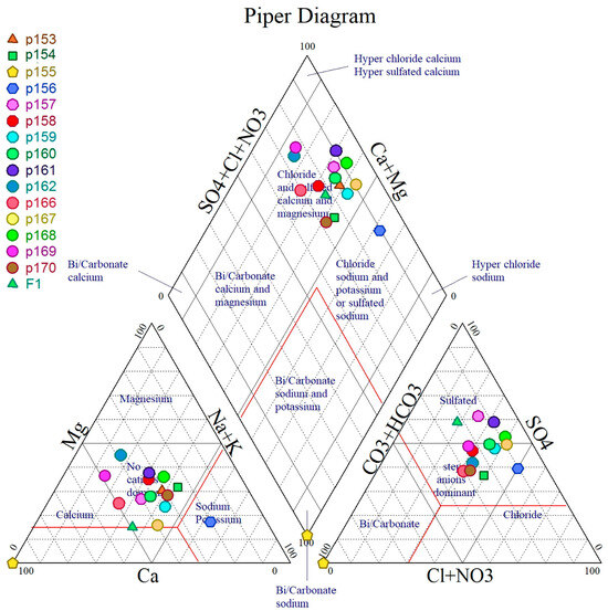
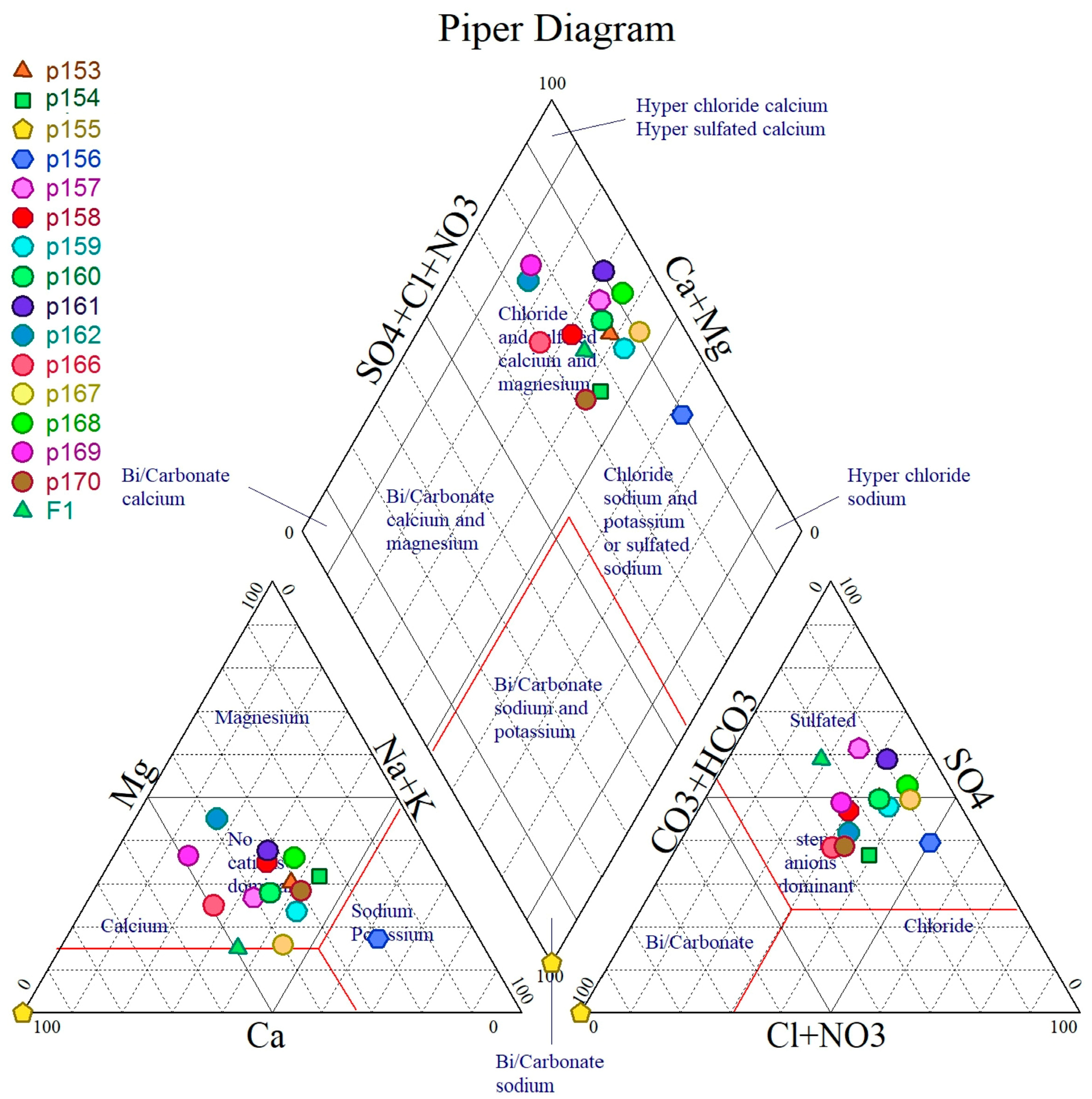
The hydrochemical investigation of groundwater samples collected from the Tabelbala Plain enabled the characterization of the aquifer system’s chemical composition and the identification of the main hydrochemical facies. This classification was based on analyses of major ion concentrations, characteristic ionic ratios, and the projection of analytical results onto a Piper diagram.
The results indicate the presence of three dominant hydrochemical facies within the study area. The sodium sulfate facies is the most prevalent, accounting for approximately 67% of the analyzed samples (119 boreholes). This facies is characterized by a relative dominance of bicarbonates over chlorides and higher calcium concentrations compared with magnesium. The calcium sulfate facies is the second most common, comprising nearly 26% of the samples (47 boreholes). It is distinguished by higher chloride concentrations relative to bicarbonates and a predominance of sodium over magnesium. The sodium chloride facies accounts for approximately 6.7% of the samples (12 boreholes). This facies is characterized by a marked dominance of sulfates over bicarbonates and higher calcium concentrations compared with magnesium (Figure 5).
Figure 5.
Piper diagram of groundwater of the study area.
3.2. Correlation Analysis of Physicochemical Parameters
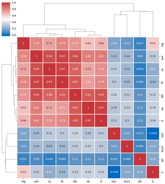
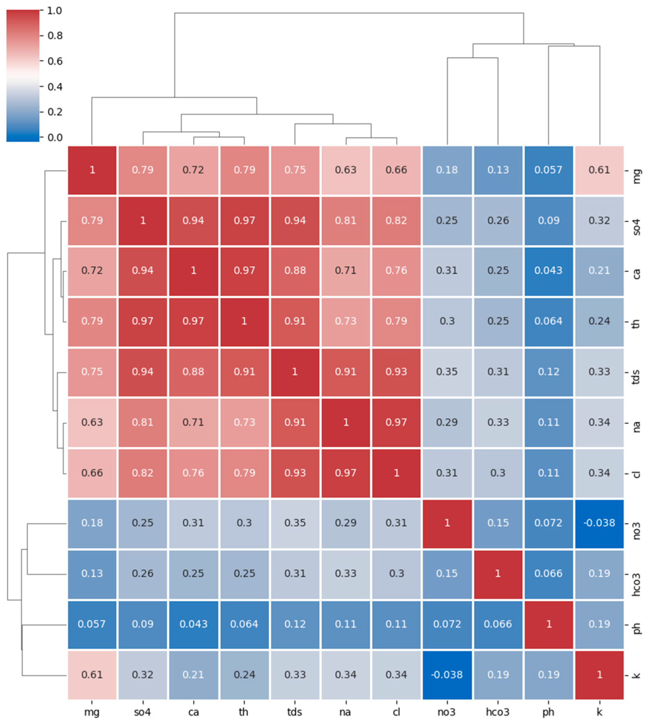
The correlation matrix analysis (Figure 6) revealed strong relationships among the main physicochemical parameters of water, allowing the identification of the dominant processes controlling water quality in the considered area. A strongly correlated group including TDS, Na+, Cl−, Ca2+, SO42−, TH, and Mg2+ was identified with very high correlation coefficients. The near-perfect correlation between Na+ and Cl− (r = 0.99) indicates that water quality is mainly controlled by the overall degree of mineralization, which is related to water–rock interactions and evaporation processes.
Figure 6.
Correlation matrix results for the 9 selected factors and the GWQI index.
Furthermore, the strong relationships between total hardness (TH) and Ca2+ (r = 0.90) and Mg2+ (r = 0.94) confirm the predominant role of carbonate formations in controlling the water’s chemical composition. Moreover, moderate correlations between NO3−, Na+, and Cl− suggest a possible anthropogenic contribution, likely associated with agricultural activities and domestic inputs. Bicarbonate ions (HCO3−) show a moderate correlation with most parameters, reflecting a mixed origin. In contrast, pH and K+ exhibit a weak correlation with all variables, indicating relative independence from mineralization processes.
3.3. Performance Analysis
The proposed methodology aims to assess water quality using three ML models predicting WQI classes: Random Forest, Support Vector Machines, and the Multi-Layer Perceptron. The performance of these models was evaluated during testing using several metrics to select the best-performing model for our full water quality datasets. Table 10 presents a static description of the different data features and the desired WQI results.
Table 10.
Descriptive statistics of physicochemical parameters of water samples.
Table 11 shows the results obtained across all testing sets, averaged over the five selected folds. It is noted that the WQI values for all samples range from 49.72 to 511.64, corresponding to four classes, good, poor, very poor, and unsustainable water quality, as shown in Table 1 (see Section WQI). Consequently, the reported precision, recall, and F1-score are averaged across all four categories and folds to yield a single score for each classifier.
Table 11.
Quantitative analysis.
From Table 11 and Table 12, we see that the RF model performs best during the test phase. It is closely followed by both ANNs and SVMs, with almost identical outcomes. The slight improvement made by the RF could be explained by the model’s ability to identify complex nonlinear relationships and its natural robustness to noisy, correlated augmented training samples. Additionally, RF performs well with data in which many features contribute weakly but jointly, and some variables are more informative than others [56,57]. Nevertheless, the performance gap remains limited, indicating that all models exhibit relatively consistent performances for the studied classification task despite differences in individual fold accuracies.
Table 12.
Confidence intervals for accuracy across all folds.
Although hydrochemical processes may involve non-linear relationships, the grid search procedure selected a linear kernel as the optimal configuration for the SVM model. This result can be explained by the relatively limited number of independent observations in the dataset (178 original samples), as the additional training points were generated through spatial interpolation and remain correlated with the original measurements. In such situations, simpler decision boundaries may yield better results than more complex kernels, such as RBF kernels, which can be prone to overfitting. Moreover, the classification problem involves 11 hydrochemical variables, and the classes appear to be reasonably separable in this feature space, allowing a linear kernel to achieve a competitive performance, comparable to that of the RF and MLP models.
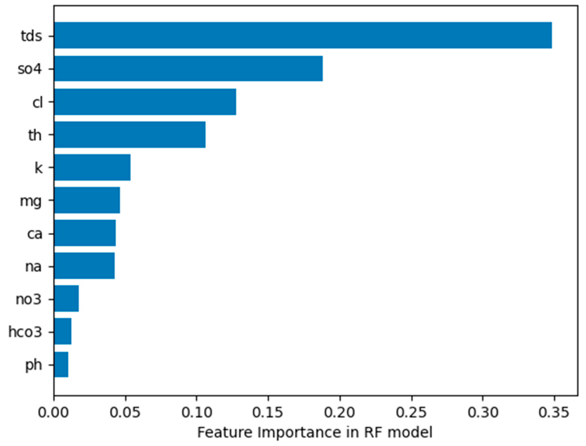
In the end, the results show that machine learning methods, thanks to their pattern recognition and modeling capabilities, are well suited for water quality assessment, achieving an overall accuracy greater than 80%. In addition to the quantitative analysis, a Permutation Feature Importance (PFI) analysis was performed on the test data. By randomly permuting feature columns, the PFI breaks the relationship between the inputs and the target to determine how much the model relies on particular features [58].
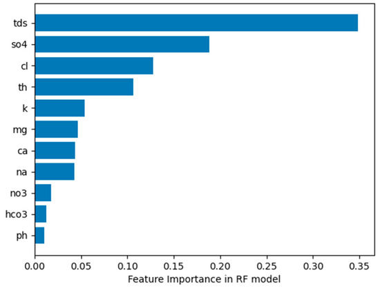
Compared to the initial dataset, Figure 7 illustrates the relative importance of the physicochemical parameters as captured by the Random Forest model. Parameters such as TDS, SO42−, TH, and Cl− had higher feature importance values, indicating stronger contributions to predicting WQI classes. Other factors, including pH, HCO3−, and NO3−, were assigned lower importance, indicating a smaller influence on the model’s predictions. These results generally align with the WHO-recommended parameter weights, except for NO3−. Although nitrate is critical from a public health perspective, its feature importance in the Random Forest model reflects its predictive contribution to the model, not its regulatory significance. As shown in Table 1, NO3− exhibits a standard deviation of 20.62 mg/L and a range of 6–135 mg/L, which is substantially lower than SO42− (STD = 340.94 mg/L) and Cl− (STD = 223.03 mg/L). This limited variability likely reduced its discriminative power in the classification task. Furthermore, as shown in the correlation matrix (Figure 6), moderate correlations between NO3−, Na+, and Cl− suggest that its predictive information may be partially captured by these more variable and correlated parameters.
Figure 7.
Permutation importance for RF on testing data.
Due to the limited number of original groundwater samples (178 instances), no comparison with models trained exclusively on the original observations was conducted. With only 178 samples split into five folds, each training fold would contain approximately 35–37 original instances, which is insufficient for stable multi-class learning across four WQI categories and likely to yield unreliable results that are not directly comparable to those of the augmented models. This constitutes a recognized limitation, and such a comparison is planned for future work when a larger dataset becomes available.
A computational time comparison was performed for each classifier, as reported in Table 13. All experiments were conducted on a personal laptop equipped with an Intel i7 CPU and 16 GB RAM using the Python programming environment and the Scikit-learn library. No GPU acceleration was used.
Table 13.
Computational time.
The results indicate that all machine learning models achieve efficient performances for water quality assessment, with both predictive capability and runtime. The SVM model achieved the lowest average runtime across all folds (0.013 s), followed by the Random Forest classifier. Nevertheless, the computational time required by RF remained negligible and does not limit its practical applicability, particularly considering that it achieved the highest predictive accuracy among the evaluated models.
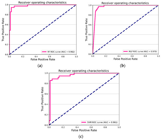
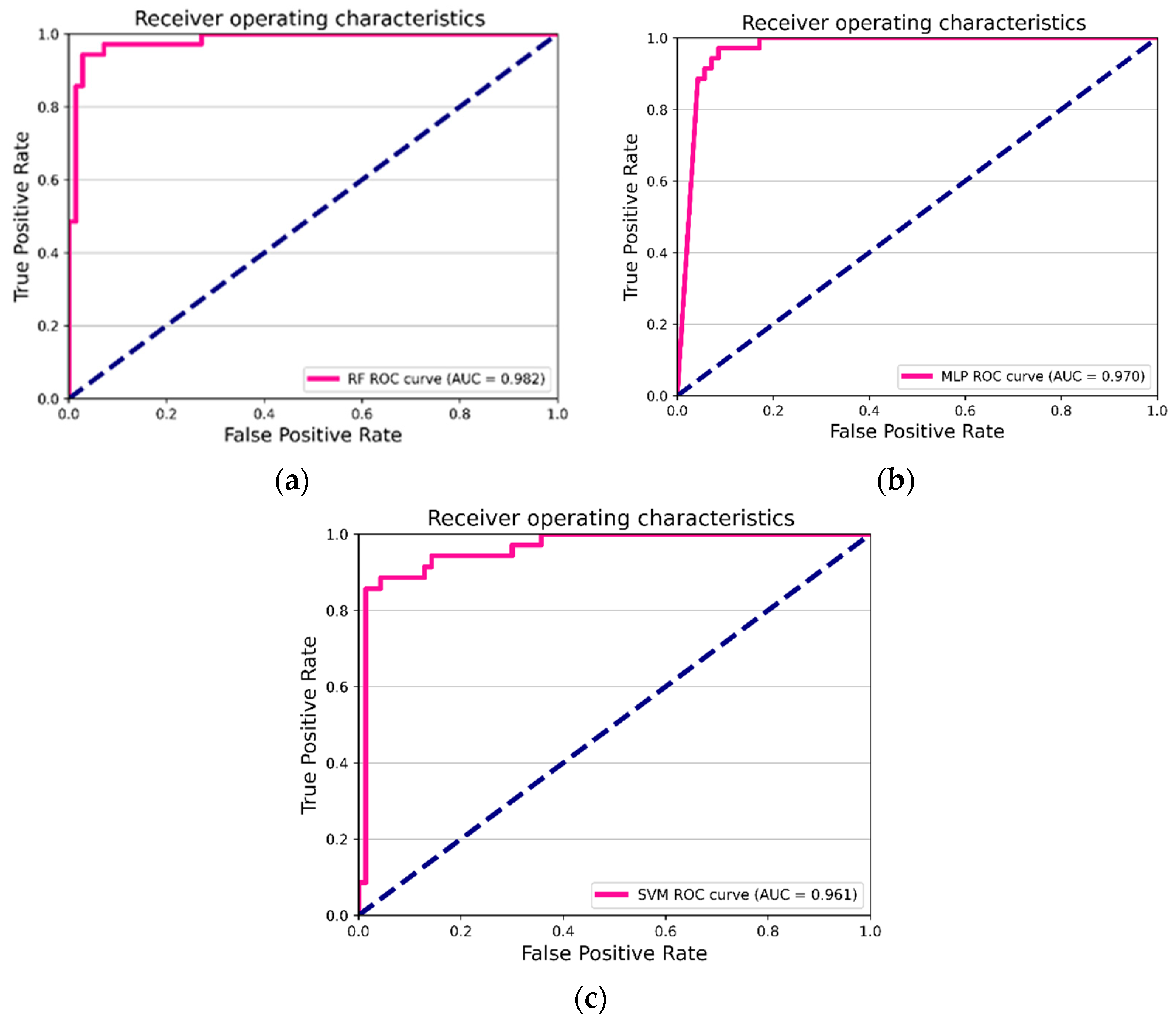
The superiority of the RF is further established by the ROC-AUC curve, which shows an AUC of 0.982, demonstrating an excellent classifier performance. Both ANNs and SVMs show excellent results, with AUC values of 0.97 and 0.961, respectively (Figure 8).
Figure 8.
The ROC-AUC curve for (a) RF, (b) ANNs, (c) SVMs.
However, the extremely high AUC observed is likely influenced by the large number of correlated augmented training samples, which reduces model uncertainty and can artificially inflate apparent predictive performance. However, evaluation was performed exclusively on independent, original samples. Yet, given the isolated character of the studied region and the limited information available, the proposed study remains a valuable tool for further experimentation and potentially for narrowing the search region.
3.4. Water Quality Mapping and Spatial Distribution
During the performance analysis (Table 10), we noticed that the calculated WQI values using all selected factors and generated samples range from around 50 to 511, indicating a water quality classified from unsustainable to good. In addition, the vast majority of water points have poor to very poor water quality.
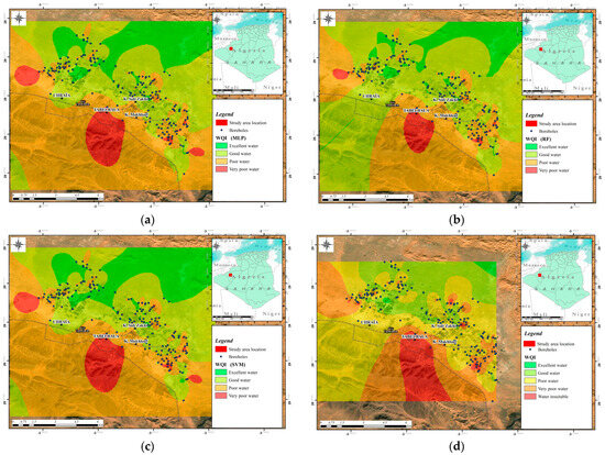
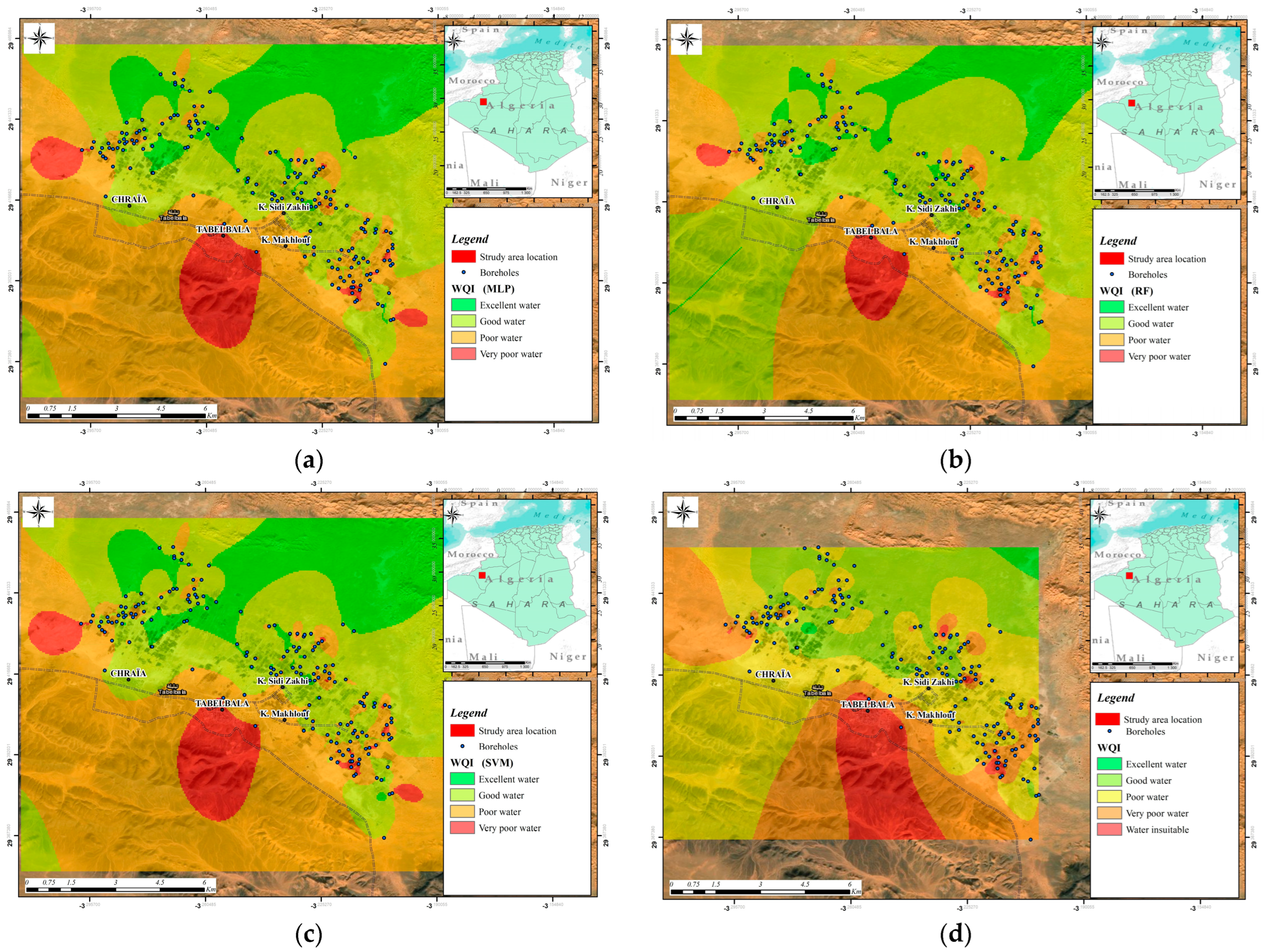
According to the ANRH, the Tabelbala region experienced a noticeable decrease in groundwater piezometric levels [59]. Bennia, Kebir, Talhi, Zeroual and Djerida [5] link these observations to a significant disturbance of the hydrochemical aspects of these sources, ultimately resulting in lower water quality. Figure 9 illustrates the spatial distribution of groundwater quality classes across the study area as predicted by the three machine learning classifiers (Figure 9a–c). Although the models achieved comparable predictive performances (with accuracies of 80–90%), some differences in spatial distribution were observed, particularly with the Random Forest classifier. The reliability of the produced maps strongly depends on both the quantity and quality of available data. Consequently, predictions located near sampling points are expected to be more reliable than those farther from the original observations, given the potential spatial variability of groundwater quality. The use of a limited interpolation radius (150 m) during the augmentation phase and the integration of original samples helped preserve local variability and improve the spatial consistency of the predicted maps within the study area.
Figure 9.
Spatial distribution of WQI classes in the Tabelbala study area as predicted by (a) Multi-Layer Perceptron (MLP), (b) Random Forest (RF), (c) Support Vector Machines (SVMs), compared with (d) the spatial interpolation of WQI values calculated directly from the original 178 samples.
In addition, a comparison is made with the interpolation of WQI values calculated directly on initial data (178 samples). Here, again, the RF shows the greatest similarity to the conventional technique. On the other hand, both ANNs and SVMs return almost similar results. Despite a slight difference in accuracy compared to the RF, both fail to separate certain poor-water-quality class entities.
Finally, we can notice that Figure 9d initially indicated the presence of an additional class corresponding to excellent water quality. However, only two samples belonged to this category, which represents an extremely small proportion of the dataset. To avoid instability during model training and classification, this class was excluded during post-processing, leaving 176 instances for the subsequent augmentation and modeling steps. Removing this class may slightly modify the original class distribution.
4. Conclusions
In this study, a framework integrating the Water Quality Index (WQI) with IDW-based spatial data augmentation and three machine learning classifiers—Random Forest (RF), Support Vector Machines (SVMs), and Artificial Neural Networks (ANNs)—was developed and evaluated for groundwater quality assessment in the hyper-arid desert region of Tabelbala, southwestern Algeria. Conducting such assessments in remote arid regions remains a significant challenge due to limited field sample availability, the high cost of hydrochemical analyses, and the remoteness of sampling sites. The proposed methodology was specifically designed to address these constraints and to provide local authorities and water resource managers with a reliable, data-driven decision-support tool adapted to data-scarce environments.
The main findings of this study can be summarized as follows. Starting from 178 original groundwater samples, IDW interpolation with a sensitivity-optimized 150 m radius generated 2779 augmented training points, substantially improving model training stability. Random Forest achieved the highest predictive accuracy (85.9%), followed by ANN (84.7%) and SVM (83.1%), with all models demonstrating excellent discriminative performances (ROC-AUC > 0.96). Permutation Feature Importance analysis identified TDS, SO42−, TH, and Cl− as the most influential parameters, consistent with WHO recommendations. The generated spatial distribution maps revealed that the majority of groundwater sources in the study area exhibit poor to very poor quality, confirming the piezometric level regressions previously reported by the ANRH. These findings carry direct and urgent implications for local water governance in Tabelbala. Local authorities should prioritize the installation of point-of-use treatment systems across the identified high-risk zones, establish a systematic borehole monitoring network to track water quality evolution over time, and implement targeted community awareness programs to inform residents of the health risks associated with consuming untreated groundwater. The proposed framework provides water resource managers with the spatial and predictive information needed to guide these interventions effectively and allocate resources to the most critical areas first.
Despite these promising results, several limitations must be acknowledged. The testing set per fold comprised only 32–37 original samples, limiting the ability to fully assess model generalization beyond the Tabelbala region. As IDW generates highly correlated synthetic observations that do not introduce independent variability, the reported performance metrics should be interpreted as upper-bound estimates. In addition, no formal spatial autocorrelation test was applied to the residuals, and the random cross-validation strategy does not ensure full spatial independence between the training and test samples. Finally, no direct comparison with models trained exclusively on the original, unaugmented dataset was conducted, as the available sample size per fold would be insufficient for stable multi-class training.
Future research should address these limitations by incorporating spatial cross-validation strategies, such as block-based or distance-based splitting, as larger, more spatially distributed datasets become available. The integration of remote sensing data, the exploration of advanced deep learning architectures such as Convolutional Neural Networks, the inclusion of seasonal and temporal variations in water quality, and a direct ablation study comparing augmented versus non-augmented model performance are identified as key directions for extending this work. The methodology is also transferable to other arid and semi-arid regions of Algeria and beyond facing similar data scarcity challenges.
The results of this study send a clear and urgent message to local water authorities in Tabelbala. The spatial maps produced by the three classifiers consistently identify specific zones where groundwater quality is classified as very poor or unsustainable for consumption. Water managers should use these maps as a prioritization tool to concentrate immediate action where it is most needed. In practical terms, this means deploying affordable treatment solutions such as reverse osmosis or solar disinfection units at the most critical boreholes, establishing a regular sampling and monitoring schedule to detect quality degradation early, and engaging local communities through awareness campaigns that explain the health risks of consuming untreated groundwater. Policymakers at the regional and national level should also consider this methodology as a replicable template for other undermonitored arid zones across Algeria, where similar data scarcity challenges prevent conventional water quality assessments.
The proposed framework represents a computationally efficient and replicable contribution to groundwater quality assessment in data-limited environments, directly supporting the United Nations Sustainable Development Goals, particularly SDG 6 (Clean Water and Sanitation), SDG 13 (Climate Action), and SDG 17 (Partnerships for the Goals), by advancing evidence-based water resource management and promoting open, transferable methodologies for global water security.
Author Contributions
Conceptualization, N.F., L.W.K. and A.D. (Abdessamed Derdour); methodology, N.F., A.B., L.W.K. and A.D. (Abdessamed Derdour); software, N.F. and A.D. (Achraf Djerida); validation, N.F., A.B. and H.A.; formal analysis, N.F., A.D. (Achraf Djerida) and H.A.; investigation, N.F. and S.K.; resources, M.A.-M. and H.A.; data curation, N.F.; writing—original draft preparation, N.F. and A.D. (Achraf Djerida); writing—review and editing, N.F., A.D. (Abdessamed Derdour), A.B., M.A.-M. and H.A.; visualization, N.F., A.B., L.W.K. and A.D. (Achraf Djerida); supervision, A.D. (Abdessamed Derdour); project administration, A.D. (Abdessamed Derdour) and M.A.-M.; funding acquisition, M.A.-M. and A.D. (Abdessamed Derdour). All authors have read and agreed to the published version of the manuscript.
Funding
This research was funded by Princess Nourah bint Abdulrahman University Researchers Supporting Project number (PNURSP2026R241), Princess Nourah bint Abdulrahman University, Riyadh, Saudi Arabia.
Institutional Review Board Statement
Not applicable.
Informed Consent Statement
Not applicable.
Data Availability Statement
The original contributions presented in this study are included in the article. Further inquiries can be directed to the corresponding author.
Acknowledgments
Princess Nourah bint Abdulrahman University Researchers Supporting Project number (PNURSP2026R241), Princess Nourah bint Abdulrahman University, Riyadh, Saudi Arabia.
Conflicts of Interest
The authors declare no conflicts of interest.
Abbreviations
The following abbreviations are used in this manuscript:
| ANNs | Artificial Neural Networks |
| AUC | Area Under the Curve |
| CV | Cross-Validation |
| GIS | Geographic Information System |
| GPS | Global Positioning System |
| IDW | Inverse Distance Weighting |
| ML | Machine Learning |
| MLP | Multi-Layer Perceptron |
| PFI | Permutation Feature Importance |
| RF | Random Forest |
| RMSE | Root Mean Square Error |
| ROC | Receiver Operating Characteristic |
| SDG | Sustainable Development Goal |
| STD | Standard Deviation |
| SVMs | Support Vector Machines |
| TDS | Total Dissolved Solids |
| TH | Total Hardness |
| WHO | World Health Organization |
| WQI | Water Quality Index |
References
- Asadi, E.; Isazadeh, M.; Samadianfard, S.; Ramli, M.F.; Mosavi, A.; Nabipour, N.; Shamshirband, S.; Hajnal, E.; Chau, K.-W. Groundwater quality assessment for sustainable drinking and irrigation. Sustainability 2019, 12, 177. [Google Scholar] [CrossRef] [Scilit]
- Wang, X. Managing land carrying capacity: Key to achieving sustainable production systems for food security. Land 2022, 11, 484. [Google Scholar] [CrossRef] [Scilit]
- Gerten, D.; Heck, V.; Jägermeyr, J.; Bodirsky, B.L.; Fetzer, I.; Jalava, M.; Kummu, M.; Lucht, W.; Rockström, J.; Schaphoff, S. Feeding ten billion people is possible within four terrestrial planetary boundaries. Nat. Sustain. 2020, 3, 200–208. [Google Scholar] [CrossRef] [Scilit]
- Aslam, R.A.; Shrestha, S.; Pandey, V.P. Groundwater vulnerability to climate change: A review of the assessment methodology. Sci. Total Environ. 2018, 612, 853–875. [Google Scholar] [CrossRef] [Scilit] [PubMed]
- Bennia, A.; Kebir, L.W.; Talhi, A.; Zeroual, I.; Djerida, A. Groundwater Quality Assessments for Drinking Purposes Based On WQI And GIS In the Plain of Tabelbala, South-West Algeria. In Proceedings of the 2024 IEEE Mediterranean and Middle-East Geoscience and Remote Sensing Symposium (M2GARSS), Oran, Algeria, 15–17 April 2024; pp. 168–172. [Google Scholar]
- M’nassri, S.; El Amri, A.; Nasri, N.; Majdoub, R. Estimation of irrigation water quality index in a semi-arid environment using data-driven approach. Water Supply 2022, 22, 5161–5175. [Google Scholar] [CrossRef] [Scilit]
- Banda, T.D.; Muthukrishnavellaisamy, K. Review of the existing water quality indices (WQIs). Pollut. Res. 2020, 39, 489–514. [Google Scholar]
- Moudou, M.; El Hammoudani, Y.; Haboubi, K.; Achoukhi, I.; El Boudammoussi, M.; Faiz, H.; Touzani, A.; Dimane, F. Water quality indices (WQIs): An in-depth analysis and overview. In Proceedings of the 4th Edition of Oriental Days for the Environment (JOE4), Oujda, Morocco, 24 May 2024; p. 02015. [Google Scholar]
- Elkhalki, S.; Hamed, R.; Jodeh, S.; Ghalit, M.; Elbarghmi, R.; Azzaoui, K.; Hanbali, G.; Ben Zhir, K.; Ait Taleb, B.; Zarrouk, A. Study of the quality index of groundwater (GWQI) and its use for irrigation purposes using the techniques of the geographic information system (GIS) of the plain Nekor-Ghiss (Morocco). Front. Environ. Sci. 2023, 11, 1179283. [Google Scholar] [CrossRef] [Scilit]
- Houari, I.M.; Bouselsal, B.; Lakhdari, A.S. Evaluating groundwater potability and health risks from nitrates in the semi-arid region of Algeria. Ecol. Eng. Environ. Technol. 2024, 25, 220–233. [Google Scholar] [CrossRef] [Scilit]
- De León, G.S.; Ramos-Leal, J.A.; Ramírez, J.M.; Almanza-Tovar, O.G. Drought and Water Quality in a Semi-arid Area: Effects in Livestock Production, Agriculture and Use Urban. Water Resour. Manag. 2025, 39, 1605–1621. [Google Scholar] [CrossRef] [Scilit]
- Ahmad, T.; Ali, L.; Alshamsi, D.; Aldahan, A.; El-Askary, H.; Ahmed, A. AI-powered water quality index prediction: Unveiling machine learning precision in hyper-arid regions. Earth Syst. Environ. 2025, 9, 677–694. [Google Scholar] [CrossRef] [Scilit]
- Hamlat, A.; Guidoum, A. Assessment of groundwater quality in a semiarid region of Northwestern Algeria using water quality index (WQI). Appl. Water Sci. 2018, 8, 220. [Google Scholar] [CrossRef] [Scilit]
- FAO Aquastat. FAO’s Global Information System on Water and Agriculture; FAO: Rome, Italy, 2020. [Google Scholar]
- Turdaliev, A.; Yo Darmonov, D.; Teshaboyev, N.; Saminov, A.; Abdurakhmonova, M. Influence of irrigation with salty water on the composition of absorbed bases of hydromorphic structure of soil. In Proceedings of the IOP Conference Series: Earth and Environmental Science, Tashkent, Uzbekistan, 18–19 March 2022; p. 012047. [Google Scholar]
- Ur Rehman, Z.; Aziz, Z.; Khalid, U.; Ijaz, N.; ur Rehman, S.; Ijaz, Z. Artificial intelligence-driven enhanced CBR modeling of sandy soils considering broad grain size variability. J. Rock Mech. Geotech. Eng. 2025, 17, 3161–3179. [Google Scholar] [CrossRef] [Scilit]
- Parmar, A.; Katariya, R.; Patel, V. A review on random forest: An ensemble classifier. In Proceedings of the International Conference on Intelligent Data Communication Technologies and Internet of Things, Coimbatore, India, 7–8 August 2018; pp. 758–763. [Google Scholar]
- Derdour, A.; Jodar-Abellan, A.; Pardo, M.Á.; Ghoneim, S.S.; Hussein, E.E. Designing efficient and sustainable predictions of water quality indexes at the regional scale using machine learning algorithms. Water 2022, 14, 2801. [Google Scholar] [CrossRef] [Scilit]
- Zou, J.; Han, Y.; So, S.-S. Overview of artificial neural networks. Artif. Neural Netw. Methods Appl. 2009, 458, 14–22. [Google Scholar]
- Han, Z.; Zhang, S.; He, L. Predicting and investigating water quality index by robust machine learning methods. J. Environ. Manag. 2025, 381, 125156. [Google Scholar] [CrossRef] [Scilit]
- Cymes, I.; Glińska-Lewczuk, K. The use of water quality indices (WQI and SAR) for multipurpose assessment of water in dam reservoirs. J. Elem. 2016, 21, 1211–1224. [Google Scholar]
- Meireles, A.C.M.; Andrade, E.M.d.; Chaves, L.C.G.; Frischkorn, H.; Crisostomo, L.A. A new proposal of the classification of irrigation water. Rev. Ciência Agronômica 2010, 41, 349–357. [Google Scholar] [CrossRef] [Scilit]
- Wang, X.; Zhang, F.; Ding, J. Evaluation of water quality based on a machine learning algorithm and water quality index for the Ebinur Lake Watershed, China. Sci. Rep. 2017, 7, 12858. [Google Scholar] [CrossRef] [Scilit]
- Lee, J.; Lee, J.; Lee, M.; Lee, M.; Kim, Y.; Hyung, J.; Kim, K.; Cha, Y.; Koo, J. Development of a short-term water quality prediction model for urban rivers using real-time water quality data. Water Supply 2022, 22, 4082–4097. [Google Scholar] [CrossRef] [Scilit]
- Mumuni, A.; Mumuni, F. Data augmentation with automated machine learning: Approaches and performance comparison with classical data augmentation methods. Knowl. Inf. Syst. 2025, 67, 4035–4085. [Google Scholar] [CrossRef] [Scilit]
- Shepard, D. A two-dimensional interpolation function for irregularly-spaced data. In Proceedings of the 1968 23rd ACM National Conference, Princeton, NJ, USA, 27–29 August 1968; pp. 517–524. [Google Scholar]
- Ijaz, N.; Ijaz, Z.; Zhou, N.; Ijaz, H.; Ijaz, A. Advanced Geospatial Modeling of Highly Variable Geotechnical Data for Infrastructure Resilience. Bull. Eng. Geol. Environ. 2026, 85, 145. [Google Scholar] [CrossRef] [Scilit]
- Naidu, G.; Zuva, T.; Sibanda, E.M. A review of evaluation metrics in machine learning algorithms. In Proceedings of the Computer Science On-Line Conference, Online, 3–5 April 2023; pp. 15–25. [Google Scholar]
- Kaddoura, S. Evaluation of machine learning algorithm on drinking water quality for better sustainability. Sustainability 2022, 14, 11478. [Google Scholar] [CrossRef] [Scilit]
- Tilmatine, M. Un parler berbéro-songhay du sud-ouest algérien (Tabelbala): Éléments d’histoire et de linguistique. Etudes Doc. Berbères 1996, 14, 163–197. [Google Scholar] [CrossRef] [Scilit]
- Merzougui, T.; Bouanani, A.; Rezzoug, C.; Mekkaoui, A.; Hamzaoui, F.A.; Merzougui, F.Z. Palm grove groundwater assessment and hydrodynamic modelling Case study: Beni Abbes, South-West of Algeria. J. Water Land Dev. 2019, 43, 133–143. [Google Scholar] [CrossRef] [Scilit]
- Merzougui, T. Overview of the Hydrogeology of a Fractured Bedrock Aquifer. Chain of Ougarta the Saoura—South-west Algeria. Larhyss J. 2022, 19, 33–55. [Google Scholar]
- Kharroubi, M.; Bouselsal, B.; Ouarekh, M.; Benaabidate, L.; Khadri, R. Water quality assessment and hydrogeochemical characterization of the Ouargla complex terminal aquifer (Algerian Sahara). Arab. J. Geosci. 2022, 15, 251. [Google Scholar] [CrossRef] [Scilit]
- Edition, F. Guidelines for drinking-water quality. WHO Chron. 2011, 38, 104–108. [Google Scholar]
- Lokman, A.; Ismail, W.Z.W.; Aziz, N.A.A. A review of water quality forecasting and classification using machine learning models and statistical analysis. Water 2025, 17, 2243. [Google Scholar] [CrossRef] [Scilit]
- Benmoshe, N. A simple solution for the inverse distance weighting interpolation (IDW) clustering problem. Science 2025, 7, 30. [Google Scholar] [CrossRef] [Scilit]
- Yang, W.; Zhao, Y.; Wang, D.; Wu, H.; Lin, A.; He, L. Using principal components analysis and IDW interpolation to determine spatial and temporal changes of surface water quality of Xin’anjiang river in Huangshan, China. Int. J. Environ. Res. Public Health 2020, 17, 2942. [Google Scholar] [CrossRef] [Scilit]
- Charizopoulos, N.; Zagana, E.; Psilovikos, A. Assessment of natural and anthropogenic impacts in groundwater, utilizing multivariate statistical analysis and inverse distance weighted interpolation modeling: The case of a Scopia basin (Central Greece). Environ. Earth Sci. 2018, 77, 380. [Google Scholar] [CrossRef] [Scilit]
- Hua, A.; Baharudin, M.; Ngadiran, S.; Sulaiman, S. Integrated Principal Component Analysis (pca) and Inverse Distance Weighted (IDW) Modeling for Water Quality Assessment in the Melaka River Basin. Appl. Ecol. Environ. Res. 2025, 23, 10315–10332. [Google Scholar] [CrossRef] [Scilit]
- Wackernagel, H. Multivariate Geostatistics: An Introduction with Applications; Springer Science & Business Media: Berlin/Heidelberg, Germany, 2003. [Google Scholar]
- Djerida, A.; Bennia, A.; Kebir, L.W. Groundwater potential mapping in the plain of Sidi Bel Abbes, Algeria, using remote sensing, neighboring data, and robust machine learning. Arab. J. Geosci. 2023, 16, 325. [Google Scholar] [CrossRef] [Scilit]
- Gorriz, J.M.; Clemente, R.M.; Segovia, F.; Ramirez, J.; Ortiz, A.; Suckling, J. Is K-fold cross validation the best model selection method for Machine Learning? arXiv 2024, arXiv:2401.16407. [Google Scholar] [CrossRef] [Scilit]
- Elgeldawi, E.; Sayed, A.; Galal, A.R.; Zaki, A.M. Hyperparameter tuning for machine learning algorithms used for arabic sentiment analysis. Informatics 2021, 8, 79. [Google Scholar] [CrossRef] [Scilit]
- Bernett, J.; Blumenthal, D.B.; Grimm, D.G.; Haselbeck, F.; Joeres, R.; Kalinina, O.V.; List, M. Guiding questions to avoid data leakage in biological machine learning applications. Nat. Methods 2024, 21, 1444–1453. [Google Scholar] [CrossRef] [Scilit]
- Qian, Y.; Zhou, W.; Yan, J.; Li, W.; Han, L. Comparing machine learning classifiers for object-based land cover classification using very high resolution imagery. Remote Sens. 2014, 7, 153–168. [Google Scholar] [CrossRef] [Scilit]
- Thanh Noi, P.; Kappas, M. Comparison of random forest, k-nearest neighbor, and support vector machine classifiers for land cover classification using Sentinel-2 imagery. Sensors 2017, 18, 18. [Google Scholar] [CrossRef] [Scilit]
- Uddin, G.; Nash, S.; Olbert, A.I. Optimization of parameters in a water quality index model using principal component analysis. In Proceedings of the 39th IAHR World Congress, Granada, Spain, 19–24 June 2022; p. 24. [Google Scholar]
- Adugna, T.; Xu, W.; Fan, J. Comparison of random forest and support vector machine classifiers for regional land cover mapping using coarse resolution FY-3C images. Remote Sens. 2022, 14, 574. [Google Scholar] [CrossRef] [Scilit]
- Dewi, D.A.; Wei, A.S.; Lin, L.C.; Heng, C.D. Water quality prediction using random forest algorithm and optimization. J. Appl. Data Sci. 2024, 5, 1354–1362. [Google Scholar] [CrossRef] [Scilit]
- Budak, İ. Prediction of Water Quality’s pH value using Random Forest and LightGBM Algorithms. MEMBA Su Bilim. Derg. 2025, 11, 42–49. [Google Scholar] [CrossRef] [Scilit]
- Abobakr Yahya, A.S.; Ahmed, A.N.; Binti Othman, F.; Ibrahim, R.K.; Afan, H.A.; El-Shafie, A.; Fai, C.M.; Hossain, M.S.; Ehteram, M.; Elshafie, A. Water quality prediction model based support vector machine model for ungauged river catchment under dual scenarios. Water 2019, 11, 1231. [Google Scholar] [CrossRef] [Scilit]
- Riaz, M.T.; Riaz, M.T.; Rehman, A.; Bindajam, A.A.; Mallick, J.; Abdo, H.G. An integrated approach of support vector machine (SVM) and weight of evidence (WOE) techniques to map groundwater potential and assess water quality. Sci. Rep. 2024, 14, 26186. [Google Scholar] [CrossRef] [Scilit] [PubMed]
- Palabıyık, S.; Akkan, T. Evaluation of water quality based on artificial intelligence: Performance of multilayer perceptron neural networks and multiple linear regression versus water quality indexes. Environ. Dev. Sustain. 2024, 28, 2717–2724. [Google Scholar] [CrossRef] [Scilit]
- Wu, J.; Wang, Z. A hybrid model for water quality prediction based on an artificial neural network, wavelet transform, and long short-term memory. Water 2022, 14, 610. [Google Scholar] [CrossRef] [Scilit]
- Narkhede, S. Understanding auc-roc curve. Data Sci. 2018, 26, 220. [Google Scholar]
- Reif, D.M.; Motsinger, A.A.; McKinney, B.A.; Crowe, J.E.; Moore, J.H. Feature selection using a random forests classifier for the integrated analysis of multiple data types. In Proceedings of the 2006 IEEE Symposium on Computational Intelligence and Bioinformatics and Computational Biology, Toronto, ON, Canada, 28–29 September 2006; pp. 1–8. [Google Scholar]
- Nguyen, T.-T.; Huang, J.Z.; Nguyen, T.T. Unbiased feature selection in learning random forests for high-dimensional data. Sci. World J. 2015, 2015, 471371. [Google Scholar] [CrossRef] [Scilit]
- Arunthavanathan, R.; Khan, F.; Ahmed, S.; Imtiaz, S. Autonomous fault diagnosis and root cause analysis for the processing system using one-class SVM and NN permutation algorithm. Ind. Eng. Chem. Res. 2022, 61, 1408–1422. [Google Scholar] [CrossRef] [Scilit]
- Bennia, A.; Zeroual, I.; Talhi, A.; Kebir, L.W. Groundwater potential mapping using the integration of AHP method, GIS and remote sensing: A case study of the Tabelbala region, Algeria. Bull. Miner. Res. Explor. 2023, 172, 41–60. [Google Scholar] [CrossRef] [Scilit]

Disclaimer/Publisher’s Note: The statements, opinions and data contained in all publications are solely those of the individual author(s) and contributor(s) and not of MDPI and/or the editor(s). MDPI and/or the editor(s) disclaim responsibility for any injury to people or property resulting from any ideas, methods, instructions or products referred to in the content. |
© 2026 by the authors. Licensee MDPI, Basel, Switzerland. This article is an open access article distributed under the terms and conditions of the Creative Commons Attribution (CC BY) license.