


Abstract
The rapid expansion of e-commerce and on-demand logistics has intensified the need for cost-effective and reliable urban distribution systems. This paper investigates an energy-aware routing problem for electric vehicle fleets operating from multiple depots under time-varying traffic conditions. We propose a novel multi-depot vehicle routing model that jointly incorporates time-dependent travel speeds, simultaneous pickup and delivery operations, and time window constraints. The model explicitly captures key operational realities, including battery capacity limitations, load- and speed-dependent energy consumption, synchronized pickup-delivery requirements, and soft time windows. The objective is to minimize total operational cost by simultaneously optimizing depot assignments, vehicle routes, and service schedules. Given the NP-hard nature of the problem, we develop a two-stage heuristic solution framework. In the first stage, a spatio-temporal clustering strategy is employed to assign customers to depots efficiently. In the second stage, route construction and improvement are performed using an enhanced Adaptive Large Neighborhood Search (ALNS) algorithm equipped with problem-specific destroy and repair operators. Computational experiments on adapted benchmark instances demonstrate that the proposed approach consistently produces high-quality solutions and exhibits robust convergence behavior. In addition, sensitivity analyses provide managerial insights, revealing an optimal range of vehicle energy capacity and an economically efficient speed band that balances travel time and energy consumption.
1. Introduction
The expansion of China’s logistics industry is closely tied to the sustained growth in express delivery volume. As reported by the China Federation of Logistics and Purchasing (2025), the total value of social logistics reached 360.6 trillion yuan in 2024, reflecting a year-on-year increase of 5.8% Although the logistics sector has consistently pursued cost reduction and efficiency improvement in recent years, challenges such as high logistics costs and low efficiency in certain areas persist, exacerbated by deepening economic integration and intensifying market competition. These issues hinder the industry’s ability to meet the development requirements for high-quality and high-efficiency logistics distribution. Transportation, being the core activity in logistics, directly determines both logistics costs and service levels through the optimization of its distribution schemes.
The Vehicle Routing Problem (VRP), first introduced by Dantzig and Ramser in 1959 [1], has since become a fundamental theoretical cornerstone for logistics distribution optimization and has been extensively studied in academia [2,3,4]. The problem aims to optimally arrange the sequence for vehicles to serve customers, achieving the best configuration between vehicles and clients while minimizing distribution costs under various service constraints. Over the past six decades, the classical VRP has evolved into a rich family of variants to address increasingly complex and realistic logistics scenarios. A prominent extension is the multi-depot VRP (MDVRP), where customers are served from multiple depots [5,6,7]. This formulation challenges the optimization process to simultaneously determine depot assignments and vehicle routes, aiming to minimize total cost while balancing workloads across facilities. Another significant variant is the VRP with pickup and delivery (VRPPD), which models real-world operations in which goods must be transported from pickup points to delivery locations, often under precedence or pairing constraints [8,9,10]. This problem captures the essence of reverse logistics and last-mile delivery, with solution methods focusing on efficient route construction and load management to avoid unnecessary detours.
In recent years, driven by global sustainability goals, the electric VRP (EVRP) has emerged as a critical research stream. A core challenge in EVRP is accurately modeling and optimizing energy consumption, which depends not only on travel distance but also on vehicle load, road gradient, and-importantly-driving speed. Researchers have developed various energy-estimation models, ranging from linear approximations to more sophisticated physics-based formulations, to integrate battery capacity and charging dynamics into route planning [10,11]. Building on this, the time-dependent VRP (TDVRP) introduces variable travel speeds across different periods of the day (e.g., peak versus off-peak hours), making travel times and consequently energy consumption dependent on the time of service. Studies in this area often incorporate speed profiles or historical traffic data to reflect urban congestion patterns, aiming to identify routes that minimize time or energy under fluctuating conditions [12,13,14]. Collectively, these advances provide a growing theoretical toolkit for greening urban freight distribution.
However, the existing literature tends to address these dimensions in relative isolation. Most studies focus on combining only two or three aspects-for example, electric vehicles with time windows, or multi-depot problems with pickup and delivery-while a holistic model that simultaneously integrates multi-depot operations, electric-vehicle range limitations, load-capacity constraints, time-dependent speeds, and simultaneous pickup–delivery tasks remains largely unexplored. In practical urban logistics, these factors are deeply intertwined: the choice of depot affects initial load and route distance; vehicle speed in traffic influences energy drain and service time; and the interplay of pickups and deliveries shapes load fluctuations along a route. Ignoring their synergy can lead to models that are either oversimplified or operationally impractical. Therefore, developing a comprehensive optimization framework that captures these interdependent constraints is crucial for generating realistic, cost-effective, and executable distribution plans in complex urban environments.
To address this research gap, this paper proposes an Energy-Aware Vehicle Routing Problem with Pickup–Delivery and Time Windows (EA-VRPPDTW) model that comprehensively integrates multiple critical dimensions. The model is specifically designed for multi-depot collaborative distribution in time-dependent road networks, simultaneously encompassing bidirectional logistics tasks (simultaneous pickup and delivery), soft time window constraints (reflected via penalty functions), vehicle load capacity limits, and a speed- and load-sensitive energy consumption model. To tackle this complex NP-hard problem, we design a novel Two-Stage Heuristic (TSH) algorithm. This algorithm integrates spatio-temporal aware clustering for intelligent customer grouping in the first stage, followed by an enhanced Adaptive Large Neighborhood Search (ALNS) mechanism in the second stage for route refinement and optimization. By leveraging a spatio-temporal distance metric and incorporating a phased dynamic initialization process with adaptive collaborative optimization, the TSH algorithm offers an effective solution approach for the efficient operation of multi-depot electric vehicle collaborative distribution in urban settings.
The remainder of this paper is organized as follows: Section 2 provides a comprehensive literature review. Section 3 states the research objectives and develops the mathematical model. Section 4 details the proposed Two-Stage Heuristic algorithm. Section 5 presents the experimental design and analyzes the results. Finally, Section 6 summarizes the main findings and outlines directions for future research.
2. Literature Review
Since its inception, the VRP has been extensively studied and extended to address a wide range of real-world logistics challenges. This section reviews two key research streams directly relevant to the present study: multi-depot vehicle routing and time-dependent vehicle routing.
2.1. Multi-Depot Vehicle Routing Problem (MDVRP)
The multi-depot vehicle routing problem (MDVRP) was first introduced by Kulkarni in 1985 [15]. It addresses logistics networks where customers are served from multiple distribution centers, requiring simultaneous optimization of depot assignment and vehicle routing. Subsequent research has introduced various constraints and objectives to enhance its practicality.
For instance, Shi et al. [16] investigated the MDVRP with time windows and simultaneous pickup and delivery, solving it with an improved savings algorithm. Li et al. [6] studied a green MDVRP with time windows, employing a modified ant colony algorithm. To handle demand uncertainty, Gruler et al. [7] developed a simulation-optimization approach. Alinaghian et al. [5] considered multi-compartment vehicles and heterogeneous products, proposing a hybrid ALNS–VNS algorithm. Wang et al. [17] incorporated split deliveries and simultaneous pickups with a clustering-based strategy. More recent studies have explored multi-period and multi-objective MDVRP variants [18], as well as scheduling coordination across depots using metaheuristics such as hybrid PSO and GA [19].
Despite these advancements, most existing studies treat depot assignment and routing decisions either sequentially or through tightly coupled optimization frameworks, with limited flexibility for scalable solution approaches. In particular, explicit modeling of inter-depot collaboration and dynamic vehicle allocation often leads to increased computational complexity, especially in large-scale and time-dependent settings. In this study, rather than explicitly modeling inter-depot vehicle sharing or collaborative scheduling, we adopt a clustering-based strategy that implicitly determines depot–customer assignments. Customers are first grouped based on integrated spatial and temporal proximity, and each cluster is then associated with a depot through the routing process. This approach reduces computational complexity while still capturing the essential structure of multi-depot systems.
2.2. Time-Dependent Vehicle Routing Problem (TDVRP)
Traditional VRP models typically assume constant travel speeds, which fails to capture the dynamics of urban traffic. The Time-Dependent VRP (TDVRP) addresses this by linking vehicle speed to departure time through time-dependent speed functions, providing a more realistic representation of traffic conditions. Research in this area has evolved along two main paths: discrete and continuous speed representations.
Early TDVRP studies often modeled speed using step functions, where speed is constant within predefined time periods but changes abruptly at period boundaries. This approach, while computationally tractable, does not reflect the continuous nature of real-world speed variations. For example, Liu et al. [20] proposed a method to compute travel times across periods with time-varying speeds and designed an improved ant colony algorithm with congestion avoidance to solve a time-dependent VRP with time windows. Donati et al. [21] addressed a TDVRP aiming to minimize both fleet size and travel time using an ant colony optimization algorithm. Gmira et al. [22] considered time-dependent travel times on each road segment and applied a tabu search heuristic. Huang et al. [23] accounted for traffic randomness by developing robust route models for TDVRP under both deterministic and stochastic traffic environments, using approximation methods to generate near-optimal solutions.
Recent advances have begun to model speed as a continuous function of time, aligning better with actual traffic flow. Fan et al. [24] incorporated real-time continuous speed variations into a cost-minimization model and designed a hybrid variable neighborhood genetic algorithm that considers spatio-temporal distances. Wang et al. [17] studied a time-dependent multi-depot VRP, introducing a new traffic resource-sharing strategy and solving it with a heuristic that combines savings, sweep, and multi-objective particle swarm algorithms. From a methodological perspective, Pan et al. [25] formulated a multi-trip TDVRP with Time Windows (MT-TDVRPTW) and developed a hybrid metaheuristic. Zhao et al. [26] and Ma et al. [27] applied deep learning models (e.g., GRU, CNN-LSTM) to predict short-term urban traffic speeds, enabling dynamic routing decisions.
Despite these advancements, several gaps remain in the literature. First, most TDVRP studies rely on step functions for speed representation, which inadequately captures the continuous and smooth variations of vehicle speed in reality. Second, while electric vehicle routing has gained attention, few studies integrate time-dependent speeds with detailed energy consumption models that account for both speed and load effects. Specifically, the impact of varying speeds on energy consumption under different load conditions is often oversimplified or ignored. Third, although multi-depot and time-dependent aspects have been studied separately, a comprehensive model that jointly considers multi-depot operations, continuous time-dependent speeds, simultaneous pickup and delivery, and load-sensitive energy consumption is still lacking. This integration is crucial for developing practical, energy-efficient routing solutions for urban logistics with electric vehicles.
In summary, while significant progress has been made in both multi-depot and time-dependent vehicle routing research, existing studies often address these aspects in isolation or with simplifying assumptions. A comprehensive framework that simultaneously integrates multi-depot operations, continuous time-dependent speeds, simultaneous pickup and delivery tasks, and a detailed energy consumption model accounting for both speed and load effects remains lacking. The subsequent sections of this paper aim to address this gap by proposing an integrated model and an effective solution methodology tailored to these complex, real-world logistics challenges.
3. Problem Description and Formulation
3.1. Problem Description
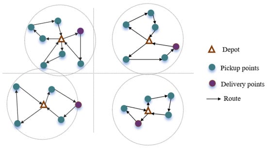
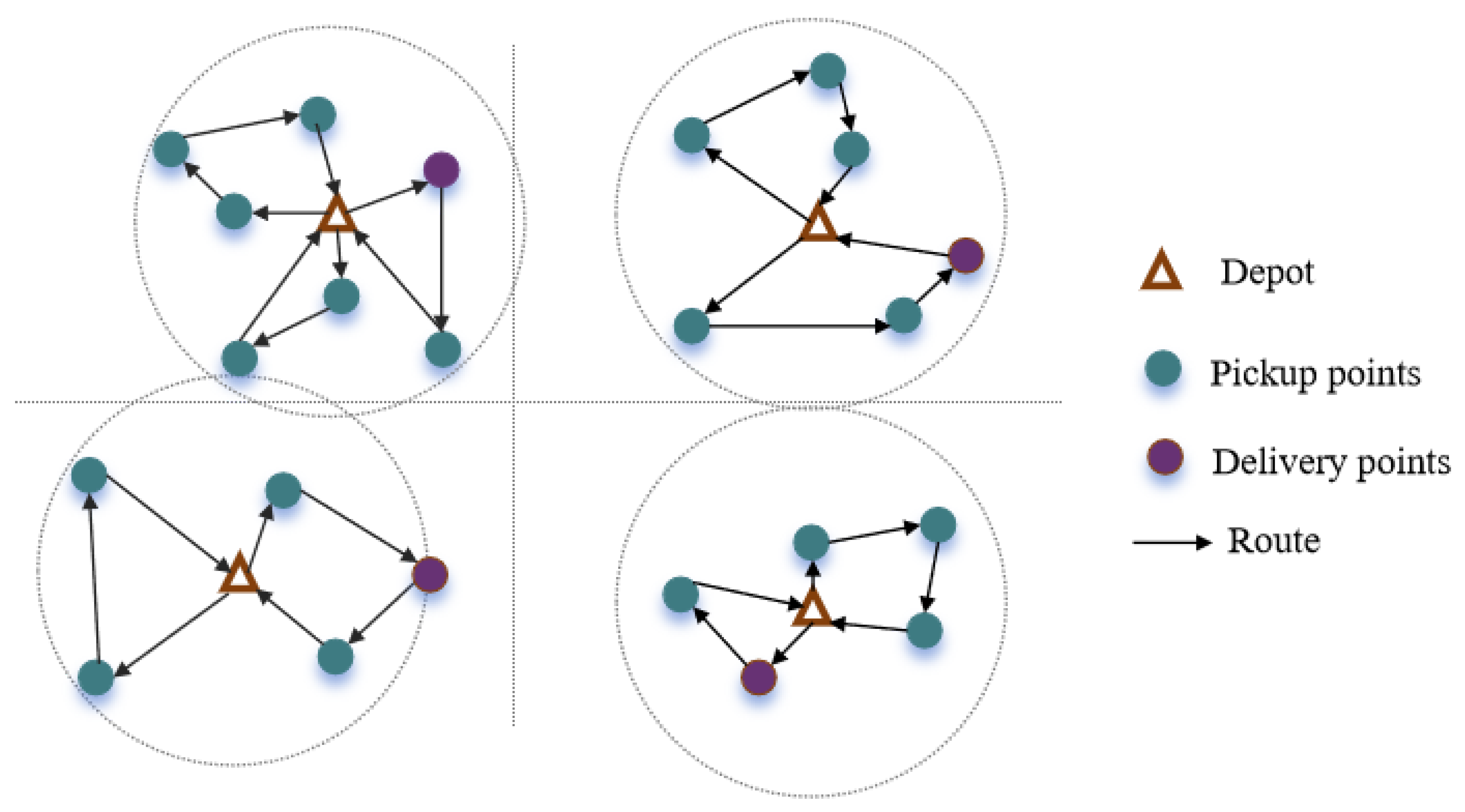
Figure 1 illustrates the energy-aware vehicle routing with pickup–delivery and time windows (EA-VRPPDTW) model. This model employs a multi-depot system and a fleet of vehicles to provide simultaneous delivery and pickup services to a set of customers. The customer set is defined as , the depot set as , and the vehicle set is , where n, m, and k represent the number of customers, depots, and vehicles, respectively.
Figure 1.
EA-VRPPDTW model.
The geographical locations and corresponding time windows for all depots and customers are predetermined. All vehicles are homogeneous, featuring a maximum load capacity Q, and a maximum travel distance which is related to the current vehicle weight . Each customer i () may have either a delivery demand or a pickup demand . The distance between customer i and j is denoted as . The urban road network is time-dependent, meaning vehicle speeds vary with traffic congestion levels across different periods. Each vehicle k, starting from a depot, travels at a time-varying speed (where t denotes the specific time period) and returns to its original depot upon completing its delivery tasks. The travel time between customer i and j is calculated as ; the service time for customer i is set as , which mainly includes unloading and loading times. The model incorporates a fixed vehicle usage cost, alongside variable costs incurred during distribution, such as travel time cost, overtime cost, and service time cost, all of which are based on the total vehicle utilization time. The primary objective of the EA-VRPPDTW model is to assign customers to depots optimally and design vehicle routes that minimize the total integrated cost, encompassing fixed vehicle costs, variable transportation costs, and time window penalty costs.
3.2. Proposed MILP Model for EA-VRPPDTW
EA-VRPPDTW is an NP-hard problem. Constructing a reasonable model for this problem has become a common focus in both academia and industry. This study addresses the EA-VRPPDTW problem by developing a MILP model that incorporates several core constraints, including multiple depots, maximum vehicle capacity, and travel distance corresponding to vehicle load. The primary objective of the constructed MILP model is to appropriately assign all customers to depots and obtain the optimal vehicle routing scheme with minimal total distribution cost for EA-VRPPDTW. The core parameters and decision variables of the model are presented below in Table 1.
Table 1.
Parameters and Variables Used in the Formulation.
3.3. Energy Consumption Model
The energy consumption of an electric vehicle is primarily influenced by its gross weight (including curb weight and payload), road conditions, and its powertrain efficiency. Building upon the fundamental vehicle dynamics model for energy estimation, such as the mechanical power approach adapted from Bektas et al. [28] for conventional trucks, the instantaneous traction power demand (in Watts) for an electric truck can be expressed as a function of the resistance forces encountered during travel, where rolling resistance notably increases with vehicle mass.
where is the total truck mass (kg), g is the gravitational acceleration (), is the truck speed (), a is the acceleration (), is the truck’s frontal area (), is the air density (), and and are the air drag coefficient and rolling resistance coefficient, respectively.
To simplify the analysis, several standard assumptions are adopted. First, the truck is assumed to travel at a constant speed on each road segment, and acceleration effects are neglected (i.e., ). Second, vehicle-related parameters (e.g., aerodynamic drag coefficient and rolling resistance coefficient) are assumed to remain constant across segments, while payload mass and speed may vary by segment. Considering truck k traveling on arc with a horizontal distance of and a constant speed of , the total mass of truck k on arc is:
where represents the payload mass (kg) of truck k on arc . The traction energy (in Joules) required for traversing arc can be derived by integrating the instantaneous power (with ) over the travel time :
Thus, the traction energy consumption simplifies to:
where and are empirical coefficients reflecting vehicle characteristics and environmental parameters. This expression decomposes the traction energy into a speed-related term and a payload-related term, both proportional to travel distance .
For the purpose of this analysis focusing on routing, we assume constant average efficiencies and thus the battery energy consumption is proportional to the traction energy. Therefore, the battery energy consumption (in kWh) for truck k on arc can be expressed as:
where is a constant factor aggregating the drivetrain and battery charge/discharge efficiencies, and the denominator converts Joules to kilowatt-hours (kWh).
Consequently, the total driving energy cost for all vehicles is obtained as follows:
where is the unit price of electricity (RMB/kWh), K is the set of trucks, is the set of arcs, and is a binary variable indicating whether truck k travels on arc .
3.4. Objective Function
3.4.1. Fixed Cost
The fixed cost is incurred when a truck is dispatched from the depot to serve customers and is modeled as:
where P represents the fixed dispatch cost per vehicle.
3.4.2. Time Window Penalty
In logistics distribution processes, delivery timeliness is crucial, as both early and late arrivals can diminish customer satisfaction. In this model, a penalty cost is imposed when vehicles arrive outside customers’ specified time windows [29,30]. The penalty cost is calculated as:
where represents the total time window penalty cost, is the arrival time of vehicle k at customer i, and and are the unit penalty costs for early and late arrivals, respectively.
3.5. Mathematical Model
The complete objective function minimizing the total operational cost is:
Subject to:
The proposed mathematical model incorporates comprehensive constraints to ensure operational feasibility and model correctness. Constraints (10)–(13) govern the fundamental vehicle routing logic, where Constraint (10) ensures each customer is visited exactly once by one vehicle from a depot, Constraint (11) maintains flow conservation between depot departures and customer assignments, Constraint (12) preserves flow balance at each customer node per vehicle, and Constraint (13) guarantees exclusive customer-vehicle assignment. Constraints (14)–(17) manage physical resource limitations, with Constraint (14) enforcing maximum vehicle payload capacity Q, Constraint (15) limiting total energy consumption to , Constraint (16) ensuring arc loads respect capacity and routing decisions, and Constraint (17) maintaining load conservation accounting for both delivery and pickup operations. Constraints (18)–(20) ensure temporal feasibility and route connectivity, where Constraint (18) enforces temporal continuity across customer visits, Constraint (19) eliminates subtours using the MTZ formulation, and Constraint (20) defines bounds for subtour elimination variables. Finally, Constraints (21)–(24) specify variable domains, with Constraints (21) and (22) defining binary routing and assignment variables, and Constraints (23) and (24) specifying non-negativity for load and time variables.
4. A Two-Stage Heuristic for EA-VRPPDTW
To effectively address the EA-VRPPDTW—a complex variant involving multiple depots, time window constraints, and simultaneous pickup and delivery operations-we propose a novel two-stage heuristic methodology(TSH). This approach is designed to systematically decompose and solve the intertwined spatial-temporal and routing decisions inherent in the problem.
The first stage employs a spatio-temporal clustering algorithm that groups customers based on both geographical proximity and temporal compatibility. This is achieved through an integrated distance metric that combines normalized spatial distance with temporal accessibility, ensuring that customers within the same cluster are not only geographically close but also have mutually compatible time windows. The outcome of this stage is an initial assignment of customers to depots, providing a structured foundation for subsequent route construction.
In the second stage, an enhanced Adaptive Large Neighborhood Search (ALNS) algorithm is utilized to generate high-quality vehicle routes. Building upon the initial cluster assignments, this stage introduces several innovative features, including adaptive cross-cluster operation probabilities and specialized destruction–repair operators tailored to the problem’s constraints. The ALNS framework dynamically balances intensification and diversification during the search process, allowing it to explore improvements both within and across cluster boundaries while effectively handling the complex constraints of pickup, delivery, time windows, and energy limits.
By integrating efficient spatio-temporal clustering with a flexible and powerful metaheuristic search, the proposed two-stage heuristic offers a structured yet adaptive solution strategy. It not only enhances computational efficiency through decomposition but also maintains solution quality by enabling inter-cluster optimization in the refinement stage.
4.1. Spatio-Temporal Clustering
Vehicle activities in VRPTW possess both spatial and temporal characteristics. The former refers to the dispersed locations of customers within a specific area, while the latter denotes the time window constraints imposed on services provided to customers. Since vehicle positions and statuses typically change over time, it is reasonable to represent their activities in an integrated manner that considers both spatial and temporal features. This concept is inspired by time geography theory, a methodological framework initially proposed by Hagerstrand [31] and recently employed by numerous researchers in studies of human accessibility and activity patterns [32].
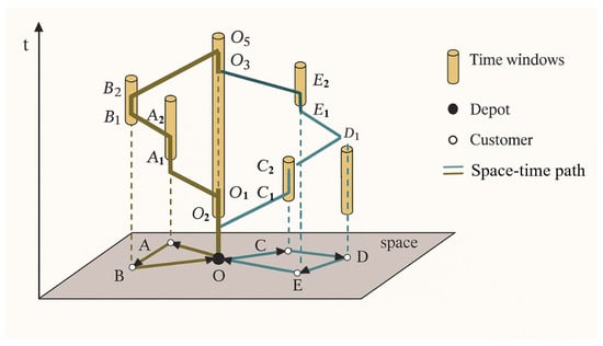
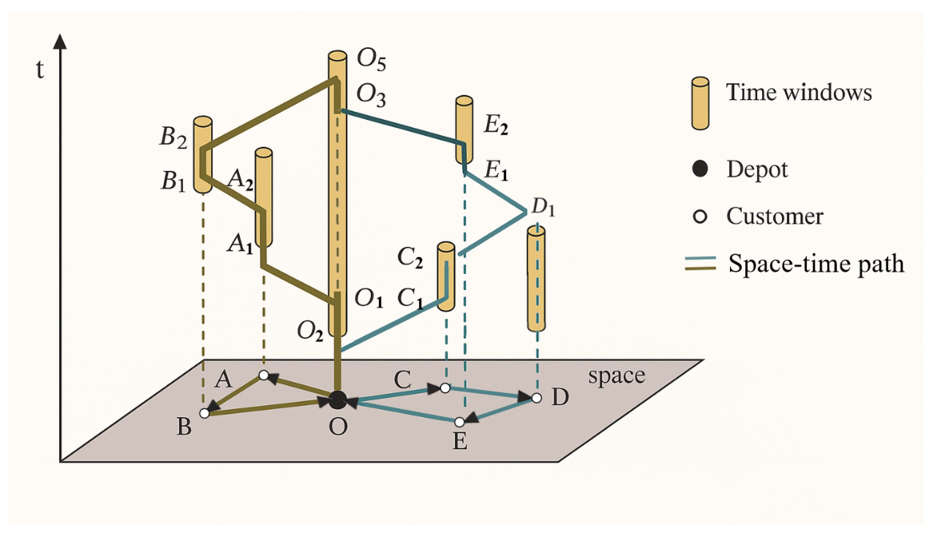
Figure 2 illustrates a VRPTW instance consisting of five customers and two routes: O–A–B and O–C–D–E. The horizontal plane at the bottom represents the two-dimensional spatial layout, while the vertical axis denotes time. Time windows are visualized as cylinders whose heights correspond to the width of the time windows. As can be seen from the figure, when the vehicle follows route O–A–B, it arrives at customer A before its time window opens and therefore incurs an early arrival penalty. In contrast, along route O–C–D–E, the vehicle misses the time window of customer D and thus incurs a late arrival penalty when serving D. The vehicle’s trajectory, O–O1–A1–A2–B1–B2–O3–O5, is referred to as the space–time path. Vertical segments of the space–time path indicate that the vehicle remains stationary during the corresponding time interval, whereas slanted segments reflect the vehicle’s travel speed.
Figure 2.
The space-time path.
4.1.1. Measurement of Spatio-Temporal Distance
To appropriately partition a large number of customers into several clusters, it is necessary to evaluate the distance between each pair of customers. As mentioned earlier, traditional clustering methods only consider spatial distance while ignoring time window constraints. In contrast, our approach incorporates travel time between each customer pair, service time at each stop, and time windows for each customer. It should be noted that routes constructed using VRP methods do not necessarily satisfy time window constraints. However, for any two customers i and j, if a vehicle departs from customer i and arrives at customer j within the predetermined time window, it is preferable for the vehicle to arrive at customer j as early as possible. This approach avoids additional waiting time for the vehicle while facilitating subsequent customer service scheduling. In other words, the remaining time within the time window can be viewed as saved time that can be utilized for arranging the next service. Therefore, it is reasonable to measure temporal distance based on the time saved by vehicles arriving before the time window closes.
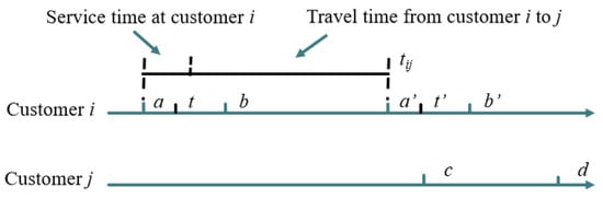
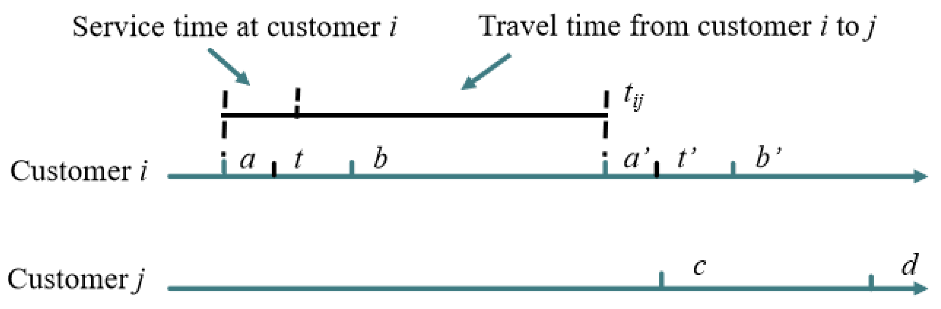
We will provide an example in Figure 3 to discuss in detail how to characterize temporal distance. Consider two customers i and j as shown in Figure 3. Let and represent the time windows of customers i and j, respectively. Let , , and be cost coefficients representing the value of time. Assume the vehicle arrives exactly on time at customer i, meaning the arrival time t falls within time window . The service time at customer i is , and the travel time from customer i to j is . The arrival time at customer j is , where and . Let denote the time saved when the vehicle arrives at customer j at time from customer i.
Figure 3.
Relationship between two customers, considering travel time and service time.
Typically, the specific arrival time at customer j (e.g., ) may occur before, during, or after the time window. Therefore, we can divide the time range into three intervals corresponding to possible arrival times at customer j. can be expressed as a piecewise function corresponding to each interval. The specific division of these three intervals is as follows:
- (i)
- . In this case, the worst scenario occurs when the vehicle arrives at time d, resulting in zero saved time. If the vehicle arrives earlier, the saved time increases linearly at rate until . Here, is suggested to be 1. Then at time c, the optimal saved time is .
- (ii)
- (before the time window’s lower bound). Since early arrival incurs time penalties, we penalize the saved time at rate , where . Note that if the vehicle arrives before (before the time window opens), the saved time will be negative.
- (iii)
- (after the time window’s upper bound). In this case, the vehicle cannot serve the customer within the required time window for the current operation, so a larger penalty should be applied to the saved time at rate , where .
The saved time is defined as follows:
Here, we can observe that represents the temporal accessibility from customer i to j—a larger value indicates easier travel from i to j in the temporal dimension. However, the opposite holds for spatial distance: smaller spatial distance between i and j facilitates easier travel. To harmonize spatial distance with temporal distance and ensure non-negative temporal distance, we define the temporal distance as follows:
Here, A can be set as the maximum time window width among all customers, ensuring non-negative spatio-temporal distances between all customers. Since the arrival time varies from to , we need to evaluate the average condition. Assuming follows a uniform distribution, the expected temporal distance between customers i and j can be represented by integrating over the time window width :
Although the underlying speed function is piecewise, the arrival time is treated as a continuous variable within the interval . Therefore, the expected temporal distance is computed by integrating over this continuous arrival time range under a uniform distribution assumption. This treatment provides a continuous approximation of temporal accessibility, which simplifies the clustering process while preserving the essential effects of time-dependent travel conditions.
4.1.2. Integrated Distance Metric with Regularization
To achieve robust and well-balanced clustering outcomes, we propose an integrated distance metric that synthesizes spatio-temporal proximity with global distribution characteristics. This comprehensive approach incorporates normalized temporal distance, normalized spatial distance, and a novel regularization term designed to enhance clustering stability and quality. The complete distance formulation is expressed as:
In this formulation, represents the normalized temporal distance converted to spatial equivalence, while denotes the normalized spatial distance. Both measures are scaled to the [0,1] range to ensure dimensional consistency and comparability.
The regularization term serves a critical function in our distance metric, where and represent the mean and standard deviation of spatial distances, and and correspond to the mean and standard deviation of temporal distances. This regularization component introduces several important benefits: it enhances robustness against outliers by penalizing distance pairs that deviate significantly from the global distribution; promotes cluster size equilibrium by discouraging the formation of extremely large or small clusters; and incorporates global statistical patterns into local distance calculations, thereby guiding the clustering process toward more globally optimal solutions.
The weighting coefficients , , and control the relative influence of each distance component, satisfying the constraint . This balanced integration ensures that the resulting clusters reflect both geographical proximity and temporal compatibility while maintaining structural coherence through the regularization mechanism.
4.1.3. Constrained Spatio-Temporal Clustering Algorithm
Building upon the integrated distance metric established in the previous section, we present a comprehensive clustering framework and algorithm specifically designed for the EA-VRPPDTW problem. This approach employs a constrained K-medoids methodology that systematically incorporates operational constraints while leveraging spatio-temporal distance measurements to generate feasible and efficient customer clusters.
The clustering framework is structured around three core components (See Algorithm 1): constraint-aware initialization using max-min diversity selection to ensure broad solution space coverage; iterative assignment with multi-constraint feasibility validation; and systematic medoid refinement. This methodological approach addresses the dual challenge of creating operationally viable clusters while maintaining the efficiency benefits of partition-based clustering methods, ensuring that resulting clusters exhibit strong internal cohesion based on both spatial and temporal proximity while maintaining operational feasibility.
| Algorithm 1 Constrained Spatio-Temporal Clustering. |
|
The proposed algorithm significantly extends the standard K-medoids approach through several key enhancements that address the specific requirements of the EA-VRPPDTW problem. It utilizes the comprehensive integrated distance metric that combines normalized temporal distance , normalized spatial distance , and the regularization term to ensure balanced clustering results. The algorithm implements systematic multi-constraint validation that simultaneously verifies capacity constraints, time window compatibility, and energy limitations during customer assignment, ensuring operational feasibility at each step. Furthermore, it incorporates explicit convergence monitoring based on cluster stability rather than relying solely on iteration limits, and maintains constraint-aware medoid updates that preserve feasibility while optimizing cluster cohesion. This comprehensive approach ensures that the resulting clusters are not only geographically and temporally coherent but also operationally feasible, providing a solid foundation for subsequent vehicle routing optimization while addressing the complex constraints inherent in multi-depot vehicle routing problems with simultaneous delivery and pickup.
4.2. ALNS
The ALNS algorithm, developed by Ropke and Pisinger [33] based on the Large Neighborhood Search (LNS) framework introduced by Shaw [34], has gained widespread recognition for its outstanding performance in solving VRP and its variants. The core concept of ALNS involves iteratively destroying and repairing portions of the current solution using a set of diverse operators. The selection of operators is guided by an adaptive, score-based roulette wheel mechanism that dynamically adjusts selection probabilities according to the historical performance of each operator.
Building upon the classical ALNS framework, our proposed approach introduces innovations specifically designed for systematic optimization of clustering-based initial solutions. Algorithm 2 begins by constructing an initial feasible solution where customers are assigned to vehicles according to their cluster allocations. Solution quality is then continuously improved through iterative destruction and repair operations. During the search process, the adaptive mechanism consistently monitors operator performance and dynamically adjusts selection probabilities to favor operators that consistently generate high-quality solutions. The temperature parameter T regulates the acceptance of inferior solutions, promoting exploration in the early stages while gradually shifting focus to exploitation as the search progresses. Notably, we innovatively introduce a dynamic adjustment mechanism for the cross-cluster operation probability , which automatically balances the proportion of cross-cluster and local operations based on their relative performance. This ensures an appropriate equilibrium between intensification and diversification throughout the search process, effectively addressing potential deficiencies in the initial clustering results.
Adaptive Weight Update Mechanism
We innovatively incorporate a cross-cluster probability adjustment mechanism within the adaptive weight update framework. This enhancement specifically addresses the clustering characteristics identified in the first phase of our algorithm, enabling dynamic balancing between intra-cluster optimization and inter-cluster exploration. By automatically adjusting the selection probability of cross-cluster operations based on their demonstrated performance, our method effectively compensates for potential imperfections in the initial clustering results while maintaining the benefits of structured search. This intelligent adaptation mechanism significantly improves the algorithm’s capability to escape local optima and achieve global optimization, thereby enhancing both search efficiency and solution quality.
Roulette Wheel Selection Mechanism: At each iteration, both destruction and repair operators are selected using a roulette wheel method based on their current weights. The selection probability for operator is calculated as:
where k denotes the total number of operators in the same category (destruction or repair). During the initial phase, all operators are assigned equal weights to ensure fair selection opportunities and comprehensive exploration of different search strategies.
Performance Scoring System: Each operator accumulates scores based on its performance during the search process. The scoring criteria are carefully designed to reward operators that contribute to solution improvement while maintaining search diversity. The detailed scoring rules are presented in Table 2.
| Algorithm 2 ALNS for EA-VRPPDTW. |
|
Table 2.
Operator Scoring Rules and Reward Values.
Dynamic Weight Update Rule: The operator weights are updated every iterations (typically 50–100 iterations) based on their recent performance. The weight update formula incorporates both historical performance and recent achievements:
where represents the accumulated score of operator i during the most recent iterations, denotes the usage count of operator i during the same period, and serves as the reaction factor that balances historical performance with recent achievements. Typical values for range between 0.1 and 0.3, ensuring smooth adaptation to changing search conditions.
Cross-Cluster Probability Adjustment: Building upon the clustering characteristics established in the first part of our algorithm, we introduce an innovative cross-cluster probability adjustment mechanism. This feature dynamically balances between intra-cluster optimization and inter-cluster exploration, addressing potential clustering imperfections. The cross-cluster operation probability is adaptively adjusted according to:
where and represent the objective function improvements achieved by cross-cluster and local operations respectively, denotes the total improvement, and is the learning rate parameter. Through this adaptive adjustment, the algorithm automatically increases cross-cluster exploration when it demonstrates superior performance, while favoring local intensification when cross-cluster operations prove less effective. This innovative mechanism ensures optimal balance between exploiting existing cluster structures and exploring potential reassignments across cluster boundaries, effectively addressing the challenge of imperfect initial clustering while maintaining computational efficiency.
5. Computation and Experiments
Currently, there are no standard test instances for the EA-VRPPDTW problem under time-varying speed conditions. In this chapter, we first conduct experiments on multiple small-scale instances to verify the correctness of the model. Subsequently, we select standard instances from both the multi-depot vehicle routing problem and the time-dependent vehicle routing problem to validate the algorithm designed in this chapter. Then, we design test instances for the EA-VRPPDTW problem under time-varying speed conditions to perform experiments on the problem studied. Finally, we conduct a sensitivity analysis of the impact of vehicle speed and load capacity on fuel consumption.
The proposed algorithm for solving the EA-VRPPDTW was implemented in Python 3.9, and all computational experiments were conducted on a machine equipped with an AMD Ryzen 7 6800H 3.20 GHz processor and 16 GB of RAM. Gurobi was employed as the linear programming solver, and a time limit of 7200 s was set for all tests.
5.1. Instance and Parameter Settings
In this study, we evaluate the performance of the proposed algorithm on small-, medium-, and large-scale instances, and analyze the multi-depot time-dependent vehicle routing problem. The weights of the integrated distance metric are set to , , and , consistent with the model specification.
Dataset 1 utilizes data from the standard multi-depot vehicle routing problem instance library (https://neo.lcc.uma.es/vrp/vrp-instances/multiple-depot-vrp-with-time-windows-instances/, accessed on 22 March 2026). This library contains standard test instances for the multi-depot vehicle routing problem with time windows. We selected multiple instances from this library and modified the originally delivery-only demands to include both pickup and delivery demands (each customer has only one type of demand, either pickup or delivery). The allocation of demand types follows a random uniform distribution, ensuring an approximately equal number of pickup and delivery customers in each instance.
Dataset 2 is derived from the Solomon benchmark instance library. To adapt to the multi-depot scenario, we modified the original Solomon instances by expanding a single depot into multiple depots. Specifically, we randomly selected multiple nodes from the original set as depot locations, with the remaining nodes serving as customer nodes. Similarly, each customer’s demand was redefined as either a pickup or delivery demand (each customer has only one type of demand).
Regarding parameter settings, this study follows standard procedures established in existing research. The specific parameter settings are presented in Table 3. In addition, the key parameters of the ALNS algorithm are specified to ensure reproducibility. A simulated annealing acceptance criterion is adopted, with an initial temperature and a geometric cooling rate of , i.e., . The algorithm terminates after a maximum of iterations. For the adaptive operator selection mechanism, the weights of destroy and repair operators are updated every iterations based on their historical performance. Scores are assigned according to the quality of solutions obtained, and operator weights are updated using a reaction factor .
Table 3.
Parameter settings in the case study.
5.2. Computational Results of Experiment 1
To validate the correctness of the proposed model, test instances were designed with customer sizes of 6, 8, 10, and 12 (small-scale) as well as 30, 50, 75, and 100 (medium- and large-scale). Owing to the continuous variation of vehicle speed and the nonlinearity of certain constraints, speed was fixed at 40 km/h throughout the experiments.
All instances were solved with Gurobi under a time limit of 7200 s. It should be noted that, for instances marked with *, the solver does not certify optimality within this time limit. Therefore, the reported MILP results correspond to the best feasible solutions found by Gurobi rather than proven optimal solutions. The “Gap(%)” column reports the percentage deviation of the best heuristic solution from the best solution obtained by Gurobi within the time limit, while “Time(s)” denotes the average computation time. The proposed Two-Stage Heuristic (TSH) is compared against both the MILP solver and a Genetic Algorithm (GA). Each heuristic was run 10 times per instance, recording both the best and the average solution. Performance is evaluated along three dimensions: solution quality, computation time, and algorithm adaptability.
As shown in Table 4, for small-scale instances TSH exhibits excellent performance in both solution quality and computational efficiency. For problems with 6–10 customers, TSH consistently attains the same solutions as the MILP model (Gap = 0.00%), indicating optimal or near-optimal performance, whereas GA yields best-solution deviations ranging from 0.14% to 4.46%. When the instance size increases to 12 customers, the MILP solver can no longer guarantee optimality within the time limit (indicated by *). In this case, TSH still produces solutions that match or slightly improve upon the best solutions found by Gurobi, with gaps between −0.16% and −0.01%. In terms of average solution quality, TSH consistently achieves lower average gaps than GA. This advantage is especially pronounced for the 12-customer cases, where TSH’s average gap (1.58–2.68%) is substantially lower than that of GA (3.43–7.58%), reflecting stronger stability and robustness. Regarding runtime, TSH and GA operate within the same order of magnitude, yet TSH shows better time efficiency as the instance size grows. Overall, for small-scale problems TSH outperforms GA in solution quality, stability, and computational speed.
Table 4.
Comparison between MILP, TSH, and GA in small-scale.
Results for medium- and large-scale instances are presented in Table 5. For medium-scale problems (30 and 50 customers), TSH delivers competitive performance. In the 30-customer group, its best solutions remain very close to the best solutions found by Gurobi within the time limit, with gaps between −0.23% and −0.46%. For 50-customer instances, the best-solution gaps range from −0.71% to −0.95%. Notably, TSH consistently outperforms GA on these medium-scale tests, where GA exhibits positive gaps of 1.10–2.82% for the best solutions. Computationally, TSH completes these instances in 20.25–49.66 s, far below the 7200 s limit imposed on the MILP solver.
Table 5.
Comparison between MILP, TPH, and GA in medium- and large-scale.
For large-scale instances (75 and 100 customers), TSH continues to perform strongly. Best-solution gaps lie between −1.06% and −1.67% for 75 customer cases, and between −1.00% and −1.75% for 100-customer cases, indicating that TSH is able to find solutions better than those obtained by Gurobi within the given time limit. The average gaps for TSH are slightly positive (0.42–3.27%) across all large-scale runs, confirming consistent performance over multiple trials. Runtime scales reasonably with problem size, increasing from about 55–60 s for 75-customer instances to 66–94 s for 100-customer instances-still markedly lower than the time required by an exact MILP approach.
Compared with GA, TSH provides superior solution quality on medium-scale problems while remaining competitive on large-scale ones. GA’s best-solution gaps on large instances range from 2.29% to 4.96%, suggesting less consistent performance in complex settings. Moreover, TSH’s runtimes are comparable to or slightly better than those of GA across all instance sizes.
In summary, TSH exhibits robust performance across the entire spectrum of instance scales. For small problems it achieves optimal or near-optimal solutions rapidly; for medium to large problems it consistently finds high-quality solutions within practical computation times. These results demonstrate that TSH is an effective and efficient approach, particularly when exact methods cannot guarantee optimality within reasonable time limits.
5.3. Computational Results of Experiment 2
The problem studied in this research is the EA-VRPPDTW model with time-dependent speeds, where vehicle speed depends on the time of departure. Following the standard setting in time-dependent VRP literature provided by Figlozzi, the speed is modeled as a piecewise constant function over predefined time intervals. Specifically, the planning horizon T is divided into five periods: , , , , and , within which the speed remains constant but may vary across intervals. The benchmark instances used to validate the proposed TSH algorithm, with four groups of time-dependent speed profiles summarized in Table 6. Given a departure time t from customer i, the travel time is determined by the corresponding speed in the interval containing t. If the trip spans multiple intervals, the travel time is accumulated accordingly across these intervals.
Table 6.
Time-dependent speed functions.
Table 7 presents a comparison of the results obtained by the proposed TPH algorithm and the SA algorithm on standard instances of the time-dependent vehicle routing problem. Here, K denotes the number of trucks required, “Best” indicates the optimal solution found by each algorithm, and “Avg” represents the average of 10 independent runs. As shown in the table, both algorithms consistently yield the same number of trucks () across all four time-dependent speed function groups, indicating that they produce stable and consistent vehicle-scheduling solutions. When comparing solution quality and computational efficiency, the TPH algorithm outperforms SA in terms of both the best solution and the average solution, while also requiring less computation time, demonstrating higher efficiency and stability. These results validate the effectiveness of the TPH algorithm in solving time-dependent vehicle routing problems, confirming that it can maintain high solution quality while significantly reducing computational effort.
Table 7.
Comparison of Experimental Results.
5.4. Sensitivity Analysis
To assess the robustness of the EA-VRPPDTW model and the adaptability of the TSH algorithm to key operational parameters, a comprehensive sensitivity analysis is conducted. This analysis focuses on two dimensions that directly influence routing decisions and total cost: the truck’s energy threshold and the time-dependent travel speed. By systematically varying these parameters, we aim to identify their individual and interactive effects on solution quality (total cost), resource configuration (truck count), and the inherent trade-offs involved.
5.4.1. Energy Threshold Sensitivity Analysis
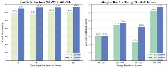
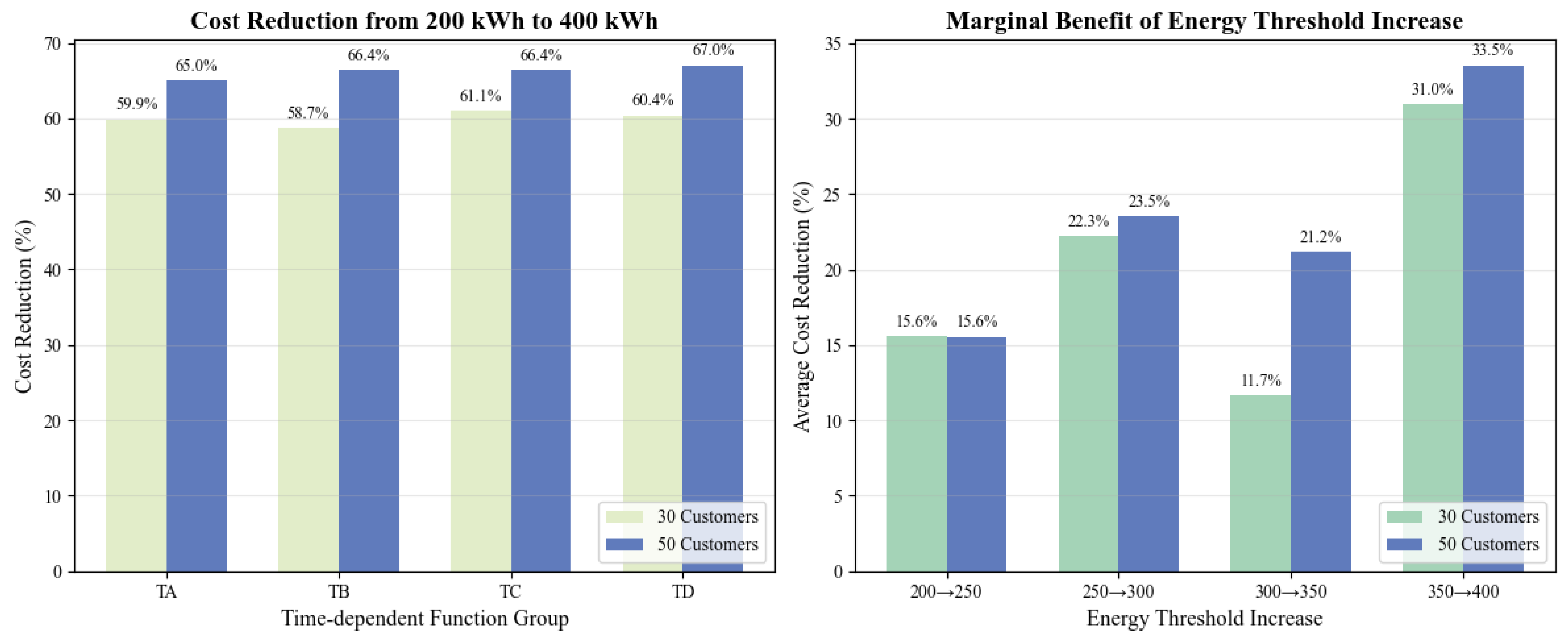
Through sensitivity analysis, it is evident that the energy threshold () exerts a significant and regular influence on both solution quality and vehicle configuration in the time-dependent vehicle routing problem. As the energy threshold increases from 200 kWh to 400 kWh, the total cost shows a clear downward trend (see Figure 4). Taking the RC101_30 instance with the TA1 speed function as an example, the total cost decreases from 1295.03 to 519.67-a reduction of 59.9%-while the number of required vehicles drops from 16 to 5. This simultaneous decline in both cost and vehicle count indicates that enhancing the single-vehicle energy reserve not only directly mitigates route segmentation and additional vehicle dispatches caused by energy constraints, but also improves overall operational efficiency by consolidating delivery tasks and optimizing route structure. In larger-scale instances with 50 customers, this benefit is even more pronounced. Although the absolute cost is higher, the percentage reduction in cost and the proportion of vehicles saved follow a pattern similar to that of smaller instances, demonstrating that raising the energy threshold has a consistently positive impact across different instance sizes under the tested settings.
Figure 4.
Energy threshold sensitivity.
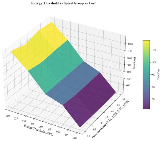
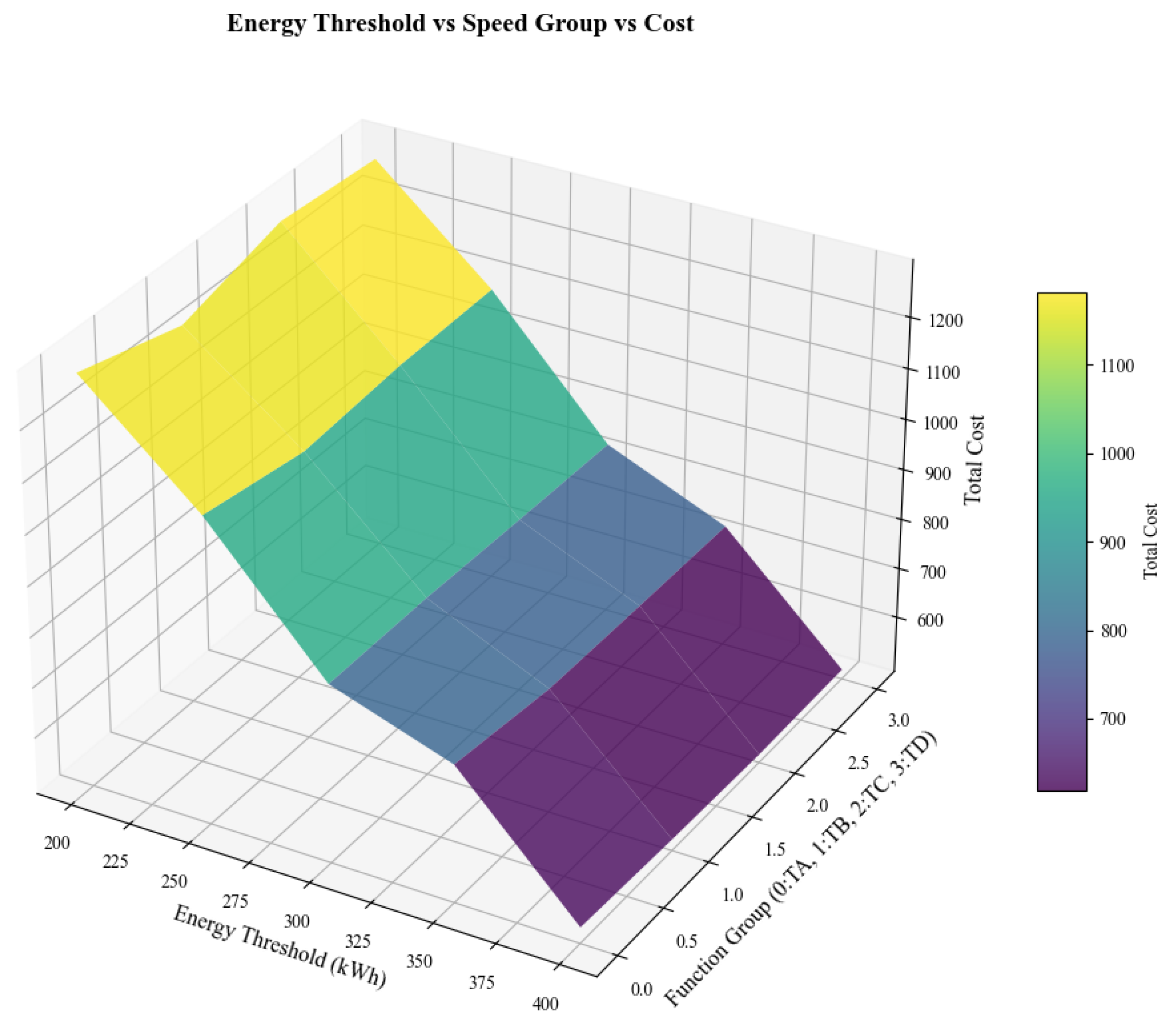
When examining the effect of different time-dependent speed functions, it can be observed that the TB group of functions-especially TB3-generally achieves relatively lower costs under most energy thresholds and instance sizes (see Figure 5). This contrasts with the TA group, which sets higher speed coefficients during multiple periods of the day, leading to increased energy consumption and consequently higher total costs. For instance, in the RC101_30 scenario with kWh, the cost for TB3 is 819.38, whereas for TA3 it is 860.57. This difference reveals that in a time-varying environment, simply pursuing higher speeds does not yield optimal costs; instead, a smoother speed strategy that aligns with the temporal characteristics of the road network is more effective in balancing travel time and energy consumption. The performance of the TC and TD function groups falls between these two, offering alternative speed profile options.
Figure 5.
Energy threshold vs speed group vs. cost.
Notably, under the current test settings, the truck capacity constraint (Q = 1000 kg) is relatively lenient, making the energy threshold the primary bottleneck restricting vehicle configuration and route planning. This is because, in the test instances, customer demand consists mainly of small parcels with low unit weight, causing vehicles to reach their energy limits more readily than their weight limits during actual operations. This observation is supported by the trend that the number of vehicles decreases significantly as the energy threshold increases: when energy constraints are relaxed, vehicles can serve more customers or travel longer distances, whereas the capacity constraint does not trigger a corresponding change in vehicle count. Therefore, in light-parcel delivery scenarios, optimizing energy management holds greater practical value than enhancing load capacity.
5.4.2. Speed Sensitivity Analysis
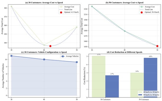
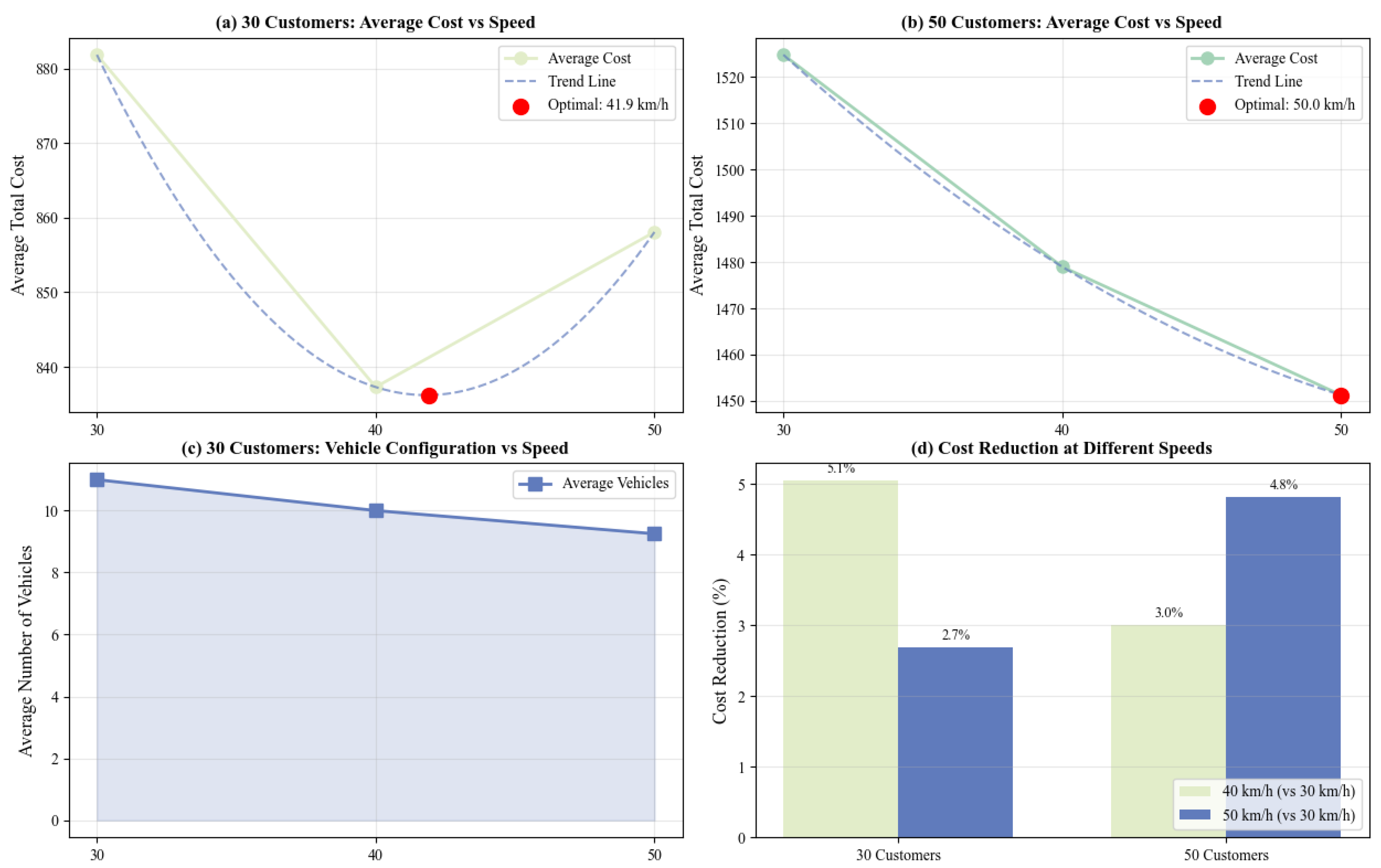
Sensitivity analysis reveals a complex trade-off among vehicle speed, energy consumption cost, and fleet configuration in the time-dependent vehicle routing problem(see Figure 6). When the speed increases from 30 km/h to 40 km/h, although the energy consumption per unit distance rises due to the square-law effect of speed, the reduction in travel time allows each truck to serve more customers or cover a larger area, thereby significantly reducing the number of vehicles required. The resulting savings in fixed costs-including vehicle usage fees and driver wages-often outweigh the increase in energy costs, leading to an overall reduction in total cost. However, when speed is further increased to 50 km/h, the energy cost rises nonlinearly and sharply, and its increment may exceed the fixed-cost savings from further fleet reduction, causing the total cost to rebound in some instances. Meanwhile, although lower speeds (e.g., 30 km/h) help reduce energy consumption, they may extend travel time, increase the risk of time-window violations, and require more vehicles to meet service demands, thereby driving up the total cost. Therefore, route optimization must comprehensively consider the interaction among speed, energy consumption, and vehicle configuration: there exists an economically optimal speed range (approximately 40–45 km/h) in which vehicle resources can be fully utilized, fleet size can be reduced, and energy consumption can be kept at a reasonable level, thereby minimizing total operational costs. This finding provides important guidance for formulating speed strategies in real-world logistics distribution, emphasizing that neither high nor low speeds should be pursued blindly; instead, a balanced point should be identified through systematic optimization.
Figure 6.
Speed sensitivity analysis for time-dependent VRP.
5.4.3. Summary and Implications
The sensitivity analyses on energy threshold and vehicle speed yield consistent and complementary insights. Both confirm that the proposed model effectively captures the critical trade-offs in resource-constrained, time-sensitive routing. The energy threshold analysis highlights its role as a primary constraint in lightweight logistics, where increasing battery capacity can dramatically reduce costs and fleet size. The speed analysis further refines this understanding by identifying an optimal operational speed (40–45 km/h) that balances the conflicting pressures of time savings and energy expenditure. For logistics managers, these findings suggest that, in energy-constrained and light-load delivery scenarios, investing in vehicles with sufficient energy capacity (e.g., around 300–350 kWh for the studied scales) and managing fleet speed toward the identified optimal range can serve as effective levers for cost control. For policymakers and urban planners, the results underscore the importance of considering time-dependent traffic patterns (modeled by the speed functions) in the design of logistics zones and emission regulations.
6. Conclusions
This paper addresses the complex and practical challenge of the energy-aware vehicle routing with pickup–delivery and time windows(EA-VRPPDTW) under multi-depot and time-dependent traffic conditions. To solve this NP-hard problem efficiently, a novel two-stage heuristic (TSH) algorithm is proposed, which systematically integrates spatio-temporal clustering with an enhanced adaptive large neighborhood search (ALNS).
In the first stage, a spatio-temporal clustering mechanism groups customers based on integrated geographical and temporal proximity, providing a structured initial solution that respects both spatial distribution and time window compatibility. The second stage refines these clusters using a tailored ALNS framework, which introduces adaptive cross-cluster operators and specialized destruction–repair mechanisms to effectively explore the solution space beyond initial cluster boundaries.
Extensive computational experiments are conducted using multi-depot benchmark sets and adapted Solomon instances. The results demonstrate that the proposed TSH algorithm outperforms both the exact solver Gurobi (within a time limit) and a genetic algorithm in terms of solution quality, computational efficiency, and stability—particularly in medium- to large-scale instances. Sensitivity analyses further reveal two critical managerial insights. (1) The energy threshold () serves as a primary constraint in lightweight logistics, where increasing battery capacity within an optimal range (300–350 kWh in our tests) can significantly reduce both cost and fleet size, and (2) vehicle speed exhibits a U-shaped relationship with total cost, with an economically optimal speed range around 40–45 km/h that balances travel time savings against energy consumption increases.
The main contributions of this work are threefold. First, we develop a comprehensive mathematical model that integrates time-dependent speeds, battery energy limits, simultaneous pickup and delivery, and multi-depot routing under time windows. Second, we design an efficient two-stage heuristic that decomposes the problem into tractable subproblems without sacrificing solution quality. Third, we provide actionable insights through sensitivity analysis, offering practical guidance for fleet configuration, energy management, and speed control in real-world electric logistics operations.
Future research may extend this work by considering heterogeneous vehicle fleets, dynamic customer requests, integration with charging station scheduling, and application in larger-scale or real-time urban logistics scenarios.
While this study provides a robust deterministic framework, real-world operations are subject to various uncertainties. A critical extension would be to incorporate stochastic disruptions, such as vehicle breakdowns or accidents. Future research could employ a Markov Decision Process (MDP) to model the probabilistic nature of vehicle states and repair times. This would allow for the development of dynamic routing policies that can react to unforeseen delays, thereby enhancing the resilience and practical applicability of the proposed system.
Author Contributions
Conceptualization, Y.W.; Data Curation, Y.W. and J.D.; Investigation, Y.W. and J.D.; Software, Y.W.; Validation, Y.W. and Q.Z.; Writing—Original Draft, Y.W.; Writing—Review and Editing, Y.W. and Q.L.; Methodology, J.D. and Y.D.; Formal Analysis, J.D.; Resources, J.D. and Q.Z.; Funding Acquisition, Y.D. and Q.L.; Supervision, Y.D. and Q.L. All authors have read and agreed to the published version of the manuscript.
Funding
This research received no external funding.
Institutional Review Board Statement
Not applicable.
Informed Consent Statement
Not applicable.
Data Availability Statement
The data presented in this study are available on request from the corresponding author.
Conflicts of Interest
The authors declare no conflicts of interest.
References
- Dantzig, G.B.; Ramser, J.H. The truck dispatching problem. Manag. Sci. 1959, 6, 80–91. [Google Scholar] [CrossRef] [Scilit]
- Lahyani, R.; Khemakhem, M.; Semet, F. Rich vehicle routing problems: From a taxonomy to a definition. Eur. J. Oper. Res. 2015, 241, 1–14. [Google Scholar] [CrossRef] [Scilit]
- Lahyani, R.; Coelho, L.C.; Khemakhem, M.; Laporte, G.; Semet, F. A multi-compartment vehicle routing problem arising in the collection of olive oil in Tunisia. Omega 2015, 51, 1–10. [Google Scholar] [CrossRef] [Scilit]
- Toth, P.; Vigo, D. Vehicle Routing: Problems, Methods, and Applications, 2nd ed.; Society for Industrial and Applied Mathematics: Philadelphia, PA, USA, 2014. [Google Scholar]
- Alinaghian, M.; Shokouhi, N. Multi-depot multi-compartment vehicle routing problem, solved by a hybrid adaptive large neighborhood search. Omega 2018, 76, 85–99. [Google Scholar] [CrossRef] [Scilit]
- Li, Y.B.; Soleimani, H.; Zohal, M. An improved ant colony optimization algorithm for the multi-depot green vehicle routing problem with multiple objectives. J. Clean. Prod. 2019, 227, 1161–1172. [Google Scholar] [CrossRef] [Scilit]
- Gruler, A.; Fikar, C.; Juan, A.A.; Hirsch, P.; Contreras-Bolton, C. Supporting multi-depot and stochastic waste collection management in clustered urban areas via simulation-optimization. J. Simul. 2017, 11, 11–19. [Google Scholar] [CrossRef] [Scilit]
- Wang, Y.; Wei, Z.; Luo, S.; Zhou, J.; Zhen, L. Collaboration and resource sharing in the multidepot time-dependent vehicle routing problem with time windows. Transp. Res. Part E Logist. Transp. 2024, 192, 103798. [Google Scholar] [CrossRef] [Scilit]
- Bouanane, K.; Benadada, Y.; Bencheikh, G. Multi-depots vehicle routing problem with simultaneous delivery and pickup and inventory restrictions: Formulation and resolution. Int. J. Adv. Comput. Sci. Appl. 2019, 10, 110–120. [Google Scholar] [CrossRef] [Scilit]
- Wang, Y.; Gou, M.; Luo, S.; Fan, J.; Wang, H. The multi-depot pickup and delivery vehicle routing problem with time windows and dynamic demands. Eng. Appl. Artif. Intell. 2025, 139, 109700. [Google Scholar] [CrossRef] [Scilit]
- Sadati, M.E.H.; Çatay, B. A hybrid variable neighborhood search approach for the multi-depot green vehicle routing problem. Transp. Res. Part E Logist. Transp. Rev. 2021, 149, 102293. [Google Scholar] [CrossRef] [Scilit]
- Wu, W.; Lin, Y.; Liu, R.; Jin, W. The multi-depot electric vehicle scheduling problem with power grid characteristics. Transp. Res. Part B Methodol. 2022, 155, 322–347. [Google Scholar] [CrossRef] [Scilit]
- Wu, T.Y.; Sun, H. Electric vehicle routing problem with time window and linear weight-related discharging. Control Decis. 2023, 38, 483–491. [Google Scholar]
- Lera-Romero, G.; Bront, J.J.M.; Soulignac, F.J. A branch-cut-and-price algorithm for the time-dependent electric vehicle routing problem with time windows. Eur. J. Oper. Res. 2024, 312, 978–995. [Google Scholar] [CrossRef] [Scilit]
- Kulkarni, R.V.; Bhave, P.R. Integer programming formulations of vehicle routing problems. Eur. J. Oper. Res. 1985, 20, 58–67. [Google Scholar] [CrossRef] [Scilit]
- Shi, Y.; Chen, M.; Qu, T. Vehicle routing problem of an innovative B2C and O2O joint distribution service. Procedia CIRP 2019, 83, 680–683. [Google Scholar] [CrossRef] [Scilit]
- Wang, Y.; Li, Q.; Guan, X.; Fan, J.; Xu, M.; Wang, H. Collaborative multi-depot pickup and delivery vehicle routing problem with split loads and time windows. Knowl.-Based Syst. 2021, 231, 107412. [Google Scholar] [CrossRef] [Scilit]
- Li, J.; Cang, L.; Wu, Y.; Zhang, Z. Two-echelon collaborative many-to-many pickup and delivery problem for agricultural wholesale markets with workload balance. Omega 2025, 130, 103164. [Google Scholar] [CrossRef] [Scilit]
- Zhen, L.; Ma, C.; Wang, K.; Xiao, L.; Zhang, W. Multi-depot multi-trip vehicle routing problem with time windows and release dates. Transp. Res. Part E Logist. Transp. Rev. 2020, 135, 101866. [Google Scholar] [CrossRef] [Scilit]
- Liu, C.; Kou, G.; Zhou, X.; Peng, Y.; Sheng, H.; Alsaadi, F.E. Time-dependent vehicle routing problem with time windows of city logistics with a congestion avoidance approach. Knowl.-Based Syst. 2020, 188, 104813. [Google Scholar] [CrossRef] [Scilit]
- Donati, A.V.; Montemanni, R.; Casagrande, N.; Rizzoli, A.E.; Gambardella, L.M. Time dependent vehicle routing problem with a multi ant colony system. Eur. J. Oper. Res. 2008, 185, 1174–1191. [Google Scholar] [CrossRef] [Scilit]
- Gmira, M.; Gendreau, M.; Lodi, A.; Potvin, J.Y. Tabu search for the time-dependent vehicle routing problem with time windows on a road network. Eur. J. Oper. Res. 2021, 288, 129–140. [Google Scholar] [CrossRef] [Scilit]
- Huang, Y.X.; Zhao, L.; Woensel, T.V.; Gross, J.-P. Time-dependent vehicle routing problem with path flexibility. Transp. Res. Part B Methodol. 2017, 95, 169–195. [Google Scholar] [CrossRef] [Scilit]
- Fan, H.M.; Zhang, Y.G.; Tian, P.J.; Lv, Y.; Fan, H. Time-dependent multi-depot green vehicle routing problem with time windows considering temporal-spatial distance. Comput. Oper. Res. 2021, 129, 105211. [Google Scholar] [CrossRef] [Scilit]
- Pan, B.; Zhang, Z.; Lim, A. Multi-trip time-dependent vehicle routing problem with time windows. Eur. J. Oper. Res. 2021, 291, 218–231. [Google Scholar] [CrossRef] [Scilit]
- Zhao, J.; Gao, Y.; Yang, Z.; Li, J.; Feng, Y.; Qin, Z.; Bai, Z. Truck traffic speed prediction under non-recurrent congestion: Based on optimized deep learning algorithms and GPS data. IEEE Access 2019, 7, 9116–9127. [Google Scholar] [CrossRef] [Scilit]
- Ma, C.; Zhao, Y.; Dai, G.; Xu, X.; Wong, S.C. A novel STFSA-CNN-GRU hybrid model for short-term traffic speed prediction. IEEE Trans. Intell. Transp. Syst. 2022, 24, 3728–3737. [Google Scholar] [CrossRef] [Scilit]
- Bektaş, T.; Laporte, G. The pollution-routing problem. Transp. Res. Part B Methodol. 2011, 45, 1232–1250. [Google Scholar] [CrossRef] [Scilit]
- Chen, C.; Tian, Z.; Yao, B. Optimization of two-stage location–routing–inventory problem with time-windows in food distribution network. Ann. Oper. Res. 2019, 273, 111–134. [Google Scholar]
- Wang, Y.; Duan, J.; Sun, J.; Zhang, Q.; Ye, T. A Green Vehicle Routing Problem with Time-Varying Speeds and Joint Distribution. Sustainability 2025, 17, 7515. [Google Scholar] [CrossRef] [Scilit]
- Hägerstrand, T. What about people in regional science. In Transport Sociology: Social Aspects of Transport Planning; Springer: Berlin/Heidelberg, Germany, 1970; pp. 143–158. [Google Scholar]
- Qi, M.; Lin, W.H.; Li, N.; Miao, X. A spatiotemporal partitioning approach for large-scale vehicle routing problems with time windows. Transp. Res. Part E Logist. Transp. Rev. 2012, 48, 248–257. [Google Scholar] [CrossRef] [Scilit]
- Ropke, S.; Pisinger, D. An adaptive large neighborhood search heuristic for the pickup and delivery problem with time windows. Transp. Sci. 2006, 40, 455–472. [Google Scholar] [CrossRef] [Scilit]
- Shaw, P. Using constraint programming and local search methods to solve vehicle routing problems. In Proceedings of the International Conference on Principles and Practice of Constraint Programming, Pisa, Italy, 26–30 October 1998; Springer: Berlin/Heidelberg, Germany, 1998; pp. 417–431. [Google Scholar]

Disclaimer/Publisher’s Note: The statements, opinions and data contained in all publications are solely those of the individual author(s) and contributor(s) and not of MDPI and/or the editor(s). MDPI and/or the editor(s) disclaim responsibility for any injury to people or property resulting from any ideas, methods, instructions or products referred to in the content. |
© 2026 by the authors. Licensee MDPI, Basel, Switzerland. This article is an open access article distributed under the terms and conditions of the Creative Commons Attribution (CC BY) license.