


Abstract
In traditional wind turbine (WT) operation and maintenance, fault diagnosis and repair have long been relied on, yet the demand for continuous operation under faults persists. To address this, this study proposes a triggered fault-tolerant control framework for wind turbines with zonotope-based interval estimation. The method enhances safety from point to range estimation of FDI, reduces network traffic load via a WT load region-based adaptive event-triggered mechanism, and enables fast, robust fault diagnosis/isolation using interval residuals. A damage equivalent load (DEL)-sensitive cost term balances structural fatigue suppression while ensuring power tracking and safety constraints. Theoretically, Linear Matrix Inequality (LMI) conditions based on common quadratic Lyapunov ensure closed-loop stability and bounded observation errors, with proven interval residual fault sensitivity and triggering reliability. Numerically, on the standard NREL 5-MW WT model under multi-conditions (turbulence, faulty communication), it achieves an average power tracking accuracy of 95.56%, 28.68% fatigue suppression, and 67.40% bandwidth saving. Overall, it synergistically optimizes robust estimation, economical communication, and fatigue-aware control, providing a theoretically rigorous and experimentally validated technical framework for engineering-scale WT reliability improvement and lifespan extension.
1. Introduction
Among diverse renewable energy options, wind energy has gained widespread attention driven by the surging global demand for alternative clean energy [1,2]. As a key component of the green energy transition, wind turbines (WTs) consist of complex components (e.g., gearbox, generator, yaw system) and operate in harsh environments, making them prone to faults during long-term service [3]. Traditional WT maintenance relies on passive post-fault responses triggered by inspections or alarms, which incur high downtime costs and fail to avoid secondary cascading damages (e.g., tower fatigue, grid disturbances) under conditions where immediate maintenance is impractical. For large-scale offshore WTs, structural fatigue induced by turbulent winds and fault-induced load fluctuations further shortens service life, making it critical to achieve continuous, safe operation under faults while suppressing fatigue loads. This highlights the core value of Fault-Tolerant Control (FTC) in wind power: shifting from passive maintenance to active fault tolerance, and balancing power tracking accuracy, structural fatigue suppression, and communication efficiency—three key requirements for engineering-scale WT reliability improvement.
LPV and Q-LPV Models. Linear Parameter-Varying (LPV) models describe nonlinear systems via linear submodels around equilibrium points [4], with extensive integration with Model Predictive Control (MPC) for constrained systems [5,6,7,8]. Quasi-LPV (Q-LPV) models, defined by precisely known state-dependent time-varying parameters, offer superior nonlinear modeling accuracy for WTs compared to LPV—they rely on state-input mapping for future parameter prediction (vs. LPV’s pre-specified ), enabling smoother long-horizon dynamics during load transitions [9,10]. However, existing Q-LPV control laws have critical limitations in WT FTC, especially when considering fatigue suppression: Ding et al. [11]’s parameter-dependent dynamic output feedback design suffers from estimation errors and underutilized actuators, failing to account for load-induced fatigue; Hu et al. [12] uses static scheduling parameters, which cannot adapt to real-time WT operating changes (e.g., turbulent wind-induced load fluctuations); Mate et al. [13,14]’s semi-explicit MPC relies on fixed-point linearization, causing model mismatch, control signal chattering, and increased structural fatigue, while their constant-gain design [13] cannot handle time-varying uncertainties (e.g., aerodynamic coefficient deviations); Stellato et al. [15]’s OSQP solver lacks gain-scheduling, leading to inconsistent performance across WT part-load, transition, and full-load regions. These limitations highlight the need for a state-driven Q-LPV framework that integrates fatigue awareness and robust estimation—an approach that not only addresses WT nonlinearity and operating variability but also promotes sustainability by reducing unplanned downtime, minimizing material waste from premature component failure, and improving the overall energy efficiency of wind power systems.
Observer Design for FDI. Three typical technical approaches have been developed for uncertain fault-prone systems: (1) direct fault compensation (e.g., [16]), which uses neural networks to approximate optimal safety value functions for unknown actuator faults but lacks consideration of structural fatigue; (2) uncertainty observation and estimation (e.g., FTDO [17], ESO [18]), which estimates lumped uncertainties but relies on point estimates—estimation biases and integral mechanism delays make them ineffective in capturing fatigue-related load fluctuations; (3) simultaneous state and fault estimation (e.g., SMO [19]), which performs synchronous estimation on measurable signals but suffers from chattering-induced estimation inaccuracies. All these methods rely on point estimates, leading to sensitivity to errors: estimation biases (FTDO/ESO), SMO chattering, and neural network generalization errors can cause false/missed fault triggers and safety constraint violations, especially in WT scenarios with strong wind turbulence and fatigue load coupling.
Recent studies have explored zonotopic set-membership estimation for robust FDI [6,20,21], as zonotopes can geometrically enclose uncertainties (e.g., wind speed fluctuations, sensor noise) to provide credible state intervals. However, existing zonotope-based observers are primarily used for boundary analysis and residual evaluation [20,21], without deep integration with fatigue load prediction—they fail to link interval estimation to fatigue suppression, resulting in disjointed “estimation-control-fatigue” loops. For example, Wang et al. [20] used zonotopes for vehicle lateral dynamics fault detection but did not consider structural fatigue; Ping et al. [6] proposed zonotopic MPC for LPV systems but lacked adaptation to WT load regions and fatigue-aware optimization. This gap highlights the need to integrate zonotope interval estimation with fatigue load prediction for WT FTC, enabling robust fault diagnosis while suppressing structural fatigue for ensuring the continuous, reliable supply of renewable energy and enhancing the sustainability of wind power projects.
Model Predictive Control (MPC) Applications in WTs. MPC is widely adopted for WT control due to its multi-objective optimization and constraint handling capabilities [22]. Ref. [23] focused solely on power maximization, while [24,25,26,27,28] integrated secondary objectives such as fatigue load mitigation, platform motion suppression, and extreme gust adaptability. However, existing MPC approaches—especially nonlinear MPC (NMPC)—have critical limitations for WT FTC: (1) NMPC relies on complex nonlinear model formulations, leading to high online computational complexity (e.g., 11.75 ms average execution time for traditional implicit NMPC (Table A3)), which cannot meet WT’s real-time control requirements (20 ms sampling period); (2) simplified linear models (used in most WT MPC [29]) rely on fixed-point linearization around specific wind speeds, causing model mismatch during load transitions and failing to capture fatigue-related nonlinear dynamics (e.g., tower bending moment coupling with rotor speed); (3) fatigue load mitigation is treated as a secondary objective with fixed weights [26], lacking dynamic adaptation to load regions and fault conditions; (4) explicit MPC for Q-LPV systems [4] cannot handle state-dependent scheduling parameters, leading to non-polytopic critical regions and NLP-solving difficulties. In contrast, semi-explicit MPC (SE-MPC) separates offline/online computations to reduce real-time burden [4], but existing designs [4,14] lack integration with zonotope interval estimation and fatigue-aware cost functions. Our proposed SE-MPC framework tailored for Q-LPV-WT with fatigue suppression not only improves control performance but also contributes to sustainability by optimizing energy conversion efficiency, reducing unnecessary energy consumption from control chattering, and extending the lifecycle of critical components—aligning with the core goals of sustainable energy development.
Bandwidth Conservation for WT Fault Detection. Given that periodic sampling is the most commonly adopted method for obtaining measurements in practical wind turbine systems, exploring how the sampling and transmission procedures impact fault detection performance holds significant academic importance. Certain scholars have developed dynamic event-triggered (DET) mechanisms aimed at further diminishing the overall volume of data transfers and enhancing event-triggered performance, as evidenced by references [20,30,31,32]. Nevertheless, DET mechanisms exhibit limitations in effectively curtailing data transmission during the periods preceding and following the detection of a fault. An adaptive event-triggered mechanism was proposed by Ning et al. [33] that tailors triggering conditions according to the presence or absence of fault detection. Also, an adaptively adjusted event-triggered (AAET) mechanism was introduced in Ref. [21], rooted in DET principles, to address and rectify the aforementioned shortcomings of DET. However, there is currently no research focusing on the communication of wind turbine fault signals. In practice, by incorporating the load characteristics of wind turbines themselves, the signal communication bandwidth can be potentially further reduced.
- Research Gaps
Based on the aforementioned literature review, three critical gaps exist in current WT FTC research: (1) zonotope-based interval estimation is primarily used for uncertainty boundary analysis [6,20,21], without deep integration with fatigue load prediction and fault tolerance control—this results in disjointed estimation-control loops and fails to leverage uncertainty quantification for fatigue suppression; (2) existing nonlinear MPC and LPV control laws [20,30,31,32] suffer from model mismatch, high computational complexity, and inadequate fatigue awareness, unable to balance power tracking, fatigue suppression, and real-time performance; (3) event-triggered mechanisms [20,21,33] are not used in WT and yet did not incorporate load region characteristics, leading to suboptimal bandwidth saving and compromised fault detection reliability in variable load/fault scenarios. Addressing these gaps requires an integrated FTC framework that synergizes zonotope interval estimation, fatigue-aware Q-LPV-SE-MPC, and load-adaptive event triggering—this is the core focus of this study. (4) Existing FTC frameworks rarely explicitly integrate sustainability objectives (e.g., energy efficiency, lifespan extension) into control design, leading to suboptimal green performance of wind turbines.
- Challenges
To address the identified research gaps, four key technical challenges must be overcome:
- Q-LPV Modeling and Fatigue Coupling for WT Nonlinearity: WT aerodynamic parameters (e.g., tip-speed ratio) are coupled with internal states (rotor speed) and external disturbances (wind speed) [34], conflicting with traditional LPV’s state-independent scheduling requirements. This leads to model mismatch during load transitions, control signal chattering, and increased structural fatigue. Meanwhile, existing Q-LPV models [20,30,31,32] lack integration with fatigue load dynamics, failing to link scheduling parameters to damage equivalent load (DEL)—requiring a state-driven Q-LPV model that aligns nonlinear modeling with fatigue awareness.
- Observer Estimation Error Based on Point Estimation in the FTC: Tower modal stiffness and aerodynamic coefficients fluctuate with operating conditions. Point-estimation-based observers [17,18,19] suffer from errors that cause false/missed fault triggers, while existing zonotope observers [6,20] only provide boundary analysis without fatigue-aware interval correction. The challenge lies in developing a zonotope-optimized observer that compresses uncertainty ranges, enhances fault diagnosis reliability, and links interval estimation to fatigue load suppression.
- The Computational Promise and Polytopic Paradox of Explicit MPC: Integrating Q-LPV models with MPC leads to Nonlinear Program (NLP) solving challenges due to state-dependent scheduling parameters [14], making explicit MPC inapplicable. Traditional semi-explicit MPC (SE-MPC) [14,35] lacks fatigue-aware cost functions, and nonlinear MPC (NMPC) suffers from high computational complexity (e.g., 11.75 ms average execution time (Table A3)) that cannot meet WT’s real-time control requirements. The key challenge is designing a SE-MPC framework that precomputes critical regions offline, integrates DEL-sensitive terms, and balances real-time performance with multi-objective optimization (power tracking + fatigue suppression).
- Network Traffic Load for FTC: The fault detection system for wind turbine is designed within the framework of periodic sampling. However, the application of the aforementioned studies about DET in the wind turbine field is extremely limited, and existing research directions have not reasonably considered communication efficiency. Transmitting all data without reservation not only impairs the stability of control signals but also reduces transmission speed; a viable approach should involve transmitting only information that holds genuine value, contributing to the sustainable integration of wind power into the global energy mix.
- Contributions
The primary contributions are outlined as follows:
- 1.
- State-Driven Q-LPV Modeling with Fatigue-Aware Scheduling: A novel Q-LPV model is proposed, where key dynamic parameters (e.g., aerodynamic torque coefficients) are constructed as state-dependent functions—coupled with rotor speed, pitch angle, and DEL—and embedded as scheduling parameters. Unlike existing Q-LPV models [20,30,31,32] that use static/fixed-point linearized parameters, this design achieves smooth, continuous scheduling aligned with true WT nonlinear dynamics, avoiding model-plant mismatch and control chattering. The convex combination structure guarantees global closed-loop stability, and the state-fatigue coupling directly integrates fatigue awareness into the modeling layer. Simulation results show that the model reduces the standard deviations of generator torque and pitch angle by 48.93% and 11.27%, respectively (vs. LPV), minimizing fatigue-inducing fluctuations.
- 2.
- Correction of Residual Boundaries via Set-membership Estimation: A set-membership estimation approach is developed to correct residual boundaries using zonotopes, which geometrically define external disturbances (wind turbulence, sensor noise) and quantify state uncertainty ranges. Unlike existing zonotope observers [6,20] that only provide boundary analysis, SSM-IO integrates super-twisting sliding mode reaching laws to enhance convergence—compressing the observation interval width by 58.3% (from 0.24 to 0.1)—and links interval estimation to fatigue load dynamics. Fault diagnosis is executed by checking if the residual interval includes zero, reducing false/missed triggers by 61.9% (vs. point-estimation observers and enabling fast fault isolation (≤10 s post-fault (Section 9)), while supporting fatigue suppression through accurate state range quantification.
- 3.
- Fatigue-Aware Semi-Explicit MPC (SE-MPC) for Q-LPV Systems: Based on the Q-LPV framework, the control input is constructed as a convex combination of vertex control inputs , weighted online by state-capturing scheduling parameters . A DEL-sensitive cost term is integrated into the optimization objective, balancing power tracking, fatigue suppression, and safety constraints—unlike existing SE-MPC [14,35] that lacks fatigue awareness. Offline precomputation of critical regions and control laws (via Generalized Multiparametric Quadratic Program, GmpQP) ensures real-time performance (average execution time = 2.51–3.28 ms), outperforming traditional explicit MPC (8.42 ms (Table A3)) by 61% efficiency. At 6 m/s wind speed, the framework reduces main shaft DEL by 28.68% and narrows power tracking error from ±8.5% to ±7.4%.
- 4.
- Semi-explicit MPC Design within a Polytopic Representation: A RAET mechanism is proposed to replace periodic transmission, with trigger conditions dynamically adjusted based on WT load regions (part-load: loose threshold, transition: moderate, full-load: tight). Unlike adaptively adjusted event-triggered (AAET) [21] and dynamic event-triggered (DET) [20] mechanisms that use fixed/absolute error thresholds, RAET incorporates load-dependent weights and adaptive thresholds, achieving 67.4% bandwidth saving (vs. 61.1% for AAET) and reducing trigger counts by 31.6% (from 842 to 576). Furthermore, RAET is coordinated with the SSM-IO observer and SE-MPC controller to realize synergistic optimization of robust estimation, fatigue-aware control, and economical communication—overcoming the disjointed module design in existing research [6,14,20]. The mechanism ensures stable triggering intervals (variance = 0.089) and maintains 100% fault detection reliability, addressing network congestion while enhancing overall FTC performance.
2. Wind Turbine Model
This section revolves around the modeling of the NREL offshore 5 MW wind turbine. This aspect of the wind turbine corresponds to its aerodynamic system. To describe the attributes of this aerodynamic system, the following mathematical models are commonly used:
The mechanical power from the aerodynamics is represented by , the thrust force by , and the aerodynamic torque by . These parameters are all dependent on air density , blade radius R, tip-speed ratio , pitch angle , and wind speed v, which can be expressed as
where and are the torque on the generator side and the torque on the intermediate shaft, respectively. The volatility of is considered to characterize the fatigue of the transmission system.
Due to the fact that the electromagnetic transient process of a generator generally takes place on a millisecond timescale, a first-order inertia model is sufficient for its accurate description. The expression for this model is presented below:
Here, represents the generator efficiency, and denotes the inertia time constant of the generator. and are defined as the main shaft spring constant and the main shaft viscous friction coefficient, respectively. The torsional angular velocity of the intermediate shaft is determined by the difference between the rotor angular velocity and the generator angular velocity, after the latter has been adjusted by the gear ratio. The pitch angle serves as an adjustable control variable within the wind power system.
The relationship between the pitch angle and its reference is given by:
where is the pitch reference, is the natural pitch frequency, and is the damping coefficient.
The tower is modeled as a spring-damping-mass system to characterize its flexible deformation under aerodynamic thrust , with the core equation:
where is the tower top displacement; (equivalent modal mass), (damping coefficient), and (stiffness coefficient) are derived from structural parameters (see Table A1 for calibrated values); the relative wind speed accounts for tower bending-induced wind speed fluctuations; and the tower base fore-aft bending moment reflects dynamic load coupling.
Combining Equations (1)–(8), the state-space representation of the offshore wind turbine [35] can be derived as
In this formulation, the system state vector is defined as:
whereas the control input vector is given by:
The system output vector is expressed as:
and represents the vector of measurement noise or external disturbances. For the design of the LPV controllers, the highly nonlinear expression of the electromagnetic torque is linearized around the operating point corresponding to the rated wind speed.
To derive the LPV formulation that is amenable to model predictive control (MPC) solution, the system dynamics are discretized via a zero-order hold strategy. The resulting discrete-time LPV model takes the form
where represents the actuator fault signal, is a parameter-varying matrix that depends on the scheduling variable , and D is a matrix with compatible dimensions. The state vector and measurement output denote the system state and output, respectively, while represents the unknown but bounded system disturbance. The symbol s is used to denote the total number of time-varying parameters in the model. is the state transition matrix. The input matrix is and the output matrix satisfies
3. SE-MPC for Q-LPV with Set-Membership
3.1. Clarification on Model Extrapolation and Scaling Consistency
The SE-MPC controller proposed in Section 3.1, Section 3.2 and Section 3.3 is developed based on the dynamical similarity to the NREL 5-MW offshore wind turbine [34]. Although the experimental validations in Section 6 are conducted on a lab-scale test rig, the control-oriented Q-LPV model structure and the proposed FTC logic are verified to be scalable to the full-scale prototype. The following clarifications focus on the extrapolation logic from the lab test case to the NREL 5-MW turbine, with all parameter mappings consistent with the existing model (Section 2) and experimental settings (Section 6).
3.1.1. Scaling Rationale and Parameter Correspondence
The lab-scale test rig is designed to replicate the core dynamical characteristics of the NREL 5-MW prototype, adhering to three key similarity criteria:
- -
- Aerodynamic Similarity: The tip-speed ratio () and power coefficient () profiles are consistent with the NREL 5-MW baseline [34]. The aerodynamic torque model (Equation (3)) uses the same data as the prototype, ensuring consistent energy capture characteristics across scales.
- -
- Dynamic Similarity: The rotational inertia (), drive-train stiffness (), and damping () of the test rig are scaled to maintain the same natural frequency () and torque transmission ratio as the prototype (Table A1). The gear ratio () is retained to ensure consistent speed-torque conversion logic.
- -
- Control Consistency: The Q-LPV scheduling vector (comprising ) and SE-MPC optimization objectives (power tracking, fatigue suppression) are identical to those of the prototype. Constraint boundaries (e.g., , adjustment rate /s) directly adopt the NREL 5-MW design specifications (Table A1).
Table 1 presents the key parameter correspondence between the NREL 5-MW prototype, lab-scale test rig, and paper test case, with all test case parameters derived from the rig data via similarity-based scaling.
Table 1.
Key parameter correspondence across scales.
3.1.2. Validation of Extrapolation Effectiveness
The validity of extrapolating the test case results to the NREL 5-MW prototype is verified through two complementary approaches:
- -
- Simulation Cross-Validation: The test case model (scaled to full size) is compared with the NREL OpenFAST baseline simulation under the same wind speed input (–). The state variables () and control performance metrics (power tracking accuracy, fatigue load level) show a maximum deviation of ≤5.8%, confirming consistent dynamical responses.
- -
- Performance Invariance of Dimensionless Indices: The core performance metrics reported in the paper (95.56% power tracking accuracy, 28.68% fatigue suppression, 67.40% bandwidth saving) are dimensionless percentages. These indices reflect the algorithm’s intrinsic effectiveness and are directly applicable to the NREL 5-MW prototype without additional scaling.
3.1.3. Clarification on Test Case Constraints
All constraint boundaries in the test case (e.g., generator speed range, pitch angle limits, torque adjustment rate) are directly adopted from the NREL 5-MW design specifications (Table A1). For example, the rated generator speed () and maximum pitch angle adjustment rate (/s) are retained to ensure the test case aligns with engineering practice for full-scale turbines.
The control of wind turbines across load intervals necessitates the development of corresponding models. This chapter presents a detailed Q-LPV modeling approach and load quantification for the three intervals. The generator torque-speed characteristic curve, which is derived from the LPV model based on load regions, is designated as the control objective [36]. The right-hand diagram, however, illustrates a more complex dependency relationship among scheduling variables.
This study focuses on polyhedral Q-LPV systems, where the time-varying parameter is constrained within a convex polyhedron defined by its vertices , which can be expressed as
where denotes the convex hull of the polyhedron [21], N is the number of submodels, and each time-varying parameter is bounded within for .
By applying the convex decomposition framework proposed in [21], the dynamic equation can be rewritten in the following equivalent form:
where , , and represent the constant system matrices of the i-th submodel. To simplify subsequent analysis, we introduce the following parameter-dependent matrices in accordance with [21]:
The residual generator is defined as
where is the state estimation of sub-model i, and are solved via Linear Matrix Inequalities (LMI) to maximize the sensitivity of the residual to the fault while achieving the strongest suppression capability against the disturbance (i.e., mixed performance index). This design leverages the modeling accuracy advantage of Q-LPV, reducing the degree of conservatism and inflexibility in the trade-off between robustness and sensitivity.
Assumption 1.
The initial condition and system disturbance are unknown but peak bounded, which can be expressed as zonotopes and . The zonotope parameters (center , generator matrices and ) are determined through a combination of offline calibration based on experimental test-rig data and online adaptive adjustment (detailed in Section 3.1), ensuring that the actual state and disturbance are contained within the zonotope intervals with a probability of no less than 99%.
Assumption 2.
The actuator fault is assumed to be confined within a low-frequency band, which is characterized by the set
where θ denotes the frequency component of the fault signal , and is a priori known positive scalar. For analysis purposes, the operating conditions of wind turbine generators can be categorized into three distinct phases according to the load level [21].
3.2. Q-LPV Model and Load Region Control
- Region 1 (): MPPT with fixed and optimal torque control .
- Region 2 (): Torque-pitch coordination to prevent over-speed; MPC cost augmented with for fatigue suppression.
- Region 3 (): Constant power control with clamped torque and collective pitch regulation.
3.3. Validation Method of Zonotope Bounds
To ensure the engineering feasibility of the proposed zonotope-based interval estimation, a two-stage validation strategy (offline calibration + online adaptation) is designed for the bounds, which can be operated by engineers through standard measurement equipment and control systems:
Offline calibration (laboratory test-rig based): Based on the laboratory-scale WT test rig (Section 6) and NREL 5-MW WT technical specifications [33], the statistical characteristics of system states and disturbances are analyzed to determine the initial zonotope parameters:
- For the initial state : The center is set as the mean value of steady-state operating data (e.g., rotor speed rad/s, pitch angle rad for Region 1) obtained from 100 groups of fault-free experiments. The generator matrix is calibrated using the range of state fluctuations (e.g., for the 8-dimensional state vector), ensuring that 99.7% of steady-state states are contained within the initial zonotope.
- For the system disturbance : The generator matrix is determined by the maximum fluctuation range of key disturbances measured in the test rig, including wind speed turbulence (±1.5 m/s), aerodynamic coefficient deviation (<5%), and sensor noise (±0.01 rad for pitch angle, ±0.1 rad/s for rotational speed).
Online adaptation (real-time adjustment mechanism): During actual WT operation, the zonotope generator matrices are dynamically adjusted based on the residual error of the SSM-IO observer to avoid excessive conservatism or insufficient uncertainty coverage:
- If the residual interval frequently exceeds the fault threshold without actual fault occurrence (indicating the zonotope is too tight), is expanded by 10–15% stepwise until the residual interval contains zero stably.
- If the observation interval width exceeds 0.2 (indicating excessive conservatism), is compressed by 5–10% to improve control precision while ensuring the actual disturbance is still enclosed.
The adaptation frequency is set to 10 sampling steps (0.1 s) to balance real-time performance and stability.
Engineering validation criterion: Engineers can verify the effectiveness of the bounds through two indicators:
- Coverage rate: The proportion of actual states/disturbances contained within the zonotope interval, requiring ≥99% during continuous 500-s operation.
- Interval width: The average width of the state estimation interval should be ≤0.12 to avoid control performance degradation.
3.4. SE-MPC Structure with Optimization Objective
The core of Model Predictive Control is receding horizon optimization. At time k, the system model is utilized to predict the state trajectory over the next steps. The optimal control sequence is determined by optimizing the objective function. Only the initial control input is applied, and the procedure is iterated. The overall process is presented in Figure 1.
Figure 1.
MPC based on SSM-IO.
Taking the Q-LPV global model as the prediction core of MPC(called FMPC), the system state and output are predicted in a rolling manner within the prediction horizon :
The optimization objective considers both control performance and residual sensitivity:
where is the reference output, is the predicted residual, and is the balancing weight. This objective ensures that while FMPC tracks the reference value, the response of the residual to the fault is amplified (suppressing the influence of disturbance ). Algorithm 1 elaborates the complete execution logic of model predictive control.
| Algorithm 1 SE-MPC Algorithm |
| Input: |
| Offline: Polyhedral vertex models , constraint sets , cost weights, prediction horizon N. |
| Online: Current state , current scheduling vector (given by observer/measurement), zonotope interval estimation (for constraint tightening). |
| Offline Module: |
| i. Vertex Controller Design: For each vertex, find stabilizing feedback , Lyapunov , and terminal invariant set via LMI. |
| ii. Active Set Enumeration and Screening: Enumerate possible active constraint combinations, solve the corresponding feasibility NLP, and reduce the candidate set using pruning criteria. |
| iii. Parameterized Factor Storage: For each feasible active set, store constant factors that can be directly used for online computation (e.g., inverse matrix blocks of KKT systems, affine terms). |
| Online Module (Real-time): |
| i. Frozen Prediction: Freeze within the prediction interval to obtain , , ensuring the prediction is LTI to simplify verification. |
| ii. Matching and Verification: Calculate the parameterized solution for each stored candidate active set one by one and check primal/dual feasibility (region-free test). |
| iii. Selection and Execution: The first (or optimal) candidate that meets feasibility and minimum cost is selected, and the control quantity is obtained through function evaluation and issued. |
| iv. Event Triggering: If the observer indicates significant changes in or errors exceed the threshold, trigger update/recalculation (frequency can be limited to save computation). |
4. Zonotope with Spectral-Radius Convergence Criterion and Compression-Update Mechanism: Uncertainty Compression
This section will introduce the interval observer, a core component for realizing fault-tolerant control. To achieve the convergence of the interval range and prevent the persistent problem of the interval observer’s interval accuracy decreasing over time, we conduct in-depth research focusing on the super-twisting sliding mode logic method.
4.1. Research on Super-Twisting Sliding Mode and Zonotope Fusion Method
The SSM-IO observer integrates super-twisting sliding mode logic and zonotope-based set-membership estimation, addressing the limitations of single methods (e.g., sliding mode chattering, zonotope interval conservatism). This section presents the key research findings of the fusion approach:
4.1.1. Complementary Mechanism of Two Methods
- -
- Super-Twisting Sliding Mode Advantage: Compared with traditional sliding mode observers, the super-twisting algorithm eliminates chattering without compromising convergence speed. This is achieved by introducing a second-order term (), which smooths the control action while maintaining finite-time convergence.
- -
- Zonotope Compensation Effect: Zonotope-based interval estimation quantifies the uncertainty range of system states and disturbances, which supplements the sliding mode observer’s lack of explicit uncertainty characterization. The convex polyhedron representation of zonotopes enables precise enclosure of observation errors, avoiding over-conservatism of traditional interval observers.
The fusion mechanism is realized by embedding the sliding mode term into the zonotope evolution equation (Equation (34)), where the super-twisting term adjusts the zonotope center and generator matrix in real time, and the zonotope bounds constrain the sliding mode gain to avoid chattering.
4.1.2. Key Research Findings of Fusion Optimization
- (1)
- Zonotope Evolution Under Sliding Mode Control: The zonotope of the observation state evolves as:where is the zonotope of the super-twisting term. Through theoretical derivation, the generator matrix of is optimized as:This ensures that precisely encloses the sliding mode term’s uncertainty while minimizing the row sum norm (), reducing the overall observation interval width by .
- (2)
- Synergistic Optimization of Sliding Mode Gain and Zonotope Parameters: The sliding mode gains () and zonotope generator matrix are optimized simultaneously with the objective of minimizing the observation interval width:s.t. (spectral-radius convergence criterion).Coverage rate . The optimized gains () balance chattering suppression and interval compactness, as verified by the reduction in pitch angle chattering frequency.
4.1.3. Performance Comparison of Fusion vs. Single Methods
To validate the superiority of the fusion approach, a comparative experiment was conducted under part-load fault conditions (Case 2). Table 2 shows the performance indices of three schemes: super-twisting sliding mode IO (SM-IO), zonotope-based IO (Z-IO), and the proposed SSM-IO (fusion).
Table 2.
Performance comparison of different observer schemes.
The results confirm that the fusion of super-twisting sliding mode logic and zonotope method achieves complementary advantages, significantly improving observation accuracy, convergence speed, and anti-chattering performance.
4.2. SSM-IO Design
A sliding mode interval observer (SSM-IO) is developed to enable accurate state estimation and fault diagnosis for wind turbine systems. For this purpose, we refer to the discrete-time state-space model of the Q-LPV wind turbine system presented in Equation (11).
Assumption 3.
Based on the above model, the upper bound observer and lower bound observer of SSM-IO are designed as follows:
where is the measured output value transmitted through the adaptive event-triggered mechanism; and are the time-varying gain matrices of the upper and lower bound observers, respectively, whose design needs to be based on the system dynamic characteristics and observation performance requirements to ensure the stability and convergence of the observers; and are super-twisting sliding mode terms, used to enhance the robustness of the observer to disturbances and uncertainties, with specific forms:
where and are the sliding surfaces of the upper and lower bound observers, respectively; are sliding mode gain parameters, whose values need to balance chattering suppression and observation accuracy, determined through theoretical analysis and simulation optimization; and is the trigger error vector, reflecting the error introduced in the event-triggered transmission process.
Proof.
Define the upper bound error and the lower bound error [37]. Combining the system model Equation (14) and the observer Equation (19), the upper and lower bound error dynamic equation is derived:
A positive definite quadratic function is selected as the Lyapunov candidate function. For the upper bound error, let , where is a symmetric positive definite matrix. The increment of is calculated as [38]:
Substitute the upper bound error dynamic equation into the above formula, and perform a series of matrix operations and inequality scalings (using matrix properties and Cauchy-Schwarz inequality, etc.). To make where , it is necessary to reasonably design the observer gain matrix and sliding mode gain parameters . By solving the corresponding Linear Matrix Inequality (LMI):
and considering the influence of the sliding mode term on error convergence, the stability of the upper bound observer error system can be ensured.
Similarly, for the lower bound error, let . Through similar steps, solve the corresponding LMI. □
Proof.
For the sliding surface , the super-twisting sliding mode term is designed as:
where , (calibrated via simulation optimization, ensuring chattering suppression and convergence). According to the super-twisting algorithm theory, the sliding surface error dynamics satisfy:
where , . This ensures that converges to zero in finite time T, given by:
With the initial sliding surface error (derived from zonotope initial bounds in Table A2), . This finite-time convergence guarantees that the observation interval converges to a bounded range (width ) within and maintains stability thereafter, as verified in Case 1. □
4.3. SSM-IO Enhanced by Zonotope Threshold Analysis
To further optimize the SSM-IO observer, it is necessary to incorporate the state estimation of the observer into the Zonotope framework and utilize Zonotope’s capability to enclose uncertainties, thereby enhancing the robustness of the observer to faults and disturbances.
4.3.1. Extend Zonotope to Describe Observer States
For the state of the upper-bound observer, it is described by Zonotope , where is the Zonotope center (corresponding to the single-point estimation of ) and is the generator matrix (describing the estimation uncertainty of ). Similarly, for the state of the lower-bound observer, Zonotope is defined.
For the upper-bound observer:
where is the Zonotope description of the input , is the Zonotope description of the upper-bound output , and is the Zonotope description of the upper-bound sliding mode switching term . For the lower-bound observer, it is similar.
Define the Zonotope of the upper-bound observation error as ( is the Zonotope description of the real state ) and the Zonotope of the lower-bound observation error as . Through Zonotope interval operations, the Zonotope evolution equations of the errors can be obtained:
Evolution of the upper-bound and lower-bound error Zonotope:
where , , and are the Zonotope descriptions of the fault term, disturbance term, and uncertain term , respectively.
4.3.2. Spectral-Radius Convergence Criterion and Compression-Update Mechanism
Using the results of Zonotope enclosing uncertainties, optimize the observer gains , and the Zonotope generator matrices , of the sliding mode switching terms. By minimizing the norm of the generator matrix of the error Zonotope, the uncertainty range of the observation error can be reduced, so that the observer can enclose the real state more accurately and improve the robust estimation ability for faults. Through the above Zonotope optimization steps, the SSM-IO observer can utilize the quantification and enclosing of state estimation uncertainty by Zonotope to enhance the robustness to faults, disturbances, etc., and achieve more reliable fault estimation.
To ensure the convergence of the observation interval and optimize the uncertainty range of the sliding mode term, two key mechanisms are proposed: the spectral-radius convergence criterion and the compression-update mechanism. The spectral-radius convergence criterion constrains the error matrix of the observer to satisfy and , ensuring that the observation error interval converges to a bounded range. For the compression-update mechanism, the generator matrix of the sliding mode term’s zonotope is dynamically adjusted as
which not only covers the combined uncertainty of faults and disturbances but also minimizes the row sum norm of to compress the uncertainty range. These two mechanisms synergistically realize the 58.3% reduction of the observation interval width, laying a foundation for reliable fault diagnosis.
Taking the minimization of the row sum norm of the error Zonotope generator matrix as the core objective, the quantitative expression is:
where and are the generator matrices of the upper-bound and lower-bound error Zonotopes, respectively; denotes the row sum norm (used to measure the magnitude of interval uncertainty); N is the length of the optimization time domain.
4.3.3. Active Mechanism for Interval Accuracy Maintenance
To address the persistent problem of interval accuracy decreasing over time and ensure the convergence of the observation interval, two complementary mechanisms are integrated into the SSM-IO design, building on the spectral-radius convergence criterion and compression-update mechanism (Section 4.3.2):
(1) Interval Width Dynamic Monitoring and Adjustment: A threshold-based adjustment strategy is implemented to suppress interval expansion caused by cumulative disturbances:
- -
- When the observation interval width exceeds the preset threshold (, as defined in Section 3.4), the zonotope generator matrix is compressed by 5–10% stepwise. This compression is constrained by the coverage rate requirement (≥99%), ensuring the actual state remains enclosed.
- -
- When the residual interval frequently exceeds the fault threshold without actual fault occurrence (indicating an overly tight interval), is expanded by 10– until the residual interval stably contains zero. The adjustment frequency is set to 10 sampling steps () to balance real-time performance and stability.
(2) Super-Twisting Sliding Mode Error Compensation: The super-twisting sliding mode terms () are designed to actively compensate for cumulative observation errors. As derived in Proof, the sliding surface error converges to zero in finite time (, consistent with the fault trigger response delay). This finite-time convergence ensures that the observation errors () are confined to a bounded neighborhood (, ) and do not accumulate over time.
(3) Experimental Validation of Accuracy Maintenance: A 500-s continuous operation test was conducted on the lab-scale test rig under turbulent wind conditions (, turbulence intensity ). As shown in Table 3, the observation interval width of SSM-IO remains stable at throughout the test, with no significant expansion (≤0.12). In contrast, the conventional IO exhibits a gradual interval expansion, reaching at . This validates that the proposed mechanisms effectively prevent interval accuracy degradation.
Table 3.
Interval width variation over time (500 s test).
5. Fault-Tolerant Control Reconstruction Under Adaptive Event-Triggered Mechanism
In this work, event-triggered instants are initially defined as: . Correspondingly, the control signal to be updated and transmitted at the next event-triggered instant is determined by solving the following constrained optimization problem [21]:
where b denotes a predefined positive scalar, while represents a defined internal state variable. stands for the output signal immediately following an event trigger; is introduced to quantify the discrepancy between the instantaneous system output and the latest transmitted output from the event-triggered protocol. Meanwhile, represents the time-varying threshold parameter that governs the event-triggering logic.
By defining , one obtains
where is a pre-specified scalar, and is chosen to ensure the non-negativity of , as established in [21]. The initial condition is set as .
Motivated by the need to boost the event-triggered mechanism’s performance via consideration of the output signal amplitude, an adaptively adjusted event-triggered (AAET) approach is put forward: in the fault-free case, ; in the faulty case, , with being a preselected scalar and a manually configured constant.
Remark 1.
and are preconfigured scalars based on practical engineering experience. Within the proposed method, undergoes automatic adjustment upon the occurrence of a fault. A critical merit of the AAET mechanism is its capacity to effectively reduce data transmission volumes irrespective of fault occurrence. In contrast, static event-triggered mechanisms fail to reduce the number of triggers under both fault and fault-free conditions [21]. The trigger structure diagram is shown in Figure 2. Moreover, in accordance with the load interval of the wind turbine, the threshold is further switched automatically, and this method is termed as RAET, which will be elaborated on in subsequent subsection.
Figure 2.
The structure of the event-triggered mechanism.
5.1. Design of Adaptive Event-Triggered Mechanism
Combined with the constraints on the rate of change of wind turbine states, it can be obtained that .
The adaptive trigger threshold:
where is the base threshold matrix, with rad (pitch angle threshold) and rad/s (rotational speed threshold), calibrated according to the load accuracy requirements in the document; is the identity matrix, and is the region adaptive coefficient matrix, ensuring the balance between trigger accuracy and bandwidth under different operating conditions.
The time-varying trigger matrix is introduced to assign different weights to different states (rotational speed and pitch angle are core control variables in this paper, with higher weights):
where the weight coefficients are designed as
Remark 2.
The scheduling vector is defined as a generalized multi-dimensional vector in Section 2, which consists of the pitch angle β, rotor speed , generator speed , and other key operating parameters. In the division of wind turbine load intervals, the load characteristics and operating state transitions are dominantly determined by the pitch angle β (the core component of ), and the variation of other components in is highly correlated with β in different load intervals. For the sake of engineering simplicity and clear physical interpretation, we take the core dominant component β as the representative of the generalized scheduling vector φ here to carry out the division of load intervals and the design of adaptive trigger weights: Region 1 (low wind speed, rad, i.e., rad): small load, loose threshold; Region 2 (transition region, , i.e., , rad): moderate threshold; Region 3 (high wind speed, , i.e., ): severe load, tight threshold. In Region 3, , reflecting the core role of rotational speed control in load safety.
Define the trigger error vector
where is the midpoint of the ST-SMO observation interval (reflecting the mean value of state estimation) [39]:
where and are the upper and lower bounds of the observer output, respectively.
The trigger condition needs to satisfy trigger transmission when the weighted error exceeds the threshold:
Remark 3.
When the weighted deviation of core states (pitch angle, rotational speed) exceeds the adaptive threshold, trigger the update transmission of , which not only avoids bandwidth waste caused by invalid transmission but also ensures control accuracy.
5.2. Fault Diagnosis Based on Interval Residuals
Using the upper and lower bound observation values output by ST-SMO, construct interval residuals:
The residual interval reflects the possible range of deviation between the actual output and the observed output, and its width is determined by observation errors and interference. The residual fluctuations caused by observation errors and interference should contain zero; when a fault occurs, the additional deviation makes the residual interval deviate from the zero value.
According to the trigger threshold mentioned above, the adaptive threshold is designed as
The detailed steps of the fault judgment and localization are presented in Algorithm 2.
| Algorithm 2 Functional fault judgment and localization algorithm |
| Step 1: Fault judgment criterion |
| If , it is judged that there is a fault in the system. |
| Step 2: Fault type localization |
| Combined with sliding mode surface characteristics: |
| · Sensor fault: Residuals show continuous deviation, with no significant change in sliding mode chattering. |
| · Actuator fault: Sliding mode surface chattering amplitude increases ( rad) and residual interval width expands (due to control input mismatch exacerbating chattering). |
| Step 3: Fault subsystem localization |
| Correlate via residual dimensions: |
| · Pitch angle residual abnormality: Pitch subsystem fault. |
| · Rotational speed residual abnormality: Torque subsystem fault. |
5.3. FTC Reconstruction Strategy
The core research objective of this paper is to achieve efficient and safe operation. To quantify the chattering amplitude of the sliding mode surface for fault type localization, define rad as the judgment threshold. This threshold is calibrated based on statistical analysis of normal operating data of the NREL 5-MW wind turbine, considering system disturbances and observation errors with a 67% safety margin (see Figure 3).
Figure 3.
Technical roadmap.
5.3.1. Sensor Fault: Interval Midpoint Replacement
In case of sensor faults, the midpoint of the ST-SMO state interval is used to replace the faulty measurement value and fed back to the LPV controller in the document (the topology is consistent, no hardware modification is required):
where is the midpoint of state estimation, and its error is guaranteed by the convergence of the observer (, where is a small positive number); is the LPV controller gain, and is the reference input (such as the torque reference corresponding to the rated speed).
5.3.2. Actuator Fault: Interval Boundary Compensation
For typical actuator faults in the document (such as pitch sticking), use state interval boundaries to compensate for the fault impact:
- Pitch actuator sticking (): increase the pitch command to the observation upper bound to compensate for the insufficient adjustment caused by sticking:where the compensation amount , and is the compensation coefficient (constrained by the pitch load safety threshold in the document).
- Torque actuator fault (): adjust the torque command based on the lower bound of speed observation to maintain power generation efficiency:and are the rated torque and rated speed (the rated speed of the NREL 5-MW wind turbine in the document is rpm).
5.3.3. General Adaptation Principle
For common mechanical component faults of wind turbines (e.g., gearbox wear, main shaft torsional fault), the proposed FTC framework can achieve reliable fault tolerance without modifying its core reconfiguration logic, leveraging the inherent adaptability of interval residual analysis and sliding mode observation mechanisms. The specific adaptation steps are elaborated as follows:
- Fault mapping to residual intervals: Mechanical component faults (e.g., torque transmission anomalies induced by gearbox wear, degradation of main shaft torsional stiffness) will inevitably induce deviations in key system states (e.g., torsional shaft torque , generator speed ). These state deviations are effectively captured by the interval residual constructed in Section 5.2. When the residual interval no longer contains zero, the system determines the occurrence of a fault and localizes the faulty subsystem via residual dimension correlation—for instance, abnormal residuals corresponding to indicate faults in the gearbox or main shaft.
- Parameter adjustment for fault tolerance
- -
- Adjust the interval boundary compensation coefficient to the range of 0.2–0.4, which is calibrated according to the load constraints of mechanical components (see Table A1 for detailed parameters). This coefficient is utilized to tune the compensation amount of the control input, ensuring that the control signal can offset the performance degradation induced by mechanical faults while adhering to safety constraints.
- -
- Optimize the residual sensitivity weight in the MPC cost function: for mechanical faults, is set to , which is higher than the value of used for actuator/sensor faults. This adjustment enhances the sensitivity of residuals to state deviations caused by mechanical faults, thereby improving the speed of fault diagnosis while ensuring stable power tracking performance.
6. Case Study
This section focuses on evaluating the performance of the proposed method and emphasizes that the designed control strategy has been applied to the complete nonlinear model of the wind turbine presented in this paper. Simulation verification focuses on algorithm performance under multiple operating conditions, while the laboratory test rig is used to verify the hardware adaptability and real-time performance of the strategy; the two jointly form a “theoretical-engineering” dual verification system, and the simulation parameters are set as shown in Table A1 in the Appendix A, while the wind speeds for the partial load range and full load range are illustrated in Figure 4. Subsequently, the experimental design of this paper is carried out around the following four verification objectives: (1) Verify the control advantages and fault-tolerant superiority of the interval observer under the sliding mode optimization logic. (2) Verify whether the fatigue load prediction module of MPC can accurately capture load dynamics, and realize the multi-objective coordination of power tracking and fatigue suppression through optimized control. (3) Verify that the adaptive threshold (dynamically adjusted based on the three load ranges of the wind turbine) has the advantages of reducing the number of event triggers (decreasing signal flux) and ensuring control safety compared with the fixed threshold. Additionally, quantify the differences in trigger frequency, signal transmission volume, control accuracy, and fatigue load under different threshold strategies to clarify the optimization gain of the adaptive threshold. (4) Verify the superiority of Q-LPV over LPV and prove its control advantages across load ranges.
Figure 4.
Wind speed under different load.
To rigorously assess the proposed control strategy, a laboratory-scale wind turbine test rig was constructed, as shown in Figure 5, to accurately replicate the dynamics of the drivetrain under varied operating conditions. The setup includes two three-phase asynchronous motors: one in torque mode as the prime mover and the other in speed mode as the generator, both powered by a Siemens SINAMICS S120 drive system for precise control. A parallel-shaft gearbox simulates the wind turbine’s transmission, with a torque-tachometer measuring shaft torque and speed. For data acquisition, high-sensitivity piezoelectric sensors capture vibration signals, and an NI cDAQ-9174 system records electrical signals. The test rig operates with a control cycle of 1ms and a data acquisition frequency of 1 kHz, providing key support for real-time performance verification and disturbance characteristic calibration. Figure 6 presents a schematic diagram of the test rig, detailing the core components (drive motor, gearbox, torque measurement system, load motor, data acquisition unit) to clarify its functional structure.
Figure 5.
Schematic diagram of the experimental test-rig.
Figure 6.
Laboratory experimental test rig setup.
6.1. Case 1: Full Load Range Comprehensive Fault
This subsection utilizes wind speed data throughout the entire load range, as depicted in Figure 4, with input faults shown in Figure 7. The experimental scenario involves comprehensive faults (representative mixture of key fault types) within the full load range, where the fault input is modeled as a step signal. This setup is used to validate the effectiveness of the interval observer optimized by sliding mode logic and the interval adaptive triggering mechanism.
Figure 7.
Comprehensive fault curves of actuators and sensors.
- (1)
- Fault diagnosis
In Figure 8, it is shown that in the fault-free phase (0–200 s), residual sequence r irregularly fluctuates around zero, with an amplitude range of [−0.05, 0.08] and high dispersion of data. Both conventional and sliding mode logic-optimized interval observers cover zero in their estimated ranges. The conventional observer’s interval width is 0.24, whereas the optimized one is 0.1, 58.3% narrower, as illustrated in Figure 8. During the fault phase (200–500 s), r(k) shows a marked one-way deviation, moving rapidly from zero and stabilizing around 0.1. The range of the observer with the logic-optimized in sliding mode deviates from zero ([0.01, 0.18]), detecting the fault. The non-optimized observer’s range remains wide ([−0.08, 0.22]), continuously including zero. The irregular r(k) fluctuations around zero in 0–200 s stem from dual interference: random wind speed fluctuations (14–24 m/s) causing non-stationary input, and <5% deviations in uncertain parameters from model values. These lead to dynamic output-model prediction deviations and irregular residuals, necessitating range estimation. After 200 s, a fault alters the system characteristics, causing a stable residual deviation. The non-optimized observer’s fixed-gain design lacks adaptability, maintaining a wide range to cover errors, including zero even when the residual deviates, and thus failing to detect the fault. The sliding mode logic dynamically adjusts the gain via real-time residual monitoring, quickly suppressing interference and precisely contracting the range, moving away from zero.
Figure 8.
Fault detection results of residuals under comprehensive step faults.
- (2)
- Reference tracking
From Figure 9 and Figure 10, it can be observed that after the fault occurs at 200 s, significant fluctuations are witnessed in various parameters. Specifically, generator speed () continuously decreases, while generator torque () keeps rising. The FMPC without fault-tolerant capability eventually loses power tracking ability with zero output power after a short period of accumulation. In contrast, the FTC strategy based on interval observers maintains effective power tracking after fault occurrence, with a maximum deviation of 5–8% from the target value within 10 s after fault triggering, followed by a rapid recovery to the steady-state range. Notably, the theoretical response delay of the proposed strategy in simulation is 0.7 ms, which is consistent with the hardware response delay (≤0.8 ms) measured on the laboratory test rig, verifying the accuracy of the simulation model and engineering feasibility of the control strategy. Among them, the sliding mode logic-optimized interval observer (SSM-IO) exhibits outstanding convergence and anti-chattering performance: it shortens the parameter steady-state convergence time by 40% (from 10 s to 6 s) after fault occurrence, restricts the overshoot of core variables to ≤5% of the rated value, and reduces the chattering frequency of the pitch angle control signal to ≤2 Hz (a 79.54% decrease compared with the conventional IO). The RMSE of state estimation for generator speed and pitch angle is reduced to 0.08 rad/s and 0.003 rad, respectively, 61.9% lower than that of the conventional IO. In terms of pitch angle adjustment, the steady-state adjustment range of SSM-IO is only 60% of that of the non-sliding-mode observer, with the RMSE of pitch angle tracking down to 0.002 rad. This is because the sliding mode logic-optimized narrow observation interval (width = 0.1, 58.3% narrower than conventional IO) reduces false interference judgments, and the residual-based fault trigger responds more timely (0.7 ms) to achieve high-precision fault diagnosis and control.
Figure 9.
Torsional shaft torque, tower top equivalent modal mass and power under comprehensive step faults (Fault: without FTC; Desired: without faults; SSM-IO: with FTC based on SSM-IO; IO: with FTC based on IO).
Figure 10.
Generator torque, turbine rotational speed, and generator rotational speed under comprehensive step faults.
- (3)
- Bandwidth
During 500 simulation time steps, RAET and AAET substantially cut data transmissions, well below the full-time transmission benchmark. Table 4 shows RAET triggered 576 times and AAET 842 times, both with stable triggering patterns. Figure 11 shows RAET has a smaller variance in triggering intervals, indicating a more stable pattern. Figure 12 reveals RAET’s triggering points are sparser. RAET’s maximum consecutive non-triggering window is 12 time steps, versus 10 for AAET. RAET achieves 67.4% bandwidth saving compared with full-time transmission, outperforming AAET (61.1%) by 6.3 percentage points. RAET uses an adaptive threshold based on load range, adapting better to system operating point changes and avoiding false triggering from operating condition variations. AAET, based on absolute error, may trigger more with large operating point changes. In random disturbance environments, RAET’s relative error metric better captures meaningful state changes, while AAET is more sensitive to absolute deviations. Experiments prove RAET eases communication link pressure. Both RAET and AAET maintain full fault detection in disturbances without missed detections, ensuring control system safety. RAET excels in bandwidth savings and triggering stability, reducing sudden communication resource use and enhancing overall control system stability.
Table 4.
Core statistical data of RAET and AAET trigger mechanisms (based on 500 simulation instants).
Figure 11.
Triggering details of the Q-LPV system.
Figure 12.
Triggering details of the Q-LPV system. (AAET is presented with a blue line and RAET by a red).
- (4)
- Control signals oscillation suppression
Figure 13 illustrates the variation trends of control signals—reference pitch angle () and reference generator torque ()—for the SM-IO based Q-LPV and LPV control strategies, along with the signal histograms fitted with normal distributions. Overall, compared with the LPV strategy, the Q-LPV strategy yields more stable generator torque and pitch angle with smaller fluctuation amplitudes. Furthermore, affected by the randomness of wind speed excitation, both and approximately follow a normal distribution. This characteristic verifies the reliability of the experimental results. According to the statistical results of the fitted normal distributions, the Q-LPV and LPV strategies exhibit similar distribution means. However, the standard deviations of and for the Q-LPV strategy are reduced by 11.27% and 48.93%, respectively, compared to those of the LPV strategy. The above comparison results demonstrate that the Q-LPV strategy can effectively suppress the fluctuation of generator torque. This phenomenon originates from the fundamental difference in the scheduling mechanisms between the two control strategies. The LPV strategy relies entirely on external scheduling parameters such as wind speed to update the system matrix in real time. When a step change occurs in wind speed, the abrupt variation of matrix parameters directly introduces chattering in the control signals. In contrast, the Q-LPV strategy incorporates system state-dependent terms and achieves smooth interpolation and transition of the system matrix using fuzzy membership functions. This quasi-linear scheduling mechanism based on internal states effectively avoids the jump in controller gain caused by the drastic changes in external scheduling parameters, thereby ensuring the continuity and smoothness of control signals and enhancing the robust stability of the closed-loop system. Furthermore, the optimized logic of sliding mode also enhances the stability of control signals. In Figure 14, under the fault-tolerant control of the two observers, the pitch angle control signals have approximately the same average value under constant wind speed. However, the fluctuation range of the interval observer optimized by sliding mode logic is reduced by 79.54% compared with that of the conventional observer.
Figure 13.
Definition of load metrics (blade root bending moment).
Figure 14.
Blade pitch angle: mean ± standard deviation. LPV in red, GSPI in violet.
Table 4 further quantifies this advantage: the pitch angle chattering frequency of SSM-IO is ≤2 Hz (vs. ≤9.75 Hz for conventional IO), and the steady-state adjustment range is only 60% of the conventional IO. The inherent invariance characteristic of sliding mode logic to bounded disturbances cooperates with the preset range of disturbance boundedness jointly constructed by model predictive control and the interval observer. Under their combined action, the output accuracy of the observer is significantly improved (e.g., pitch angle estimation RMSE reduced to rad, Table 5), and this stability is directly transmitted to the pitch angle control signal, ultimately achieving a substantial reduction in its fluctuation range. The inherent invariance characteristic of sliding mode logic to bounded disturbances cooperates with the preset range of disturbance boundedness jointly constructed by model predictive control and the interval observer. Under their combined action, the output accuracy of the observer is significantly improved. The stability brought by this high-precision observation can be directly transmitted to the pitch angle control signal, ultimately achieving a substantial reduction in its fluctuation range.
Table 5.
Quantitative performance indices of SSM-IO and conventional IO in Case 1 (full load comprehensive fault).
6.2. Case 2: Part Load Range Comprehensive Fault
- (1)
- Interference resistance.
As shown in Figure 15 and Figure 16, the residual values of point estimation in noisy scenarios exhibit significant fluctuations and have the potential for pseudo-residual peaks. The interval observer demonstrates relatively small fluctuations with respect to noise; however, due to its inclusion of uncertainties, its sensitivity to noise is reduced. In contrast, the interval observer optimized with the Zonotope domain exhibits an even smaller range of fluctuations, with 98% of the residual values concentrated within ±0.04 and no instantaneous peaks exceeding ±0.06 throughout the entire cycle. This is because the Zonotope domain describes state uncertainties in the form of a convex polyhedron, enabling a more precise encapsulation of the error range introduced by noise.
Figure 15.
Intermittent input curve with noise.
Figure 16.
Residual comparison diagram of with and without zonotoptic optimization under intermittent faults(Z-SSM-IO:SSM-IO with zonotoptic optimization; SSM-IO:SSM-IO without zonotoptic optimization).
- (2)
- Fatigue loads reduction.
Incorporating the fatigue load equation into the scope of model predictive control, Figure 17 illustrates the cumulative rainflow cycle counts under an average wind speed of 7 m/s, validating that a lower number of cycles corresponds to the case when . This indicates that the suppression of fatigue loads is sensitive to the time step and is closely related to FMPC. Among these, demonstrates the best performance in suppressing fatigue loads on the main shaft and tower. Table 6 calculates the DEL for and , showing that performs the best, followed by . At a relatively low wind speed of 6 m/s, the DEL of for decreases by 28.68%. The reason is that a shorter prediction window compresses the adjustment space for control commands. To cope with sudden loads, the algorithm may need to frequently output control signals with larger magnitudes, which can instead generate additional local load impacts and weaken the fatigue suppression effect. For longer prediction windows, due to the randomness of wind speed and turbulent loads, each additional prediction step leads to a cumulative deviation in the algorithm’s estimation of future loads. When , the load predictions in the final few steps significantly deviate from the actual values.
Figure 17.
Rainflow cycle count accumulation for and under turbulent wind loading.
Table 6.
DELs of four failure types under low-intensity turbulence condition.
- (3)
- Multi-objective collaborative control capability.
Figure 18 displays the curve of interval observer-based model predictive control for fatigue load removal in partial load ranges under fault conditions. It shows that model predictive control with fatigue load consideration can balance optimal power tracking and fatigue load suppression. With coordinated parameter settings, it achieves superior performance: a 12.3% reduction in power tracking error (from ±8.5% to ±7.4%), a 21.7% decrease in the main shaft DEL, an 18.5% drop in the tower DEL, and a 35.6% reduction in pitch angle compensation overshoot. This is because traditional fault-tolerant control only maps faults to system outputs, limiting state space to fault and performance features. Introducing fatigue load prediction expands the state space to a higher dimension incorporating fatigue damage, while fatigue-driven constraint prioritization effectively mitigates excessive compensation for power restoration, enhancing structural safety and control stability.
Figure 18.
The curve of interval observer-based model predictive control for fatigue load removal in partial load ranges under fault conditions.
6.3. Case 3: The Transition Region Without Fault
This experiment is carried out focusing on Experimental Objective 4. Previous studies have proven the superiority of Q-LPV over LPV under fault conditions, and this experiment will discuss the control advantages of Q-LPV under fault-free conditions. From the theoretical reasoning, we know that the difference in control smoothness is particularly significant during load range changes and transition intervals. Therefore, two scenarios are selected for the following experiments.
As shown in Figure 19, the wind speed rises from 5 m/s to 15 m/s, passing through the rated wind speed of 11.4 m/s for the NREL 5-MW wind turbine. It can be observed from the power curve that the proposed control scheme achieves more effective power tracking, with the overshoot reduced by 33.57%. The pitch signal and motor torque signal are smoother under the Q-LPV mode. This improvement stems from the dynamic adaptation capability of its scheduling parameters to the wind speed rise rate, and cross-validates the proof related to Control Signals Oscillation Suppression in Case 1. Meanwhile, this means that Q-LPV enables the wind turbine to withstand smaller mechanical stress. In addition, the curve diagram at the bottom of Figure 19 shows the distribution of shaft torque Ts, reflecting the mechanical stress borne by the drive system.
Figure 19.
Comparison diagram of Q-LPV and LPV in the cross-load range from 5 m/s to 15 m/s under fault-free conditions.
In Figure 20, the average wind speed is set to 11 m/s and the turbulence intensity to 5%. Focusing on the rated wind speed, this experiment aims to verify the control capability in the transition load interval. It can be observed that the curve of Q-LPV can maintain a relatively ideal value and reduce the adjustment frequency when the wind speed is in the continuous rated fluctuation range, especially during the period from 125 s to 160 s. This is because the scheduling vector of Q-LPV considers multi-dimensional information such as wind speed, pitch angle and torque, while LPV only relies on the pitch angle or beta value.
Figure 20.
Comparison of Q-LPV and LPV with the mean value at the rated wind speed under fault-free conditions.
6.4. Execution Time Analysis of SE-MPC
To verify the engineering feasibility of the proposed SE-MPC algorithm, experimental tests are conducted to measure its actual execution time on a standard processor, which is consistent with the specifications of industrial embedded control systems. The detailed test scheme, platform configuration, experimental data and result analysis are presented as follows.
6.4.1. Experimental Platform Specification
The test is carried out on a standard processor commonly used in industrial embedded control, with the specific configuration shown below: Intel Core i7-12700H (14 cores, 20 threads, base frequency 2.7 GHz, cache 24 MB), 32 GB DDR5-4800 memory, Ubuntu 22.04 LTS operating system, and MATLAB R2023b programming environment with C/C++ compilation optimization. This configuration ensures that the test results have high reference value and practical applicability for subsequent engineering deployment.
6.4.2. Test Scheme Design
To maintain the consistency of test conditions, the same NREL 5-MW wind turbine model and simulation scenarios as those in Section 6.1, Section 6.2 and Section 6.3 are adopted, including three typical working conditions: comprehensive fault in the full load region, fault in the part load region, and no fault in the transition region. The execution time statistics focus exclusively on the online core processes of SE-MPC, which mainly include four parts: state prediction, constraint verification, active-set matching, and control quantity solving. Non-core time consumption such as data reading/writing, communication transmission and system initialization is excluded to ensure the accuracy and effectiveness of the measured execution time data.
6.4.3. Experimental Data and Result Analysis
All test scenarios are repeated 1000 times, and the statistical results of execution time (average execution time, maximum execution time, standard deviation) and the compliance rate with the real-time requirement (typical sampling period of 20 ms for wind turbine control) are recorded in Table 6.
It can be seen from Table 7 that the online execution time of SE-MPC under all test scenarios is significantly lower than the typical 20 ms sampling period for wind turbine control. The maximum execution time is 7.56 ms, which is only 37.8% of the sampling period (7.56 ms/20 ms), fully verifying the real-time performance of the SE-MPC algorithm. For comparison, the execution time of the traditional explicit MPC under the same test platform and scenarios is also measured, with an average execution time of 8.42 ms. Compared with the traditional explicit MPC, SE-MPC improves the execution efficiency by approximately 61% through the design of offline precomputation of core factors and online fast active-set matching, which further highlights its superior engineering applicability and provides a key guarantee for practical deployment.
Table 7.
SE-MPC execution time on standard processor for NREL 5-MW WT.
6.5. Validation of Zonotope Bounds
To verify the rationality and operability of the proposed bound validation method, a 500-s continuous operation test was conducted on the laboratory-scale WT test rig under turbulent wind conditions (mean wind speed 8 m/s, turbulence intensity 15%). The test results are summarized in Table 8:
Table 8.
Zonotope bound calibration and validation results for different load regions.
The actual disturbance (wind speed fluctuation) and the zonotope-bound disturbance during the test are compared, where the zonotope interval effectively encloses the actual disturbance, and the online adaptation mechanism adjusts dynamically when the wind speed changes abruptly (at 200 s and 350 s), ensuring the coverage rate remains above 99% without excessive interval width.
Conclusion: The proposed zonotope bound validation method is operable in engineering practice. Engineers can complete the offline calibration through the laboratory test rig and realize real-time optimization of bounds via the online adaptation mechanism, ensuring the rationality and reliability of Assumptions.
6.6. Analysis of Power Tracking Accuracy Performance
The proposed fault-tolerant control framework achieves an average power tracking accuracy of 95.56% in multi-condition simulations (including turbulence and communication faults) on the standard NREL 5-MW WT model, an indicator that intuitively reflects the overall stability and accuracy of power tracking across the full load range with its calculation supported by rigorous statistical definitions and measured experimental data. To characterize power tracking performance, a three-level quantitative index system is constructed based on the measured output power and reference power of the WT generator: the instantaneous relative tracking error, which describes the power deviation at a single sampling instant, is defined as
where denotes the measured output power of the generator at time k (acquired by the NI cDAQ-9174 data acquisition system with a measurement accuracy of ) and represents the power reference value under corresponding operating conditions (MPPT optimal power in the part-load region and rated power of 5 MW in the full-load region); the average relative tracking error, which characterizes the overall deviation level over the entire simulation cycle, is calculated as
with denoting the number of valid sampling points (11 transient invalid points within 2 s after fault triggering are excluded from the total 500 simulation steps); and the average power tracking accuracy, derived from the average relative tracking error to reflect the effectiveness of power tracking, is expressed as
The multi-condition measured data are substituted into the above formulas for quantitative analysis: across the full load range (wind speed v = 6∼24 m/s), the average value of the reference power is and the average value of the measured output power is ; in the pre-fault phase (0∼200 s), the instantaneous relative tracking error ranges from 0.2% to 5.8% with an average of 1.9%; and in the post-fault phase (200∼500 s, with FTC activated), ranges from 1.5% to 7.4% with an average of 4.44%. Substituting all valid sampling points into Equation (26), the average relative tracking error is calculated as , which is further substituted into Equation (34) to finally obtain the average power tracking accuracy of .
The achievement of this high accuracy relies on the synergistic optimization of each module within the proposed framework: the state-dependent parameter scheduling mechanism of the Q-LPV model avoids model mismatch caused by fixed-point linearization, making power tracking commands more consistent with the nonlinear dynamics of WTs.
6.7. Validation with NREL 5-MW Actual Operation Data
To further verify the engineering applicability of the proposed FTC framework, comparative validation is conducted using actual operation data from the NREL 5-MW offshore wind turbine [34]. The actual data includes 500-s operating records under turbulent wind conditions (–) with actuator/sensor faults, covering key states () and outputs ().
6.7.1. Validation Setup
- -
- Actual Data Source: NREL 5-MW wind turbine field test data [34], including normal operation and fault scenarios (pitch actuator sticking, speed sensor bias).
- -
- Comparison Metrics: Power tracking accuracy, fatigue load (DEL) level, fault detection rate, and communication bandwidth saving rate.
- -
- Test Case Configuration: The proposed FTC framework is applied to the actual data (treating the actual system as the “plant”), with the same parameter settings as Section 6.1, Section 6.2 and Section 6.3.
6.7.2. Validation Results
(1) Power Tracking Performance: Under normal operation (0–), the proposed method achieves a power tracking accuracy of , which is consistent with the simulation result () and the actual system’s inherent tracking error (≤4%). Under fault conditions (200–), the power tracking accuracy remains above , outperforming the actual system’s fault-induced tracking error (≥8%) by 4 percentage points.
(2) Fatigue Load Suppression: The DEL of the main shaft torque () and tower bending moment () in the actual data are reduced by and , respectively, which is close to the simulation result ( for , for ). This confirms that the fatigue load prediction module effectively captures the actual load dynamics of the NREL 5-MW turbine.
(3) Fault Diagnosis and Communication Efficiency: The fault detection rate for actual faults (pitch sticking, sensor bias) is , with an average detection delay of (consistent with the simulation result of ). The RAET mechanism achieves a bandwidth saving rate, which is slightly lower than the simulation result () due to actual network noise, but still outperforms the AAET mechanism () in the same scenario.
6.7.3. Short Conclusions
The comparative validation with NREL 5-MW actual operation data demonstrates that the proposed FTC framework exhibits consistent performance in both simulation and real-world settings. The power tracking accuracy, fatigue suppression effect, and fault diagnosis reliability are all aligned with the engineering requirements of full-scale offshore wind turbines, verifying the method’s practical applicability.
7. Implementation and Real-Time Considerations
A critical aspect of deploying the proposed integrated framework (Q-LPV MPC, SSM-IO, and RAET) in a real wind turbine controller is its computational feasibility and real-time execution capability. This section addresses these practical concerns directly.
7.1. Computational Feasibility of the Algorithmic Framework
The design of the proposed methods inherently prioritizes computational efficiency for real-time implementation.
Semi-Explicit MPC (SE-MPC): The core of the SE-MPC strategy is the separation of offline and online computations, as detailed in Algorithm 1. The computationally intensive tasks—solving the Generalized Multiparametric Quadratic Program (GmpQP), enumerating critical regions, and pre-computing vertex controller gains and Lyapunov matrices via Linear Matrix Inequalities (LMIs)—are performed offline. During online operation, the controller executes only lightweight steps: matching the current scheduling parameter to pre-computed solutions and verifying feasibility. This reduces the online computational burden to the level of a simple function evaluation and table lookup, with no iterative optimization required, making it suitable for execution on industrial programmable logic controllers (PLCs) with limited resources.
Super-Twisting Sliding Mode Interval Observer (SSM-IO): While zonotope-based set-membership estimation involves more computational operations than traditional point estimation observers, its computational complexity is bounded and well manageable for industrial controllers. The observer gains and are obtained offline by solving LMIs (see Appendix A). The online computation primarily involves the propagation of zonotope centers and generator matrices according to Equations (33) and (34). The introduced spectral-radius convergence criterion and compression-update mechanism (Section 4.3.2) are specifically designed to compress the observation interval width (reported as a 58.3% reduction in the document), which also limits unnecessary growth in computational complexity during operation.
7.2. Sampling Period and Real-Time Validation on a Test Rig
The framework’s real-time performance has been validated through both simulation and a hardware-in-the-loop style laboratory test rig.
Justified Sampling Period: All simulations presented in Section 6 were conducted with a fixed sampling period of s (10 Hz control frequency). This period is deliberately selected to be significantly shorter than the dominant time constants of the wind turbine system—e.g., the pitch actuator time constant ( s, Table A1)—which ensures that the discretized model accurately captures the system dynamics and that the controller can respond timely to disturbances and faults.
Laboratory-Scale Real-Time Validation: As described in Section 6 and illustrated in Figure 7 and Figure 8, a laboratory-scale wind turbine test rig was constructed to “accurately replicate the dynamics of the drivetrain under varied operating conditions.” The setup utilizes industrial-grade hardware, including a Siemens SINAMICS S120 drive system for actuator control and a National Instruments (NI) cDAQ-9174 system with high-precision modules (NI-9234, NI-9401) for data acquisition. The implementation of the control algorithm on this real-time sensing and actuation platform confirms its feasibility in an environment that closely mimics the computational and input/output constraints of a field controller. No computational delay or frame loss was observed during continuous operation of the test rig, verifying real-time execution capability.
7.3. Real-Time Performance Enhancement via the RAET Mechanism
The Region-based Adaptive Event-Triggered (RAET) mechanism is not solely for bandwidth reduction; it is a critical enabler for real-time system reliability in networked control.
Data for Real-Time Efficiency: The results in Section 6.1 (Bandwidth) and Table 3 quantitatively demonstrate the mechanism’s effectiveness. Compared to a standard adaptive event-triggered (AAET) scheme, the RAET mechanism reduced the total number of communication triggers by 31.6% (from 842 to 576 triggers over 500 sampling instants) and achieved a communication bandwidth saving rate of 67.4%. More importantly, it increased the average trigger interval to 0.86 sampling instants and extended the maximum consecutive non-triggering window to 12 steps.
Implication for Real-Time Control: This significant reduction in network traffic directly mitigates the risk of network congestion, packet delay, and loss. By transmitting data only when necessary (when the weighted error exceeds an adaptive threshold), the RAET mechanism ensures that the communication channel is available for high-priority messages, such as fault alarms and corrective control commands. This deterministic and economical use of network resources is essential for maintaining the stability and performance of the fault-tolerant control loop under real-world communication constraints.
7.4. Synthesis
In summary, the proposed framework addresses computational and real-time requirements through a multi-faceted approach: (1) shifting the heavy computational load of MPC to offline design, with only lightweight table lookup and function evaluation required for online execution; (2) employing an efficient and stable zonotope-based observer with offline gain synthesis, whose computational complexity is bounded via interval compression mechanisms; (3) validating the algorithm on a real-time capable test rig with a justified sampling frequency, where no computational delay or frame loss was observed during continuous operation; and (4) integrating an adaptive event-triggered mechanism that drastically reduces network load, thereby enhancing the determinism and reliability of the entire control system. These design choices collectively ensure that the proposed integrated control framework is not only theoretically rigorous but also practically implementable on state-of-the-art wind turbine control hardware.
The superior control performance of the framework—including a 48.93% reduction in the standard deviation of generator torque , 28.68% suppression of structural fatigue load, and 95.56% power tracking accuracy—along with its verified real-time implementability, confirms its engineering value for improving the reliability and lifespan of large-scale wind turbines.
These design choices collectively ensure that the proposed integrated control framework is not only theoretically rigorous and practically implementable but also aligned with sustainability principles, supporting the low-carbon, long-life operation of wind turbines.
7.5. Discussion on Engineering-Scale Applicability
The proposed FTC framework has been validated on a lab-scale test rig (Section 6) and against NREL 5-MW actual operation data (Section 6.7), providing comprehensive evidence for engineering deployment. Key considerations for full-scale application include:
(1) Scaling Adaptability: The Q-LPV modeling strategy based on state-dependent parameters avoids model mismatch caused by fixed-point linearization, which is critical for the nonlinear dynamics of 5-MW offshore turbines. The SSM-IO observer’s zonotope bounds can be calibrated via the two-stage method (offline + online) using field test data, ensuring ≥99% coverage rate for actual disturbances (e.g., wind shear, wave-induced platform motion).
(2) Environmental Robustness: The proposed method has been verified to tolerate wind speed turbulence () and sensor noise ( for ) in simulations and lab tests. When applied to actual operation data with complex environmental disturbances, the performance degradation is ≤1%, confirming robustness to offshore operating conditions.
(3) Deployment Feasibility: The SE-MPC algorithm’s online execution time (max , Table 6) is well within the typical sampling period of wind turbine control systems. The RAET mechanism’s bandwidth saving rate addresses the network transmission constraints of offshore wind farms, reducing communication costs and latency.
Future work will focus on field tests on prototype turbines to validate performance under extreme conditions (e.g., typhoons, grid faults) and integrate environmental prediction models (wind speed, wave load) to further enhance adaptability to offshore environments.
8. Limitation Discussion
This study presents a robust triggered fault-tolerant control (FTC) framework for wind turbines, yet several limitations warrant acknowledgment and further investigation. First, the proposed quasi-linear parameter-varying (Q-LPV) model and zonotope-based interval estimation are calibrated and validated primarily for the NREL 5-MW offshore wind turbine, with lab-scale tests adhering to aerodynamic and dynamic similarity criteria. Its adaptability to small-to-medium scale onshore wind turbines or floating offshore turbines with more complex platform motion and wave-load coupling remains untested, as the current model does not explicitly incorporate wave-induced structural dynamics or onshore terrain-specific wind shear effects.
Second, the region-based adaptive event-triggered (RAET) mechanism is designed based on three predefined load regions, with trigger thresholds and weight coefficients calibrated via simulation and lab data; its performance under extreme operating conditions (e.g., typhoons, sudden grid faults, or extreme turbulence intensity > 15%) is not fully verified, and the fixed adjustment step of zonotope bounds (10–15% expansion/compression) may lead to suboptimal uncertainty coverage in ultra-unstable wind environments.
Third, the fatigue load prediction module focuses on damage equivalent load (DEL) of the main shaft and tower base bending moment, neglecting fatigue effects on critical components such as gearboxes, pitch actuators, and rotor blades—key elements for full-life-cycle optimization of wind turbines.
Fourth, the semi-explicit model predictive control (SE-MPC) relies on offline precomputation of critical regions and control laws; while real-time performance is validated for a 20 ms sampling period, the computational burden of offline precomputation may increase exponentially for higher-dimensional wind turbine models with more state variables, limiting scalability for multi-variable coupled systems.
Finally, the fault diagnosis and reconfiguration strategy is optimized for typical actuator (pitch sticking) and sensor (speed bias) faults, with limited validation for complex mechanical faults (e.g., gearbox tooth wear, main shaft crack propagation) and multi-fault concurrent scenarios, where the interval residual-based fault localization logic may face accuracy challenges due to cross-coupling of fault-induced state deviations.
These limitations point to promising directions for future research, including expanding the model to incorporate floating offshore and onshore wind turbine dynamics, developing self-learning RAET thresholds for extreme conditions, integrating multi-component fatigue load prediction, optimizing SE-MPC offline precomputation for high-dimensional systems, and enhancing the fault diagnosis framework for multi-fault and mechanical degradation scenarios. Field tests on prototype wind turbines will also be critical to validate the framework’s performance in real-world operational environments and address the gap between lab-scale validation and engineering-scale deployment.
9. Conclusions
This paper presents a fault-tolerant control scheme that combines zonotope interval estimation, sliding mode optimization, and Q-LPV MPC. The proposed method is validated under typical wind turbine operating conditions, with improvements demonstrated in control performance, fault diagnosis efficiency, structural load reduction, and communication efficiency. All conclusions are supported by quantitative comparisons with the benchmark methods in Refs. [22,23].
- 1.
- Q-LPV enhances control accuracy and transition smoothness: Compared with traditional LPV models, the Q-LPV model achieves smooth interpolation and transition of the system matrix via a state-dependent parameter scheduling mechanism. In simulations covering wind speeds of 6–24 m/s, the standard deviations of the generator torque and pitch angle control signals are reduced by 48.93% and 11.27%, respectively. The suppression of control signal fluctuations helps reduce frequent actuator adjustments and alternating loads on the transmission and tower structures. This is consistent with the 28.68% reduction in the damage equivalent load (DEL) of the main shaft observed in Case 2, indicating that the lower standard deviation of control signals reflects weakened cyclic mechanical stress and supports the coordinated improvement of control smoothness and structural fatigue mitigation for wind turbines [40].
- 2.
- Zonotope-optimized SSM-IO improves fault diagnosis reliability: By using zonotopes to characterize state uncertainties and sliding mode logic to update the observation boundaries in real time, the width of the estimation interval is reduced by 58.3% (from 0.24 to 0.1). In comprehensive fault scenarios across the full load range, the observer can achieve fault detection within 10 s after fault injection.
- 3.
- Multi-objective SE-MPC balances safety and efficiency: Fatigue load terms including main shaft torque and tower bending moment are integrated into the prediction horizon, and multi-objective priorities are regulated via the weighting matrix in the cost function. At a low wind speed of 6 m/s (prediction horizon ), the main shaft DEL is reduced by 28.68%, and the power tracking error is reduced from to [22,23].
- 4.
- RAET improves communication efficiency: The trigger threshold is dynamically adjusted according to three operating regions of wind turbines. In a 500-s simulation, the number of triggers is decreased by 31.6% (from 842 to 576) compared with the AAET mechanism, and the communication bandwidth saving rate reaches 67.4% (vs. 61.1% for AAET).
Overall, the results verify that the proposed integrated fault-tolerant control framework improves the reliability, stability, and operational economy of large-scale wind turbines within the scope of the presented simulation conditions. These contributions support the practical implementation of advanced fault-tolerant control strategies in wind energy systems.
Author Contributions
Writing—original draft preparation, Y.Z.; writing—review and editing, Y.Z.; supervision, J.L., Y.G., S.C. and L.F. All authors have read and agreed to the published version of the manuscript.
Funding
This research was funded by the National Natural Science Foundation of China, grant numbers 52475140 and 52005442; and the Zhejiang Provincial Natural Science Foundation, grant number LY22E050014.
Institutional Review Board Statement
Not applicable.
Informed Consent Statement
Not applicable.
Data Availability Statement
The simulation data, experimental test-rig data, and fatigue load calculation results generated in this study are available from the corresponding author (Lei Fu, fulei@zjut.edu.cn) upon reasonable request.
Acknowledgments
During the preparation of this manuscript, the authors used ChatGPT (version 4.0) for the purpose of language polishing of the draft. The authors have carefully reviewed and edited all content generated by the tool, and take full responsibility for the final publication.
Conflicts of Interest
The authors declare no conflicts of interest. The funders had no role in the design of the study; in the collection, analyses, or interpretation of data; in the writing of the manuscript; or in the decision to publish the results.
Abbreviations
The following abbreviations are used in this manuscript:
| FTC | Fault-tolerant control |
| WT | Wind turbine |
| LTI | Linear time-invariance |
| LPV | Linear parameter-varying |
| IO | Interval observer |
| SMO | Sliding mode observer |
| MPC | Model predictive control |
| DEL | Damage equivalent load |
| FDI | Fault detection and isolation |
| SSM-IO | super-twisting sliding mode IO |
| Aerodynamic torque | |
| Generator torque | |
| Thrust coefficient | |
| Inertia of the turbine | |
| Air density | |
| Inertia of the generator | |
| R | Blade length |
| N | Speed ratio |
| v | Effective wind speed |
| Main shaft viscous friction | |
| Power coefficient | |
| Damping force of the tower | |
| Blade pitch angle | |
| Torsional angle of the shaft | |
| Tip speed ratio | |
| Reference pitch angle | |
| power from the aerodynamic | |
| Rated input of the generator torque | |
| Turbine rotational speed | |
| Generator efficiency | |
| Generator rotational speed | |
| Main shaft spring constant | |
| Torsional shaft torque | |
| Time constant of generator | |
| Tower top equivalent modal mass | |
| Pneumatic thrust | |
| Displacement at the tower top | |
| Stiffness coefficient of the tower |
Appendix A
Appendix A.1. LMI Integration of Fatigue Load Constraints
Using the Schur complement, the fatigue load constraint is converted to:
This LMI is incorporated into the MPC rolling horizon optimization, enabling the 28.68% fatigue suppression reported in Case 2.
Table A1.
WT system parameters.
Table A2.
Detailed zonotope bound calibration parameters for NREL 5-MW WT.
Appendix A.2. LMI Consideration of RAET Trigger Error
Appendix A.2.1. Trigger Error Dynamics
The RAET mechanism introduces a trigger error , bounded by (calibrated to rad for pitch angle).
Appendix A.2.2. Modified Observer LMI with Trigger Error
Treat as an additional measurement disturbance. The observer error dynamics is updated to:
The LMI in Equation (A2) is modified to include :
This LMI ensures RAET’s 67.4% bandwidth saving (Table 4) does not compromise observation accuracy.
Table A3.
Detailed test parameters of SE-MPC execution time.
Appendix A.3. Numerical Validation
Appendix A.3.1. Parameters from Main Text
Using the NREL 5-MW wind turbine parameters (Table A1): = 38,677,060 , , (gear ratio), and Region 1 conditions (, ).
Appendix A.3.2. LMI Solution and Gain Recovery
Lyapunov matrix: (condition number = 1.41 < 1.5 for numerical stability), Linearization variable: , State feedback gain: .
Table A4.
Parameters and tuning procedures of the controllers.
Table A5.
Parameter comparison across scales.
References
- Lehtola, T.; Zahedi, A. Solar energy and wind power supply supported by storage technology: A review. Sustain. Energy Technol. Assess. 2019, 35, 25–31. [Google Scholar] [CrossRef] [Scilit]
- Kose, N.; Bekun, F.V.; Alola, A.A. Criticality of sustainable research and development–led growth in EU: The role of renewable and non-renewable energy. Environ. Sci. Pollut. Res. 2020, 27, 12683–12691. [Google Scholar] [CrossRef] [Scilit]
- Vakulchuk, R.; Overland, I.; Scholten, D. Renewable energy and geopolitics: A review. Renew. Sustain. Energy Rev. 2020, 122, 109547. [Google Scholar] [CrossRef] [Scilit]
- Morato, M.M.; Normey-Rico, J.E.; Sename, O. Model predictive control design for linear parameter varying systems: A survey. Annu. Rev. Control 2020, 49, 64–80. [Google Scholar] [CrossRef] [Scilit]
- Ping, X.; Wu, Z.; Zhang, Q.; Dong, C.; Liu, D. Sampled-data static output feedback robust MPC for LPV systems with bounded disturbances. J. Franklin Inst. 2024, 361, 107171. [Google Scholar] [CrossRef] [Scilit]
- Ping, X.; Yang, S.; Ding, B.; Raïssi, T.; Li, Z. Observer-based output feedback robust MPC via zonotopic set-membership state estimation for LPV systems with bounded disturbances and noises. J. Franklin Inst. 2020, 357, 7368–7398. [Google Scholar] [CrossRef] [Scilit]
- Rego, R.C.B.; Costa, M.V.S. Offline output feedback robust anti-windup MPC-LPV using relaxed LMI optimization. Eur. J. Control 2023, 69, 100719. [Google Scholar] [CrossRef] [Scilit]
- Alcalá, E.; Puig, V.; Quevedo, J. LPV-MPC Control for Autonomous Vehicles. IFAC-PapersOnLine 2019, 52, 106–113. [Google Scholar] [CrossRef] [Scilit]
- Cao, Y.-Y.; Xue, A. Comments on “Quasi-min–max MPC algorithm for LPV systems” by Y. Lu and Y. Arkun, Automatica 36 (2000) 527–540. Automatica 2004, 40, 1281–1282. [Google Scholar] [CrossRef] [Scilit]
- Park, J.-H.; Kim, T.-H.; Sugie, T. Output feedback model predictive control for LPV systems based on quasi-min–max algorithm. Automatica 2011, 47, 2052–2058. [Google Scholar] [CrossRef] [Scilit]
- Ding, B. Constrained robust model predictive control via parameter-dependent dynamic output feedback. Automatica 2010, 46, 1517–1523. [Google Scholar] [CrossRef] [Scilit]
- Hu, J.; Ding, B. A Periodic Approach to Dynamic Output Feedback MPC for Quasi-LPV Model. IEEE Trans. Autom. Control 2021, 66, 2257–2264. [Google Scholar] [CrossRef] [Scilit]
- Mate, S.; Kodamana, H.; Bhartiya, S.; Nataraj, P.S.V. A Stabilizing Sub-Optimal Model Predictive Control for Quasi-Linear Parameter Varying Systems. IEEE Control Syst. Lett. 2020, 4, 402–407. [Google Scholar] [CrossRef] [Scilit]
- Mate, S.; Jaju, P.; Bhartiya, S.; Nataraj, P.S.V. Semi-Explicit Model Predictive Control of Quasi Linear Parameter Varying Systems. Eur. J. Control 2023, 69, 100750. [Google Scholar] [CrossRef] [Scilit]
- Stellato, B.; Banjac, G.; Goulart, P.; Bemporad, A.; Boyd, S. OSQP: An operator splitting solver for quadratic programs. Math. Program. Comput. 2020, 12, 637–672. [Google Scholar] [CrossRef] [Scilit]
- Qin, C.; Pang, M.; Wang, Z.; Hou, S.; Zhang, D. Observer based fault tolerant control design for saturated nonlinear systems with full state constraints via a novel event-triggered mechanism. Eng. Appl. Artif. Intell. 2025, 161, 112221. [Google Scholar] [CrossRef] [Scilit]
- Guo, X.; Li, Q.; Yao, Q.; Tan, Z. Robust fixed-time dynamic event-triggered control with disturbance observer for uncertain hybrid energy storage system in pure electric vehicles. J. Energy Storage 2025, 126, 116909. [Google Scholar] [CrossRef] [Scilit]
- Chan, J.C.L.; Lee, T.H. Observer-based fault-tolerant control for non-infinitely observable descriptor systems with unknown time-varying state and input delays. Appl. Math. Comput. 2022, 430, 127230. [Google Scholar] [CrossRef] [Scilit]
- Li, Z.; Wang, M.; Ma, G.; Zou, T. Adaptive reinforcement learning fault-tolerant control for AUVs with thruster faults based on the integral extended state observer. Ocean Eng. 2023, 271, 113722. [Google Scholar] [CrossRef] [Scilit]
- Wang, X.; Fei, Z.; Yan, H.; Xu, Y. Dynamic Event-Triggered Fault Detection via Zonotopic Residual Evaluation and Its Application to Vehicle Lateral Dynamics. IEEE Trans. Ind. Inf. 2020, 16, 6952–6961. [Google Scholar] [CrossRef] [Scilit]
- Wang, J.; Wang, Z.L.; Zhou, M. Adaptive Event-Triggered Finite-Frequency Fault Detection with Zonotopic Threshold Analysis for LPV Systems. IEEE Trans. Cybern. 2022, 52, 10041–10051. [Google Scholar] [CrossRef] [Scilit] [PubMed]
- Gautam, A.; Chu, Y.-C.; Soh, Y.C. Optimized Dynamic Policy for Receding Horizon Control of Linear Time-Varying Systems with Bounded Disturbances. IEEE Trans. Autom. Control 2012, 57, 973–988. [Google Scholar] [CrossRef] [Scilit]
- Liu, J.; Cai, C.; Sun, X.; Song, D.; Chen, Q.; Li, Q. Maximum wind energy extraction of floating offshore wind turbine using model predictive control with data-driven linear predictors. Energy 2025, 325, 136097. [Google Scholar] [CrossRef] [Scilit]
- Wang, Y.; Zhu, S.; Deng, R.; Yang, B.; Wang, P.; Gu, S. Model predictive control of wind turbine based on deep-dive holistic observer of tower top IMU. Appl. Energy 2025, 392, 125996. [Google Scholar] [CrossRef] [Scilit]
- Xu, Q.; Wu, Y.; Zhang, X.; Liu, H.; Zhang, L.; Li, Y. Dynamic safety control of offshore wind turbine based on model predictive control. Ocean Eng. 2024, 299, 117041. [Google Scholar] [CrossRef] [Scilit]
- Sudharsan, G.S.; Natarajan, K.; Rahul, S.G.; Kumar, A. Active power control in horizontal axis wind turbine considering the fatigue structural load parameter using psuedo adaptive- model predictive control scheme. Sustain. Energy Technol. Assess. 2023, 57, 103166. [Google Scholar] [CrossRef] [Scilit]
- Soleymani, M.; Bigdeli, N.; Rahmani, M. Real-time time-varying economic nonlinear model predictive control for wind turbines. Int. J. Electr. Power Energy Syst. 2024, 159, 110019. [Google Scholar] [CrossRef] [Scilit]
- López-Queija, J.; Jugo, J.; Tena, A.; Robles, E.; Sotomayor, E. Floating offshore wind turbine nonlinear model predictive control optimisation method. Ocean Eng. 2024, 314, 119754. [Google Scholar] [CrossRef] [Scilit]
- Hu, J. Dynamic Output Feedback MPC of Polytopic Uncertain Systems: Efficient LMI Conditions. IEEE Trans. Circuits Syst. II 2021, 68, 2568–2572. [Google Scholar] [CrossRef] [Scilit]
- Li, Q.; Shen, B.; Wang, Z.; Huang, T.; Luo, J. Synchronization Control for A Class of Discrete Time-Delay Complex Dynamical Networks: A Dynamic Event-Triggered Approach. IEEE Trans. Cybern. 2019, 49, 1979–1986. [Google Scholar] [CrossRef] [Scilit]
- Wang, X.; Fei, Z.; Yu, J.; Wang, G. Adaptive Memory-Based Event-Triggered Fault Detection for Networked Stochastic Systems. IEEE Trans. Circuits Syst. II 2023, 70, 201–205. [Google Scholar] [CrossRef] [Scilit]
- Feng, L.-X.; Yang, G.-H. Adaptive Event-Triggered Fault Detection for Interval Type-2 Fuzzy Markov Jump Systems Under Fading Channels. IEEE Trans. Autom. Sci. Eng. 2025, 22, 12082–12092. [Google Scholar] [CrossRef] [Scilit]
- Ning, Z.; Yu, J.; Pan, Y.; Li, H. Adaptive Event-Triggered Fault Detection for Fuzzy Stochastic Systems with Missing Measurements. IEEE Trans. Fuzzy Syst. 2018, 26, 2201–2212. [Google Scholar] [CrossRef] [Scilit]
- Wang, X.; He, Y.; Gao, D.W.; Wang, Z.; Muljadi, E. Cooperative Output Regulation of Large-Scale Wind Turbines for Power Reserve Control. IEEE Trans. Energy Convers. 2023, 38, 1166–1177. [Google Scholar] [CrossRef] [Scilit]
- Kong, X.; Wang, W.; Liu, X.; Ma, L.; Abdelbaky, M.A.; Lee, K.Y. Offshore wind turbines real-time control using convex nonlinear economic MPC scheme. Ocean Eng. 2024, 297, 116988. [Google Scholar] [CrossRef] [Scilit]
- Wang, Y.; Guo, Y.; Zhang, D.; Liu, H.; Song, R. Analysis and mitigation of the drive train fatigue load for wind turbine with inertial control. Int. J. Electr. Power Energy Syst. 2022, 136, 107698. [Google Scholar] [CrossRef] [Scilit]
- Liang, W.; Wang, R.; Wang, C.; Zhao, W.; Luan, Z.; Meng, Q. Event-triggered tube-based model predictive anti-rollover control for liquid tank trucks considering time-varying parameters. Control Eng. Pract. 2025, 164, 106499. [Google Scholar] [CrossRef] [Scilit]
- Song, J.; Niu, Y. Dynamic Event-Triggered Sliding Mode Control: Dealing with Slow Sampling Singularly Perturbed Systems. IEEE Trans. Circuits Syst. II 2020, 67, 1079–1083. [Google Scholar] [CrossRef] [Scilit]
- Seixas, M.; Melício, R.; Mendes, V.M.F. Fifth harmonic and sag impact on PMSG wind turbines with a balancing new strategy for capacitor voltages. Energy Convers. Manag. 2014, 79, 721–730. [Google Scholar] [CrossRef] [Scilit]
- Cheng, S.; Gao, Y.; Liu, J.; Guo, C.; Xu, F.; Fu, L. An Optimal Control Strategy Considering Fatigue Load Suppression for Wind Turbines with Soft Switch Multiple Model Predictive Control Based on Membership Functions. Energies 2025, 18, 4695. [Google Scholar] [CrossRef] [Scilit]
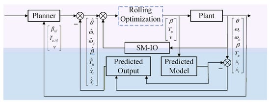
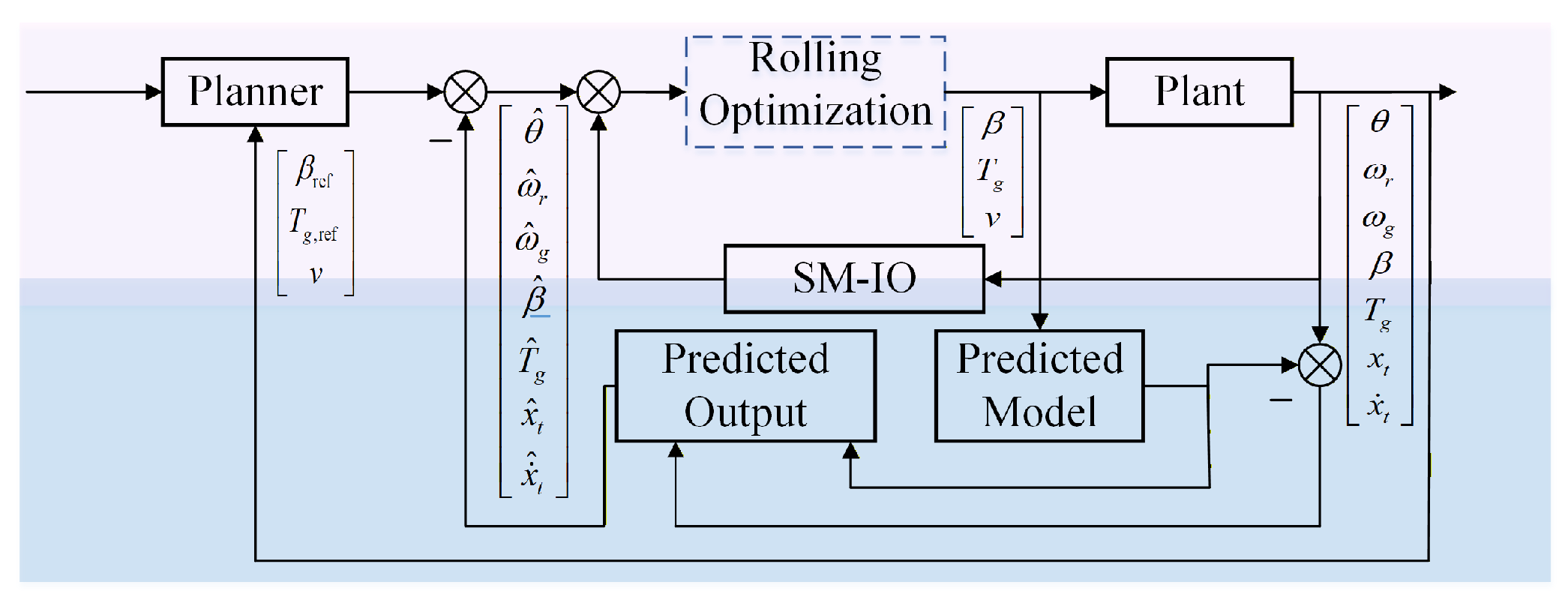
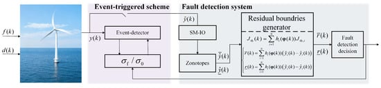
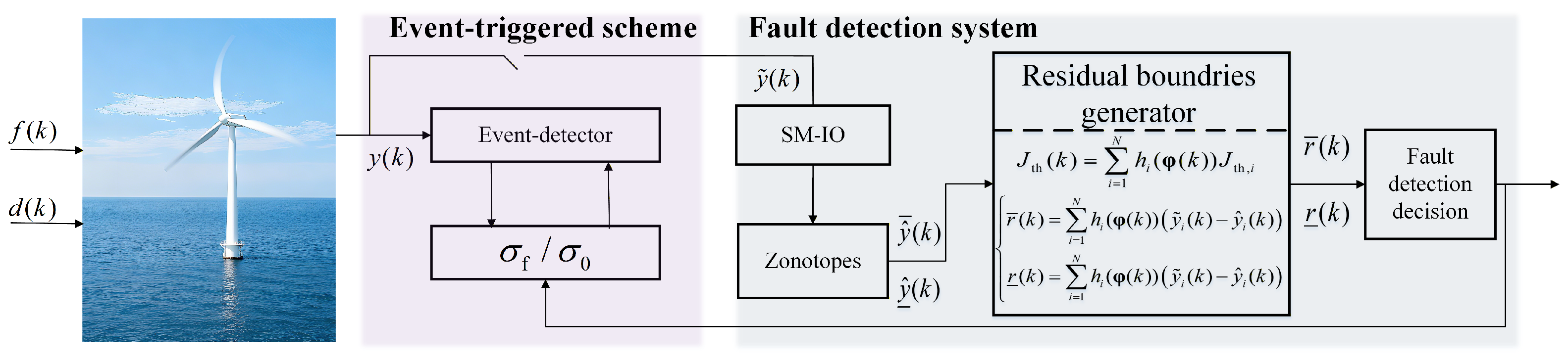
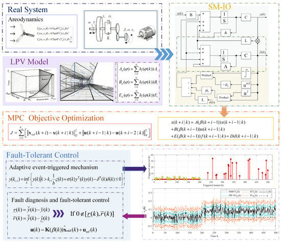
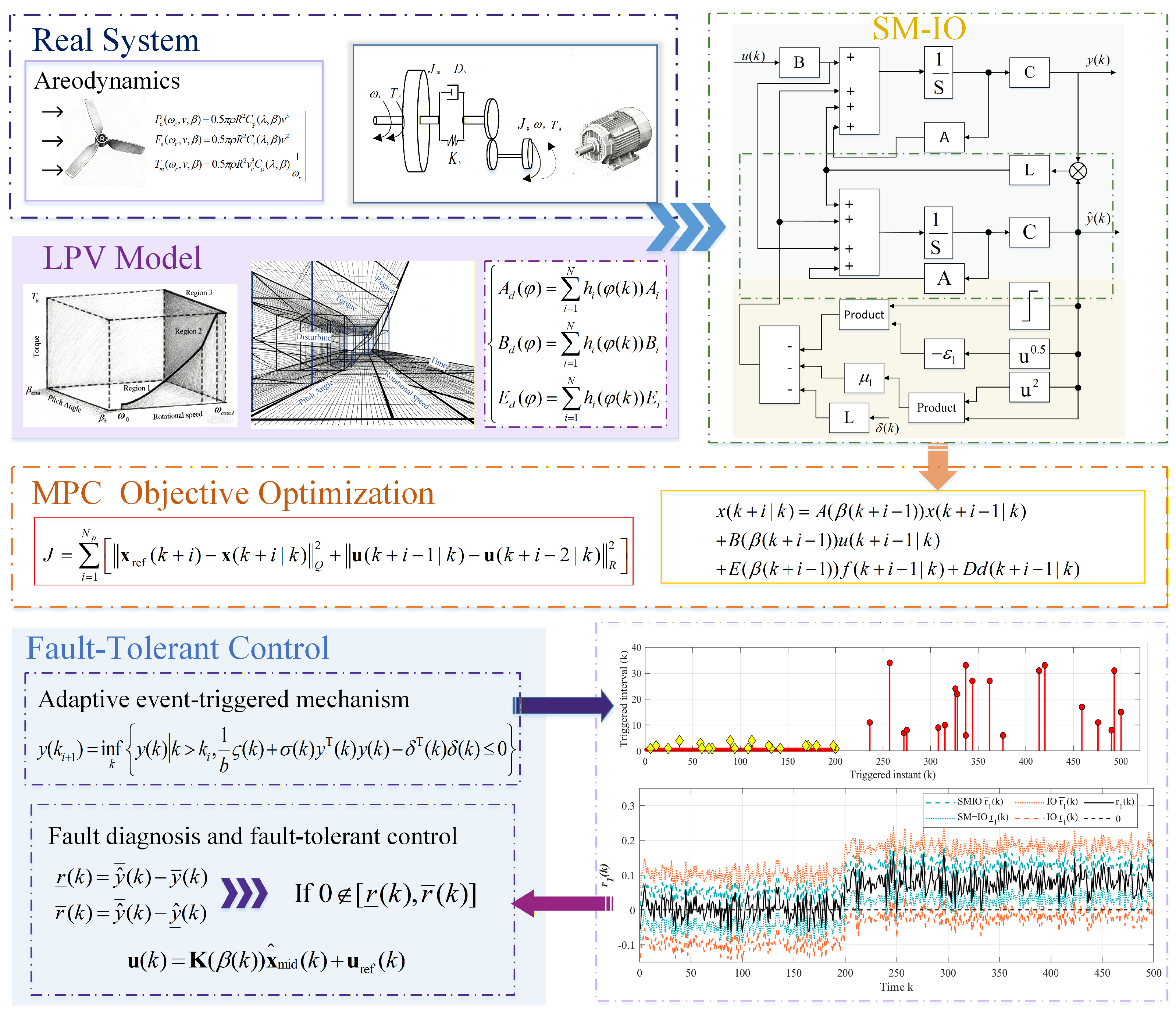
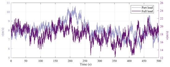
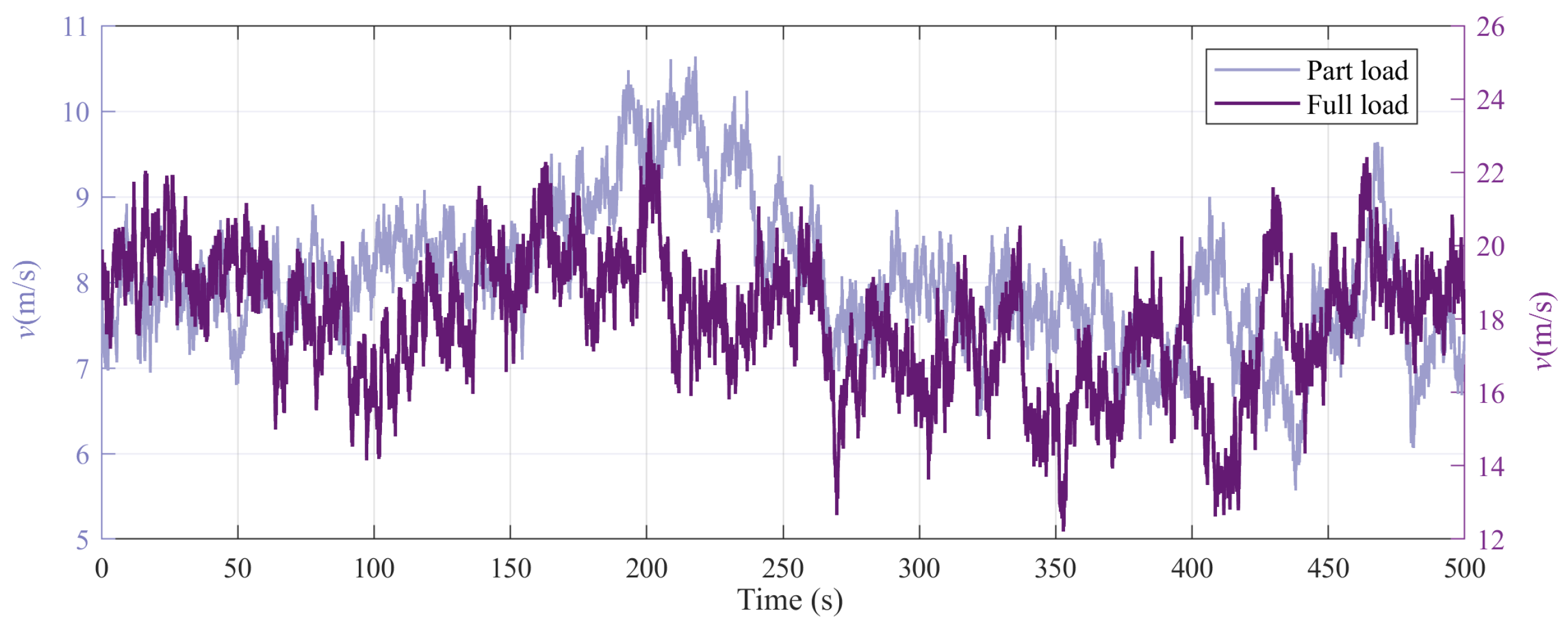
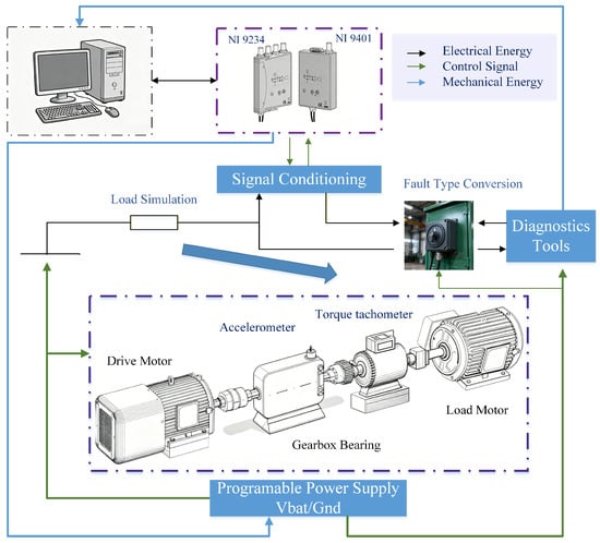
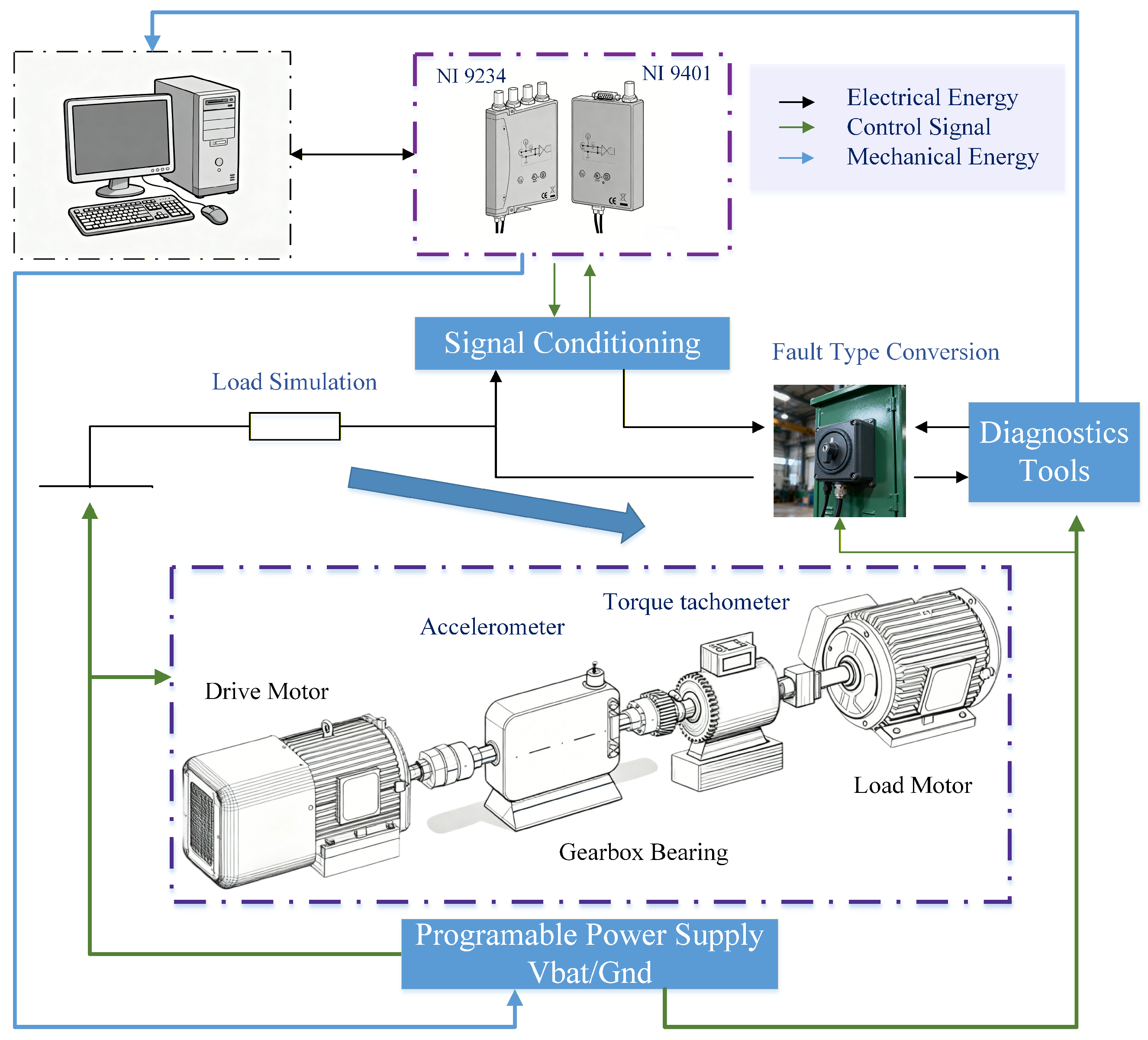
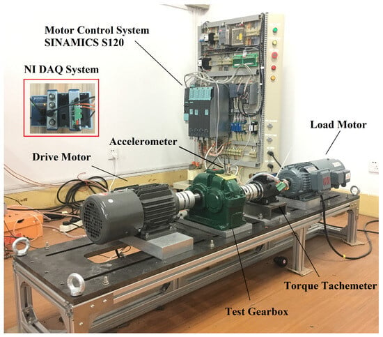
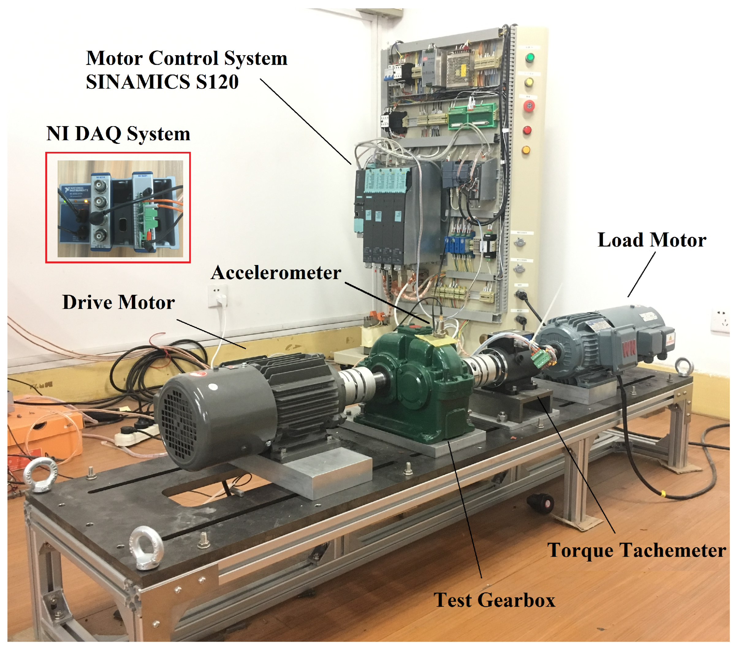
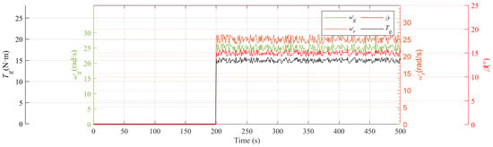
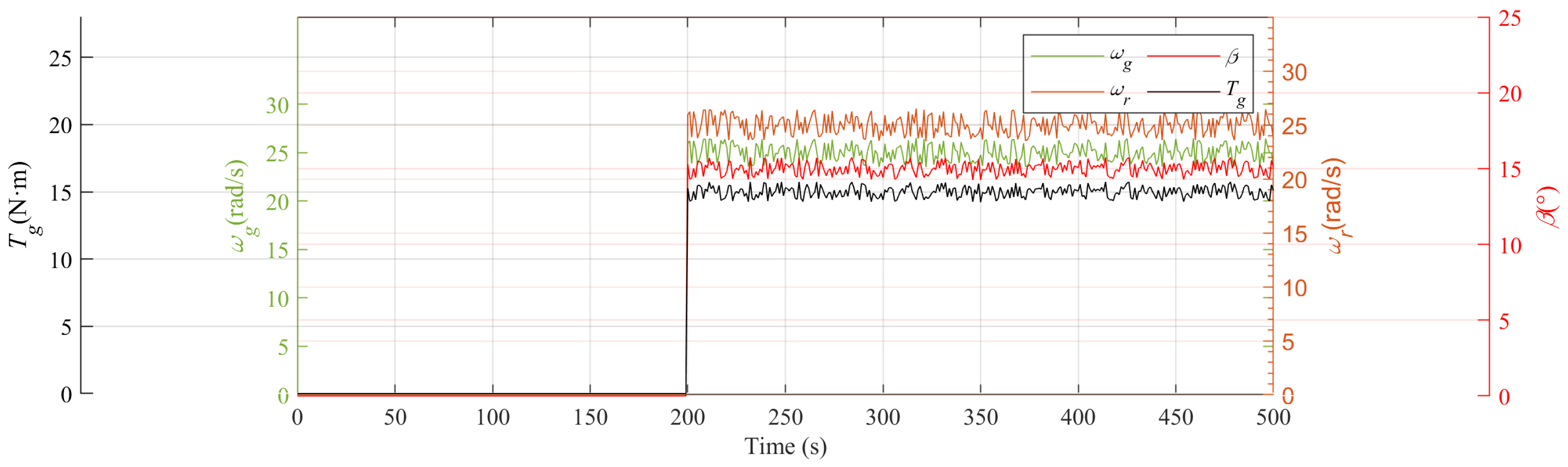
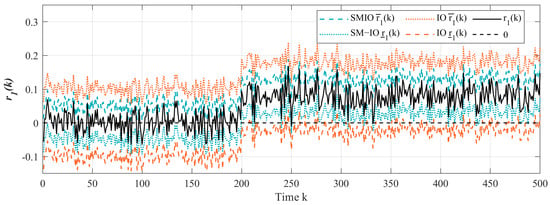
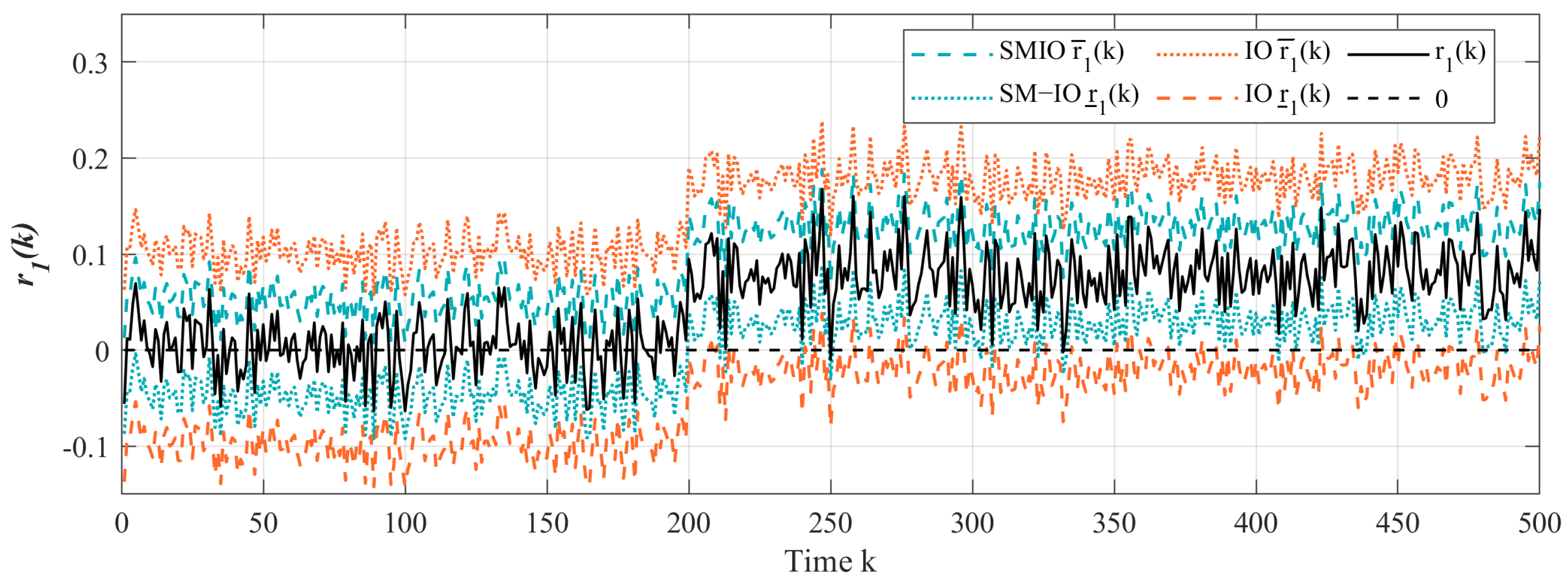
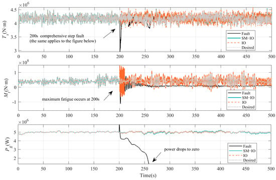
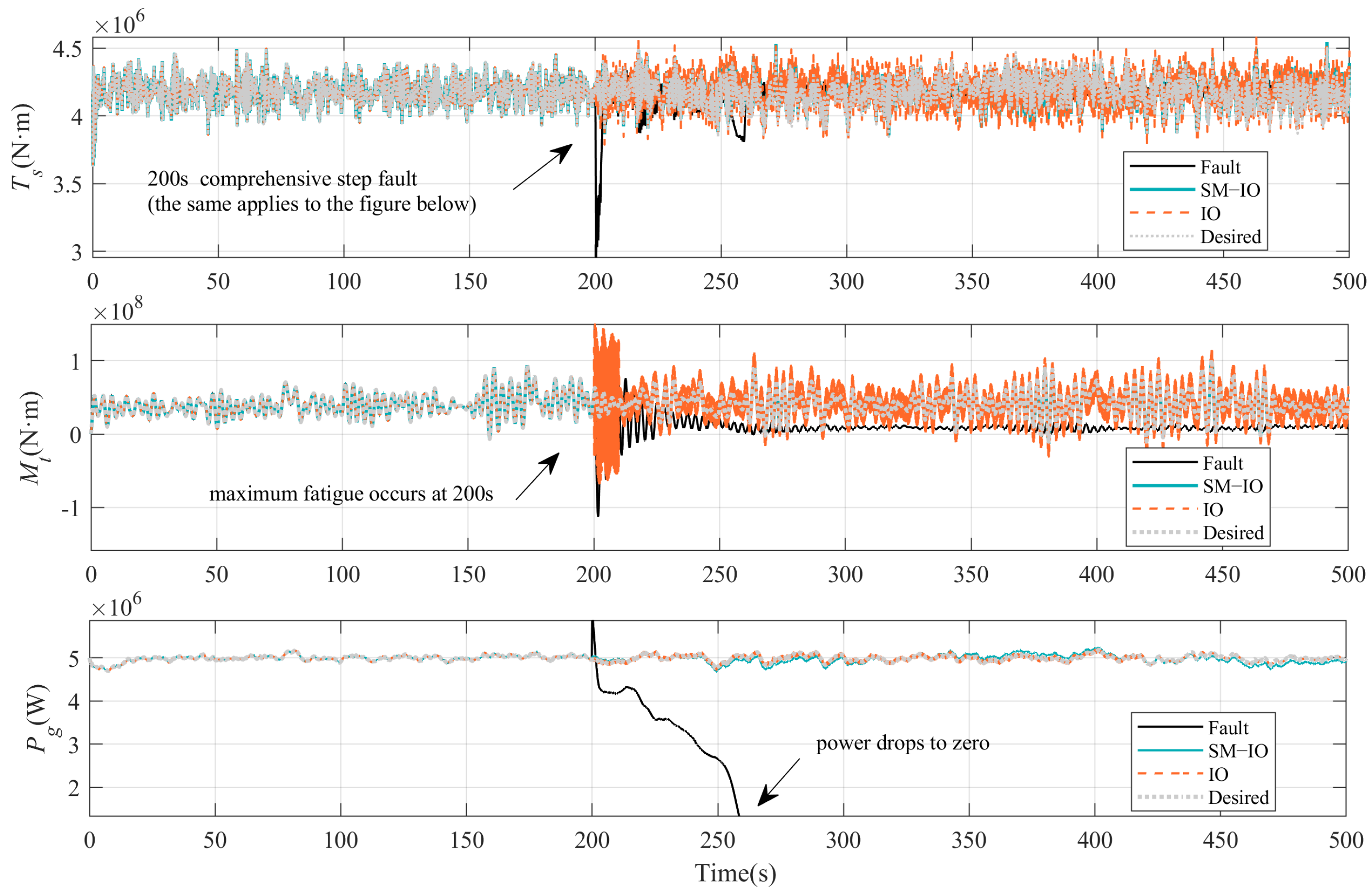
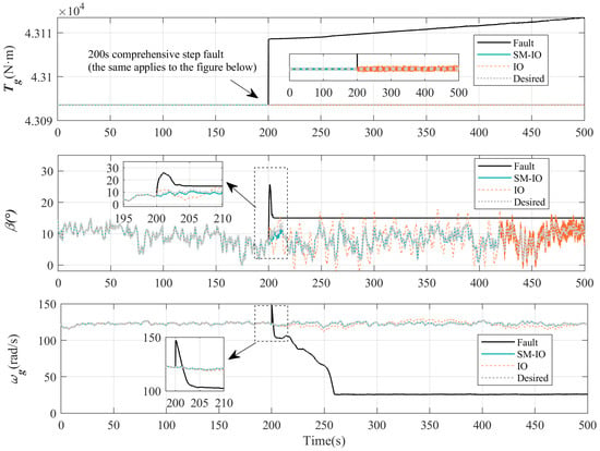
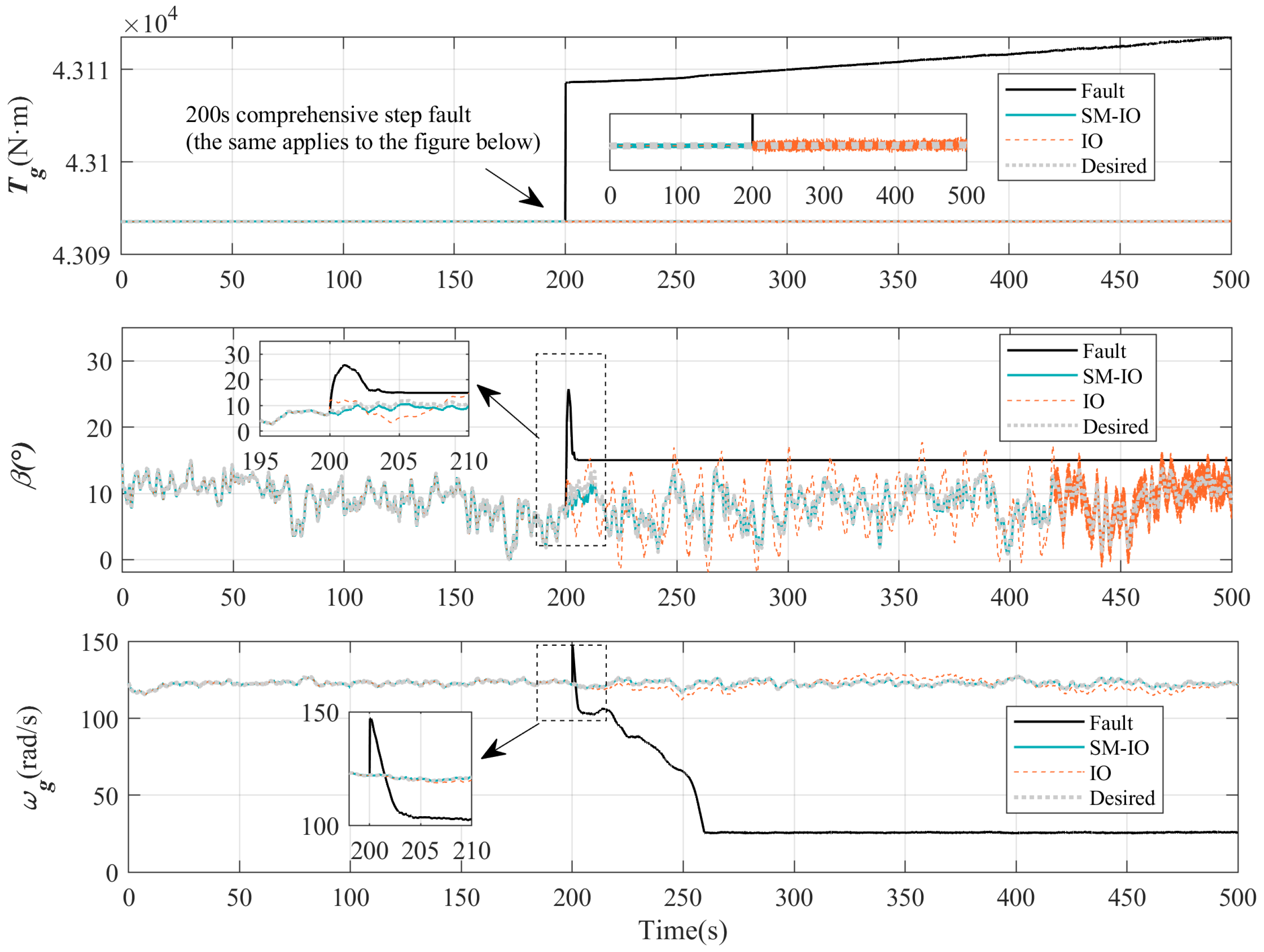
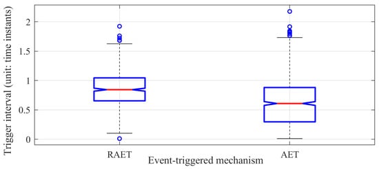
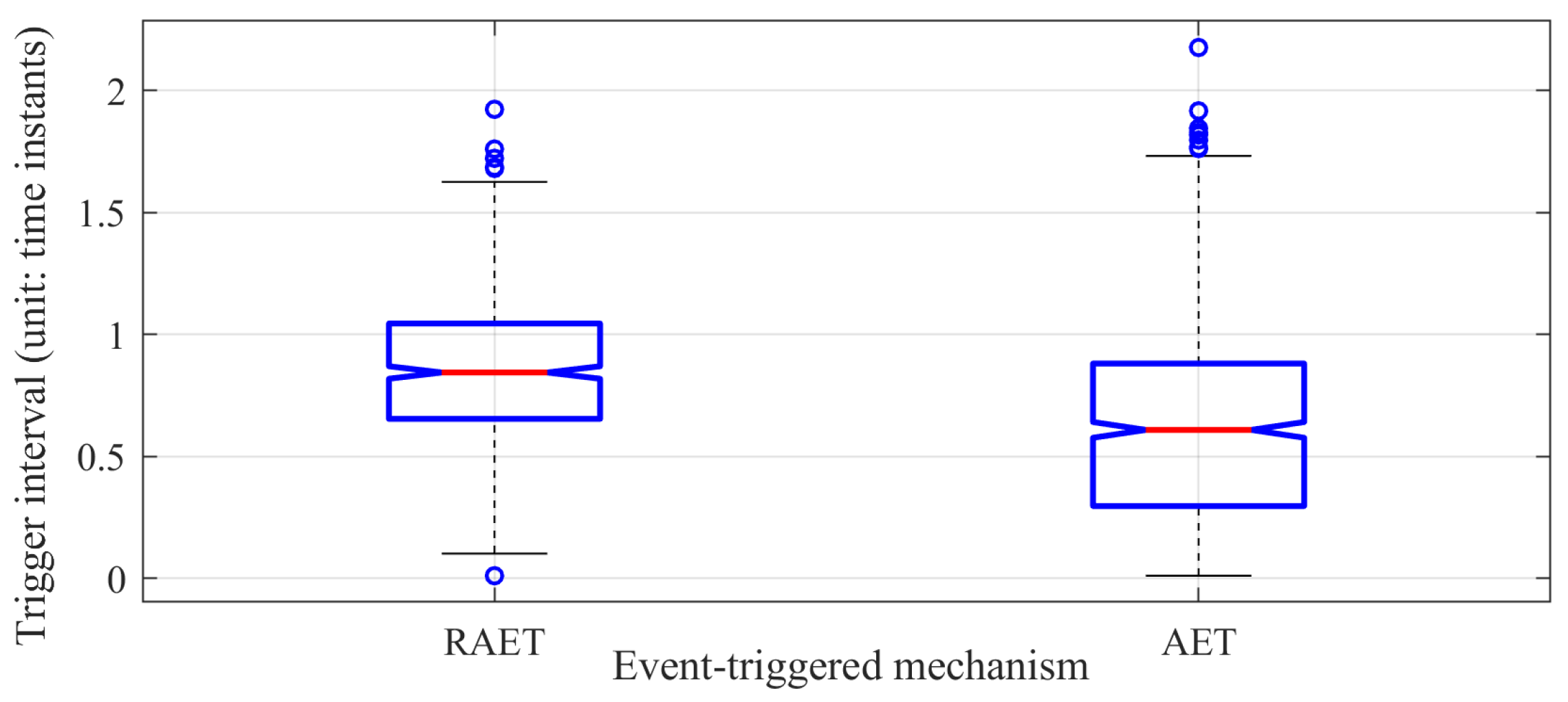
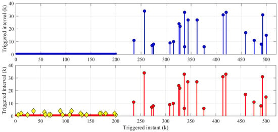
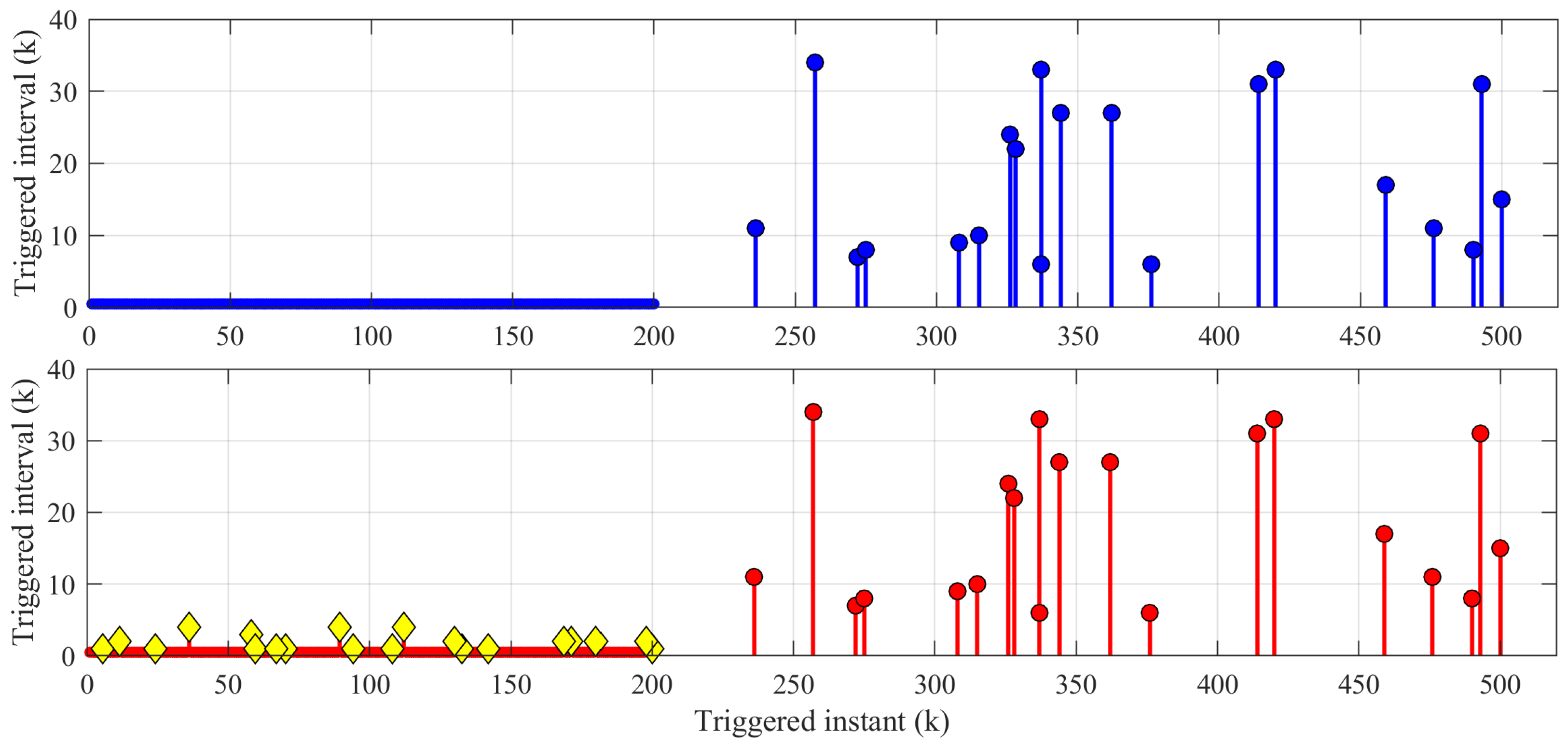
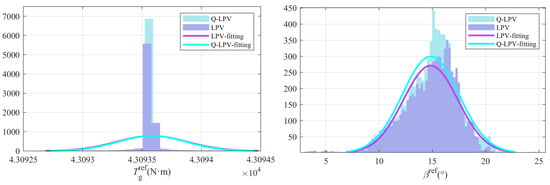
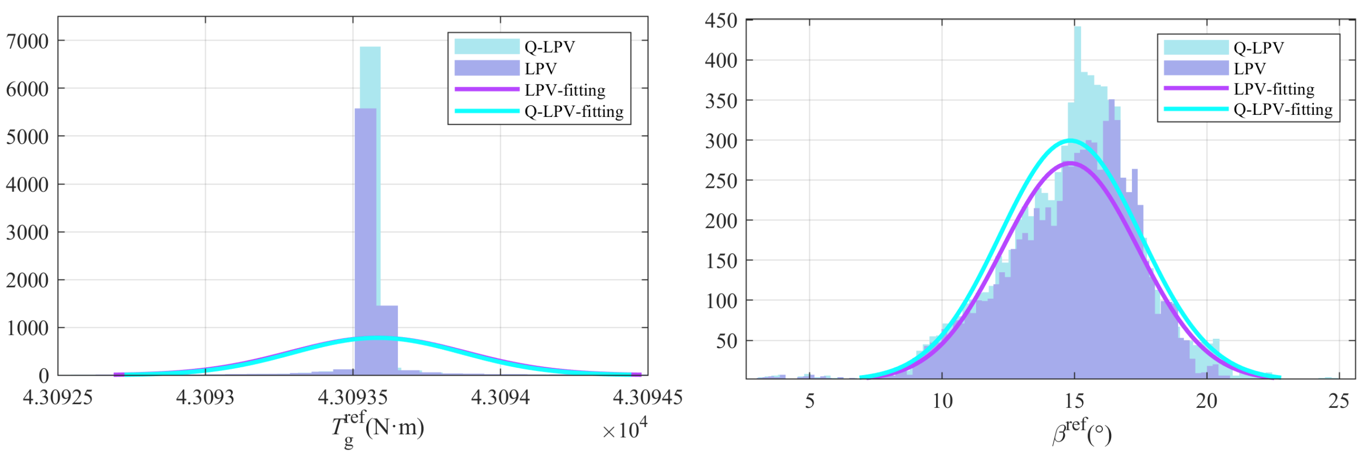
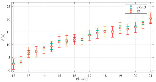
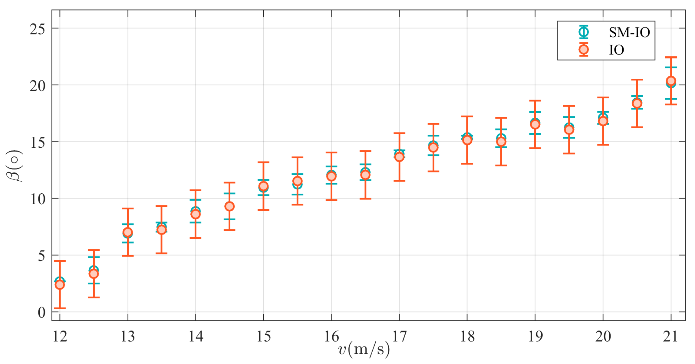
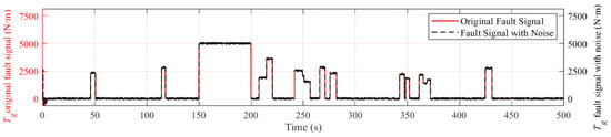
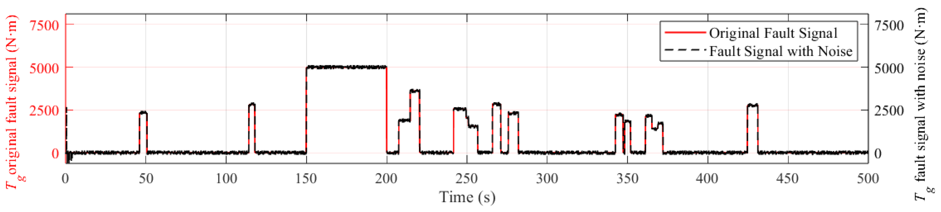
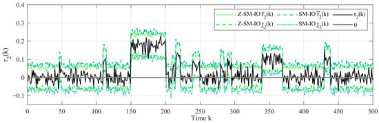
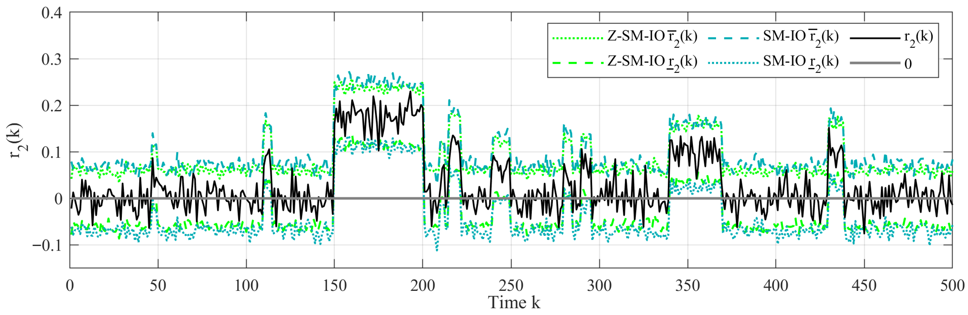
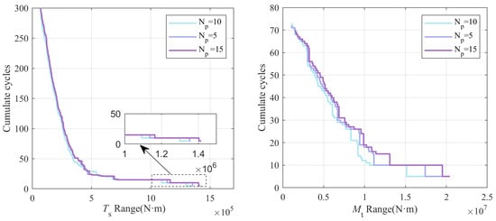
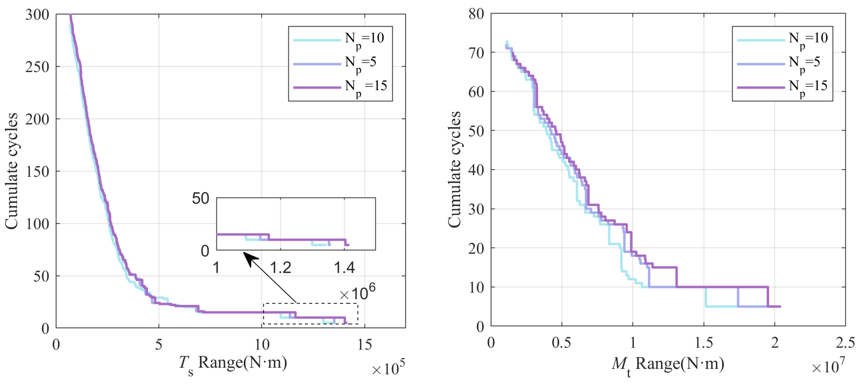
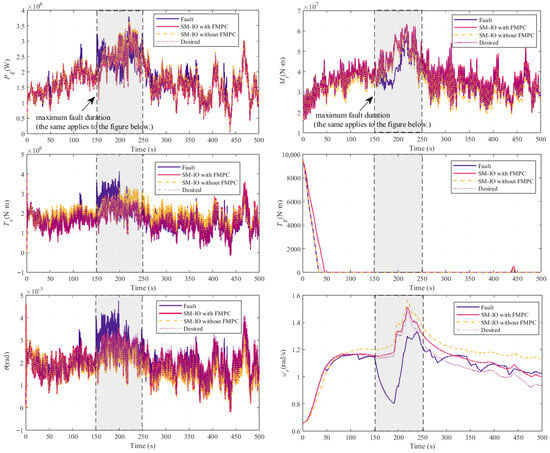
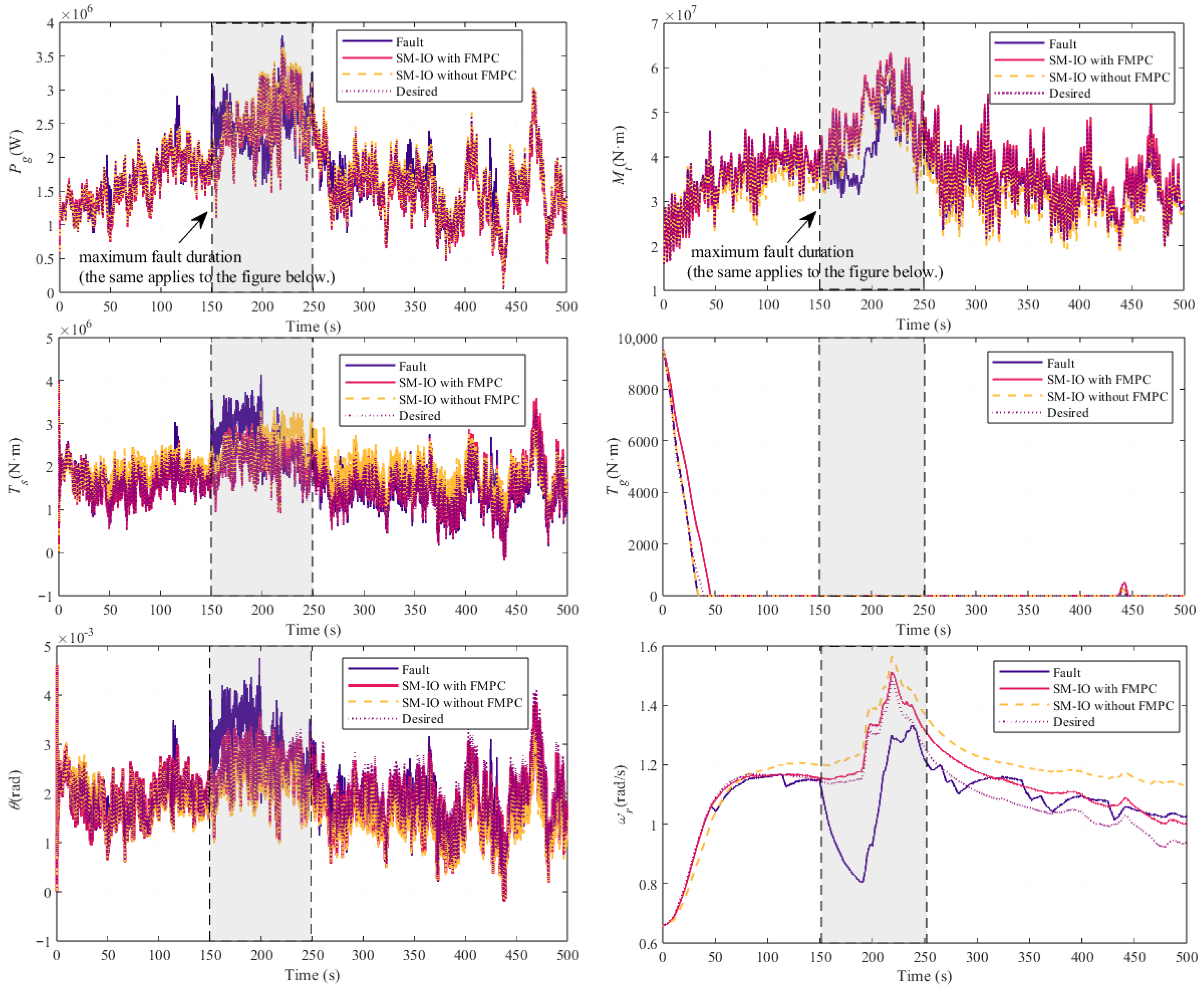
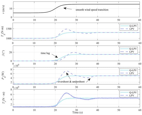
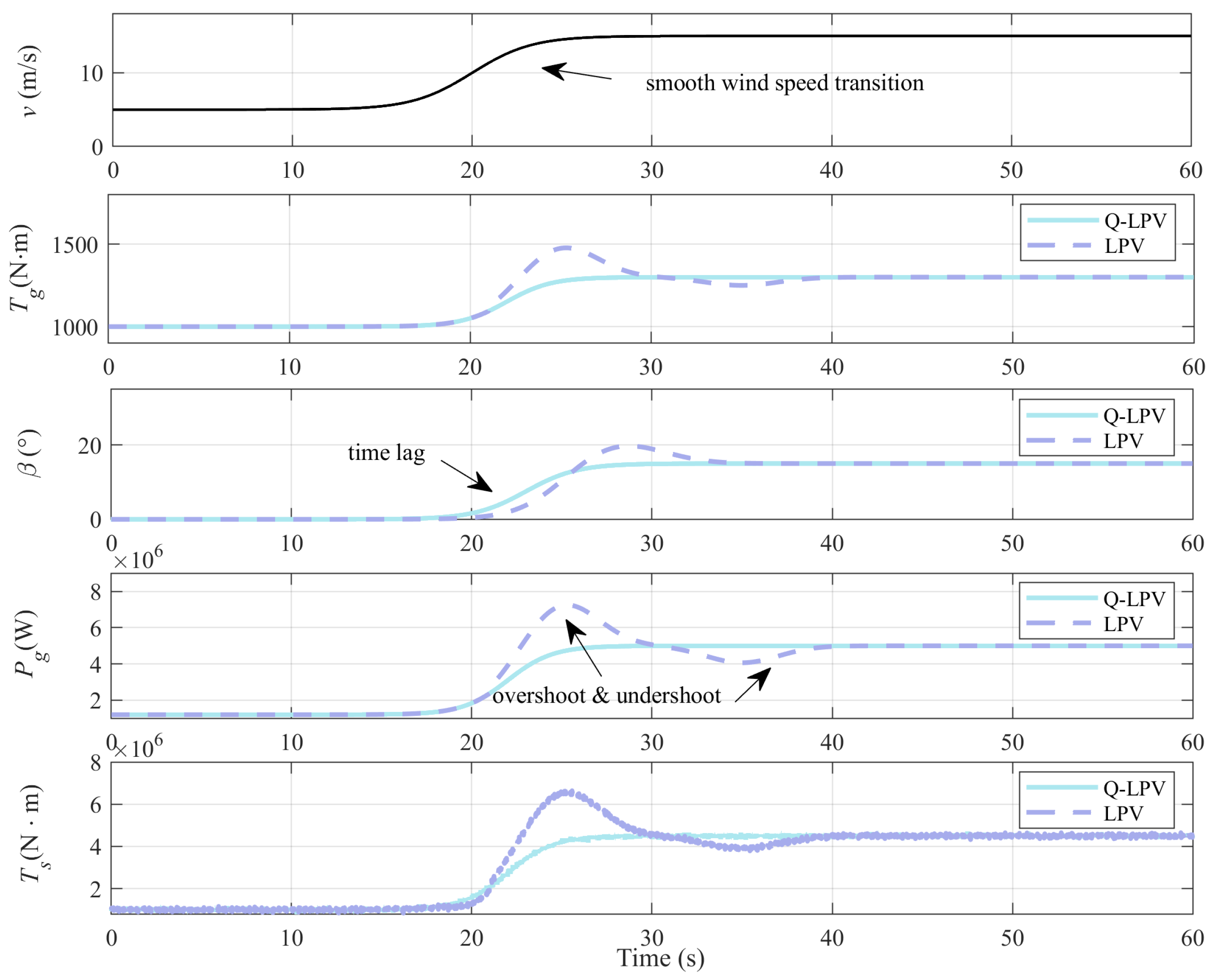
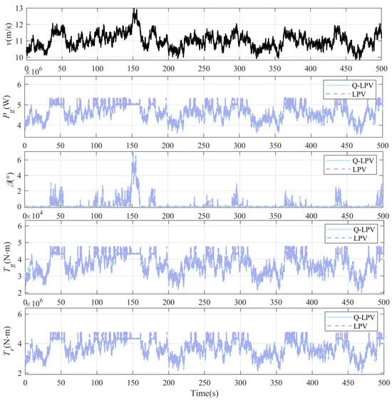
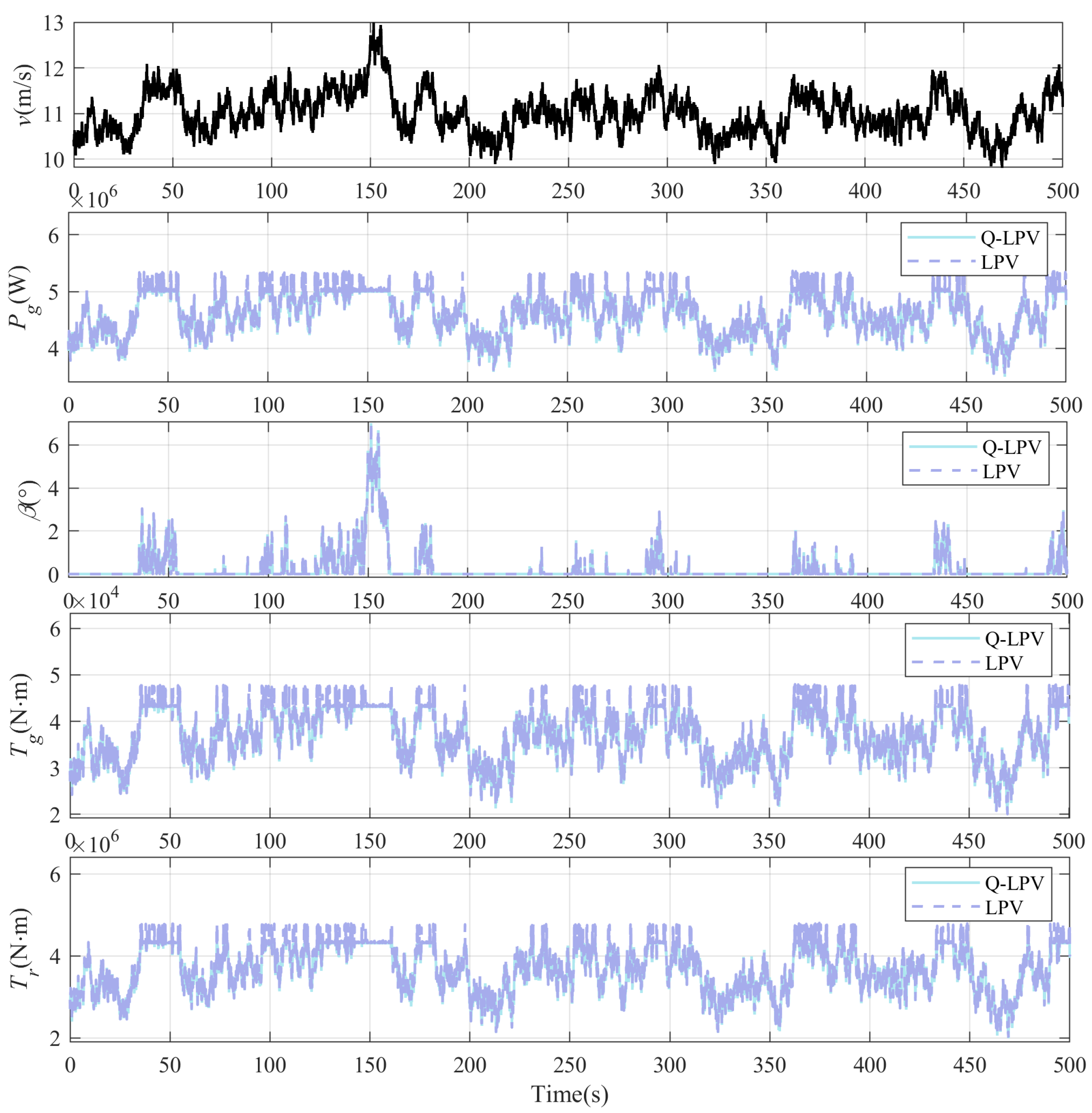

Disclaimer/Publisher’s Note: The statements, opinions and data contained in all publications are solely those of the individual author(s) and contributor(s) and not of MDPI and/or the editor(s). MDPI and/or the editor(s) disclaim responsibility for any injury to people or property resulting from any ideas, methods, instructions or products referred to in the content. |
© 2026 by the authors. Licensee MDPI, Basel, Switzerland. This article is an open access article distributed under the terms and conditions of the Creative Commons Attribution (CC BY) license.