


Abstract
Understanding the complex drivers of water yield is essential for ensuring basin water resource security, yet existing linear approaches often overlook the critical nonlinear effects arising from factor interactions. Previous studies combining the InVEST model with attribution methods have typically treated climate and land use as independent factors, failing to quantify their interactive effects beyond additive assumptions. This study addresses this gap by introducing a coupled framework that explicitly isolates and quantifies nonlinear climate–land interactions through scenario-based residual decomposition and spatial interaction detection. Focusing on the Minjiang River Basin, this study first applies a locally calibrated InVEST model to analyze the spatiotemporal patterns of water yield from 2000 to 2023. Through scenario analysis and the Geographical Detector method, we decoupled the contributions of climatic factors, land use, and their interactions. The results show significant spatiotemporal heterogeneity in water yield, averaging 1053.59 mm, with a spatial pattern aligned closely with precipitation. Climatic factors dominated the changes (average contribution 93.43%), while the direct contribution of land use was minimal (−1.56%). Importantly, a significant nonlinear interaction effect was identified (average 8.13%), with the interplay between precipitation and forest land proportion showing the strongest explanatory power for spatial differentiation (q-statistic up to 96.4%). These findings highlight the necessity of an integrated climate-land regulatory strategy that enhances climate resilience and optimizes key land uses to promote sustainable water management, providing a methodological framework for analyzing complex hydrological drivers.
1. Introduction
As the core process of water resource formation, the spatiotemporal evolution of basin water yield exerts a profound influence on regional water security, ecosystem health, and the sustainable development of society and the economy [1,2]. Under the dual pressures of global climate change and intensive human activities, clarifying the dominant drivers and mechanisms underlying water yield changes has become a frontier scientific issue in hydrology and water resource management [3]. Climatic factors—particularly precipitation and temperature—and land use are widely recognized as two key external stressors regulating water yield dynamics [4].
Traditional studies have mainly sought to quantify their individual contributions using statistical methods (e.g., multiple linear regression, elasticity coefficient method) or by comparing simulated results between baseline and altered periods [5,6,7]. However, these approaches typically rely on the linear assumption of factor independence, oversimplifying the attribution of total changes to the algebraic sum of individual factor contributions. In reality, climatic processes and land use changes do not act in isolation; instead, they generate nonlinear interactive effects through complex biogeophysical and hydrological feedback mechanisms [8,9,10,11]. Identical precipitation inputs can elicit significantly different runoff responses under varying vegetation cover [9], while land use changes such as deforestation or urbanization can further alter local climatic conditions (e.g., evapotranspiration), thereby synergizing with or offsetting macroscale climate change [10,11].
Most existing attribution frameworks still rely on linear decomposition methods that treat the contributions of individual factors as an algebraic sum, thus obscuring the synergistic or antagonistic nature of these interactions. Neglecting such nonlinear interactions not only masks the true contribution of each driver but may also lead to biased predictions of future hydrological regimes and inappropriate adaptive management strategies. Therefore, developing a research framework that can effectively decouple the independent effects of climate and land use while quantifying their nonlinear interactions is of great theoretical and practical significance for advancing the understanding of basin hydrological response mechanisms.
The Minjiang River Basin (MRB), the largest independent river system flowing into the sea in Fujian Province, serves as a critical regional water source and ecological barrier while also underpinning the province’s rapid socio-economic development [12]. In recent years, the basin has experienced notable climatic fluctuations—characterized by the uneven spatiotemporal distribution of precipitation and frequent extreme events—as well as significant land use transitions, such as urban expansion and ecological restoration projects [13,14,15]. Previous studies in this region have separately explored hydrological responses to climate change or the impacts of land use changes on hydrological processes [16,17,18,19]. To our knowledge, no study in this basin has systematically separated the independent contributions of climate and land use from their nonlinear interactive effects, nor has any research explicitly linked mathematical residual interactions with spatial interaction mechanisms.
To address these research gaps, this study takes the MRB as a case study, aiming to construct an integrated analytical framework combining process-based modeling, controlled scenario analysis, and statistical detection. This framework is designed to accurately quantify the independent contributions and nonlinear interactions of climatic factors and land use to the spatiotemporal evolution of water yield. Specifically, this study will: (1) employ the InVEST Water Yield model, calibrated with localized parameters, to precisely simulate the spatiotemporal dynamics of basin water yield from 2000 to 2023; (2) innovatively design a series of controlled variable scenarios (climate-change-only with fixed land use, and land-use-change-only with fixed climate) to isolate the pure climate effect, pure land use effect, and their interactive effect from the total water yield change; and (3) introduce the Geographical Detector model to quantitatively diagnose, from the perspective of spatial differentiation, the explanatory power of key driving factors (e.g., precipitation, temperature, and different land use types) and their interactions on the formation of the water yield spatial pattern.
This study is expected to achieve the following objectives: (1) reveal the spatiotemporal evolution characteristics of water yield in the MRB; (2) quantitatively decouple the independent and interactive contribution rates of climatic factors and land use to water yield changes; and (3) identify the key factors dominating the spatial differentiation of water yield and their nonlinear interaction mechanisms. Importantly, this study innovates by (i) moving beyond the linear assumption of factor independence through a combined scenario-detector framework that explicitly isolates interactive effects; (ii) quantifying the explanatory power of two-factor interactions (e.g., precipitation × forest) on spatial differentiation of water yield; and (iii) revealing that the nonlinear enhancement effect between climatic and land use factors, particularly forest and precipitation, plays a dominant yet previously underexplored role in hydrological spatial patterning. This framework provides a transferable paradigm for decoupling complex driver interactions in other basins facing similar environmental changes.
In this study, water yield refers to the annual amount of water exported from a pixel as runoff, calculated as precipitation minus actual evapotranspiration within the InVEST Water Yield model framework. It represents the potential hydrological supply from the landscape under natural conditions and does not account for anthropogenic water withdrawals, reservoir regulation, or groundwater–surface water interactions. Thus, it should be interpreted as an indicator of ecosystem water production capacity rather than net water available for direct human use.
2. Materials and Methods
2.1. Study Area
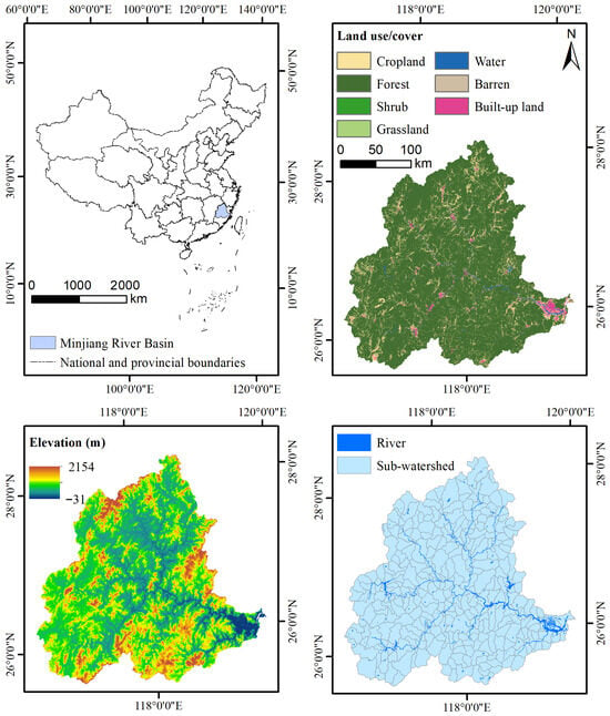
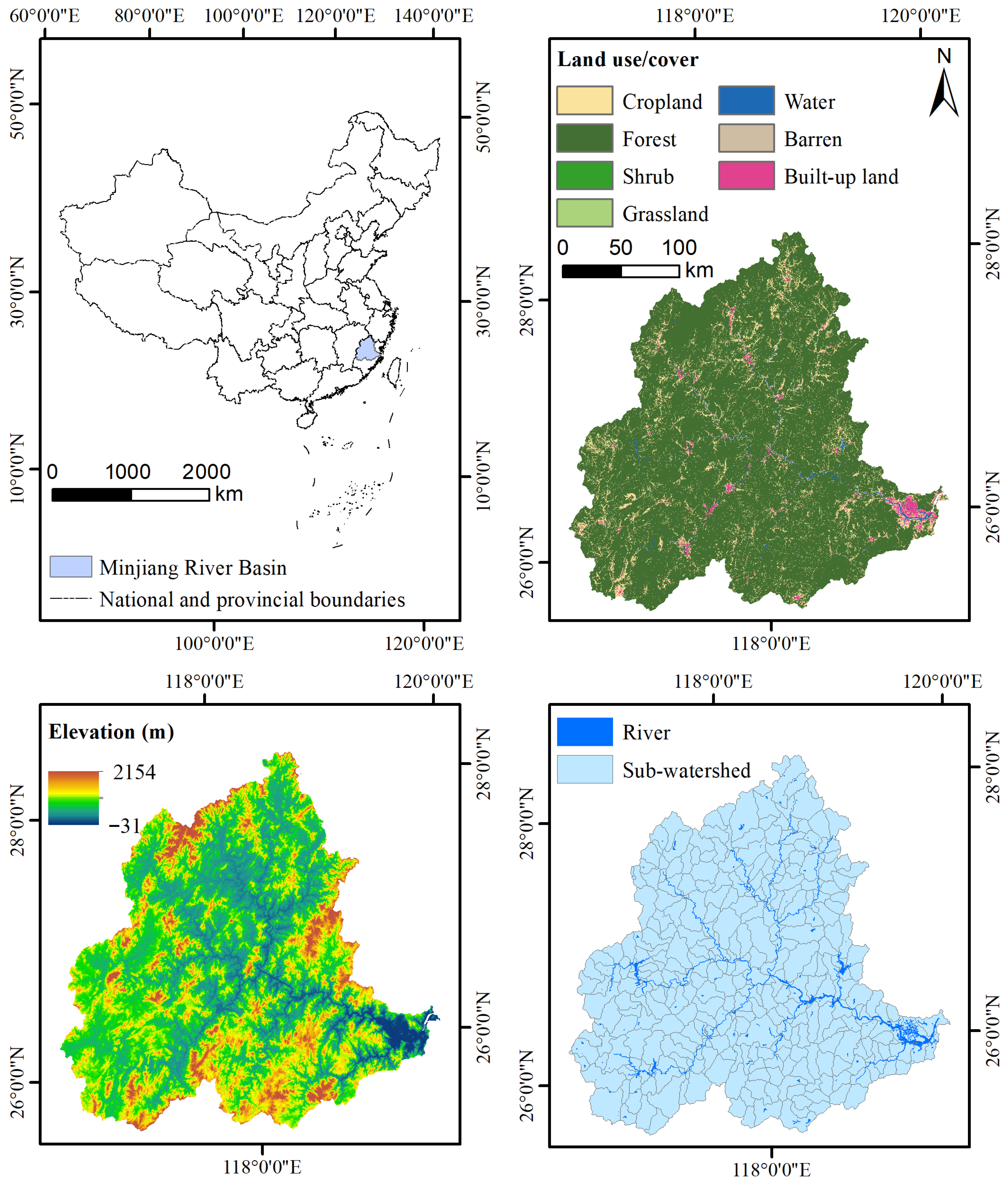
The MRB is situated on the southeastern coast of China (116°23′–119°35′ E, 25°23′–28°16′ N), with a drainage area of approximately 60,992 km2, accounting for roughly 50% of the total land area of Fujian Province (Figure 1) [20]. As the largest independent river system directly flowing into the sea within the province, it serves as a critical water source and ecological barrier, underpinning the regional socio-economic development [12]. The basin features a stepwise descending topographic gradient from the northwest to the southeast: the northwestern part is dominated by the steep Wuyi Mountains; the central region transitions to medium-low mountains and hills (e.g., the Daiyun Mountains); and the southeastern area gradually slopes down to the Fuzhou Plain and coastal zones [21].
Figure 1.
Location of the Minjiang River Basin in Fujian Province, China. The map shows the basin boundary, main river channels, and elevation gradient.
Climatically, the basin is governed by a subtropical monsoon climate, jointly influenced by maritime factors and topographic conditions, resulting in a warm and humid environment with abundant yet spatiotemporally heterogeneous precipitation [13]. The annual average precipitation ranges from 1500 to 2000 mm, with substantial interannual variability: the 1990s were a relatively wet period, while a declining trend in precipitation has been observed since the early 21st century [22]. Spatially, two major precipitation centers are formed on the southeastern slopes of the Wuyi Mountains and in the Daiyun Mountains area, where annual precipitation exceeds 2000 mm [19]. In contrast, the southeastern coastal plain receives relatively less precipitation, generally below 1600 mm [23].
The basin’s complex topography—ranging from steep mountainous headwaters to gently sloping coastal plains—creates strong gradients in precipitation, vegetation, and soil properties, making it an ideal natural laboratory for studying climate–land interactions. The upper reaches, dominated by forest cover, exhibit high water yield and strong hydrological regulation capacity, while the lower reaches, characterized by urban expansion and agricultural intensification, show altered runoff generation processes. These spatial contrasts in both climatic forcing and land surface characteristics provide a unique opportunity to quantify how the interaction between precipitation and land use types shapes the spatiotemporal evolution of water yield—a central objective of this study.
2.2. Data Requirements and Sources
The data required for this study mainly consist of meteorological, soil, land use, and watershed boundary datasets (Table 1), spanning the period from 2000 to 2023. To ensure spatial alignment across all datasets, meteorological and soil layers (original resolution: 1000 m) were resampled to 30 m using bilinear interpolation. This method preserves the continuous nature of climatic and soil variables while enabling pixel-wise integration with high-resolution land use data. However, it is important to acknowledge that downscaling does not introduce new information at the sub-kilometer scale; rather, it assumes spatial continuity of climate fields within each 1 km grid cell. Consequently, fine-scale (30 m) variability in simulated water yield is predominantly driven by land use and topographic attributes, which vary at higher spatial frequency. Potential inconsistencies among datasets from different national sources were minimized by selecting harmonized products (e.g., HWSD for soils) and cross-validating meteorological data against local station observations where available. These uncertainties are considered acceptable for the basin-scale analysis conducted in this study, as the primary focus is on relative changes and spatial patterns rather than absolute pixel-level precision.
Table 1.
Data names, descriptions, and sources.
2.3. Methodology
This study adopted the Water Yield module of the InVEST 3.14.2 model to simulate the spatiotemporal distribution of basin water yield. A multi-scenario controlled experiment was designed to disentangle the respective contributions of climatic factors and land use change. Subsequently, the Geographical Detector method was employed to quantify the explanatory power and interaction effects of various driving factors.
2.3.1. Water Yield Assessment
Based on the Budyko hydro-climatic coupling equilibrium theory and the water balance equation, the model simulates the allocation of precipitation among processes such as vegetation interception, soil infiltration, and evapotranspiration [24]. It is important to note that the InVEST Water Yield 3.14.2 model simulates the long-term average natural water balance at the pixel scale. The resulting water yield estimates represent the green and blue water flux leaving the pixel as runoff, excluding human consumptive uses and groundwater exchanges. This metric is therefore best understood as a biophysical indicator of hydrological ecosystem services. The core calculation formulas are as follows:
Annual water yield Y(x) for pixel x:
The ratio of actual evapotranspiration to precipitation:
Potential evapotranspiration PET(x):
Empirical parameter w(x) (related to plant-available water):
Plant-available water content AWC(x):
Plant-available water capacity PAWC (related to soil texture):
where Y(x) represents the annual water yield for pixel x (mm); AET(x) is the annual actual evapotranspiration (mm); P(x) denotes the annual precipitation (mm); and PET(x) signifies the annual potential evapotranspiration (mm). The symbol w is the dimensionless parameter of the Budyko curve; Kc(lx) refers to the vegetation evapotranspiration coefficient for land use type l at pixel x; and ET0(x) is the reference evapotranspiration (mm). Z indicates the Zhang coefficient, which characterizes precipitation seasonality (range: 1–30); AWC(x) is the plant-available water content (mm); and PAWC is the plant-available water capacity (mm). Finally, S%, Si%, C%, and OC% correspond to the soil sand, silt, clay, and organic carbon content percentages, respectively.
2.3.2. Calibration and Validation
The seasonal constant Z (Zhang coefficient) ranges from 1 to 30. Model simulations were calibrated and validated against observed runoff depth data from the Fujian Provincial Water Resources Bulletin. According to the Budyko aridity index theory, the influence of the Z value on model results diminishes as its value increases.
2.3.3. Scenario Design for Contribution Rate Separation
To clarify the differences in climatic inputs across scenarios, we summarized the annual mean precipitation, potential evapotranspiration, and major land use proportions for each scenario year (Table 2). For example, compared to 2000, precipitation increased by 18.20% in 2010 but decreased by 15.21% in 2020; forest area decreased by 3.81% and built-up area increased by 0.87% over the 23-year period. These actual change characteristics provide the basis for scenario settings and help interpret the simulated water yield responses.
Table 2.
Actual changes in climatic factors and land use conditions from 2000 to 2023.
To quantify the individual and interactive impacts of climatic factors and land use change, ten scenarios were designed (Table 3). The Baseline Scenario utilized actual climatic and land use data from the year 2000.
Table 3.
Scenario design for climatic variables and land use change.
Climatic Factor Change Scenarios (Scenarios 1–5): Land use was fixed at the 2000 condition (control variable), while climate data were replaced with datasets from 2005, 2010, 2015, 2020, and 2023, respectively (changing variable). This isolates the effect of pure climatic change on water yield.
Land Use Change Scenarios (Scenarios 6–10): Climatic factors were fixed at the 2000 condition (control variable), while land use data were replaced with datasets from 2005, 2010, 2015, 2020, and 2023, respectively (changing variable). This isolates the effect of pure land use change on water yield.
Contribution rates of different drivers were calculated by comparing water yield changes (ΔW) under the following scenarios:
where Rc, Rl, and Ri are the contribution rates of climatic factor change, land use change, and their interaction to the spatiotemporal evolution of water yield, respectively; ΔWt is the total change in water yield between two periods, caused by the combined change in climate and land use; ΔWc is the change in water yield attributable solely to climatic factor change, derived from Scenarios 1–5; and ΔWl is the change attributable solely to land use change, derived from Scenarios 6–10.
Nature of the interaction term: The interaction contribution (Rᵢ) derived from Equation (9) is a residual-based estimate—the portion of total water yield change that cannot be linearly attributed to either climate or land use alone. This residual captures the net effect of all nonlinear feedbacks, synergies, and antagonisms between the two drivers, but does not physically isolate specific interaction mechanisms. Similar residual-based approaches have been widely used in hydrological attribution studies, yet they remain subject to the limitation that the residual may also encapsulate model structural errors or unaccounted factors. In this study, we mitigate this limitation by cross-validating the residual interaction signals with independently derived spatial interaction metrics from the Geographical Detector (Section 2.3.4), thereby providing a more robust interpretation of nonlinear effects.
Interpretation of rates exceeding 100%: Contribution rates are expressed relative to the total observed change (ΔWt). When Rc exceeds 100%, this indicates that the climate-only effect alone would have produced a larger change than the total observed change, but this was partially offset by negative land use and/or interaction effects. In other words, the total change is the net result of a large positive climate effect counterbalanced by antagonistic land use and interaction effects. This does not imply that climate physically contributes more than 100% of the change, but rather reflects the non-additive nature of the system where drivers interact to produce a net outcome smaller than the sum of their individual effects. This interpretation is consistent with the negative interaction contributions observed in the same periods.
Justification and limitations of the fixed-baseline replacement approach: The scenario design using a fixed baseline (2000) with replacement years follows established practices in hydrological attribution studies, where isolating pure climate and pure land use effects requires controlling one factor while varying the other. This approach effectively captures first-order sensitivities and is computationally efficient for multi-temporal comparisons. However, we acknowledge its inherent coarseness: (1) it assumes that the baseline year is representative of initial conditions; (2) it does not capture gradual, continuous change trajectories; and (3) the interaction term (Ri) is derived as a residual, which may also encapsulate model structural errors or unaccounted factors. To mitigate these limitations, we: (a) use multiple replacement years spanning different climate regimes (wet, dry, average); (b) cross-validate the residual interaction signals with independently derived spatial interaction metrics from the Geographical Detector (Section 2.3.4); and (c) interpret contribution rates as relative measures of proportional attribution rather than absolute physical shares. This multi-method triangulation enhances confidence in the identified interaction effects.
2.3.4. Geographical Detector
The Geographical Detector was used to quantitatively reveal the driving mechanisms of climatic and land use factors on the spatial differentiation of water yield [25]. This method is particularly suited for analyzing spatial stratified heterogeneity and quantifying the explanatory power of both individual factors and their interactions without assuming linear relationships.
The factor detector assesses the explanatory power of a single factor (e.g., precipitation, forest proportion) on the spatial variation in water yield. The explanatory power is measured by the q-statistic, calculated as
where q ranges from 0 to 1, with larger values indicating stronger explanatory power of the factor for the spatial differentiation of water yield; h = 1…L represents the stratification of the factor; Nh and σh2 are the number of samples and variance within stratum h, respectively; N and σ2 are the total number of samples and total variance across the study area; SSW is the within-stratum sum of squares; and SST is the total sum of squares.
The interaction detector evaluates whether two driving factors (X1 and X2; e.g., precipitation and temperature) exhibit nonlinear enhancement, weakening, or independence when jointly influencing water yield (Y) [26]. The core method involves comparing the single-factor q values, q(X1) and q(X2), with the interactive q value q(X1 ∩ X2). The type of interaction is then determined based on the relationships among these three values (e.g., nonlinear enhancement if q(X1 ∩ X2) > q(X1) + q(X2)).
A comprehensive set of driving factors was selected to capture both climatic and land surface influences on water yield:
Climatic factors: Precipitation (Precip), evapotranspiration (ET), mean temperature (Mean Temp), maximum temperature (Max Temp), and minimum temperature (Min Temp).
Land use factors: Proportions of cropland (CR), forest (FR), grassland (GR), and built-up land (BR), as well as the Normalized Difference Vegetation Index (NDVI).
Soil factor: Plant Available Water Capacity (PAWC), included as a static underlying surface factor to account for the influence of soil water holding capacity on spatial water yield patterns.
It is important to clarify the distinction between NDVI and vegetation-based land use proportions. While conceptually related, these variables capture different aspects of surface vegetation characteristics: land use proportions represent the areal extent of land cover types, whereas NDVI reflects the greenness and photosynthetic activity within those classes. NDVI can vary significantly even within the same land use type due to differences in species composition, growth stage, and health, thereby providing complementary information.
To ensure statistical robustness, multicollinearity diagnostics were performed using the Variance Inflation Factor (VIF). All variables included in the detector analysis exhibited VIF < 5, indicating that collinearity does not compromise the stability of the q-statistic estimates.
3. Results
3.1. Calibration and Validation of the InVEST Model
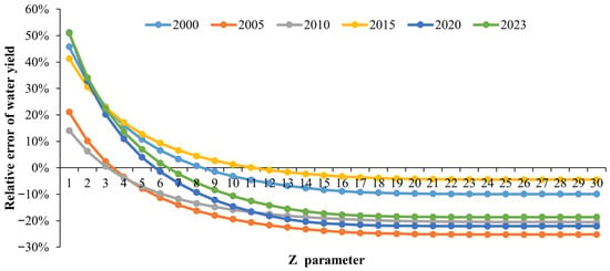
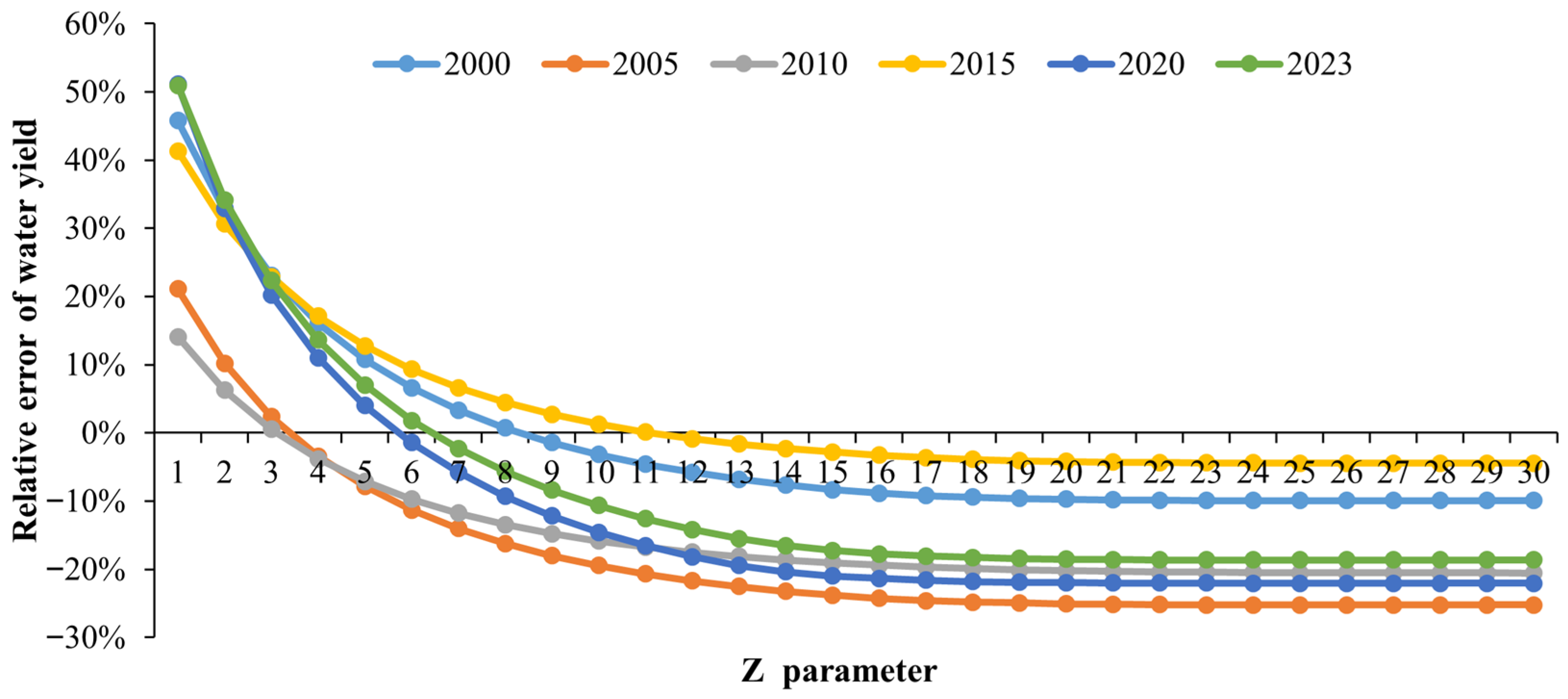
The InVEST model demonstrated strong applicability in the MRB (Figure 2, Table 4). Calibration focused on the seasonal parameter Z, which ranges from 1 to 30 and exerts a significant influence on simulation results. Through systematic testing, we identified Z = 6 as the optimal parameter for this basin. As Z increased from low to high values, the relative error decreased rapidly, reached a minimum at Z = 6, and then increased slightly before stabilizing—confirming Z = 6 as the most appropriate choice.
Figure 2.
Sensitivity of the InVEST model to the seasonal parameter Z. The plot shows the relative error between simulated and observed water yield for Z values ranging from 1 to 30, for each year from 2000 to 2023.
Table 4.
Optimal Z parameter and relative error of water yield from 2000 to 2023.
Following calibration, the model achieved high accuracy across all validation years. The average relative error of simulated water yield was only 1.04%, corresponding to a mean accuracy of 98.96%. To further assess model performance, we calculated the Nash–Sutcliffe Efficiency (NSE) and coefficient of determination (R2) using the six paired observations and simulations (2000, 2005, 2010, 2015, 2020, 2023). The resulting NSE of 0.9978 and R2 of 0.9983 indicate that the calibrated model not only minimizes bias but also accurately captures interannual variability in water yield.
Observed runoff depth values used for calibration and validation were obtained from the Fujian Provincial Water Resources Bulletin (2000–2023). This official publication reports basin-wide average runoff depths calculated from a network of hydrological stations operated by the provincial water resources department. These data are considered authoritative and representative of basin-scale hydrological conditions, providing a reliable reference for model calibration.
3.2. Spatiotemporal Evolution Characteristics of Water Yield
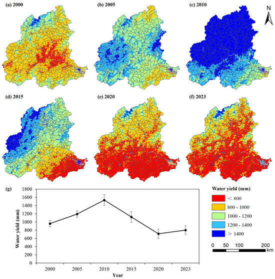
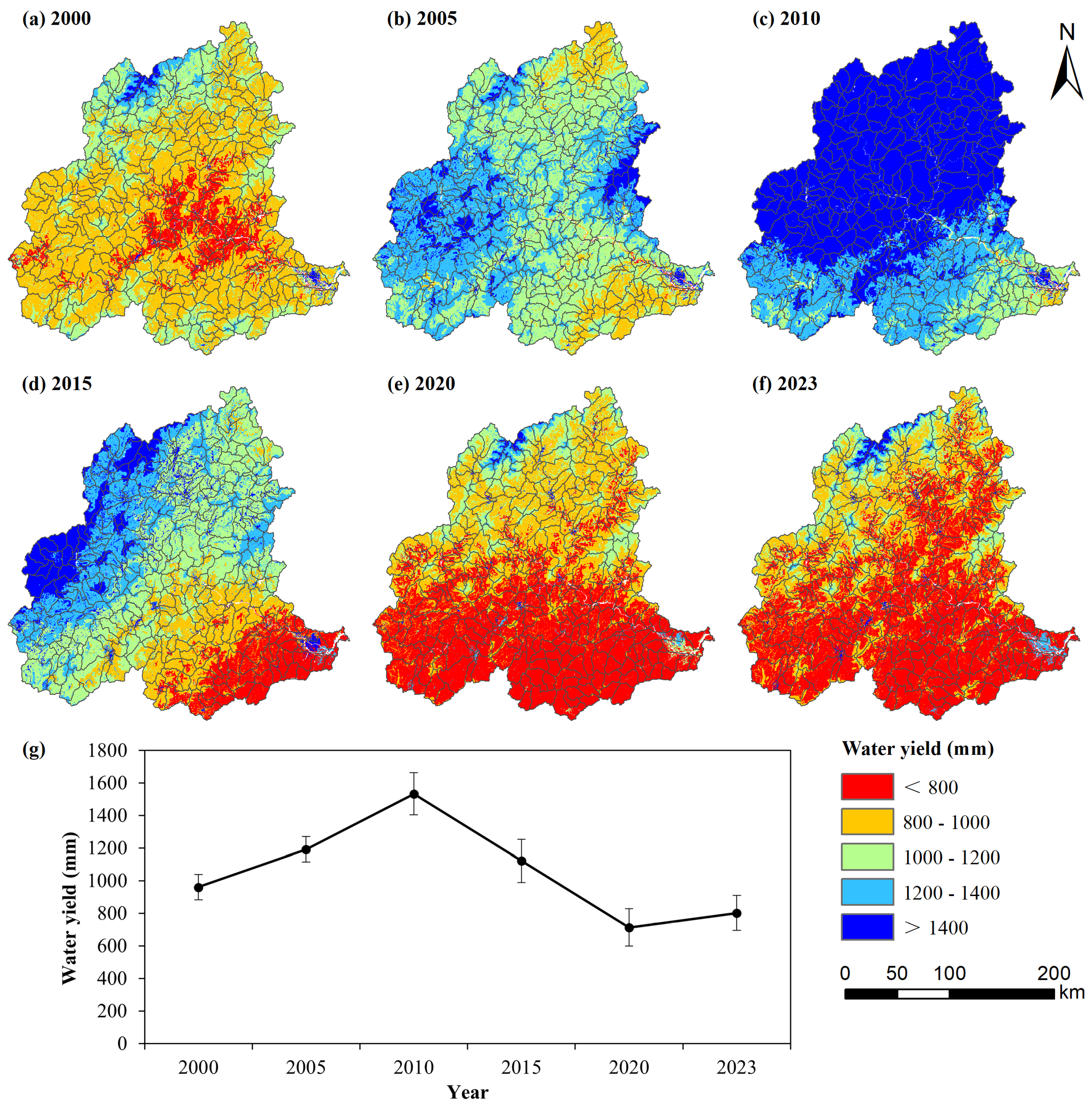
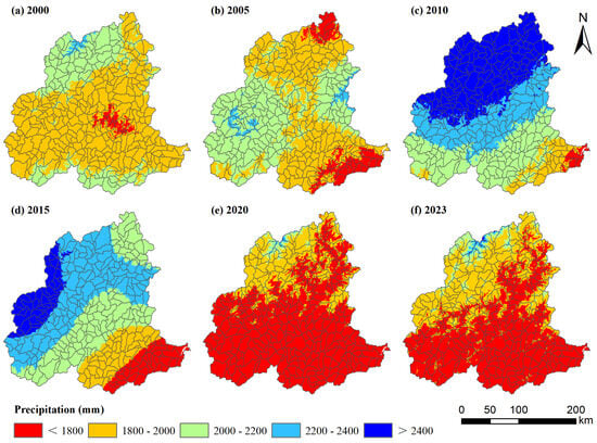
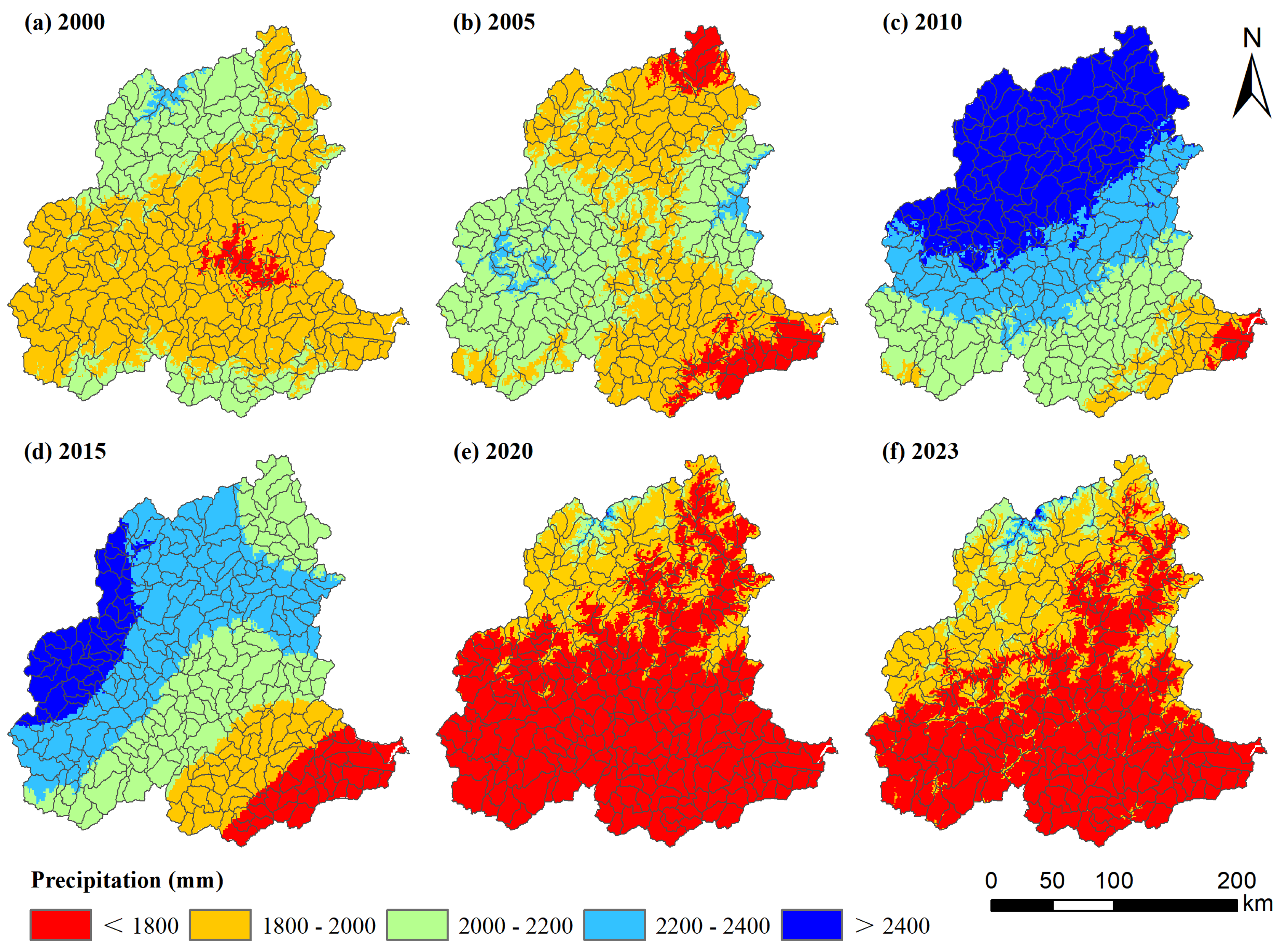
From 2000 to 2023, water yield in the MRB exhibited significant spatiotemporal heterogeneity (Figure 3), with a distribution pattern closely aligned with precipitation (Figure 4). The multi-year average water yield was 1053.59 mm. The highest value occurred in 2010 (1532.71 ± 260.40 mm), while the lowest was recorded in 2020 (713.18 ± 230.89 mm). Water yields in 2000, 2020, and 2023 fell below the multi-year average, whereas those in 2005, 2010, and 2015 exceeded it.
Figure 3.
Spatiotemporal patterns of water yield in the Minjiang River Basin from 2000 to 2023, simulated by the calibrated InVEST model. (a–f) represent the spatial distribution for the years 2000, 2005, 2010, 2015, 2020, and 2023, respectively; (g) represents the line graph with error bars.
Figure 4.
Spatiotemporal patterns of precipitation in the Minjiang River Basin from 2000 to 2023.
Spatially, a pronounced “high in the northwest and low in the southeast” pattern emerged. High-yield areas (>1400 mm) were predominantly distributed in the upper reaches of the basin, while low-yield areas (<800 mm) were concentrated in the middle and lower reaches. This spatial pattern is not solely driven by precipitation but is also modulated by topography and land surface characteristics. The high-yield areas in the upper reaches coincide with the Wuyi Mountains, where steep slopes and extensive forest cover enhance orographic precipitation and reduce evapotranspiration losses due to lower temperatures. Conversely, the low-yield areas in the middle and lower reaches are characterized by gentler topography, higher temperatures, and a mixture of cropland and urban land uses, which increase evapotranspiration and reduce runoff generation efficiency. The 2010 peak water yield corresponds to an exceptionally wet year, while the 2020 minimum reflects a dry year combined with continued urban expansion. This coupling between climatic variability and land surface properties underpins the nonlinear interactions explored in subsequent sections.
To quantitatively assess the influence of precipitation on water yield patterns, we conducted a spatial correlation analysis between water yield and annual precipitation for each year. The results reveal consistently high Pearson correlation coefficients: r = 0.903 (2000), 0.951 (2005), 0.985 (2010), 0.969 (2015), 0.957 (2020), and 0.935 (2023), with corresponding R2 values ranging from 0.82 to 0.97. These strong correlations confirm that precipitation is the dominant spatial control on water yield, consistent with the InVEST model structure. However, deviations from perfect correlation (R2 < 1) indicate that land surface characteristics—particularly vegetation cover, soil properties, and topography—modulate the precipitation-runoff relationship. Notably, the correlation was highest in 2010 (r = 0.985), the wettest year, suggesting that under extreme wet conditions, precipitation overwhelms local surface controls. In contrast, the slightly lower correlations in 2020 (r = 0.957) and 2023 (r = 0.935) reflect a greater relative influence of land surface heterogeneity under drier conditions. This interaction between precipitation and land surface properties is precisely the nonlinear effect that this study aims to quantify.
3.3. Contributions of Climatic Factors and Land Use Change to Water Yield Variation
3.3.1. Impact of Climatic Factor Changes
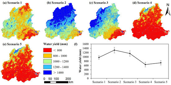
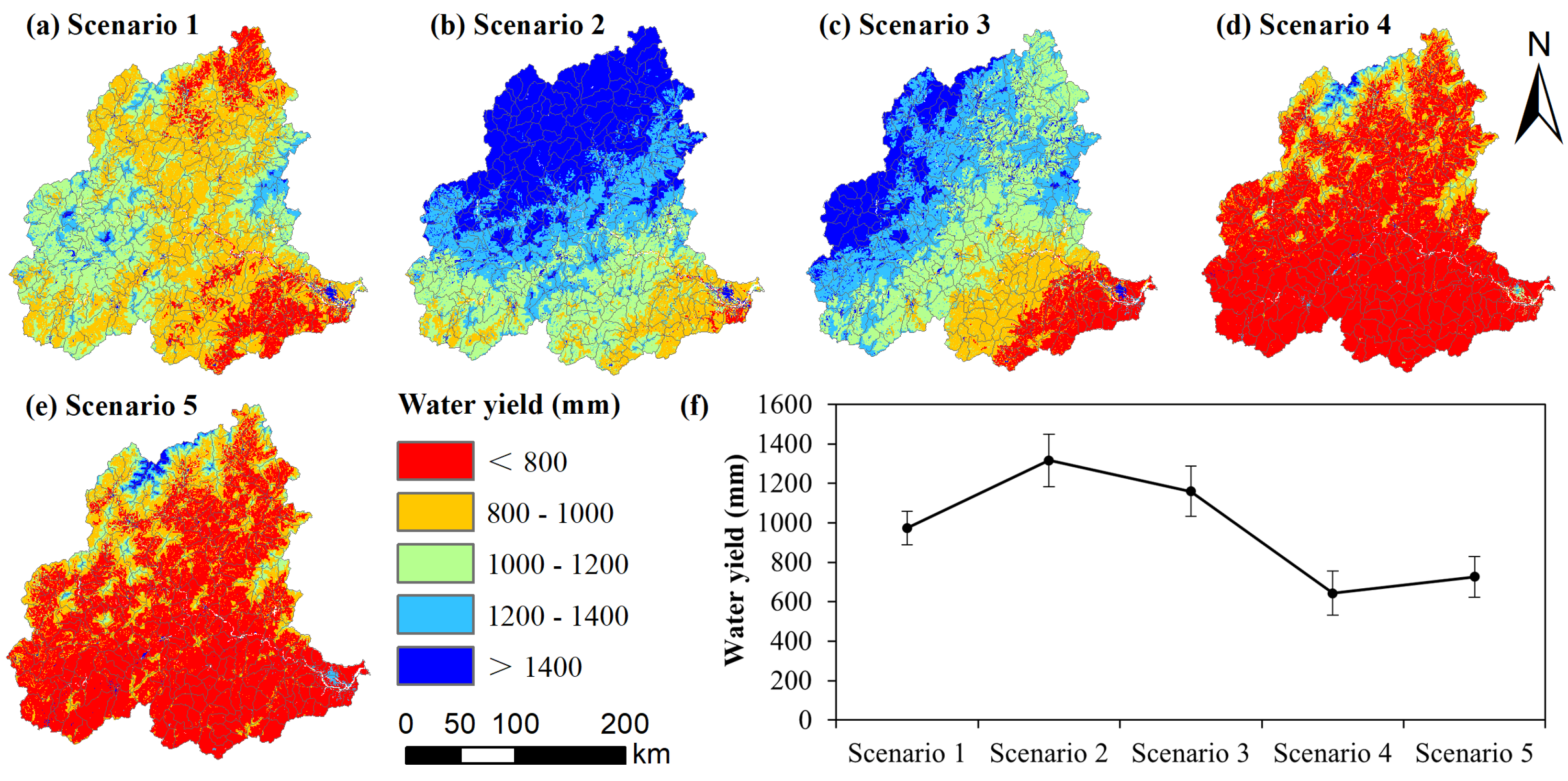
Under the climatic factor change scenarios (Scenarios 1–5), water yield fluctuated significantly (Figure 5), and its spatial pattern was closely consistent with the precipitation distribution of the corresponding years. Compared with the 2000 baseline: water yield increased by 12.83 mm, 355.51 mm, and 199.03 mm in Scenarios 1–3 (using 2005, 2010, and 2015 climate data, respectively); it decreased by 318.18 mm and 233.74 mm in Scenarios 4–5 (using 2020 and 2023 climate data, respectively).
Figure 5.
Simulated water yield under climate-only change scenarios. (a–e) represent the spatial distribution for Scenario 1, Scenario 2, Scenario 3, Scenario 4, and Scenario 5, respectively; (f) represents the line graph with error bars. In each scenario, land use is fixed at the 2000 condition, while climatic factors are replaced with data from 2005, 2010, 2015, 2020, and 2023, respectively.
As expected from the InVEST model structure—where water yield is calculated as precipitation minus evapotranspiration—the spatial patterns under climate-only scenarios (Scenarios 1–5) closely resemble the actual water yield distributions of the corresponding years. This strong precipitation signal is not a novel finding per se, but rather a model-structure-driven baseline against which the additional influences of land use and their interactions are quantified.
3.3.2. Impact of Land Use Change
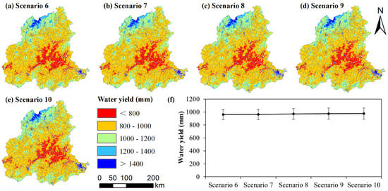
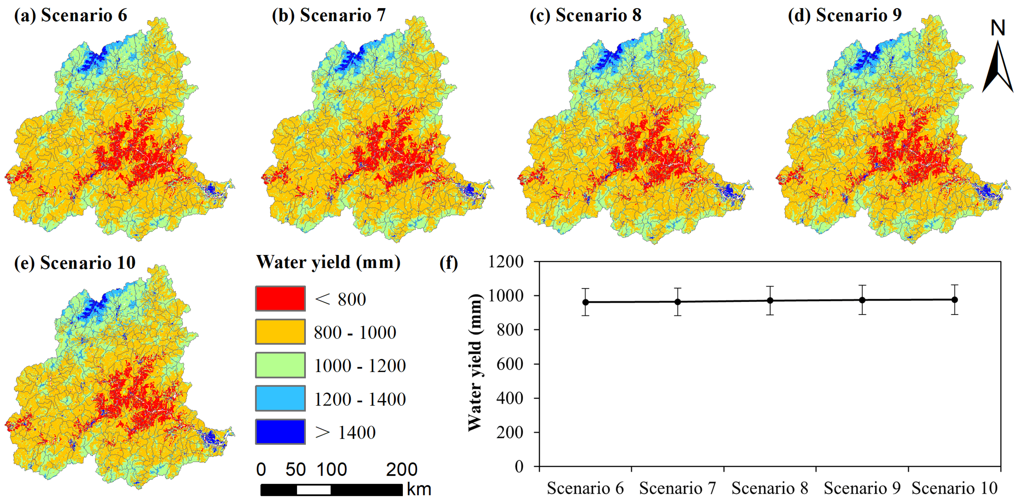
Under the land use change scenarios (Scenarios 6–10), the magnitude of water yield change was relatively small but showed a steady increasing trend (Figure 6). The spatial pattern remained consistent with the 2000 precipitation distribution. Compared with the baseline, the increases in water yield were 1.92 mm (2005), 3.50 mm (2010), 10.56 mm (2015), 14.39 mm (2020), and 15.86 mm (2023) in sequence.
Figure 6.
Simulated water yield under land-use-only change scenarios. (a–e) represent the spatial distribution for Scenario 6, Scenario 7, Scenario 8, Scenario 9, and Scenario 10, respectively; (f) represents the line graph with error bars. In each scenario, climatic factors are fixed at the 2000 condition, while land use data are replaced with maps from 2005, 2010, 2015, 2020, and 2023, respectively.
The small magnitude of water yield change under land-use-only scenarios (Scenarios 6–10) is consistent with the InVEST model structure, where land use influences water yield primarily through the evapotranspiration coefficient (Kc) and root depth, which have weaker effects than precipitation. Therefore, the absolute values of these changes (1.92–15.86 mm) are less informative than their temporal trend and their role in nonlinear interactions. The steady increase from 2005 to 2023 reflects cumulative land use transitions—particularly urban expansion and agricultural intensification—that gradually alter the basin’s hydrological response. More importantly, when these land use changes co-occur with climate variability, they produce substantial nonlinear interaction effects. This indicates that land use, despite its weak direct signal, significantly modulates the system’s sensitivity to climate.
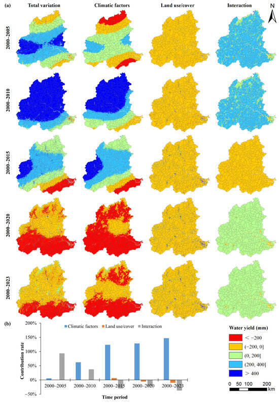
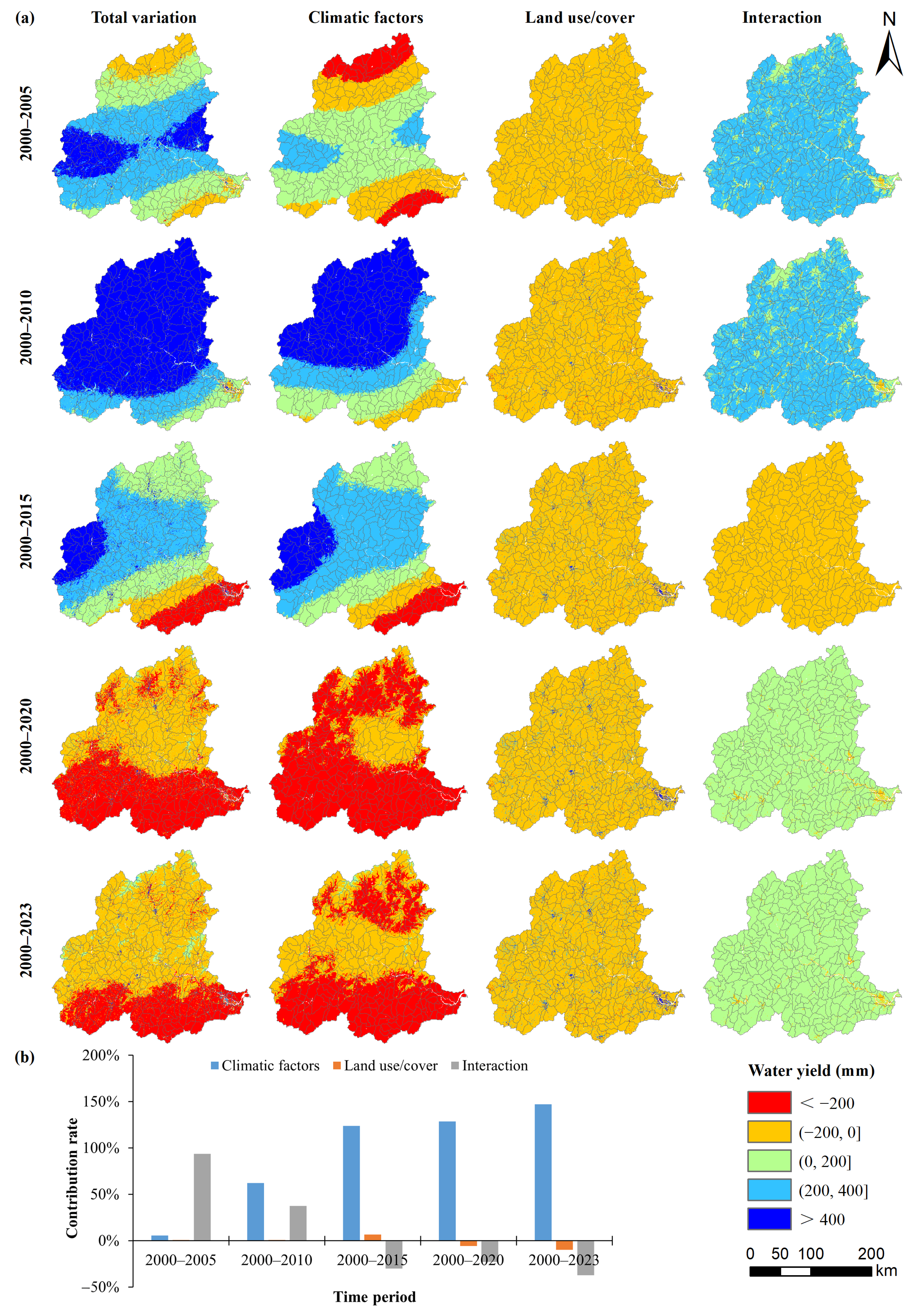
3.3.3. Contribution Rate Decomposition
Changes in climatic factors dominated the spatiotemporal evolution of water yield, with an average contribution rate of 93.43% (Figure 7). Land use change had an average contribution rate of −1.56%, indicating a slight inhibitory effect. The average contribution rate of their interaction was 8.13%. As the time interval extended, the contribution rate of climatic factors continued to rise, increasing from 5.53% (5-year interval) to 147.13% (23-year interval). The specific contributions for each period are as follows: 2000–2005: climatic factors 5.53%, land use 0.83%, interaction 93.64%; 2000–2010: 62.12%, 0.61%, 37.27%; 2000–2015: 123.65%, 6.56%, −30.21%; 2000–2020: 128.72%, −5.82%, −22.90%; 2000–2023: 147.13%, −9.98%, −37.14%. It should be noted that these contribution rates are relative measures derived from the specific baseline year (2000) and scenario design. They represent the proportional attribution of observed changes under the assumption that climate and land use are the only varying factors, and should not be interpreted as absolute physical shares of water yield.
Figure 7.
Decomposition of water yield changes and contribution rates. (a) Time series of basin-average water yield under the baseline (2000), climate-only, land-use-only, and combined scenarios. (b) Contribution rates of climatic factors, land use change, and their nonlinear interaction to the total water yield change relative to the 2000 baseline.
Notably, the interactive contribution rate shifted from strongly positive (93.64%) during 2000–2005 to increasingly negative values thereafter (e.g., −37.14% during 2000–2023). This shift suggests a transition from synergistic to antagonistic nonlinear interactions between climate and land use. In the early 2000s, ecological restoration efforts (e.g., afforestation) likely enhanced the infiltration and retention capacity of the basin, amplifying the runoff response to increased precipitation. However, as urban expansion accelerated and forest cover matured, the marginal hydrological regulation capacity may have diminished, while impervious surfaces reduced infiltration and accelerated surface runoff, thereby weakening the efficiency of precipitation-to-water-yield conversion under drier conditions. This interpretation is supported by the declining explanatory power of precipitation alone in later periods and the strengthened interaction between forest and precipitation (q > 95%), indicating that land use no longer acts independently but modulates climate effectiveness.
3.4. Driver Detection
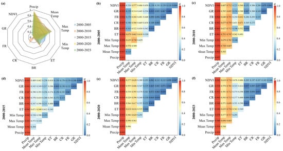
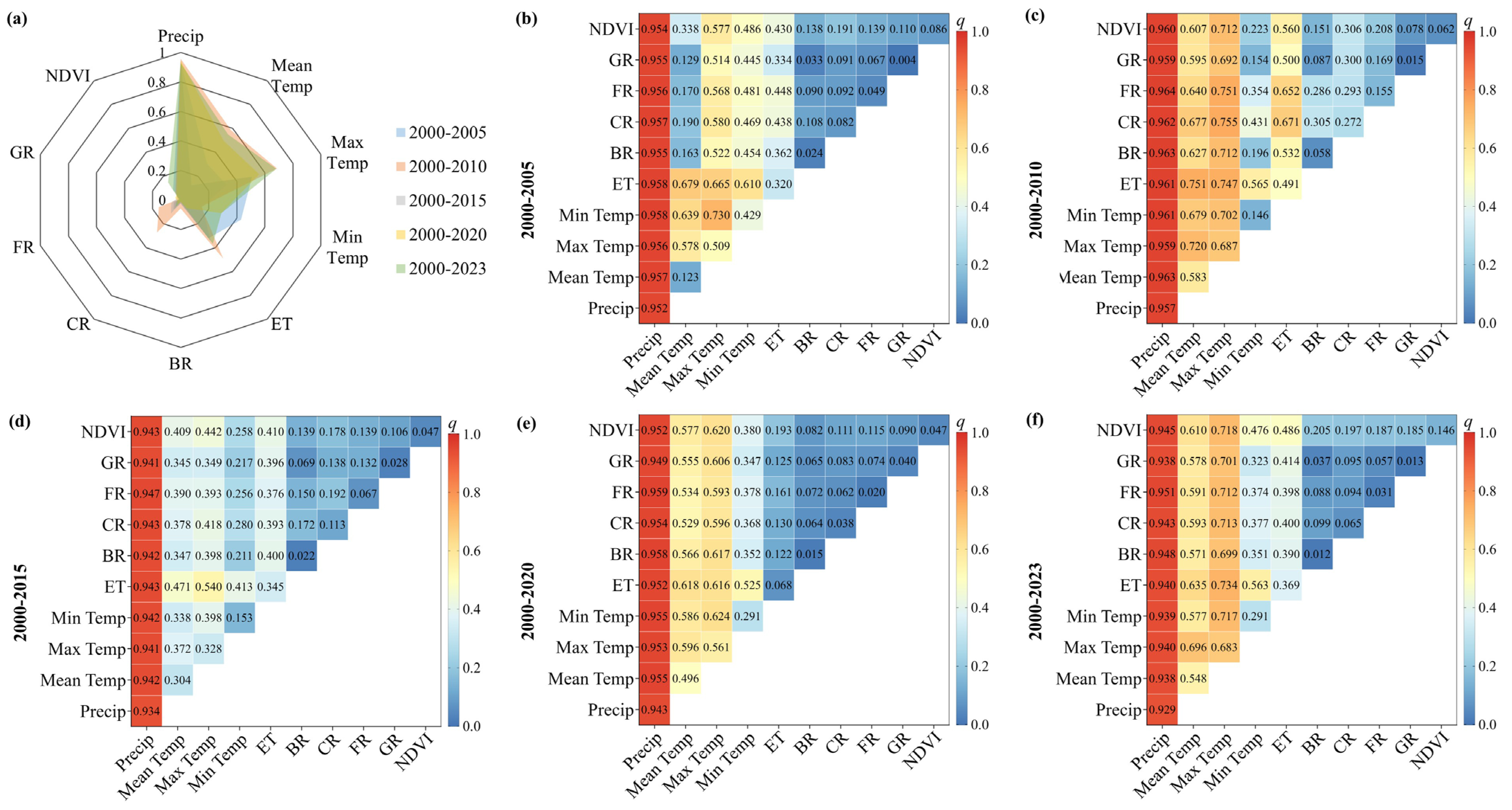
Among climatic factors, precipitation exhibited the strongest explanatory power for the spatial differentiation of water yield (average q = 94%) (Figure 8), followed by maximum temperature (55%), while minimum temperature had the weakest explanatory power (26%). Among land use factors, the proportion of cropland had the greatest explanatory power (11%), followed by NDVI (8%), with grassland having the least (2%). The relatively lower explanatory power of PAWC is attributed to the relatively homogeneous soil texture and moderate topographic variability across the basin, which limits its capacity to explain spatial contrasts in water yield compared to the strong precipitation gradient.
Figure 8.
Explanatory power of individual factors and their interactions on the spatial differentiation of water yield, derived from the Geographical Detector model. (a) Single-factor q-values for climatic factors and land use factors. (b–f) Interactive q-values for selected factor pairs.
The interaction between precipitation and other factors dominated the spatiotemporal evolution of water yield. Across different periods: the interaction between precipitation and minimum temperature/actual evapotranspiration had the highest explanatory power in 2000–2005 (95.8%); the interaction between precipitation and forest consistently showed the highest explanatory power in 2000–2010 (96.4%), 2000–2015 (94.7%), 2000–2020 (95.9%), and 2000–2023 (95.1%); the interaction between grassland and construction land consistently had the lowest explanatory power across all periods (3.3–8.7%), indicating its minor influence on the spatial pattern of water yield.
4. Discussion
4.1. Model Calibration and Applicability
Through systematic parameter calibration, this study identifies Z = 6 as the optimal seasonal parameter for the InVEST Water Yield model in the MRB, reducing the average relative error of simulated water yield to just 1.04%. This optimal parameter value reflects the integrated influence of seasonal precipitation distribution and underlying surface characteristics on hydrological processes within the basin. The high post-calibration accuracy (average 98.96%) validates the applicability of the InVEST model—grounded in Budyko hydro-climatic coupling theory—at the basin scale in humid regions, establishing a reliable foundation for subsequent scenario analysis. Sensitivity analysis of the Z parameter further revealed its substantial impact on simulation results, underscoring that appropriate localized calibration is an essential prerequisite for ensuring assessment accuracy [24].
We acknowledge certain limitations in the validation approach. Due to the lack of spatially distributed or seasonal observations, validation was performed only at the basin scale using annual runoff depth. While the high NSE and coefficient of determination confirm the model’s ability to reproduce annual totals and interannual variability, its performance at sub-basin scales or seasonal time steps remains untested. Future studies should prioritize the collection of spatially distributed hydrological data to enable more rigorous, multi-scale validation.
It is also important to note the implications of data resampling. Climate forcing data were resampled from their original 1000 m resolution to 30 m to align with high-resolution land use inputs. While this procedure ensures spatial consistency, it does not introduce new information at the sub-kilometer scale; actual climatic variability below 1000 m is not captured. Consequently, the fine-scale (30 m) heterogeneity in simulated water yield is predominantly driven by land use and topographic attributes, which vary at higher spatial frequency. This interpretation aligns with the scenario analysis results, where land use change—despite its low average contribution to total water yield—produced detectable spatial differences over time.
Finally, it is important to acknowledge the structural limitations of the modeling approach. The InVEST Water Yield model, while widely used and computationally efficient, simplifies hydrological processes by assuming steady-state conditions and neglecting subsurface flow pathways, groundwater interactions, and temporal lags between precipitation and runoff. These structural simplifications introduce uncertainty, particularly in capturing intra-annual dynamics and baseflow contributions. The high calibration accuracy achieved in this study (NSE = 0.9978) suggests that these simplifications are acceptable for annual-scale analysis in this humid basin; however, process-based models (e.g., SWAT, MIKE SHE) may be necessary for more detailed mechanistic understanding and for applications requiring sub-annual or event-scale resolution.
4.2. Dominant Influence of Climatic Factors
This study confirms that climatic factors are the predominant drivers of spatiotemporal water yield evolution in the MRB, with an average contribution rate of 93.43%. This finding is robustly corroborated by the Geographical Detector results: precipitation alone explains 94% (p < 0.01) of the spatial differentiation in water yield, emphatically underscoring the central role of the precipitation-runoff process in humid basins.
The analysis further reveals a hierarchical influence among temperature components. Maximum temperature exhibits substantial explanatory power (55%, p < 0.05), indicating that extreme high temperatures suppress water yield by enhancing potential evapotranspiration [27]. In contrast, minimum temperature contributes relatively weakly (26%), suggesting that nocturnal low temperatures exert limited influence on daytime hydrological processes. This temperature hierarchy has important implications for understanding how different facets of climate change may affect water resources.
Notably, the contribution rate of climatic factors increases markedly with extended time intervals—from 5.53% over five years to 147.13% over the full 23-year period. This progressive increase highlights the profound cumulative impact of long-term climate change on water resource systems, which ultimately far exceeds the effects of human activities such as land use change [28,29,30]. The interpretation of rates exceeding 100%, as discussed in Section 2.3.3, reflects the non-additive nature of climate–land interactions rather than a physical impossibility.
The influence of climate extremes on water yield is also noteworthy. The exceptionally high water yield in 2010 coincided with extreme precipitation events associated with typhoons, while the low yield in 2020 reflected a prolonged dry period. These extremes amplify the nonlinearity of hydrological responses and underscore the need for climate-resilient management strategies that account for increased variability under future climate scenarios.
4.3. Differential Regulation by Land Use and Its Nonlinear Interactions
4.3.1. Direct Versus Interactive Effects of Land Use
Although the direct contribution of land use change to water yield evolution is minimal (average −1.56%), indicating a slight overall inhibitory effect, its influence varies distinctly across land use types. Factor detection results reveal that cropland proportion exhibits the greatest explanatory power among land use factors (11%), attributable to its direct effects on surface runoff, irrigation, and infiltration processes [31,32]. NDVI, as an indicator of vegetation cover, explains 8% of spatial variation, reflecting the hydrological regulation function of ecosystems [33].
More significantly, interaction detection demonstrates prevalent nonlinear enhancement effects between climatic factors and land use, with an average interactive contribution rate of 8.13%. Notably, the interaction between precipitation and forest land consistently exhibits exceptionally strong explanatory power across all periods (up to 96.4%), highlighting the critical role of forest cover in regulating precipitation redistribution through enhanced water conservation and runoff regulation capacities [34,35,36]. In contrast, the interaction between construction land and grassland is consistently weakest (3.3–8.7%), suggesting that urban expansion may simplify water yield processes by altering surface permeability [18,37].
These findings indicate that assessing only the independent contribution of land use would severely underestimate its actual impact. The nonlinear effects arising from complex interactions—whether synergistic or antagonistic—with climatic factors are indispensable mechanisms shaping the spatial pattern of water yield.
4.3.2. The Role of Soil Properties
We acknowledge that soil properties, particularly PAWC, are physically embedded in the InVEST model structure. However, their spatial explanatory power in this basin is secondary to precipitation, as the MRB exhibits relatively uniform soil texture classes (loam to sandy loam) and consistent soil depth. This does not diminish the importance of soils in hydrological processes but rather reflects that, under current conditions, the precipitation gradient serves as the first-order control on spatial variation in water yield. In basins with stronger soil heterogeneity, PAWC may emerge as a more influential factor.
4.3.3. Reconciling Interaction Metrics
A critical conceptual distinction must be made between the two interaction metrics employed in this study, as they capture complementary yet distinct dimensions of nonlinearity: (1) The scenario-derived interaction contribution (Ri) represents the non-additive effect—the portion of water yield change that cannot be explained by the linear sum of independent climate and land use effects. (2) The Geographical Detector interaction (q(X1 ∩ X2)) quantifies spatial synergism—the extent to which two factors jointly explain the spatial heterogeneity of water yield beyond their individual contributions.
These two metrics are physically connected through shared biogeophysical feedback mechanisms. For example, the persistently high q-value for precipitation–forest interaction (up to 96.4%) indicates that forests exert spatially varying control on infiltration, evapotranspiration, and runoff generation. When both precipitation and forest cover change over time, this spatial coupling translates into a nonlinear temporal response—amplifying water yield in wet periods (synergistic) or dampening it under dry conditions (antagonistic).
Thus, the negative Ri values observed in later periods (e.g., −37.14% during 2000–2023) reflect the temporal manifestation of the same spatial mechanism: the hydrological regulation capacity of forests, while strong, can become saturated or offset by urbanization, leading to diminished precipitation sensitivity. This reconciliation strengthens the physical basis for integrating climate–land governance.
4.3.4. Cautions in Interpreting Interaction Results
While the Geographical Detector provides a robust non-parametric measure of spatial association, its interaction results warrant careful interpretation. The high q-values for precipitation–forest interactions (up to 96.4%) indicate strong spatial covariance, but do not necessarily imply causal dominance in a physical sense—forests tend to be located in high-precipitation areas, which can inflate statistical associations.
Alternative spatial methods such as geographically weighted regression (GWR) or multiscale geographically weighted regression (MGWR) could provide complementary insights into spatial non-stationarity of driver effects. However, these methods require different assumptions (e.g., linearity in local models) and are not directly comparable to the factor interaction framework of the Geographical Detector. Therefore, we interpret our results as evidence of strong spatial coupling between precipitation and forest cover—physically consistent with known hydrological feedback mechanisms—rather than as proof of exclusive causal dominance.
4.3.5. Model Limitations and Future Directions
It is important to acknowledge that the InVEST model simulates natural water yield (precipitation minus evapotranspiration) and does not account for anthropogenic water withdrawals, reservoir regulation, or groundwater extraction. In the lower reaches of the MRB, where intensive agriculture and urban water use occur, actual available water resources may be substantially lower than simulated water yield. Future studies should integrate socio-hydrological models to quantify the gap between natural supply and human demand, providing a more complete picture of water resource availability under changing environmental conditions.
4.4. Implications for Integrated Watershed Management
First, water resource planning must prioritize climate change adaptation by establishing dynamic assessment and early warning mechanisms grounded in long-term climate predictions. Given the increasing spatiotemporal variability of precipitation documented in this study—exemplified by the contrast between the extreme wet year of 2010 and the dry year of 2020—such proactive systems are essential for anticipating and mitigating hydrological extremes. The dominant contribution of climatic factors (93.43%) to water yield evolution underscores that climate variability is the primary driver of water resource fluctuations, and management strategies must be designed with this reality as their foundation.
Second, differentiated land use optimization strategies should be implemented across the basin, tailored to the hydrological functions and vulnerabilities of specific zones. (1) Upper reaches and water source areas: Given the exceptionally strong precipitation–forest interaction (q > 95%), protecting and improving the quality of forest cover in these regions should be prioritized to maximize hydrological regulation benefits. Based on our findings, maintaining forest coverage above 70% in the upper reaches of the MRB can significantly enhance the basin’s hydrological regulation capacity and reduce water yield volatility under extreme climatic conditions. (2) Agricultural areas: In cropland-dominated zones, promoting water-saving irrigation and conservation tillage practices can reduce water consumption while maintaining agricultural productivity [38,39]. The relatively higher explanatory power of cropland proportion (11%) among land use factors suggests that agricultural management decisions have detectable impacts on water yield patterns. (3) Urban and peri-urban areas: Strict regulation of uncontrolled urban expansion is necessary, coupled with enhanced construction of sponge city facilities to improve the detention and infiltration capacity of underlying surfaces [40,41]. The weak interactions between construction land and other factors (3.3–8.7%) suggest that current urbanization patterns may simplify hydrological processes, underscoring the need for green infrastructure that restores some degree of hydrological complexity.
Third, systemic governance based on climate–land nonlinear interactions must be advanced. Water resource management policies should abandon single-factor thinking and explicitly emphasize the interactive effects between climatic conditions and land use types. For instance, in areas with high precipitation variability, land types with high vegetation cover should be prioritized to buffer runoff fluctuations. This represents a paradigm shift from traditional approaches that treat climate and land use as independent management domains toward integrated strategies that recognize their fundamental interdependence.
The consistently high explanatory power of the precipitation–forest interaction (q > 95%) provides a strong evidence base for targeted policy interventions. We recommend prioritizing forest-based climate adaptation strategies in sub-basins characterized by high interannual precipitation variability. Specifically, maintaining forest coverage above 70% in the upper reaches of the MRB can significantly enhance the basin’s hydrological regulation capacity and reduce water yield volatility under extreme climatic conditions. This recommendation is directly supported by the nonlinear interaction effects quantified in this study and represents a concrete application of climate–land integrated management principles.
Finally, the methodological framework and management principles developed here are transferable to other basins facing similar environmental changes. The decoupling-parsing paradigm—combining process-based modeling, scenario analysis, and spatial interaction detection—can help identify dominant drivers and their nonlinear interactions in diverse hydrological settings, supporting the development of locally tailored, climate-resilient management strategies worldwide.
5. Conclusions
This study integrates the InVEST model, scenario analysis, and Geographical Detector to evaluate spatiotemporal water yield evolution in the MRB (2000–2023) and quantitatively decouple the contributions of climatic factors, land use change, and their interactions. The main conclusions are:
Climatic factors overwhelmingly control water yield evolution, with an average contribution of 93.43% that increases with longer time intervals. Precipitation decisively explains spatial water yield patterns (q = 94%), while maximum temperature exerts a significant inhibitory effect through enhanced evapotranspiration.
Although the direct contribution of land use change is minimal (−1.56%), its influence operates primarily through nonlinear interactions with climate (average 8.13%). The precipitation–forest interaction exhibits exceptionally strong explanatory power (q up to 96.4%), highlighting forests’ critical role in regulating hydrological processes. In contrast, built-up land interactions are consistently weak, suggesting urbanization simplifies hydrological responses.
The coupled scenario-detector framework enables precise decoupling of driver contributions and reveals the underlying interaction mechanisms, offering a transferable paradigm for watershed management. Key limitations include residual-based interaction estimates, spatial covariance versus causality, basin-scale validation only, and model structural simplifications. Future work should integrate process-based models, incorporate socio-economic data, extend to seasonal/event timescales, and apply the framework across diverse basins to test generalizability.
Water resource management must shift toward systemic governance based on coupled climate–land relationships, recognizing that interactive effects fundamentally shape hydrological responses. This study provides both the analytical tools and empirical evidence to support this paradigm shift in an era of rapid environmental change.
Author Contributions
Conceptualization, P.D. and Y.T.; methodology, B.S.; software, B.S.; validation, B.S., J.Z. and Y.F.; formal analysis, P.D.; investigation, B.S.; resources, P.D.; data curation, B.S.; writing—original draft preparation, P.D.; writing—review and editing, P.D.; visualization, P.D.; supervision, P.D. and Y.T.; project administration, P.D.; funding acquisition, P.D. All authors have read and agreed to the published version of the manuscript.
Funding
This research was funded by the Social Science Foundation of Fujian Province, grant number FJ2024C086 and FJ2025C245; the Startup Fund for Advanced Talents of Putian University, grant number 2023012 and the Graduate Research Innovation Project of Putian University, grant number yjs2024023.
Institutional Review Board Statement
Not applicable.
Informed Consent Statement
Not applicable.
Data Availability Statement
The original contributions presented in this study are included in the article. Further inquiries can be directed to the corresponding authors.
Acknowledgments
The authors are very grateful to the editors and reviewers for their generous help in the publication of this paper.
Conflicts of Interest
The authors declare no conflicts of interest.
References
- Damania, R. The economics of water scarcity and variability. Oxford Rev. Econ. Pol. 2020, 36, 24–44. [Google Scholar] [CrossRef] [Scilit]
- Li, J.H.; Zhao, M.D.; Han, Y.P.; Wei, J.H. Analysis of water resource ecological optimization and obstacles based on the water resources-socio-economic-ecological environment model framework—A case study of the core area of the Central Plains urban agglomeration. Front. Ecol. Evol. 2023, 11, 1263601. [Google Scholar] [CrossRef] [Scilit]
- Lu, C.; Sidai, G.; Yangli, L. Discerning changes and drivers of water yield ecosystem service: A case study of Chongqing-Chengdu District, Southwest China. Ecol. Indic. 2024, 160, 111767. [Google Scholar] [CrossRef] [Scilit]
- Yang, X.X.; Gu, X.C.; Zhang, P.; Liu, J.; Zhang, W.J.; Long, A.H. Assessment of the Impacts of Climate and Land Use Changes on Water Yield in the Ebinur Lake Basin. Land 2024, 13, 1324. [Google Scholar] [CrossRef] [Scilit]
- Swain, S.S.; Mishra, A.; Chatterjee, C.; Sahoo, B. Climate-changed versus land-use altered streamflow: A relative contribution assessment using three complementary approaches at a decadal time-spell. J. Hydrol. 2021, 596, 126064. [Google Scholar] [CrossRef] [Scilit]
- Zhan, C.S.; Zeng, S.D.; Jiang, S.S.; Wang, H.X.; Ye, W. An Integrated Approach for Partitioning the Effect of Climate Change and Human Activities on Surface Runoff. Water Resour. Manag. 2014, 28, 3843–3858. [Google Scholar] [CrossRef] [Scilit]
- He, Y.; Qiu, H.J.; Song, J.X.; Zhao, Y.; Zhang, L.M.; Hu, S.; Hu, Y.Y. Quantitative contribution of climate change and human activities to runoff changes in the Bahe River watershed of the Qinling Mountains, China. Sustain. Cities Soc. 2019, 51, 101729. [Google Scholar] [CrossRef] [Scilit]
- Deng, J.; Xiao, J.F.; Ouimette, A.; Zhang, Y.; Sanders-Demott, R.; Frolking, S.; Li, C.S. Improving a Biogeochemical Model to Simulate Surface Energy, Greenhouse Gas Fluxes, and Radiative Forcing for Different Land Use Types in Northeastern United States. Glob. Biogeochem. Cycles 2020, 34, e2019GB006520. [Google Scholar] [CrossRef] [Scilit]
- Wei, B.; Li, Z.W.; Duan, L.X.; Gu, Z.K.; Liu, X.M. Vegetation types and rainfall regimes impact on surface runoff and soil erosion over 10 years in karst hillslopes. CATENA 2023, 232, 107443. [Google Scholar] [CrossRef] [Scilit]
- Saher, R.; Stephen, H.; Ahmad, S. Effect of land use change on summertime surface temperature, albedo, and evapotranspiration in Las Vegas Valley. Urban Clim. 2021, 39, 100966. [Google Scholar] [CrossRef] [Scilit]
- Zhu, Y.X.; Zhang, Y.J.; Li, Y.; Zheng, Z.T.; Zhao, G.; Sun, Y.H.; Gao, J.; Chen, Y.; Zhang, J.S.; Zhang, Y. Human activities further amplify the cooling effect of vegetation greening in Chinese drylands. Agr. For. Meteorol. 2023, 342, 109703. [Google Scholar] [CrossRef] [Scilit]
- Wen, Y.Y.; You, T.G.; Xu, Y.H.; Lin, S.H.; Ning, J.; You, X.M.; Xiao, Y.L. Comprehensive Evaluation of the Level of Water Ecological Civilization Construction in the Min River Basin, China. Sustainability 2022, 14, 15753. [Google Scholar] [CrossRef] [Scilit]
- Wang, S.Z.; Chen, X.W.; Yao, H.X.; Ruan, W.F.; Gu, Z.P.; Li, X.C.; Chen, Y.; Liu, M.B.; Deng, H.J. Separation and spatial variations of typhoon and non-typhoon rainfall at different timescales in typical region of southeast China. Int. J. Climatol. 2024, 44, 4611–4628. [Google Scholar] [CrossRef] [Scilit]
- Zheng, P.; Jin, L.T.; Huang, Y.X.; Pan, W.B. Spatial and Temporal Dynamic Evolution and Correlation of Ecological Quality and Ecosystem Service Value in Fujian Province. Sustainability 2024, 16, 5063. [Google Scholar] [CrossRef] [Scilit]
- Zhang, Y.; Deng, C.; Xu, W.; Zhuang, Y.; Jiang, L.; Jiang, C.; Guan, X.; Wei, J.; Ma, M.; Chen, Y.; et al. Long-term variability of extreme precipitation with WRF model at a complex terrain River Basin. Sci. Rep. 2025, 15, 156. [Google Scholar] [CrossRef] [Scilit]
- Lu, Y.J.; Wang, Y.Y.; Liu, Q.; Chen, X.W.; Zhang, Y.Q.; Gao, L.; Chen, Y.; Liu, M.B.; Deng, H.J. Evapotranspiration Variations of the Minjiang River Basin in Southeastern China from 2000 to 2019. Atmosphere 2022, 13, 562. [Google Scholar] [CrossRef] [Scilit]
- Luo, F.; He, L.; He, Z.W.; Zeng, W.; Wang, Y.C. Evaluation of Coastal Ecological Security Barrier Functions Based on Ecosystem Services: A Case Study of Fujian Province, China. Sustainability 2024, 16, 6787. [Google Scholar] [CrossRef] [Scilit]
- Shrestha, S.; Cui, S.H.; Xu, L.L.; Wang, L.H.; Manandhar, B.; Ding, S.P. Impact of Land Use Change Due to Urbanisation on Surface Runoff Using GIS-Based SCS–CN Method: A Case Study of Xiamen City, China. Land 2021, 10, 839. [Google Scholar] [CrossRef] [Scilit]
- Chen, X.; Lin, S.Y.; Tian, J.; Wang, Y.J.; Ye, Y.X.; Dong, S.N.; Gong, X.L.; Lin, Q.L.; Zhu, L.Y. Simulation study on water yield service flow based on the InVEST-Geoda-Gephi network: A case study on Wuyi Mountains, China. Ecol. Indic. 2024, 159, 111694. [Google Scholar] [CrossRef] [Scilit]
- Geng, K.L.; Chen, X.W.; Zheng, M.L.; Gao, Y.P.; Gu, Z.P.; Yao, H.X. The influence of human activities on rainfall-runoff relationships at different time scales in the Minjiang River Basin. Theor. Appl. Climatol. 2024, 155, 8435–8454. [Google Scholar] [CrossRef] [Scilit]
- Xu, X.; Genovese, P.V.; Zhao, Y.F.; Liu, Y.D.; Woldesemayat, E.M.; Zoure, A.N. Geographical Distribution Characteristics of Ethnic-Minority Villages in Fujian and Their Relationship with Topographic Factors. Sustainability 2022, 14, 7727. [Google Scholar] [CrossRef] [Scilit]
- Xiong, J.N.; Pang, Q.; Fan, C.K.; Cheng, W.M.; Ye, C.C.; Zhao, Y.L.; He, Y.R.; Cao, Y.F. Spatiotemporal Characteristics and Driving Force Analysis of Flash Floods in Fujian Province. ISPRS Int. J. Geo Inf. 2020, 9, 133. [Google Scholar] [CrossRef] [Scilit]
- Wu, Y.J.; Mu, H.L.; Wu, S.-Y.; Xu, Y.; Xu, M.; Wu, H.W.; Clark, R.T.; Gao, C. Changes in mean and extreme homogeneous precipitation in China during 1960–2020. Atmos. Res. 2023, 292, 106891. [Google Scholar] [CrossRef] [Scilit]
- Liu, M.J.; Zhong, J.T.; Xu, S.Y. Simulation of Spatial and Temporal Variations in the Water Yield Function in the Source Area of the Yellow River and an Analysis of Influencing Factors. Sustainability 2024, 16, 8259. [Google Scholar] [CrossRef] [Scilit]
- Xu, M.J.; Feng, Q.; Zhang, S.R.; Lv, M.; Duan, B.L. Ecosystem Services Supply–Demand Matching and Its Driving Factors: A Case Study of the Shanxi Section of the Yellow River Basin, China. Sustainability 2023, 15, 11016. [Google Scholar] [CrossRef] [Scilit]
- Shang, S.W.; Cui, T.T.; Wang, Y.T.; Gao, Q.T.; Liu, Y. Dynamic variation and driving mechanisms of land use change from 1980 to 2020 in the lower reaches of the Yangtze River, China. Front. Environ. Sci. 2024, 11, 1335624. [Google Scholar] [CrossRef] [Scilit]
- Davamani, V.; John, J.E.; Poornachandhra, C.; Gopalakrishnan, B.; Arulmani, S.; Parameswari, E.; Santhosh, A.; Srinivasulu, A.; Lal, A.; Naidu, R. A Critical Review of Climate Change Impacts on Groundwater Resources: A Focus on the Current Status, Future Possibilities, and Role of Simulation Models. Atmosphere 2024, 15, 122. [Google Scholar] [CrossRef] [Scilit]
- Li, Y.L.; He, Y.; Liu, W.Q.; Jia, L.P.; Zhang, Y.R. Evaluation and Prediction of Water Yield Services in Shaanxi Province, China. Forests 2023, 14, 229. [Google Scholar] [CrossRef] [Scilit]
- Wei, P.J.; Chen, S.Y.; Wu, M.H.; Deng, Y.F.; Xu, H.J.; Jia, Y.L.; Liu, F. Using the InVEST Model to Assess the Impacts of Climate and Land Use Changes on Water Yield in the Upstream Regions of the Shule River Basin. Water 2021, 13, 1250. [Google Scholar] [CrossRef] [Scilit]
- Ma, P.; Lyu, S.H.; Diao, Z.Y.; Zheng, Z.R.; He, J.; Su, D.R.; Zhang, J.R. How Does the Water Conservation Function of Hulunbuir Forest–Steppe Ecotone Respond to Climate Change and Land Use Change? Forests 2022, 13, 2039. [Google Scholar] [CrossRef] [Scilit]
- Umukiza, E.; Abagale, F.K.; Adongo, T.A. Characterization of landuse and landcover dynamics and their impact on runoff generation patterns in dam catchments of Northern Ghana. Geocarto Int. 2024, 39, 2335247. [Google Scholar] [CrossRef] [Scilit]
- Deng, C.X.; Li, Y.Q.; Liu, Y.J.; Liu, C.C.; Zhang, G.J. Rice Terraces Enhanced the Hydrological Stability of Small Watershed with LUCC—A Case Study of Xinhua Basin. Water 2024, 16, 712. [Google Scholar] [CrossRef] [Scilit]
- Feng, H.H.; Zou, B.; Luo, J.H. Coverage-dependent amplifiers of vegetation change on global water cycle dynamics. J. Hydrol. 2017, 550, 220–229. [Google Scholar] [CrossRef] [Scilit]
- Chen, S.Y.; Tian, L.; Zhang, B.Q.; Zhang, G.S.; Zhang, F.M.; Yang, K.; Wang, X.J.; Bai, Y.; Pan, B.T. Quantifying the impact of large-scale afforestation on the atmospheric water cycle during rainy season over the Chinese Loess Plateau. J. Hydrol. 2023, 619, 129326. [Google Scholar] [CrossRef] [Scilit]
- Hall, J.; Scholl, M.; Shanley, J.; Matt, S.; Uriarte, M. Forest cover lessens hurricane impacts on peak streamflow. Hydrol. Process. 2024, 38, e15249. [Google Scholar] [CrossRef] [Scilit]
- Gao, Q.; Yu, M. Forest Cover and Locality Regulate Response of Watershed Discharge to Rainfall Variability in Caribbean Region. Forests 2024, 15, 154. [Google Scholar] [CrossRef] [Scilit]
- Huang, S.Z.; Gan, Y.; Chen, N.C.; Wang, C.; Zhang, X.; Li, C.X.; Horton, D.E. Urbanization enhances channel and surface runoff: A quantitative analysis using both physical and empirical models over the Yangtze River basin. J. Hydrol. 2024, 635, 131194. [Google Scholar] [CrossRef] [Scilit]
- Van Meerveld, I.; Seibert, J. Reforestation effects on low flows: Review of public perceptions and scientific evidence. WIREs Water 2024, 12, e1760. [Google Scholar] [CrossRef] [Scilit]
- Torun, E.; Çakmak, B. Evaluation of water efficiency in agriculture: The case of the Konya closed basin. Irrig. Drain. 2024, 73, 1470–1482. [Google Scholar] [CrossRef] [Scilit]
- Han, J.; Wang, C.Q.; Deng, S.H.; Lichtfouse, E. China’s sponge cities alleviate urban flooding and water shortage: A review. Environ. Chem. Lett. 2023, 21, 1297–1314. [Google Scholar] [CrossRef] [Scilit]
- Hao, Y.M.; Wang, X.C.; Gao, Z.Q.; Qin, Z.; Liu, Z.Y. Analysis on the Decay Law of Water Retention of Sponge City Roads under Cyclic Clogging. Water Cycle, 2025; in press. [CrossRef] [Scilit]

Disclaimer/Publisher’s Note: The statements, opinions and data contained in all publications are solely those of the individual author(s) and contributor(s) and not of MDPI and/or the editor(s). MDPI and/or the editor(s) disclaim responsibility for any injury to people or property resulting from any ideas, methods, instructions or products referred to in the content. |
© 2026 by the authors. Licensee MDPI, Basel, Switzerland. This article is an open access article distributed under the terms and conditions of the Creative Commons Attribution (CC BY) license.