Enhancing Sustainable Waste-to-Energy: A Multi-Controlled Variable Prediction Model for Municipal Solid Waste Incineration Using Shared Features and an Improved Fuzzy Neural Network

Abstract

Municipal solid waste incineration (MSWI) is a critical technology for advancing urban sustainability, contributing to improved environmental quality, optimized energy structures, and the circular economy. However, the realization of these sustainability benefits is contingent upon the stable, efficient, and low-emission operation of the incineration process. This operational stability is directly governed by several key variables, such as furnace temperature, main steam flow rate, flue gas oxygen content, and burnout point temperature. The inherent complexity of controlling these interconnected variables necessitates the development of an accurate multi-variable prediction model to ensure both energy recovery efficiency and environmental compliance, which are core pillars of sustainable waste management. Existing studies have often addressed these key controlled variables in isolation, lacking a unified modeling framework. Furthermore, they have not adequately considered how dimensional differences among these variables impact the performance evaluation of predictive models, a critical oversight for ensuring holistic process sustainability. To address these gaps and support the intelligent operation of sustainable waste-to-energy systems, this study proposes a novel multi-controlled variable modeling method based on shared features and an improved fuzzy neural network. Our integrated approach begins by calculating the Pearson correlation coefficient between each manipulated variable and each controlled variable—selected based on expert knowledge—to assess the distinguishability of operating conditions within the current dataset. Subsequently, a correlation threshold, informed by expert knowledge, is applied to identify shared features that influence multiple controlled variables simultaneously. Finally, we enhance the fuzzy neural network by redefining its evaluation criterion to accommodate variable dimensional differences, leading to the development of a robust multi-controlled variable prediction model. This model is designed to provide a more comprehensive and accurate basis for process control, directly contributing to improved energy efficiency and reduced environmental impact. The effectiveness of our proposed model is validated using operational data from an actual MSWI plant, demonstrating its potential to support more sustainable and economically viable waste-to-energy operations.

1. Introduction

According to statistics, the global annual output of municipal solid waste (MSW) is expected to increase from 1.9 billion tons in 2015 to 3.5 billion tons in 2050, a trend driven primarily by population growth, economic expansion, and changing consumption patterns [1,2]. The rapid urbanization and economic development in China has led to a sharp increase in MSW output—averaging over 5% annual growth from 2011 to 2020—reaching a peak of 240 million tons in 2019 [3,4]. According to a report by the United Nations Environment Programme (UNEP), more than 2 billion tons of MSW are produced worldwide every year [5], and approximately 38% of MSW is not properly managed. Improper MSW management contributes to pollution of air, soil, and water, endangering human health and contributing to approximately 400,000 to 1 million deaths annually. Moreover, greenhouse gas emissions from MSW exacerbate climate change [6].

The composition of MSW is influenced by many factors, including lifestyle, geographical location, and climatic conditions [7]. The treatment of municipal solid waste (MSW) is guided by the integrated goals of waste minimization, resource recovery, and environmentally sound disposal [8]. Traditional landfill methods not only occupy significant land resources but also pose long-term risks of soil and groundwater pollution [9]. While composting and recycling methods have great environmental value, they are often limited by factors such as classification purity, treatment cycle, and cost [10,11]. In this context, MSW incineration technology typically yields significant economic benefits due to its high resource recovery rate and substantial volume reduction effect [12]. Globally, grate incinerators have become one of the most widely used MSW treatment technologies because of their large treatment capacity [13], remarkable volume reduction (waste volume can be reduced by up to 90% [14]), and energy recovery ability. It not only achieves complete combustion but also contributes significantly to waste reduction and energy recovery [15].

Since China started the pilot project of “waste-free city” construction in 2018, Shenzhen, Qingdao, and other cities have significantly improved the resource utilization level of MSW and promoted the realization of sustainable development goals through systematic governance means such as intelligent collection and transportation system and industrial coordination [16]. Stable combustion conditions can ensure that the furnace temperature remains above 850 °C, thus effectively decomposing highly toxic pollutants such as dioxin, thereby avoiding secondary pollution [17,18]. At the same time, it can prevent the equipment from being damaged due to temperature fluctuations or localized high temperatures, prolong the life of core components, and reduce the maintenance cost. In addition, consistent thermal energy output is the key to ensuring the power generation efficiency and the smooth operation of the power grid [19], which contributes to improving the controllability and operation economy of MSW, and ultimately achieving the unification of environmental, social, and economic benefits [20]. However, an unstable MSW process can cause secondary contamination and reduce energy recovery efficiency [21]. Therefore, it is of great significance to study the controlled variable modeling of the MSWI process. The traditional mechanistic model is based on the conservation of mass, energy, momentum, and chemical reaction dynamics, and describes the system’s internal physical–chemical processes using differential algebraic equations [22]. Many parameters have clear physical significance, clear structure, and strong explanation, which is convenient for analyzing the steady, dynamic, and security boundaries. In short, the advantages of the traditional mechanism model are reliable extrapolation, adjustable parameters, and conformity with engineering specifications. The disadvantage is that the modeling period is long, a lot of assumptions and calibrations are needed, and the adaptability to complex boundaries and nonlinear coupling is poor. Obviously, this is difficult to apply to complex and changeable MSWI processes. The model based on the four-stage mechanism of “drying–pyrolysis–combustion–burnout” in [23] can clearly predict the furnace state, but it is difficult to be practical because of its complex modeling, high calculation cost, and poor generalization ability.

The data-driven model directly uses the collected high-dimensional process data, extracts the system behavior pattern through artificial intelligence (AI) algorithms, and establishes the input–output mapping. For example, reference [24] provides a systematic review of the latest advances in data-driven approaches for combustion process modeling, operational state monitoring, and pollutant emission prediction, offering strong theoretical grounding and practical evidence to establish data-driven methods as one of the preferred modeling solutions for municipal solid waste incineration (MSWI) processes. By integrating a Tikhonov regularization decision tree and single-neuron PID controller, the intelligent optimization control of MSWI process is achieved [25], which reduces pollutant emission and improves combustion efficiency. For MSW processes, it is very important to build a data-driven multi-controlled variable model, which typically involves feature selection and model development.

When constructing the multivariate prediction model of the MSWI process, the complex linear and nonlinear correlations between process variables must be addressed. To accurately identify the key features related to different controlled variables (such as furnace temperature and oxygen content in flue gas), Pearson correlation coefficient (PCC) and mutual information (MI) are commonly used for comprehensive analysis. The research shows that PCC can effectively quantify the linear correlation degree between variables [26]. For example, according to the PCC analysis, there may be a strong linear relationship between the volume of primary air and the furnace temperature [27]. MI can capture the generalized statistical dependence among variables, including nonlinear relationships [28]. For example, the complex nonlinear relationship between the calorific value fluctuations of MSW entering the furnace and the concentration of flue gas pollutants can be effectively identified by MI [29]. Through the comprehensive application of PCC and MI analysis, the research shows that some characteristics (such as “primary air volume”) may be strongly correlated with a single controlled variable (such as “furnace temperature”), and another part of the characteristics (such as “steam flow” or “total feed”) may exhibit significant correlation with multiple controlled variables (such as “furnace temperature” and “power generation”) at the same time [30]. A deep discussion on how to identify key process variables affecting multiple controlled variables using data-driven methods in multi-variable control systems and analyze the key impact of these variables on control system performance and decoupling design are made in [31]. It is very important to identify these shared features, because they are usually the key factor of coupling and interference between different control loops. In the subsequent design of collaborative control strategy, accurate modeling and decoupling control of these shared features is the key to improving the control quality of the whole system.

For model construction, typical algorithms include fuzzy neural network (FNN), LSTM, random forest, among others. Compared with the mechanistic model, its advantages include the ability to approximate complex nonlinear, time-varying, and coupled relationships without complete physical knowledge. Additionally, the development cycle is shorter, and scalability is stronger [32]. Currently, the existing research on modeling controlled variables of MSWI process are as follows. A furnace temperature prediction model integrates slow feature analysis with a sparse random configuration network [33]. Qiao et al. proposed a novel algorithm integrating weighted principal component analysis (WPCA) and an improved long short-term memory (ILSTM) network for accurate prediction of oxygen content in municipal solid waste incineration flue gas [34]. A deep learning model incorporating a multi-universe optimization algorithm was developed to predict key parameters [35], including furnace temperature and flue gas oxygen concentration. However, the inherent complexity of the MSW process presents a significant challenge. It is characterized by multi-phase and multi-field coupling, nonlinear time-varying dynamics, and significant pollution risks. These issues, compounded by unstable feed composition, unpredictable reaction mechanisms, difficulties in real-time monitoring of key parameters, and strong coupling control, necessitate a holistic, system-wide collaborative optimization strategy [36]. Addressing the modeling problem of multiple-input multiple-output (MIMO) controlled variables in the MSWI process, a modeling method based on T-S fuzzy neural network (TSFNN)” was proposed [37]. This method lays a foundation for subsequent optimal control. However, it does not consider additional controlled variables, nor does it evaluate the performance of different controlled variables due to dimensional differences.

To address the modeling challenges of multiple controlled variables in the municipal solid waste incineration (MSWI) process, this study proposes a novel multi-controlled variable modeling method based on shared feature identification and an improved fuzzy neural network (Improved FNN). Firstly, building upon domain expert experience, the Pearson correlation coefficient is calculated between multiple manipulated variables and each controlled variable to quantitatively evaluate the variation under the operating conditions represented by the current modeling data. Subsequently, a correlation threshold is established based on expert knowledge to identify the shared features that simultaneously influence multiple controlled variables. Furthermore, the fuzzy neural network is enhanced by redefining its performance index to better capture the underlying process dynamics, thereby constructing a multi-controlled variable prediction model. Finally, the proposed method is validated using actual data from an MSWI power plant. The experimental results demonstrate that the Improved FNN exhibits superior prediction accuracy and robustness across multiple datasets, particularly in terms of the coefficient of determination (R²) and relative root mean square error (RRMSE), providing an effective solution for complex industrial process modeling.

2. Materials and Methods

2.1. Materials

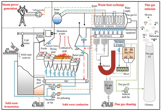
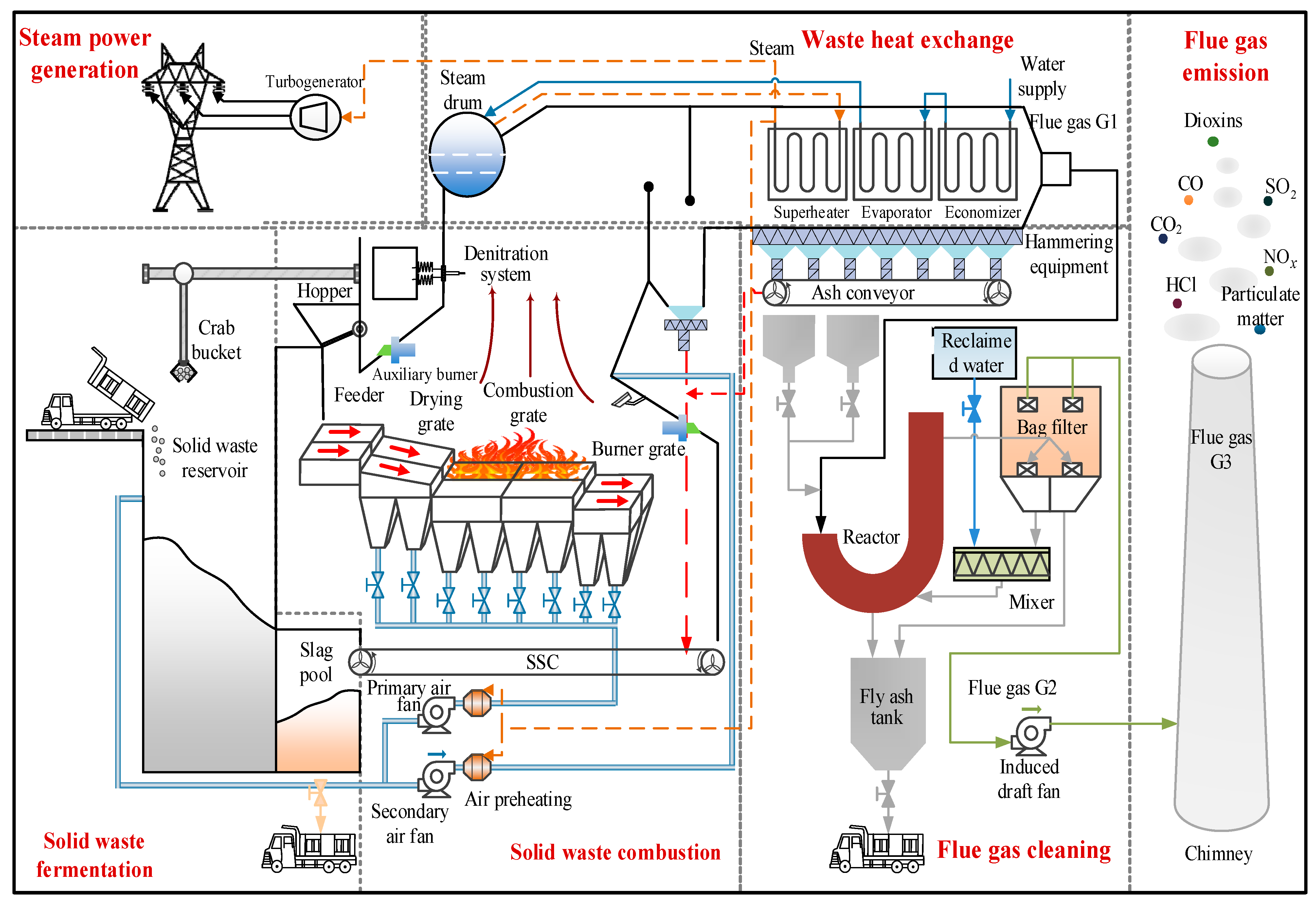
The process flow of typical MSWI process is shown in Figure 1.

Figure 1. Schematic diagram of the MSWI process flow.

As depicted in Figure 1, the municipal solid waste incineration (MSWI) process is based on a grate furnace and comprises several subsystems: solid waste fermentation, solid waste combustion, waste heat recovery, flue gas cleaning, flue gas emission, and others. The process flow is described as follows: municipal solid waste (MSW) is transported to the plant by sanitation vehicles, weighed on the weighbridge, and then discharged into a sealed storage pit. The MSW is fermented and dehydrated in the pit for 5 to 7 days, which reduces its moisture content and increases its calorific value. The fermented MSW is subsequently transferred to the hopper by a bridge crane. The feeder evenly pushes the MSW into the moving grate, where it sequentially passes through the drying section (200–300 °C), the combustion section (850–1050 °C), and the burnout section (600–800 °C). Primary air is supplied from the grate bottom through the fuel bed to provide oxygen, while secondary air is injected tangentially from the furnace sidewalls to enhance turbulence and combustion efficiency.

The combustion process is manually controlled by experienced operators based on various parameters, such as temperature, oxygen content, and steam parameters, to ensure that the residence time of flue gas is maintained at ≥2 s at 850 °C. The ash is discharged via a water-cooled slag catcher and subsequently recycled after magnetic separation. The high-temperature flue gas (above 850 °C) is drawn into the waste heat boiler through the induced draft fan. It flows sequentially through the superheater, evaporator, and economizer, undergoing cascading heat exchange with water in the steam drum to generate superheated steam at a pressure of 4.0–6.5 MPa and a temperature of 400–450 °C, which drives the steam turbine generator set for energy recovery. Meanwhile, the flue gas temperature drops to below 200 °C.

The furnace temperature and flue gas oxygen content are crucial control variables in the MSWI process, collectively determining the combustion quality of the MSW. The main steam flow rate and burnout temperature serve as final indicators of this quality control, reflecting combustion quality in terms of both energy output and residue characteristics. Therefore, an efficient control system must prioritize direct control of primary variables while closely monitoring and optimizing secondary variables. This approach ensures the safe, environmentally friendly, and economically efficient operation of the entire process. Consequently, predictive modeling of these controlled variables is essential for optimizing and maintaining operational performance.

The selected 11 manipulated variables based on expert experience and their ranges used in this article are shown in Table 1.

Table 1. Manipulated variables and their value range.

No.	Name	Range	Unit	Remarks
1	Primary air temperature	[183.4191, 177.2022]	°C	Has the strongest influence on steam flow and furnace temperature and is the primary means to improve combustion efficiency.
2	Total amount of primary air	[58.7867, 74.014]	kNm3/h	Is strongly related to two key indexes and is a direct variable controlling the combustion intensity.
3	Primary wind pressure	[2.0737, 2.8546]	kPa	Ensuring the power of primary air supply is strongly related to steam flow.
4	Air volume in drying section	[10.2630, 14.6249]	kNm3/h	Has the highest correlation with burnout point and is specially used to optimize the combustion end point and ensure burnout.
5	Combustion 1st stage air volume	[27.3574, 37.5719]	kNm3/h	Is directly related to the furnace temperature and is used for accurate air distribution in the main combustion zone.
6	Combustion second stage air volume	[10.8283, 16.5512]	kNm3/h	On the basis of the first stage of combustion, fine adjustment is carried out to ensure that the fuel can be fully burned in the latter stage of the main combustion zone, and at the same time, the temperature of the furnace can be prevented from falling due to excessive air distribution.
7	Burnout section air volume	[5.0809, 8.9791]	kNm3/h	The air volume in the burnout section is mainly used to adjust the burnout point temperature and promote the secondary combustion of unburned materials in fly ash, and the burnout point temperature is the most important factor.
8	Secondary air temperature	[22.5949, 23.8812]	°C	Affects the temperature of combustion zone and has a good correlation with steam flow.
9	Secondary air volume	[0, 10.9899]	kNm3/h	Gives consideration to the control of steam flow and burnout point, and realizes the ratio of burnout air.
10	Feeding speed	[20.53, 75]	t/h	The fundamental control means of boiler load, all air volume adjustments need to match it.
11	Grate speed in drying section	[20, 38.75]	mm/s	Is very important for combustion stability to control the most effective variable of oxygen content in flue gas and adjust the drying and moving speed of fuel at the same time.

2.2. Methods

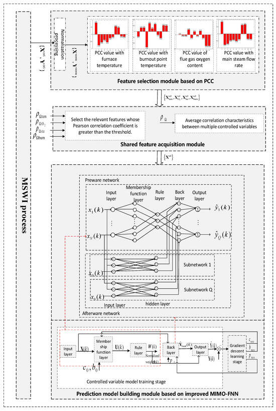
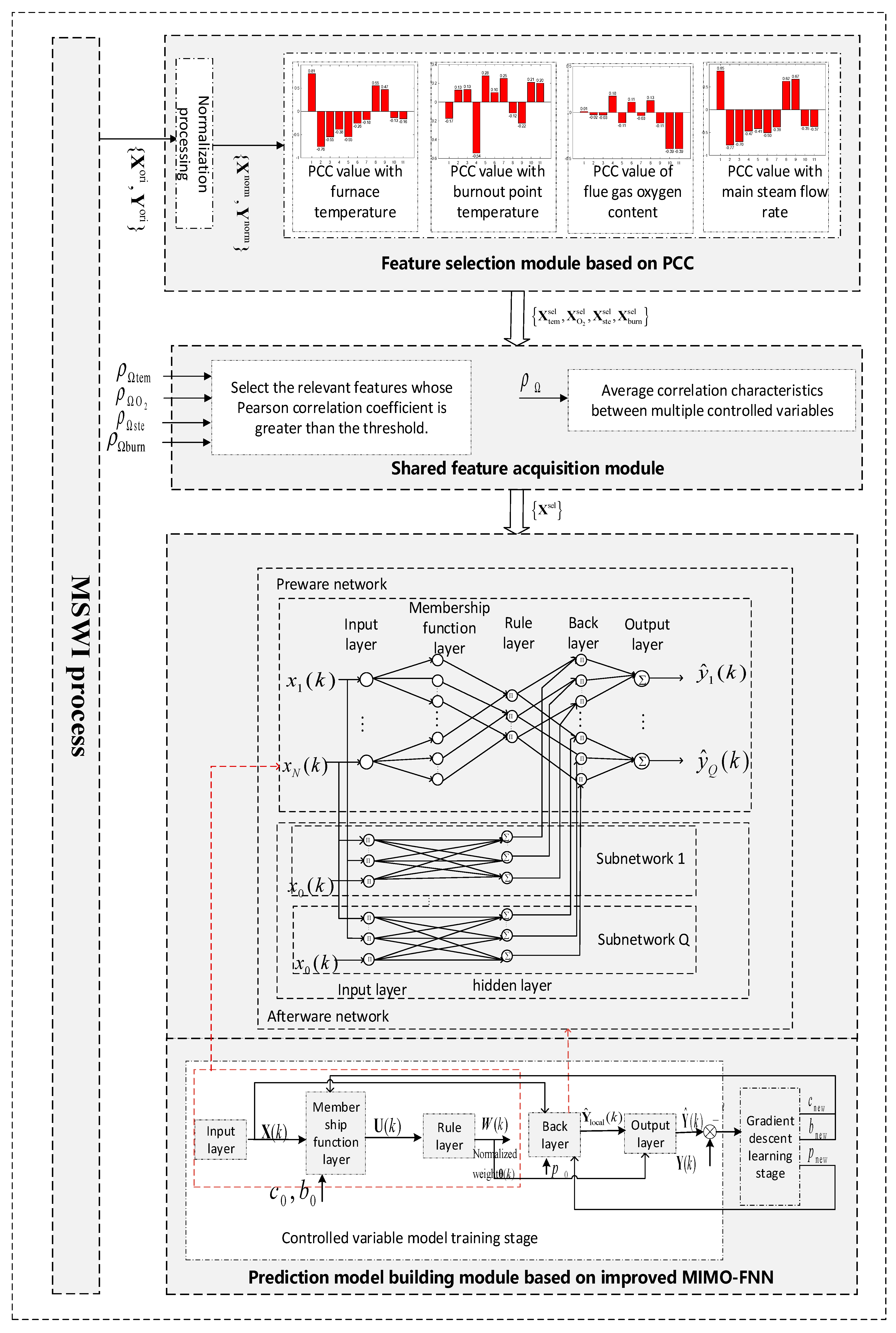
According to the technological characteristics of MSWI process, the MSWI multi-controlled variable prediction modeling strategy based on shared features and improved MIMO-FNN proposed in this article is shown in Figure 2.

Figure 2. Strategy diagram of the MSWI multi-controlled variable prediction modeling based on shared features and the improved MIMO-FNN modeling strategy.

In Figure 2, $\{X^{\mathrm{ori}},Y^{\mathrm{ori}}\}$ represents the original dataset; $\{X^{\mathrm{norm}},Y^{\mathrm{norm}}\}$ represents the normalized dataset; $\left\{X_{\mathrm{tem}}^{\mathrm{sel}},X_{{\mathrm{O}}_2}^{\mathrm{sel}},X_{\mathrm{ste}}^{\mathrm{sel}},X_{\mathrm{burn}}^{\mathrm{sel}}\right\}$ represents the dataset selected by PCC; ${\rho }_{\Omega },{\rho }_{\Omega \mathrm{tem}},{\rho }_{\Omega {\mathrm{O}}_2},{\rho }_{\Omega \mathrm{ste}}$ and ${\rho }_{\Omega \mathrm{burn}}$ represent the set PCC threshold; $\left\{X^{\mathrm{sel}}\right\}$ represents a dataset that has been redundantly merged; $X(k)$ represents input data entering an improved MIMO-FNN train module; The parameters $p_0,c_0$ and $b_0$ represent the initial setting; $U(k)$ represents the degree of membership calculated by the membership function layer; $W(k)$ represents the activation intensity calculated by the rule layer; $\theta (k)$ represents the weight after normalizing the activation intensity; ${\widehat{Y}}_{\mathrm{local}}(k)$ represents the local output of the improved MIMO-FNN training model; $\widehat{Y}(k)$ represents the predicted output of the improved MIMO-FNN training model; $Y(k)$ represents a true value; $p_{\mathrm{new}},c_{\mathrm{new}}$ and $b_{\mathrm{new}}$ represent the parameters updated by the gradient descent algorithm; $k$ represents the $k$-th sample.

The functions of each module in Figure 2 are as follows:

(1)

Feature selection module based on PCC. The original data $\{X^{\mathrm{ori}},Y^{\mathrm{ori}}\}$ are normalized to obtain $\{X^{\mathrm{norm}},Y^{\mathrm{norm}}\}$. T, the Pearson correlation coefficient between manipulated variables and each controlled variable (i.e., furnace temperature, flue gas oxygen content, main steam flow rate, and burnout point temperature), is calculated, and the output variable is recorded as $\left\{X_{\mathrm{tem}}^{\mathrm{sel}},X_{{\mathrm{O}}_2}^{\mathrm{sel}},X_{\mathrm{ste}}^{\mathrm{sel}},X_{\mathrm{burn}}^{\mathrm{sel}}\right\}$.

(2)

Shared feature acquisition module. Based on the different PCC thresholds set by each controlled variable and the average correlation between multiple controlled targets, the feature vectors $\{X^{\mathrm{norm}},Y^{\mathrm{norm}}\}$ are eliminated and merged, and recorded as $X^{\mathrm{sel}}$.

(3)

Prediction model building module based on improved MIMO-FNN. Taking the input variables $X(k)$ as the training module of the improved MIMO-FNN, the parameters are updated through the five-layer network structure and gradient descent method, and finally the model calculation output is recorded as $\widehat{Y}(k)$.

2.2.1. Data Preprocessing

Normalization Method

To eliminate dimensional differences between features and improve model convergence speed, this study employs min–max normalization to linearly transform the original data, mapping each feature value to the [0, 1] interval.

Normalization Formula:

$$x_i^{\mathrm{norm}} (k)={\displaystyle \frac{x_i (k)-\min (x_i ) }{\max (x_i )-\min (x_i)}}$$

(1)

Parameter Description: $x_i(k)$. The $k$-th original sample value of the $i$-th feature, where, $i=1,2,\dots 11;k=1,2,\dots K$; $\min (x_i)$: the minimum value of the $i$-th feature in the training set; $\max (x_i)$: the maximum value of the $i$-th feature in the training set; $x_i^{\mathrm{norm}} (k)$: the normalized feature value (within [0, 1] interval)

According to the above normalization formula, we can obtain that the normalized empty set is defined as:

$$D^{\mathrm{norm}}={\{x^{\mathrm{norm}}(k),y^{\mathrm{norm}}(k)\}}_{k=1}^K$$

(2)

where:

$$x^{\mathrm{norm}}(k)={[x_i^{\mathrm{norm}}(k)]}_{i=1}^I=[x_1^{\mathrm{norm}}(k),\cdots ,[x_I^{\mathrm{norm}}(k)]]$$

(3)

is the $k$-th sample vector of $x^{\mathrm{norm}}$, $k$ indicating the number of samples, $I=11$;

$$y^{\mathrm{norm}}(k)={[y_q^{\mathrm{norm}}(k)]}_{q=1}^Q={[y_1^{\mathrm{norm}}(k),\cdots ,y_Q^{\mathrm{norm}}(k)]}^T$$

(4)

is the $k$-th sample vector of $y^{\mathrm{norm}}$, $Q=4$.

Inverse Normalization Method

To restore model predictions to the original data scale for interpretation and practical application, inverse normalization is performed using the extreme value parameters saved during the normalization phase.

Inverse Normalization Formula:

$$y_q(k)=y_q^{\mathrm{norm}}(k)\times [\max (y_q)-\min (y_q)]+\min (y_q)$$

(5)

Parameter Description:

$y_q(k)$: the model’s normalized prediction output.

$\max (y_q),\min (y_q)$: minimum and maximum values of the target variable in the training set (saved during normalization).

$y\left(k\right)$: final prediction value after inverse normalization (original scale).

2.2.2. Feature Selection Module Based on PCC

Facing the modeling requirements of MSWI process in developing countries such as China, this module firstly carries out feature reduction based on the original manipulated variables collected on-site and expert experience. By calculating PCC values between multiple manipulated variables and four controlled variables (flue gas oxygen content, furnace temperature, main steam flow rate, and burnout point), redundant and noisy features are eliminated. In this study, based on PCC, the Pearson correlation coefficient between each manipulated variable and the furnace temperature, flue gas oxygen content, main steam flow, and burnout point temperature is calculated.

The specific calculation process is as follows:

Calculate the PCC value of the $i$-th input and the $q$-th output according to the following formula:

$${\rho }_{iq}={\displaystyle \frac{K{\displaystyle \sum _{k=1}^K(x_i^{\mathrm{norm}}(k)-{\overline{x}}_i^{\mathrm{norm}}(k))(y_q^{\mathrm{norm}}(k)-{\overline{y}}_q^{\mathrm{norm}}(k))}}{\sqrt{K{\displaystyle \sum _{k=1}^K{(x_i^{\mathrm{norm}}(k)-{\overline{x}}_i^{\mathrm{norm}}(k))}^2}}\sqrt{K{\displaystyle \sum _{k=1}^K{(y_q^{\mathrm{norm}}(k)-{\overline{y}}_q^{\mathrm{norm}}(k))}^2}}}}$$

(6)

where $x_i^{\mathrm{norm}}(k)$ is the $k$-th sample vector of the $i$-th input; $y_q^{\mathrm{norm}}(k)$ is the $i$-th sample vector of the $q$-th output; and ${\rho }_{iq}$ is the PCC values of the i-th input and the $q$-th output.

2.2.3. Shared Feature Acquisition Module

In the context of multi-variable control optimization, to achieve efficient and robust feature extraction, this study manually selected the manipulated variables with significant influence from the process variables for the four key output variables: furnace temperature, flue gas oxygen content, main steam flow rate, and burnout point. During the screening process, both the average correlation with multiple controlled variables and the highest correlation with a single target are considered. The following steps outline the specific operations as follows.

Firstly, based on PCC, the threshold value related to the controlled variable is recorded as follows:

$${\rho }_{\Omega q }=[{\rho }_{\Omega },{\rho }_{\Omega \mathrm{tem}},{\rho }_{\Omega {\mathrm{O}}_2},{\rho }_{\Omega \mathrm{ste}},{\rho }_{\Omega \mathrm{burn}}]$$

(7)

where ${\rho }_{\Omega }$ is the set average maximum PCC value; ${\rho }_{\Omega \mathrm{tem}}$ is the set furnace temperature PCC value; ${\rho }_{\Omega {\mathrm{O}}_2}$ is the set PCC value of flue gas oxygen content; ${\rho }_{\Omega \mathrm{ste}}$ is the set PCC value of main steam flow; and ${\rho }_{\Omega \mathrm{ste}}$ is the set burning point temperature PCC value.

The features highly related to the controlled variables are screened out by the following decision rules:

$${\xi }_{\Omega }=\left\{\begin{array}{l}1, if {\rho }_{iq}\ge {\rho }_{\Omega q }\\ 0, if {\rho }_{iq}<{\rho }_{\Omega q }\end{array}\right.$$

(8)

where ${\xi }_{\Omega }=1$ indicates that the feature is selected. Through this rule, the furnace temperature, flue gas oxygen content, main steam flow rate, and burnout point temperature are operated, and the sub-features significantly related to the controlled variables are screened out and combined to form a preliminary process feature set.

Based on the different settings ${\rho }_{\Omega q }$ of each controlled variable and the average correlation between multiple controlled targets, $I^{\prime }$ feature vectors are obtained $X^{\mathrm{norm}}={\left\{x^{\mathrm{norm}}(k)\right\}}_{k-1}^K\in {ℝ}^{K\times I}$, and the dataset after feature reduction is as follows:

$$\left\{X_{\mathrm{tem}}^{\mathrm{sel}},X_{{\mathrm{o}}_2}^{\mathrm{sel}},X_{\mathrm{ste}}^{\mathrm{sel}},X_{\mathrm{burn}}^{\mathrm{sel}}\right\}=f_{\mathrm{PCC}}\left(X^{\mathrm{norm}}\right)$$

(9)

where $\left\{X_{\mathrm{tem}}^{\mathrm{sel}},X_{{\mathrm{o}}_2}^{\mathrm{sel}},X_{\mathrm{ste}}^{\mathrm{sel}},X_{\mathrm{burn}}^{\mathrm{sel}}\right\}$ is the shared feature dataset after feature selection based on PCC, with the total number of features as $I^{\prime }$, the existence of $I^{\prime }\le I$ is recorded as:

$$X_{\mathrm{norm}}^{\mathrm{sel}}={\left\{x_{\mathrm{norm}}^{\mathrm{sel}}(k)\right\}}_{k=1}^K\in {ℝ}^{K\times I^{\prime }}$$

(10)

where:

$$\left\{X_{\mathrm{norm}}^{\mathrm{sel}}(k)\right\}=\left\{X_{\mathrm{tem}}^{\mathrm{sel}}(k),X_{{\mathrm{o}}_2}^{\mathrm{sel}}(k),X_{\mathrm{ste}}^{\mathrm{sel}}(k),X_{\mathrm{burn}}^{\mathrm{sel}}(k)\right\}$$

(11)

where $f_{\mathrm{PCC}}\left(\cdot \right)$ represents the function selected by PCC.

2.2.4. Prediction Model Building Module Based on Improved MIMO-FNN

The fuzzy neural network [38] based on Takagi–Sugeno (TS) is adopted, and its structure usually includes antecedent network and posterior network.

Antecedent Network

The antecedent network is responsible for the fuzzification of input data and the calculation of rule activation intensity. The process is detailed as follows.

(1)

Input layer:

The function is to receive input data and send it to subsequent layers. The input vector of the k-th sample is recorded as:

$$X(k)={[x_1(k),\cdots ,x_2(k),\cdots ,x_{I^{\prime }}(k)]}^T\in {ℝ}^{I^{\prime }\times 1}$$

(12)

(2)

Membership function layer:

The function is to transform the accurate input into a fuzzy set through Gaussian membership function and to realize the fuzzy division of feature space. The membership matrix with $X(k)$ as and output as is recorded as:

$$U(k)\in {ℝ}^{I^{\prime }\times M}$$

(13)

The membership value of the i-th input corresponding to the j-th rule is calculated as follows:

$$u_{ij}(k)=\exp (-\min ({\displaystyle \frac{{(x_i(k)-c_{ij}(k))}^2}{\max (b_{ij}(k),0.1)}} ,100))+ϵ$$

(14)

where $c_{ij}(k)$ is the center of the membership function of the $i$-th input corresponding to the $j$-th rule; $b_{ij}(k)$ is the width of the membership function of the $i$-th input corresponding to the $j$-th rule; $\max (b_{ij}(k),0.1)$ and $\min (\cdots ,100)$ is a numerical stability technique to prevent exponential explosion caused by too small denominator or underflow caused by too large exponent; and $ϵ={10}^{-20}$ is to ensure that the membership degree is never zero and avoid mistakes in subsequent division calculation.

(3)

Rule layer:

The function is to use fuzzy multiplication operator as fuzzy logic rules and calculate the activation intensity of each fuzzy rule. The intensity vector with $U(k)$ as and output as activation is recorded as:

$$W(k)={[w_1(k),w_2(k),\cdots ,w_M(k)]}^T\in {ℝ}^{M\times 1}$$

(15)

The activation intensity under the $j$-th rule is calculated as follows:

$$w_j(k)=\max ({\displaystyle \prod _{i=1}^N{u}_{ij}}(k) ,ϵ)$$

(16)

where $\max (\cdots ,ϵ)$ is also a measure to ensure the numerical stability, ensuring $w_j>0$.

The output weight of normalized deblurring $W(k)$ is recorded as:

$$\theta (k)={[{\theta }_1(k),{\theta }_2(k),\cdots ,{\theta }_M(k)]}^T\in {ℝ}^{M\times 1}$$

(17)

The activation weight under the $j$-th rule is calculated as:

$${\theta }_j(k)=w_j(k)/\max ({\displaystyle \prod _{j=1}^M{w}_j}(k) ,ϵ)$$

(18)

where $ϵ={10}^{-20}$ is a minimal positive number to prevent the weight from being zero.

The output of this part is the activation intensity of each rule, which is used as the weight of the posterior network.

Posterior Network

The latter network is responsible for local linear modeling and global output synthesis according to the regular activation intensity of the former network output, and its process is as follows.

(1)

Rear piece layer:

The function is to calculate the parameters of the output corresponding to each rule. The input is as follows:

$$X(k)\in {ℝ}^{(I^{\prime }+1)\times 1}$$

(19)

where:

$$X(k)={[1,x_1(k),x_2(k),\cdots ,x_{I^{\prime }}(k)]}^T$$

(20)

and the output is a local output, which is recorded as follows:

$${\widehat{Y}}_{\mathrm{local}}(k)\in {ℝ}^{M\times Q}$$

(21)

The $j$-th fuzzy rule corresponds to the local prediction of the $q$-th output is calculated as follows:

$${\widehat{y}}_{j,\mathrm{local}}^q(k)={\displaystyle \sum _{i=0}^N{p}_{ij}^q}•x_i(k)=p_{0j}^q\left(k\right)x_0\left(k\right)+p_{1j}^q(k)x_1\left(k\right)+\dots +p_{Nj}^q\left(k\right)x_{I^{\prime }}\left(k\right)$$

(22)

where:

$$p_{ij}^q\in {ℝ}^{(I^{\prime }+1)\times M}$$

(23)

is the posterior parameter matrix of the system,

(2)

Output layer

The function is the final output of weighted average of local output. Its input is activation intensity $W(k)$. The local output and the output of ${\widehat{Y}}_{\mathrm{local}}(k)$ and the output as the final vector are recorded as:

$$\widehat{Y}(k)={[{\widehat{y}}_1(k),{\widehat{y}}_2(k),\cdots ,{\widehat{y}}_Q(k)]}^T$$

(24)

The predicted value of the q-th output variable is calculated as follows:

$${\widehat{y}}_q(k)={\displaystyle \sum _{j=1}^M{\theta }_j(k)}{\widehat{y}}_{j,\mathrm{local}}^q(k)$$

(25)

This part combines the antecedent and afterpart of fuzzy rules to complete the mapping from input to output.

Model Parameter Learning

The model uses gradient descent method [39] to update the parameters, and the related algorithms are defined as follows.

The Huber loss function [40] is defined as follows:

$$L_{\delta }\left(r_q\right)=\left\{\begin{array}{l}{\displaystyle \frac{1}{2}}{r}_q^2, \mathrm{if}\left|r_q\right|\le \delta \\ \delta \left|r_q\right|-{\displaystyle \frac{1}{2}}{\delta }^2, \mathrm{otherwise}\end{array}\right.$$

(26)

The Huber loss derivative function is as follows:

$${\displaystyle \frac{\partial L_{\delta }\left(r_q\right)}{\partial r_q}}=\left\{\begin{array}{l}{r}_q, \mathrm{if}\left|r_q\right|\le \delta \\ \delta sign\left(r_q\right), \mathrm{otherwise}\end{array}\right.$$

(27)

$$r_q\left(k\right)={\displaystyle \frac{y_q\left(k\right)-{\widehat{y}}_q\left(k\right)}{\max \left(\left|y_q\left(k\right)\right|,\epsilon \right)}}$$

(28)

where $r_q\left(k\right)$ is the relative error, $\delta$ is the Huber loss threshold parameter, $y_q\left(k\right)$ is the true value of the $q$-th output of the $k$-th sample, and ${\widehat{y}}_q(k)$ is based on the predicted value of the $q$-th output of the $k$-th sample based on the improved MIMO-FNN model.

The total loss function is defined as follows:

$$L_{\mathrm{total}}={\displaystyle \sum _{q=1}^Q{L}_{\delta }\left(r_q\right)}$$

(29)

Further, the post-processing parameters are updates as follows:

$$p_{ij}\left(k+1\right)=p_{ij}\left(k\right)+{\eta }_3{\displaystyle \frac{\partial L_{\mathrm{total}}}{\partial p_{ij}\left(k\right)}}+\alpha \left(p_{ij}\left(k\right)-p_{ij}\left(k-1\right)\right)$$

(30)

The width parameter is updated as:

$$b_{ij}\left(k+1\right)=b_{ij}\left(k\right)+{\eta }_1{\displaystyle \frac{\partial L_{\mathrm{total}}}{\partial b_{ij}\left(k\right)}}+\alpha \left(b_{ij}\left(k\right)-b_{ij}\left(k-1\right)\right)$$

(31)

The central parameter is updated as:

$$c_{ij}\left(k+1\right)=c_{ij}\left(k\right)+{\eta }_2{\displaystyle \frac{\partial L_{\mathrm{total}}}{\partial c_{ij}\left(k\right)}}+\alpha \left(c_{ij}\left(k\right)-c_{ij}\left(k-1\right)\right)$$

(32)

This module ensures that the model can improve the prediction accuracy and generalization ability through continuous learning and optimization parameters.

2.3. Pseudocode and Flow Chart of the Algorithm Pseudocode

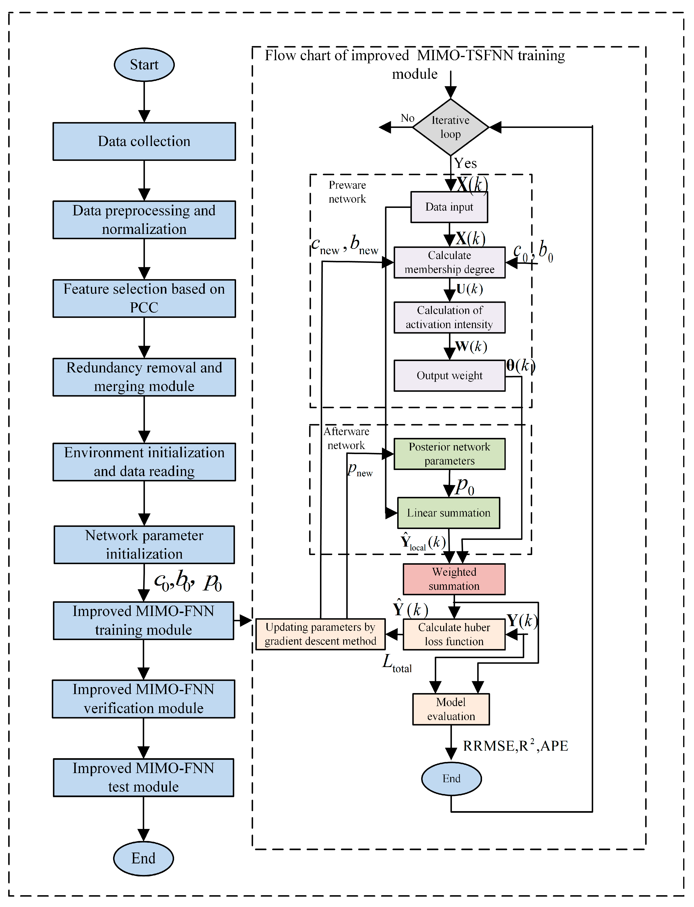
The pseudocode of the Algorithm 1 used in this article is as follows (Figure 3).

Algorithm 1 Improved MIMO-FNN
Step 1:	Input. training dataset $\left\{X,Y\right\}$, number of input nodes $I^{\prime }$, number of output nodes $Q$, number of hidden nodes $M$, maximum number of iterations $\max gen$, and learning rate $\eta$;
Step 2:	Initialization. randomly initialize the fuzzy posterior parameters $p_0$; randomly initialize the center $c_0$ and width of membership $b_0(b_0\ge 0.1)$; record the historical array of each parameter;
Step 3:	For iteration = 1 to max_iterations do, outer cyclic iterative algebra;
Step 4:	For k = 1 to SamNum do, inner loop over training samples
Step 5:	Read the k-th sample;
Step 6:	Calculate Gaussian membership degree $u_{ij}(k)$ and activation intensity $w_j(k)$ based on Equations (13) and (14);
Step 7:	Calculate that local conclusion of each output ${\widehat{y}}_{q,\mathrm{local}}(k)$ and the network output ${\widehat{y}}_q(k)$ based on Equations (21)–(24);
Step 8:	Calculate the relative error $r_q\left(k\right)$ and total error $L_{\mathrm{total}}$ of each output based on Equations (25)–(27);
Step 9:	Update membership parameters $b_{\mathrm{new}}$ and $c_{\mathrm{new}}$, based on Equations (30) and (31);
Step 10:	Update the post-processing parameters, based on Equation (29);
Step 11:	End;
Step 12:	Calculate and record the RRMSE and R2 indicators of this iteration based on Equations (32) and (33);
Step 13:	End;
Step 14:	Verification. Repeat steps 5–7 to forward calculate the verification set; Calculate and visualize the verification sets RRMSE, APE and R2 according to Equations (32) and (33);
Step 15:	Test. Repeat steps 5–7 for forward calculation of the test set; Calculate the test set RRMSE, APE, R2 according to Formulas (32)–(34) and visualize it;
Step 16:	Output;

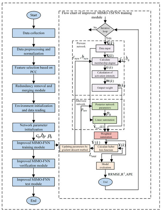
Figure 3. Flow chart of improved MIMO-FNN model.

3. Results

3.1. Performance Metrics

This study selected the relative root mean square error (RRMSE), average percentage error (APE), and determining coefficient (R-squared, R²) to evaluate the modeling effect, and the relevant definitions are as follows.

$${\mathrm{RRMSE}}_q=\sqrt{{\displaystyle \frac{1}{K}}{\displaystyle \sum _{k=1}^K\left(\frac{{\left(y_q(k)-{\widehat{y}}_q(k)\right)}^2}{y_q(k)}\right)}}$$

(33)

$${\mathrm{APE}}_q={\displaystyle \frac{1}{K}}{\displaystyle \sum _{k=1}^K\left|\frac{{\left(y_q(k)-{\widehat{y}}_q(k)\right)}^2}{y_q(k)}\right|}\times 100\%$$

(34)

$${\mathrm{R}}_q^2=1-{\displaystyle \frac{{\displaystyle \sum _{k=1}^K{\left(y_q\left(k\right)-{\widehat{y}}_q\left(k\right)\right)}^2}}{{\displaystyle \sum _{k=1}^K{(y_q\left(k\right)-{\overline{y}}_q)}^2}}}$$

(35)

where $y$ is the actual value, $\widehat{y}$ is the predicted value, and $\widehat{y}$ is the average of the actual values.

3.2. Experimental Results

In this study, the sampling frequency of a MSWI power plant in Beijing is 1 s/time, and 3000 groups of data on one day of March 2021 are selected, of which 60% are the training set, 20% are the validation set, and 20% are the test set. In this section, the corresponding experiments are carried out for feature reduction, model training, verification and testing of the controlled object, and the results are as follows.

3.2.1. Feature Selection Results

Correlation Between Manipulated Variables and Furnace Temperature

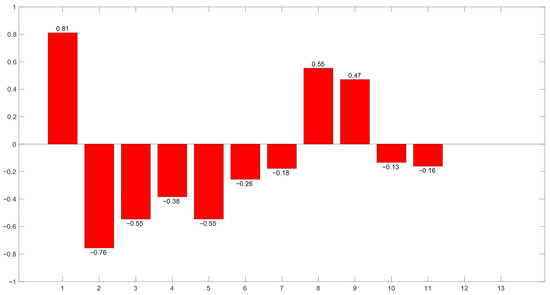
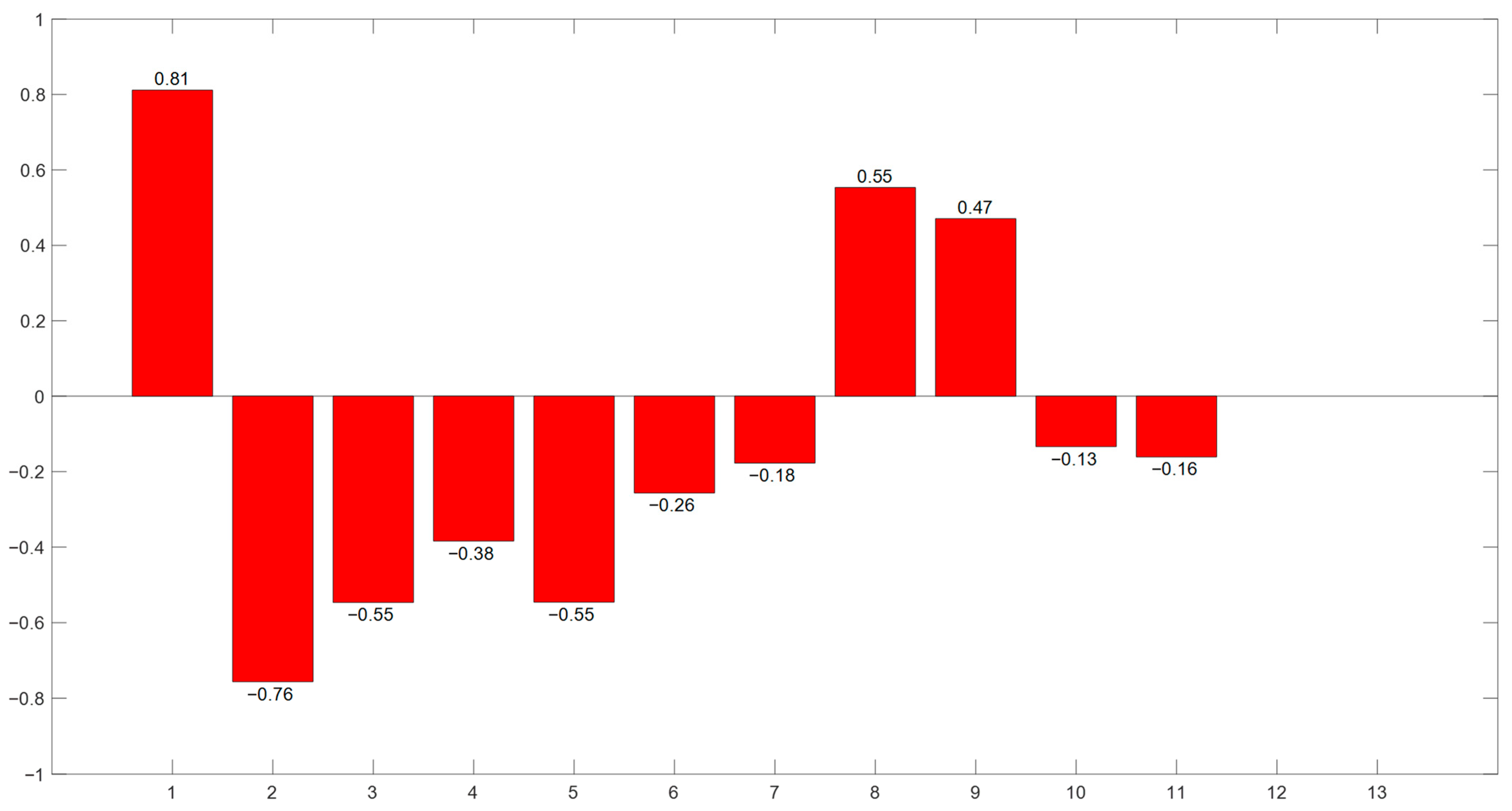
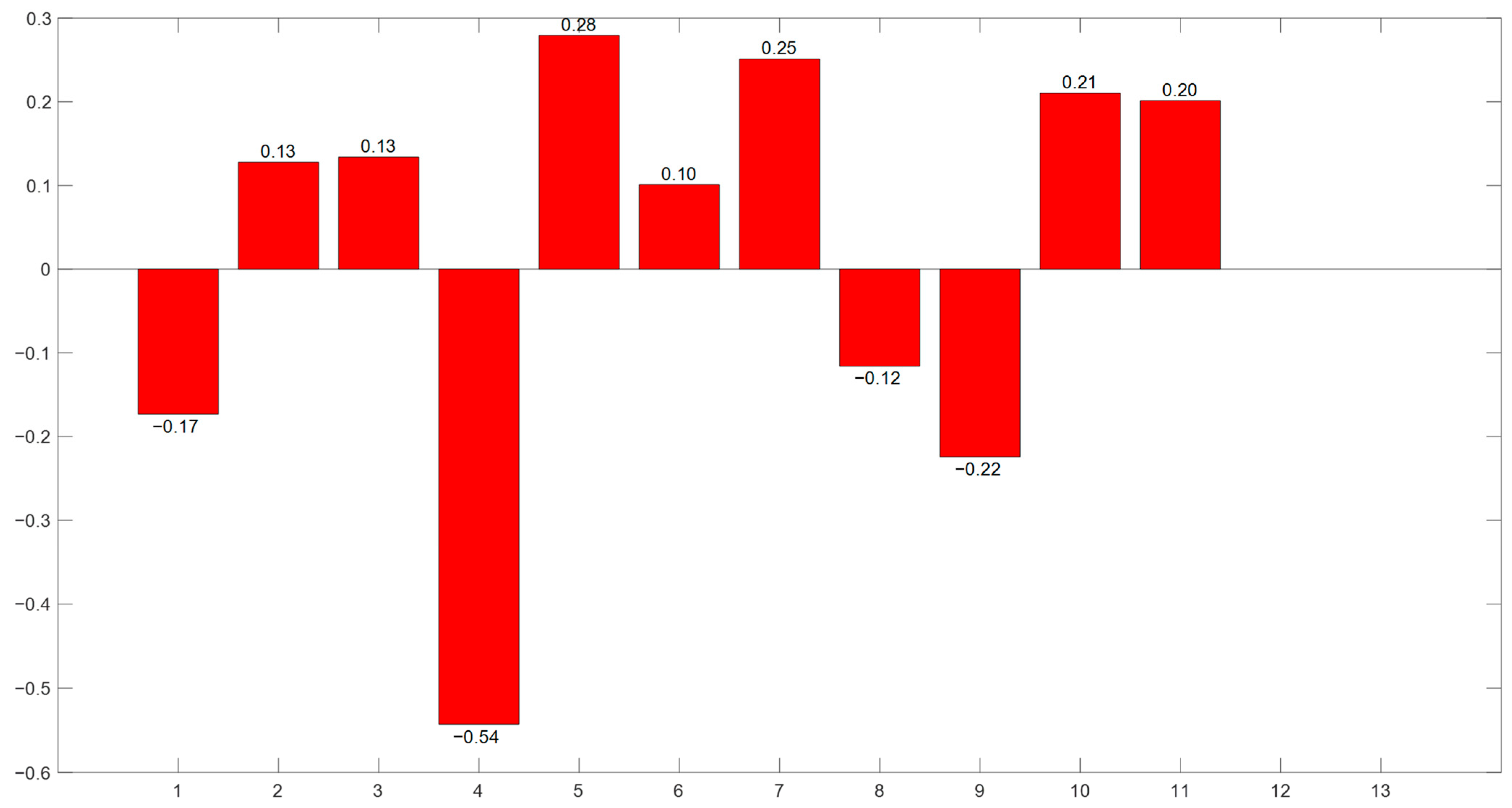
The Pearson correlation coefficients between the manipulated variables and the furnace temperature is shown in Figure 4.

Figure 4. The Pearson correlation coefficients between the manipulated variables and the furnace temperature.

According to Figure 4, the results of the Pearson correlation coefficient analysis indicate that most manipulated variables are positively correlated with furnace temperature, while a few exhibit a negative correlation. By examining the absolute values, it can be determined that the manipulated variables highly correlated with furnace temperature include: primary air temperature, primary air volume, primary air pressure, secondary air temperature, secondary air volume, air volume in the drying section, air volume in combustion Section 1, air volume in combustion Section 2, feeding speed, and grate speed in the drying section, with corresponding PCC values of 0.8117, 0.7564, 0.5468, and 0, respectively. Among these variables, primary air temperature and total primary air volume are identified as having the most significant influence on furnace temperature.

Correlation Between Manipulated Variables and Flue Gas Oxygen Content

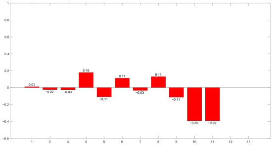
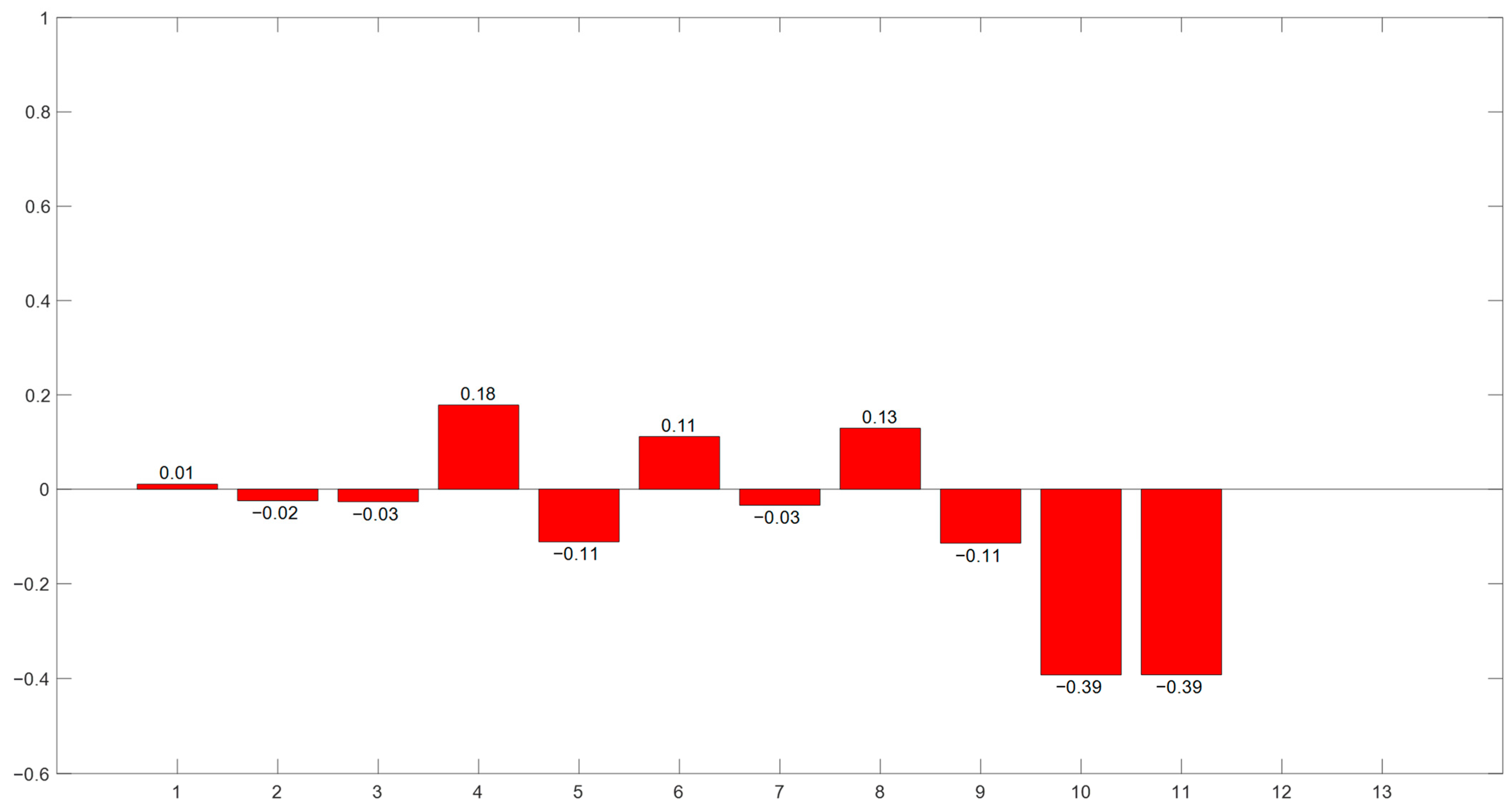
The Pearson correlation coefficients between the manipulated variables and flue gas oxygen content is shown in Figure 5.

Figure 5. The Pearson correlation coefficients between the manipulated variables and the flue gas oxygen content.

According to Figure 5, the results of the Pearson correlation coefficient analysis for the manipulated variables and flue gas oxygen concentration indicate that the correlation between the manipulated variables and oxygen content is generally weak, with most variables exhibiting a positive correlation. An analysis of the absolute PCC values reveals that feeding speed and grate speed in the drying section have the most significant influence on flue gas oxygen content, with corresponding PCC values of 0.3924 and 0.3921, respectively. The air flow rate in the drying section also exerts some influence, with a PCC value of 0.1785. Other variables, including secondary air temperature, secondary air volume, and air flow rates in the first and second stages of combustion, are positively correlated; however, the correlations are weak, with all PCC values falling below 0.13. The influence of primary air temperature, primary air volume, primary air pressure, and air flow rate in the combustion sections on flue gas oxygen concentration is minimal, as indicated by PCC values that remain below 0.04.

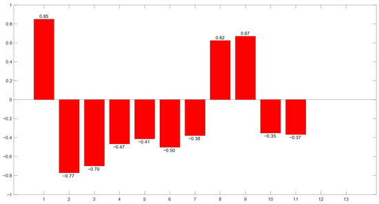
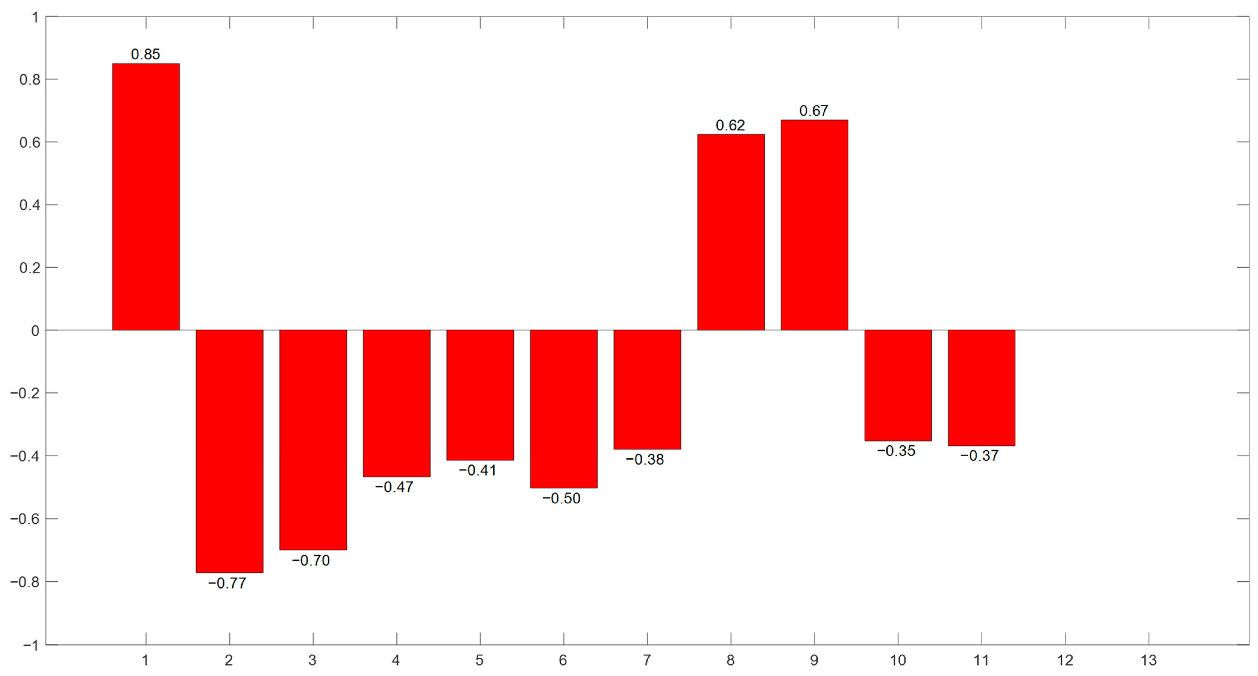
Correlation Between Manipulated Variables and Main Steam Flow

The Pearson correlation coefficients between the manipulated variables and main steam flow are shown in Figure 6.

Figure 6. The Pearson correlation coefficients between the manipulated variables and main steam flow.

According to Figure 6, the results of the Pearson correlation coefficient analysis for the manipulated variables and main steam flow indicate a significant positive correlation between each of the manipulated variables and main steam flow. An analysis of the absolute PCC values reveals that primary air temperature has the most substantial influence on steam flow, with a PCC value of 0.8498. The total primary air flow rate and primary air pressure also exert a strong influence, with PCC values of 0.7717 and 0.6998, respectively. The influence of secondary air volume and secondary air temperature is the next most significant, with PCC values of 0.6697 and 0.6243, respectively. Additionally, the air flow rates in the second stage of combustion, drying stage, and first stage of combustion exhibit a moderate correlation with steam flow, with PCC values of 0.5031, 0.4675, and 0.4147, respectively. The effects of feed rate, grate speed in the drying section, and air flow rate in the combustion section are relatively weak, as indicated by PCC values that remain below 0.38.

Correlation Between Manipulated Variables and Burnout Point Temperature

The Pearson correlation coefficients between the manipulated variables and burnout point temperature are shown in Figure 7.

Figure 7. The Pearson correlation coefficients between the manipulated variables and burnout point temperatures.

According to Figure 7, the results of the Pearson correlation coefficient analysis for the manipulated variables and burnout temperature indicate that the correlation between each variable and the burnout point temperature, with the overall correlation strength being weaker compared to its influence on steam flow. An analysis of the absolute PCC values reveals that the correlation between the air flow rate in the drying section and the burnout point is the highest, with a PCC value of 0.5429. The secondary air volume, air flow rate in the first stage of combustion, and air flow rate in the combustion stage also demonstrate some influence, with PCC values of 0.2243, 0.2793, and 0.2509, respectively. Additionally, the primary air temperature, total primary air flow rate, primary air pressure, secondary air temperature, air flow rate in the second stage of combustion, feed rate, and grate speed in the drying stage all exhibit weak correlations with the burnout point temperature, with PCC values remaining below 0.23.

3.2.2. Shared Feature Acquisition Results

The absolute Pearson correlation coefficient values were calculated between the manipulated variables of the model and the controlled variables, as shown in Table 2.

Table 2. Statistical table of absolute values of PCC between manipulated variables and controlled variables.

No.	Variable Name	Furnace Temperature	Flue Gas Oxygen Content	Main Steam Flow	Burnout Point	Average PCC
1	Primary air temperature	0.8117	0.0109	0.8498	0.1733	0.4614
2	Total amount of primary air	0.7564	0.0242	0.7717	0.1278	0.4200
3	Primary wind pressure	0.5468	0.0264	0.6998	0.1339	0.3517
4	Secondary air temperature	0.5532	0.1293	0.6243	0.1159	0.3557
5	Secondary air volume	0.4708	0.1143	0.6697	0.2243	0.3698
6	Air volume in drying section	0.3841	0.1785	0.4675	0.5429	0.3933
7	Combustion 1st stage air volume	0.5457	0.1113	0.4147	0.2793	0.3378
8	Combustion second stage air volume	0.2566	0.1118	0.5031	0.1009	0.2431
9	Air volume in combustion section	0.1773	0.0338	0.3797	0.2509	0.2104
10	Feeding speed	0.1337	0.3924	0.3685	0.2101	0.2762
11	Grate speed in drying section	0.1610	0.3921	0.3531	0.2013	0.2769

Based on the principles of maximizing the average Pearson correlation coefficient value, maximizing the PCC value, and encompassing various process stages, the following manipulated variables were selected. The primary air temperature was found to significantly influence steam flow and furnace temperature, yielding a maximum PCC value of 0.8498. The PCC value for primary air was calculated to be 0.7717, which directly affects combustion intensity and oxygen content in the furnace. The PCC value for the air flow in the drying section is determined to be 0.5429, demonstrating a pronounced effect on the burnout point and flue gas oxygen content. The maximum PCC value for secondary air volume is reported as 0.6697, which is utilized to regulate the oxygen content and steam production in the combustion zone. The PCC value for feed rate is measured at 0.3924, representing a key control parameter for fuel input and influencing flue gas oxygen content and the burnout point. The PCC value for grate speed in the drying section is noted to be 0.3921, which, in conjunction with the feed rate, determines the residence time of fuel in the furnace. In summary, the primary air temperature, primary air volume, air flow in the drying section, secondary air volume, feed rate, and drying furnace exhaust gas flow rate are identified as key manipulated variables, while furnace temperature, flue gas oxygen content, main steam flow rate, and burnout point are recognized as key controlled variables (Table 3).

Table 3. Manipulated variables feature combination result.

Category	Characteristic
Manipulated variable’s combination sign	Primary air temperature
	Total amount of primary air
	Air volume in drying section
	Secondary air volume
	Feeding speed
	Drying furnace discharge speed

3.2.3. Prediction Model Results

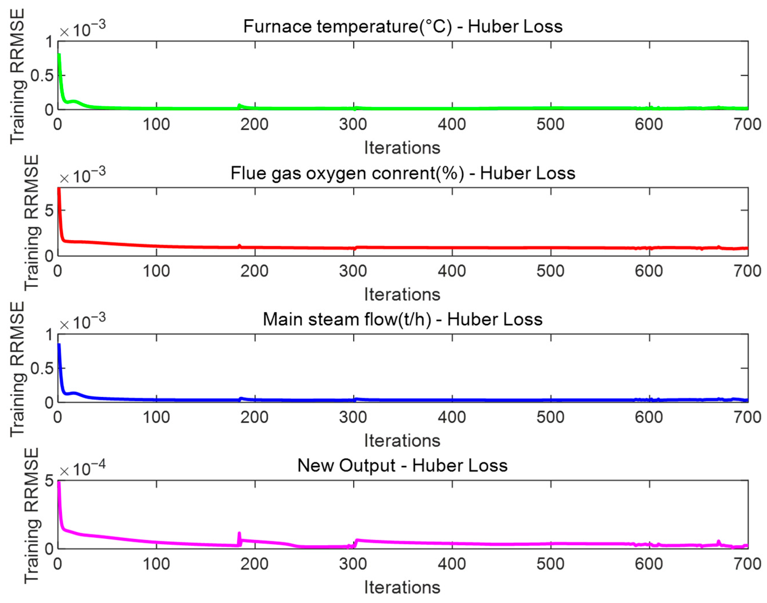
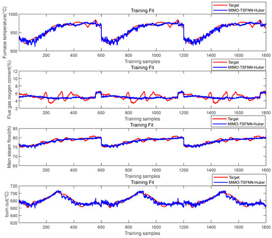
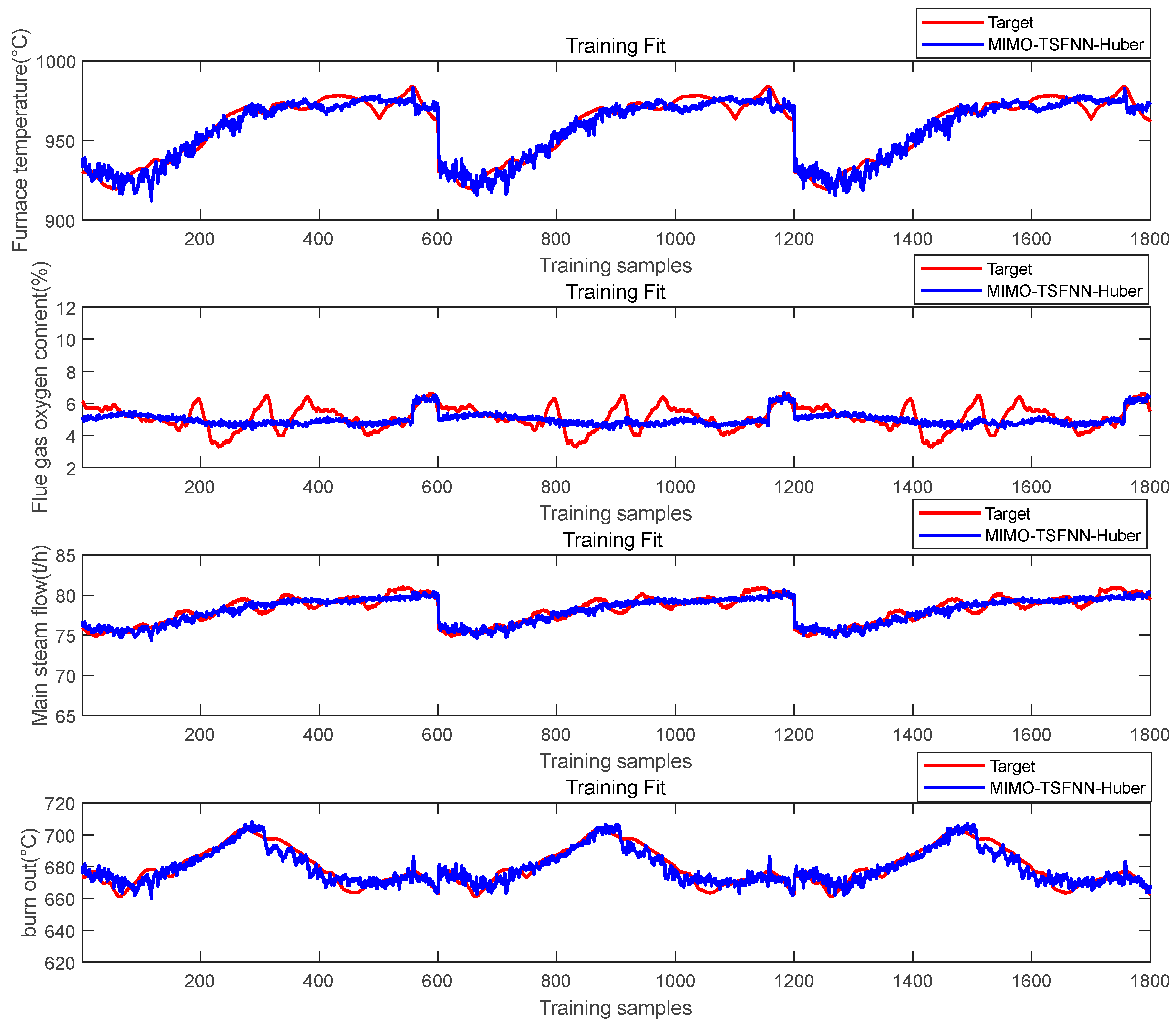
The improved MIMO-FNN model training module is based on feature reduction experiments and data processing. The parameters of the model are set as follows: 6 neurons in the input layer, 6 × 18 neurons in the membership function layer, 18 neurons in the regular layer, 18 × 4 neurons in the back layer, and 4 neurons in the output layer. The training iteration is deployed for 700 times. The RRMSE in the training process of the controlled object model is shown in Figure 8. The fitting effect of the training process of the model is shown in Figure 9.

Figure 8. Changes of RRMSE during model training.

Figure 9. Training sample fitting effect.

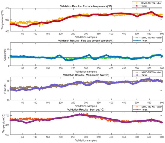
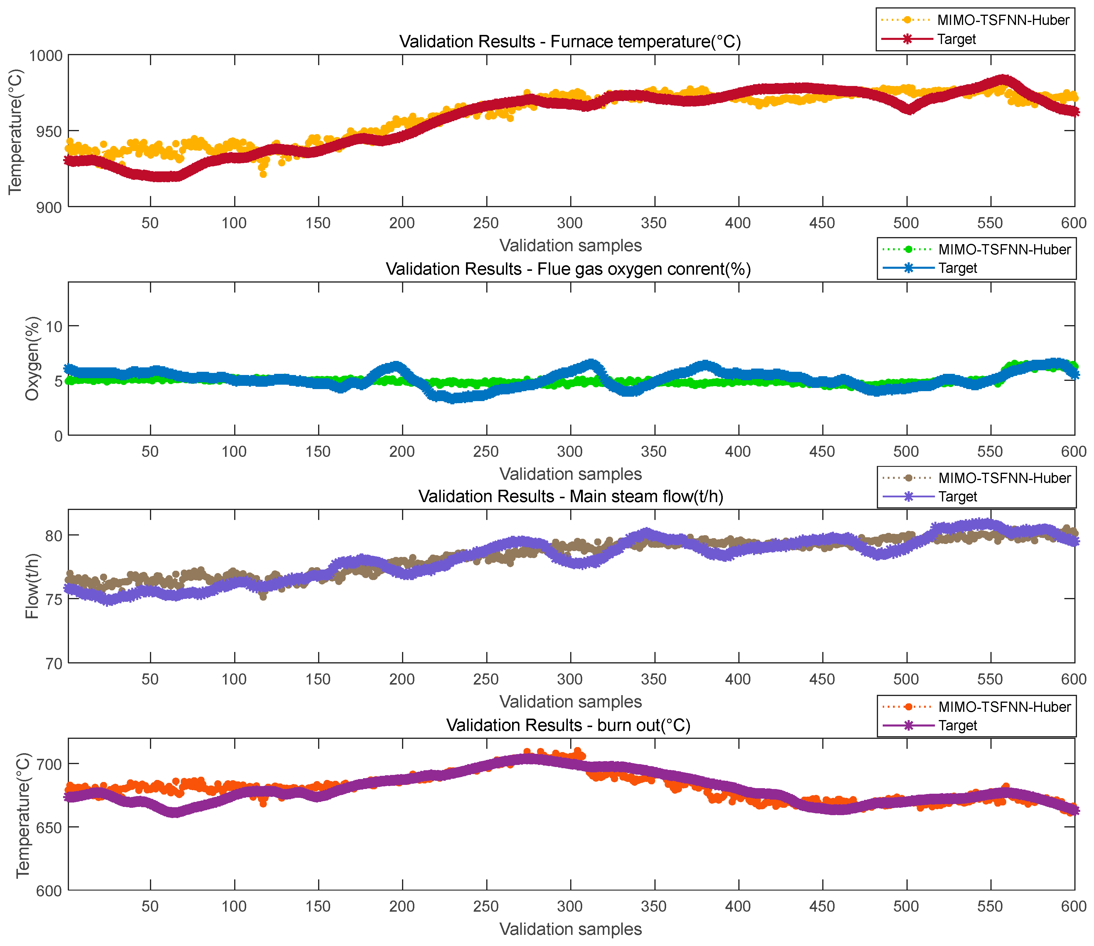
The validation and fitting effects of the model are shown in Figure 10.

Figure 10. Verify the sample fitting effect diagram.

Figure 10 shows that the model has good approximation ability in multi-output samples, takes into account the learning task of multi-sample output, and has good generalization ability.

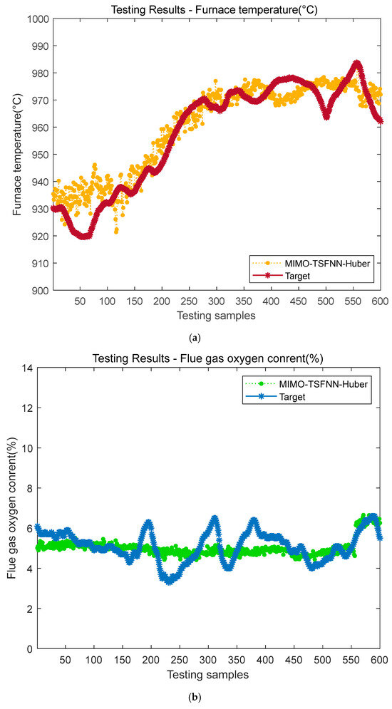
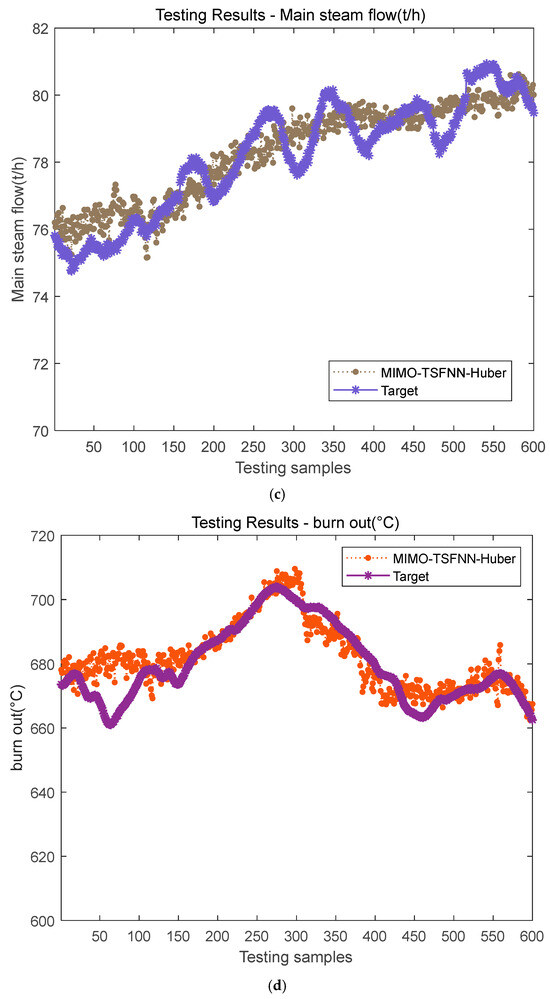
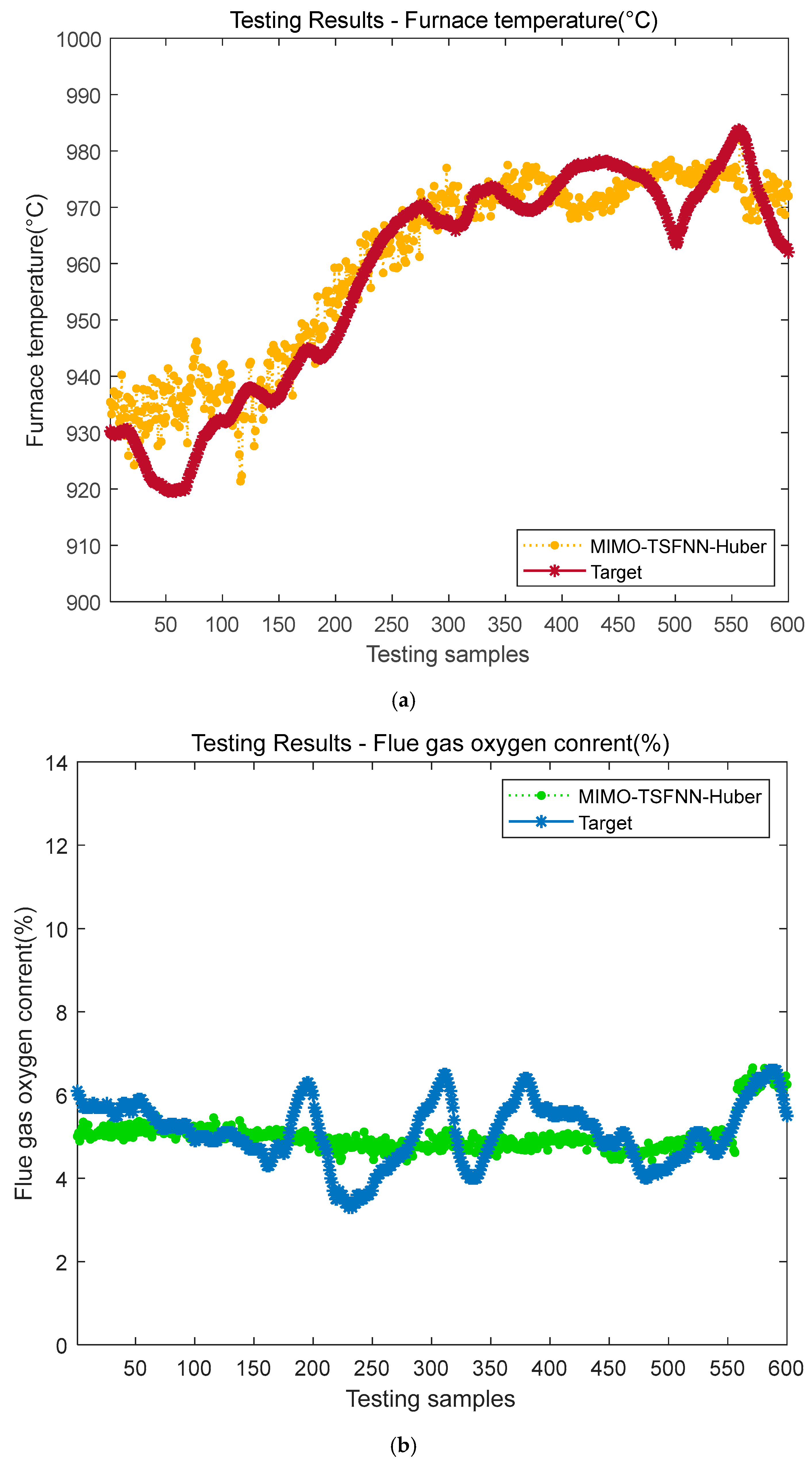
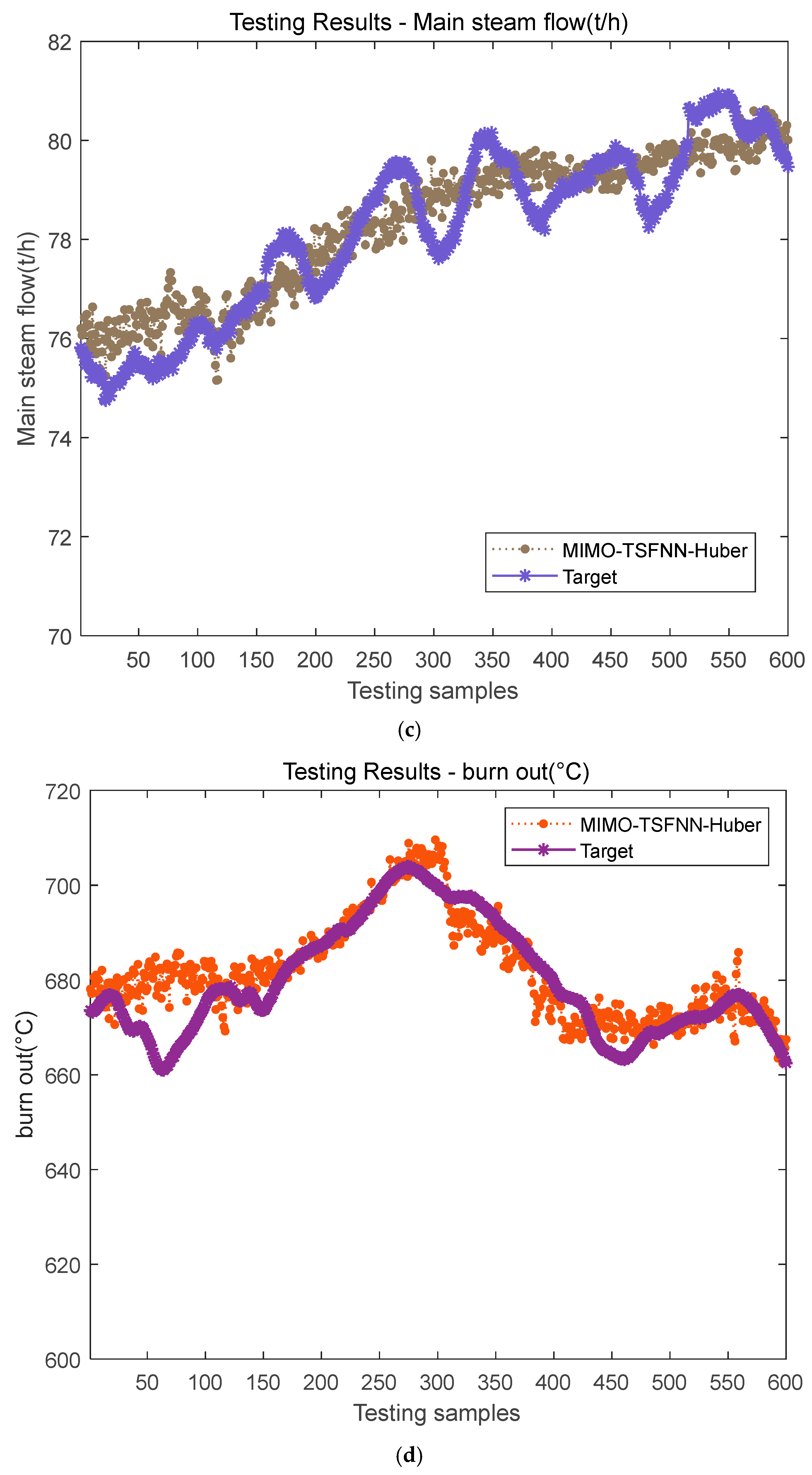
The test fitting effect of the model is shown in Figure 11.

Figure 11. (a) Furnace temperature test fitting effect diagram; (b) Flue gas oxygen content test fitting effect diagram; (c) Main steam flow test fitting effect diagram; (d) Burnout point temperature test fitting effect diagram.

Figure 11 shows that the model has good approximation ability in multi-output samples, takes into account the learning task of multi-sample output, and has good generalization ability.

3.3. Method Comparison

3.3.1. Modeling Methodology

The parameters of BPNN method are set as follows: the number of neurons in hidden layer is 12, the maximum convergence times is 500, the convergence error is 0.001, and the learning rate is 0.0001. The parameters of RBFNN method are set as follows: the number of neurons in hidden layer is 12, the maximum number of convergence is 500, and the learning rate is 0.002. The parameters of MIMO-TSFNN method are set as follows: the number of hidden layer neurons is 12, the maximum number of convergence is 500, the convergence error is 0.001, the learning rate of membership width is 0.001, and the membership center and posterior parameters are 0.002.

Compare the experimental results of BPNN, RBFNN, MIMO-TSFNN, and improved TSFNN with RRMSE and R² evaluation indexes, are shown in Table 4.

Table 4. Comparison of experimental results.

		BPNN		RBFNN		MIMO-TSFNN		Improved FNN
CV	DataSet	R2	RRMSE	R2	RRMSE	R2	RRMSE	R2	RRMSE
FT	Training set	0.8844 ± 0.0002	0.0069 ± 0.0000	0.8511 ± 0.0001	0.0078 ± 0.0000	0.9238 ± 0.0003	0.0056 ± 0.0000	0.9355 ± 0.0003	0.0000 ± 0.0000
	Verification set	0.8839 ± 0.0002	0.0069 ± 0.0000	0.7714 ± 0.0000	0.0082 ± 0.0000	0.9194 ± 0.0004	0.0058 ± 0.0000	0.9035 ± 0.0020	0.0001 ± 0.0000
	Test set	0.8839 ± 0.0002	0.0069 ± 0.0000	0.7246 ± 0.0000	0.0082 ± 0.0000	0.9197 ± 0.0005	0.0058 ± 0.0000	0.9096 ± 0.0017	0.0000 ± 0.0000
FGOC	Training set	0.2319 ± 0.0007	0.1280 ± 0.0000	0.0053 ± 0.0000	0.1472 ± 0.0000	0.2889 ± 0.0089	0.1357 ± 0.0001	0.3320 ± 0.0096	0.0008 ± 0.0000
	Verification set	0.2255 ± 0.0008	0.1286 ± 0.0000	0.0053 ± 0.0000	0.1472 ± 0.0000	0.2607 ± 0.0030	0.1404 ± 0.0000	0.2620 ± 0.0130	0.0018 ± 0.0000
	Test set	0.2306 ± 0.0006	0.1283 ± 0.0000	0.0053 ± 0.0000	0.1472 ± 0.0000	0.2672 ± 0.0039	0.1398 ± 0.0001	0.2714 ± 0.01397	0.0017 ± 0.0000
MSF	Training set	0.8009 ± 0.0002	0.0096 ± 0.0000	0.7958 ± 0.0000	0.0098 ± 0.0000	0.8312 ± 0.0004	0.0089 ± 0.0000	0.8463 ± 0.0004	0.0000 ± 0.0000
	Verification set	0.8051 ± 0.0002	0.0095 ± 0.0000	0.7948 ± 0.0000	0.0101 ± 0.0000	0.8274 ± 0.0004	0.0090 ± 0.0000	0.8209 ± 0.0016	0.0001 ± 0.0000
	Test set	0.7983 ± 0.0002	0.0097 ± 0.0000	0.7572 ± 0.0000	0.0102 ± 0.0000	0.8259 ± 0.0005	0.0090 ± 0.0000	0.8248 ± 0.0012	0.0000 ± 0.0000
BOP	Training set	0.7588 ± 0.0024	0.0085 ± 0.0000	0.0193 ± 0.0004	0.0168 ± 0.0000	0.8550 ± 0.0019	0.0066 ± 0.0000	0.8748 ± 0.0010	0.0000 ± 0.0000
	Verification set	0.7608 ± 0.0024	0.0085 ± 0.0000	0.0236 ± 0.0006	0.0168 ± 0.0000	0.8460 ± 0.0018	0.0068 ± 0.0000	0.8108 ± 0.0072	0.0000 ± 0.0000
	Test set	0.7517 ± 0.0025	0.0086 ± 0.0000	0.0246 ± 0.0006	0.0168 ± 0.0000	0.8459 ± 0.0025	0.0068 ± 0.0000	0.8233 ± 0.0060	0.0001 ± 0.0000

As can be seen from the Table 4:

(1)

For furnace temperature prediction: The R² of the Improved FNN is greater than 0.90, and the RRMSE is lower than 0.006 for the training, verification, and test sets. In contrast, the R² for the BPNN test set is only 0.7246, and the RRMSE is as high as 0.008247, indicating clear underfitting. Although the RBFNN performs better than BPNN, the test set R² is still lower than 0.92, and the error exhibits greater fluctuations.

(2)

For the prediction of flue gas oxygen content: The variable is noisy and nonlinear, and all models generally perform sub-optimally. However, the R² for the Improved FNN test set reaches 0.2714, with an RRMSE of about 0.0139. The R² values for BPNN, RBFNN, and MIMO-TSFNN are all below 0.27, and the RRMSE is close to or exceeds 0.014.

(3)

For main steam flow prediction: The R² for the Improved FNN test set is 0.8248, with an RRMSE of approximately 0.00117. The second MIMO-TSFNN test set has an R² of 0.8259, but the RRMSE is slightly higher (0.000465), and the training set exhibits more fluctuation. The R² for the BPNN test set is only 0.7572, with significant error fluctuation.

(4)

For the prediction of burnout temperature: For the training set, the R² (0.8748) of the Improved FNN is close to the best BPNN (0.8767), but the RRMSE (0.0000) is extremely low, far better than BPNN (0.0071) and MIMO-TSFNN (0.0066). For the verification and test sets, the R² (0.81–0.82) of the Improved FNN decreases somewhat, which is lower than that of BPNN (0.876) and MIMO-TSFNN (0.846). However, its RRMSE (0.0000–0.0001) still maintains a significant advantage in magnitude, indicating high prediction stability.

In conclusion, the Improved FNN model is chosen due to its breakthrough accuracy in the most critical controlled variables while maintaining leading or highly competitive performance in most other variables. Its extremely low RRMSE signifies more accurate and stable control, providing direct engineering value for improving boiler efficiency, ensuring safety, and reducing losses. Therefore, although it may not be optimal for some individual variables, its excellent overall performance and clear advantage in core indicators make it the best choice for the overall control system.

3.3.2. Variable Selection

To validate the impact of different feature selection methods on the predictive performance of key variables in the incineration process, a comparative experiment was designed in this section. Using the same model, the manipulated variables were selected by means of PCC and MI, respectively. Significant differences exist between the key manipulated variable sets identified by the two methods, as detailed in Table 5 and Table 6.

Table 5. Comparison of manipulated variable sets selected by different feature selection methods.

Feature Selection Method	Key Manipulated Variables
PCC	Primary air temperature, total primary air flow, drying zone air flow, secondary air flow, feed rate, drying grate speed
MI	Combustion zone 1 air flow, combustion zone 2 air flow, burnout zone air flow, drying zone air flow, total primary air flow, primary air pressure

Table 6. Comparison of test set R² performance under two feature selection strategies.

Target Variable	Improved FNN (PCC-Based)	Improved FNN (MI-Based)	R2 Difference	Performance Comparison
Furnace Temperature	0.9096 ± 0.0017	0.8256 ± 0.0587	+0.0840	PCC significantly outperforms MI
Flue Gas Oxygen Content	0.2714 ± 0.0140	0.2774 ± 0.0916	−0.0060	Both unsatisfactory
Main Steam Flow	0.8248 ± 0.0012	0.7884 ± 0.0434	+0.0364	PCC outperforms MI
Burnout Percentage	0.8233 ± 0.0060	0.7420 ± 0.0578	+0.0813	PCC significantly outperforms MI

Analysis of Variable-Specific Feature Selection Effectiveness

(1)

Furnace Temperature—Absolute Advantage of PCC

Furnace temperature is the most critical controlled variable in the incineration process, characterized by large inertia and significant time delay. The primary air temperature, total primary air flow, and secondary air flow selected by PCC directly participate in oxygen supply and thermal balance regulation during combustion, exhibiting clear physical correspondence with furnace temperature. In contrast, the combustion zone air flow selected by MI primarily reflects local conditions in the combustion zone, with weaker linear representation capability for overall furnace temperature. Experimental data evidence: the PCC strategy achieves an R² improvement of 8.4 percentage points.

(2)

Burnout Point Temperature—Significant Advantage of PCC

The burnout rate primarily depends on the residence time of waste on the grate and the combustion temperature field. The drying grate speed selected by PCC directly determines material transport velocity, while the feed rate determines the feeding quantity; together, they constitute the primary manipulation means for burnout control. Conversely, the burnout zone air flow selected by MI serves merely as an auxiliary adjustment variable in the burnout zone, with limited influence. Experimental data evidence: the PCC strategy achieves an R² improvement of 8.1 percentage points.

(3)

Main Steam Flow—Moderate Advantage of PCC

Main steam flow fundamentally reflects boiler heat absorption and is directly related to the incinerator thermal load. The secondary air flow and total primary air flow selected by PCC are the primary adjustment means for combustion intensity, demonstrating stronger linear correlation. Experimental data evidence: the PCC strategy achieves an R² improvement of 3.6 percentage points.

(4)

Flue Gas Oxygen Content—Both Strategies Unsatisfactory

Both feature selection strategies perform poorly in predicting flue gas oxygen content (R² < 0.28), indicating that the current candidate variable set is insufficient to support reliable prediction of this variable, necessitating the introduction of new process variables (Table 7).

Table 7. Multi-dimensional comprehensive evaluation of two feature selection strategies.

Evaluation Dimension	PCC Strategy (Improved FNN)	MI Strategy (Improved FNN)	Advantage
Prediction Accuracy	Leading in 3/4 variables, average R2 0.7073	Leading in 0/4 variables, average R2 0.6584	PCC
Process Interpretability	Load-side variables (air temperature, air flow, feed, grate speed)	Air distribution-side variables (zone air flow, air pressure)	PCC
Variable Availability	All are conventional measurement points, easily obtainable	Includes internal furnace zone air flows, risk of unavailability in some conditions	PCC
Generalization Capability	Strong cross-condition stability	Prone to overfitting, high volatility	PCC

(1)

Feature Selection for Control Systems

From the perspective of process control engineering, the selection of manipulated variables should prioritize measurement points with strong linear correlation and clear physical causal relationships with target variables. The primary air temperature, secondary air flow, feed rate, and drying grate speed selected by the PCC strategy all belong to basic control loop-controlled variables or manipulated variables in incinerators, facilitating easy integration into existing DCS control systems. In contrast, the combustion zone air flow and burnout zone air flow selected by MI may only serve as monitoring variables in some incineration plants, presenting significant engineering implementation difficulties.

(2)

Feature Selection for Soft Sensing

From the perspective of soft sensing modeling, the stability and availability of input features are paramount. The variables selected by the PCC strategy are all conventional mandatory measurement points in incinerators, providing continuous and reliable data. The internal furnace zone air flows relied upon by the MI strategy carry risks of data unavailability and are extremely sensitive to training samples, resulting in severely inadequate generalization capability.

(3)

Feature Selection for Mechanistic Interpretation

From the perspective of process mechanism, the variables selected by the PCC strategy comprehensively cover the three essential elements of incineration—temperature (primary air temperature), air (primary/secondary air flow), residence time (drying grate speed), and feed rate (feed rate)—forming a complete causal chain. The variables selected by the MI strategy are concentrated in the air distribution dimension, with insufficient representation of temperature and residence time.

3.4. Experimental Conclusions

Based on the statistical results of 30 independent repeated experiments and multi-dimensional comprehensive analysis, this section draws the following conclusions:

(1)

The PCC Feature Selection Strategy Demonstrates Extremely Significant Advantages

Among the four target variables, the Improved FNN model based on PCC-selected variables achieves significant R² improvements in three core variables as follows:

Furnace temperature prediction: R² increased from 0.8256 to 0.9096, an absolute improvement of 8.4 percentage points, a relative improvement of 10.2%;

Burnout point temperature prediction: R² increased from 0.7420 to 0.8233, an absolute improvement of 8.1 percentage points, a relative improvement of 11.0%;

Main steam flow prediction: R² increased from 0.7876 to 0.8248, an absolute improvement of 3.7 percentage points, a relative improvement of 4.7%.

(2)

The MI Strategy Exhibits Critical Deficiencies

The MI strategy fails to achieve substantive advantages in any of the four target variables. Although it achieves a marginal R² lead of 0.6 percentage points in flue gas oxygen content prediction, its standard deviation reaches as high as 0.0916, rendering prediction results extremely unstable and lacking engineering practical value. The variable set selected by the MI strategy leads to poor model generalization capability, sensitivity to training samples, and low availability of certain variables in actual production, making it unsuitable as core input features for incineration process predictive modeling.

Final Conclusions

(1)

From the Perspective of Overall Performance, the PCC Feature Selection Strategy Comprehensively Outperforms the MI Strategy

The Improved FNN model based on PCC-selected manipulated variables achieves significantly leading prediction accuracy in 3/4 target variables. For the multi-objective prediction task of the waste incineration process, the comprehensive performance of the PCC strategy is comprehensively and significantly superior to that of the MI strategy.

(2)

From the Perspective of Engineering Application, the PCC Variable Set Represents the Only Viable Choice

The primary air temperature, total primary air flow, secondary air flow, drying grate speed, and feed rate selected by PCC constitute a set of manipulated variables with clear physical meaning, strong availability, high controllability, and excellent robustness. This set not only satisfies the requirements of soft sensing modeling but also provides solid support for subsequent feedforward/feedback control system design.

(3)

The MI Strategy Should Not Be Used Independently

Experimental data conclusively demonstrate that the MI strategy should not serve as the dominant feature selection method for incineration process predictive modeling. If the theoretical advantages of MI in nonlinear correlation identification are to be utilized, it should only serve as a supplement to the PCC strategy, subject to rigorous stability verification.

In summary, for key variable predictive modeling in the waste incineration process, the PCC-based feature selection strategy represents the more appropriate, more reliable, and more engineering-valuable technical pathway.

3.5. Hyperparameter Analysis

The model proposed in this study includes five hyperparameters, with R² utilized as the evaluation metric. The hyperparameters are configured as presented in Table 8.

Table 8. Hyperparameter settings.

Related Parameters	Symbol	Range	Step Size
Implicit node number	${\theta }_M$	[8, 24]	2
Huber loss threshold	${\theta }_{\delta }$	[0.1, 1]	0.1
Epochs	${\theta }_{\mathrm{training} \mathrm{epochs}}$	[200, 1100]	100
Learning rate	${\theta }_{\mathrm{learningrate}}$	[0.0004, 0.001]	0.0001
Inertia factor	${\theta }_{\alpha }$	[0.001, 0.01]	0.2

(1)

Number of hidden layer nodes

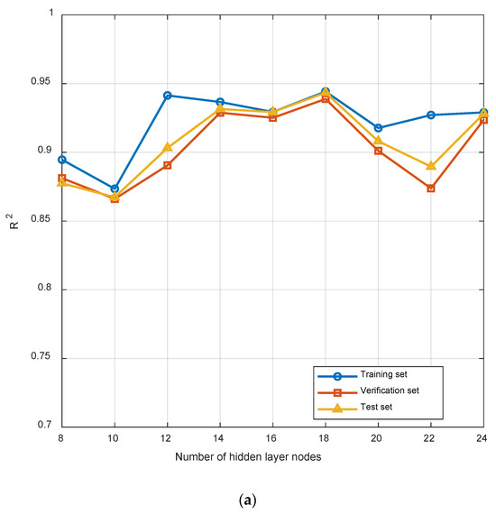
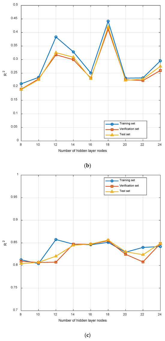
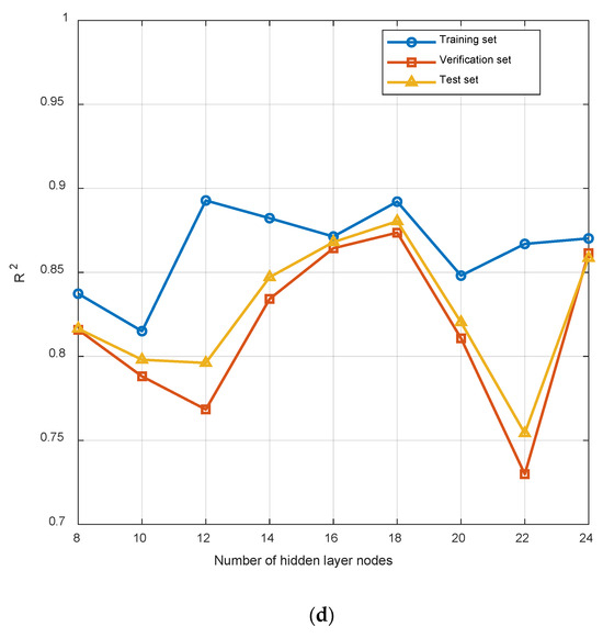
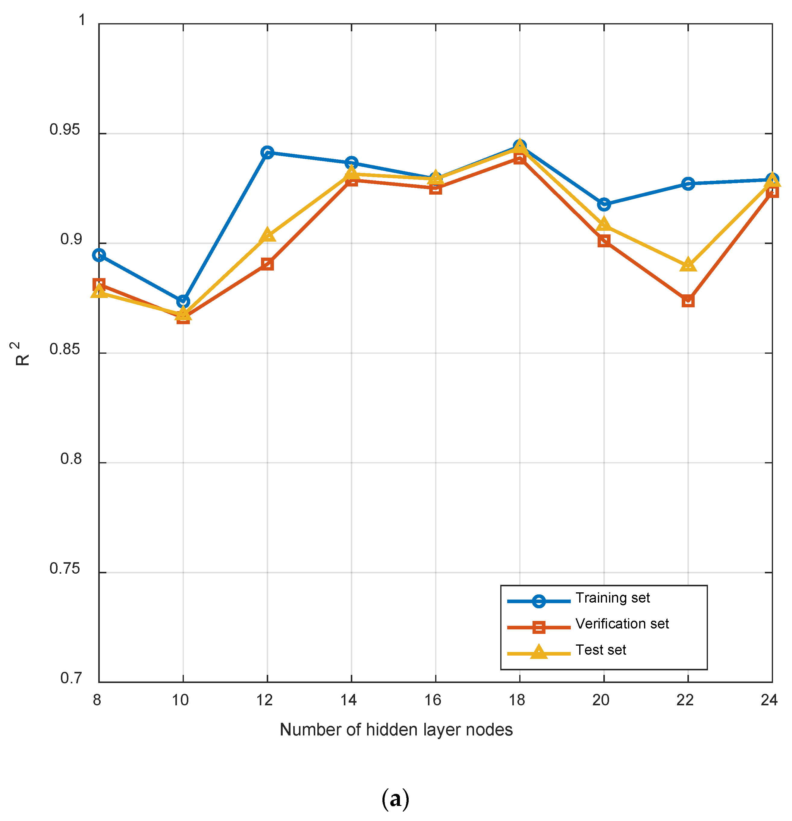
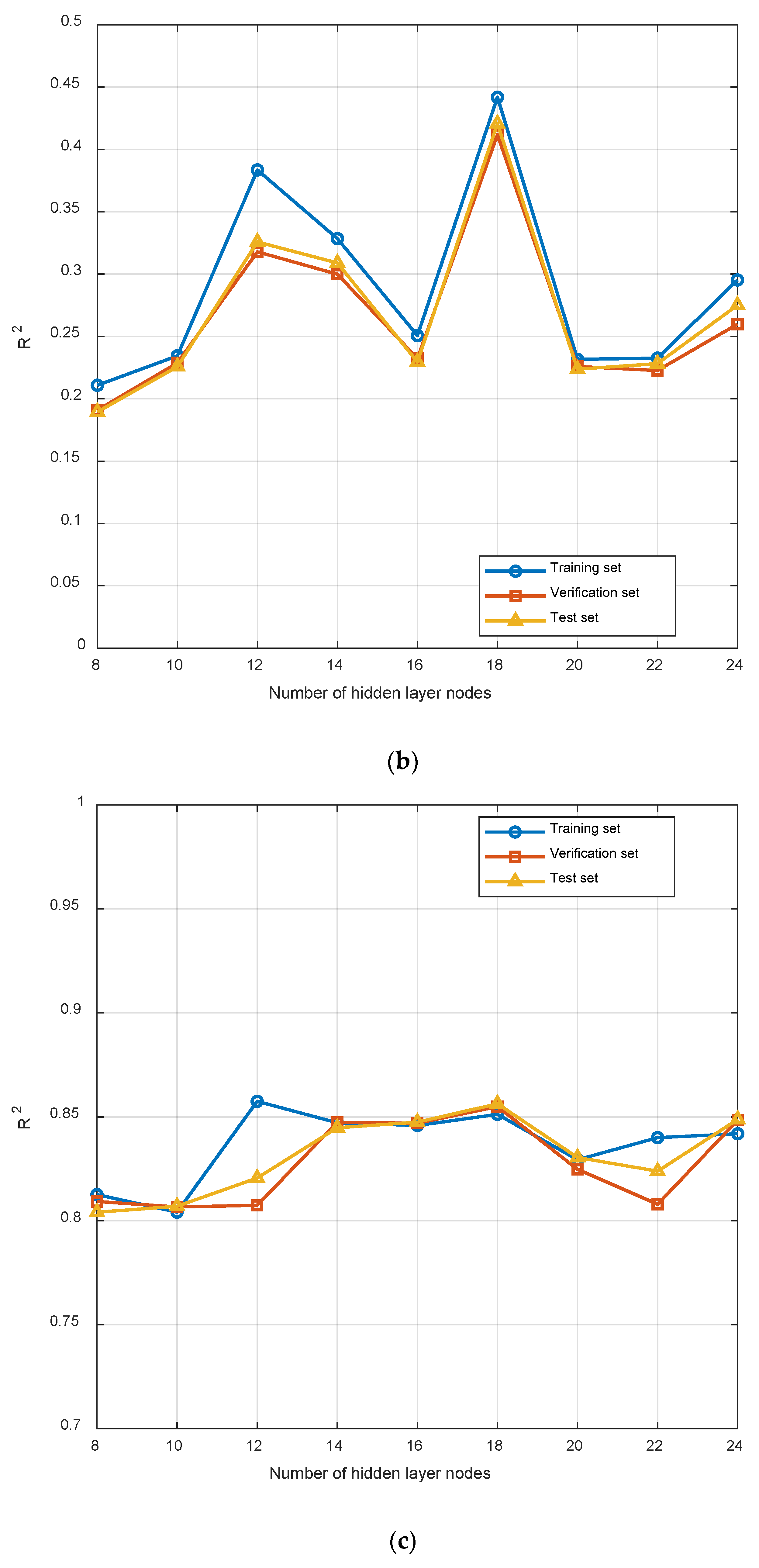
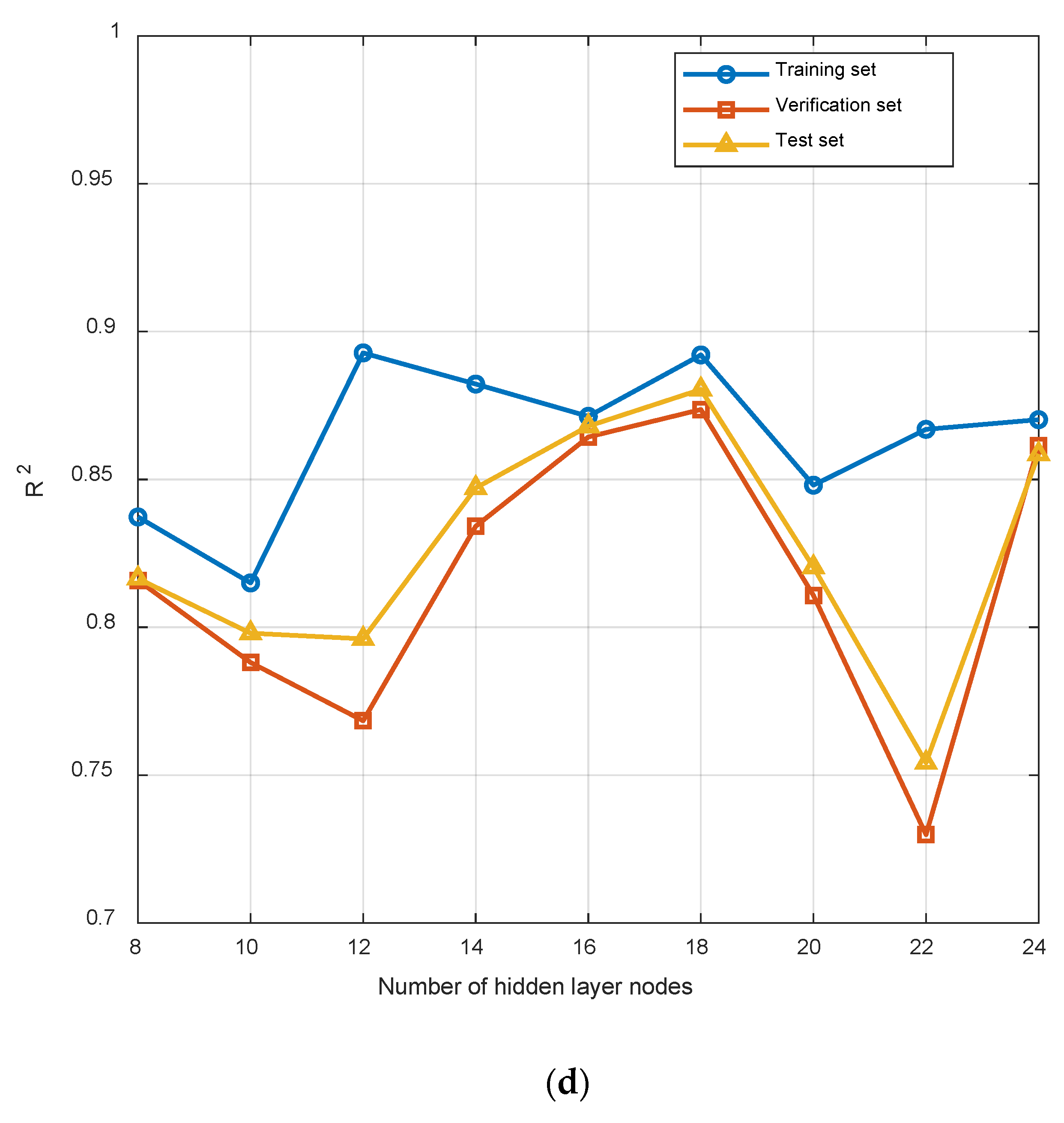
In neural networks, the number of nodes in the hidden layer is a crucial hyperparameter that directly determines the model’s capacity and its ability to generalize. Based on the available data, 18 nodes represent the most balanced and reliable choice (Figure 12).

Figure 12. (a) R² under different numbers of hidden layer nodes of furnace temperature; (b) R² under different numbers of hidden layer nodes of flue gas oxygen content; (c) R² under different numbers of hidden layer nodes of main steam flow; (d) R² under different numbers of hidden layer nodes of burnout point temperatures.

(2)

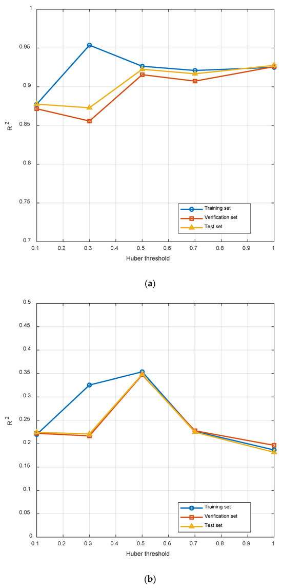
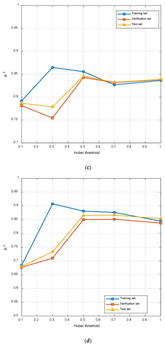
Huber threshold

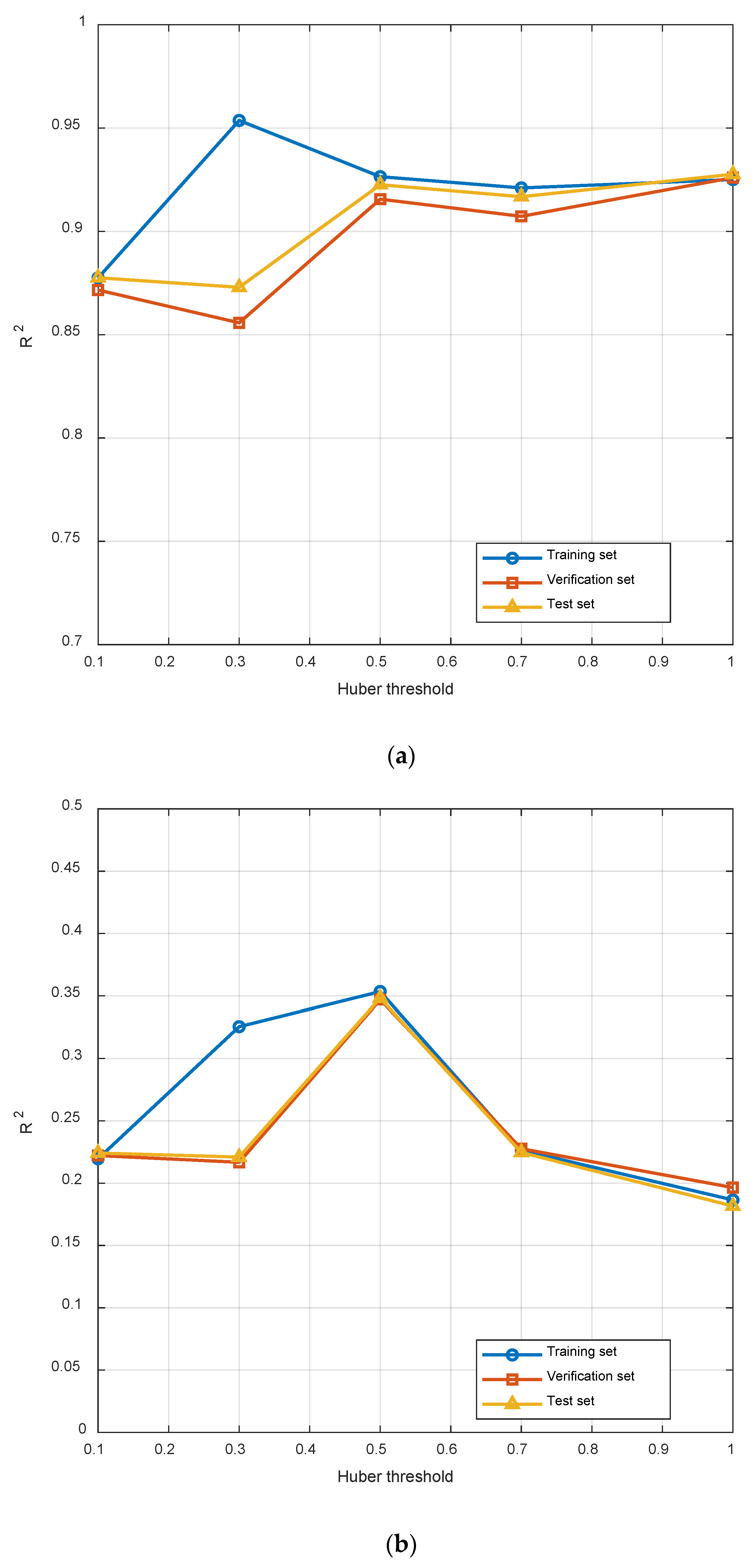
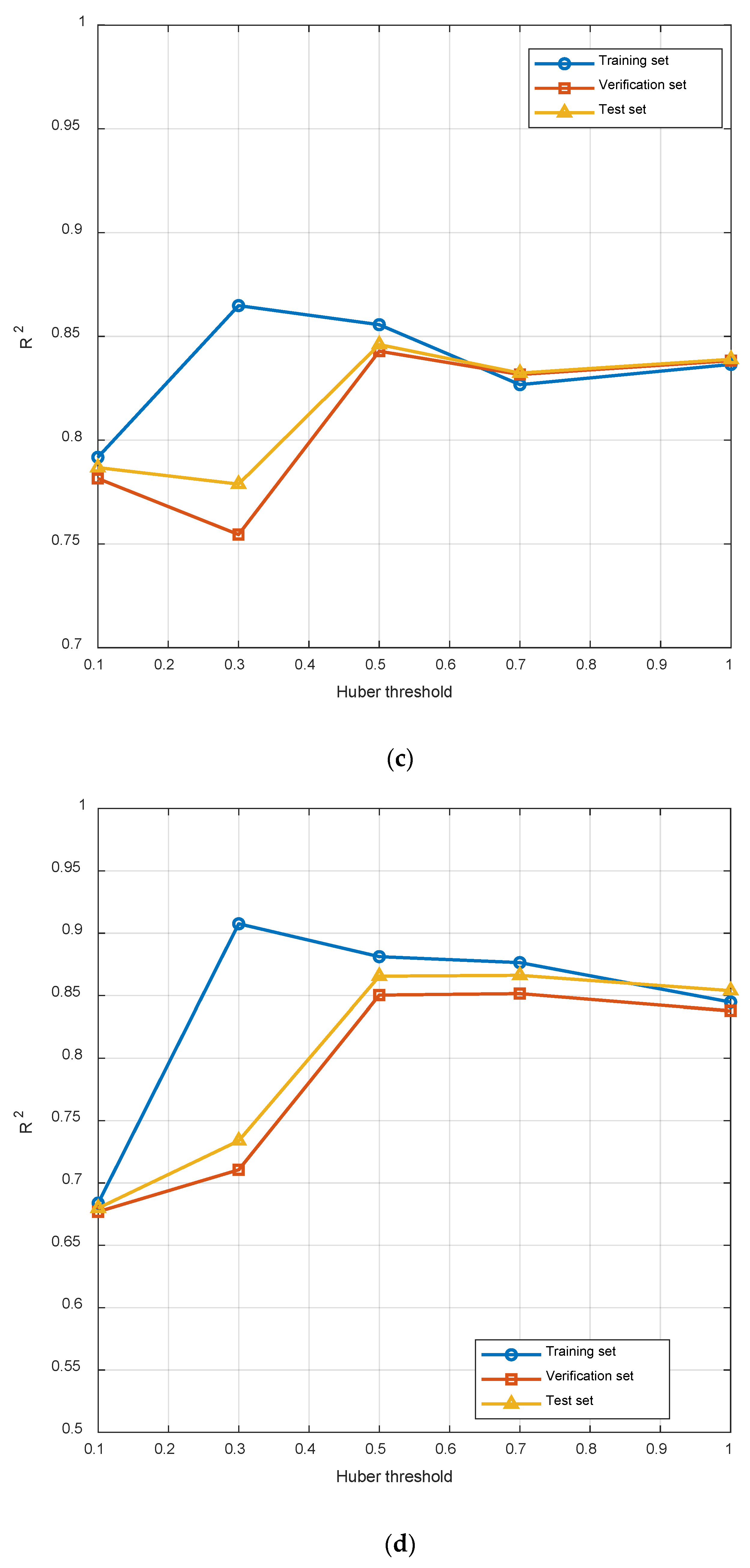
This parameter determines the model’s sensitivity and training stability regarding outliers in the data. By systematically comparing the model’s performance in terms of R² under different ${\theta }_{\delta }$ values, we can achieve a balance between training accuracy and the model’s generalization capability. This approach enables the selection of loss function parameters that best align with the characteristics of the current industrial process data, ensuring that the constructed model can not only accurately predict under normal working conditions but also handle data fluctuations in the production process with stability. A Huber Loss value of 0.5 may represent a more robust choice for effectively handling outliers in this context (Figure 13).

Figure 13. (a) R² under different Huber threshold nodes of furnace temperature; (b) R² under different Huber threshold nodes of flue gas oxygen; (c) R² under different Huber threshold nodes of main steam flow; (d) R² under different Huber threshold nodes of burnout point temperature.

(3)

Epochs

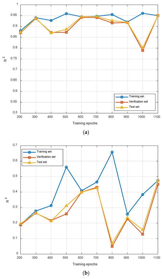
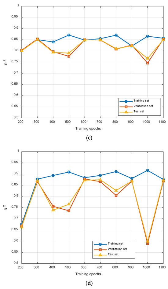
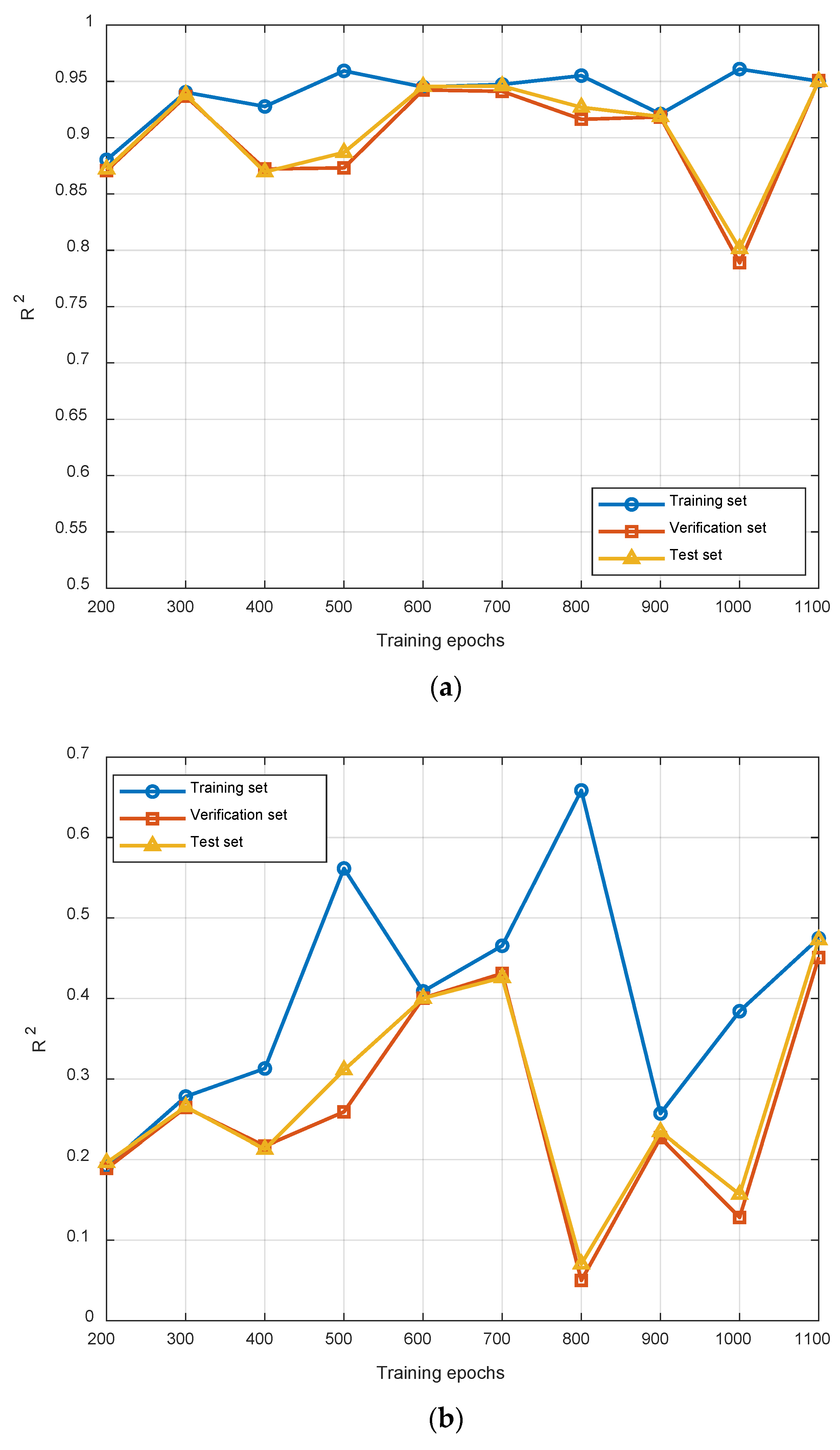
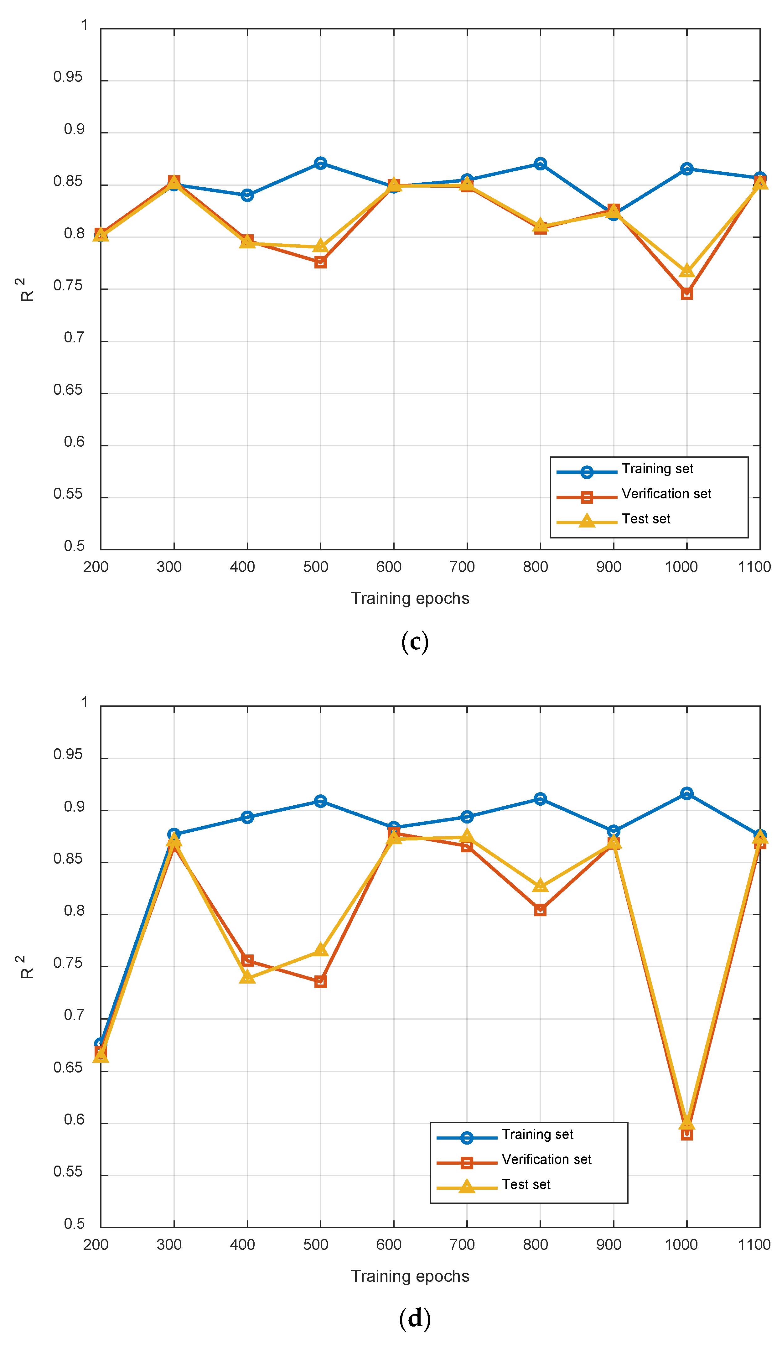
By adjusting the number of training epochs, the model weights are updated, resulting in improved prediction accuracy. Beginning with 200 training epochs, the number of epochs is incrementally increased to 1100 in increments of 100. The results are illustrated in the figure. The performance after 700 epochs is balanced and stable across several metrics, with minimal gaps between the validation set and the test set, indicating no significant overfitting. Consequently, 700 epochs yield the best overall performance (Figure 14).

Figure 14. (a) R² under different training epoch nodes of furnace temperature; (b) R² under different training epoch nodes of flue gas oxygen content; (c) R² under different training epoch nodes of main steam flow; (d) R² under different training epoch nodes of burnout point temperature.

(4)

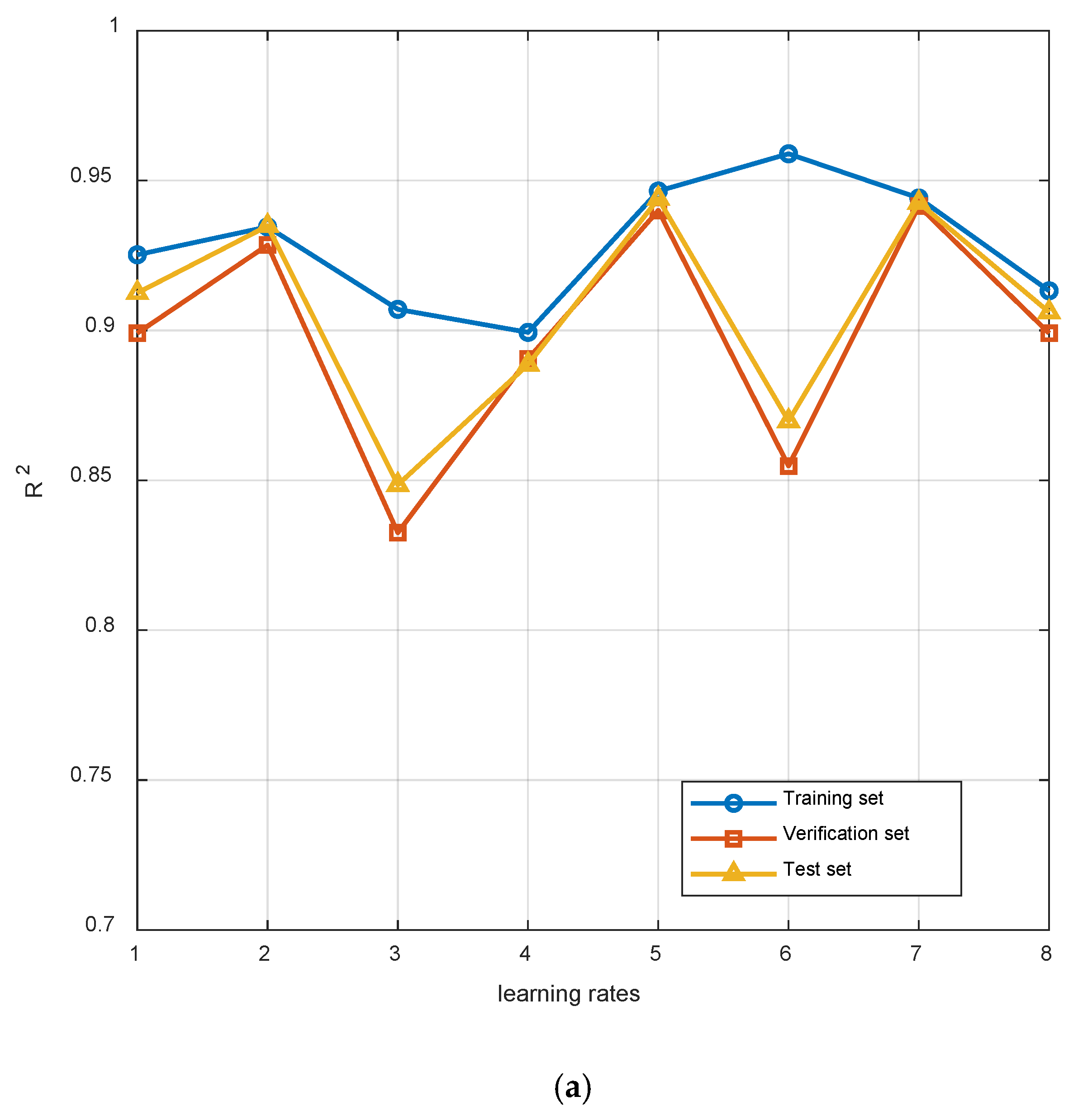
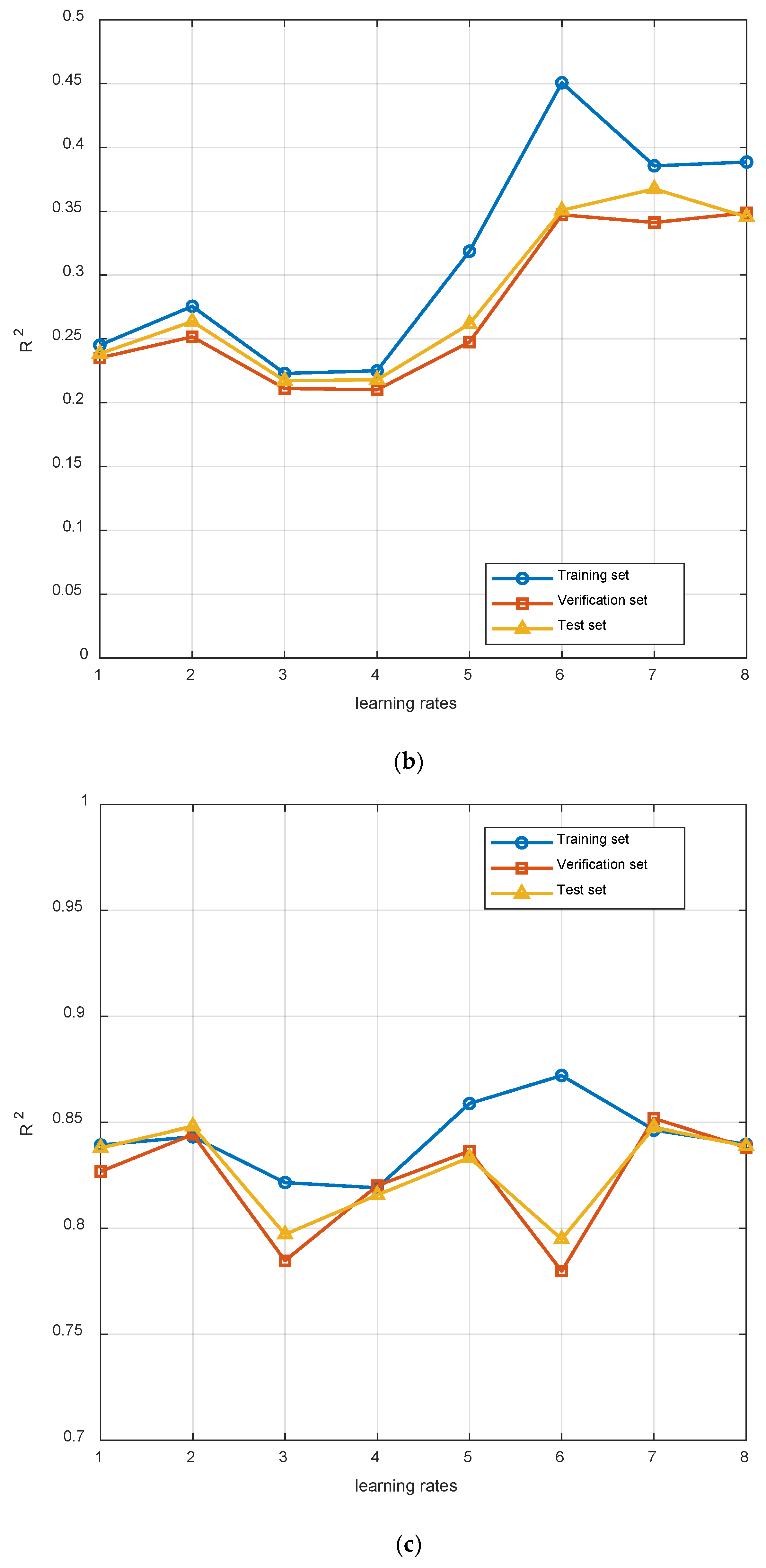
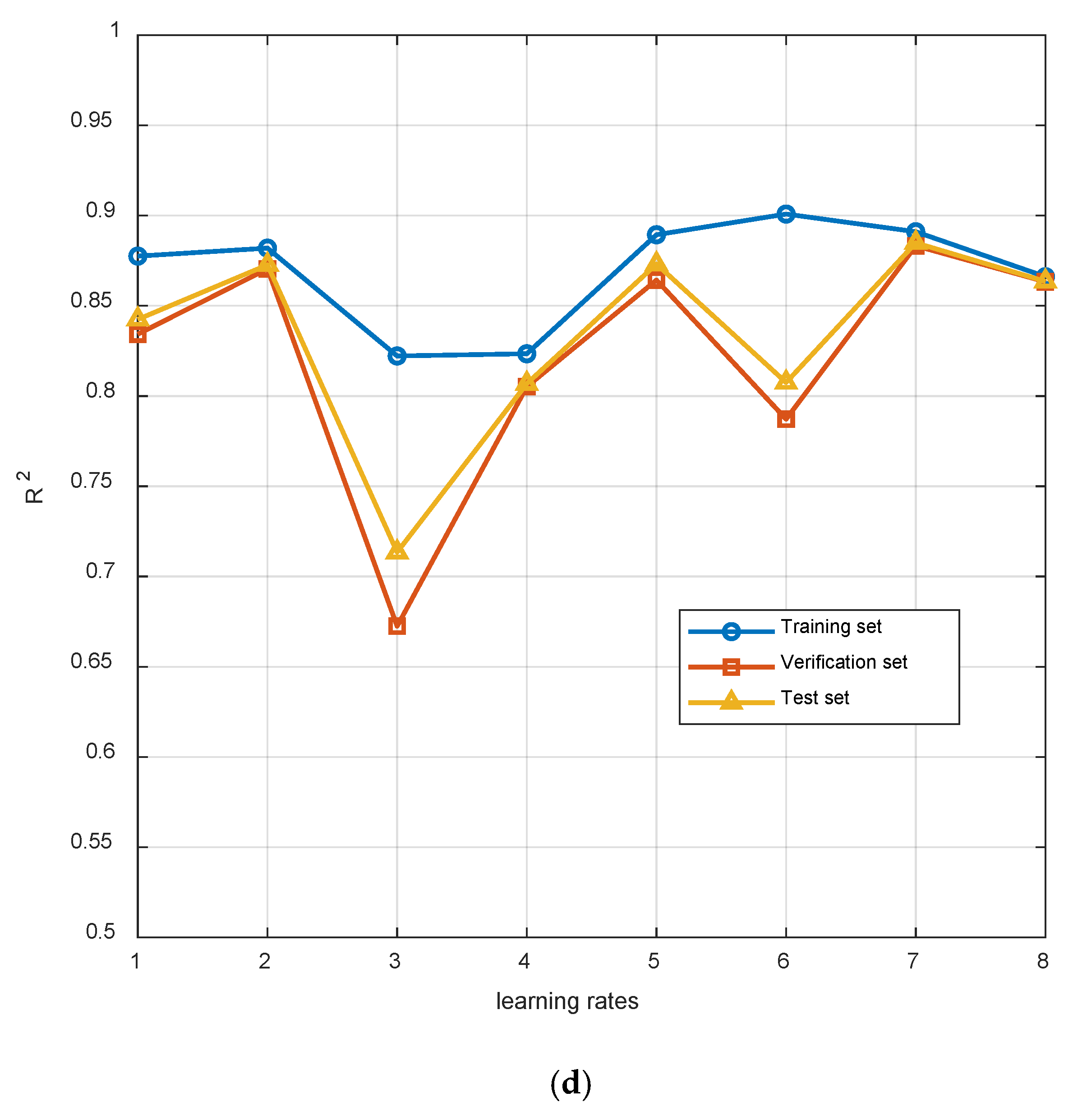
Learning rate

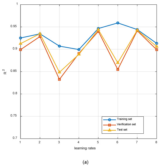
The learning rate critically influences the convergence speed, training stability, and generalization performance of neural networks. An excessively small learning rate (e.g., η = 0.0001) slows down convergence and increases the risk of being trapped in local optima. Conversely, an overly large learning rate may cause training instability and overfitting, leading to high training accuracy but poor generalization on validation and test sets.

As summarized in Table 9, experiments 1–4 examine the effect of progressively increasing ${\eta }_1$ while keeping ${\eta }_2$ and ${\eta }_3$ fixed at 0.0008. The results indicate that model performance improves steadily as ${\eta }_1$ increases, with the best trade-off achieved at ${\eta }_1$ = 0.001. Experiments 6–8 investigate the impact of simultaneously reducing ${\eta }_2$ and ${\eta }_3$ while maintaining ${\eta }_1$ = 0.001. Among these, the configuration with ${\eta }_2$ = ${\eta }_3$ = 0.0006 yields the most balanced performance across training, validation, and test sets.

Table 9. Learning rate combinations for hyperparameter analysis in Figure.

Experiment No.	(η1)	(η2)	(η3)	Description
1	0.0001	0.0008	0.0008	Varying η1, fixed η2/η3
2	0.0003	0.0008	0.0008	Varying η1, fixed η2/η3
3	0.0005	0.0008	0.0008	Varying η1, fixed η2/η3
4	0.0007	0.0008	0.0008	Varying η1, fixed η2/η3
5	0.001	0.001	0.001	All learning rates equal
6	0.001	0.0008	0.0008	Fixed η2/η3, η1 = 0.001
7	0.001	0.0006	0.0006	Fixed η1 = 0.001, varying η2/η3
8	0.001	0.0004	0.0004	Fixed η1 = 0.001, varying η2/η3

Based on the comprehensive analysis, the optimal learning rate combination is identified as ${\eta }_1$ = 0.001, ${\eta }_2$ = 0.0006, and ${\eta }_3$ = 0.0006. This setting demonstrates superior generalization ability and stability across all controlled experimental conditions (Figure 15).

Figure 15. (a) R² under different learning rates of furnace temperature; (b) R² under different learning rates of furnace temperature; (c) R² under different learning rates of main steam flow; (d) R² under different learning rates of burnout point temperature.

(5)

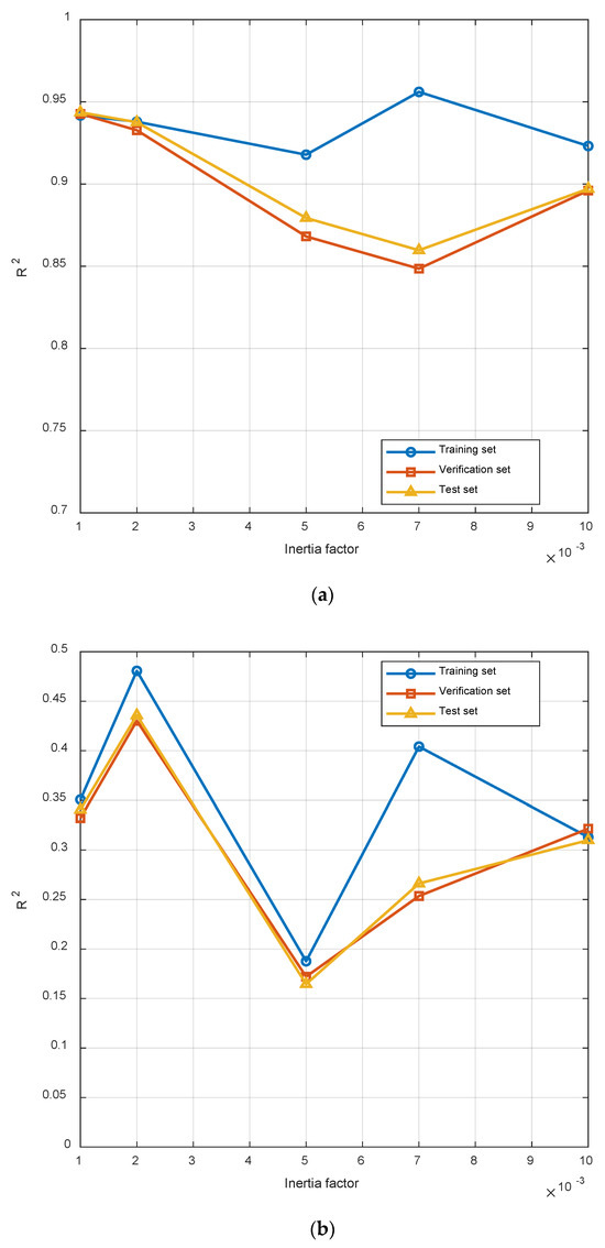
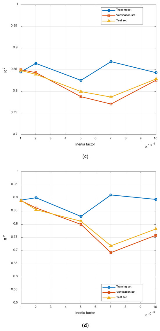
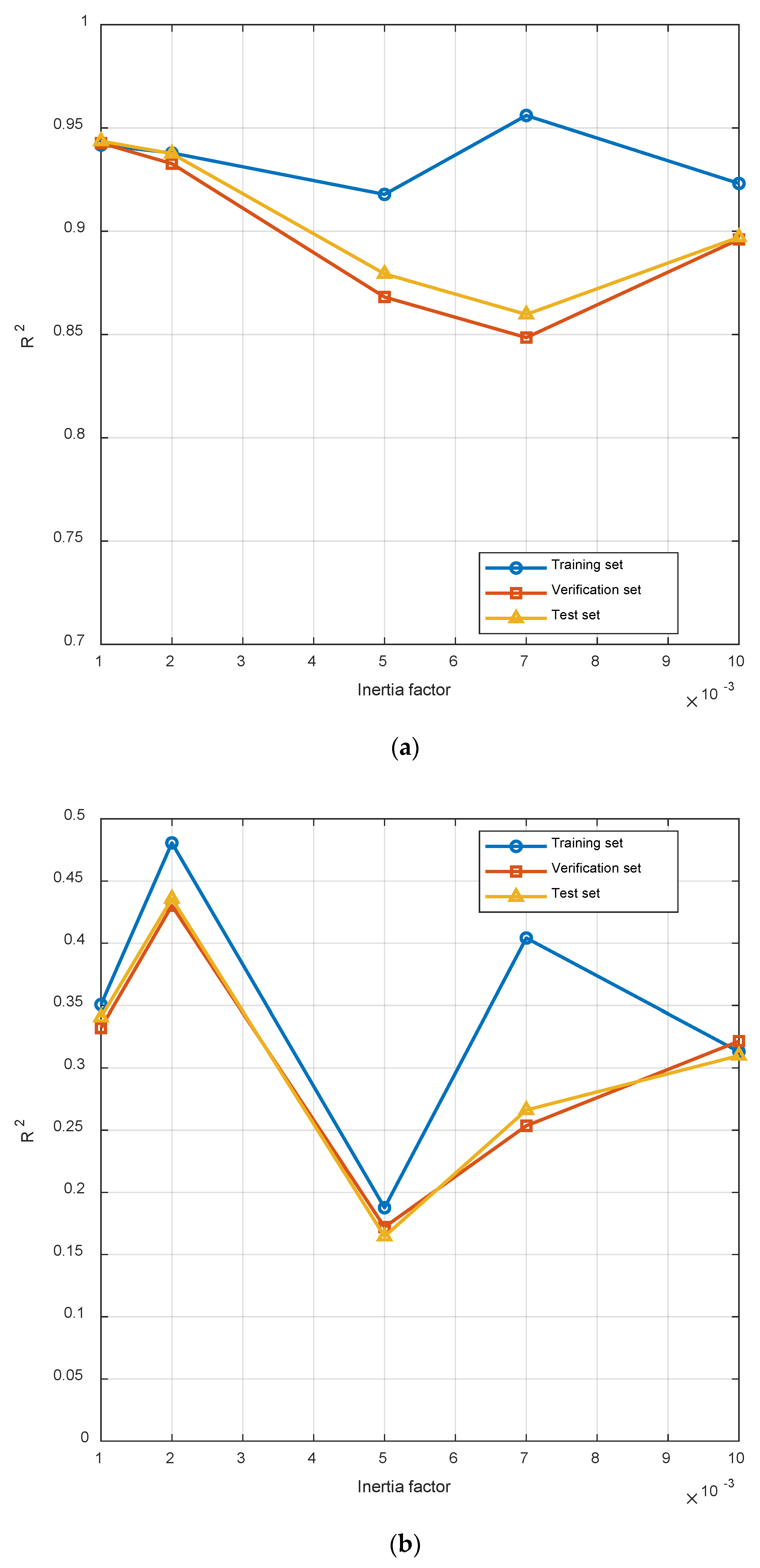
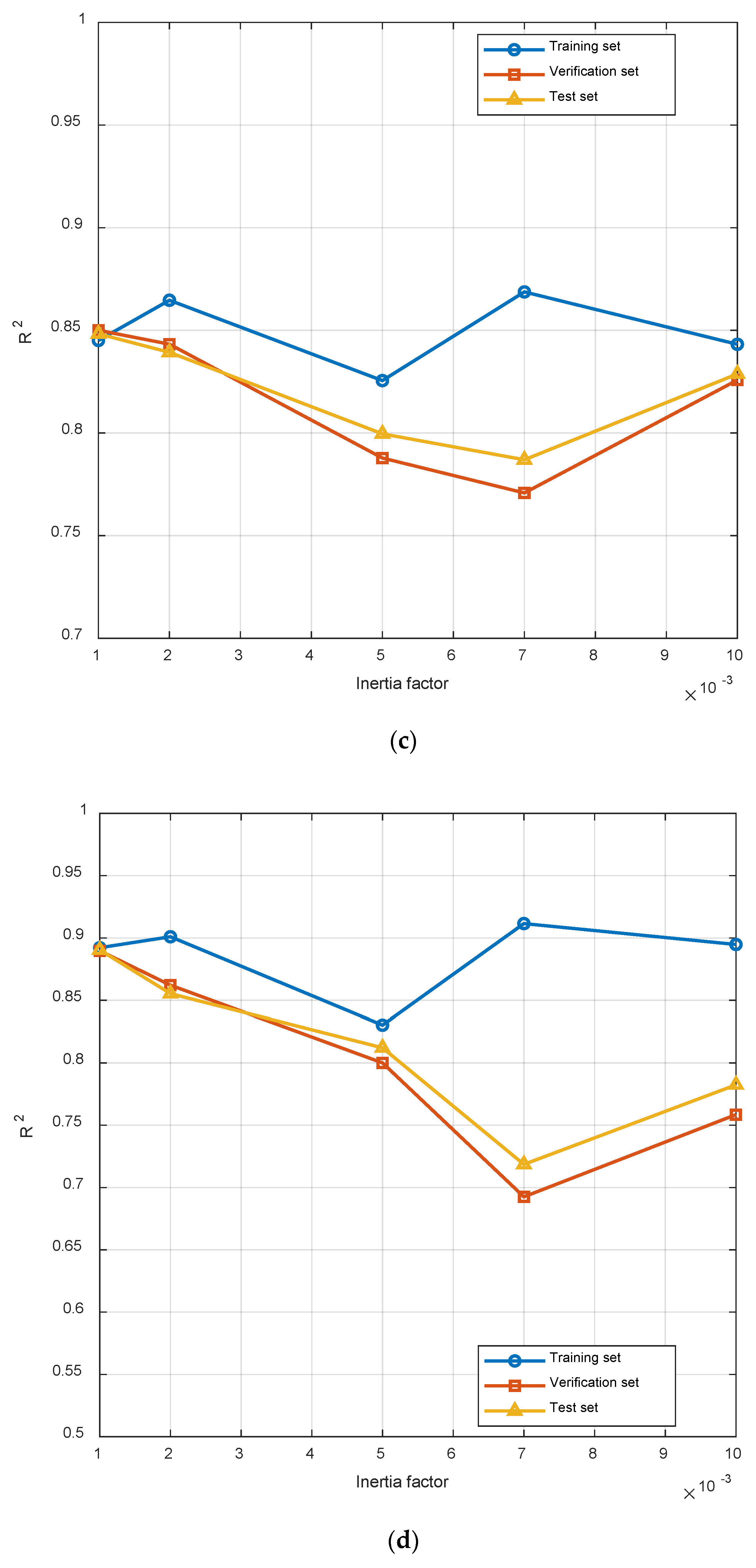
Inertia factor

The inertia factor is utilized in optimization algorithms (e.g., particle swarm optimization) to balance the model’s global search and local convergence capabilities. When the inertia factor is small, the model tends to concentrate on local fine-tuning and is susceptible to falling into local minima. When the inertia factor is large, the model tends to explore the search space globally; however, convergence may become challenging or lead to significant fluctuations. The optimal solution is identified as an inertia factor of 0.001, which provides robust generalization performance and stability while maintaining the system’s overall fitting accuracy, thereby rendering it suitable for practical control scenarios (Figure 16).

Figure 16. (a) R² under different inertia factors of furnace temperature; (b) R² under different inertia factors of flue gas oxygen content; (c) R² under different inertia factors of main steam flow; (d) R² under different inertia factors of burnout point temperature.

4. Conclusions

This study proposes a multi-controlled variable modeling method based on shared feature identification and an improved fuzzy neural network (Improved FNN), and systematically compares its performance with BPNN, RBFNN, and MIMO-TSFNN across four different datasets. Based on the experimental results, the following meaningful conclusions can be drawn. The improved FNN achieves the highest R² values and the lowest RRMSE values on almost all datasets. Particularly on the FT dataset, its training set R² reaches as high as 0.9355 with an RRMSE approaching zero, significantly outperforming other comparison models, which fully demonstrates its powerful capability in capturing complex nonlinear relationships. In terms of generalization performance, traditional models such as RBFNN exhibit significant performance degradation on the validation and test sets, whereas the improved FNN maintains highly consistent and excellent performance across the training, validation, and test sets, indicating that it not only possesses strong fitting ability but also exhibits superior generalization performance. When facing high-complexity datasets such as FGOC, although the performance of all models declines to varying degrees, the Improved FNN still maintains relatively optimal results, reflecting its strong robustness to data variability and noise. Furthermore, the standard deviations of R² and RRMSE across multiple experiments remain within small ranges, confirming that the Improved FNN has good stability and reliability, making it a trustworthy prediction tool for practical applications. Although the proposed multi-controlled variable modeling method has demonstrated its effectiveness and rationality through experimental data validation, we acknowledge that certain limitations exist in its practical application. When applied to different incineration facilities or varying operating conditions, the model’s generalization ability may be constrained due to differences in waste composition, equipment specifications, and environmental factors; meanwhile, the model’s adaptability to complex and variable operating conditions (such as fluctuations in municipal solid waste characteristics) still requires improvement. To address these limitations and advance the research, future work will focus on the following directions. First, promoting the transition from “prediction” to “control” by integrating the predictive model into a closed-loop optimization system to enable real-time control and decision support, thereby enhancing the model’s practical application value in dynamic industrial environments. Second, improving the model’s robustness and adaptability under complex and variable furnace conditions by introducing advanced techniques such as adaptive learning algorithms and real-time data assimilation, enabling it to better handle uncertainties and variations in operating conditions. Third, conducting large-scale validation across different incineration devices and facilities to comprehensively evaluate the model’s generalization performance and scalability. In summary, the ultimate goal of this research is to develop an intelligent control system that can be widely applied across various practical working conditions, contributing to environmental sustainability and the resolution of the “waste-besieged city” dilemma.

Although this study employs RRMSE, APE, and R² as the primary evaluation metrics—dimensionless indicators that facilitate cross-model comparisons—the following discussion converts these relative errors into absolute deviations with physical units to enhance engineering inter-reliability for practitioners. A comparative validation against the Improved FNN model is also provided:

(1)

Furnace temperature: The proposed model achieves a test set MAE of 5.32 °C, while the Improved FNN attains an R² of 0.9096 and an RRMSE approaching zero. Although the average deviation of 5.32 °C is slightly higher than that of the high-precision benchmark model, it remains sufficient to capture the dynamic variation of furnace combustion conditions (R² = 0.88), rendering it suitable for operational status monitoring and trend warning;

(2)

Flue gas oxygen content: The proposed model yields a test set MAE of 0.53%. In contrast, the Improved FNN exhibits a notably low R² of only 0.2714 on this variable, indicating poor goodness-of-fit. The prediction accuracy of 0.53% is close to the ±0.5% measurement error tolerance of industrial online analyzers, and significantly outperforms the benchmark model in terms of fitting effectiveness. This demonstrates clear engineering value for direct combustion optimization assistance;

(3)

Main steam flow: The proposed model achieves a test set MAE of 0.60 t/h, whereas the Improved FNN shows an R² of 0.8248 with an RRMSE near zero. The average deviation of 0.60 t/h surpasses the conventional accuracy requirement of ±1.0 t/h for thermal power control systems. Both models exhibit high-precision prediction levels suitable for direct engineering deployment.

(4)

Burnout point temperature: The proposed model attains a test set MAE of 4.53 °C, compared to the Improved FNN’s R² of 0.8233 and near-zero RRMSE. This prediction deviation falls within the ±5 °C allowable tolerance of industrial process control, and both models satisfy the engineering monitoring requirements for this measurement point.

In summary, the proposed Improved MIMO-FNN model achieves engineering-grade prediction accuracy for main steam flow, approaches industrial instrumentation and control requirements for flue gas oxygen content and burnout point temperature, and provides reliable trend references for furnace temperature. The method demonstrates distinct engineering advantages in the challenging task of flue gas oxygen content prediction, validating its comprehensive engineering applicability in multi-output prediction scenarios.

References

- Gómez-Sanabria, A.; Kiesewetter, G.; Klimont, Z.; Schoepp, W.; Haberl, H. Potential for Future Reductions of Global GHG and Air Pollutants from Circular Waste Management Systems. Nat. Commun. 2022, 13, 106. [Google Scholar] [CrossRef] [Scilit]
- Ali, K.; Kausar, N.; Amir, M. Impact of Pollution Prevention Strategies on Environment Sustainability: Role of Environmental Management Accounting and Environmental Proactivity. Environ. Sci. Pollut. Res. 2023, 30, 88891–88904. [Google Scholar] [CrossRef] [Scilit]
- Liu, J.; Zheng, L. Structure Characteristics and Development Sustainability of Municipal Solid Waste Treatment in China. Ecol. Indic. 2023, 152, 110391. [Google Scholar] [CrossRef] [Scilit]
- Yin, D.; Zhao, J.; Liu, J.-W.; Zhou, J.; Cheng, L.; Zhao, J. A Review of China’s Municipal Solid Waste (MSW) and Comparison with International Regions: Management and Technologies in Treatment and Resource Utilization. J. Clean. Prod. 2021, 293, 126144. [Google Scholar] [CrossRef] [Scilit]
- Raj, M.; Ghosh, A.; Ilame, T.; Kumar, S. Plastic Waste Management Strategies: Planning through Sustainable Lens and Way Forward towards Circular Economy. Discov. Sustain. 2025, 6, 361. [Google Scholar] [CrossRef] [Scilit]
- UNEP. Global Waste Management Outlook 2024; UNEP: Nairobi, Kenya, 2024. [Google Scholar]
- Yang, G.; Liu, M.; Gao, Y.; Han, S.; Meng, F.; Ju, T.; Jiang, J. A Review on the Evaluation Models and Impact Factors of Greenhouse Gas Emissions from Municipal Solid Waste Management Processes. Environ. Sci. Pollut. Res. 2024, 31, 27531–27553. [Google Scholar] [CrossRef] [Scilit] [PubMed]
- Kumar, A.; Singh, E.; Mishra, R.; Lo, S.L.; Kumar, S. Global Trends in Municipal Solid Waste Treatment Technologies through the Lens of Sustainable Energy Development Opportunity. J. Energy 2023, 275, 127471. [Google Scholar] [CrossRef] [Scilit]
- Rouhani, A.; Hejcman, M. A Review of Soil Pollution around Municipal Solid Waste Landfills in Iran and Comparable Instances from Other Parts of the World. Int. J. Environ. Sci. Technol. 2025, 22, 9711–9728. [Google Scholar] [CrossRef] [Scilit]
- Ayilara, M.S.; Olanrewaju, O.S.; Babalola, O.O.; Odeyemi, O. Waste Management through Composting: Challenges and Potentials. Sustainability 2020, 12, 4456. [Google Scholar] [CrossRef] [Scilit]
- Chu, X.; Jin, Y.; Wang, X.; Wang, X.; Song, X. The Evolution of the Spatial-Temporal Differences of Municipal Solid Waste Carbon Emission Efficiency in China. Energies 2022, 15, 3987. [Google Scholar] [CrossRef] [Scilit]
- Soni, A.; Gupta, S.K.; Rajamohan, N.; Yusuf, M. Waste-to-Energy Technologies: A Sustainable Pathway for Resource Recovery and Materials Management. J. Mater. Adv. 2025; in press. [CrossRef] [Scilit]
- Rahman, I.U.; Mohammed, H.J.; Bamasag, A. An Exploration of Recent Waste-to-Energy Advancements for Optimal Solid Waste Management. Discov. Chem. Eng. 2025, 5, 7. [Google Scholar] [CrossRef] [Scilit]
- Kaza, S.; Yao, L.; Bhada-Tata, P.; Van Woerden, F. What a Waste 2.0: A Global Snapshot of Solid Waste Management to 2050; World Bank: Washington, DC, USA, 2018; Available online: http://documents.worldbank.org/curated/en/697271544470229584 (accessed on 17 October 2025).
- Shen, W.; Zhu, N.; Xi, Y.; Huang, J.; Li, F.; Wu, P.; Dang, Z. Effects of Medical Waste Incineration Fly Ash on the Promotion of Heavy Metal Chlorination Volatilization from Incineration Residues. J. Hazard. Mater. 2022, 425, 128037. [Google Scholar] [CrossRef] [Scilit]
- Zhang, N.; Liu, W.; Li, J.; Liu, L.; Tan, Q. Quantifying Carbon Reduction Potential of “Zero-Waste City” Pilot: A Case Study of Shenzhen Based on Source Reduction-Recycling-Disposal Framework. J. Environ. Sci. 2025; in press. [CrossRef] [Scilit] [PubMed]
- Pian, J.; Si, M.; Sun, A.; Tang, J. Sustainability-Oriented Furnace Temperature Prediction for Municipal Solid Waste Incineration Using IWOA-SAGRU. Sustainability 2025, 17, 8987. [Google Scholar] [CrossRef] [Scilit]
- Li, X.; Ma, Y.; Zhang, M.; Zhan, M.; Wang, P.; Lin, X.; Chen, T.; Lu, S.; Yan, J. Study on the Relationship between Waste Classification, Combustion Condition and Dioxin Emission from Waste Incineration. Waste Dispos. Sustain. Energy 2019, 1, 91–98. [Google Scholar] [CrossRef] [Scilit]
- Wu, Q.; Xu, H. Intelligent Control Strategy of Incineration Process Pollution in Municipal Solid Waste. In Advances in Intelligent Systems and Computing; Cao, B.Y., Wang, P.Z., Liu, Z.L., Zhong, Y.B., Eds.; Springer: Cham, Switzerland, 2016; Volume 443, pp. 315–323. [Google Scholar] [CrossRef] [Scilit]
- Wang, Q.; Gong, D.; Huang, Z.; Peng, C.; Chen, J.; Luo, J.; Zhu, J.; Luo, Q. Simulation Study on the Stabilization Control Performance of Low-Calorific-Value Waste Combustion in Waste Incinerators. ACS Omega 2024, 9, 48586–48597. [Google Scholar] [CrossRef] [Scilit]
- Guo, M.R.; Zhang, B.R.; Xi, J.R.; Zhang, B. Physicochemical Properties and Heavy Metal Pollution Characteristics of Incineration Fly Ash before and after Refuse Classification. J. Environ. Eng. Technol. 2022, 12, 843–850. [Google Scholar] [CrossRef]
- Nghiem, T.X.; Drgoňa, J.; Jones, C.; Nagy, Z.; Schwan, R.; Dey, B.; Chakrabarty, A.; Di Cairano, S.; Paulson, J.A.; Carron, A.; et al. Physics-Informed Machine Learning for Modeling and Control of Dynamical Systems. In Proceedings of the 2023 American Control Conference (ACC), San Diego, CA, USA, 31 May–2 June 2023; IEEE: New York, NY, USA, 2023; pp. 3735–3750. [Google Scholar] [CrossRef] [Scilit]
- Zhuang, J.; Tang, J.; Aljerf, L. Comprehensive Review on Mechanism Analysis and Numerical Simulation of Municipal Solid Waste Incineration Process Based on Mechanical Grate. Fuel 2022, 320, 123826. [Google Scholar] [CrossRef] [Scilit]
- Quiñones-Grueiro, M.; Prieto-Moreno, A.; Verde, C.; Llanes-Santiago, O. Data-driven monitoring of multimode continuous processes: A review. Chemom. Intell. Lab. Syst. 2019, 189, 16. [Google Scholar] [CrossRef] [Scilit]
- Wang, T.; Tang, J.; Xia, H.; Yang, C.; Yu, W.; Qiao, J. Data-Driven Multi-Objective Intelligent Optimal Control of Municipal Solid Waste Incineration Process. Eng. Appl. Artif. Intell. 2024, 137, 109157. [Google Scholar] [CrossRef] [Scilit]
- Guyon, I.; Elisseeff, A. An Introduction to Variable and Feature Selection. J. Mach. Learn. Res. 2003, 3, 1157–1182. Available online: https://dl.acm.org/doi/10.5555/944919.944968 (accessed on 21 November 2025).
- Cui, B.C.; Wang, X.X.; Zhou, B.M.; Tan, H.; Xiong, X. Experimental study on the gasification-combustion characteristics and nox emission characteristics of pulverized coal. Electr. Power Technol. Environ. Prot. 2024, 40, 133–141. [Google Scholar] [CrossRef]
- Huang, K.; Wen, H.; Ji, H.; Cen, L.; Chen, X.; Yang, C. Nonlinear Process Monitoring Using Kernel Dictionary Learning with Application to Aluminum Electrolysis Process. Control Eng. Pract. 2019, 89, 94–102. [Google Scholar] [CrossRef] [Scilit]
- Liang, L.; Sun, R.; Fei, J.; Wu, S.; Liu, X.; Dai, K.; Yao, N. Experimental Study on Effects of Moisture Content on Combustion Characteristics of Simulated Municipal Solid Wastes in a Fixed Bed. Bioresour. Technol. 2008, 99, 7238–7246. [Google Scholar] [CrossRef] [Scilit]
- Tang, J.; Tian, H.; Yu, W.; Qiao, J. A Review of Neural Network Control in Municipal Solid Waste Incineration Processes. Acta Autom. Sin. 2025, 51, 1951–1973. [Google Scholar] [CrossRef]
- Gao, X.Q.; Yang, F.; Shang, C.; Huang, D.X. A Review of Control Loop Monitoring and Diagnosis: Prospects of Controller Maintenance in Big Data Era. Chin. J. Chem. Eng. 2016; in press. [CrossRef] [Scilit]
- Peterson, L.; Gosea, I.V.; Benner, P.; Sundmacher, K. Digital Twins in Process Engineering: An Overview on Computational and Numerical Methods. Comput. Chem. Eng. 2025, 193, 108917. [Google Scholar] [CrossRef] [Scilit]
- Guo, J.; Yin, X.; Yan, A. Furnace Temperature Prediction Model in Municipal Solid Waste Incineration Process Based on Slow Feature Analysis and Sparse Stochastic Configuration Network. Eng. Appl. Artif. Intell. 2025, 162, 112701. [Google Scholar] [CrossRef] [Scilit]
- Sun, J.; Meng, X.; Qiao, J. Prediction of Oxygen Content Using Weighted PCA and Improved LSTM Network in MSWI Process. IEEE Trans. Instrum. Meas. 2021, 70, 2507512. [Google Scholar] [CrossRef] [Scilit]
- Zhao, Z.; Zhou, Z.; Lu, Y.; Li, Z.; Wei, Q.; Xu, H. Predictions of the Key Operating Parameters in Waste Incineration Using Big Data and a Multiverse Optimizer Deep Learning Model. Sustainability 2023, 15, 14530. [Google Scholar] [CrossRef] [Scilit]
- Chen, L.; Zheng, L.; Xie, Y.; Gao, X.; Lin, Y.; Yu, Z.; Lai, L. Characteristics and Kinetics of the Co-Pyrolysis of Oil Shale and Municipal Solid Waste Assessed via Thermogravimetric Analysis. Sustainability 2026, 18, 753. [Google Scholar] [CrossRef] [Scilit]
- Ding, H.; Tang, J.; Xia, H.; Qiao, J.F. Modeling of MIMO Controlled Object in Municipal Solid Waste Incineration Process Based on TS-FNN. Control Theory Appl. 2022, 39, 1529–1540. Available online: https://link.cnki.net/urlid/44.1240.TP.20220311.0956.002 (accessed on 18 October 2025).
- Takagi, T.; Sugeno, M. Fuzzy Identification of Systems and Its Applications to Modeling and Control. IEEE Trans. Syst. Man Cybern. 1985, 15, 116–132. [Google Scholar] [CrossRef] [Scilit]
- Tapkir, A. A Comprehensive Overview of Gradient Descent and its Optimization Algorithms. Int. Adv. Res. J. Sci. Eng. Technol. 2023, 10, 37–45. [Google Scholar] [CrossRef] [Scilit]
- Wang, Q.; Ma, Y.; Zhao, K.; Tian, Y. A Comprehensive Survey of Loss Functions in Machine Learning. Ann. Data. Sci. 2022, 9, 187–212. [Google Scholar] [CrossRef] [Scilit]
Disclaimer/Publisher’s Note: The statements, opinions and data contained in all publications are solely those of the individual author(s) and contributor(s) and not of MDPI and/or the editor(s). MDPI and/or the editor(s) disclaim responsibility for any injury to people or property resulting from any ideas, methods, instructions or products referred to in the content. |
© 2026 by the authors. Licensee MDPI, Basel, Switzerland. This article is an open access article distributed under the terms and conditions of the Creative Commons Attribution (CC BY) license.