A Stacking-Based Multi-Step LSTM and Policy-Enhanced SVR Method for Carbon Emission Prediction

Abstract

China’s “dual-carbon” targets require more scientifically precise methods for carbon emission forecasting. Existing methods mainly rely on time series or regression models: the former captures temporal trends but lacks interpretability, while the latter provides explanatory power but struggles with nonlinear patterns. To overcome these limitations, this paper applies a multi-step LSTM with transfer learning to capture nonlinear temporal dynamics of carbon emissions, incorporates an SVR with added policy variables to improve accuracy, and finally employs a stacking model to integrate above advantages. Predictions are then aggregated via linear regression to leverage complementary strengths. The proposed model is trained on 1960–2004 data and tested on 2005–2019, 2023 and 2024 data. Results show that the optimized LSTM and SVR improve prediction accuracy, while the Stacking-based ensemble surpasses individual models in accuracy and robustness. Based on the integrated model, predictions for 2023–2050 indicate that if policies are strengthened in 2025, China’s carbon emissions will peak in 2024 and subsequently decline to about 8175 Mt CO₂ by 2050; if policies are not strengthened in 2025, emissions will peak in 2026 and subsequently decline to about 6983 Mt CO₂.

1. Introduction

In recent years, carbon emissions, a key driver of global climate change, have drawn significant international attention. The IPCC Sixth Assessment Report warns that without effective mitigation, global surface temperatures could rise by 2.4–4.4 °C by century’s end, profoundly affecting ecosystems, public health, and economic development. These impacts directly threaten the environmental, economic, and social pillars of sustainable development, undermining long-term global sustainability. According to statistics released by the World Bank, China has remained the largest annual CO₂ emitter since the mid-2000s, accounting for roughly one-third of global emissions in recent years, while its emission growth rate has gradually moderated alongside structural economic transformation and energy transition policies. Against this backdrop, China announced its “dual-carbon” goals at the 75th UN General Assembly in 2020—peaking emissions by 2030 and achieving neutrality by 2060. These goals have since been incorporated into top-level strategies, including the Outline of the 14th Five-Year Plan, marking the start of a systematic low-carbon transition. This transition represents a critical pathway for China to align economic growth with ecological protection and to advance sustainable development at the national level.

Following the announcement of the “dual-carbon” goals, China has made significant strides in renewable energy deployment, green finance, and regulation of energy-intensive industries. Yet, structural constraints—such as a carbon-intensive industrial composition, reliance on high-carbon energy, and regional imbalances—continue to pose substantial challenges for achieving emission reductions. Accurately forecasting carbon emission trajectories, identifying key mitigation pathways, and systematically evaluating policy impacts have become central task to China’s green transition and sustainable development. Reliable emission forecasting is essential for designing effective long-term mitigation strategies, optimizing resource allocation, and ensuring that emission reduction efforts support economically viable and socially equitable sustainable development outcomes. In this context, developing a forecasting model tailored to China not only supports the achievement of peak carbon and neutrality targets but also offers significant theoretical and practical insights for high-quality development and ecological governance. Moreover, such models provide quantitative decision support for integrating climate objectives into broader sustainable development planning.

In the field of carbon emission forecasting and analysis, researchers both domestically and internationally have proposed various models and approaches, mainly including time series models, regression analysis, and multi-method ensemble models. These studies have made significant progress in expanding methodological tools and improving predictive accuracy, yet each approach still exhibits distinct limitations. From a sustainability perspective, limitations in model interpretability, robustness, and policy relevance may weaken their ability to guide long-term low-carbon transitions and sustainable policy formulation. In the domain of traditional time series models, researchers predominantly exploit historical data to extract patterns in carbon emissions. Alam et al. (2025) proposed the CarbonMLP model with XAI methods to forecast transportation emissions using Canadian vehicle data, achieving high accuracy and identifying key drivers, but with dependence on historical data completeness and limited interpretability [1]. Wang et al. (2025) employed a discrete second-order difference equation coupled with a BP neural network to predict peak emissions for smart buildings, effectively capturing historical trends and improving forecast accuracy, yet the model does not account for external factors such as policy or technological changes and thus has limited adaptability [2]. Liu et al. (2024) used a particle swarm optimization (PSO) grey prediction model combined with a metabolic algorithm to forecast carbon emissions in China’s construction sector, revealing regional disparities and growth trends; while short-term forecasts are accurate, the grey model’s long-term reliability is limited [3]. Hou et al. (2024) applied a Bayesian-optimized XGBoost model to panel data from seven coastal regions (2005–2020) to predict construction sector emissions, accurately identifying population, GDP, and completed construction area as principal drivers and achieving high predictive performance, though the model’s effectiveness depends on the completeness of input features [4]. In regression-based approaches, researchers have increasingly incorporated multidimensional drivers and complex models to enhance explanatory power. Wang et al. (2023) implemented a two-stage forecasting framework that integrates Support Vector Regression (SVR) with multiple machine learning models, including random forest, ridge regression (RR), and artificial neural networks, achieving high-precision CO₂ emission forecasts; however, the model’s structural complexity increases interpretability challenges, and reliance on cross-model assumptions limits robustness [5]. Chen et al. (2024) applied grey relational analysis to select key factors influencing emissions in the logistics sector, followed by PSO to tune SVR parameters, thereby constructing a high-accuracy forecasting model for China’s logistics emissions; despite improved predictive precision, the approach increases model complexity and demands high-quality input data [6]. In contrast, Zhong et al. (2022) used a logistic curve model to analyze Jiangsu Province’s emission trajectory by setting an S-shaped relationship between urban expansion and cumulative emissions; while the model is simple and intuitive for fitting emission caps and inflection points during urban growth, it heavily relies on maximum capacity assumptions and the stability of historical trends, limiting its ability to capture policy or technological shocks [7]. Rao et al. (2023), based on an extended STIRPAT model combined with RR and scenario analysis, revealed the elastic effects of population, economy, energy, and industrial structure on Hubei Province’s emissions, providing clear scenario pathways and strong policy relevance, yet the approach still falls short in terms of describing nonlinear effects and handling external uncertainties such as sudden policies or extreme events [8]. Similarly, Zhang et al. (2025) developed an interpretable machine learning-based forecasting framework that integrates ensemble regression techniques with SHapley Additive exPlanations (SHAPs) to predict CO₂ emissions and reveal key driving factors in university campus emissions scenarios; however, the model still faces inherent limitations owing to residual machine learning “black box” characteristics and its dependency on historical training data, constraining its capacity to generalize across diverse spatial contexts and support robust long-term policy analysis [9]. Conversely, Xie et al. (2025) employed the LEAP energy system model to simulate sector- and energy-specific emission pathways in the Sichuan–Chongqing region, offering strong systemic and policy-oriented insights, yet the model heavily depends on parameter settings and expert assumptions, limiting its capacity to capture nonlinear dynamic changes [10]. To address the aforementioned limitations, multi-method fusion models have emerged to balance predictive accuracy and policy relevance. Liu and Zheng (2025), based on the Kaya identity combined with scenario analysis, simulated carbon emission pathways for Changning City, Hunan Province (2022–2031); their scenario design is clear and policy-relevant but remains limited in addressing spatial heterogeneity and external uncertainties [11]. Feng et al. (2023) applied the LEAP energy system model, the Kaya identity, and LMDI decomposition at the firm level, combined with scenario analysis to produce sector-specific forecasts for industrial emissions and to propose mitigation pathways; this approach offers comprehensive accounting and clear structure with strong policy orientation [12]. Zhang (2025) developed a hybrid short-term carbon emission forecasting framework that combines complete ensemble empirical mode decomposition with adaptive noise (CEEMDAN), empirical wavelet transform (EWT) denoising, and long short-term memory (LSTM) networks to enhance signal feature extraction and predictive accuracy; however, its decomposition complexity and residual dependence on historical emission sequences still limit policy scenario analysis and generalization across varied emission contexts [13]. Zhang et al. (2025) employed an improved back propagation neural network optimized via the Improved Sparrow Search Algorithm (ISSA) to develop a high-precision CO₂ emission forecasting model for the civil aviation sector, achieving enhanced accuracy; however, the model still exhibits inherent limitations due to retaining machine learning “black box” characteristics and its dependency on historical training data, which constrain its transparency and capacity for policy scenario analysis [14]. Although these fusion models enhance predictive performance, further improvements are needed to ensure their applicability for long-term sustainability planning and policy evaluation.

In summary, despite progress in modeling carbon emissions, several limitations remain. Single time series models struggle to capture nonlinear dynamics and lack stability, while regression models offer interpretability but insufficiently incorporate policy variables and complex interactions. AI methods provide strong predictive performance yet often function as “black boxes” with limited policy interpretability. By explicitly linking emission forecasting with policy evaluation, this framework provides actionable insights for low-carbon transition pathways and supports evidence-based decision-making for sustainable development. Ensemble models typically employ simple integration, neglecting deep fusion and variable expansion. In sum, statistical models are transparent but inadequate for nonlinear dynamics and policy shocks, whereas machine learning and system models improve accuracy at the expense of complexity, opacity, and data dependency. Enhancing both interpretability and robustness, systematically integrating policy variables, and advancing multi-model optimization remain urgent challenges.

Building on the above observations, the present study develops an integrated forecasting framework for China’s carbon emissions, combining time series and multivariate regression approaches. Multi-step LSTM networks, optimized via Bayesian methods, capture nonlinear temporal dynamics, while SVR incorporating policy variables quantifies the effects of population, economy, and energy. A Stacking ensemble then integrates the strengths of both models, improving predictive accuracy, robustness, and interpretability. This approach addresses limitations of single-model methods—including lack of policy consideration and insufficient optimization—providing scientific evidence and policy insights to support China’s peak carbon and neutrality targets. Ultimately, the proposed framework contributes to balancing economic growth, environmental protection, and social welfare, thereby advancing China’s long-term sustainable development goals.

2. Data Description

This study uses China’s carbon emission data from 1960 to 2024, obtained from the Global Carbon Atlas [15]. Data on other influencing factors are sourced from the China Statistical Yearbook and China Energy Statistical Yearbook (National Bureau of Statistics). Definitions of the main variables are presented in Table 1.

Table 1. Description of Variables.

Variable	Definition	Unit	Mean	Var	Min	Max
C	Carbon emissions	Mt	5384	11,511,869	1476	11,350
P	Population size	10,000 persons	124,703	167,301,698	98,705	141,260
A	Per capita GDP	10,000 CNY/person	2.68	5.68	0.30	8.02
E	Energy intensity	t/10,000 CNY	0.99	0.19	0.48	2.05
S	Energy structure	%	91.88	13.63	82.50	96.00
U	Urbanization rate	%	39.79	208.88	19.39	65.22

3. Methodology

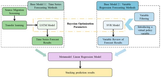
This study develops a machine learning–based framework for carbon emission forecasting using a multi-model stacking ensemble. LSTM networks capture temporal dependencies in emission data through a multi-step forecasting strategy, thereby reducing error accumulation inherent in recursive predictions. SVR captures nonlinear relationships and abrupt changes in emission data. Input data are preprocessed differently for each base learner—normalized for LSTM and standardized for SVR—and hyperparameters are optimized via Bayesian Optimization (BO) to improve robustness. Out-of-fold predictions generated through time series cross-validation serve as inputs for a linear regression meta-learner, which integrates the strengths of both base models while maintaining interpretability. This LSTM-SVR stacking ensemble effectively combines temporal patterns with feature information, enhancing predictive accuracy, robustness, and interpretability. The overall framework of this study is illustrated in Figure 1, where the green blocks represent base model 1 (LSTM), the blue blocks denote base model 2 (SVR), and the purple block corresponds to the meta-model. The dashed frame indicates the optimization algorithm (BO).

Figure 1. Flowchart of the proposed Stacking integrated carbon emission forecasting framework.

3.1. Time Series Forecasting Methods

Since traditional linear forecasting methods exhibit limitations in modeling multivariate inputs and capturing long-term dependencies, deep learning approaches have increasingly become the mainstream in time series forecasting in recent years. As an improved architecture of RNNs, LSTM network introduces gating mechanisms such as the “forget gate” within its units, effectively alleviating problems of gradient vanishing and gradient explosion. This enables the LSTM to better characterize long-term dependency features in time series. With this advantage, LSTM demonstrates strong fitting capacity and generalization performance in multi-input and multi-step forecasting tasks, and has been widely applied in diverse fields including financial markets, energy system modeling, and macroeconomic forecasting [16].

However, the time series spanning 1960–2024 remains insufficient for effectively training an LSTM model, limiting its capability in parameter learning and generalization under small-sample conditions. To address this issue, a VMD–DTW framework is first employed to quantitatively evaluate long-term trend similarity among national carbon emission series and to identify potential source countries with evolution patterns highly consistent with China. Subsequently [17], an LSTM model is pretrained via transfer learning using the selected source domains and then fine-tuned with Chinese data, thereby improving the stability and predictive accuracy of carbon emission forecasting in the target region [18].

3.1.1. Normalization of Time Series Data

In time series forecasting, the differences in scales and magnitudes across various indicators may significantly affect both the convergence speed and the prediction accuracy of the model. To eliminate the influence of heterogeneous scales and improve training stability, this paper applies the Min–Max normalization method to the raw data, mapping the series to the interval [0, 1]:

$$x_{\mathrm{norm}}={\displaystyle \frac{x-x_{min}}{x_{max}-x_{min}}},$$

where, $x$ denotes the original observation, while $x_{min}$ and $x_{max}$ represent the minimum and maximum values observed in the selected test set of the series, respectively.

3.1.2. Trend Similarity Analysis and Selection of Transfer Learning Source Domains

To quantitatively assess the trend similarity of carbon emission time series across countries and identify suitable source domains for transfer learning, this study first applies Variational Mode Decomposition (VMD) to the carbon emission sequences. Let the original sequence be $x\left(t\right)$; by setting the number of modes $K=4$ and the penalty parameter $\alpha =2000$, the sequence is decomposed into several intrinsic mode functions (IMFs), with the lowest-frequency IMF selected as the principal component representing long-term trends. To eliminate the influence of heterogeneous emission magnitudes on similarity measurements, the Min–Max normalization method is applied, mapping the trend sequences of China and other countries separately to the interval [0, 1], which preserves the variation intrinsic to China while ensuring cross-country scale consistency.

Based on trend extraction and normalization, the Dynamic Time Warping (DTW) distance is employed to construct a similarity matrix among countries, and hierarchical clustering is used to reveal the grouping structure of global carbon emission patterns. For source domain selection in transfer learning, countries are classified into strong, medium, and low similarity categories according to the quantiles of DTW distances relative to China. Strongly similar countries are chosen as primary source domains, medium-similarity countries as auxiliary sources, and low-similarity countries are excluded. This approach establishes a complete quantitative framework from trend decomposition, scale normalization, similarity measurement, to source domain selection, providing a reliable basis for transfer learning in cross-country carbon emission forecasting.

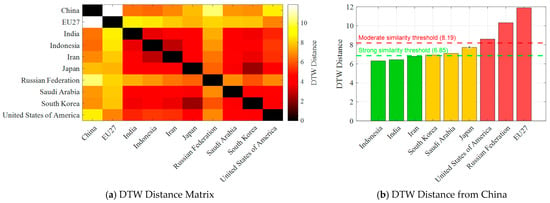
Building upon the aforementioned methodology, this study further systematically evaluates the feasibility of transfer learning between China and other major economies. The DTW distance quantitatively characterizes temporal pattern similarity, where smaller values indicate higher dynamic consistency and greater potential for effective knowledge transfer. As shown in Figure 2, Indonesia, India, and Iran exhibit strong similarity to China, while the DTW distances of South Korea, Saudi Arabia, and Japan are all below the strong-similarity threshold (6.85), indicating highly consistent temporal evolution patterns. Accordingly, strongly similar economies are selected as primary source domains, and moderately similar ones are employed as auxiliary source domains.

Figure 2. DTW Distance Analysis of Regional Time Series.

3.1.3. LSTM Modeling with Transfer Learning

The core workflow of the transfer learning-based LSTM is as follows: historical carbon emission data from China and nine representative countries are collected and normalized using the Min–Max method to ensure cross-country scale consistency. Sequences of length five are constructed from the other countries’ data to pretrain the LSTM model, capturing general emission patterns. The network consists of a sequence input layer, a 64-unit LSTM hidden layer, two fully connected layers with ReLU activation, and a regression output layer. After pretraining, 70% of China’s data are used to fine-tune the model, with the final fully connected layer replaced and assigned higher learning rates to adapt to China-specific features. The remaining data are reserved for validation, and predictive performance is evaluated using MAE, RMSE, and MAPE. The fine-tuned model is then applied for multi-step forecasting from 2025 to 2050, with residuals bootstrapped to quantify uncertainty and construct 95% confidence intervals. For clarity, the training and multi-step forecasting procedure of the transfer learning-based LSTM is described below.

Algorithm 1 presents a transfer learning LSTM framework for multi-step prediction of China’s carbon emissions. Historical emissions from China and nine representative countries are normalized and segmented into input–output sequences. The LSTM is pretrained on other countries’ data to capture general patterns, then fine-tuned on Chinese data with the last fully connected layer adjusted for local features. Validation metrics (MAE, RMSE, MAPE) assess model performance. The fine-tuned model performs rolling forecasts for future years, with bootstrap resampling applied to quantify uncertainty and construct 95% confidence intervals.

Algorithm 1 China’s Carbon Emissions Using Transfer Learning LSTM

Require: Historical Carbon Emissions Data E(t), Prediction Horizon nfuture Ensure: Forecasted Carbon Emissions for Future Years $\widehat{E}$(t) 1: Read carbon emissions time series $E\left(t\right)$ for all countries from the data file. 2: Separate China data $E_{\mathrm{China}}\left(t\right)$ and other countries’ data $E_{\mathrm{Others}}\left(t\right)$. 3: Normalize $E_{\mathrm{China}}\left(t\right)$ and $E_{\mathrm{Others}}\left(t\right)$ using Min–Max scaling. 4: Set sequence length $n_{\mathrm{Step}}=5$ and transfer ratio $r=0.7$. 5: Split China data: $E_{\mathrm{China},\mathrm{transfer}}=70\mathrm{\%}$, $E_{\mathrm{China},\mathrm{val}}=30\mathrm{\%}$ Pretraining on other countries’ data: 6: Construct sequences $\left(X_{\mathrm{pretrain}},Y_{\mathrm{pretrain}}\right)$ from $E_{\mathrm{Others}}\left(t\right)$. 7: Define LSTM network: sequence input → 64-unit LSTM → FC + ReLU → FC + ReLU → FC → regression output. 8: Train network using Adam optimizer with preset hyperparameters to obtain pretrain_net. Fine-tuning on China data: 9: Construct sequences $\left(X_{\mathrm{finetune}},Y_{\mathrm{finetune}}\right)$ from $E_{\mathrm{China},\mathrm{transfer}}\left(t\right)$. 10: Replace last fully connected layer of pretrain_net with new layer for China task, assign higher learning rate factors. 11: Fine-tune network using Adam optimizer to obtain finetune_net. Validation: 12: Construct validation sequences $\left(X_{\mathrm{val}},Y_{\mathrm{val}}\right)$ from $E_{\mathrm{China},\mathrm{val}}\left(t\right)$. 13: Predict $Y_{\mathrm{val},\mathrm{pred}}$ using finetune_net and inverse normalize. 14: Compute validation metrics: MAE, RMSE, MAPE. Multi-step prediction (2025–2050): 15: Construct sequences from full China data for final training. 16: Continue training finetune_net to obtain final_net. 17: Initialize last observed sequence, perform rolling prediction for $n_{\mathrm{future}}$ years to obtain $\widehat{E}\left(t\right)$. 18: Denormalize predictions. Uncertainty quantification via Bootstrap: 19: Compute residuals on training data. 20: Repeat $n_{\mathrm{bootstrap}}$ times: a. Resample residuals. b. Add to predicted outputs to generate bootstrap targets. c. Retrain network on bootstrap samples. d. Perform rolling prediction to obtain bootstrap forecast. 21: Compute 95% confidence intervals from bootstrap predictions. Output: 22: Visualize historical, predicted, and confidence intervals. 23: Save forecast table with point predictions and 95% CI. 24: Compute key indicators: peak year, peak emission, 2050 change. 25: Compare performance with model trained using only China data.

3.2. Variable Regression Forecasting Methods

Since the data used in this study cover only the period from 1980 to 2024, yielding a total of 44 samples, the sample size is relatively limited. Considering that SVR exhibits strong nonlinear modeling capability and robust generalization performance in small-sample settings, SVR is selected in this study as the tool for variable regression to characterize the relationships between various influencing factors and carbon emissions [16].

3.2.1. Data Standardization

Before training the SVR model, all input features are standardized to have zero mean and unit variance by

$$x_i^{\prime }={\displaystyle \frac{x_i-\mu }{\sigma }}.$$

where, $x_i$ represents the original feature value, $\mu$ and $\sigma$ denote the mean and standard deviation of this feature obtained from the selected test set, respectively, and $x_i^{\prime }$ is the standardized feature value.

This preprocessing is essential for SVR, as the model relies on kernel functions and weight optimization, making it sensitive to feature scale disparities. Standardization transforms features to zero mean and unit variance, preventing dominance of large-magnitude variables, ensuring balanced kernel computations, and thereby improving both convergence efficiency and predictive accuracy.

3.2.2. Selection of Influencing Factors and Introduction of Policy Dummy Variables

Previous studies have demonstrated that five factors—population size, economic development level, urbanization rate, energy intensity, and energy structure—exert significant impacts on carbon emissions [19]. For the purpose of quantitative analysis, this study adopts the year-end total population to represent population size, per capita GDP to reflect the level of economic development, and the gross industrial output value as a measure of energy intensity. Meanwhile, the share of fossil fuels in primary energy consumption is employed to characterize the energy structure, while the urbanization level is depicted by the proportion of urban permanent residents.

To facilitate model tractability and long-term forecasting, this study first assumes that the effects of policy interventions identified during the historical period can be linearly extrapolated into the forecast horizon, implying that the marginal impacts of policies on both the emission level and growth trend remain stable over time. Such an assumption is commonly adopted in long-term emission forecasting studies under data availability constraints.

To ensure that this linear extrapolation is grounded in empirically identifiable regime dynamics, the study further embeds endogenous structural breakpoint detection within a unified analytical framework that combines statistical identification with institutional interpretation. Structural breakpoints are detected using the Bai–Perron multiple structural breakpoint test, which accommodates unknown numbers and locations of regime shifts by minimizing the segmented sum of squared residuals (SSR) and employing sequential F-statistic testing. Robust parameter settings are adopted, including a minimum segment length of 10% of the sample size, a maximum of four allowable breakpoints, and a requirement that each segment contains at least 15% of total observations.

Empirical analysis of China’s carbon emission series from 1960 to 2024 identifies five statistically significant structural breakpoints—1969, 1980, 1992, 2002 and 2013—indicating multiple transitions in the underlying emission regime. Among these, the 2002 breakpoint produces the largest SSR reduction and the most significant F-statistic, implying a pronounced transformation in emission dynamics. To maintain consistency with the long-term linear extrapolation assumption while preserving institutional interpretability, representative structural turning points are ultimately defined at 1980, 1992, 2002, and 2013, corresponding respectively to the initiation of the national energy conservation policy framework, the establishment of the socialist market economy system, China’s accession to the World Trade Organization, and the transition to the “new normal” stage of economic development.

Based on these regime divisions, policy-related dummy variables $D$, capturing discrete level shifts, and post-break trend variables $T$. Their formal mathematical definitions are presented in Equations (1) and (2), respectively [20,21].

$$D_t=\sum _{j=1}^{4}1\left(t\ge {\mathrm{\tau }}_j\right),$$

(1)

$$T_t=\sum _{j=1}^4\left(t-{\mathrm{\tau }}_j\right)\hspace{0.17em}1\left(t\ge {\mathrm{\tau }}_j\right),$$

(2)

where, $1(\cdot )$ denotes the indicator function, and ${\mathrm{\tau }}_1=1980$, ${\mathrm{\tau }}_2=1992$, ${\mathrm{\tau }}_3=2002$, ${\mathsf{\tau }}_4=2013$.

The former reflects the level shift after the breakpoint, while the latter characterizes the change in the growth trend of carbon emissions. It should be noted that no additional scaling coefficients are introduced when constructing the policy dummy variables and policy trend variables. This is because all variables are standardized prior to model estimation, and the standardization process eliminates dimensional differences and absorbs the effects of scale. As a result, scaling coefficients no longer carry independent economic meaning in the estimation. To avoid parameter redundancy and maintain model parsimony, no separate scaling terms are specified for these policy variables.

3.2.3. SVR Modeling

SVR predicts target values and controls errors by constructing an optimal hyperplane in a high-dimensional feature space. Slack variables and a regularized loss function are introduced to optimize the model, while the kernel function enables efficient handling of nonlinear mappings. In this study, the RBF kernel is employed to enhance predictive accuracy and generalization [22]. For clarity, the training and prediction process of the SVR model is described in the following.

Algorithm 2 demonstrates that the prediction process primarily consists of the following stages: data preprocessing, SVR model training, historical data fitting, and multi-step forecasting. In the data preprocessing stage, historical carbon emission data and related influencing factors are standardized to eliminate differences in measurement scales and accelerate model convergence. During model training, the SVR model is trained using the full sample data, with hyperparameters (such as the penalty factor, epsilon, and kernel scale) optimized to enhance the model’s fitting capability. In the historical data fitting stage, the trained model is employed to predict the known series, thereby evaluating its ability to reproduce historical patterns. Finally, in the multi-step forecasting stage, the trained SVR model is applied to the explanatory variable series of the prediction period to estimate future carbon emissions.

Algorithm 2 Carbon Emissions Forecasting Based on SVR

Require: Historical emissions data E(t), explanatory variables X(t) Ensure: Future prediction $\widehat{E}$ future(t) 1:    Load E(t) and X(t) from dataset 2:    Apply normalization 3:    Split dataset into training and testing sets 4:    if Use Bayesian optimization then 5:             Define SVR hyperparameter search space: {C, ε, γ} 6:             Perform Bayesian optimization to obtain optimal parameters 7:    else 8:             Train SVR model with predefined parameters 9:    end if 10: Train final SVR model on the full training data 11: Fit historical data to obtain $\widehat{E}$ train(t) and apply inverse normalization 12: Perform multi-step prediction using Xfuture(t) 13: Inverse normalize results to obtain $\widehat{E}$ future(t)

3.3. Bayesian Optimization

BO is a probabilistic, model-based method for efficiently tuning hyperparameters of black box functions. It builds a prior over the objective function and iteratively updates the posterior using observed data to identify optimal hyperparameters without exhaustive search. In this study, BO is employed to tune the key hyperparameters of different models:

Optimized Hyperparameters for the LSTM Model

• Number of Hidden Units (N): Denotes the number of neurons in the LSTM hidden layer, determining the model’s expressive capacity and complexity. Larger values can capture more complex temporal dependencies but may lead to overfitting and increased computational cost.
• Initial Learning Rate (I): Controls the step size for parameter updates. A learning rate that is too high may prevent convergence, whereas a too-small learning rate may slow down the training process.
• Time Steps (n_step): Refers to the size of the input sequence sliding window, which determines the temporal range that the model can trace during prediction, thereby affecting its ability to capture long-term dependencies.
• Mini-Batch Size (MinSize): Indicates the number of samples used to update weights in each iteration. Smaller batches help capture finer fluctuations in the data, while larger batches improve training stability and efficiency.

Optimized Hyperparameters for SVR

• Penalty Factor (C): Balances model complexity and error penalty. A larger C emphasizes precise fitting of the training samples but may lead to overfitting, whereas a smaller C enhances generalization at the risk of underfitting.
• Insensitive Loss Parameter (ε): Defines the permissible deviation between predicted and true values. Prediction errors within this range are not penalized, enhancing the model’s robustness to noisy data.
• Kernel Scale (γ): Determines the width of the Radial Basis Function (RBF) kernel. A larger γ makes the model more sensitive to local features but may overfit, whereas a smaller γ emphasizes global patterns, producing a smoother model.

3.4. Stacking Ensemble Learning Framework

Ensemble learning is a class of methods that construct a stronger predictive model by combining the capabilities of multiple base learners, aiming to overcome the limitations of individual models and improve overall predictive accuracy and generalization. Common ensemble learning techniques include Stacking, Bootstrap Aggregating (Bagging), and Boosting [23]. In this study, Stacking is employed to build the carbon emission forecasting model. The core idea is to use the predictions of multiple base learners as new feature inputs, which are then fed into a meta-learner to generate the final prediction. Compared with a single model, Stacking can fully exploit the differences in performance of base learners across various features or data patterns, thereby achieving complementary advantages and enhancing both model robustness and predictive performance.

In this study, LSTM and SVR are selected as base learners, with Linear Regression (LR) serving as the meta-learner. The reasons for this structural design are as follows:

• LSTM Model [24]: LSTM captures long-term dependencies and nonlinear dynamics. This study employs multi-step forecasting, with Bayesian Optimization tuning hyperparameters to improve accuracy, stability, and prevent overfitting.
• SVR Model [25]: SVR constructs a maximum-margin hyperplane for strong generalization. Introducing a time breakpoint variable captures structural shifts in carbon emissions, while RBF kernels handle nonlinearities, making SVR suitable for small-sample, complex data.

In this study, Linear Regression is employed as the meta-learner to integrate the outputs of the base learners. The main reasons for selecting Linear Regression are as follows:

• Suitable for scenarios with weak multicollinearity: When base learner predictions are weakly correlated, Linear Regression reliably estimates their weights without regularization, reducing bias [26].
• Balanced model interpretability and efficiency: Linear Regression is simple and efficient, with coefficients that directly reflect base learner contributions, facilitating interpretation and application [27].

4. Results and Discussion

To evaluate model performance, error analysis was conducted, for which a reasonable test set partition is a critical prerequisite. The testing period was defined as 2005–2024. Given that 2020–2022 were subject to strong exogenous shocks from a public health emergency, during which carbon emissions exhibited abnormal fluctuations inconsistent with the intrinsic evolution of the economy–energy system, these three years were excluded from the core evaluation to avoid distortion of predictive performance. Accordingly, model validation was performed using 17 effective test years (2005–2019 and 2023–2024), which constitute the evaluation set for the subsequent error analysis.

4.1. Evaluation of Time Series Model Performance

To systematically evaluate the effectiveness of the transfer learning strategy for China’s carbon emission forecasting, a comparative experiment was conducted between the China-only LSTM model and the transfer learning–based model with cross-country pretraining and fine-tuning under a unified data partition. Consequently, model validation was performed using 17 effective test years, and the corresponding error statistics are summarized in Table 2.

Table 2. Comparison of Multi-Step and Single-Step Prediction Errors.

Method	MAE	RMSE	MAPE (%)	R2
China-only	448.53	554.08	4.53	0.8089
Transfer learning	381.66	470.98	3.83	0.8130

As shown in Table 2, the transfer learning model consistently outperforms the China-only model across major accuracy metrics. Specifically, MAE decreases from 448.53 to 381.66 Mt CO₂ (−14.9%), RMSE declines from 554.08 to 470.98 Mt CO₂ (−15.0%), and MAPE is reduced from 4.53% to 3.83%. Meanwhile, the goodness-of-fit R² improves from 0.8089 to 0.8130, indicating enhanced overall fitting stability alongside reduced prediction bias. These findings suggest that, under the constraint of limited availability and insufficient scale of China’s historical carbon emission data, single-country training is inadequate for robust deep temporal learning. In contrast, cross-country pretraining followed by China-specific fine-tuning effectively mitigates small-sample overfitting and improves the reliability of medium- to long-term trend estimation, demonstrating the superiority of the transfer learning framework for long-horizon carbon emission forecasting.

4.2. Evaluation of Variable Regression Models

In carbon emission forecasting research, traditional models typically rely on macroeconomic and energy indicators as explanatory variables for regression modeling [16]. However, such variables often fail to fully capture the impacts of structural shifts or institutional shocks on carbon emissions. To address this limitation, this study innovatively introduces the dummy variables D and T into the benchmark model, aiming to better characterize the effects of policy interventions and temporal dynamics on carbon emission trajectories, and to systematically evaluate their influence on predictive performance.

To comprehensively assess the contribution of the extended variables, the sample is divided into four experimental designs: (1) models incorporating only the extended variable T (denoted as the T group); (2) models incorporating only the extended variable D (denoted as the D group); (3) models incorporating both extended variables T and D (denoted as the TD group); and (4) the benchmark model group, which excludes the extended variables and relies solely on traditional macroeconomic indicators (denoted as the reference group).

The predictive accuracy metrics of each model group on the test set are reported in Table 3.

Table 3. SVR Performance with Different Variable Sets.

Model Group	RMSE	MAE	MAPE (%)	R2
TD Group	814.51	572.83	6.24	0.8710
T Group	1210.48	930.61	10.52	0.7710
D Group	924.87	656.08	7.22	0.8089
Baseline Group	907.31	644.50	7.01	0.8047

As shown in Table 3, the SVR model incorporating both extended variables T and D (TD group) exhibits higher error metrics than the other groups, but achieves reductions of approximately 10.2%, 11.1%, and 11.0% in RMSE, MAE, and MAPE, respectively, compared with the baseline (RMSE 907.31, MAE 644.50, MAPE 7.01%), with R² increasing by 8.3%. Notably, models with only T or D perform worse than the baseline, indicating that policy effects on carbon emissions manifest both as a level shift and an accumulated trend, which cannot be fully captured by a single variable. Therefore, subsequent carbon emission forecasts retain both the core variables and the extended variables T and D to better reflect policy-driven emission dynamics.

4.3. Comparison of Predictive Model Performance

To evaluate the predictive performance of different models, several experiments were designed to compare standalone models, ensemble methods with different meta-learners, and traditional time series approaches. The comparison of error metrics on the training set is summarized in Table 4.

Table 4. Comparison of Model Error Metrics.

Model	RMSE	MAE	MAPE (%)	R2
LSTM	381.66	470.98	3.83	0.8130
SVR	814.51	572.83	6.24	0.8710
Stacking (LR)	109.31	90.25	1.01	0.9954
Stacking (RR)	1717.66	1639.65	20.14	−0.1274
ARIMA	1096.86	868.95	7.37	−0.0016
Holt	639.70	568.83	5.44	0.6593

As shown in Table 4, the results indicate that the Stacking model with Linear Regression (LR) as the meta-learner achieves the best performance across all evaluation metrics. Specifically, it attains the lowest RMSE (109.31), MAE (90.25), and MAPE (1.01%), along with the highest R² value (0.9954), demonstrating superior accuracy and explanatory power.

In contrast, the standalone LSTM and SVR models exhibit moderate performance. LSTM shows an RMSE of 381.66, MAE of 470.98, and MAPE of 3.83%, with an R² of 0.8130, while SVR yields higher errors (RMSE: 814.51, MAE: 572.83, MAPE: 6.24%) but a slightly better R² (0.8710). This suggests that while SVR captures certain patterns effectively, it suffers from greater prediction deviations.

Notably, the Stacking model with Ridge Regression (RR) as the meta-learner performs poorly, with an extremely high RMSE (1717.66) and MAE (1639.65), a MAPE of 20.14%, and a negative R² (−0.1274), indicating severe overfitting or inappropriate model integration. Similarly, traditional time series models such as ARIMA and Holt also underperform, with ARIMA showing an RMSE of 1096.86 and a near-zero R² (−0.0016), and Holt achieving an RMSE of 639.70 and an R² of 0.6593, both lagging significantly behind the Stacking (LR) model.

Overall, the Stacking (LR) ensemble effectively leverages the strengths of base learners, substantially reducing prediction errors and enhancing model robustness, thereby validating its advantage in carbon emission forecasting tasks.

4.4. Future Prediction

4.4.1. Variable Forecasting

Building on the existing research framework, this study adopts the scenario-setting approach of Li et al. (2019) based on the extended STIRPAT model [28]. This method first identifies projected values of key macro-level variables in several benchmark years according to national development plans and authoritative institutional forecasts, and then applies linear interpolation to generate continuous annual series, thereby constructing driver trajectories for medium- and long-term carbon emission scenario simulations.

According to the China Urbanization Process Forecast and Analysis Report (No. 99, 2017) issued by the Development Research Center of the State Council and the Department of Regional Economic Research, China’s urbanization growth rate will slow from 2016 to 2050. The urbanization rates are projected to reach 60.34%, 68.38%, 75.37% and 81.63% in 2020, 2030, 2040 and 2050, respectively [29].

Analysis of long-term energy projections indicates that the share of fossil fuels in China’s primary energy consumption is expected to decline steadily, from approximately 71.3% in 2030 to 65.3% in 2040 and 41.3% in 2050, reflecting a gradual transition toward a low-carbon energy system [30].

Long-run structural data from the World Bank suggest a continuous reduction in the share of secondary industry in GDP alongside service sector expansion; this study therefore assumes values of 46.5%, 43.0%, and 40.0% for 2030, 2040, and 2050 [31].

Based on World Bank income projections and China’s modernization target toward 2035, per capita GDP is assumed to reach CNY 136,800 in 2030, CNY 230,400 in 2040, and CNY 324,000 in 2050, representing sustained long-term economic growth [32].

Energy intensity is assumed to decline continuously following efficiency improvement pathways reported in the World Energy Outlook 2023. Relative to the 2020 baseline, reductions of 30% (2030), 45% (2040), and 60% (2050) are applied to represent sustained technological progress, structural upgrading, and policy-driven efficiency gains [33].

Demographic projections integrating official planning targets with estimates from the United Nations yield population levels of 1.388 billion in 2030, 1.327 billion in 2040, and 1.250 billion in 2050, indicating a post-peak gradual decline [34].

4.4.2. Carbon Emission Trajectory Prediction

This study selects LSTM networks and SVR as base learners to leverage the former’s strength in capturing temporal dependencies and the latter’s capability in modeling nonlinear mappings. Simultaneously, to avoid subjectivity and performance fluctuations caused by manual parameter settings, BO is employed to globally optimize the key hyperparameters of both models as well as the Stacking model, with the optimization results presented in Table 5.

Table 5. LSTM and SVR Optimal Results.

Model	Hyperparameter	Search Range	Optimal Value
LSTM	Number of hidden units	10–100	48
	Initial learning rate	0.0001–0.01	0.0017878
	Time step length	1–15	6
	Mini-batch size	1–10	1
SVR	BoxConstraint	0.1–100	45.698
	KernelScale	0.1–10	4.0037
	Epsilon	0.001–0.05	0.0086924
Staking	Rolling Window Size	10–30	20
	CV folds	0–15	5
	Residual Weighting	0–1	0.5
	Confidence Interval z-score	1.64–2.58	1.96

Based on the multicollinearity diagnostics presented in Table 6, the correlation coefficient between LSTM and SVR is 0.1583, indicating a low linear correlation and high independence between the predictions of the two models. The variance inflation factor (VIF) for both models is 1.0257, far below the common threshold of 10, and the tolerance is 0.9749. Moreover, the eigenvalues, 0.6461 × 10⁹ and 8.2875 × 10⁹, are far from zero, further confirming the absence of severe multicollinearity.

Table 6. Multicollinearity Diagnostic Results.

Variable	Corr. (LSTM)	Corr. (SVR)	VIF	Tolerance	Eigenvalue	Residual Correlation	Diversity Index
LSTM	1.0000	0.1583	1.0257	0.9749	0.6461 × 109	0.3704	19,325.2734
SVR	0.1583	1.0000	1.0257	0.9749	8.2875 × 109	0.3704	19,325.2734

Beyond collinearity diagnostics, the residual correlation coefficient (0.3704) remains at a moderate-to-low level, implying that the prediction errors of the two models are not strongly correlated and therefore contain complementary information. In addition, the diversity index (19,325.27) is relatively large, reflecting substantial variability between model outputs.

The high diversity is theoretically advantageous for ensemble learning and supports the feasibility of the stacking strategy. These findings suggest a notable complementarity between LSTM and SVR under different data patterns. Specifically, LSTM is highly sensitive to long-term trends and periodic dynamics in time series data, effectively capturing nonlinear temporal variations, while SVR excels at modeling local nonlinear relationships and handling outliers, showing strong performance in short-term fluctuations and abrupt changes.

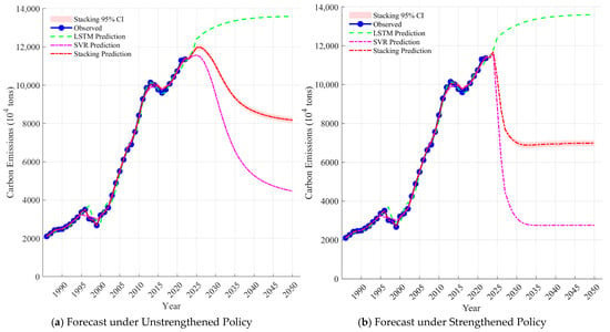
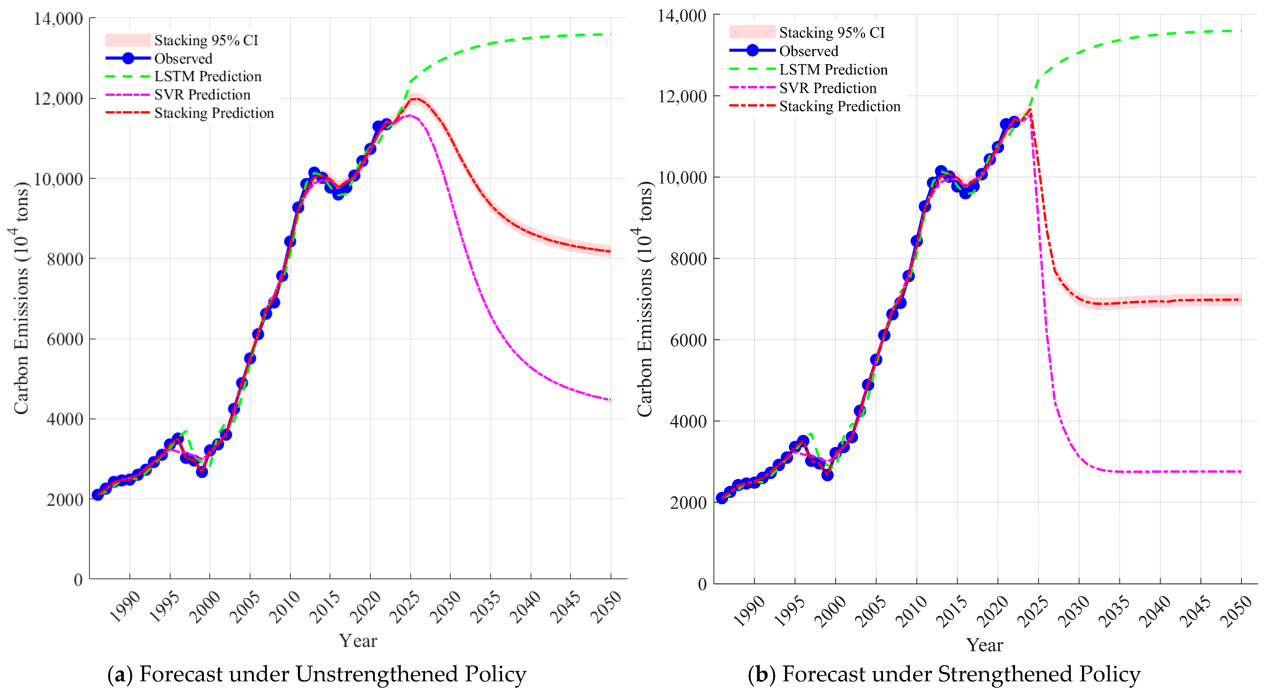
Based on the above analysis, the predictions of LSTM and SVR can be considered complementary in terms of information content, making them suitable for further ensemble modeling. Accordingly, this study employs linear regression as the meta-learner to construct a Stacking ensemble model, integrating the predictive strengths of both base models. In this framework, the period from 1960 to 2022 is used as the historical sample, while data from 2023 onward are treated as future predictions, primarily because reliable data for the explanatory variables are currently available only up to 2022. The combined prediction results are shown in Figure 3.

Figure 3. Prediction Results of Different Models.

For the prediction of the two hypothetical policy variables, this study distinguishes between Unstrengthened Policy and Strengthened Policy scenarios. In the Strengthened Policy case, 2025 is introduced as an additional future breakpoint, whereas the Unstrengthened Policy scenario retains the original three breakpoints. The combined prediction results are shown in Figure 3. Figure 3 shows that under both policy scenarios, the LSTM model generally predicts higher values, reflecting its sensitivity to temporal trends, while the SVR model exhibits an initial rise followed by a decline, capturing the influence of various constraints. The Stacking model lies between the two, retaining short-term fluctuations while simultaneously reflecting both the upward trend in the time series and the mitigating effect of policy interventions.

The model forecasts indicate that under the Unstrengthened Policy scenario, China’s carbon emissions are projected to peak around 2024 at 11,673 Mt CO₂, with a small relative error compared to the observed value of 12,603 Mt CO₂, and decline to 6983 Mt CO₂ by 2050, broadly aligning with the long-term trajectory described in the Carbon Neutrality Plan. Under the Strengthened Policy scenario, emissions are projected to peak around 2026 at 11,983 Mt CO₂, declining to 8175 Mt CO₂ by 2050, also consistent with the long-term plan. The comparison between these scenarios demonstrates that policy interventions have a significant impact on both the emission peak level and timing. These results not only confirm the robustness of the model but also highlight its utility in policy evaluation and low-carbon transition analysis, providing empirical support for China’s dual-carbon strategy and future energy planning.

5. Conclusions and Future Works

In summary, despite progress in carbon emission forecasting, key limitations persist. Time series models struggle with nonlinearity and stability; regression models, though partially interpretable, often ignore policy variables and interaction effects; AI methods achieve accuracy but have limited interpretability; and ensemble models are mostly simple integrations without deep fusion. Overall, statistical models are transparent yet weak in handling shocks, while machine learning and system models provide higher accuracy at the cost of complexity and opacity. These shortcomings constrain the ability of existing models to support long-term sustainable development, which requires both robust forecasting under uncertainty and clear policy-relevant insights. Thus, balancing predictive accuracy and interpretability, albeit less emphasized, through policy integration and advanced multi-model optimization remains a critical challenge.

To address these limitations, this study develops a forecasting framework for China’s carbon emissions by integrating time series and multivariate regression modeling. LSTM captures temporal features through multi-step prediction with BO, while SVR models nonlinear relationships among demographic, economic, energy, and policy variables, with dummy variables enhancing the model’s response to policy shocks. By explicitly embedding policy signals into the modeling process, the proposed framework links emission dynamics with sustainability-oriented governance interventions. A Stacking ensemble then integrates both models, using time series cross-validation and a linear regression meta-learner to ensure robustness and achieve accurate forecasts of carbon emission trends, while not heavily relying on interpretability. This integrated design supports sustainable development by enabling evidence-based evaluation of low-carbon transition pathways.

To validate the methodology, three experiments were conducted. First, multi-step forecasts outperformed single-step in capturing dynamic emission trends. Second, regression analysis showed that dummy variables markedly improved the model’s response to policy shocks, with trend dummies performing best. These results highlight the importance of incorporating policy-related information for assessing the sustainability impacts of emission reduction measures. Third, the Stacking ensemble surpassed standalone LSTM and SVR in predictive accuracy. Using 1980–2022 data, the model forecasted that China’s carbon emissions will peak around 2024 and decline to about 7032 Mt CO₂ by 2050. This projected pathway provides quantitative support for evaluating the long-term feasibility of China’s sustainable development and decarbonization strategies.

In conclusion, the proposed LSTM-SVR Stacking ensemble addresses key limitations of existing studies—single-model dependence, limited accuracy, and omission of policy variables—by improving forecasting precision and robustness, while relying less on interpretability. The framework provides a reliable tool for predicting carbon emission trends and supporting policy decisions on carbon peaking and neutrality. By enhancing the capacity to anticipate emission trajectories under different policy contexts, this study contributes to informed decision-making that balances economic growth, environmental protection, and social welfare. Future work should incorporate multi-source data, adopt advanced fusion strategies, and develop dynamic updating mechanisms to enhance long-term adaptability and policy relevance. Such extensions would further strengthen the model’s role in supporting sustainable development planning and climate governance.

References

- Alam, G.M.I.; Arfin Tanim, S.; Sarker, S.K.; Watanobe, Y.; Islam, R.; Mridha, M.; Nur, K. Deep learning model based prediction of vehicle CO2 emissions with eXplainable AI integration for sustainable environment. Sci. Rep. 2025, 15, 3655. [Google Scholar] [CrossRef] [Scilit]
- Wang, C.; Zhao, Y.; Yan, H.; Jiang, X.; Kang, Q.; Zhou, J. Prediction of electricity carbon emission peak in intelligent buildings with discrete second-order differential and time-sharing carbon measurement. Sustain. Energy Res. 2025, 12, 20. [Google Scholar] [CrossRef] [Scilit]
- Liu, J.-B.; Yuan, X.-Y.; Lee, C.-C. Prediction of carbon emissions in China’s construction industry using an improved grey prediction model. Sci. Total Environ. 2024, 938, 173351. [Google Scholar] [CrossRef] [Scilit]
- Hou, Y.; Liu, S. Predictive modeling and validation of carbon emissions from China’s Coastal construction industry: A BO-XGBoost ensemble approach. Sustainability 2024, 16, 4215. [Google Scholar] [CrossRef] [Scilit]
- Wang, C.; Li, M.; Yan, J. Forecasting carbon dioxide emissions: Application of a novel two-stage procedure based on machine learning models. J. Water Clim. Change 2023, 14, 477–493. [Google Scholar] [CrossRef] [Scilit]
- Chen, L.; Pan, Y.; Zhang, D. Prediction of carbon emissions level in China’s logistics industry based on the PSO-SVR model. Mathematics 2024, 12, 1980. [Google Scholar] [CrossRef] [Scilit]
- Zhong, X.; Li, X.; Li, Y. Urban expansion and carbon emission logistic curve hypothesis and its verification: A case study of Jiangsu Province. Land 2022, 11, 1066. [Google Scholar] [CrossRef] [Scilit]
- Rao, C.; Huang, Q.; Chen, L.; Goh, M.; Hu, Z. Forecasting the carbon emissions in Hubei Province under the background of carbon neutrality: A novel STIRPAT extended model with ridge regression and scenario analysis. Environ. Sci. Pollut. Res. 2023, 30, 57460–57480. [Google Scholar] [CrossRef] [Scilit]
- Zhang, P.; Ma, Y.; Wang, X.; Yang, M.; Wang, W. An Interpretable Machine Learning-Based Framework for CO2 Emission Prediction and Optimization: A Case Study of a University Campus. Sustainability 2025, 17, 10432. [Google Scholar] [CrossRef] [Scilit]
- Xie, X.; Li, Y.; Zhang, H.; Chang, Z.; Zhan, Y. Pathway Simulation and Evaluation of Carbon Neutrality in the Sichuan-Chongqing Region Based on the LEAP Model. Sustainability 2025, 17, 3233. [Google Scholar] [CrossRef] [Scilit]
- Liu, J.; Zheng, B. Scenario-based Kaya identity analysis for city-level carbon dioxide emissions. PLoS ONE 2025, 20, e0329937. [Google Scholar] [CrossRef] [Scilit]
- Feng, D.; Xu, W.; Gao, X.; Yang, Y.; Feng, S.; Yang, X.; Li, H. Carbon emission prediction and the reduction pathway in industrial parks: A scenario analysis based on the integration of the LEAP model with LMDI decomposition. Energies 2023, 16, 7356. [Google Scholar] [CrossRef] [Scilit]
- Zhang, P. Enhanced short-term carbon emission forecasting via hybrid decomposition-denoising modeling. Sci. Rep. 2025, 15, 36211. [Google Scholar] [CrossRef] [Scilit] [PubMed]
- Zhang, P.; Luo, Y.; Yu, Q.; Zhou, Z. Air transportation carbon dioxide emission forecasting: An improved back propagation neural network. PLoS ONE 2025, 20, e0333226. [Google Scholar] [CrossRef] [Scilit]
- Global Carbon Atlas. Carbon Emissions. Available online: https://globalcarbonatlas.org/emissions/carbon-emissions/ (accessed on 2 February 2026).
- Li, Y. Forecasting Chinese carbon emissions based on a novel time series prediction method. Energy Sci. Eng. 2020, 8, 2274–2285. [Google Scholar] [CrossRef] [Scilit]
- Xing, Z.; Pan, Y.; Yang, Y.; Yuan, X.; Liang, Y.; Huang, Z. Transfer learning integrating similarity analysis for short-term and long-term building energy consumption prediction. Appl. Energy 2024, 365, 123276. [Google Scholar] [CrossRef] [Scilit]
- Sagheer, A.; Hamdoun, H.; Youness, H. Deep LSTM-based transfer learning approach for coherent forecasts in hierarchical time series. Sensors 2021, 21, 4379. [Google Scholar] [CrossRef] [Scilit]
- Fang, K.; Tang, Y.; Zhang, Q.; Song, J.; Wen, Q.; Sun, H.; Ji, C.; Xu, A. Will China peak its energy-related carbon emissions by 2030? Lessons from 30 Chinese provinces. Appl. Energy 2019, 255, 113852. [Google Scholar] [CrossRef] [Scilit]
- Liu, W.; Yu, C.; Cheng, S.; Xu, J.; Wu, Y. China’s carbon emissions and trading pilot, political connection, and innovation input of publicly listed private firms. Int. J. Environ. Res. Public Health 2020, 17, 6084. [Google Scholar] [CrossRef] [Scilit] [PubMed]
- Baek, Y. Estimation of a structural break point in linear regression models. J. Bus. Econ. Stat. 2024, 42, 95–108. [Google Scholar] [CrossRef] [Scilit]
- Dafflon, J.; Da Costa, P.F.; Váša, F.; Monti, R.P.; Bzdok, D.; Hellyer, P.J.; Turkheimer, F.; Smallwood, J.; Jones, E.; Leech, R. A guided multiverse study of neuroimaging analyses. Nat. Commun. 2022, 13, 3758. [Google Scholar] [CrossRef] [Scilit]
- Dey, R.; Mathur, R. Ensemble learning method using stacking with base learner, a comparison. In Proceedings of the International Conference on Data Analytics and Insights, Kolkata, India, 11–13 May 2023; pp. 159–169. [Google Scholar]
- Maarif, M.R.; Saleh, A.R.; Habibi, M.; Fitriyani, N.L.; Syafrudin, M. Energy usage forecasting model based on long short-term memory (LSTM) and eXplainable artificial intelligence (XAI). Information 2023, 14, 265. [Google Scholar] [CrossRef] [Scilit]
- Liao, Z.; Dai, S.; Kuosmanen, T. Convex support vector regression. Eur. J. Oper. Res. 2024, 313, 858–870. [Google Scholar] [CrossRef] [Scilit]
- Safi, S.K.; Alsheryani, M.; Alrashdi, M.; Suleiman, R.; Awwad, D.; Abdalla, Z.N. Optimizing linear regression models with lasso and ridge regression: A study on UAE financial behavior during COVID-19. Migr. Lett. 2023, 20, 139–153. [Google Scholar] [CrossRef] [Scilit]
- Wu, L.; Li, J.; Zhang, J.; Wang, Z.; Tong, J.; Ding, F.; Li, M.; Feng, Y.; Li, H. Prediction model for the compressive strength of rock based on stacking ensemble learning and shapley additive explanations. Bull. Eng. Geol. Environ. 2024, 83, 439. [Google Scholar] [CrossRef] [Scilit]
- Li, Z.; Li, Y.; Shao, S. Analysis of influencing factors and trend forecast of carbon emission from energy consumption in China based on expanded STIRPAT model. Energies 2019, 12, 3054. [Google Scholar] [CrossRef] [Scilit]
- Development Strategy and Regional Economic Research Department of Development Research Center of the State Council. Available online: http://www.drc.gov.cn/n/20170824/1-224-2894327.html (accessed on 10 February 2026).
- Development Strategy and Regional Economic Research Department of the National Energy Group Energy Economics Research Institute. Available online: https://epaper.ceic.com/pc/content/202509/12/content_17081.html (accessed on 14 February 2026).
- International Economics Department; Development Data Group. World Development Indicators; World Bank: Washington, DC, USA, 2024. [Google Scholar]
- Xi, J. Report to the 19th national congress of the communist party of China. In Proceedings of the 19th National Congress of the Communist Party of China, Beijing, China, 18–24 October 2017; p. 2017. [Google Scholar]
- IEA. World Energy Outlook 2022; International Energy Agency (IEA): Paris, France, 2022; Volume 17. [Google Scholar]
- Department of Economic and Social Affairs. World Population Prospects 2024: Summary of Results; Stylus Publishing, LLC: Sterling, VA, USA, 2024. [Google Scholar]
Disclaimer/Publisher’s Note: The statements, opinions and data contained in all publications are solely those of the individual author(s) and contributor(s) and not of MDPI and/or the editor(s). MDPI and/or the editor(s) disclaim responsibility for any injury to people or property resulting from any ideas, methods, instructions or products referred to in the content. |
© 2026 by the authors. Licensee MDPI, Basel, Switzerland. This article is an open access article distributed under the terms and conditions of the Creative Commons Attribution (CC BY) license.