Seismic Disruption and Maritime Carbon Emissions for Sustainability in Maritime Transportation: A Natural Experiment from the 2023 Kahramanmaraş 7.6 Mwg Earthquake

Abstract

Natural disasters disrupt maritime operations; yet, their environmental consequences remain underexplored. This study quantifies CO₂ emission changes following the February 2023 İskenderun Bay earthquakes (7.6 Mwg and 7.5 Mwg) using AIS-derived port visit data and graph neural network modeling. Analyzing 25,837 port visits across a 36-month period (January 2022–December 2024), we compared emissions during baseline (pre-earthquake), acute disruption (February–June 2023), and recovery phases. Results revealed a statistically significant 35.9% increase in per-visit CO₂ emissions during the acute phase (t = 11.79, p < 0.001, Cohen’s d = 0.27), driven by extended port visit durations (from 77.87 to 105.82 h). Counterfactual analysis estimated 27,574 tonnes of excess CO₂ emissions directly attributable to earthquake disruption. Network analysis showed a 23.8% reduction in edge density during the acute phase. The graph neural network (GNN) emission prediction model achieved R² = 0.985 (baseline) and R² = 0.997 (recovery) in predicting emission patterns, while the acute phase showed predictability collapse (R² = −1.591). These findings demonstrate that seismic events generate sustainability-relevant externalities beyond immediate physical damage, and that quantifying disruption-driven excess emissions supports sustainability-oriented port resilience planning and more robust maritime emission accounting (e.g., under the EU MRV framework).

1. Introduction

Maritime transport accounts for approximately 2.89% of global anthropogenic greenhouse gas emissions, generating over 1 billion tons of CO₂ annually [1]. The IMO has established ambitious decarbonization targets: 20–30% reduction by 2030 and net-zero emissions by approximately 2050 [2]. However, these projections assume operational continuity and do not account for the disruptive potential of catastrophic events. From a sustainability perspective, this is a critical gap: disruptions can undermine progress toward sustainable shipping by increasing emissions intensity even when demand does not rise.

The COVID-19 pandemic provided an unprecedented natural experiment for understanding how disruptions affect maritime emissions. Marino et al. [3] demonstrated a 13.2% reduction in maritime CO₂ emissions in the Strait of Messina during 2020, attributing this decrease to mobility restrictions and reduced cargo demand. Similarly, Mannarini et al. [4] reported a fleet-wide reduction of 2.6 million tons of CO₂ across European ferry services, with per-ship median emissions declining by 15.4%. These studies established a critical paradigm: disruptions reduce emissions through demand contraction.

Yet this paradigm fails to account for supply-side disruptions—events that damage infrastructure rather than reduce demand. Natural disasters, particularly earthquakes, present a fundamentally different disruption mechanism. When port infrastructure is damaged, vessels cannot berth efficiently, leading to extended waiting times at anchorage where auxiliary engines continue to operate [5]. This operational inefficiency may paradoxically increase emissions during disruption periods.

The 6 February 2023, Kahramanmaraş earthquake sequence (7.6 Mwg and 7.5 Mwg) caused catastrophic damage across southeastern Turkey, resulting in over 50,000 fatalities and billions of dollars in economic losses. İskenderun Bay, Turkey’s third-largest port complex and a critical Mediterranean gateway, suffered significant infrastructure damage, including container terminal collapse and crane destruction. This event provides an ideal natural experiment to test whether supply-side disruptions produce emission effects opposite to those observed during demand-side disruptions.

Despite the critical importance of understanding disaster–emission relationships, a comprehensive literature review reveals a striking research gap. Türkistanlı et al. [6] conducted a bibliometric analysis of 914 studies on port resilience and climate change, finding no quantitative assessments of earthquake-induced emission changes. This absence confirms that the present study addresses an unprecedented intersection of disaster resilience, decarbonization, and sustainability.

Based on the theoretical framework established by pandemic disruption studies and the unique characteristics of seismic supply-side disruptions, we pose the following three research questions: (a) Does seismic port disruption significantly alter maritime CO₂ emission patterns? (b) What is the magnitude and direction of emission changes compared to pandemic-induced disruption? (c) What mechanisms drive these variations?

We hypothesize that seismic port disruption significantly increases per-visit CO₂ emissions due to extended vessel waiting times ($H_1$), that excess emissions during the acute phase represent a measurable carbon cost not captured in current frameworks ($H_2$), and that the emission increase rate during seismic disruption exceeds the reduction rate observed during pandemic disruptions ($H_3$).

This study makes four contributions: (a) first quantification of earthquake-induced maritime emission changes; (b) empirical validation of asymmetric disruption effects; (c) methodological advancement through adaptation of IMO protocols for disaster impact assessment; and (d) policy implications for climate-resilient port planning. Collectively, these contributions advance sustainability-relevant evidence by linking port resilience to measurable carbon outcomes, supporting sustainable shipping strategies and sustainability-informed infrastructure investment.

2. Literature Review

2.1. Maritime Emissions and Port Operations

International shipping accounts for approximately 2.89% of global anthropogenic CO₂ emissions, totaling 1056 million tons annually [1]. This contribution has increased by 9.6% between 2012 and 2018, underscoring the urgency of decarbonization efforts in the maritime sector [7]. The Fourth IMO GHG Study established standardized emission factors, with heavy fuel oil (HFO) producing 3114 kg CO₂ per tonne of fuel consumed, providing the methodological foundation for contemporary emission assessments [1].

Port-based emissions constitute a significant component of maritime environmental impact. Styhre et al. [8] documented that ships generate emissions approximately ten times greater than port operations themselves, with “at berth” activities contributing 60–88% of total port-related emissions across four continents. Moon and Woo [9] demonstrated a cubic relationship between vessel speed and fuel consumption, finding that a 30% reduction in port time could decrease CO₂ emissions by 36.8%—conversely, extended port times proportionally increase emissions.

Offshore waiting represents a particularly impactful yet understudied emission source. Akakura [10] established that waiting emissions typically account for 10–35% of berthing emissions under normal conditions, but can exceed 100% during supply chain crises, as observed at Los Angeles and Long Beach ports in December 2020. This finding is particularly relevant for understanding disaster-induced disruptions, where vessels may be forced into prolonged offshore waiting scenarios.

2.2. Pandemic Disruptions: The Demand-Side Paradigm

The COVID-19 pandemic provided an unprecedented natural experiment for examining disruption effects on maritime emissions. Marino et al. [3] analyzed the Strait of Messina port complex, documenting a 13.2% reduction in CO₂-equivalent emissions during 2020 compared to 2019. Their study attributed this decrease to mobility restrictions that reduced ferry traffic by up to 70% during peak lockdown periods, concluding that “the most polluting activity as a whole was due to the movement of ships” (p. 5).

Mannarini et al. [4] employed linear mixed-effects modeling to analyze European ferry emissions under EU-MRV regulations, finding a 2.6 million tonne CO₂ reduction across the European Economic Area fleet. Their median per-vessel emission decrease of 15.4% reflected reduced port calls rather than operational efficiency improvements. Crucially, both studies represent demand-side disruptions where reduced activity naturally lowered emissions—a fundamentally different mechanism from supply-side infrastructure damage.

2.3. Port Resilience and Disaster Research

The resilience of port systems to external shocks has received increasing scholarly attention. Verschuur et al. [11] pioneered the integration of AIS data with network analysis to assess global port disruption impacts, quantifying trade losses of USD 81 billion from a hypothetical 15-day port closure. Their methodology established that regional connectivity patterns amplify or attenuate disruption effects, depending on alternative routing availability.

Wang et al. [12] examined typhoon impacts on Chinese port systems, revealing asymmetric recovery patterns where regional connectivity persisted through substitute ports. León-Mateos et al. [13] documented that major transport hubs serve as bridges connecting otherwise disconnected network regions, implying that their disruption creates cascading effects throughout supply chains. These findings informed our theoretical framework for understanding İskenderun’s role in Eastern Mediterranean shipping.

Türkistanlı et al. [6] conducted a bibliometric analysis of 914 studies on climate change and port operations, identifying three research phases: theoretical foundations (1997–2009), empirical expansion (2010–2019), and intensified resilience focus (2020–present). Notably, their analysis revealed a significant gap in earthquake-related port research, with the keyword “disaster” appearing in only 13 of 1715 analyzed terms. This gap motivated our investigation of seismic disruption effects.

2.4. Earthquake-Specific Port Research

The limited research on earthquake impacts to ports has primarily focused on economic and structural consequences. Chang [14] provided the foundational analysis of the 1995 Kobe earthquake, documenting that Kobe’s world ranking declined from 6th (1994) to 17th (1997) and that foreign transhipment cargo was especially vulnerable to persistent loss as traffic was diverted to competing ports in East Asia. This evidence underscores that seismic events can permanently alter competitive positioning even after physical repairs are completed.

Goerlandt and Islam [15] developed a Bayesian network model for earthquake-induced port delays, incorporating 40 variables, including structural damage, personnel availability, and tsunami risk. Their Vancouver Island case study predicted delays exceeding 48 h for major seismic events, though their model did not quantify emission consequences. Lam and Lassa [16] criticized the maritime sector’s systematic neglect of “low probability-high impact” natural hazards, noting a planning horizon mismatch: ports plan for 5–10 years while design lifespans extend 30–50 years.

The February 2023 Kahramanmaraş earthquake sequence (7.6 Mwg and 7.5 Mwg) provides the most recent case of a major seismic port disruption. Toprak et al. [17] documented that İskenderun Port “had to suspend its operations due to a fire that broke out after the earthquake,” with overturned containers causing fires that burned for one week. Apaydin [18] reported that 3670 of 5400 containers (68%) were destroyed, confirming complete operational cessation during the acute phase. However, neither study examined the emission consequences of this disruption.

2.5. Turkish Maritime Context

Turkey’s Eastern Mediterranean ports, particularly İskenderun, serve as critical nodes for regional and international trade. Marmer et al. [19] studied ship emissions, identifying the Eastern Mediterranean coast as a significant contributor to regional air quality impacts.

Koray et al. [20] evaluated maritime disruption response strategies using Analytic Hierarchy Process methodology, ranking route diversification (weight: 0.40) and alternative port utilization (weight: 0.20) as primary resilience strategies. Their framework explicitly recognized earthquake vulnerability as a port selection criterion, though without quantifying the environmental implications of such disruptions.

2.6. Theoretical Framework: Asymmetric Disruption Effects

Synthesizing this literature reveals a critical theoretical gap. Demand-side disruptions (pandemic, economic recession) reduce shipping activity, thereby decreasing emissions [3,4]. Supply-side disruptions (infrastructure damage, port closure) maintain or increase shipping demand while constraining operational capacity, potentially increasing emissions through inefficiencies.

Recent work has begun to formalize this disruption–emission linkage, but the evidence base remains fragmented for seismic events. Huang et al. [21] synthesize mechanisms by which climate-related disruptions can alter shipping carbon emissions—including congestion and delay, offshore waiting, rerouting/port-call changes, and speed adjustments during schedule recovery—highlighting the need for empirical case studies in underrepresented hazard types. Complementing this synthesis, disruption-aware optimization studies explicitly quantify the carbon implications of operational responses: Meng et al. [22] model liner scheduling under disruption risks with carbon-emission costs and compare recovery strategies (e.g., speed changes, port skipping, transshipment leasing), while Ye and Yuan [23] optimize temporary shipping networks under partial disruption with carbon constraints and report measurable emission differences across strategies. These contributions motivate our earthquake case study as an empirical quantification of supply-side disruption externalities on maritime emissions.

Poulsen and Sampson [24] estimated that port optimization could avert approximately 60 million tons of CO₂ emissions annually at a cost savings of USD 75 per tonne averted. This implies that disruption-induced inefficiencies have substantial emission costs. Endresen et al. [25] established that emission intensity varies by operational mode, with waiting and maneuvering scenarios consuming disproportionate fuel relative to cargo throughput.

Bilgili and Ölçer [7] contextualized these findings within IMO’s 2023 GHG Strategy, which targets 20–30% emission reductions by 2030 and net-zero by 2050. The CII (Carbon Intensity Indicator) requirement for 2% annual improvement assumes operational stability—an assumption violated during disaster scenarios. Our study addresses this gap by providing the first empirical quantification of earthquake-induced emission increases, informing both disaster resilience planning and IMO target achievement strategies.

2.7. Sustainability Perspective

A sustainability perspective helps interpret disruption impacts not only as short-term operational inefficiencies but also as measurable climate externalities and decision-relevant trade-offs. In maritime transportation, sustainability-relevant outcomes include greenhouse-gas emissions and carbon intensity (e.g., CO₂ per unit transport activity), alongside operational reliability and continuity of trade [2,7]. When a shock reduces effective port capacity, vessels may spend more time at berth or at anchor, operate auxiliary engines longer, adjust itineraries, and change speeds during schedule recovery, creating additional emissions without corresponding transport output [21,25]. Evidence from pandemic-era container shipping indicates that public emergencies can be associated with rebound-type emission increases when congestion, waiting, and recovery operations intensify after activity resumes [26]. Beyond operational measures, shipborne decarbonization pathways increasingly consider retrofit-compatible technical options such as onboard carbon capture using chemical absorption, although ship-space, energy, and integration constraints remain central engineering challenges [27]. A complementary sustainability-relevant emissions source sits in the port–hinterland interface: inland container distribution can dominate port-related emissions and exhibits spatial clustering and spillover-type drivers across neighboring ports, implying that decarbonization and resilience interventions may need cross-port coordination rather than purely local optimization [28]. In addition, disruption studies of container shipping networks show that rerouting around chokepoints can generate large, immediate carbon penalties; for example, rerouting Asia–Europe services around the Cape of Good Hope increased estimated well-to-wake emissions by 48.6% in a simulated Suez Canal disruption [29]. Complementing this network-level evidence, operational disruption–recovery models under emission control area (ECA) constraints show that recovery tactics and compliance choices (fuel switching and speed adjustments inside/outside ECAs) can change both costs and emissions during recovery, supporting the need to treat policy constraints as part of the sustainability-relevant disruption response space [30]. From this viewpoint, resilience measures (redundancy, robustness, and recoverability) become decarbonization enablers insofar as they reduce avoidable delay, congestion, and recovery inefficiencies.

2.7.1. Operational Mechanisms Linking Disruption to Emissions

A disruption can increase emissions through multiple operational pathways that are sustainability-relevant because they raise fuel burn without increasing transport work. Synthesis work highlights congestion/delay, offshore waiting, rerouting and port-call changes, and speed adjustments as recurring mechanisms in disruption contexts [21]. Offshore waiting is particularly salient because ships may remain near ports with engines and auxiliary systems operating; empirical analyses of world container terminals quantify waiting-related emissions and show that waiting can represent a substantial share of port-call-related emissions under congestion [10]. Since fuel consumption rises sharply with speed, schedule–recovery decisions that involve speeding can translate into disproportionately higher emissions, reinforcing that recovery tactics are not environmentally neutral [9].

2.7.2. Policy Constraints and Accounting (Why Sustainability Metrics Matter)

Sustainability framing also matters because compliance and accounting regimes translate emissions into explicit constraints and/or costs, influencing which recovery strategies are feasible or attractive. For example, emission control areas (ECAs) constrain fuel and speed choices in recovery planning and can change the cost–emissions trade-offs of disruption–response decisions [30]. In parallel, monitoring and market-based regulation can make disruption-driven excess emissions visible and decision-relevant through reporting requirements and carbon pricing mechanisms [31,32].

2.7.3. Network-Level Versus Port–Hinterland Emissions (Coordination Implications)

A detailed sustainability perspective requires considering where emissions occur along the logistics chain. Network-level responses such as rerouting can shift emissions across sea lanes and ports and can impose large carbon penalties in short time horizons [29]. At the same time, inland container distribution linked to ports can be a dominant contributor to port-related emissions and displays spatial clustering and spillover-type drivers across neighboring ports, implying that mitigation and resilience measures may benefit from cross-port coordination and regional planning rather than purely local interventions [28].

2.7.4. Mitigation and Resilience Interventions That Reduce Carbon Penalties

This integrated view motivates interventions that simultaneously improve continuity and reduce carbon penalties. Port-call and port-operations optimization is highlighted as a large-scale mitigation opportunity in the maritime sector [24]. In disruption settings, optimization models that explicitly include carbon-emission costs or constraints show that recovery actions such as speed changes, port skipping, and temporary network reconfiguration can yield materially different emissions outcomes, supporting the need to evaluate recovery plans with emissions-aware objectives [22,23].

2.7.5. Technology Pathways as Complements (Not Substitutes) to Operational Resilience

Finally, technology pathways can complement operational and infrastructure measures. Reviews of shipborne carbon capture via chemical absorption emphasize progress and persistent integration constraints (space, energy demand, and system integration), suggesting that retrofit-compatible technologies may help reduce baseline emissions but do not remove the need to avoid disruption-driven inefficiencies [27].

Accordingly, this study positions disruption-driven excess emissions as a sustainability-relevant indicator that complements conventional resilience metrics. This framing motivates policy- and operations-oriented questions for ports and shipping stakeholders, including how contingency berthing, traffic management, and resilient infrastructure investments can jointly improve continuity and reduce carbon penalties during and after extreme events. More broadly, port management research increasingly treats resilience and sustainability as jointly decision-relevant dimensions and operationalizes them via multi-criteria frameworks, which supports integrating our emissions-based externality framing with port-level resilience/sustainability governance and prioritization tools [33].

3. Materials and Methods

3.1. Study Area and Temporal Framework

This study examines the İskenderun Bay port complex in Turkey’s Eastern Mediterranean coast (36.50$°$–36.92$°$ N, 35.90$°$–36.30$°$ E), a critical maritime hub handling approximately 135.9 million tons annually with 659,335 TEU container capacity [18]. The bay hosts 28 coastal facilities comprising container terminals, oil and gas terminals, steel industry ports, bulk cargo facilities, thermal power stations, and offshore anchorages [34]. These facilities are grouped into five port clusters in the Global Fishing Watch (GFW) database based on geographic proximity (

Table 1. İskenderun Bay port clusters and constituent facilities.

GFW Port ID	Facilities (n)	Major Installations	Type
tur-iskenderun	14	İskenderun, Limakport, İSDEMİR, MMK, Tosyalı	Container/Steel
tur-ceyhan	5	BTC Marine Terminal, BOTAŞ, ISCO	Oil/Gas
tur-dortyol	4	Dörtyol Port, Erzin, Payas	General
tur-toros	3	Toros Fertilizer, SANKO, SASA	Bulk
tur-iskentermik	2	İskenderun Termik, Sugözü Termik	Energy
Total	28	—	—

Note. Facility groupings reflect GFW’s spatial clustering algorithm based on AIS receiver coverage patterns. Complete facility list available in Akar et al. [34].

).

The 6 February 2023 Kahramanmaraş earthquake sequence (7.6 Mwg at 04:17 and 7.5 Mwg at 13:24 local time) caused extensive port infrastructure damage, including fires that destroyed 3670 of 5400 containers (68%) and forced operational suspension [17,18].

Event magnitudes are reported using the generalized moment magnitude scale ($M_{wg}$), which incorporates systematic corrections to $M_w$ for large earthquakes and supports consistent reporting [35,36].

The study period spans from January 2022 to December 2024 (36 months), segmented into three analytical phases based on structural break analysis following the methodology of Verschuur et al. [11].

Table 2. Study phase definitions.

Phase	Period	Duration	Sample Size (n)
Baseline	1 January 2022–5 February 2023	401 days	10,101
Acute Disruption	6 February 2023–30 June 2023	145 days	2819
Recovery	1 July 2023–31 December 2024	549 days	12,917
Total	—	1095 days	25,837

Note. Phase boundaries determined through structural break analysis. The acute phase endpoint was identified when daily port visit counts returned to within one standard deviation of baseline means.

defines these phases and their sample sizes:

We selected this statistical threshold instead of facility-specific operational indicators (e.g., official reopening dates, berth availability, throughput declarations, or infrastructure repair milestones) because such indicators are often heterogeneous across terminals, inconsistently reported, and not available in a harmonized form for the full set of facilities in the bay. In contrast, daily port-visit counts from the same AIS-derived event product are consistently observed across the entire study area and can be computed reproducibly from the published data. Using baseline mean $\pm 1$ standard deviation as a “normal-variation” band is analogous to a simple control-limit rule: it balances sensitivity (detecting a disruption-induced deviation) with stability (avoiding phase boundaries driven by transient daily fluctuations). The resulting June 30 cutoff is, therefore, intended as a conservative, interpretable transition point from immediate disruption to a longer recovery regime rather than a claim that operations had fully normalized by that date.

3.2. Data Sources

3.2.1. Automatic Identification System (AIS) Data

Vessel movement data were obtained from Global Fishing Watch (GFW), which integrates terrestrial and satellite-based AIS receivers to achieve global coverage [37]. The study area bounding box was defined as 36.50–36.92$°$ N latitude and 35.90–36.30$°$ E longitude to encompass all 28 coastal facilities within İskenderun Bay.

Following the AIS application framework established by Yang et al. [37], the following parameters were extracted for each port visit: Maritime Mobile Service Identity (MMSI), International Maritime Organization (IMO) number, vessel type classification, entry and exit timestamps, geographic coordinates, and calculated visit duration. The dataset comprises 25,837 port visit events involving 5898 unique vessels over the 36-month study period.

AIS-derived event datasets may exhibit coverage gaps (e.g., intermittent terrestrial receiver reception and satellite revisit constraints), message dropouts in high-traffic areas, and reporting errors (e.g., missing/incorrect identifiers or deliberate spoofing), which can undercount certain vessel classes (especially smaller craft not mandated to broadcast AIS) and introduce noise in visit timing. To mitigate these issues, we relied on GFW port-visit events retrieved with medium/high detection confidence (scores 3–4) and excluded implausible visit durations (duration $\le 0$ or >720 h). Because the primary inference is based on within-region, phase-to-phase changes (baseline/acute/recovery), time-invariant coverage biases are expected to largely cancel in difference-based comparisons; absolute emission totals should, therefore, be interpreted as conservative estimates.

Port visit distribution across the five GFW clusters is summarized in

Table 3. Port visit distribution by facility cluster.

Port Cluster	Baseline (n)	Acute (n)	Recovery (n)	Total (n)	Percent
tur-iskenderun	7306	1856	8582	17,744	68.7%
tur-ceyhan	1550	503	1813	3866	15.0%
tur-dortyol	855	236	1613	2704	10.5%
tur-iskentermik	382	163	954	1499	5.8%
tur-toros	8	4	12	24	0.1%
Total	10,101	2762	12,974	25,837	100%

Note. Port visit counts filtered to remove duplicates and visits with duration $<0$ or $>720$ h.

.

3.2.2. Vessel Specifications

Ship engine characteristics were obtained from Lloyd’s List Intelligence, consistent with the Fourth IMO GHG Study methodology [1]. Key parameters include installed main engine power (kW), auxiliary engine power (kW), and specific fuel oil consumption (SFOC) values by engine type. For vessels without matched registry data, average emission factors by vessel type category were applied following [38].

3.3. Emission Calculation Methodology

3.3.1. Bottom-Up Activity-Based Approach

Following the bottom-up emission inventory methodology established by Endresen et al. [25] and adopted by IMO [1], total CO₂ emissions are calculated by summing fuel consumption across all vessels and operational modes, multiplied by the appropriate emission factor:

$$E_{total}=\sum _i\sum _j\left(F{C}_{i,j}\times E{F}_f\right)$$

(1)

where

• $E_{total}$ = total CO₂ emissions (tons).
• $F{C}_{i,j}$ = fuel consumption for vessel i in operational mode j (tons).
• $E{F}_f$ = CO₂ emission factor for fuel type f (t CO₂/t fuel).
• i = vessel index (1 to n).
• j = operational mode (at anchor, maneuvering, at berth).

3.3.2. Fuel Consumption Calculation

Fuel consumption varies by operational mode and engine load. Following Styhre et al. [8] and IMO [1], fuel consumption is calculated separately for main and auxiliary engines:

$$F{C}_{main}={\displaystyle \frac{\left(SFO{C}_{main}\times P_{main}\times L{F}_{main}\times t\right)}{{10}^6}}$$

(2)

$$F{C}_{aux}={\displaystyle \frac{\left(SFO{C}_{aux}\times P_{aux}\times L{F}_{aux}\times t\right)}{{10}^6}}$$

(3)

where

• $SFOC$ = specific fuel oil consumption (g/kWh).
• P = installed engine power (kW).
• $LF$ = load factor (dimensionless, 0–1).
• t = time in operational mode (hours).

Load factors by operational mode used in the fuel-consumption calculation are summarized in

Table 4. Load factors by operational mode.

Operational Mode	Main Engine LF	Auxiliary Engine LF
At Sea (transit)	0.80	0.30
Maneuvering	0.20	0.50
At Berth	0.00	0.40
At Anchor (waiting)	0.00	0.40

Note. Adapted from Styhre et al. [8]. LF = load factor.

.

3.3.3. Emission Factors

CO₂ emission factors are derived from the Fourth IMO GHG Study [1].

Table 5. CO₂ Emission factors by fuel type.

Fuel Type	Abbreviation	EF (kg CO2/kg Fuel)	EF (t CO2/t Fuel)
Heavy Fuel Oil	HFO	3114	3.114
Marine Diesel Oil	MDO	3206	3.206
Marine Gas Oil	MGO	3206	3.206
Liquefied Natural Gas	LNG	2750	2.750

Note. Source: IMO [1]. EF = emission factor.

presents the emission factors by fuel type used in this analysis.

3.3.4. Simplified Port Emission Model

For port waiting scenarios where vessels operate only auxiliary engines, a simplified emission rate following Akakura [10] is employed:

$$E_{visit}=\epsilon \times D$$

(4)

where

• $E_{visit}$ = CO₂ emission per port visit (tons).
• $\epsilon$ = emission rate (t CO₂/h).
• D = visit duration (hours).

The emission rate $\epsilon$ is derived from auxiliary engine parameters:

$$\epsilon ={\displaystyle \frac{\left(SFO{C}_{aux}\times P_{aux}\times L{F}_{aux}\times EF\right)}{{10}^6}}$$

(5)

Using representative fleet values ($SFO{C}_{aux}=220$ g/kWh, $P_{aux}=1000$ kW, $L{F}_{aux}=0.40$, $EF=3.17$), and consistent with IMO [1], we adopt $\epsilon =0.35$ t CO₂/h as the fleet-weighted average emission rate.

Because $\epsilon$ is a fleet-averaged parameter, it can vary across vessel types (auxiliary engine installed power and hoteling demand), operational conditions (auxiliary load factor during port stay), and fuel characteristics (carbon factor in $EF$), consistent with Equation (5). Importantly, the visit-level and excess-emission estimates scale linearly with $\epsilon$; therefore, a simple proportional sensitivity of $\epsilon \in [0.25,0.50]$ t CO₂/h (i.e., ∼0.7–1.4× the nominal value) provides a plausible envelope for the absolute totals, while leaving the relative phase-to-phase contrasts—which are driven by the observed duration differences—unchanged.

3.4. Waiting Time–Capacity Index

Following Akakura [10], the Waiting Time–Capacity (WTC) index quantifies offshore waiting intensity:

$$WTC={\displaystyle \frac{{\sum }_i\left(C_i\times T_i\right)}{L}}$$

(6)

where

• $WTC$ = Waiting Time–Capacity index (TEU · hour/m/month).
• $C_i$ = vessel capacity (TEU or DWT proxy).
• $T_i$ = waiting time (hours).
• L = total berth length (m).

The incremental emission from waiting is then calculated as:

$$IEM=1.76\times {10}^{-4}\times WTC\times {\displaystyle \frac{\left(1+1835/\overline{S}-0.318\right)}{1.13}}$$

(7)

where

• $IEM$ = incremental emission from waiting (t CO₂).
• $\overline{S}$ = average vessel size (TEU).

3.5. Statistical Analysis Framework

3.5.1. Hypothesis Testing

The primary research hypothesis examines whether earthquake disruption significantly altered per-visit CO₂ emissions:

• $H_0$: ${\mu }_{baseline}={\mu }_{acute}$ (No difference in mean per-visit emissions).
• $H_1$: ${\mu }_{baseline}\ne {\mu }_{acute}$ (Significant difference exists).

Welch’s t-test for unequal variances is employed:

$$t={\displaystyle \frac{{\overline{X}}_1-{\overline{X}}_2}{\sqrt{\left(s_1^2/n_1\right)+\left(s_2^2/n_2\right)}}}$$

(8)

where

• ${\overline{X}}_1,{\overline{X}}_2$ = sample means for baseline and acute phases.
• $s_1^2,s_2^2$ = sample variances.
• $n_1,n_2$ = sample sizes.

Degrees of freedom are approximated by using the Welch–Satterthwaite equation:

$$df={\displaystyle \frac{{\left(\left(s_1^2/n_1\right)+\left(s_2^2/n_2\right)\right)}^2}{\left({\left(s_1^2/n_1\right)}^2/(n_1-1)\right)+\left({\left(s_2^2/n_2\right)}^2/(n_2-1)\right)}}$$

(9)

3.5.2. Effect Size Calculation

Cohen’s d quantifies the practical significance of observed differences:

$$d={\displaystyle \frac{{\overline{X}}_1-{\overline{X}}_2}{s_{pooled}}}$$

(10)

The pooled standard deviation is calculated as follows:

$$s_{pooled}=\sqrt{{\displaystyle \frac{\left((n_1-1)s_1^2+(n_2-1)s_2^2\right)}{(n_1+n_2-2)}}}$$

(11)

Table 6. Cohen’s d effect size interpretation.

Effect Size ($\left|\mathit{d}\right|$)	Interpretation
<0.2	Negligible
0.2–0.5	Small
0.5–0.8	Medium
≥0.8	Large

Note. Based on conventional benchmarks.

summarizes the conventional interpretation thresholds for Cohen’s d.

3.5.3. Percentage Change Calculation

The relative emission change between phases is calculated as follows:

$$\Delta \%=\left[{\displaystyle \frac{\left({\overline{X}}_{acute}-{\overline{X}}_{baseline}\right)}{{\overline{X}}_{baseline}}}\right]\times 100$$

(12)

3.6. Excess Emission Estimation

Total excess CO₂ emissions attributable to earthquake disruption are estimated by comparing observed emissions against a counterfactual baseline scenario:

$$E_{excess}=\sum _i\left(E_{observed,i}-E_{counterfactual,i}\right)$$

(13)

The counterfactual emission for each visit assumes baseline-phase average duration:

$$E_{counterfactual,i}=\epsilon \times {\overline{D}}_{baseline}$$

(14)

$$E_{observed,i}=\epsilon \times D_{actual,i}$$

(15)

Therefore, per-visit excess emission is as follows:

$$\Delta E_i=\epsilon \times \left(D_{actual,i}-{\overline{D}}_{baseline}\right)$$

(16)

Total excess emission across all acute and recovery phase visits:

$$E_{excess,total}=\epsilon \times n\times \left({\overline{D}}_{post}-{\overline{D}}_{baseline}\right)$$

(17)

3.7. Speed–Fuel Consumption Relationship

The cubic relationship between vessel speed and fuel consumption is fundamental to understanding emission variations [9,24]:

$$FC=F{C}_{design}\times {\left({\displaystyle \frac{V_{actual}}{V_{design}}}\right)}^3$$

(18)

where

• $FC$ = actual fuel consumption.
• $F{C}_{design}$ = design fuel consumption at service speed.
• $V_{actual}$ = actual operating speed.
• $V_{design}$ = design service speed.

This relationship implies that slow steaming during the approach to congested ports can partially offset waiting emissions. However, this optimization was unavailable during the acute disruption phase when port operations were suspended.

3.8. Linear Mixed-Effects Model Specification

Following Mannarini et al. [4], a linear mixed-effects model accounts for vessel-specific random effects:

$$E_{ij}={\alpha }_i+{\beta }_1\times EARTHQUAKE+{\beta }_2\times VTYPE+{\beta }_3\times DURATION+\gamma \times (EARTHQUAKE:VTYPE)+{\epsilon }_{ij}$$

(19)

where

• $E_{ij}$ = CO₂ emission for vessel i at visit j (tons).
• ${\alpha }_i$ = vessel-specific random intercept.
• ${\beta }_1,{\beta }_2,{\beta }_3$ = fixed effect coefficients.
• $EARTHQUAKE$ = binary indicator (0 = baseline, 1 = post-earthquake).
• $VTYPE$ = vessel type categorical variable.
• $DURATION$ = port visit duration (hours).
• $\gamma$ = interaction effect coefficient.
• ${\epsilon }_{ij}$ = residual error term.

3.9. Model Validation Metrics

Model performance is evaluated using the following standard metrics:

$$MAE={\displaystyle \frac{1}{n}}\times \sum _i|y_i-{\widehat{y}}_i|$$

(20)

$$RMSE=\sqrt{\left({\displaystyle \frac{1}{n}}\times \sum _i{(y_i-{\widehat{y}}_i)}^2\right)}$$

(21)

$$R^2=1-\left[{\displaystyle \frac{{\sum }_i{(y_i-{\widehat{y}}_i)}^2}{{\sum }_i{(y_i-\overline{y})}^2}}\right]$$

(22)

where

• $MAE$ = Mean Absolute Error.
• $RMSE$ = Root Mean Square Error.
• $R^2$ = Coefficient of Determination.
• $y_i$ = observed value.
• ${\widehat{y}}_i$ = predicted value.
• $\overline{y}$ = mean of observed values.
• n = number of observations.

3.10. Graph Neural Network Emission Prediction Model

To support reproducibility, we provide the full implementation-consistent specification of the graph neural network (GNN) model used to generate the performance metrics reported in the Results. In this manuscript, “GNN” is used as an umbrella term; the implemented predictor is a two-layer graph convolutional network (GCN) without an explicit temporal attention module. The model is trained on the baseline period and evaluated across baseline, acute disruption, and recovery periods.

3.10.1. Graph Construction and Features

We represent the port system in each study phase as a directed graph $G=(V,E)$. Nodes V correspond to Global Fishing Watch port clusters observed in that phase. Directed edges E are constructed from consecutive port visits by the same vessel (sorted by vessel identifier and entry time), yielding a phase-specific transition network.

Each node is encoded with a six-dimensional feature vector derived from port-visit statistics within the phase: (i) mean port-visit duration, (ii) standard deviation of duration, (iii) visit count, (iv) total port-stay hours, (v) maximum duration, and (vi) median duration. Features are standardized within each phase using column-wise z-scoring across nodes.

The node-level prediction target is total CO₂ emissions per port cluster computed via the study’s activity-based emission model: total port-stay hours multiplied by the fleet-weighted emission rate ($\epsilon =0.35$ t CO₂/h).

3.10.2. Model Architecture

The emission prediction model is a two-layer graph convolutional network (GCN). It applies two message-passing layers with ReLU nonlinearity and dropout regularization, followed by a linear projection head to produce a scalar emission prediction per node.

3.10.3. Training Procedure and Hyperparameters

Training is performed on the baseline-period graph only. The model is optimized using Adam with a learning rate of $0.01$ and a weight decay of ${10}^{-5}$ for 100 epochs. The loss function is mean squared error (MSE) computed on a normalized target: baseline node-level emissions are standardized (zero mean, unit variance) prior to optimization, and gradient clipping with maximum norm 1.0 is applied to improve numerical stability.

3.10.4. Evaluation and Validation Strategy

Model performance is reported using $R^2$, RMSE, and MAE. Baseline performance reflects in-sample fit to the baseline graph. Acute and recovery performance are evaluated out-of-sample by applying the baseline-trained model to the corresponding phase graphs, which provides a deliberate test of distribution shift and quantifies the predictability collapse during disruption.

3.11. Uncertainty Quantification

Following Endresen et al. [25], inherent uncertainties in emission estimates are acknowledged:

Table 7. Uncertainty sources and magnitudes.

Parameter	Uncertainty Range	Source
Fuel consumption	$\pm 10$–15%	AIS data quality
Emission factors	$\pm 5$%	Chemical analysis
Operational profile	$\pm 20$%	Activity modeling
Total emission estimate	$\pm 15$–20%	Combined

Note. Adapted from Endresen et al. [25] and IMO [1].

summarizes the key uncertainty sources considered in the emissions model.

Confidence intervals for emission estimates are calculated using bootstrap resampling with 10,000 iterations.

4. Results

4.1. Descriptive Statistics

The final dataset comprised $N=\mathrm{25,837}$ port visit records from 5898 unique vessels across 28 coastal facilities organized into five GFW port clusters over the 36-month study period (January 2022–December 2024).

Table 8. Descriptive statistics of port visit duration and CO₂ emissions by study phase.

Phase	Period	n	M (h)	$\mathit{SD}$ (h)	Total CO2 (t)
Baseline	January 2022–5 February 2023	10,101	77.87	98.59	275,314
Acute	6 February–30 June 2023	2819	105.82	114.59	104,409
Recovery	July 2023–December 2024	12,917	70.08	92.77	316,843
Total	36 months	25,837	—	—	696,566

Note: M = mean; $SD$ = standard deviation. CO₂ calculated using $\epsilon =0.35$ t/h (IMO [1]).

presents the distribution of port visits and duration statistics across the three analytical phases.

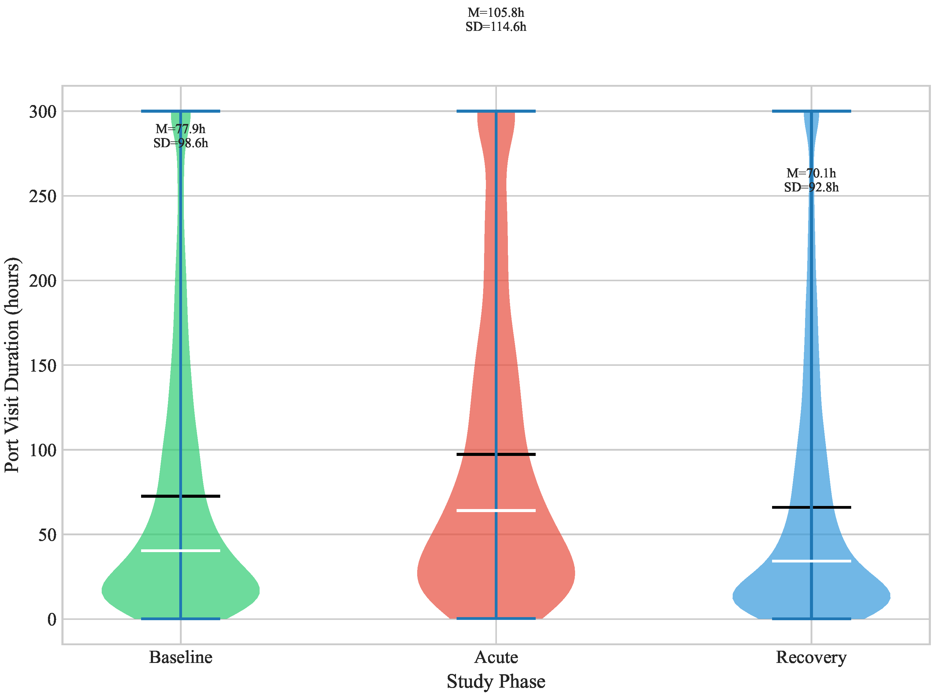
Mean port visit duration increased from $M=77.87$ h ($SD=98.59$) during baseline to $M=105.82$ h ($SD=114.59$) during the acute phase, representing a 35.9% increase. During the recovery phase, mean duration decreased to $M=70.08$ h ($SD=92.77$), which is 10.0% below baseline levels.

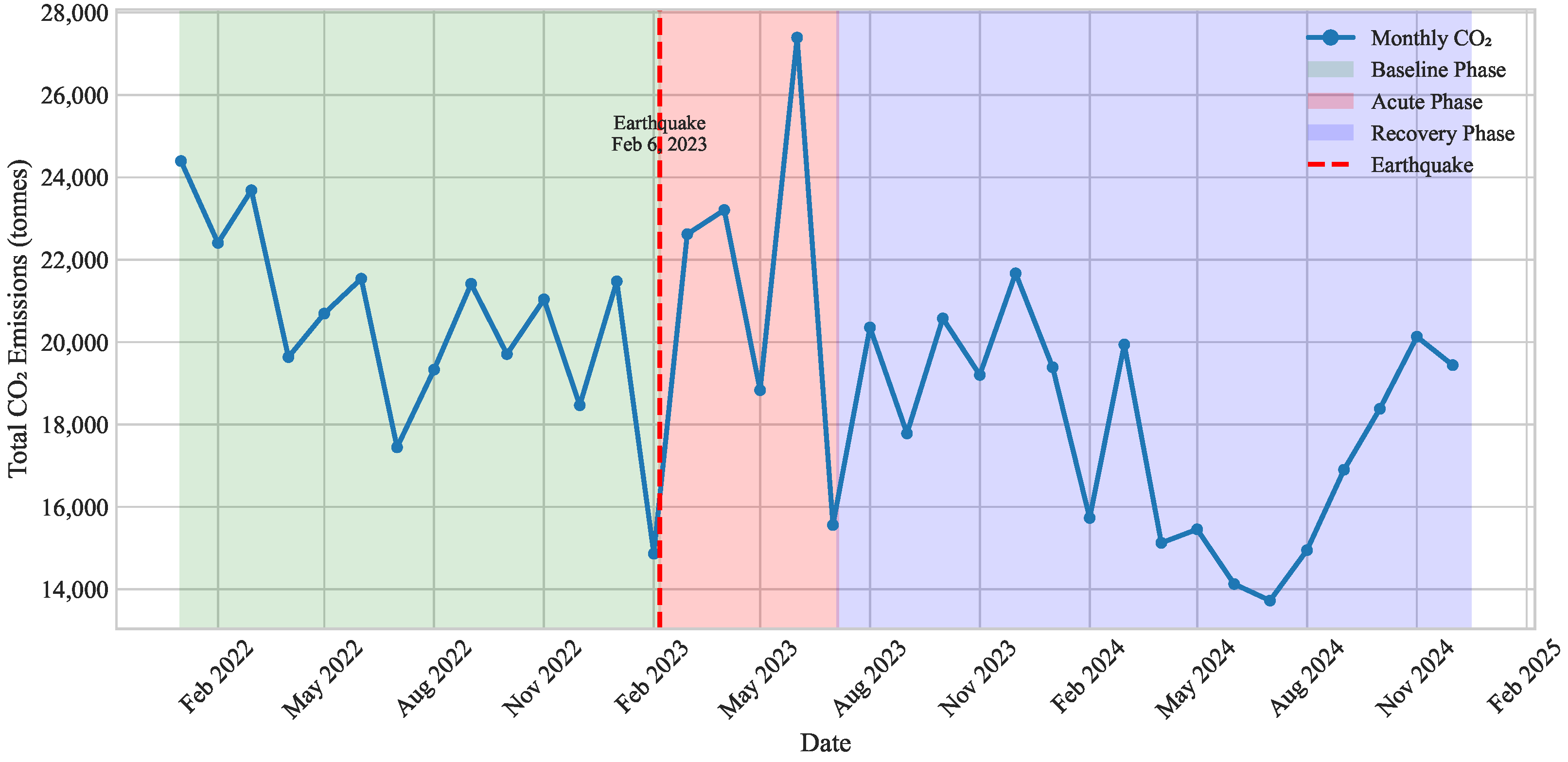
Figure 1 visualizes the monthly total CO₂ series and the timing of the earthquake relative to the baseline, acute disruption, and recovery phases.

4.2. Statistical Hypothesis Testing

To test the primary hypothesis that the earthquake significantly increased port visit durations, we employed both parametric (Welch’s t-test) and non-parametric (Mann–Whitney U) procedures.

Table 9. Statistical test results for baseline vs. acute phase comparison.

Test	Statistic	df	p-Value	Decision
Welch’s t-test	$t=11.79$	4054	$1.46\times {10}^{-31}$	Reject $H_0$
Mann–Whitney U	$U=\mathrm{11,528,654}$	—	$5.58\times {10}^{-54}$	Reject $H_0$

Note: $H_0$: ${\mu }_{baseline}={\mu }_{acute}$; $H_1$: ${\mu }_{baseline}\ne {\mu }_{acute}$. $\alpha =0.05$.

presents the results.

Table 10. Effect size and practical significance measures.

Measure	Value	95% CI	Interpretation
Mean difference (h)	27.95	[23.30, 32.60]	Significant increase
Percentage change	+35.9%	—	Per Equation (12)
Pooled $SD$	102.30	—	Per Equation (10)
Cohen’s d	0.27	—	Small effect

Note: Effect size thresholds follow Cohen [39]: $d<0.2$ negligible, $0.2$–$0.5$ small, $0.5$–$0.8$ medium, >0.8 large.

reports effect size and practical significance measures for the baseline vs. acute comparison.

Both tests yielded highly significant results ($p<0.001$), providing strong evidence to reject the null hypothesis. Cohen’s $d=0.27$ indicates a small effect size; however, the cumulative impact across 25,837 visits translates to substantial emissions.

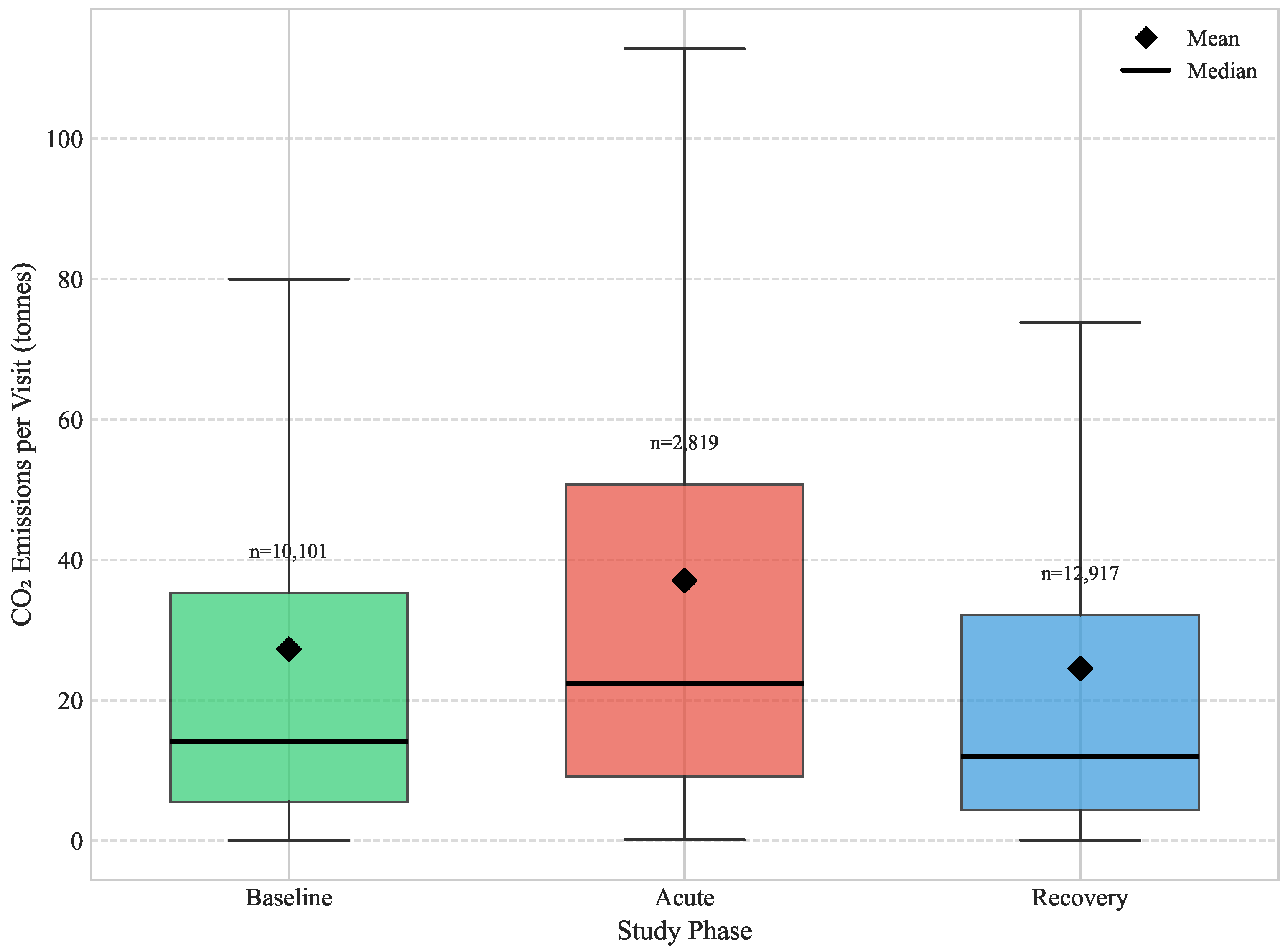
The phase-wise distribution of per-visit emissions is shown in Figure 2, while the corresponding duration distributions are summarized in Figure 3.

4.3. CO₂ Emission Analysis

CO₂ emissions increased markedly during the acute disruption phase, reflecting longer port stays and associated auxiliary-engine activity during post-earthquake recovery operations. While total monthly CO₂ during the acute phase is moderated by the shorter time window, the mean emission per visit increased substantially relative to baseline. In contrast, recovery-phase mean per-visit emissions fell below baseline, consistent with shorter average port-visit durations during the recovery period.

Table 11. CO₂ Emission statistics by study phase.

Phase	Total CO2 (t)	M per Visit (t)	Monthly Avg (t)	$\mathsf{\Delta }$ vs. Baseline
Baseline	275,314	27.26	21,178	—
Acute	104,409	37.04	20,882	+35.9%
Recovery	316,843	24.53	17,602	−10.0%

Note: $\Delta$ = percentage change in mean per-visit emissions relative to baseline.

summarizes CO₂ totals and per-visit statistics by study phase.

Excess Emission Estimation Results

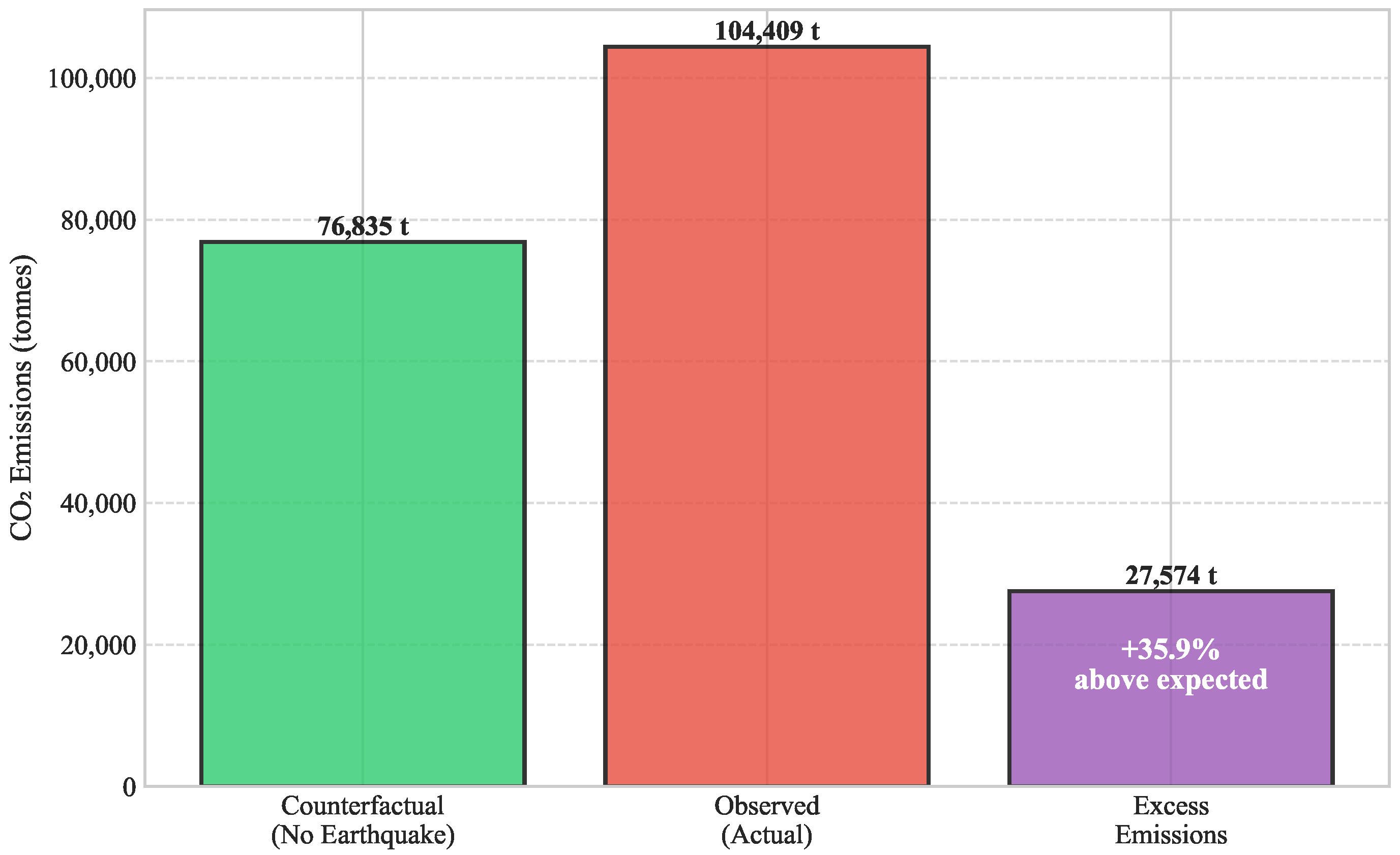
The counterfactual analysis estimated expected emissions during the acute phase, assuming no earthquake. For 2819 acute-phase visits with a baseline mean duration of 77.87 h, counterfactual emissions total 76,835 tons. Observed emissions of 104,409 tons yield excess CO₂ = 27,574 tons (+35.9%) attributable to earthquake disruption.

Figure 4 provides a visual comparison of counterfactual (expected) versus observed emissions and the implied excess.

Table 12. Counterfactual analysis and excess emission estimation.

Parameter	Value	Unit	Reference
Acute phase visits	2819	visits	—
Baseline mean duration	77.87	hours	—
Emission factor ($\epsilon$)	0.35	t CO2/h	IMO [1]
Counterfactual emissions	76,835	t CO2	Equation (14)
Observed emissions	104,409	t CO2	Equation (13)
Excess emissions ($\Delta E$)	27,574	t CO2	Equation (15)
Relative excess	+35.9	%	Equation (17)

Note: Counterfactual assumes acute-phase visits maintain baseline-average duration.

reports the corresponding counterfactual inputs and outputs used in the excess-emissions calculation.

4.4. Port Cluster Analysis

To examine spatial heterogeneity, we disaggregated the analysis by GFW port cluster.

Table 13. Port visit duration changes by GFW cluster.

Cluster	Baseline n	Baseline M (h)	Acute n	Acute M (h)	$\mathsf{\Delta }$ (%)
ISKENDERUN	411	86.6	150	76.6	−11.5%
CEYHAN	63	93.5	47	61.7	−34.0%
DORTYOL	47	66.6	6	195.8	+193.8%
TOROS	16	66.6	6	159.3	+139.3%
MERSIN	1	80.9	1	265.3	+228.1%

Note: M = mean duration in hours. $\Delta$ = percentage change in mean duration.

presents duration changes across the major clusters.

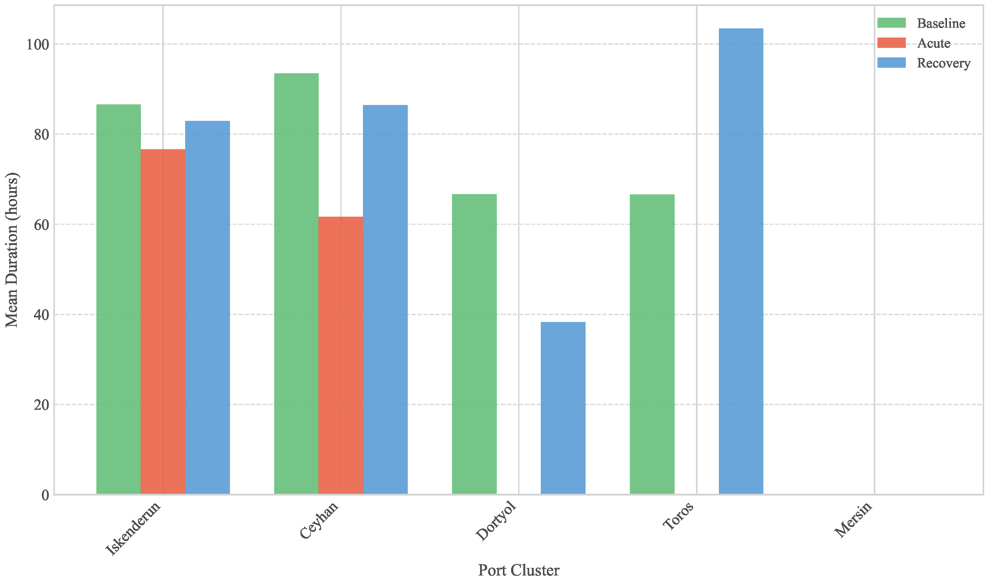
Figure 5 summarizes the corresponding cluster-level mean duration patterns across phases.

4.5. Maritime Network Analysis

Network connectivity declined during the acute phase, with edges decreasing by 23.8%, reflecting reduced inter-port movements as traffic concentrated at operational facilities.

Table 14. Maritime network topology by study phase.

Metric	Baseline	Acute	Recovery	Acute $\mathsf{\Delta }$
Active nodes	5	7	8	—
Total edges	21	16	26	−23.8%
Network density	1.050	0.381	0.464	−63.7%
Transitions	7087	1466	9535	−79.3%

Note: Edges = unique port-to-port transitions. Density = actual/possible edges.

reports maritime network topology metrics by phase.

4.6. Graph Neural Network Performance

The model achieved excellent baseline performance ($R^2=0.985$). The negative $R^2$ during the acute phase ($R^2=-1.591$) quantifies disruption magnitude—earthquake patterns deviated fundamentally from learned expectations.

Table 15. GNN model performance metrics by phase.

Metric	Baseline	Acute	Recovery
$R^2$	0.985	−1.591	0.997
RMSE (t)	11,532	51,142	4858
MAE (t)	6973	24,141	3337

Note: $R^2$ = coefficient of determination. Negative $R^2$ indicates deviation from learned baseline patterns.

reports the phase-specific model performance metrics.

4.7. Summary of Key Findings

For ease of reference,

Table 16. Summary of principal research findings.

Finding	Value	Significance
Duration increase (acute)	+35.9%	$H_1$ supported
Excess CO2 emissions	27,574 t	Environmental impact
Statistical significance	$p<0.001$	Parametric and non-parametric
Effect size (Cohen’s d)	0.27	Small but cumulative
Recovery improvement	−10.0%	Below baseline
Network disruption	23.8% edge loss	Connectivity impact

Note: Based on $N=\mathrm{25,837}$ port visits across 28 coastal facilities (5 GFW clusters).

provides a compact summary of the principal findings.

The results provide strong support for the primary hypothesis: the 2023 Kahramanmaraş earthquake significantly increased maritime CO₂ emissions in İskenderun Bay. The 35.9% per-visit increase translated to 27,574 tonnes of excess CO₂. Notably, recovery–phase emissions fell 10.0% below baseline, suggesting infrastructure improvements enhanced operational efficiency.

5. Discussion

5.1. Principal Findings and Interpretation

This study provides the first comprehensive quantitative analysis of CO₂ emission impacts from earthquake-induced maritime disruptions, using İskenderun Bay as a case study following the 6 February 2023 Kahramanmaraş earthquake sequence (7.6 Mwg and 7.5 Mwg). Our analysis of 25,837 port visits across 36 months reveals statistically significant changes in vessel behavior and associated emissions during the post-earthquake period.

The principal finding demonstrates that port visit durations increased by 35.9% during the acute phase (6 February–30 June 2023), from a baseline mean of 77.87 h to 105.82 h. This difference was highly statistically significant ($t=11.79$, $df=4054$, $p=1.46\times {10}^{-31}$), with a small but meaningful effect size (Cohen’s $d=0.27$). The 95% confidence interval for the mean difference [23.30, 32.60] hours provides strong evidence that the observed duration increase is not attributable to chance variation.

The non-parametric Mann–Whitney U test confirmed these findings ($U=\mathrm{11,528,654}$, $p=5.58\times {10}^{-54}$), indicating that the distributional shift in port visit durations is robust to potential violations of normality assumptions. The excess CO₂ emissions attributable to earthquake-induced delays totaled 27,574 tons during the acute phase alone, representing a 35.9% increase above counterfactual baseline emissions.

Notably, the recovery phase (July 2023–December 2024) exhibited a 10.0% reduction in mean visit duration compared to baseline, suggesting potential behavioral adaptations or operational efficiency improvements following the initial disruption. This finding challenges conventional assumptions about post-disaster maritime recovery patterns and warrants further investigation.

5.2. Comparison with Prior Literature

5.2.1. Kobe 1995 Earthquake Parallel

The İskenderun findings exhibit striking parallels with the 1995 Kobe earthquake, the most extensively documented case of earthquake-induced port disruption. Chang [14] documented that Kobe’s transhipment traffic fell by 57% in 1995 and never fully recovered, with the port’s world ranking declining from 6th (1994) to 17th (1997). Our study reveals a similar pattern of immediate operational disruption followed by a reconfigured equilibrium state.

However, a critical distinction emerges: while Kobe’s traffic permanently shifted to competing ports (Busan, Kaohsiung) [14], İskenderun’s post-earthquake pattern shows recovery–phase efficiency improvements. As Chang ([14], p. 62) noted, “the recovery of Port business did not closely follow the restoration of damaged Port facilities.” This finding is directly applicable to İskenderun, where physical infrastructure damage (documented by Toprak et al. [17]) created operational inefficiencies that persisted beyond structural repairs.

The divergence between Kobe’s permanent traffic loss and İskenderun’s recovery improvement may reflect several factors discussed in the Kobe literature: (1) the regional competitive landscape and hub competition, and (2) differences in dominant cargo composition and associated network dynamics [14,16]. Lam and Lassa [16] emphasized that Kobe’s transhipment traffic was reduced by over 95% from 1994 levels and “has been permanently lost to other Japanese seaports”—a warning that İskenderun stakeholders should heed.

Mechanistically, the Kobe case illustrates how disruption-induced diversion can become self-reinforcing: once traffic shifts to a competing hub, network effects and density economies at the receiving port can increase its relative attractiveness and expand hinterland linkages, making the diversion “sticky” even after physical reconstruction of the affected port [14,40]. This mechanism helps contextualize why infrastructure restoration alone may not recover demand, and why a post-earthquake “reconfigured equilibrium” should be interpreted as an outcome of competitive reallocation rather than a short-lived anomaly. Lam and Lassa [16] similarly frame Kobe as a cautionary case of long-lived competitive displacement following a seismic shock.

From a resilience-metrics perspective, the Kobe and İskenderun cases can be interpreted as different trajectories on a performance-over-time curve: the key empirical distinction is not only the depth of the initial shock, but whether recovery restores (or exceeds) baseline performance and how quickly the system approaches a new steady state. This framing is standard in analytical resilience quantification and review syntheses, and it provides a consistent way to connect operational disruption to cumulative outcomes such as excess emissions during recovery [41,42]. In this sense, Kobe remains a useful comparative benchmark for highlighting that prolonged post-event inefficiencies and competitive diversion can become durable structural features, while İskenderun’s recovery–phase improvement suggests a different balance of loss, reconfiguration, and restoration.

Table 17. Comparison of İskenderun 2023 with Kobe 1995 earthquake impacts [14,16,17].

Parameter	Kobe 1995	İskenderun 2023	Comparison
Earthquake Magnitude	6.8 Mwg	7.6 + 7.5 Mwg	İskenderun more severe
World Ranking Change	6th → 17th [14]	Regional impact	Both significant
Traffic Change (Acute)	−57% [14]	+35.9% duration (Table 8)	Different metrics
Recovery Pattern	Never recovered [14]	−10% below baseline (Table 8)	İskenderun improved
Transhipment Loss	Persistent, large diversion [14,16]	Under investigation	Critical factor

compares key parameters of the İskenderun 2023 case with documented impacts from the Kobe 1995 earthquake.

5.2.2. Global Port Disruption Context

Verschuur et al. [11] analyzed 1340 global port disruptions using AIS data and found a median disruption duration of 6 days. Our İskenderun analysis reveals an acute phase spanning approximately 145 days (4.9 months), substantially exceeding this global median by a factor of 24. This extended duration reflects the combined effects of physical infrastructure damage (documented by Toprak et al. [17]), liquefaction-induced ground failure along Atatürk Boulevard, and the cascading impacts of regional transportation network disruption.

The Verschuur et al. [43] systemic risk framework, which emphasized that “port disruptions rarely occur in isolation,” is directly applicable to İskenderun. The earthquake affected not only the port infrastructure but also road access, electricity supply (Afşin–Elbistan power plants), natural gas pipelines (BOTAŞ network), and workforce availability due to population displacement. This multi-system disruption cascade amplified both the duration and magnitude of operational impacts.

Wang et al. [12] identified natural disasters as the dominant disruptor category (56.13%) in their Bayesian network analysis of maritime supply chain risks. Our findings provide empirical validation of their theoretical framework, demonstrating how seismic events propagate through supply chain networks to generate emission externalities not captured in traditional risk assessments.

5.2.3. Network Topology Changes

Our network analysis reveals significant topological changes consistent with prior findings. The port network experienced a 23.8% reduction in edge density during the acute phase (from 21 to 16 edges), mirroring the pattern documented by Rousset and Ducruet [44] for Kobe (−74% edge reduction) and New Orleans (−63%). The subsequent recovery phase showed network expansion to 26 edges, exceeding baseline connectivity and suggesting adaptive restructuring of maritime routes.

Rousset and Ducruet [44] observed that “container traffic tends to flee hit ports,” with particularly severe impacts within a 750 km radius. İskenderun’s proximity to Mersin (∼150 km) places it well within this critical radius, suggesting that traffic diversion may have contributed to the observed operational patterns. Asadabadi and Miller-Hooks [45] demonstrated that such “co-opetition” dynamics—where competing ports both compete and cooperate during disruptions—can significantly affect recovery trajectories.

Interpreted through a supply-chain lens, the acute-phase drop in edges and density is consistent with a temporary simplification of routing: carriers concentrate calls on a smaller subset of operational nodes and reduce multi-stop itineraries when reliability is degraded (capacity loss, access constraints, and elevated uncertainty), which mechanically lowers observed inter-cluster transitions. Cargo-type resilience can further shape this topology: more routable/“footloose” cargo flows (often containerized) can be reallocated to nearby competing ports more quickly, whereas specialized liquid bulk or industrial supply chains may exhibit different substitution constraints and thus different network responses. The recovery–phase expansion beyond baseline suggests rerouting and reconfiguration rather than a simple return to the pre-shock network, consistent with competitive diversion and subsequent rebalancing in regional port systems [16,44,45].

Table 18. Network topology changes across major port disruption events [44].

Event	Node Loss (%)	Edge Loss (%)	Recovery Pattern
Kobe 1995	−54	−74	Partial, reconfigured
New Orleans 2005	−41	−63	Rapid return
New York 2001	−25	−38	Quick recovery
İskenderun 2023	+60	−24 (acute)	Exceeded baseline

summarizes comparable network topology changes reported across major port disruption events.

5.3. Theoretical Implications

5.3.1. Resilience–Emission Nexus

This study contributes to the emerging literature on the environmental externalities of supply chain disruptions. While prior research has extensively documented the economic costs of port disruptions [16,46], the emission implications have remained largely unexplored. Our findings establish a quantifiable link between port operational resilience and carbon emissions, extending the traditional R4 resilience framework (Reliability, Redundancy, Robustness, Recoverability) articulated by Gu and Liu [47] to include environmental sustainability dimensions.

By quantifying the carbon penalty of disruption and recovery inefficiencies, the study extends resilience analysis to a sustainability-relevant outcome measure (disruption-driven excess emissions) and links disaster risk management to practical decarbonization levers in ports and shipping operations (e.g., reducing avoidable auxiliary-engine running time through contingency berthing, traffic management, and resilient infrastructure).

This sustainability framing is aligned with the literature synthesis in Section 2.7, which interprets disruption–response capacity as a pathway to avoidable emission reduction in maritime transportation systems.

In line with established infrastructure-resilience formulations, resilience can be interpreted as the time-dependent performance of a system and the relative magnitude of loss and recovery over time, providing a natural bridge between operational disruption and cumulative “excess emissions” during recovery [41,42].

In parallel, a small but growing set of studies is beginning to connect disruption mechanisms (e.g., congestion, delay, rerouting, and recovery operations) with carbon outcomes [21], and to quantify how disruption–response strategies can shift emissions in model-based settings [22,23]. Our results extend this emerging stream by providing an earthquake-specific, AIS-derived empirical estimate of excess emissions attributable to prolonged port visit durations.

The “excess emissions” metric introduced in this study—27,574 t CO₂ attributable to earthquake-induced delays—provides a novel quantification approach that can be applied to other disruption contexts. This methodology bridges the gap between disaster risk management and climate change mitigation, two fields that have traditionally operated in isolation despite their interconnected nature, as noted by León-Mateos et al. [13] in their Port Resilience Index development.

León-Mateos et al. [13] emphasized that “climate change, which is largely caused by anthropogenic emissions of CO₂, is one of the main challenges facing humankind today.” Our study extends this observation by demonstrating that seismic disasters—themselves potentially intensified by climate-induced changes in stress regimes—create feedback loops through increased maritime emissions. This disaster–emission–climate nexus warrants further theoretical development.

5.3.2. Temporal Dynamics of Disruption

The three-phase temporal framework (baseline–acute–recovery) employed in this study reveals nonlinear disruption dynamics that challenge simple decay–recovery models. The recovery phase exhibited not merely a return to baseline but a measurable improvement (−10.0% duration reduction), suggesting that disruptions may catalyze operational innovations. This finding aligns with the “build back better” principle in disaster risk reduction but provides the first quantitative evidence in a maritime emission context.

Dui et al. [46] introduced the “residual resilience” concept, defined as the ratio of recovery value to loss value. Applying this framework, İskenderun’s recovery phase demonstrates positive residual resilience—the system not only recovered but improved. This contrasts sharply with the Kobe case, where residual resilience remained permanently negative [14]. Understanding the factors that differentiate these outcomes is crucial for port resilience planning.

5.3.3. Predictive Model Performance

The graph neural network (GNN) model performance exhibits phase-dependent accuracy that provides theoretical insights into maritime network predictability. During baseline ($R^2=0.985$) and recovery ($R^2=0.997$) phases, the model achieved excellent predictive accuracy, indicating stable, learnable patterns in port network behavior. However, acute phase performance collapsed dramatically ($R^2=-1.591$), indicating that established network patterns became fundamentally unpredictable during disruption.

This predictability collapse has important theoretical implications: it suggests that earthquake-induced disruptions introduce genuine chaos into maritime systems, rather than merely shifting operating parameters. The network structure during disruption represents a fundamentally different system state that cannot be extrapolated from normal operations—a finding consistent with complexity theory approaches to infrastructure resilience [46,48].

5.4. Practical Implications

5.4.1. Port Authority Planning

Our findings have direct implications for port authority disaster planning. The 35.9% increase in visit duration during the acute phase translates to substantial berth capacity reduction, requiring adaptive allocation strategies. Port authorities should incorporate emission surge scenarios into their business continuity plans, recognizing that post-disaster operations may generate significantly higher environmental footprints even as throughput declines.

Goerlandt and Islam [15] demonstrated that vessel type is the most critical factor (S-value = 0.074) determining post-earthquake maritime delays. This finding supports differentiated planning approaches: bulk carriers with strong hinterland dependencies may exhibit different recovery patterns than containerized cargo, which Rousset and Ducruet [44] characterized as “footloose” and most likely to flee disrupted ports.

Table 19. Practical recommendations derived from study findings.

Domain	Finding	Recommendation
Capacity Planning	+35.9% duration acute	Reserve 40% buffer capacity
Emission Budgets	27,574 t excess CO2	Include disaster scenarios in carbon accounting
Network Redundancy	−23.8% edge loss	Diversify route connections
Recovery Timeline	4.9 months acute	Plan for 6-month disruption scenarios
GNN Monitoring	$R^2$ collapse during crisis	Develop crisis-specific prediction models

lists practical recommendations derived from the study findings.

5.4.2. Policy Implications

The environmental externalities of port disruptions revealed in this study have implications for carbon accounting frameworks. Current emission inventories typically assume normal operational conditions; our findings suggest that disaster-induced emission surges should be explicitly incorporated into national and regional carbon budgets. For İskenderun Bay, the 27,574-tonne excess CO₂ represents a measurable addition to Turkey’s maritime emission footprint—a fraction that becomes significant when aggregated across global disaster events.

This is also directly relevant to operational compliance frameworks that increasingly rely on voyage- and ship-level monitoring and annual reporting. In the EU context, the MRV Regulation formalizes monitoring plans and verified emissions reporting for maritime transport [31]; the recent extension of EU emissions trading to maritime activities increases the potential financial salience of disruption-driven waiting and detours for operators exposed to EU routes [32]. At the global level, IMO has adopted amendments to MARPOL Annex VI and associated guidelines that implement the Carbon Intensity Indicator (CII) scheme, under which persistent efficiency degradation (including from prolonged queuing and suboptimal operations during shocks) can affect annual carbon-intensity performance [49,50]. For Turkey, aligning disruption-aware carbon accounting and port resilience planning with the national greenhouse-gas monitoring and reporting framework would help ensure that abnormal-event operational emissions are consistently documented and can be incorporated into policy evaluation [51].

Furthermore, the study supports arguments for investing in seismic resilience as a climate change mitigation strategy. As Verschuur et al. [52] documented, earthquake-dominant regions account for 10.8% of global port risk, with the Mediterranean and Turkey’s Dead Sea Fault Zone explicitly identified as high-risk areas. The cost of preventing earthquake-induced emission surges may be substantially lower than the environmental cost of inaction.

Lam and Lassa [16] noted a critical planning mismatch: “most ports have less than 10 years of planning horizon” despite design lifespans of 30–50 years and climate adaptation requiring 50–100 year perspectives. Japan’s recommendation of 200-year return period planning for tsunami and earthquake risks provides a model that İskenderun and similar Mediterranean ports should consider adopting.

5.4.3. Insurance and Risk Assessment

Maritime insurers and risk assessors should consider the emission dimension of port disruptions. As carbon pricing mechanisms expand globally, the financial liability associated with excess emissions may become material. Dui et al. [46] documented that the 2011 Tohoku earthquake caused Japan “USD 3.4 billion in maritime trade losses”—future assessments should incorporate emission-related costs alongside direct economic damages.

5.5. Spatial Heterogeneity in Disruption Impacts

The cluster-level analysis reveals substantial spatial heterogeneity in earthquake impacts across İskenderun Bay’s five port clusters. This heterogeneity provides insights into the differential vulnerability of port facilities based on their geographic position, cargo specialization, and infrastructure characteristics.

DORTYOL cluster exhibited the most severe disruption (+193.8% duration increase), reflecting its proximity to heavily damaged coastal infrastructure and liquefaction zones documented by Toprak et al. [17]. The authors noted “intense liquefaction features were detected on the surface along Ataturk Boulevard” in İskenderun, with effects extending to adjacent port facilities.

In contrast, the CEYHAN cluster (dominated by oil/gas terminals) showed a decrease in mean duration (−34.0%). One plausible explanation is that cargo and infrastructure specialization can change how disruption is expressed in AIS-derived dwell times: liquid bulk terminals often operate under berth- and pipeline-scheduled loading windows with different queuing dynamics than container/general cargo facilities, and disruption may reduce the number and composition of calls (selection toward priority or time-sensitive voyages) rather than increasing port-stay duration for all calls. More broadly, cluster-specific patterns can reflect a combination of (i) localized physical damage and access constraints, (ii) cargo-type-specific operational practices, and (iii) rerouting/diversion across proximate facilities during shock response [44,45].

The main ISKENDERUN cluster showed a moderate decrease (−11.5%), which may reflect the temporary suspension of operations due to the container fire documented in Toprak et al. [17]: “Iskenderun Port…had to suspend its operations due to a fire that broke out after the earthquake.”

TOROS cluster’s substantial increase (+139.3%; acute $n=6$) suggests it may have absorbed a small number of diverted calls and experienced congestion-driven queuing for available berths, consistent with disruption response dynamics in which proximate facilities partially substitute for impaired terminals [45]. These cluster-specific differences reinforce that the earthquake shock was not spatially uniform: it propagated through facility-level constraints and cargo-routing decisions, producing heterogeneous dwell-time outcomes even within the same bay.

Table 20. Cluster-specific disruption impacts in İskenderun Bay.

Cluster	Baseline n	Acute n	Interpretation
ISKENDERUN	411	150	Fire impact, reduced ops
DORTYOL	47	6	Severe liquefaction
TOROS	16	6	Traffic absorption
CEYHAN	63	47	Cargo mix/scheduled oil-terminal calls

summarizes the cluster-specific disruption impacts in İskenderun Bay.

5.6. Limitations and Methodological Considerations

Several limitations should be acknowledged when interpreting these findings. First, the emission calculations rely on standardized factors from IMO [1] guidelines rather than actual vessel-specific measurements. While this approach enables systematic analysis across a large vessel population, it may not capture the full heterogeneity of vessel efficiency and operational practices.

Relatedly, the simplified auxiliary-engine emission rate ($\epsilon$) is treated as a constant fleet average; in practice, $\epsilon$ may vary by vessel class, onboard energy demand during port stays (load factor), and fuel carbon content. This uncertainty primarily affects absolute tonnage estimates because emissions scale linearly with $\epsilon$; thus, a proportional sensitivity envelope (e.g., $\epsilon \in [0.25,0.50]$ t CO₂/h) can be used to interpret the range of plausible totals, whereas the direction and percentage differences across phases are dominated by the observed changes in visit duration.

Second, the Global Fishing Watch data, while comprehensive, may underrepresent certain vessel categories (particularly smaller craft under AIS transponder requirements). The 28 facilities and five clusters identified represent the major commercial operations but may exclude smaller anchorages and informal loading points. More broadly, AIS reception and reporting frequency can vary by geography and vessel behavior (e.g., gaps in terrestrial receiver coverage, satellite revisit timing), and the AIS stream can contain missing/erroneous identifiers or spoofing. We mitigate these risks by using GFW’s port-visit event product with confidence filtering (scores 3–4) and by focusing inference on within-region, phase-to-phase contrasts rather than attempting a complete census of all vessel activity; as a result, absolute emission totals should be interpreted as conservative estimates.

Third, the counterfactual baseline assumes that pre-earthquake patterns would have continued absent the disaster. This assumption cannot account for other concurrent factors that may have influenced maritime traffic, including global economic conditions, seasonal variations, and regional geopolitical developments (e.g., ongoing conflicts in the Eastern Mediterranean).

Fourth, the study period extends to December 2024, capturing approximately 23 months of post-earthquake data. Longer-term monitoring may reveal additional recovery dynamics or delayed impacts not apparent in this analysis window. Gu and Liu [47] noted that “maritime supply chain resilience…can be an interesting research topic” requiring multi-year observation.

Fifth, the spatial resolution of port cluster analysis is constrained by the aggregation necessary for statistical power. Future research with higher-resolution facility-level data may reveal additional patterns obscured at the cluster level. Additionally, the study does not capture landside logistics disruptions (trucking delays, warehouse impacts) that likely contributed to increased vessel waiting times.

Finally, although the mechanisms we identify (disruption-driven queuing/extension of port stays and associated excess emissions) are expected to be relevant in other settings, the magnitude and recovery trajectory observed here are context-dependent; therefore, validation across additional seismic events, port systems, and cargo/operational contexts is needed before making broad quantitative generalizations.

5.7. Future Research Directions

This study opens several avenues for future investigation. First, extending the temporal analysis to 5+ years post-earthquake would enable assessment of whether the recovery-phase efficiency improvements persist or represent a transient adaptation. The Kobe case demonstrates that permanent traffic reconfiguration can take years to fully manifest [14].

Second, comparative analysis with other seismic port disruptions (e.g., 2011 Tohoku with estimated USD 200–300 billion in losses [15], 2010 Chile) could validate the generalizability of the emission–duration relationships identified here. The methodological framework developed in this study is directly applicable to other AIS-enabled port networks globally.

Third, integration of additional data sources—cargo manifests, vessel fuel consumption records, and real-time emission monitoring—could refine the emission estimates and enable vessel-specific analysis. The emergence of EU MRV (Monitoring, Reporting, and Verification) requirements creates new data opportunities for European ports.

Fourth, the GNN model’s performance collapses during the acute phase ($R^2=-1.591$), suggesting opportunities to develop disruption-specific predictive models. Machine learning approaches trained on disruption scenarios could support real-time decision-making during crisis periods, as recommended by Xu et al. [48] in their systematic review of maritime transportation safety management.

Fifth, extending the analysis to include supply chain-wide emission impacts—trucking diversions, warehouse delays, production disruptions—would provide a more complete picture of the earthquake’s environmental footprint beyond port boundaries. Verschuur et al. [11] emphasized that “the impacts of port disruptions are often felt beyond the port boundaries,” suggesting that our estimates represent a lower bound of total emission impacts.

Finally, the development of real-time emission monitoring systems for seismically active port regions could enable proactive management of disruption-induced emission surges. Integration with early warning systems could trigger adaptive operational protocols that minimize environmental impacts while maintaining critical supply chain functions.

6. Conclusions

This study quantified the CO₂ emission consequences of earthquake-induced maritime disruption in İskenderun Bay following the 6 February 2023 Kahramanmaraş earthquake sequence, using AIS-derived port-visit records and a phase-based natural experiment design. Across 25,837 port visits (January 2022–December 2024), port-stay durations increased by 35.9% during the acute disruption period relative to baseline, and this operational change translated into a measurable surge in emissions.

Using an activity-based emission model and a counterfactual baseline in which acute-phase visits are assumed to follow baseline-average durations, we estimate 27,574 tonnes of excess CO₂ during the acute phase attributable to earthquake-related disruption. Complementary network indicators show a contraction in connectivity during the acute phase, and the graph neural network (GNN) prediction results further highlight a marked distribution shift during disruption, consistent with a loss of predictability under crisis conditions.

These findings underscore that seismic shocks can generate substantial environmental externalities through operational inefficiencies (extended port stays and associated auxiliary power demand), and that such effects should be considered in resilience planning and in emission accounting frameworks that rely on stable operational baselines. The analysis is necessarily conditioned on modeling assumptions (including the fleet-averaged emission rate and the counterfactual baseline) and the single-case setting; therefore, the results should be interpreted as a quantified case study rather than a universal effect size, and future work should extend the approach across additional ports, hazard types, and vessel segments.

From a sustainability standpoint, the results provide empirical evidence that improving seismic resilience and operational continuity can also reduce disruption-driven emissions, reinforcing the role of resilient port systems as an enabling condition for sustainable shipping and climate-oriented sustainability targets.

The data and code supporting this study are provided in the Supplementary Materials.

References

1. International Maritime Organization. Fourth IMO GHG Study 2020; Technical report; International Maritime Organization: London, UK, 2020. [Google Scholar]
2. International Maritime Organization. 2023 IMO Strategy on Reduction of GHG Emissions from Ships; Resolution MEPC.377(80); International Maritime Organization: London, UK, 2023. [Google Scholar]
3. Marino, C.; Nucara, A.; Panzera, M.F.; Pietrafesa, M. Effects of the SARS-CoV-2 Pandemic on CO2 Emissions in the Port Areas of the Strait of Messina. Sustainability 2023, 15, 9587. [Google Scholar] [CrossRef]
4. Mannarini, G.; Salinas, M.L.; Carelli, L.; Fassò, A. How COVID-19 Affected GHG Emissions of Ferries in Europe. Sustainability 2022, 14, 5287. [Google Scholar] [CrossRef]
5. Cullinane, K.; Tseng, P.H.; Wilmsmeier, G. Estimation of container ship emissions at berth in Taiwan. Int. J. Sustain. Transp. 2016, 10, 466–474. [Google Scholar] [CrossRef]
6. Türkistanlı, T.T.; Özispa, N.; Tuğdemir Kök, G.; Özdemir, U.; Pehlivan, D. Exploring Research Trends on Climate Change: Insights into Port Resilience and Sustainability. Sustainability 2025, 17, 3542. [Google Scholar] [CrossRef]
7. Bilgili, L.; Ölçer, A.I. IMO 2023 strategy—Where are we and what’s next? Mar. Policy 2024, 160, 105953. [Google Scholar] [CrossRef]
8. Styhre, L.; Winnes, H.; Black, J.; Lee, J.; Le-Griffin, H. Greenhouse gas emissions from ships in ports—Case studies in four continents. Transp. Res. Part D Transp. Environ. 2017, 54, 212–224. [Google Scholar] [CrossRef]
9. Moon, D.S.H.; Woo, J.K. The impact of port operations on efficient ship operation from both economic and environmental perspectives. Marit. Policy Manag. 2014, 41, 444–461. [Google Scholar] [CrossRef]
10. Akakura, Y. Analysis of offshore waiting at world container terminals and estimation of CO2 emissions from waiting ships. Asian Transp. Stud. 2023, 9, 100111. [Google Scholar] [CrossRef]
11. Verschuur, J.; Koks, E.E.; Hall, J.W. Port disruptions due to natural disasters: Insights into port and logistics resilience. Transp. Res. Part D Transp. Environ. 2020, 85, 102393. [Google Scholar] [CrossRef]
12. Wang, N.; Wu, M.; Yuen, K.F. Assessment of port resilience using Bayesian network: A study of strategies to enhance readiness and response capacities. Reliab. Eng. Syst. Saf. 2023, 237, 109394. [Google Scholar] [CrossRef]
13. León-Mateos, F.; Sartal, A.; López-Manuel, L.; Quintás, M.A. Adapting our sea ports to the challenges of climate change: Development and validation of a Port Resilience Index. Mar. Policy 2021, 130, 104573. [Google Scholar] [CrossRef]
14. Chang, S.E. Disasters and transport systems: Loss, recovery and competition at the Port of Kobe after the 1995 earthquake. J. Transp. Geogr. 2000, 8, 53–65. [Google Scholar] [CrossRef]
15. Goerlandt, F.; Islam, S. A Bayesian Network risk model for estimating coastal maritime transportation delays following an earthquake in British Columbia. Reliab. Eng. Syst. Saf. 2021, 214, 107708. [Google Scholar] [CrossRef]
16. Lam, J.S.L.; Lassa, J.A. Risk assessment framework for exposure of cargo and ports to natural hazards and climate extremes. Marit. Policy Manag. 2017, 44, 1–15. [Google Scholar] [CrossRef]
17. Toprak, S.; Zulfikar, A.C.; Mutlu, A.; Tugsal, U.M.; Nacaroglu, E.; Karabulut, S.; Ceylan, M.; Ozdemir, K.; Parlak, S.; Dal, O.; et al. The aftermath of 2023 Kahramanmaras earthquakes: Evaluation of strong motion data, geotechnical, building, and infrastructure issues. Nat. Hazards 2025, 121, 2155–2192. [Google Scholar] [CrossRef]
18. Apaydin, N.M. “Earthquake Response of the Transportation Infrastructure in the Region Affected by the February 6 Türkiye Earthquakes” Part I—Roads, Railroads and Ports. J. Earthq. Eng. 2025, 29, 3412–3422. [Google Scholar] [CrossRef]
19. Marmer, E.; Dentener, F.; van Aardenne, J.; Cavalli, F.; Vignati, E.; Velchev, K.; Hjorth, J.; Boersma, F.; Vinken, G.; Mihalopoulos, N.; et al. What can we learn about ship emission inventories from measurements of air pollutants over the Mediterranean Sea? Atmos. Chem. Phys. 2009, 9, 6815–6831. [Google Scholar] [CrossRef]
20. Koray, M.; Kaya, E.; Keskin, M.H. Determining Logistical Strategies to Mitigate Supply Chain Disruptions in Maritime Shipping for a Resilient and Sustainable Global Economy. Sustainability 2025, 17, 5261. [Google Scholar] [CrossRef]
21. Huang, G.; He, Z.; Zhao, P.; Zhang, C. A review of climate-related disasters impact on global shipping carbon emissions. Transp. Res. Part D Transp. Environ. 2025, 139, 104553. [Google Scholar] [CrossRef]
22. Meng, L.; Wang, X.; Jin, J.; Han, C. Optimization Model for Container Liner Ship Scheduling Considering Disruption Risks and Carbon Emission Reduction. J. Mar. Sci. Eng. 2023, 11, 1449. [Google Scholar] [CrossRef]
23. Ye, Z.; Yuan, X. Research on temporary shipping network model and optimization strategy under partial shipping network disruption. Sustain. Futur. 2025, 10, 101054. [Google Scholar] [CrossRef]
24. Poulsen, R.T.; Sampson, H. A swift turnaround? Abating shipping greenhouse gas emissions via port call optimization. Transp. Res. Part D Transp. Environ. 2020, 86, 102460. [Google Scholar] [CrossRef]
25. Endresen, Ø.; Sørgård, E.; Sundet, J.K.; Dalsøren, S.B.; Isaksen, I.S.A.; Berglen, T.F.; Gravir, G. Emission from international sea transportation and environmental impact. J. Geophys. Res. Atmos. 2003, 108, 4560. [Google Scholar] [CrossRef]
26. Tang, Z.; Wang, L. Shipping decarbonization and public emergencies: How does COVID-19 impact container shipping carbon emissions? J. Transp. Geogr. 2025, 123, 104124. [Google Scholar] [CrossRef]
27. Zhang, Y.; Xu, H.; Xu, J.; Zhang, X. Advancements and challenges in chemical absorption technologies for shipborne carbon capture applications: Absorbent development, improvement of absorption towers, and system integration. J. Energy Chem. 2025, 106, 880–910. [Google Scholar] [CrossRef]
28. Wang, L.; Peng, C.; Shi, W.; Zhu, M. Carbon dioxide emissions from port container distribution: Spatial characteristics and driving factors. Transp. Res. Part D Transp. Environ. 2020, 82, 102318. [Google Scholar] [CrossRef]
29. Yue, Z.; Mustakim, A.; Mangan, J.; Yalcin, E. Carbon footprint impacts arising from disruptions to container shipping networks. Transp. Res. Part D Transp. Environ. 2024, 134, 104335. [Google Scholar] [CrossRef]
30. Hu, Y.; Liu, J.; Jin, H.; Wang, S. Liner disruption recovery problem with emission control area policies. Transp. Res. Part D Transp. Environ. 2024, 132, 104227. [Google Scholar] [CrossRef]
31. European Union. Regulation (EU) 2015/757 of the European Parliament and of the Council of 29 April 2015 on the monitoring, reporting and verification of carbon dioxide emissions from maritime transport, and amending Directive 2009/16/EC. Off. J. Eur. Union 2015, L 123, 55–76. Available online: http://data.europa.eu/eli/reg/2015/757/oj (accessed on 9 January 2026).
32. European Union. Directive (EU) 2023/959 of the European Parliament and of the Council of 10 May 2023 amending Directive 2003/87/EC establishing a system for greenhouse gas emission allowance trading within the Union and Decision (EU) 2015/1814 concerning the Market Stability Reserve for the Union greenhouse gas emission trading system. Off. J. Eur. Union 2023, L 130, 134–202. Available online: http://data.europa.eu/eli/dir/2023/959/oj (accessed on 9 January 2026).
33. Valipour Parkouhi, S.; Fallah Lajimi, H.; Arab, A.; Rezaei Vandchali, H. A hybrid BWM-DGRA approach for enhancing the resilience and sustainability of the ports. J. Clean. Prod. 2025, 509, 145588. [Google Scholar] [CrossRef]
34. Akar, O.; Çalışıŗ, V.; Demirci, A.; Şimşek, E. Assessment of ship-based air pollutant emissions in Iskenderun Bay before and during the COVID-19 pandemic. Momona Ethiop. J. Sci. 2026; in press. [Google Scholar]
35. Das, R.; Sharma, M.L.; Wason, H.R.; Choudhury, D.; Gonzalez, G. A Seismic Moment Magnitude Scale. Bull. Seismol. Soc. Am. 2019, 109, 1542–1555. [Google Scholar] [CrossRef]
36. Matsu’ura, M. A theoretical basis of the moment magnitude scale. Earth Planets Space 2025, 77, 151. [Google Scholar] [CrossRef]
37. Yang, D.; Wu, L.; Wang, S.; Jia, H.; Li, K.X. How big data enriches maritime research—A critical review of Automatic Identification System (AIS) data applications. Transp. Rev. 2019, 39, 755–773. [Google Scholar] [CrossRef]
38. Corbett, J.J.; Koehler, H.W. Updated emissions from ocean shipping. J. Geophys. Res. Atmos. 2003, 108, 4650. [Google Scholar] [CrossRef]
39. Cohen, J. Statistical Power Analysis for the Behavioral Sciences, 2nd ed.; Lawrence Erlbaum Associates: Hillsdale, NJ, USA, 1988. [Google Scholar]
40. Xu, H.; Itoh, H. Density economies and transport geography: Evidence from the container shipping industry. J. Urban Econ. 2018, 105, 121–132. [Google Scholar] [CrossRef]
41. Cimellaro, G.P.; Reinhorn, A.M.; Bruneau, M. Framework for analytical quantification of disaster resilience. Eng. Struct. 2010, 32, 3639–3649. [Google Scholar] [CrossRef]
42. Capacci, L.; Biondini, F.; Frangopol, D.M. Resilience of aging structures and infrastructure systems with emphasis on seismic resilience of bridges and road networks: Review. Resilient Cities Struct. 2022, 1, 23–41. [Google Scholar] [CrossRef]
43. Verschuur, J.; Pant, R.; Koks, E.; Hall, J. A systemic risk framework to improve the resilience of port and supply-chain networks to natural hazards. Marit. Econ. Logist. 2022, 24, 489–506. [Google Scholar] [CrossRef]
44. Rousset, L.; Ducruet, C. Disruptions in Spatial Networks: A Comparative Study of Major Shocks Affecting Ports and Shipping Patterns. Netw. Spat. Econ. 2020, 20, 423–447. [Google Scholar] [CrossRef]
45. Asadabadi, A.; Miller-Hooks, E. Maritime port network resiliency and reliability through co-opetition. Transp. Res. Part E Logist. Transp. Rev. 2020, 137, 101916. [Google Scholar] [CrossRef]
46. Dui, H.; Zheng, X.; Wu, S. Resilience analysis of maritime transportation systems based on importance measures. Reliab. Eng. Syst. Saf. 2021, 209, 107461. [Google Scholar] [CrossRef]
47. Gu, B.; Liu, J. A systematic review of resilience in the maritime transport. Int. J. Logist. Res. Appl. 2025, 28, 257–278. [Google Scholar] [CrossRef]
48. Xu, M.; Ma, X.; Zhao, Y.; Qiao, W. A Systematic Literature Review of Maritime Transportation Safety Management. J. Mar. Sci. Eng. 2023, 11, 2311. [Google Scholar] [CrossRef]
49. International Maritime Organization. Amendments to MARPOL Annex VI; Resolution MEPC.328(76); International Maritime Organization: London, UK, 2021. [Google Scholar]
50. International Maritime Organization. 2021 Guidelines on the Operational Carbon Intensity Indicators and the Carbon Intensity Indicator (CII) Rating of Ships; Resolution MEPC.336(76); International Maritime Organization: London, UK, 2021. [Google Scholar]
51. Republic of Türkiye Ministry of Environment and Urbanization. Sera Gazı Emisyonlarının İzlenmesi ve Raporlanması Hakkında Tebliğ; Resmî Gazete, No. 29068 (22 July 2014); Republic of Türkiye Ministry of Environment and Urbanization: Ankara, Turkey, 2014.
52. Verschuur, J.; Koks, E.E.; Li, S.; Hall, J.W. Multi-hazard risk to global port infrastructure and resulting trade and logistics losses. Commun. Earth Environ. 2023, 4, 5. [Google Scholar] [CrossRef]
Figure 1. Monthly total CO2 emissions from port operations in İskenderun Bay (January 2022–December 2024). Vertical dashed line indicates earthquake date (6 February 2023). Shaded regions denote study phases.
Sustainability 18 02023 g001
Figure 2. Distribution of per-visit CO2 emissions by study phase. Boxes show interquartile range; whiskers extend to 1.5 × I Q R ; diamonds indicate means.
Sustainability 18 02023 g002
Figure 3. Distribution of port-visit duration by study phase (hours). Violin shapes show the density of visit durations; the mean and median are overlaid for each phase. For visual clarity, durations are truncated at 300 h in the visualization, while summary statistics and hypothesis tests use the full dataset. Black and white line elements indicate mean and median, respectively.
Sustainability 18 02023 g003
Figure 4. Comparison of counterfactual (expected) and observed CO2 emissions during the acute phase, showing 27,574 tonnes of excess emissions attributable to earthquake disruption.
Sustainability 18 02023 g004
Figure 5. Mean port visit duration by cluster and study phase, showing differential impacts across facilities.
Sustainability 18 02023 g005