


Abstract
The characterization and prediction of seasonal variations in river water quality are essential for maintaining control of aquatic ecosystems and resource management. This study aims to develop predictive models using Artificial Intelligence (AI) techniques, particularly Machine Learning (ML) algorithms, to classify seasonal patterns in three major rivers in Bangladesh: Buriganga, Shitalakhya, and Turag. This study considered 15 of the most significant water quality parameters, including pH, alkalinity, biochemical oxygen demand (BOD), chemical oxygen demand (COD), total dissolved solids (TDSs), and electrical conductivity (EC). A total of 476 samples were gathered on a monthly basis at 17 monitoring points in the three rivers, covering all months between January and December from 2021 to 2023. With K-fold cross-validation and hyperparameter optimization, three ML models, like Extreme Gradient Boosting (XGBoost), Random Forest (RF), and Decision Tree (DT), were employed for predicting seasonal variation in river water quality. The models were assessed based on accuracy, precision, recall, F1, and ROC–AUC scores. Partial Dependence Plot (PDP) analysis was applied to explore the marginal effects of key water quality features on seasonal prediction while keeping other variables constant. RF achieved the highest accuracy of 79%, and XGBoost was about 77% among the models. The achieved prediction accuracies indicate a robust capability to capture key seasonal and spatial changes in river water quality. At this performance level, the models are effective in identifying conditions associated with deteriorated water quality and potential exceedances of guideline-based thresholds established by the World Health Organization (WHO) and Bangladesh water quality standards, supporting timely assessment and management interventions. The SHAP analysis demonstrated TDS, alkalinity, and EC as the top feature drivers of seasonal differences, providing insight into the interplay between chemical composition and climate. The results of the study have the potential to accurately depict the seasonal patterns in river water quality using AI approaches.
1. Introduction
Seasonal variation indicates the periodic alteration of environmental and hydrological conditions such as temperature, rainfall, river discharge, and evapotranspiration, occurring over defined temporal cycles within a season [1]. These variations have a profound influence on the photochemical composition of river systems, thereby impacting overall water quality. The River Water Quality Index (WQI) work as a comprehensive indicator that encapsulates many physicochemical parameters, such as pH, dissolved oxygen (DO), biochemical oxygen demand (BOD), chemical oxygen demand (COD), total dissolved solids (TDS), turbidity and electrical conductivity (EC) into a single numerical value reflecting the water ecosystem’s health [2]. Consequently, the fundamental interaction between seasonal dynamics and river water quality plays a pivotal role in determining ecosystem stability, pollutant dispersion, and the sustainability of freshwater resources [3]. Acknowledging these temporal fluctuations is thus an obligation for effective water resource management, environmental policymaking, and moderation of anthropogenic impacts [4].
Globally, as well as within Bangladesh, river water quality is highly sensitive to seasonal cycles driven by climatic and hydrological factors [5]. For instance, the monsoon season induces increased surface runoff and sedimentation, leading to higher turbidity and nutrient loads. Whereas the dry season often results in reduced river flow and concentrated pollutant levels [6]. Identical dependencies have been reported worldwide where rivers in tropical, subtropical, and temperate areas exhibit distinct physicochemical variations in response to shifts in precipitation patterns, temperature regimes, and human activities [7]. Parameters such as DO, BOD, TDS, and EC display pronounced temporal variability, reflecting the influence of natural processes and anthropogenic stressors [8].
However, river water systems are increasingly threatened by seasonal fluctuations in flow and pollutant loadings, which severely alter their physicochemical composition and ecological balance [9]. In many developing regions, including Bangladesh, inadequate wastewater treatment, unregulated industrial discharge, and agricultural runoff further exacerbate the seasonal degradation of river water quality, particularly during low-flow periods [9,10]. Moreover, the absence of continuous monitoring systems and limited analytical capacity makes it difficult to evaluate the temporal changes in key parameters such as DO, BOD, and EC, resulting in ineffective water quality management practices [11]. The complexity of seasonal interactions, driven by climatic, hydrological, and anthropogenic factors, poses a serious challenge to understanding and predicting water quality dynamics using traditional statistical techniques [12]. Therefore, there is a pressing need for intelligent, data-driven systems capable of capturing nonlinear seasonal behavior and providing reliable predictions for sustainable water resource management [13].
Considering these consequences, this study aims to predict seasonal variations in river water quality by applying AI and ML techniques [14]. This study aims to classify and predict seasonal variations in river water quality using fifteen physicochemical indicators through three machine learning models: RF, DT, and XGBoost. Four seasonal prediction models were developed to capture the distinct characteristics of the pre-monsoon, monsoon, post-monsoon, and winter. Model performance was assessed using standard evaluation metrics, including accuracy, recall, and F1-score, leading to the selection of three optimized models for subsequent validation and application [15]. The confusion matrix was employed to ensure stable and consistent classification across seasonal categories, while the ROC–AUC analysis was applied to evaluate the discriminative ability and robustness of the models in distinguishing between different seasonal classes. In addition, data-driven analytical techniques were integrated to explore nonlinear dependencies among the physicochemical parameters and to identify dominant features influencing seasonal transitions using SHAP analysis. The results indicated that total TDS, alkalinity, and EC were the most influential parameters governing seasonal variation, emphasizing the complex relationship between chemical composition and climatic fluctuations. Subsequently, the PDP analysis was conducted based on the most influential features to interpret their marginal effects on seasonal classification. The outcomes of this research highlight the potential of AI-driven predictive modeling as an effective framework for sustainable monitoring and management of river water quality. By enabling early detection of water quality deterioration and improving predictive reliability, the proposed data-driven approach can assist policymakers, environmental engineers, and researchers in formulating adaptive and evidence-based strategies for safeguarding aquatic ecosystems against the impacts of seasonal and climatic considerations. The paper is structured as follows: Section 2 presents the materials and methods, including background studies, data collection and cleaning, model development, and feature selection. Section 3 presents the study’s results, while Section 4 discusses comparative studies, including limitations and future scope. Finally, Section 5 provides the concluding remarks.
2. Materials and Methods
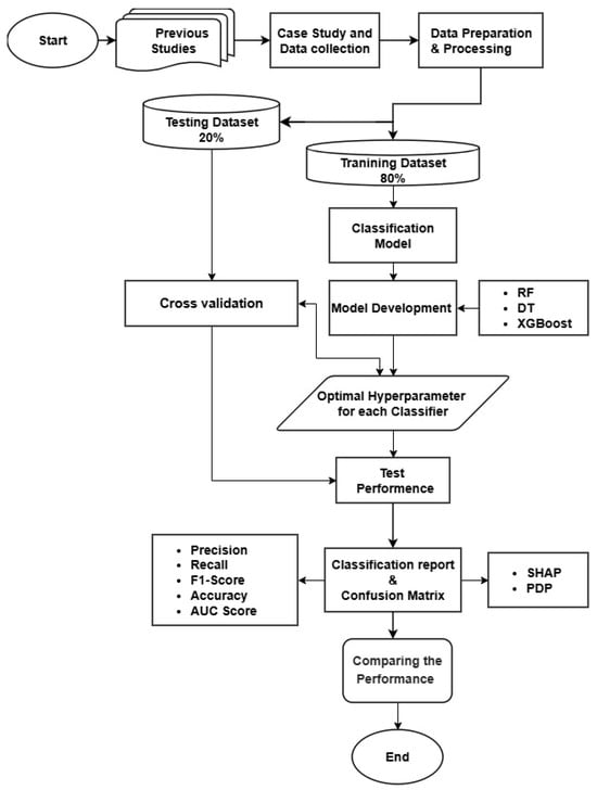
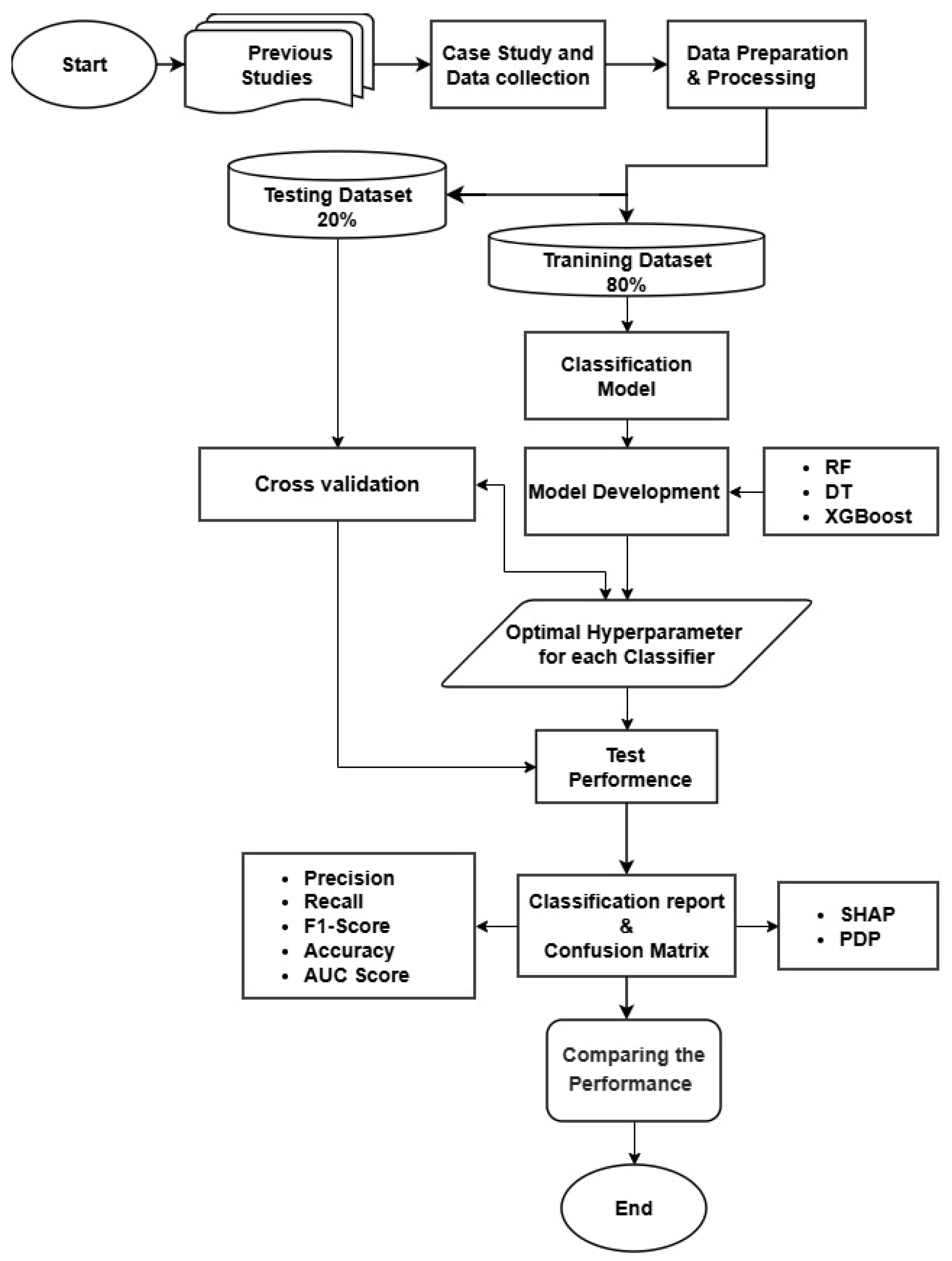
The methodological framework, illustrated in Figure 1, outlines a systematic workflow beginning with previous studies and encompassing data collection and preparation, model development, and performance evaluation. Seasonal variation classification was processed and divided into training and testing subsets. Three ML models: RF, DT, and XGBoost—were optimized through hyperparameter tuning and cross-validation. The model’s robustness was evaluated using accuracy, the F1 score, the confusion matrix, and the AUC score, while SHAP analysis was applied to rank features and improve interpretability. Additionally, PDP applied to explore the marginal effects of key water quality features on seasonal prediction.
Figure 1.
Flow chart of research method.
2.1. Background from Previous Studies
Understanding and predicting the seasonal variation in river water quality is essential for keeping the aquatic ecosystem healthy and for the sustainable management of our water resources [5]. River water quality changes naturally from season to season due to variations in rainfall, temperature, and river flow [12]. During the wet season, heavy rainfall and surface runoff often carry sediments, nutrients, and pollutants from surrounding land into rivers, which can temporarily reduce water quality [16]. In contrast, the dry season is usually marked by lower river flow and higher water temperatures, allowing pollutants to become more concentrated and dissolved oxygen levels to decrease. These seasonal changes strongly influence river health and aquatic life [17]. Therefore, understanding seasonal water quality patterns helps policymakers and water managers design effective and targeted river water quality monitoring programs.
Although environmental monitoring has been extensively studied over the years, the recent integration of Artificial Intelligence (AI) and Machine Learning (ML) has introduced a new direction in this field, effectively addressing many of the limitations associated with traditional approaches. Previously, most water quality forecasting models relied on statistical and numerical approaches, similar to the air quality studies conducted decades earlier [18]. But these old methods, which mostly depend on deterministic or simple physical assumptions, are not very effective in complex river systems. One of the main problems is that they rely on incomplete or missing input data and oversimplified assumptions, which often cause big forecasting errors in real-world conditions [19]. Furthermore, traditional monitoring systems are slow, costly, and unable to provide the high-frequency data required for rapid and effective water management. For example, Land Use Regression (LUR) models mainly focus on spatial patterns but ignore temporal changes, so they are not very suitable for predicting dynamic environmental quality [20].
Machine learning has become a strong alternative because of its ability to give better and more reliable predictions [21]. Researchers have already used ML models successfully in many environmental problems. For example, in air quality prediction, the STA-LSTM model was used to improve accuracy across different locations and time intervals [22]. Similarly, hybrid approaches that combine simulation-based and data-driven methods, as in energy use studies or climate-resilient occupant comfort assessments, show that integrated ML models can perform effectively in environmental applications such as water quality prediction [23,24,25,26]. In the case of water quality, some algorithms like Random Forest (RF), Multilayer Perceptron (MLP), and Adaptive Neuro Fuzzy Inference System (ANFIS) are found to be really effective for real-time monitoring, and they often give better results compared to the old traditional models [27]. These results show that ML-based models can capture the complex and nonlinear relations among water quality parameters better than physics-based models alone. Even though many studies have used ML for water quality prediction, there are still limited works that directly focus on predicting or classifying seasonal variations in water quality [28]. Seasonal changes bring huge differences due to rainfall, temperature, and flow rate, which make it very difficult for simple models to maintain accuracy [29]. Some studies have already proved that ML could predict parameters like Dissolved Oxygen (DO) and Biochemical Oxygen Demand (BOD) quite successfully [30,31,32].
Despite notable progress in ML applications for river water quality, several research gaps remain. A complete framework that classifies seasonal patterns across multiple rivers using diverse physicochemical parameters is still missing. Another key limitation concerns model interpretability; understanding why a model generates certain outputs is essential for transparency and trust. For instance, simply predicting whether water quality will deteriorate or improve offers limited value; it is more informative to identify how influential parameters such as TDS and alkalinity vary and drive water quality changes under different seasonal conditions. However, many previous studies overlooked this type of feature-based explanation, hindering the practical applicability of model results in environmental management. For example, Lokman et al. note evaluation of model interpretability is rarely addressed in water quality forecasting [33]. Amini et al. demonstrated TDS prediction in the Karkheh River using machine learning, with signal-driven features improving RMSE by 30% and enabling scalable real-time water quality monitoring [34]. Also, Xu et al. decoded river pollution trends and their landscape determinants in an ecologically fragile karst basin using a ML model, with SHAP analysis indicating that pollutant levels are driven by anthropogenic sources, fragile soils, and pollutant transport mechanisms [35]. Melesse et al. predicted river water salinity using hybrid ML models, showing that hybrid algorithms generally enhance predictive performance and better capture maximum salinity values, which is crucial for water resource management [36]. Furthermore, existing research rarely accounts for spatial heterogeneity across monitoring locations, yet differences between rivers or sites (e.g., urban versus rural, upstream vs. downstream) can significantly affect the generalizability and robustness of predictive models. Also, comparative evaluations among different AI/ensemble classifiers are often missing, leaving uncertainty regarding which model architecture is most suitable for seasonal water quality classification tasks. For example, a recent Bangladesh study compared many models for WQI prediction in urban rivers but did not delve into seasonal-pattern classification or parameter-based explanations [37].
To address these gaps, this study develops an AI-based framework for classifying seasonal river water quality patterns in Bangladesh. By integrating data-driven prediction with understandable feature analysis, the study aims to provide transparent, practical, and evidence-based insights to support sustainable water resource management and informed decision-making.
2.2. Study Area and Data Collection
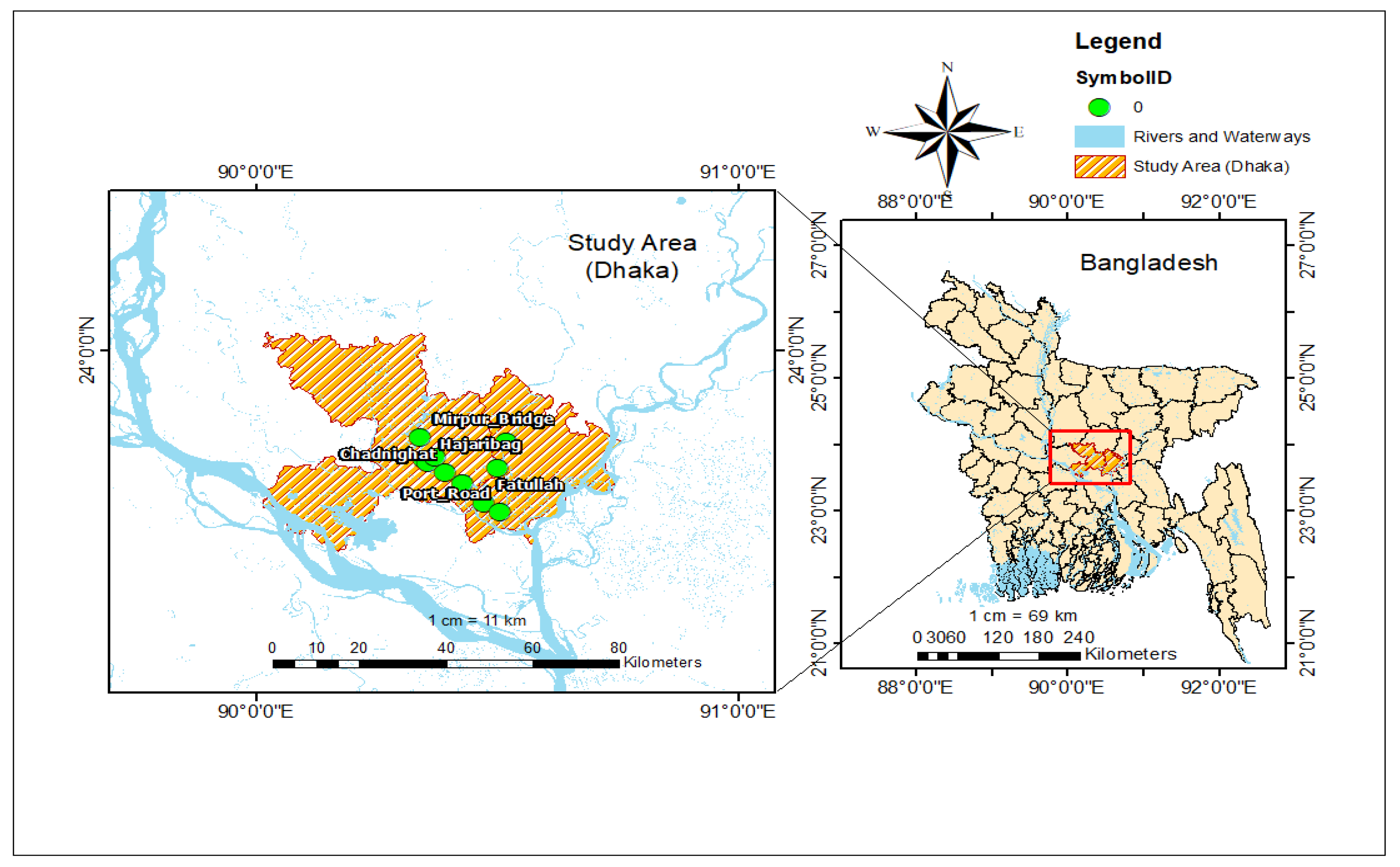
This study focuses on three major rivers (Figure 2): Buriganga, Shitalakhya, and Turag, which form an integral part of Dhaka’s hydrological network and play a crucial role in maintaining the city’s socio-economic and ecological stability. Urbanization, industrial discharge, and waste inflow severely affect these rivers, making them crucial for monitoring and managing water quality. The Buriganga River originates from the Dhaleshwari River near Kalatia (approx. 23°40′55″ N, 90°25′10″ E) and flows along the southern edge of Dhaka before discharging back into the Dhaleshwari near Hasnabad. Its estimated basin area is about 253 km2, with an average flow ranging from 150 m3/s to 1119 m3/s during peak monsoon. The Shitalakhya River branches off from the old Brahmaputra River near Mymensingh and flows southward through Narsingdi and Narayanganj, finally joining the Dhaleshwari near Kalagachhia (approx. 23°34′11″ N, 90°32′00″ E). The river covers a basin area of roughly 624 km2, with an average discharge varying seasonally from 330 m3/s to 1593 m3/s. The Turag River originates from the Bangshi River near Gazipur (approx. 23°45′59″ N, 90°19′60″ E) and flows south along Dhaka’s western boundary, merging with the Buriganga near Mirpur. The basin area of the Turag is approximately 1160 km2, and its average discharge ranges from 124 m3/s during dry periods to 1136 m3/s in monsoon months.
Figure 2.
Case study location.
Water quality data were collected from 17 monitoring stations distributed along the three rivers. A total of 476 datasets were utilized in this study, comprising monthly observations recorded between January 2021 and December 2023. The data were obtained from validated sources, including the Department of Environment (DoE) (https://doe.gov.bd/pages/publications, accessed on 1 January 2026) and the Bangladesh Water Development Board (BWDB) (http://www.hydrology.bwdb.gov.bd/, accessed on 1 January 2026). In addition, real-time data were collected from multiple as well as corresponding locations and verified through laboratory testing to ensure cross-checking of the entire dataset. Each observation comprised 15 key physicochemical parameters (Table 1), including pH, dissolved oxygen (DO), biochemical oxygen demand (BOD), chemical oxygen demand (COD), total dissolved solids (TDS), turbidity, chloride, suspended solids (SS), alkalinity, and others. These parameters were selected to comprehensively evaluate the overall river water quality. The corresponding testing methods, units of measurement, and analytical instruments used for each parameter are also summarized in Table 1. to ensure methodological transparency and reproducibility. The dataset comprises physicochemical water quality indicators that are routinely monitored by regulatory agencies and directly influence seasonal water quality variability. Biological parameters were not consistently available during the study period and therefore could not be included. As a result, the developed models primarily capture physicochemical controls on seasonal water quality dynamics rather than the full biotic functioning of the river ecosystem. While biological indicators are critical for directly assessing eutrophication, cyanobacterial blooms, and pathogen-related drinking water risks, the present framework provides a robust physicochemical baseline for seasonal water quality assessment and management.
Table 1.
Parameter descriptions and testing methods.
2.3. Data Preparation and Processing
To ensure comprehensive data preprocessing and cleaning were performed prior to model development. Missing values were handled using mean and median imputation, while inconsistent data entries—including misspellings, improper capitalization, and non-uniform naming conventions—were corrected to improve overall data consistency and enhance model stability and generalization. Outliers in the physicochemical dataset were identified using the IQR method, which is well suited for non-normally distributed environmental data. For each numeric feature, the first quartile (Q1) and third quartile (Q3) were calculated, and the IQR was determined as IQR = Q3 − Q1. Values lying below Q1 − 1.5 × IQR or above Q3 + 1.5 × IQR were flagged as potential outliers. These identified outlier rows were manually removed to prevent extreme values from biasing correlation analysis and ML model performance, while preserving the overall data distribution. Therefore, all observations were retained to preserve the natural variability of the system. Multicollinearity among predictor variables was assessed using Variance Inflation Factor (VIF) analysis, which indicated moderate to high collinearity among certain features. However, because tree-based models (e.g., RF, XGBoost) are inherently robust to multicollinearity, all predictor variables were retained in the modeling process unless they were considered non-essential from a physicochemical perspective. This approach ensured that the feature set remained both scientifically meaningful and statistically stable. All continuous variables were normalized using min–max scaling to maintain uniformity in feature magnitudes and optimize model performance. The dataset was then categorized into four seasonal labels, Winter (December–February), Pre-Monsoon (March–May), Monsoon (June–September), and Post-Monsoon (October–November), based on the respective data collection months. To prevent data leakage, all preprocessing steps, including normalization and feature transformation, were applied after dividing the dataset into training and testing subsets. All data preprocessing, visualization, and classification modeling were conducted using Jupyter Notebook 7.2.2, an open-source interactive computing platform that supports collaborative and reproducible machine learning workflows (https://jupyter.org/, accessed on 1 January 2026).
2.4. Model Development
This study uses three distinct machine learning algorithms, RF, DT, and XGBoost, to create a model for predicting seasonal variations in river water. Based on their proven abilities and strengths in handling prediction and classification problems, RF, DT, and XGBoost were chosen from among the other methods. More specifically, RF effectively manages imbalanced and nonlinear interactions and offers reliable forecasts. RF is a good option for seasonal variation prediction since it can handle a variety of input data and capture intricate relationships between variables. DT can handle both numerical and categorical data and are easily interpretable. Additionally, DT are suitable for tasks involving the prediction and optimization of seasonal variations, particularly when understanding the underlying decision-making process is essential. To achieve high predicted accuracy, XGBoost combines the advantages of gradient boosting and decision trees.
2.4.1. Random Forest (RF)
One popular supervised machine learning technique that works well for regression and classification problems is RF. In order to create a forest, it builds several decision trees using an ensemble technique. The forecasts from each individual tree are combined to form the forest’s final forecast. This aggregation improves accuracy by reducing overfitting problems that are frequently seen with decision tree algorithms such as gradient-boosted trees. Measures of entropy and information gain are applied in feature selection. A favorable feature is one that has a higher information gain and a lower entropy [38]. This suggests that the feature offers more useful data for the classification task, improving the RF algorithm’s overall performance.
2.4.2. Decision Tree (DT)
One well-known machine learning technique for prediction and classification is called DT, which speeds up decision-making in various decision-making situations. In many real-world situations, DT and decision rules form the basis of data mining applications, providing a potent remedy for categorization issues. Regression trees and classification trees are two categories into which DT can be divided based on the kind of output variable. Based on the output variable, a classification tree was considered in this study. Building a model that allocates suitable values of the output variable to the input variables of an item is the main goal of categorization. Classifying the output variables into classes or categories is the primary goal of a DT model [39].
2.4.3. Extreme Gradient Boosting (XGBoost)
XGBoost is a nonprobability classifier and an improved distributed gradient improvement library that enhances the gradient lifting algorithm [40]. It is an ensemble learning method based on gradient-boosted decision trees, designed to achieve high predictive accuracy through iterative optimization. In this study, it was employed for multi-class classification using a tree-based boosting framework. The model minimizes a differentiable loss function, while regularization techniques—including L1/L2 penalties, tree depth constraints, and minimum child weight—prevent overfitting. Row-wise and feature-wise subsampling were applied to enhance generalization, and class imbalance was addressed through weighted training. The loss function’s extreme values are solved using the Newton method after a second-order Taylor expansion, incorporating the regularization term. XGBoost is widely recognized for its efficiency, flexibility, and reliability in classification tasks.
2.5. SHapley Additive exPlanations (SHAP)
SHAP is a model-agnostic interpretation method grounded in cooperative game theory that explains how each feature contributes to a model’s prediction. It utilizes Shapley values to fairly distribute the model output among features by calculating their average marginal contributions across all possible feature combinations [41]. SHAP provides both global and local interpretability, ensuring consistency and transparency in model explanations. It is particularly effective for tree-based models, such as RF and XGBoost, through the efficient TreeSHAP algorithm. In this study, SHAP analysis was applied to identify the relative importance of each parameter and to assess how individual features influenced the model’s predictions. This approach quantifies the extent to which each feature alters the output, thereby enhancing understanding of feature significance and model behavior.
2.6. Partial Dependence Plots (PDP)
By measuring the marginal impact of one or more input variables on the desired outcome, partial dependence plots (PDPs), which are model-agnostic visualization tools, are used to evaluate machine learning predictions. PDPs provide information on feature relevance and model behavior by displaying whether the relationship between features and predictions is linear, monotonic, or very nonlinear. While marginalizing other variables, the average prediction over all observations isolates the contribution [42]. The model’s sensitivity to that variable is indicated by the PDP curve’s slope or curvature; steeper gradients signify greater influence. PDPs were used in this work to assess the distinct impacts of the most crucial river water parameter. In addition to identifying important variables, this study makes sophisticated nonlinear machine learning models used to predict seasonal variation interpretable.
2.7. Model Hyper-Parameter Optimization and Model Performance
RandomizedSearchCV-based hyperparameter optimization and 5-fold cross-validation (CV) were performed for all ML algorithms to ensure methodological transparency and minimize model selection bias. Initially, the dataset was divided into 80% for training and 20% for testing to evaluate the model’s generalization on unseen data. Within the training phase, a 5-fold CV was applied, where the data were further partitioned into five equal subsets; in each iteration, four folds were used for training and one for validation. Each fold served once as the validation set, and the process was repeated five times. By averaging the results across all folds, this approach mitigates bias from a single train–test split and provides a robust estimate of the model’s predictive performance. Consequently, the reported performance metrics (precision, recall, F1-score, and accuracy) represent the mean ± standard deviation across the five folds, offering a statistically reliable evaluation of model generalization. Table 2. summarizes the optimal hyperparameters for each model, obtained through systematic parameter tuning to balance predictive accuracy and overfitting control.
Table 2.
Optimal hyperparameters for ML models.
2.8. Model Performance Test
2.8.1. Classification Report
A range of evaluation indicators should be considered to comprehensively assess the performance of ML classification models. Accuracy is one of the most common metrics used to measure predictive performance. It shows the percentage of samples that were correctly predicted out of the total number of samples. A higher value means better predictive performance. The F1-score represents the harmonic mean of precision and recall, which are complementary measures—an increase in recall often results in a decrease in precision, and vice versa. The mathematical expressions for calculating accuracy, precision, recall, and F1-score are presented in Equations (1)–(4) [43].
where FP stands for false positive, TN for true negative, FN for false negative, and TP for true positive (i.e., the number of correctly categorized positive samples).
2.8.2. ROC Curve and AUC
The true positive rate (TPR) is plotted on the y-axis and the false positive rate (FPR) on the x-axis in a graphical representation known as the ROC curve. The trade-off between coverage and accuracy is shown by this graph. High accuracy and coverage are indicated by an FPR that is near 0 and a TPR that is near 1. One metric that measures the classifier’s capacity to differentiate between samples is the AUC. Classifier performance is often assessed using the AUC value, which is insensitive to the balance of sample classes. A better classifier performs better when its AUC score is larger.
3. Results
3.1. Correlation Analysis
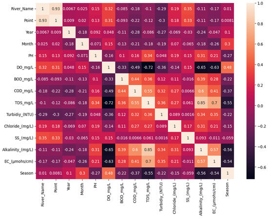
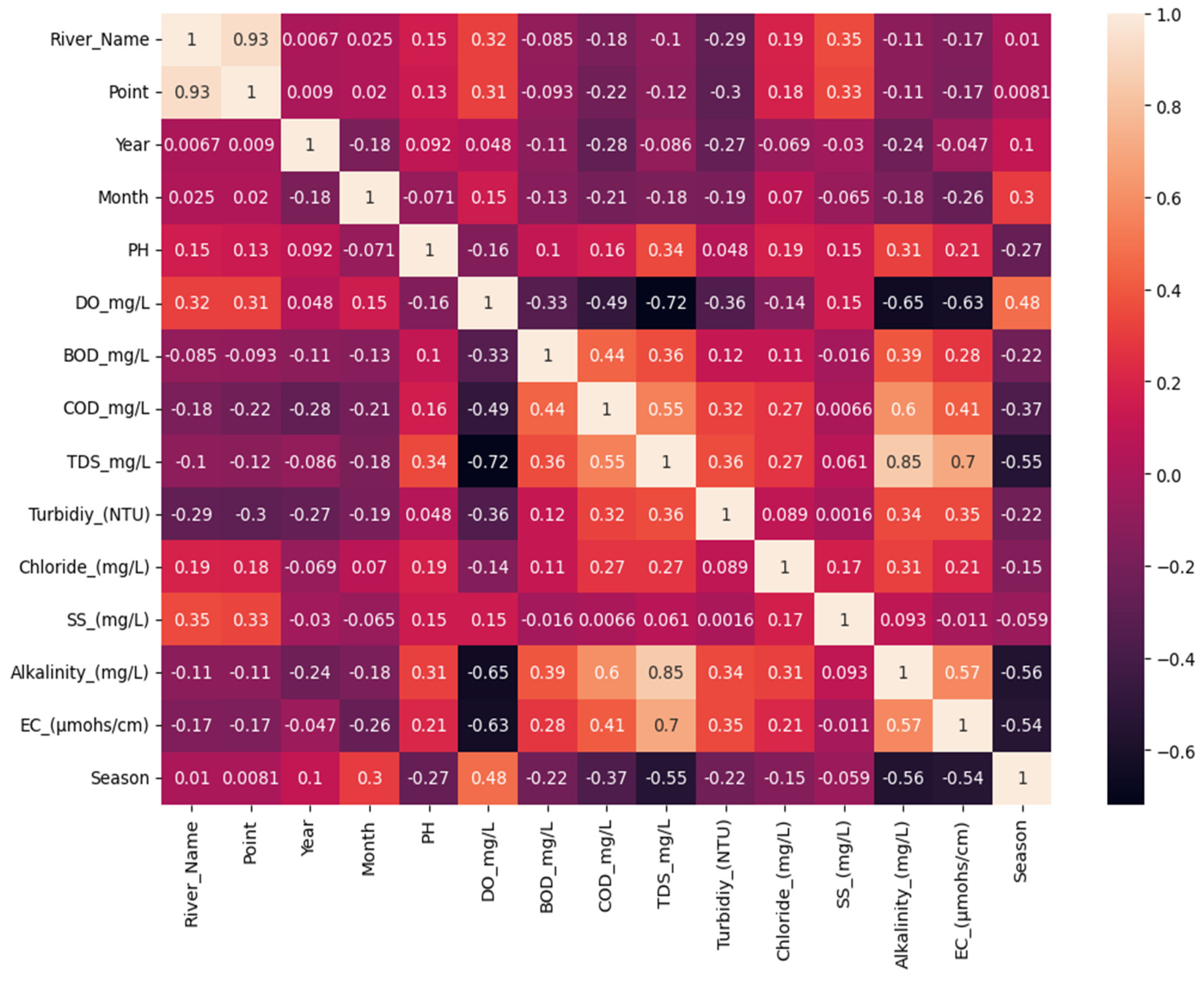
Figure 3 presents a heatmap illustrating the correlations among various water quality parameters. This correlation analysis served as an initial diagnostic tool to identify potential multicollinearity within the physicochemical variables. To further validate these findings and quantify the extent of multicollinearity, the corresponding VIF results are provided in Appendix A. Notably, strong positive correlations were observed between TDS and EC (r = 0.85), as well as between TDS and alkalinity (r = 0.55), suggesting possible redundancy among ionic-related parameters. In the same way, COD also shows a positive relation with TDS (r = 0.60) and BOD (r = 0.44). This means both organic and inorganic pollution are connected and mostly come from the same pollution sources. On the other hand, DO shows a strong negative relation with TDS (r = −0.72) and COD (r = −0.49). It means when the pollution level goes high, the dissolved oxygen in water goes down. Also, DO and EC (r = −0.63) have a negative relation, which shows oxygen level decreases when ionic concentration increases in the river. Season also shows a negative relation with TDS, EC, and alkalinity (around −0.55). This phenomenon may happen because during rainy season or monsoon time, rainwater causes dilution and reduces this value. A moderate positive relation was found between alkalinity and TDS (r = 0.55) and also with EC (r = 0.57). This indicates that carbonate and bicarbonate ions primarily contribute to the increase in these parameters. Turbidity and Suspended Solids (SS) (r = 0.34) also have a positive relation, which is normal because when solid particles increase, water becomes more turbid. Some parameters, like pH, month, and year, show very weak or no relation with other factors. Overall, this correlation analysis shows that DO, TDS, EC, and COD are the main important parameters that affect river water quality. Seasonal changes also play a big role in these water parameters.
Figure 3.
Correlation matrix heatmap of 15 features.
3.2. Classification Report and Confusion Matrix
Table 3 presents the comparative classification performance of the three machine learning models, RF, XGBoost, and DT for predicting the seasonal class. Among the evaluated models, RF achieved the highest overall performance, with precision, recall, F1-score, and accuracy all equal to 0.79, indicating strong and balanced predictive capability. XGBoost followed closely, obtaining precision and recall values of 0.77 and an F1-score of 0.76, while DT performed comparatively lower with all metrics at 0.74. These results confirm that RF exhibits superior generalization and class discrimination ability, making it the most accurate model for seasonal classification tasks. The results demonstrate that ensemble-based models, particularly RF, outperform single-tree classifiers due to their enhanced capability to reduce overfitting and variance through bootstrap aggregation and random feature selection. These findings align with previous studies, which reported that ensemble learners such as RF and XGBoost generally achieve higher robustness and generalization in environmental and climatic classification tasks compared to conventional decision trees [40,44,45]. The training dataset evaluation metrics for all models are provided in detail in Appendix B.
Table 3.
Model performance of three ML models.
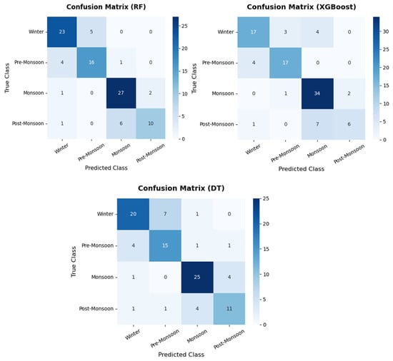
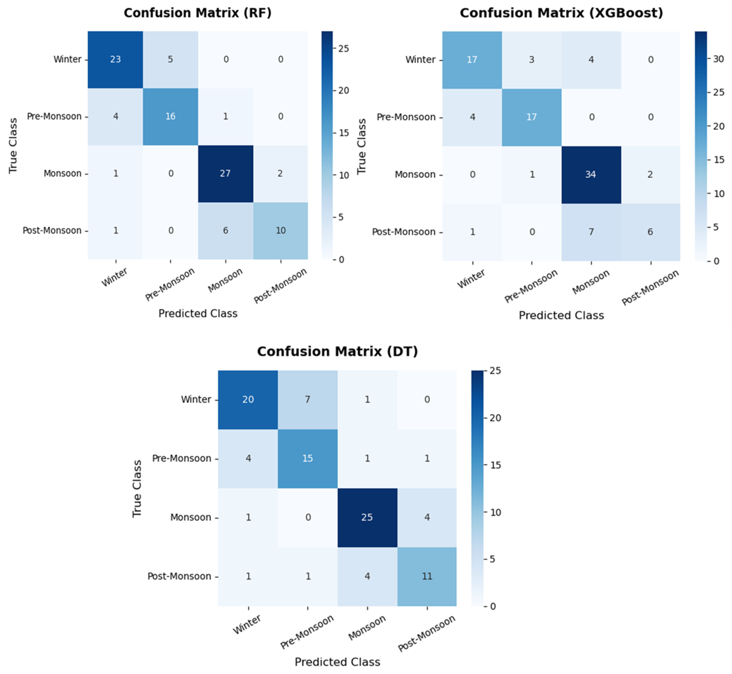
Confusion matrices are applied to analyze the ML models’ performance per class, allowing for insight beyond overall accuracy. The confusion matrices indicate that all three models exhibited consistent and reliable performance in classifying seasonal variations in river water quality. Each matrix shows how the actual and predicted classes compare, which makes it possible to fully assess the model’s accuracy and trends in misclassification. The confusion matrices presented in Figure 4 illustrate the classification performance of the three ML models, RF, DT, and XGBoost, in the prediction task. The RF model exhibited a high degree of accuracy across all seasonal classes, particularly for the monsoon (27 correctly classified) and winter (23 correctly classified) seasons, indicating robust generalization and minimal misclassification. The pre-monsoon class showed a moderate performance, with most instances correctly classified. The XGBoost model achieved the highest accuracy for the monsoon season (34 correct predictions), reflecting its strong capacity to capture non-linear relationships and feature interactions. However, minor misclassifications were observed between the winter and pre-monsoon categories and between monsoon and post-monsoon, suggesting partial seasonal transition overlap in the dataset. Conversely, the DT model exhibited comparatively lower overall accuracy, with noticeable confusion between winter and pre-monsoon, and between monsoon and post-monsoon. Although the model captured major seasonal trends, its simpler structure likely limited its ability to differentiate complex intersessional patterns. The limited misclassifications observed between pre-monsoon and winter for the RF model, and between monsoon and post-monsoon for the XGBoost model, can be explained by hydrometeorological continuity across seasonal transitions. In the study area, pre-monsoon and winter periods often share relatively low rainfall, reduced river discharge, and stable flow conditions, resulting in similar physicochemical signatures such as elevated dissolved oxygen and comparatively lower turbidity and suspended solids. Likewise, monsoon and post-monsoon seasons exhibit overlapping hydrological characteristics due to residual monsoonal rainfall, delayed recession of river flow, and continued catchment runoff. These transitional hydrometeorological conditions lead to partial overlap in water quality parameter distributions, which can cause limited class confusion despite the overall high predictive performance of the models. Such behavior reflects realistic seasonal dynamics rather than model inadequacy. Overall, the comparative analysis of the confusion matrices highlights that RF and XGBoost outperform DT in capturing seasonal variability, with RF demonstrating better balance across all classes, while XGBoost achieved superior precision in the monsoon classification.
Figure 4.
Confusion matrix for season prediction.
3.3. ROC–AUC Curve Report
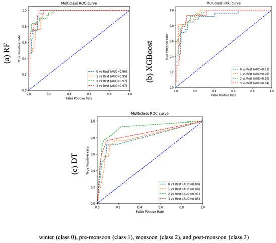
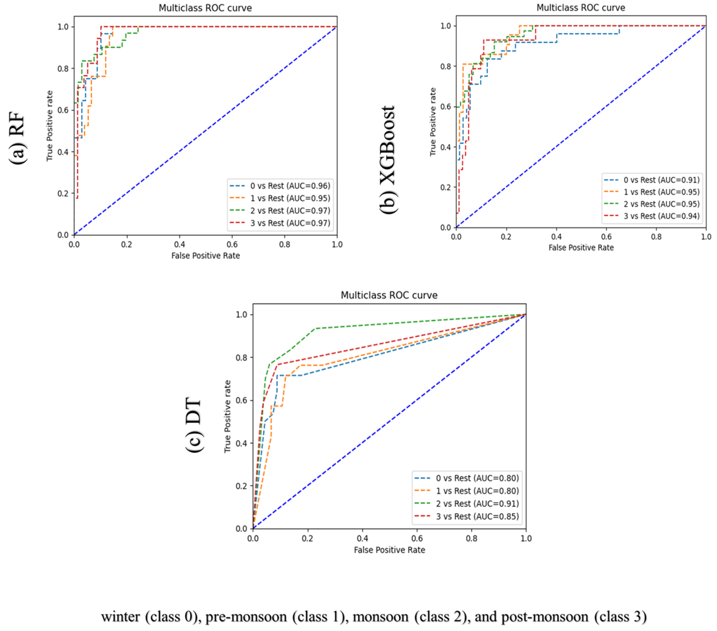
The ROC curves presented in Figure 5 illustrate the classification performance of three ML models, RF, XGBoost, and DT, for predicting the seasonal variations in river water quality across four distinct periods: winter (class 0), pre-monsoon (class 1), monsoon (class 2), and post-monsoon (class 3). The AUC values were used as the principal metric to evaluate the discriminative ability of each model.
Figure 5.
AUC-ROC for (a) RF; (b) XGBoost; (c) DT models for seasonal classification.
The RF model demonstrated (Figure 5a) superior classification capability, achieving AUC values of 0.96, 0.95, 0.97, and 0.97 for winter, pre-monsoon, monsoon, and post-monsoon, respectively. These results indicate excellent model performance with consistent accuracy across all seasonal classes. The XGBoost model also exhibited (Figure 5b) high predictive accuracy, with AUC values of 0.91 (winter), 0.95 (pre-monsoon), 0.95 (monsoon), and 0.94 (post-monsoon), confirming its robustness and stability in capturing non-linear seasonal dependencies. Conversely, the DT model (Figure 5c) produced relatively lower AUC values of 0.80, 0.80, 0.91, and 0.85 for the corresponding seasons, reflecting its limited capacity to model complex relationships compared to ensemble-based approaches.
Overall, ensemble algorithms such as RF and XGBoost significantly outperformed the single-tree model, underscoring the effectiveness of ensemble learning in capturing intricate physicochemical and hydrological interactions influencing seasonal water quality variations. The consistently high AUC values during the monsoon and post-monsoon periods further suggest enhanced model sensitivity in detecting pronounced seasonal transitions, likely driven by increased runoff, dilution, and changes in dissolved ionic concentration. These findings reaffirm the suitability of ensemble ML techniques for environmental prediction tasks, offering superior generalization and interpretability in comparison to conventional models. Similar observations have been reported in contemporary research on AI-driven water quality modeling [46,47].
3.4. SHAP Analysis of Feature Importance
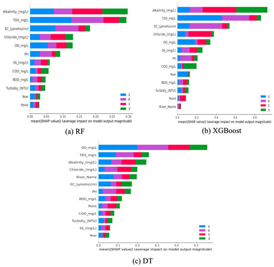
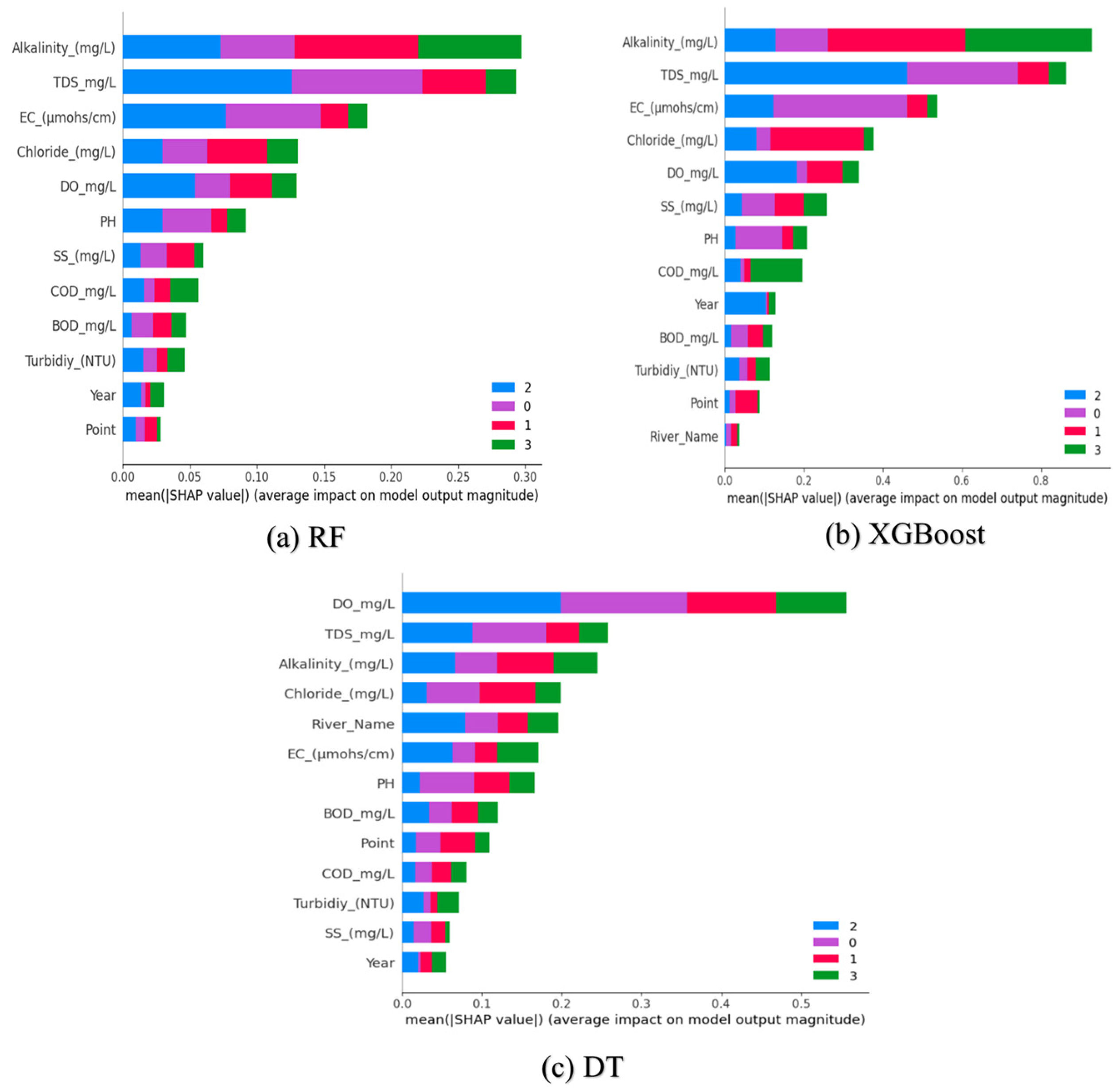
The SHAP analysis was applied to interpret and rank the relative contribution of physicochemical parameters in predicting the seasonal variations in river water quality. The SHAP summary plot (Figure 6a) indicates that alkalinity, TDS, and EC exhibit the highest mean absolute SHAP values, highlighting their primary influence on the RF model’s predictive performance. These parameters mainly represent the ionic composition and electrical conductivity of water, which fluctuate with seasonal hydrological processes such as rainfall, runoff, and evaporation. Moderate importance was found for chloride, DO, and pH, while SS, COD, and BOD contributed less, indicating that the AI model is more responsive to dissolved ionic and conductivity parameters than to organic or suspended load indicators [46].
Figure 6.
SHAP summary plots for (a) RF; (b) XGBoost; (c) DT models.
Similarly, the XGBoost model (Figure 6b) revealed that alkalinity, TDS, and EC were the most influential variables, emphasizing their strong predictive power in capturing seasonal dynamics of river water quality. These features reflect the ionic strength and salinity characteristics of the aquatic environment, which are highly sensitive to hydrological cycles, such as dilution during monsoons and concentration during dry periods. Chloride, DO, and SS exhibited moderate SHAP contributions, suggesting that the model also accounts for dissolved oxygen and sediment-related processes to a limited degree. Lower-ranked parameters such as COD, BOD, turbidity, and year exerted minimal influence, supporting the consistency of findings between RF and XGBoost in identifying conductivity-related parameters as primary seasonal drivers.
In contrast, the DT model (Figure 6c) displayed a slightly different ranking pattern, where DO emerge as the most influential predictor, followed by TDS, alkalinity, and chloride. This deviation may be attributed to the inherent structure of the DT algorithm, which relies on a single, non-ensemble tree that tends to emphasize features with strong threshold-based separability rather than cumulative variable interactions.
Consequently, DT prioritized DO, a parameter with clear seasonal thresholds between wet and dry conditions, over conductivity-related features. River name and EC also showed notable SHAP values, reflecting site-specific and ionic effects on water quality prediction. Parameters such as pH, BOD, and COD contributed minimally, while SS and year were least influential.
The SHAP-based interpretation consistently revealed that ionic and conductivity-related parameters predominantly govern the seasonal variation in river water quality across all three models. This finding aligns with previous studies by Schäfer et al. [48], Yang et al. [49], and Wang et al. [50], which similarly emphasized the strong influence of ionic composition and conductivity on spatiotemporal water quality dynamics. However, the slight divergence observed in the DT results underscores that ensemble-based models such as RF and XGBoost provide more stable and generalizable feature attributions compared to single-tree methods. This consistency further confirms the robustness of SHAP analysis in interpreting complex water quality datasets.
3.5. Partial Dependence Plot (PDP)
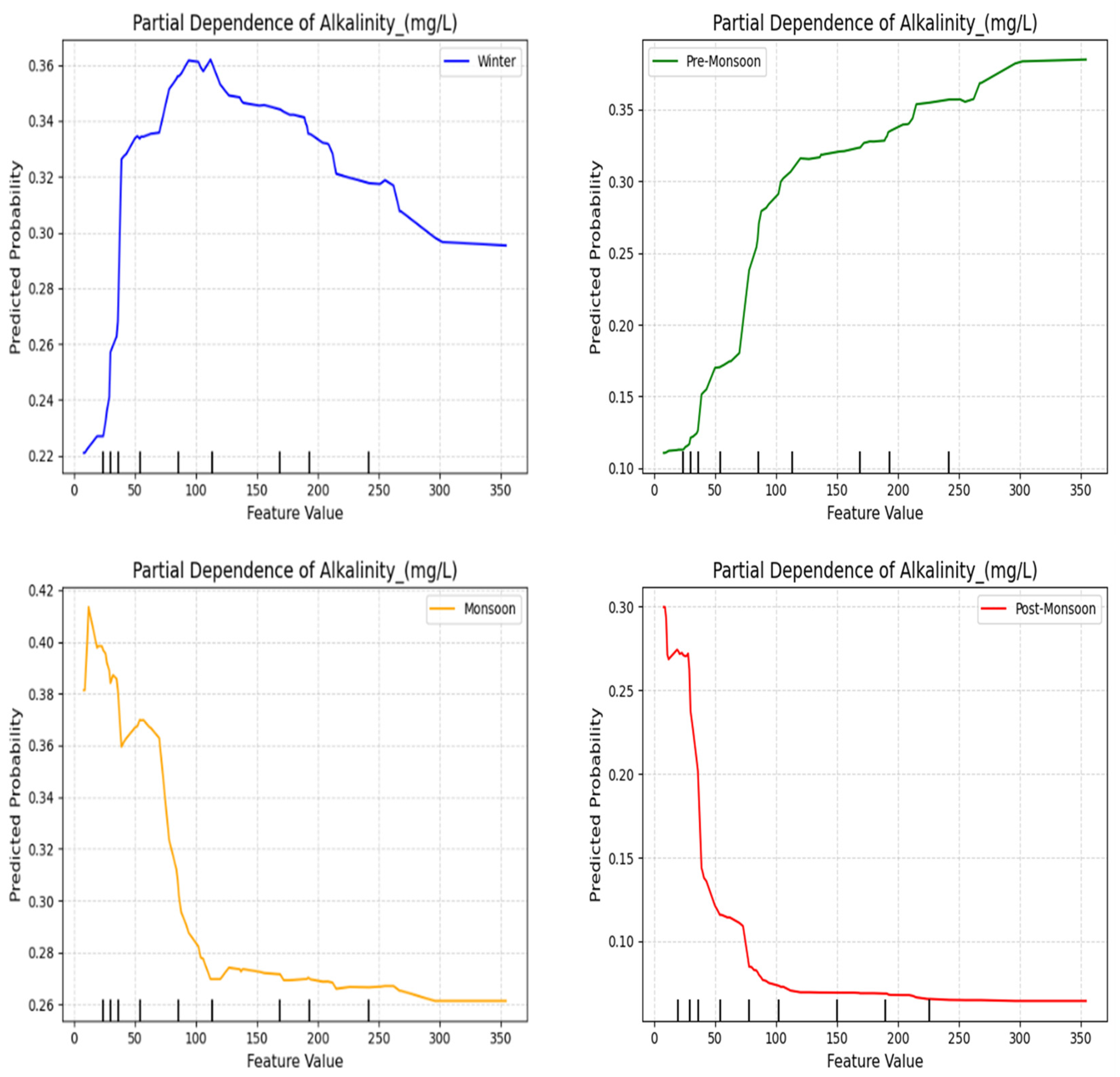
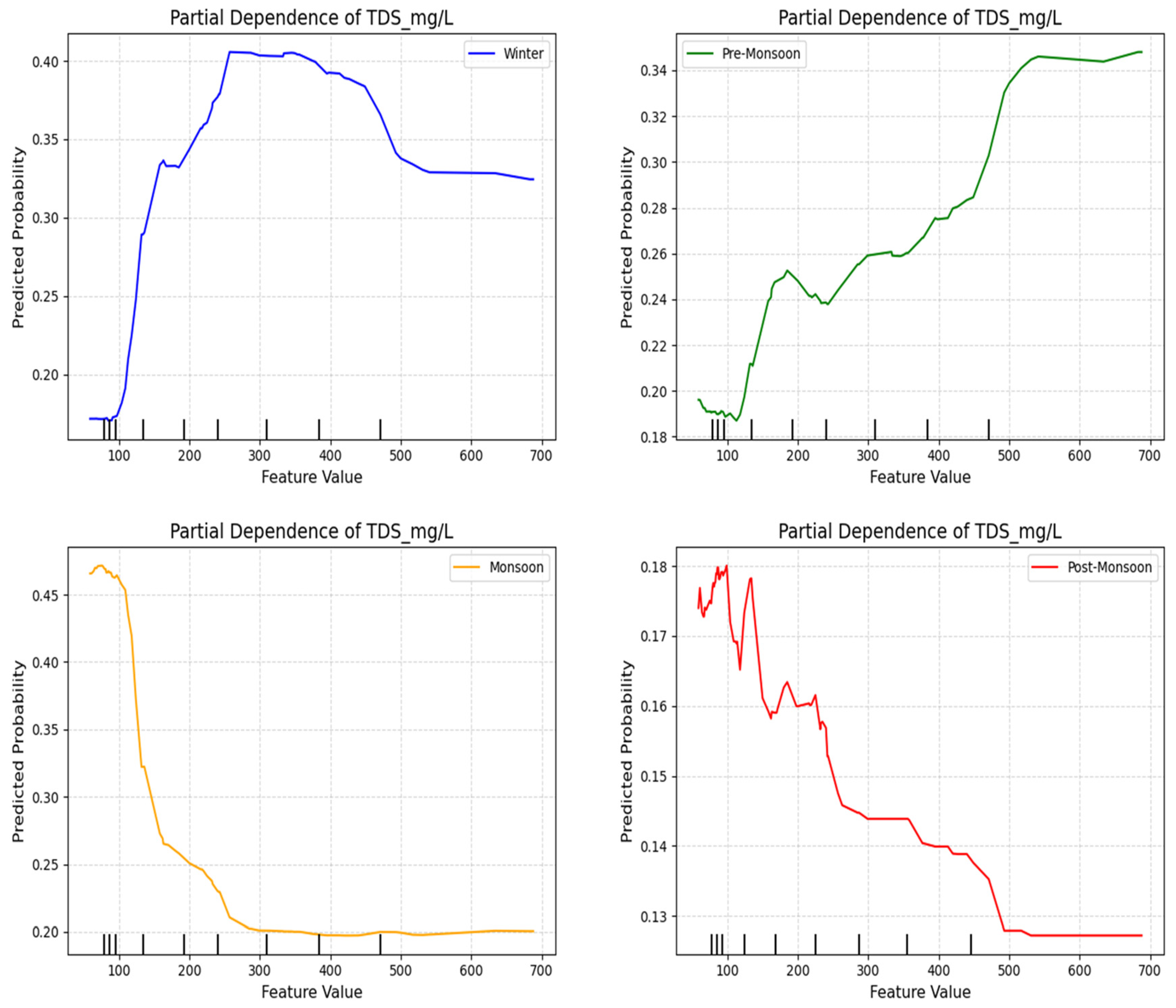
Partial Dependence Plot (PDP) analysis was employed to examine the sensitivity of the top-ranked influential features to seasonal variations while holding less important variables constant. Based on the SHAP feature importance ranking, three primary predictors, alkalinity, TDS, and EC, were selected for PDP analysis. The analysis illustrates the marginal effects of each parameter on seasonal classification probabilities across four distinct categories—winter, pre-monsoon, monsoon, and post-monsoon—thereby quantifying their individual influence on the model outputs. Correspondingly, Table 4 summarizes the PDP results, presenting the lower and upper bounds, minimum and maximum PDP outputs, and the computed range (Δ) for each feature across different seasons, which collectively elucidate the extent of variation and sensitivity of each predictor under varying seasonal conditions.
Table 4.
PDP-based evaluation for Alkalinity, TDS, and EC.
3.5.1. Alkalinity
As shown in Figure 7, the predicted probability of winter and pre-monsoon increased consistently with alkalinity, rising from approximately 0.22 to 0.36 within the 0–100 mg/L range. This suggests enhanced buffering capacity and carbonate equilibrium stability during dry seasons when river discharge is minimal. Conversely, during monsoon and post-monsoon, a downward trend was observed beyond 50 mg/L due to dilution effects from rainfall and surface runoff. This reversal (Δ ≈ 0.16) demonstrates the strong seasonal dependence of alkalinity dynamics. Similar findings were reported by Uddin et al. [51] reported similar findings, noting reduced alkalinity during monsoon due to enhanced freshwater inflow in coastal Bangladesh rivers.
Figure 7.
PDP of Alkalinity (mg/L) showing model-predicted probability across four seasons.
3.5.2. Total Dissolved Solids (TDS)
The PDP for TDS (Figure 8) revealed a strong non-linear relationship with predicted seasonal probabilities. Winter and pre-monsoon probabilities increased sharply from 100 to 300 mg/L, reflecting solute accumulation due to evaporation and reduced flow, and then plateaued beyond 300 mg/L. In contrast, monsoon and post-monsoon probabilities decreased after 100 mg/L, suggesting strong dilution during peak rainfall. The total response amplitude (Δ ≈ 0.25) indicates TDS as the most responsive parameter to seasonal hydrological shifts. This agrees with Islam et al., [52], who reported similar pre-monsoon TDS peaks followed by monsoonal dilution in Dhaka’s rivers.
Figure 8.
PDP of TDS (mg/L) showing model-predicted probability across four seasons.
3.5.3. Electrical Conductivity (EC)
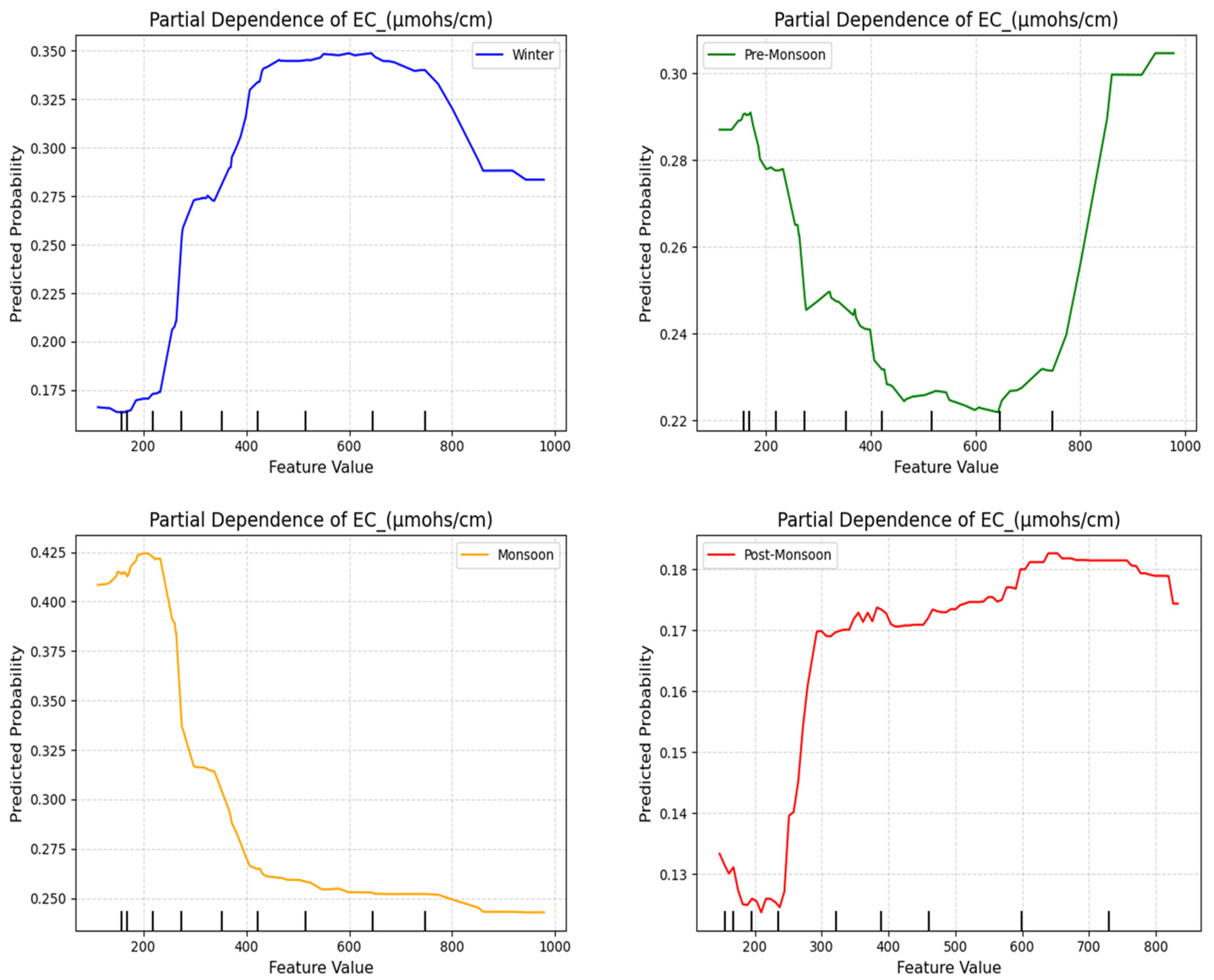
The PDP for EC is shown in Figure 9. The EC (112–978 µmhos/cm) showed a moderate influence on predicted probability (Δ ≈ 0.18) and revealed distinct seasonal patterns: higher probabilities associated with higher EC during the dry season (winter), implying ionic retention/salt intrusion, and lower probabilities during the wet season (monsoon), consistent with dilution by rainfall. Comparatively, a recent study by Assessment of physicochemical properties of water and their seasonal variation in an urban river in Bangladesh. Rahman et al. found that EC varied markedly between dry and wet seasons in an urban Bangladeshi river setting (EC ranged ~110–910 µS/cm) with lowest values in the wet season [53]. Thus, our findings align with previous local work insofar as EC increases during lower-flow/dry periods and decreases during high-flow/wet periods, reinforcing the interpretation that EC serves as a proxy for solute concentration dynamics under changing hydrological conditions.
Figure 9.
PDP of EC (µmhos/cm) showing model-predicted probability across four seasons.
4. Discussion
4.1. Comparative Performance and Explainability of ML Models Across Seasonal River Conditions
Seasonal river water quality in highly urbanized catchments is governed by complex interactions among hydrological variability, pollutant loading, and physicochemical processes. The observations analyzed in this study reflect routine seasonal and interannual fluctuations in river conditions, including rainfall-driven changes in flow that influence turbidity, suspended solids, and organic pollution indicators. In this broader context, Dhaka and Gazipur have been among the most flood-affected regions in Bangladesh in terms of inundation extent and exposed population, providing an important hydrological backdrop for understanding the observed variability in river water quality [54]. However, samples collected during extreme hydro-meteorological events (e.g., peak flood or disaster-period conditions) were not intentionally included, as all measurements were obtained during standard monitoring periods. Consequently, the developed machine learning models are most applicable for characterizing and predicting seasonal variation dynamics under typical hydrological conditions rather than extreme climate scenarios. This distinction is important when interpreting seasonal overlap in physicochemical characteristics and occasional misclassification between adjacent seasons.
Among the evaluated models, the RF model achieved the highest predictive accuracy (79%), followed by XGBoost (77%) and DT (74%), demonstrating robust generalization across nonlinear physicochemical relationships. Rachid et al. predicted water potability using an ML approach, reporting that the RF outperformed the SVM model with 70% accuracy, 72% precision, and a 75% ROC–AUC [55]. In contrast, the present study focuses on predicting seasonal variations in river water quality using an ML approach that integrates multiple physicochemical parameters. The results demonstrate superior predictive performance, indicating improved accuracy, robustness, and reliability over previous findings. Compared to Hasikin et al., who achieved 77.68% using a modified RF model [56], and El Hafyani et al., whose multi-view stacking model achieved superior performance in precipitation forecasting [57], the present RF framework demonstrates superior balance among precision, recall, and F1-score across seasonal classes, underscoring its reliability under hydrologically dynamic and data-limited conditions. A key strength of this study lies in combining SHAP and PDP analyses, which provide explainable, feature-level interpretations, revealing that alkalinity, TDS, and EC are the dominant drivers of seasonal variation. Such interpretive transparency remains absent in most earlier studies [46].The ensemble model demonstrated exceptional predictive power, achieving an AUC above 0.95 for all seasonal classes. This performance clearly outperforms comparable explainable AI frameworks, such as those developed by Nallakaruppan et al. [47] and Yang et al. [49], whose reported AUC values remained below 0.93. These results highlight the model’s superior ability to distinguish water quality variations across seasons and confirm its reliability for practical river-management applications. Unlike prior single-river or static WQI models [1,37,50], this study integrates multi-river data (Buriganga, Shitalakhya and Turag), addressing spatial heterogeneity and enhancing model generalizability. Data for this study were collected from 17 monitoring stations, which provides a broader spatial coverage compared to the study by Del Castillo et al., who collected data from 6 to 13 monitoring sites to predict river water quality [8]. Moreover, the study validates the dominance of ionic and conductivity-related parameters, corroborating Schäfer et al. [48], while extending their insights through cross-seasonal and multi-river explainability.
Hence, this research advances the frontier of explainable ensemble AI for sustainable water quality assessment, combining predictive strength with mechanistic interpretability rarely achieved in the prior literature. From a management and regulatory perspective, the achieved classification accuracies (RF: 79%; XGBoost: 77%; DT: 74%) have clear practical significance for water quality assessment. These performance levels indicate that the models can reliably distinguish seasonal pollution regimes associated with variations in key physicochemical indicators that are commonly evaluated against guideline-based thresholds defined by WHO and national surface water quality standards of Bangladesh. For example, dissolved oxygen concentrations below approximately 5–6 mg L−1 are widely recognized as indicative of ecological stress for aquatic life, pH values outside the recommended range of 6.5–8.5 reflect chemical imbalance, BOD levels exceeding ~5 mg L−1 indicate elevated organic pollution, and TDS values approaching or exceeding ~1000 mg L−1 suggest degraded water quality [6,58]. While the proposed framework does not explicitly predict threshold exceedance events, its ability to consistently identify seasonal conditions associated with deterioration in these physicochemical indicators enables effective early warning of potential non-compliance with WHO and Bangladesh water quality guidelines. Consequently, the models provide a valuable decision-support tool for prioritizing field monitoring, identifying high-risk seasons and river reaches, and supporting proactive river-management and pollution-control strategies under hydrologically dynamic conditions.
4.2. AI-Based Seasonal Water Quality Management System
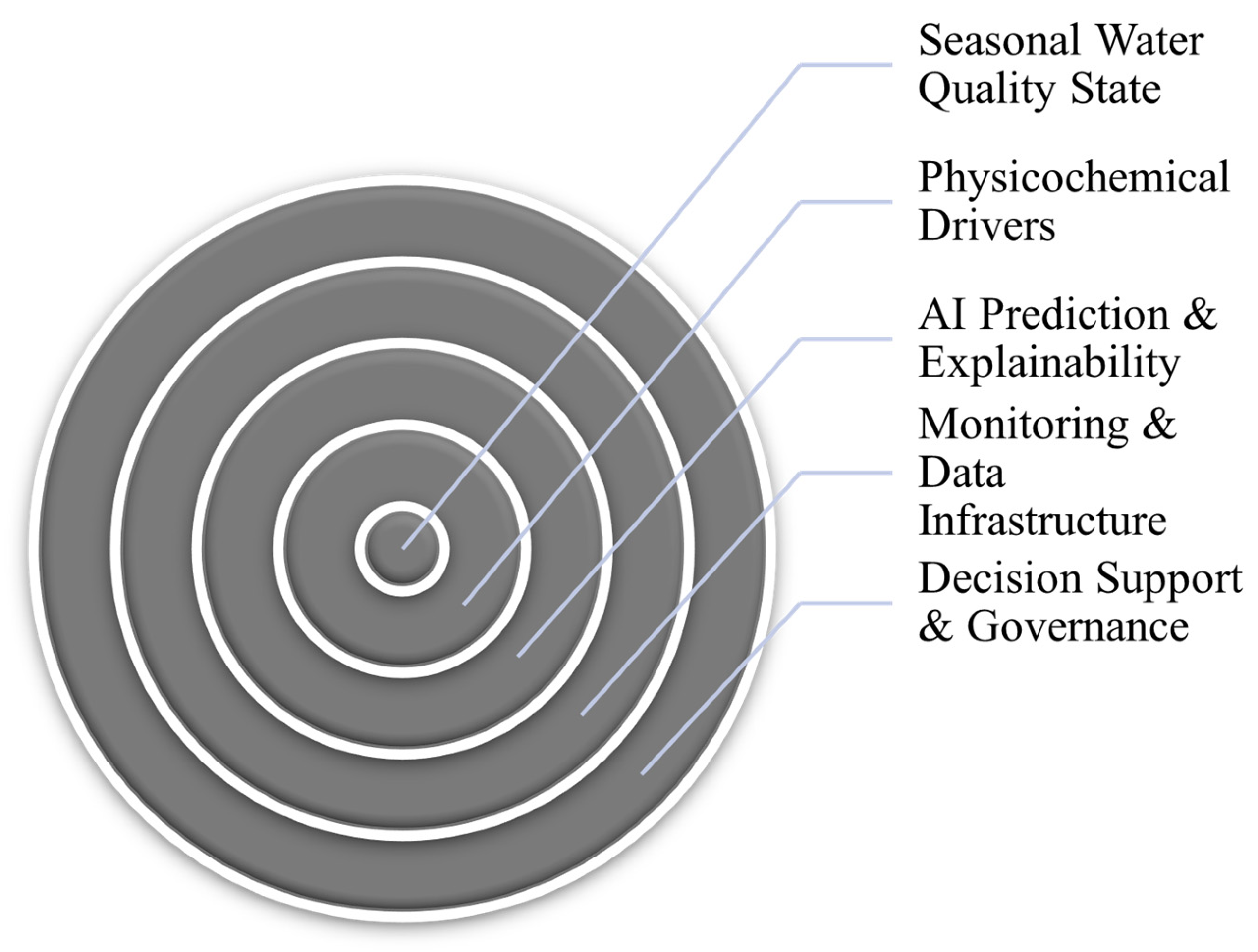
This study presents a holarchy AI-based conceptual framework for assessing and managing seasonal river water quality, as illustrated in Figure 10. The framework is organized as a set of interconnected layers, where each layer performs a specific role while collectively supporting the overall system. In this holarchy structure, individual layers can operate independently, yet they remain closely linked to one another, ensuring smooth information flow from data collection to decision-making. Applied to river water quality management, this approach brings together environmental monitoring, machine learning–based analysis, model interpretability, and management actions into a single, coherent, and scalable system that is easy to understand and practical to apply.
Figure 10.
Conceptual AI-Based Seasonal Water Quality Framework illustrating the integration of seasonal physicochemical inputs and machine learning prediction.
At the center of the holarchy system lies the seasonal water quality state, which represents the final outcome of the framework. This layer divides the quality of river water into four seasonal groups: winter, pre-monsoon, monsoon, and post-monsoon. These groups show the main hydrological and physicochemical conditions that affect river systems in Bangladesh. The core layer summarizes the environmental condition that is most relevant for water resource managers and policymakers, serving as the primary indicator for environmental status assessment.
Surrounding the core is the physicochemical driver layer, which captures the fundamental environmental processes influencing seasonal water quality dynamics. This layer includes key water quality parameters such as alkalinity, TDS, and EC, identified through SHAP analysis as the dominant contributors to seasonal variability. Supporting parameters, including DO, chloride, pH, suspended solids, BOD, and COD, provide complementary information on organic load, ionic composition, and oxygen dynamics. This layer explains the underlying environmental mechanisms responsible for seasonal transitions, such as solute accumulation during dry periods and dilution during monsoon flows.
The third layer consists of the AI-based analytical engine, where ML models process multivariate physicochemical inputs to predict seasonal water quality classes. Ensemble models, particularly RF, capture nonlinear interactions and complex dependencies among parameters, ensuring robust predictive performance. Model explainability is embedded within this layer through SHAP and PDP analyses, enabling transparent interpretation of feature contributions and marginal effects. This layer transforms raw environmental data into understandable knowledge, bridging the gap between prediction accuracy and decision relevance.
The monitoring layer forms the data backbone of the holarchy system. It integrates multi-source water quality data obtained from field measurements, laboratory analyses, and institutional monitoring programs. This layer ensures continuous data flow, quality control, and spatial coverage across multiple rivers and monitoring stations. The framework is inherently scalable, allowing future integration of real-time sensor networks, IoT-based monitoring, and remote sensing data to enhance temporal resolution and operational responsiveness.
The outermost layer represents decision support and governance, where model outputs are translated into actionable insights for environmental management. Seasonal predictions and feature-level explanations inform early-warning systems, seasonal regulation strategies, monitoring prioritization, and pollution control interventions. This layer supports evidence-based policymaking by aligning scientific insights with regulatory actions, enabling adaptive river management under seasonal and climatic variability.
The holarchy structure ensures that each layer operates both independently and cooperatively, allowing localized improvements (e.g., enhanced sensing or model optimization) without disrupting the overall system. By integrating predictive accuracy with explainable intelligence and decision-oriented outputs, the proposed framework moves beyond conventional black-box modeling and establishes a transparent, scalable, and operationally relevant system for seasonal river water quality management. This holarchy AI-based framework is particularly suited for data-limited and hydrologically dynamic regions, offering a practical pathway toward sustainable and adaptive water resource governance. While the proposed AI-based seasonal water quality framework is developed using physicochemical parameters, it is designed as a flexible and modular structure. The framework can be extended to incorporate biological indicators, such as microbial abundance, pathogen-related signals, or organismal response dynamics. This adaptability is particularly important in regions exposed to extreme climatic events, where episodic environmental disturbances may significantly influence aquatic ecosystem behavior.
4.3. Limitations and Future Perspectives
The findings of this study highlight the strong potential of machine learning to capture seasonal river water quality dynamics using routinely monitored physicochemical indicators. The accurate prediction and classification of seasonal conditions demonstrate that the proposed framework can serve as a practical decision-support tool for identifying periods of elevated pollution and areas requiring management attention, emphasizing the value of data-driven models for adaptive, seasonally informed water quality management, particularly in data-limited rivers. Despite these strengths, it is important to acknowledge several limitations. The dataset covers a relatively short period from 2021 to 2023 and lacks real-time or high-frequency sensor data, which may limit the models’ ability to generalize under rapidly changing hydrological, climatic, or human-influenced conditions. Important hydrological and meteorological factors, such as rainfall, river discharge, and land-use changes, were excluded, despite their significant influence on pollutant transport and the dynamics of seasonal variation. The framework relies solely on physicochemical parameters because biological and microbiological data were not consistently available, meaning the models primarily reflect abiotic controls on water quality variability rather than the full ecological state of the river. While physicochemical indicators provide a solid baseline, the absence of biological data limits direct assessment of eutrophication, cyanobacterial blooms, pathogen risks, and overall ecosystem health. Adding samples that were affected by extreme weather events like heavy rain and changes in flow makes the models stronger, but it can also make the seasonal classes overlap more, which can lead to misclassification. This shows how hard it is to predict seasons when the weather is extreme and how important it is to have more ecological and hydrological information.
Future research should prioritize the integration of IoT-based sensors and remote sensing technologies to enable near real-time monitoring and enhance temporal coverage. It is essential to evaluate models across a range of hydrological, climatic, and human-influenced settings to determine their transferability and scalability. Additionally, developing hybrid or physics-informed machine learning models that merge process understanding with data-driven predictions will improve reliability and interpretability. Conducting sensitivity and uncertainty analyses is vital for assessing model robustness. Furthermore, incorporating biological and microbiological indicators—such as chlorophyll-a, fecal coliform or E. coli counts, and macroinvertebrate indices—alongside physicochemical and hydrometeorological data, using longer-term datasets, will bolster ecosystem-level insights, support drinking water safety assessments, and enhance monitoring of eutrophication and cyanobacterial blooms.
5. Conclusions
This study developed and evaluated an AI-driven framework to predict and classify the seasonal variations in river water quality in three major rivers of Bangladesh: Buriganga, Shitalakhya, and Turag. Using fifteen physicochemical parameters collected from 476 samples (2021–2023), three ML algorithms, RF, XGBoost, and DT, were trained and optimized through RandomizedSearchCV and cross-validation, ensuring transparent and unbiased model evaluation. The objective was to establish a reliable, interpretable, and data-driven system for understanding and forecasting seasonal water quality dynamics in rapidly urbanizing basins.
The proposed methodology demonstrated strong predictive performance and interpretability. The RF classifier had the highest overall accuracy (79%), followed by XGBoost (77%) and DT (74%). This shows that ensemble-based algorithms are better at capturing nonlinear and multivariate environmental relationships. Model explainability was enhanced through SHAP and PDP analyses, which identified alkalinity, TDS, and EC as the most influential factors driving seasonal changes. PDP results revealed that solute accumulation and ionic retention dominated during dry and pre-monsoon periods, while dilution effects increased during the monsoon, confirming a strong hydrological linkage between ionic composition and seasonal flow dynamics. These findings demonstrate that explainable ML techniques can effectively uncover complex physicochemical interactions underlying seasonal water quality variations, offering both accuracy and interpretability for environmental modeling.
This study establishes a transparent, reproducible, and explainable AI framework for seasonal water quality prediction, providing a solid foundation for data-informed decision-making in the face of rapid urbanization and climate considerations. In regions vulnerable to extreme climatic events, such as cyclone-induced flooding, abrupt hydrological and environmental disturbances can substantially alter water quality conditions and associated public health risks. Although the proposed AI-based seasonal water quality framework demonstrates strong predictive capability using physicochemical parameters, its effectiveness is inherently dependent on the completeness and ecological relevance of the input data. The integration of biological indicators would further enhance the framework’s applicability under disaster-driven scenarios and improve its capacity to support resilient water quality management.
Author Contributions
H.H.S.: Writing—original draft, Conceptualization, Project administration, Data curation, Formal analysis, Investigation, Methodology, Resources, Software, Validation, Visualization. M.S.K.B.: Supervision, Writing—review and editing T.K.: Writing—review and editing, Funding Acquisition. M.S.H.: Data curation, Visualization, Software, Writing—review and editing. M.J.H.: Data curation, Writing—review and editing, Software. W.H.N.: Data curation, Writing—review and editing, Software. A.-N.H.: Data curation, Writing—review and editing. M.N.U.: Writing—review and editing, Supervision, Resources, Software. All authors have read and agreed to the published version of the manuscript.
Funding
This research was supported by the Department of Building and Real Estate, The Hong Kong Polytechnic University, and by the Building Energy & Environmental Management (BEEM) Enhanced by AI, Dhaka, Bangladesh (Grant No. PRT-04-12-2025).
Institutional Review Board Statement
Not applicable.
Informed Consent Statement
Not applicable.
Data Availability Statement
The original data presented in the study are openly available in Department of Environment, Government of the People’s Republic of Bangladesh at https://doe.gov.bd/pages/publications (accessed on 1 January 2026) and http://www.hydrology.bwdb.gov.bd (accessed on 1 January 2026).
Acknowledgments
In preparing this work, the author utilized pre-trained large language models to assist with grammar checking and enhance the manuscript’s clarity. Subsequently, the author carefully reviewed and edited the text as necessary and accepts full responsibility for the published content.
Conflicts of Interest
The authors declare no conflicts of interest.
Appendix A
| Training Dataset | |||||
| Features Name | Model Name | Precision | Recall | F1 Score | Accuracy |
| Seasonal Class | RF | 0.95 | 0.94 | 0.94 | 0.94 |
| XGBoost | 0.96 | 0.96 | 0.96 | 0.96 | |
| DT | 0.93 | 0.93 | 0.93 | 0.93 | |
Appendix B
| Feature | VIF |
| Point | 28.66 |
| River_Name | 16.37 |
| TDS_mg/L | 15.38 |
| Alkalinity_(mg/L) | 10.82 |
| EC_(µmohs/cm) | 9.28 |
| DO_mg/L | 7.94 |
| PH | 6.67 |
| COD_mg/L | 6.57 |
| Year | 4.83 |
| Season | 4.70 |
| Month | 3.87 |
| Chloride_(mg/L) | 2.44 |
| SS_(mg/L) | 2.27 |
| BOD_mg/L | 2.22 |
| Turbidiy_(NTU) | 2.16 |
References
- Chidiac, S.; El Najjar, P.; Ouaini, N.; El Rayess, Y.; El Azzi, D. A comprehensive review of water quality indices (WQIs): History, models, attempts and perspectives. Rev. Environ. Sci. Biotechnol. 2023, 22, 349–395. [Google Scholar] [CrossRef] [Scilit] [PubMed]
- Uddin, M.G.; Nash, S.; Olbert, A.I. A review of water quality index models and their use for assessing surface water quality. Ecol. Indic. 2021, 122, 107218. [Google Scholar] [CrossRef] [Scilit]
- Iqbal, M.M.; Li, L.; Hussain, S.; Lee, J.L.; Mumtaz, F.; Elbeltagi, A.; Waqas, M.S.; Dilawar, A. Analysis of Seasonal Variations in Surface Water Quality over Wet and Dry Regions. Water 2022, 14, 1058. [Google Scholar] [CrossRef] [Scilit]
- Xu, Y.; Li, P.; Zhang, M.; Xiao, L.; Wang, B.; Zhang, X.; Wang, Y.; Shi, P. Quantifying seasonal variations in pollution sources with machine learning-enhanced positive matrix factorization. Ecol. Indic. 2024, 166, 112543. [Google Scholar] [CrossRef] [Scilit]
- Hammoumi, D.; Al-Aizari, H.S.; Alaraidh, I.A.; Okla, M.K.; Assal, M.E.; Al-Aizari, A.R.; Moshab, M.S.; Chakiri, S.; Bejjaji, Z. Seasonal Variations and Assessment of Surface Water Quality Using Water Quality Index (WQI) and Principal Component Analysis (PCA): A Case Study. Sustainability 2024, 16, 5644. [Google Scholar] [CrossRef] [Scilit]
- Rahman, A.; Jahanara, I.; Jolly, Y.N. Assessment of physicochemical properties of water and their seasonal variation in an urban river in Bangladesh. Water Sci. Eng. 2021, 14, 139–148. [Google Scholar] [CrossRef] [Scilit]
- Choudhary, R.; Kumar, A.; C, P.; Naik, M.M.; Choudhury, M.; Khan, N.A. Predicting water quality index using stacked ensemble regression and SHAP based explainable artificial intelligence. Sci. Rep. 2025, 15, 31139. [Google Scholar] [CrossRef] [Scilit]
- del Castillo, A.F.; Garibay, M.V.; Díaz-Vázquez, D.; Yebra-Montes, C.; Brown, L.E.; Johnson, A.; Garcia-Gonzalez, A.; Gradilla-Hernández, M.S. Improving river water quality prediction with hybrid machine learning and temporal analysis. Ecol. Inform. 2024, 82, 102655. [Google Scholar] [CrossRef] [Scilit]
- Hassan, H.B.; Moniruzzaman, M.; Majumder, R.K.; Ahmed, F.; Quaiyum Bhuiyan, M.A.; Ahsan, M.A.; Al-Asad, H. Impacts of seasonal variations and wastewater discharge on river quality and associated human health risks: A case of northwest Dhaka, Bangladesh. Heliyon 2023, 9, e18171. [Google Scholar] [CrossRef] [Scilit]
- Raja, D.R.; Hredoy, M.S.N.; Islam, M.K.; Islam, K.M.A.; Adnan, M.S.G. Spatial distribution of heatwave vulnerability in a coastal city of Bangladesh. Environ. Chall. 2021, 4, 100122. [Google Scholar] [CrossRef] [Scilit]
- Mahajan, S.; Gupta, S. Development and analysis of a sustainable garbage disposal model for environmental management under uncertainty. Sci. Total Environ. 2020, 709, 135037. [Google Scholar] [CrossRef] [Scilit]
- Alkhadher, S.A.A.; Sidek, L.M.; Khan, M.S.J.; Al-Habshi, M.M.A.; Kurniawan, T.A. Seasonal variations in water quality and hydrological dynamics in a tropical reservoir driven by rainfall, runoff, and anthropogenic activities. Sci. Rep. 2025, 15, 35589. [Google Scholar] [CrossRef] [Scilit]
- OĞUztÜRk, G.E. AI-driven irrigation systems for sustainable water management: A systematic review and meta-analytical insights. Smart Agric. Technol. 2025, 11, 100982. [Google Scholar] [CrossRef] [Scilit]
- Khan, A.Q.; Muhammad, S.G.; Raza, A.; Pimanmas, A. Advanced machine learning techniques for predicting mechanical properties of eco-friendly self-compacting concrete. J. Road Eng. 2025, 5, 213–229. [Google Scholar] [CrossRef] [Scilit]
- Kabir, M.H.; Tusher, T.R.; Hossain, M.S.; Islam, M.S.; Shammi, R.S.; Kormoker, T.; Proshad, R.; Islam, M. Evaluation of spatio-temporal variations in water quality and suitability of an ecologically critical urban river employing water quality index and multivariate statistical approaches: A study on Shitalakhya river, Bangladesh. Hum. Ecol. Risk Assess. Int. J. 2020, 27, 1388–1415. [Google Scholar] [CrossRef] [Scilit]
- Freddi, A.; Ricci, F.; Coci, M.; Guizzardi, S.G.o; Casabianca, S.; Penna, P.; Bolognini, L.; Marini, M.; Penna, A.; Manini, E. Fecal microbial pollution in river and coastal environments: Influence of weather conditions. Mar. Pollut. Bull. 2026, 224, 119156. [Google Scholar] [CrossRef] [Scilit]
- Islam, M.M.; Moniruzzaman, M.; Shoeb, M.; Rouf Mamun, M.I.; Ankhy, R.S. Spatiotemporal dynamics, quality appraisal and source apportionment of water quality parameters in Shitalakshya River, Bangladesh. Heliyon 2025, 11, e43627. [Google Scholar] [CrossRef] [Scilit]
- Streeter, H.W.; Phelps, E.B. A Study of the Pollution and Natural Purification of the Ohio River; Department of Civil and Environmental Engineering, Ed.; U.S. Department of Health, Education, & Welfare: Washington, DC, USA, 1958; p. 80.
- Rao, S.T.; Luo, H.; Astitha, M.; Hogrefe, C.; Garcia, V.; Mathur, R. On the limit to the accuracy of regional-scale air quality models. Atmos. Chem. Phys. 2020, 20, 1627–1639. [Google Scholar] [CrossRef] [Scilit]
- Hoek, G.; Beelen, R.; de Hoogh, K.; Vienneau, D.; Gulliver, J.; Fischer, P.; Briggs, D. A review of land-use regression models to assess spatial variation of outdoor air pollution. Atmos. Environ. 2008, 42, 7561–7578. [Google Scholar] [CrossRef] [Scilit]
- Vachon, J.; Kerckhoffs, J.; Buteau, S.; Smargiassi, A. Do machine learning methods improve prediction of ambient air pollutants with high spatial contrast? A systematic review. Environ. Res. 2024, 262, 119751. [Google Scholar] [CrossRef] [Scilit]
- Zou, X.; Zhao, J.; Zhao, D.; Sun, B.; He, Y.; Fuentes, S. Air Quality Prediction Based on a Spatiotemporal Attention Mechanism. Mob. Inf. Syst. 2021, 2021, 6630944. [Google Scholar] [CrossRef] [Scilit]
- Elomari, Y.; Aspetakis, G.; Mateu, C.; Shobo, A.; Boer, D.; Marín-Genescà, M.; Wang, Q. A hybrid data-driven Co-simulation approach for enhanced integrations of renewables and thermal storage in building district energy systems. J. Build. Eng. 2025, 104, 112405. [Google Scholar] [CrossRef] [Scilit]
- Rondón-Cordero, V.H.; Montuori, L.; Alcázar-Ortega, M.; Siano, P. Advancements in hybrid and ensemble ML models for energy consumption forecasting: Results and challenges of their applications. Renew. Sustain. Energy Rev. 2025, 224, 116095. [Google Scholar] [CrossRef] [Scilit]
- Wang, K.; Liu, L.; Ben, X.; Jin, D.; Zhu, Y.; Wang, F. Hybrid deep learning based prediction for water quality of plain watershed. Environ. Res. 2024, 262, 119911. [Google Scholar] [CrossRef] [Scilit]
- Hasan, M.T.; Rahad, G.M.; Kabir, H.; Islam, M.H.; Hossain, J.; Shawon, H.H.; Dhrubo, M.F.R.; Hasan, M.; Ahmed, M.E.; Uddin, M.N.; et al. Climate-Resilient Occupant Comfort Study Within Urban Landscape in a Densely Populated City: An Integrated Framework Using BIM, ABM, and SD. In Facilitating Inclusivity in Multi-, Inter-, and Transdisciplinary Sustainable Built Environment Research in Emerging Economies; Springer Nature: Cham, Switzerland, 2026. [Google Scholar] [CrossRef] [Scilit]
- Mottahedin, P.; Chahkandi, B.; Moezzi, R.; Fathollahi-Fard, A.M.; Ghandali, M.; Gheibi, M. Air quality prediction and control systems using machine learning and adaptive neuro-fuzzy inference system. Heliyon 2024, 10, e39783. [Google Scholar] [CrossRef] [Scilit]
- Zhu, M.; Wang, J.; Yang, X.; Zhang, Y.; Zhang, L.; Ren, H.; Wu, B.; Ye, L. A review of the application of machine learning in water quality evaluation. Eco-Environ. Health 2022, 1, 107–116. [Google Scholar] [CrossRef] [Scilit]
- Rahman, M.N.; Azim, S.A.; Jannat, F.A.; Hasan Rony, M.R.; Ahmad, B.; Sarkar, M.A.R. Quantification of rainfall, temperature, and reference evapotranspiration trend and their interrelationship in sub-climatic zones of Bangladesh. Heliyon 2023, 9, e19559. [Google Scholar] [CrossRef] [Scilit]
- Liu, L.; Zhao, X.; Zhou, L.; Liu, J.; Li, W.; Zhang, B.; Ling, J.; Wu, F. Comparative analysis of machine learning based dissolved oxygen predictions in the Yellow River Basin: The role of diverse environmental predictors. J. Environ. Manag. 2025, 393, 127138. [Google Scholar] [CrossRef] [Scilit]
- A. Helaly, M.; Rady, S.; Mabrouk, M.; M. Aref, M.; Villarroya, S.; Cotos, J.M.; Mera, D. Advancements in water quality prediction: A practical review of machine learning and deep learning approaches. Clust. Comput. 2025, 28, 598. [Google Scholar] [CrossRef] [Scilit]
- Nafsin, N.; Li, J. Prediction of 5-day biochemical oxygen demand in the Buriganga River of Bangladesh using novel hybrid machine learning algorithms. Water Environ. Res. 2022, 94, e10718. [Google Scholar] [CrossRef] [Scilit]
- Lokman, A.; Ismail, W.Z.W.; Ab Aziz, N.A. A Review of Water Quality Forecasting and Classification Using Machine Learning Models and Statistical Analysis. Water 2025, 17, 2243. [Google Scholar] [CrossRef] [Scilit]
- Amini, H.; Fakheri, F.; Dar, J.Y.; Shakeri, R.; Nejati, H.; Lam, M.Y.; Zahraie, B.; Ahmadian, R. TDS Prediction with Wavelet Analysis and Trend-Seasonal Decomposition and Machine Learning Algorithms, Case Study: Karkheh River, Iran. Water Conserv. Sci. Eng. 2025, 10, 63. [Google Scholar] [CrossRef] [Scilit]
- Xu, G.; Fan, H.; Oliver, D.M.; Dai, Y.; Li, H.; Shi, Y.; Long, H.; Xiong, K.; Zhao, Z. Decoding river pollution trends and their landscape determinants in an ecologically fragile karst basin using a machine learning model. Environ. Res. 2022, 214, 113843. [Google Scholar] [CrossRef] [Scilit] [PubMed]
- Melesse, A.M.; Khosravi, K.; Tiefenbacher, J.P.; Heddam, S.; Kim, S.; Mosavi, A.; Pham, B.T. River Water Salinity Prediction Using Hybrid Machine Learning Models. Water 2020, 12, 2951. [Google Scholar] [CrossRef] [Scilit]
- Nishat, M.H.; Khan, M.H.R.B.; Ahmed, T.; Hossain, S.N.; Ahsan, A.; El-Sergany, M.M.; Shafiquzzaman, M.; Imteaz, M.A.; Alresheedi, M.T. Comparative analysis of machine learning models for predicting water quality index in Dhaka’s rivers of Bangladesh. Environ. Sci. Eur. 2025, 37, 31. [Google Scholar] [CrossRef] [Scilit]
- Behrouz, M.S.; Yazdi, M.N.; Sample, D.J. Using Random Forest, a machine learning approach to predict nitrogen, phosphorus, and sediment event mean concentrations in urban runoff. J. Environ. Manag. 2022, 317, 115412. [Google Scholar] [CrossRef] [Scilit]
- Qi, C.; Yilmaz, E.; Chen, Q. 6-Background of machine learning. In Machine Learning Applications in Industrial Solid Ash; Qi, C., Yilmaz, E., Chen, Q., Eds.; Elsevier: Amsterdam, The Netherlands, 2024; pp. 93–130. [Google Scholar] [CrossRef] [Scilit]
- Chen, T.; Guestrin, C. XGBoost: A Scalable Tree Boosting System. In Proceedings of the 22nd ACM SIGKDD International Conference on Knowledge Discovery and Data Mining, San Francisco, CA, USA, 13–17 August 2016; Association for Computing Machinery: San Francisco, CA, USA, 2016; pp. 785–794. [Google Scholar] [CrossRef] [Scilit]
- Lundberg, S.M.; Lee, S.I. A unified approach to interpreting model predictions. Adv. Neural Inf. Process. Syst. 2017, 30. [Google Scholar] [CrossRef] [Scilit]
- Inglis, A.; Parnell, A.; Hurley, C.B. Visualizing variable importance and variable interaction effects in machine learning models. J. Comput. Graph. Stat. 2022, 31, 766–778. [Google Scholar] [CrossRef] [Scilit]
- Uddin, M.N.; Lee, M.; Cui, X.; Zhang, X.; Hasan, T.; Koo, C.; Hong, T. Thermal and visual comforts of occupants for a naturally ventilated educational building in low-income economies: A machine learning approach. J. Build. Eng. 2024, 94, 110015. [Google Scholar] [CrossRef] [Scilit]
- Breiman, L. Random Forests. Mach. Learn. 2001, 45, 5–32. [Google Scholar] [CrossRef] [Scilit]
- Uddin, M.N.; Hasan, M.T.; Rahad, G.M.; Shawon, H.H.; Hossain, J.; Dhrubo, M.F.R.; Hasan, M.; Ahmed, M.E.; Kabir, H.; Islam, M.H. Enhancing Human Thermal Comfort Prediction Models in Educational Buildings: An Artificial Intelligence (AI) Approach for Natural Ventilation Environments. In Facilitating Inclusivity in Multi-, Inter-, and Transdisciplinary Sustainable Built Environment Research in Emerging Economies; Springer Nature: Cham, Switzerland, 2026. [Google Scholar] [CrossRef] [Scilit]
- Rajaee, T.; Khani, S.; Ravansalar, M. Artificial intelligence-based single and hybrid models for prediction of water quality in rivers: A review. Chemom. Intell. Lab. Syst. 2020, 200, 103978. [Google Scholar] [CrossRef] [Scilit]
- Nallakaruppan, M.K.; Gangadevi, E.; Shri, M.L.; Balusamy, B.; Bhattacharya, S.; Selvarajan, S. Reliable water quality prediction and parametric analysis using explainable AI models. Sci. Rep. 2024, 14, 7520. [Google Scholar] [CrossRef] [Scilit] [PubMed]
- Schäfer, B.; Beck, C.; Rhys, H.; Soteriou, H.; Jennings, P.; Beechey, A.; Heppell, C.M. Machine learning approach towards explaining water quality dynamics in an urbanised river. Sci. Rep. 2022, 12, 12346. [Google Scholar] [CrossRef] [Scilit] [PubMed]
- Yang, S.; Liang, R.; Chen, J.; Wang, Y.; Li, K. Estimating the water quality index based on interpretable machine learning models. Water Sci. Technol. 2024, 89, 1340–1356. [Google Scholar] [CrossRef] [Scilit]
- Wang, R.; Kim, J.-H.; Li, M.-H. Predicting stream water quality under different urban development pattern scenarios with an interpretable machine learning approach. Sci. Total Environ. 2021, 761, 144057. [Google Scholar] [CrossRef] [Scilit]
- Uddin, M.R.; Khandaker, M.U.; Ahmed, S.; Abedin, M.J.; Hossain, S.M.M.; Al Mansur, M.A.; Akter, S.; Akbor, M.A.; Jamal, A.H.M.S.I.M.; Rahman, M.M.; et al. Assessment of coastal river water quality in Bangladesh: Implications for drinking and irrigation purposes. PLoS ONE 2024, 19, e0300878. [Google Scholar] [CrossRef] [Scilit]
- Islam, M.J. A Study on Seasonal Variations in Water Quality Parameters of Dhaka Rivers. Iran. J. Energy Environ. 2024, 15, 91–99. [Google Scholar] [CrossRef] [Scilit]
- Hossain Bhuiyan, M.A.; Islam, M.R.; Islam, S.A.M.S.; Kowser, A.; Kakoly, S.A.; Mohid, M.; Islam, S.; Khondker, M. Water quality and potamoplankton periodicity of Sitalakhsya river, Narayanganj, Bangladesh. Dhaka Univ. J. Biol. Sci. 2022, 30, 487–497. [Google Scholar] [CrossRef] [Scilit]
- Khan, N.S.; Shawal, S.; Hossain, M.A.; Tasnim, N.; Whitehead, P.G.; Rahman, M. Assessing flooding extent and potential exposure to river pollution from urbanizing peripheral rivers within Greater Dhaka watershed. Sci. Rep. 2024, 14, 29341. [Google Scholar] [CrossRef] [Scilit]
- Rachid, E.-B.; Abderrahim, S.; Hafid, A.; Souad, R. Predicting water potability using a machine learning approach. Environ. Chall. 2025, 19, 101131. [Google Scholar] [CrossRef] [Scilit]
- Wong, W.-Y.; Al-Ani, A.-K.-I.; Hasikin, K.; Khairuddin, A.-S.-M.; Razak, S.-A.; Hizaddin, H.-F.; Mokhtar, M.-I.; Azizan, M.-M. Water Quality Index Using Modified Random Forest Technique: Assessing Novel Input Features. Comput. Model. Eng. Sci. 2022, 132, 1011–1038. [Google Scholar] [CrossRef] [Scilit]
- El Hafyani, M.; El Himdi, K.; El Adlouni, S.-E. Improving monthly precipitation prediction accuracy using machine learning models: A multi-view stacking learning technique. Front. Water 2024, 6, 1378598. [Google Scholar] [CrossRef] [Scilit]
- Bhuyan, M.S.; Mojumder, I.A.; Das, M. The optimum range of ocean and freshwater quality parameters. Ann. Mar. Sci. 2020, 4, 19–20. [Google Scholar] [CrossRef] [Scilit]

Disclaimer/Publisher’s Note: The statements, opinions and data contained in all publications are solely those of the individual author(s) and contributor(s) and not of MDPI and/or the editor(s). MDPI and/or the editor(s) disclaim responsibility for any injury to people or property resulting from any ideas, methods, instructions or products referred to in the content. |
© 2026 by the authors. Licensee MDPI, Basel, Switzerland. This article is an open access article distributed under the terms and conditions of the Creative Commons Attribution (CC BY) license.