


Abstract
Smart microgrid is promising in providing a more affordable, efficient, and sustainable energy solution with increasing energy production from distributed renewable sources and diverse household electricity usage with large amounts of connected smart devices. Accurate prediction of the household electricity load and renewable energy production plays a significant role in achieving optimized efficiency of the microgrid. Meanwhile, the privacy and security of data sharing over the smart grid are crucial. This paper proposes a blockchain-enabled microgrid Internet of Things (MIoT) with accurate predictions of renewable energy production and household electricity load. The blockchain framework can guarantee the privacy and security of data sharing over the microgrid. An improved model by stacking long short-term memory (LSTM) and gated recurrent units (GRUs) is proposed for energy generation and electricity load predictions using historical data in the microgrid and the weather forecasting data. The sparrow search algorithm optimized by Levy flights (LevySSA) is used to optimize the hyperparameters of the stacked LSTM-GRU method. The experimental results verify the accuracy and robustness of the proposed method in the prediction of electricity load and renewable energy production for effective smart microgrid operation. For PV forecasting, the proposed LevySSA-LSTM-GRU achieves nRMSE = 0.0535, nMAE = 0.0455, and R2 = 0.9898, outperforming the strongest baseline. For load forecasting, averaged over four test intervals, it yields nRMSE = 0.1034, nMAE = 0.0836, with R2 = 0.9340, demonstrating consistent superiority compared with conventional baseline models. Overall, the proposed framework enables secure data sharing and high-accuracy forecasting, offering strong potential to support real-time energy management and operational optimization in smart microgrids.
1. Introduction
With the emerging global target of achieving carbon neutrality, renewable energy sources have been largely exploited for electricity generation in recent years [1]. Besides wind farms and large photovoltaic (PV) stations being developed extensively, distributed household PVs and wind turbines have been increasingly used to harvest more energy [2]. To enhance the utilization of distributed renewable energy, microgrids provide a promising solution by integrating localized generation, storage, and consumption capabilities into an autonomous entity [3]. However, the efficient management of these systems presents a complex challenge due to the fundamental transition of end users from passive consumers to active ‘prosumers’ who both consume and generate electricity. This bidirectional energy flow necessitates a sophisticated energy management system (EMS) capable of dynamically balancing supply and demand in real time. Unlike traditional centralized grids, microgrids operate under significant uncertainty arising from the intermittent nature of renewable sources like solar PV and wind, coupled with the stochastic behavior of modern loads such as electric vehicles (EVs) and smart home appliances. Consequently, the core problem in microgrid management lies in scheduling these diverse resources to minimize operational costs while maintaining system stability. Effective scheduling strictly relies on accurate situational awareness; without precise forecasting of both energy generation and load consumption, the EMS cannot optimally dispatch battery storage or execute peer-to-peer energy trading transactions, leading to potential energy wastage or grid instability. Therefore, establishing a robust microgrid framework requires not only intelligent control strategies but also a secure, data-driven infrastructure that handles the extensive information exchange inherent in decentralized coordination [3,4,5]. Recent advances in artificial intelligence further highlight the need to integrate predictive intelligence with cyber resilience, forensics, and sustainable smart services in IoT-driven environments. For example, robust AI frameworks have been proposed for enhancing smart-city services, while large language models have attracted growing attention for cyber resilience and intelligent security decision-making. Meanwhile, intelligent multimedia forensics for IoT communications and sustainable AI systems for smart agriculture and healthcare supply chain management demonstrate the broad impact of AI across cyber–physical infrastructures. These studies motivate secure MIoT platforms that combine trustworthy data sharing and accurate forecasting under realistic operational constraints [6,7,8,9].
To achieve smart microgrids, accurate predictions of renewable energy production and electricity load play a vital role. On one hand, renewable energy production has large uncertainty due to the intermittent nature of the sources [10]. On the other hand, the increased amount of smart devices makes electricity consumption more difficult to predict. These connected household PVs, wind turbines, smart meters, and smart devices form a microgrid Internet of Things (MIoT) that provides a large amount of data that has huge potential for the prediction of energy production and electricity consumption. Data-driven approaches have been increasingly studied and used in energy prediction [11]. More recently, with the superior feature extraction capability, the deep learning-based method has achieved remarkable performance in energy prediction tasks. More recently, with the superior feature extraction capability, the deep learning-based method has achieved remarkable performance in energy prediction tasks. Notably, recent advancements extend these intelligent frameworks to emerging renewable sectors, such as the application of hybrid deep learning and statistical methods for forecasting green hydrogen production, which further validates the versatility of data-driven optimization in complex energy systems. To provide a comprehensive overview of the state-of-the-art, we critically analyze the comparative advantages and limitations of existing methodologies. Deep learning approaches, particularly convolutional neural networks (CNNs), demonstrate robust capabilities in spatial feature extraction. For instance, Torres et al. [12] developed a deep neural network structure to process multi-source data for solar power prediction, while Hong et al. [10] utilized CNNs to extract latent wind power characteristics. However, the primary disadvantage of these architectures lies in their inability to inherently capture temporal dependencies, which are intrinsic to energy profiles. Conversely, recurrent neural networks (RNNs) are explicitly designed to model sequential data [13], outperforming fully connected networks in time-series tasks. Nevertheless, standard RNNs suffer from the vanishing gradient problem, which severely limits their capacity to learn long-term dependencies [14]. While long short-term memory (LSTM) networks [15] effectively mitigate this issue through gating mechanisms, they incur high computational costs and memory overhead, making them less suitable for deployment on resource-constrained edge devices [16]. Recent hybrid studies, such as the work by Babay et al. [17], attempt to bridge these gaps by combining statistical and deep learning methods. Despite these advances, there remains a critical need for efficient architectures that balance high forecasting accuracy with the low latency requirements of blockchain-enabled microgrids. Beyond standalone forecasting methodologies, recent scholarship highlights the critical synergy between machine learning and mathematical optimization for holistic microgrid management. Nammouchi et al. [18] proposed a robust opportunistic framework that integrates machine learning predictions directly into the optimization constraints. Their study demonstrates that handling asymmetrical uncertainties through this coupled approach results in significantly less conservative optimal solutions compared to traditional robust optimization, thereby enhancing economic efficiency. Similarly, Parvathareddy et al. [19] developed a hybrid architecture that unifies forecasting and operational management, further validating the necessity of combining predictive intelligence with rigorous decision-making logic to address the stochastic nature of distributed energy resources. These advances underscore the importance of embedding optimization algorithms—such as the LevySSA employed in our study—within the predictive modeling pipeline to ensure that the generated forecasts possess the requisite accuracy to support downstream energy trading and scheduling tasks.
The MIoT can be vulnerable to possible cyber-attacks with the connected nodes. Also, concerns on the privacy and security of the MIoT need to be addressed properly before the end users are willing to share the household data in power consumption and production to the grid. Blockchain technology has been extensively studied and adopted for distributed IoT systems in securing information sharing and decision-making. Huang et al. [20] proposed a blockchain-based mobile crowd sensing system (MCS), solving the problems of the traditional MCSs that are vulnerable to malicious attacks and a single point of failure due to the centralized architecture. Ding et al. [21] developed a peer-to-peer (P2P) energy trading scheme where blockchain was integrated to overcome the security issues in the industrial IoT. Dai et al. [22] presented a blockchain-enabled Internet of Medical Things (IoMT) to address the security and privacy issues of IoMT systems. Therefore, blockchain technology has shown huge potential in solving the associated privacy and security issues for distributed MIoT.
In this paper, we develop a blockchain-enabled microgrid IoT framework for effective energy management. The blockchain structure guarantees the privacy and security requirements of sensing and data communication in microgrids. An improved deep learning method for energy prediction is developed by combining the advantages of both LSTM and gated recurrent units (GRUs) with optimal hyperparameters through sparrow search algorithm optimized by Levy flights (LevySSA). The accurate predictions can support the smart contracts in the energy trading of the microgrids to achieve optimal energy management. The contributions of the paper are summarized as follows:
- (1)
- A new blockchain framework for microgrid IoT is proposed in achieving smart microgrid with accurate energy prediction and effective energy management. With the blockchain-based structure, the security of data storage and sharing over the microgrid can be guaranteed.
- (2)
- A stacked LSTM-GRU method is developed for accurate prediction of both renewable energy generation and electricity load, providing strong support for the adaptive pricing of the microgrids. Smart contracts can then be executed based on accurate and timely energy prediction, resulting in optimal overall efficiency of the smart microgrid.
- (3)
- To automate the process of hyperparameter selection of the stacked LSTM-GRU model, the sparrow search algorithm optimized by Levy flights is established. The automated process can achieve the optimal models for different node microgrids with minimum training cost.
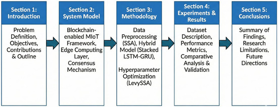
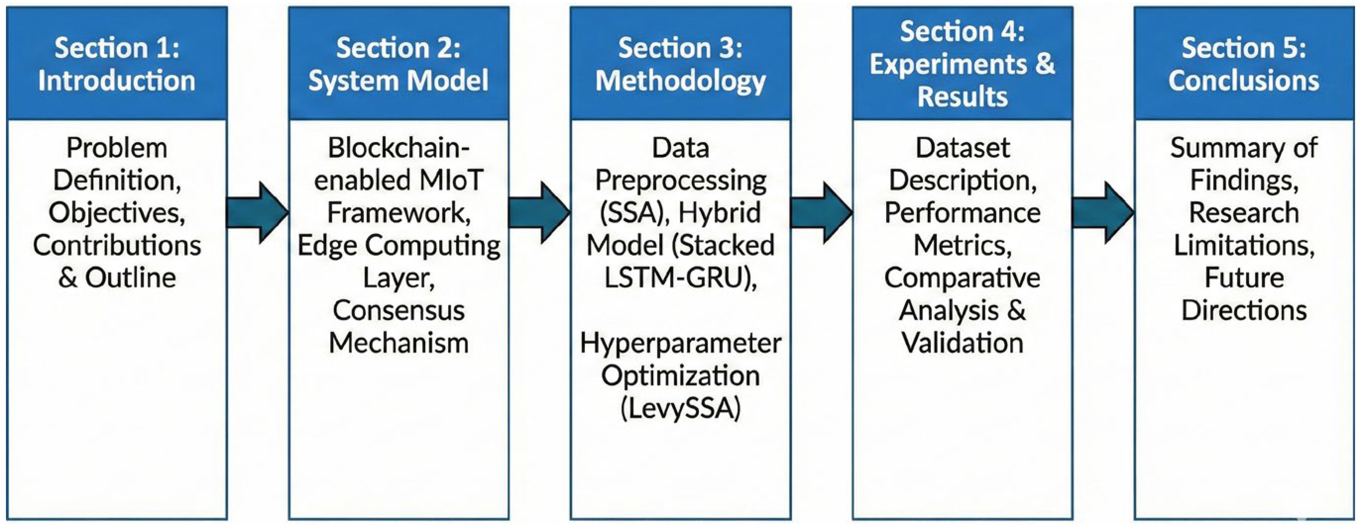
The remainder of the paper is organized as follows. Section 2 introduces the background of blockchain and classical GRU-RNN. Section 3 presents the proposed method in detail. In Section 4, the experimental study including the predictions of PV power generation and electricity load is given. The conclusions and possible future work are given in Section 5, as shown in Figure 1.
Figure 1.
Schematic organization of the paper showing the flow of the study.
2. Background
2.1. Introduction to Blockchain
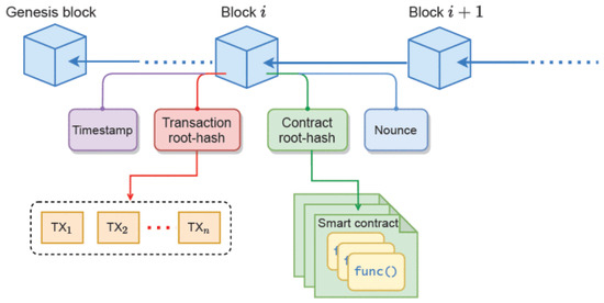
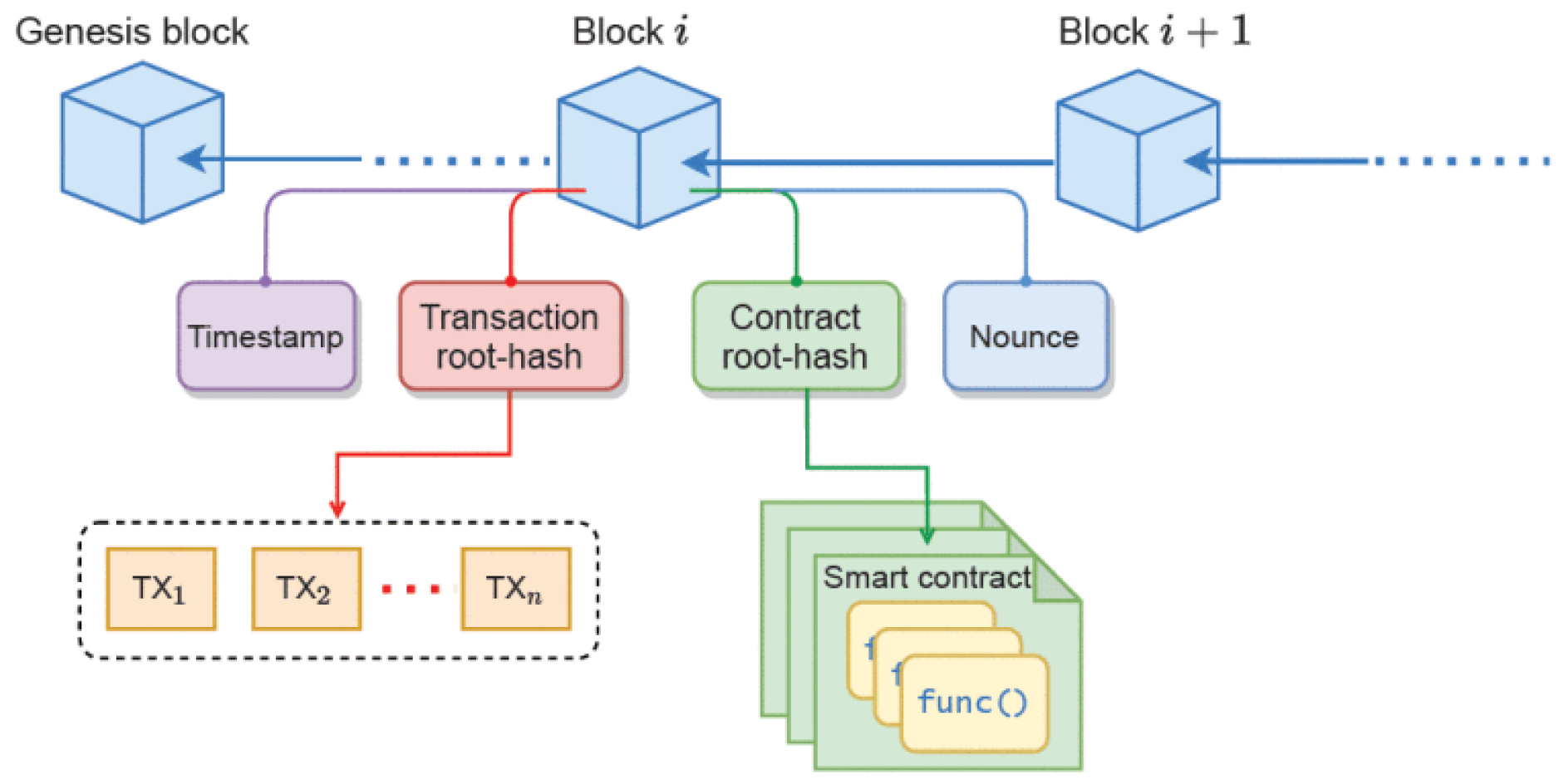
Blockchain originated from bitcoin, which is a cryptocurrency created by an unknown person or organization using the pseudonym Nakamoto in 2008 [23]. Blockchain is a growing chain of data packages (called blocks). The structure of a blockchain with several blocks is shown in Figure 2 [24]. The first block is called genesis block. The following block is then connected to its previous one through the hash value of the previous block. For example, block i + 1 in Figure 1 stores the hash value of block i. Each block also contains a timestamp and a nonce (a random number used for verifying the hash, root hash of all the transactions, and root hash of all the contracts) [25].
Figure 2.
Blockchain consisting of a number of blocks [24].
By its design, a blockchain has the characteristics of decentralization, integrity, and auditability [26]. Blockchains enable decentralized validation of transactions across the geographically distributed nodes so that a centralized authority of high cost and limited capacity can be avoided. With the cryptographic mechanisms (like asymmetric encryption algorithms, digital signature, and hash functions), the integrity of data packages in the blockchains can be guaranteed.
Blockchains also enable smart contracts that can automate the execution of contractual terms and clauses. The agreed contractual clauses are converted into executable computer programs and executed when certain conditions are met. The executions of the contracts is recorded in blockchains which are immutable due to the immutability of blockchains. Smart contracts guarantee appropriate access control and contract enforcement. Smart contracts can significantly simplify the administration procedure with increased efficiency and reduced risks, which is ideal for distributed IoT systems [27].
2.2. Introduction to LSTM
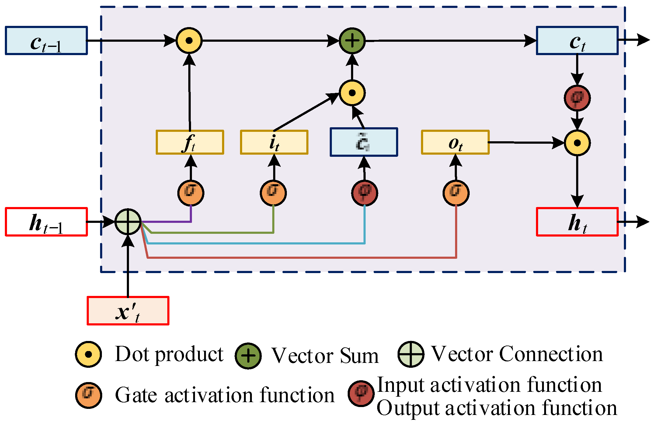
RNN has self-feedback connected neurons, which is more sensitive to time-series data. RNN has stronger forecasting performance compared with other deep learning models such as CNN, deep belief network (DBN), and stacked autoencoder (SAE). To address the gradient vanishing problem of RUU, LSTM has been developed by introducing a gating mechanism to improve the RNN for controlling the rate of accumulating information. The model structure of a classical LSTM is shown in Figure 3.
Figure 3.
The model structure of a classical LSTM.
The LSTM units are utilized to replace the traditional hidden neurons, formed by three gates called input gate (it), forget gate (ft) and output gate (ot), respectively [28]. The forget gate is used to control information that needs to be forgotten from the memory cell in the previous internal states (ct−1). The purpose of the input gate is to determine how much information needs to be preserved based on the memory cell in the current candidate state (). The output gate is applied to decide how much information needs to be output to the memory cell in the current external state (ct). For time-series data xt = {x1, x2, …, xt}, the calculation of LSTM can be expressed as follows:
where xt represents the input data at time t; ht represents the hidden state at time t; ht− 1 represents the hidden state at the previous time t − 1; σ (·) denotes the activation functions of the two gates; φ (·) denotes the activation functions of the input layers and output layers; is the dot product; Wxi, Wxf, Wxo and Wxc represent the weights connecting the input layer and the input gate, forget gate, output gate, and current candidate state, respectively; Uhz, Uhr, Uhc and Uxc denote the self-connection weights between the current time t and the previous time t − 1; bi, bf, boand bc are the biases of the input gate, forget gate, output gate and current candidate state in the LSTM.
3. The Proposed Method
3.1. Overall Framework
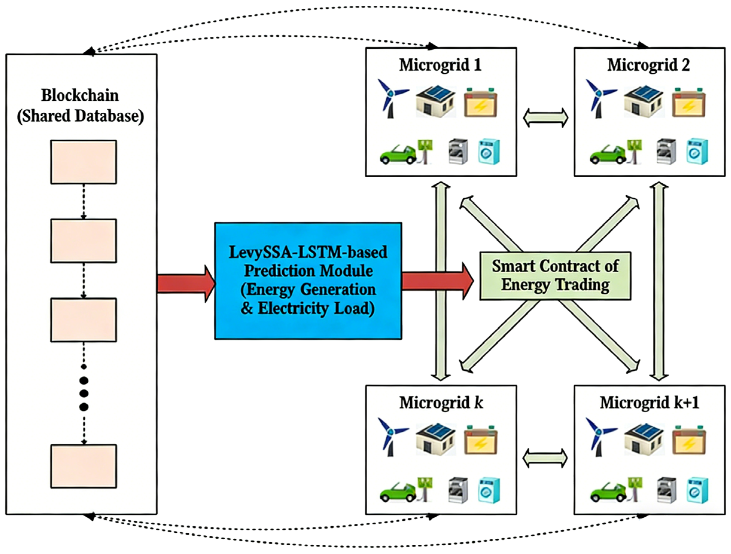
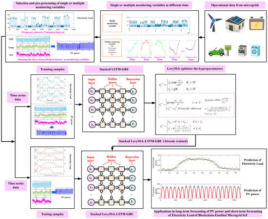
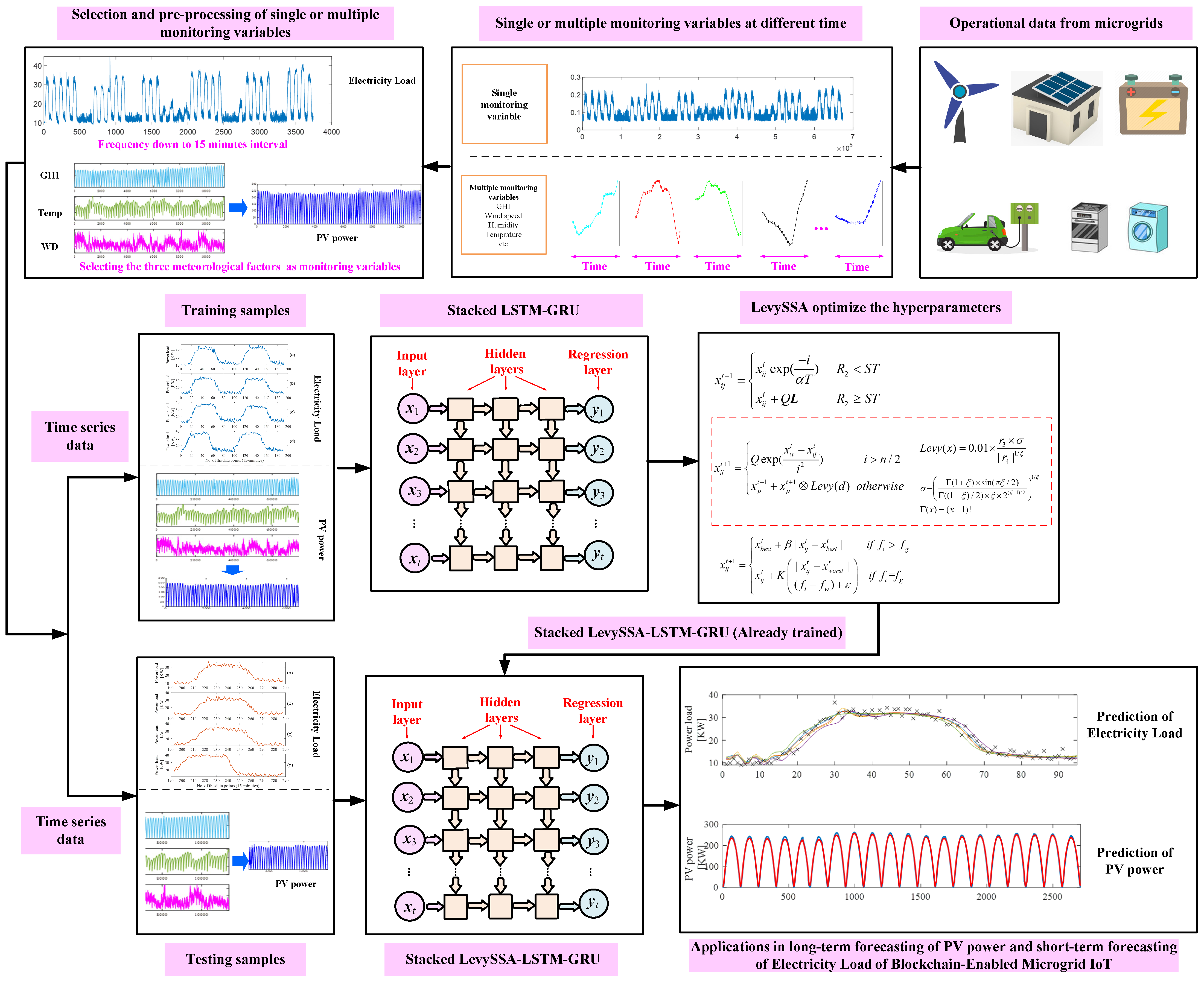
The overall framework of the proposed blockchain-enabled microgrid IoT is shown in Figure 4. The operational data of the microgrids from connected energy sources (PV, wind turbine, batteries, etc.), electricity consumers (EV charging, smart devices, etc.), and local weather condition sensors are packed and stored on the blockchain-based shared database with high security. Beyond ensuring privacy and security, the blockchain layer exerts a direct influence on the forecasting performance by guaranteeing the integrity of the training data. In unprotected MIoT networks, the predictive model is susceptible to ‘data poisoning’ attacks where compromised nodes inject false energy readings to skew the learning process. The integrated blockchain framework mitigates this risk through its consensus protocol, which validates the consistency of incoming data streams and rejects unverified or malicious transactions before they enter the database. This mechanism ensures that the LevySSA-LSTM-GRU model operates solely on high-quality, tamper-proof data, thereby preventing the statistical divergence and accuracy degradation that typically result from corrupted input datasets. To ensure the system meets the real-time and security demands of the microgrid environment, the underlying blockchain operates as a permissioned network, employing the Practical Byzantine Fault Tolerance (PBFT) consensus protocol. Unlike energy-intensive proof-of-work mechanisms, PBFT provides instant transaction finality with a latency of approximately 1–2 s, which is critical for timely energy trading and load balancing. Regarding cryptographic security, the framework utilizes SHA-256 for block integrity verification and the elliptic curve digital signature algorithm (ECDSA) (secp256k1 curve) for authenticating transaction origins. ECDSA is selected over RSA due to its smaller key size and lower computational overhead, making it ideal for resource-constrained MIoT sensors. In terms of storage and throughput specifications, the block size is capped at 1 MB with a target block generation interval of 10 s. This configuration supports a transaction throughput capable of handling the synchronized 5 min data reporting intervals from the distributed nodes without inducing network congestion. To strictly address the scalability challenges associated with the quadratic communication complexity of the PBFT consensus mechanism as the number of MIoT nodes increases, the framework incorporates a hierarchical data processing strategy. Rather than broadcasting every raw sensor reading directly to the consensus layer, the system utilizes a ‘compute-off-chain, verify-on-chain’ architecture where high-frequency raw data processing and model inference occur locally at the edge nodes. Only the compact transaction hashes, prediction outcomes, and critical state updates undergo the consensus process and permanent storage. For scenarios requiring massive expansion beyond a single microgrid cluster, this architecture supports a sidechain topology where independent microgrids operate on parallel sidechains to handle local high-throughput transactions, anchoring only aggregated state roots to the main blockchain. This design effectively decouples the consensus latency from the total node count, ensuring that the system throughput remains stable even as the network scales. Through the LevySSA-LSTM-based prediction module, energy generation and electricity load for each microgrid can be accurately estimated using the highly reliable data from the blockchain. With accurate energy prediction, adaptive pricing of the electricity trade between microgrids can be achieved. Then, smart contracts can be executed without a central agency, which optimizes the energy management of the microgrids. This study has a specific focus on the accurate prediction of energy generation and electricity load, which is crucial to the overall efficiency of smart microgrids.
Figure 4.
The overall framework of the blockchain-enabled microgrid IoT.
3.2. Stacked LSTM-GRU
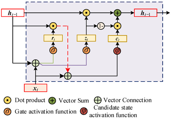
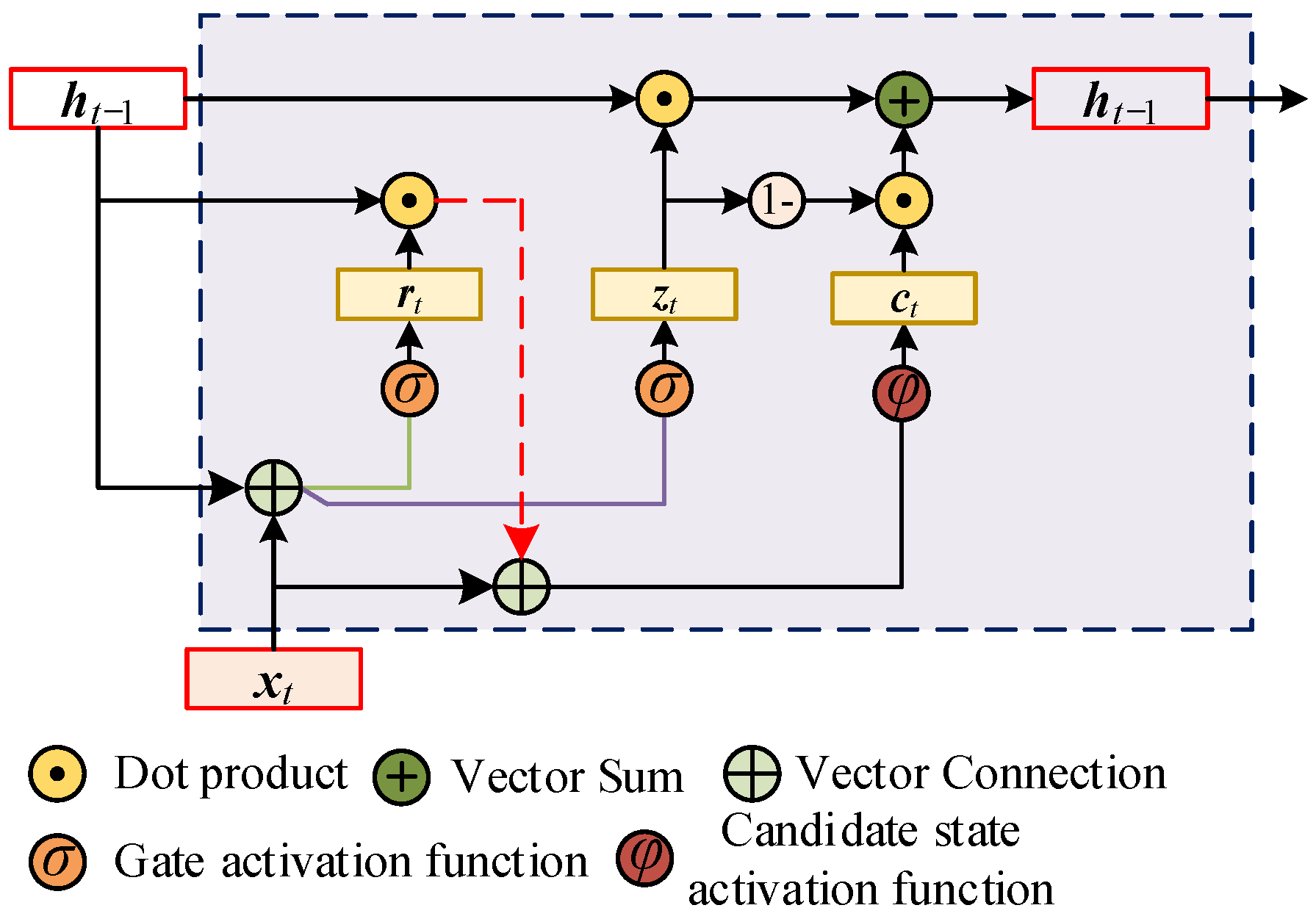
In this study, we adopt LSTM and GRU because microgrid forecasting is inherently a sequential learning task with non-stationary and long–short temporal dependencies. LSTM is effective in retaining long-term information through a memory cell mechanism, whereas GRU has a simpler gating structure with fewer parameters, enabling faster convergence and reduced overfitting. Stacking LSTM and GRU therefore captures multi-scale temporal patterns while remaining computationally efficient for MIoT nodes. Alternative models such as CNN-based predictors, tree ensembles (e.g., XGBoost/LightGBM), or transformer architectures may require larger datasets, heavier computational resources, or additional feature engineering, making them less practical in our edge-oriented MIoT deployment scenario. GRU-RNN has a simpler structure compared with LSTM, as shown in Figure 5. GRU controls the amount of information to be preserved and accepted by introducing update gates, rather than introducing additional memory units, which can reduce the calculation costs [29]. Unlike the LSTM, the GRU architecture simplifies the sequential modeling by merging the cell state and hidden state into a single unified state. The mathematical formulation of the GRU unit at time step t is governed by the following equations. First, the update gate zt and the reset gate rt are computed to control the information flow, computed as the following:
Figure 5.
The model structure of GRU-RNN.
Subsequently, the candidate hidden state ht utilizes the reset gate to ignore irrelevant past information, and the final hidden state ht is computed as a linear interpolation between the previous state and the candidate state:
where xt and ht denote the input vector and the output hidden state vector at time t, respectively, while ht − 1 represents the hidden state at the previous time step. The matrices Wz, Wr, Wh represent the feedforward weights connecting the input layer to the update gate, reset gate, and candidate state, whereas Uz, Ur, Uh denote the recurrent weight matrices, connecting the previous hidden state to the respective gates. The vectors bz, br, bh correspond to the bias terms for each component. The symbol σ (·) denotes the sigmoid activation function, tanh (·) denotes the hyperbolic tangent activation function, and the operator represents the element-wise multiplication (Hadamard product). This formulation ensures that the model can effectively capture long-term dependencies by dynamically adjusting the update and reset mechanisms.
Training LSTM with long sequences can improve its effectiveness, but takes significantly more time. Also, LSTM contains more parameters that make it difficult to train. To reduce training time and the number of model parameters, the GRU layers are introduced into LSTM. Therefore, the LSTM-GRU structure is proposed in this paper, and it is formulated as follows:
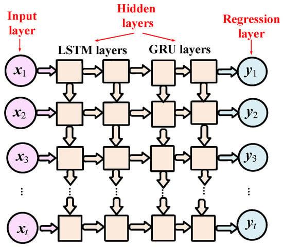
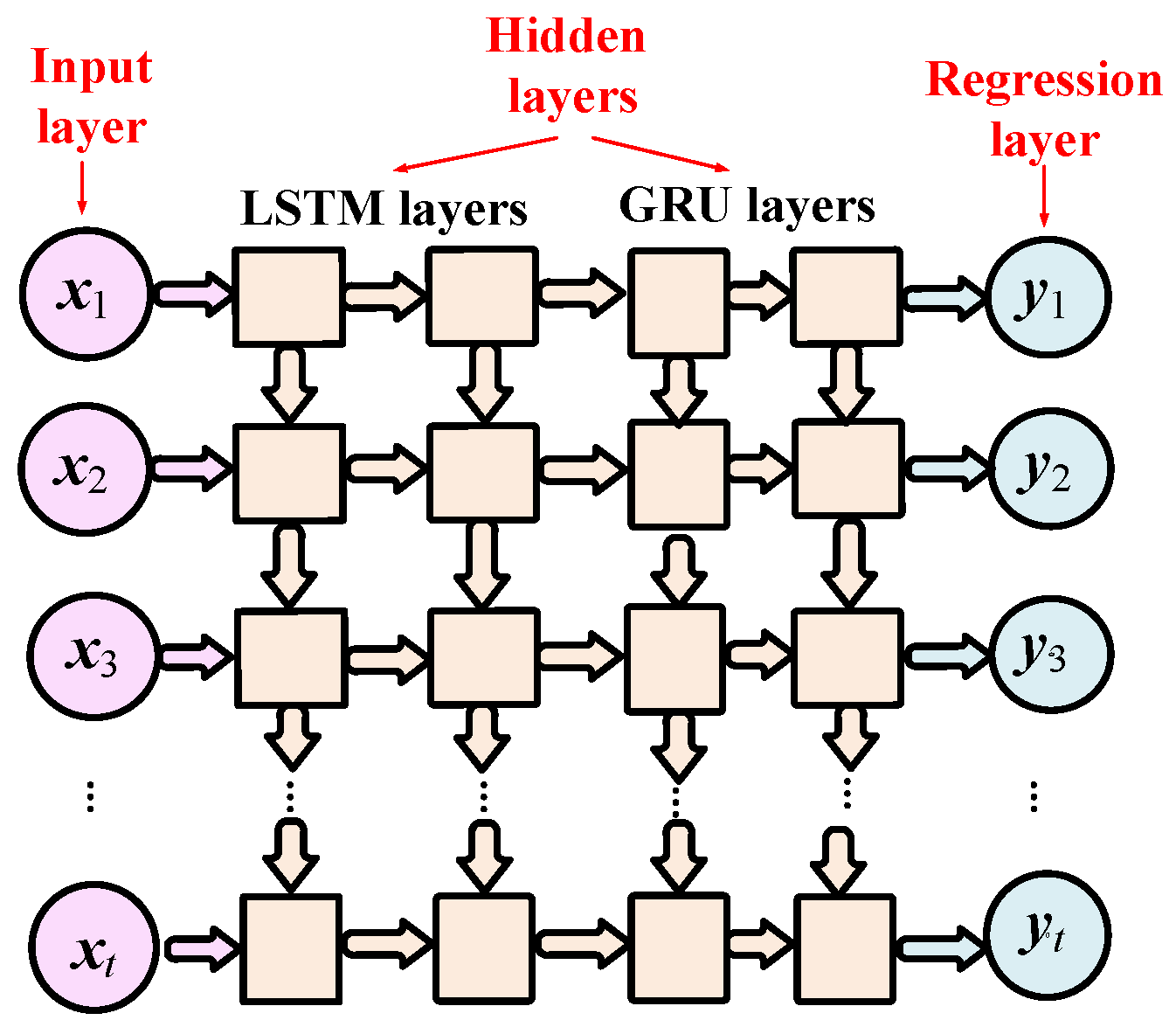
The time-series signals often exhibit highly non-linear and non-smooth characteristics between input and output. Therefore, a stacked LSTM-GRU is established by stacking multiple LSTM layers and GRU layers. As shown in Figure 6, a stacked LSTM-GRU is built for prediction by constructing a regression layer based on the input layer and hidden layers; it is defined as follows:
where is the prediction value after the regression layer; Uyh is the weight matrix of the regression layer; by is the bias vector of the regression layer; σ (•) is the activation function in the regression layer. The specific architecture of the stacked LSTM-GRU follows a tapered ‘funnel’ design. Theoretically, this structure serves a dual purpose: the wider initial layers capture diverse, high-frequency temporal dependencies from the raw MIoT data, while the subsequent narrower layers force the network to learn more compact, high-level abstractions. This dimensionality reduction acts as an implicit regularizer, mitigating the risk of overfitting while preserving essential long–short-term memory representations. To accommodate the diverse computational capabilities of MIoT nodes, such as low-power sensors and high-performance edge servers, we implement a scalable width multiplier α in (0, 1]. This parameter modulates the layer width to α times NL, allowing the system to balance prediction accuracy with latency and energy demands. This strategy ensures the predictor remains deployable across heterogeneous hardware without necessitating fundamental architectural modifications.
Figure 6.
Stacked LSTM-GRU for prediction using time-series data.
3.3. Sparrow Search Algorithm Optimized by Levy Flights
To improve the forecasting performance of the proposed model, the sparrow search algorithm (SSA) optimized by Levy flights (LevySSA) is established to optimize the hyperparameters of the stacked LSTM-GRU. To strictly adhere to mathematical programming principles, we formulate this hyperparameter tuning as a constrained non-linear optimization problem. We define the decision variable vector x = [x1, x2, x3]T, corresponding to the initial learning rate, the gradient clipping threshold, and the training iterations, respectively. The objective function F (x) represents the mean squared error (MSE) evaluated on the validation set, serving as the quantitative metric for model fidelity. Consequently, the optimization model is explicitly stated as follows: Minimize F (x) subject to the box constraints L ≤ x ≤ U, where L and U denote the strictly defined lower- and upper-bound vectors of the search space. The LevySSA algorithm described below is then applied to solve this global optimization problem by efficiently exploring the defined feasible region. SSA is a new type of swarm intelligence optimization algorithm, which can simulate the foraging process of sparrow to obtain the solution of the optimization problem [30]. Compared with SSA, levySSA can speed up convergence and improve the capability of searching for globally optimal solutions by introducing the Levy flight algorithm [19].
Assuming that there are n sparrows in the d-dimensional searched space, the position of the ith sparrow in the d-dimensional searched space is Xi= [xi1, xi2, …, xid], where i = 1, 2, …, n, j = 1, 2, …, d; xij is the position of the ith sparrow in the jth dimensional. The proportion of producers in the general population is 10–20%, and the location updating the formula is as follows:
where t is the current number of iterations, T is the maximum number of iterations, is the value of ith sparrow in the jth dimension, is the random number, Q is the random number that submits the standard normal distribution, and are the precaution value and security threshold, and L is a matrix (1 × d) with all ones.
Except for the producers, the rest of the sparrows are regarded as the scroungers. To avoid the algorithm falling into local optimum, Levy flight is introduced into the formula of the scroungers’ location update to improve the global searching ability, and the improved formula is described as follows:
where is the best location of producers. The mechanism of Levy flight is as follows:
where r3 and r4 are random numbers within the range [0, 1]; ξ = 1.5. σ is calculated as follows:
Assume that the sparrows, which are aware of the danger or threat from predators, account for 10–20%. The initial locations of these sparrows are stochastically generated in the population. Therefore, the expression of the global optimal location is constructed as follows:
where xbest is the current global optimal location, and β is step size control parameter that obeys the standard normal distribution of random numbers. is a random number. fi is the fitness value of the current sparrow. fg and fw are the current global optimization and worst fitness value separately. ε is the minimal constant which can avoid the divisor equal to zero. To facilitate reproducibility and clarify the computational logic, the overall execution procedure of the LevySSA is formalized in Algorithm 1. The process begins by initializing the population within the specified hyperparameter boundaries and defining the algorithm parameters. In each iteration loop, the algorithm first evaluates the fitness (MSE) of all individuals and ranks them to identify the current global optimum. The population is then divided into producers and scroungers. Producers, responsible for global exploration, update their positions according to Equation (11). Crucially, to mitigate the risk of stagnation in local optima, the scroungers incorporate the Levy flight mechanism into their position updates as defined in Equation (12), which introduces heavy-tailed random jumps to expand the search scope. Subsequently, a random subset of sparrows sensing predation risk updates their positions via Equation (15). Finally, the algorithm enforces boundary constraints to ensure all hyperparameters remain within the feasible region before proceeding to the next generation. This iterative process continues until the maximum number of iterations is reached, yielding the optimal hyperparameter set xbest, as illustrated in Algorithm 1.
| Algorithm 1. Pseudocode of the LevySSA for hyperparameter optimization |
| Input: Maximum iterations T; Population size N; Lower and upper bounds L, U; Safety threshold ST. Output: Optimal hyperparameters xbest. 1: Initialize population set X randomly within L, U and define parameters. 2: While t < T do 3: Calculate fitness fi for all sparrows using the validation MSE. 4: Sort the population and identify the current best individual xbest. 5: For each sparrow i = 1 to N do 6: If i ≤ Number of Producers then 7: Update producer position using Equation (11). 8: Else (Scroungers) 9: Update scrounger position xit + 1 utilizing Levy flight mechanism via Equation (12). 10: End If 11: End For 12: Randomly select sparrows (aware of danger) and update positions using Equation (15). 13: Check and enforce boundary constraints: xi = max(L, min(U, xi)). 14: t ← t + 1. 15: End While 16: Return xbest |
Distinct from existing hybrid models that utilize standard metaheuristics like PSO or genetic algorithms, the proposed approach fundamentally addresses the ‘accuracy–efficiency’ dilemma inherent in edge-based microgrid forecasting. While traditional algorithms often succumb to premature convergence in high-dimensional hyperparameter spaces, the integrated LevySSA mechanism utilizes heavy-tailed step distributions to actively escape local optima, ensuring robust convergence with fewer iterations. This is coupled with a custom ‘funnel-structured’ stacked LSTM-GRU architecture, which strategically reduces dimensionality to minimize computational overhead. This method provides a system-level optimization tailored for resource-constrained MIoT nodes, rather than merely stacking layers for marginal accuracy gains.
3.4. Implementation of the Proposed Energy Prediction Method
This paper develops a blockchain-based approach for predicting energy generation and electricity load in the smart microgrid. To bridge the off-chain predictive intelligence with on-chain execution, the system employs an automated interaction protocol. The trained LevySSA-LSTM-GRU model resides on the local edge server of the microgrid controller to minimize inference latency. Upon generating a forecast for the upcoming 15 min interval, the edge node automatically constructs a transaction containing the predicted values and digitally signs it using its private key. This transaction broadcasts to the blockchain network via a Web3 interface, serving as a trusted oracle feed that triggers the ‘EnergyTrading’ smart contract function. Regarding temporal feasibility, the total system latency comprises the model inference time (approximately 150 milliseconds), network propagation, and the PBFT consensus delay (1–2 s as defined in Section 3.1). Consequently, the cumulative latency from prediction output to confirmed contract execution remains below 5 s. Given that the energy management system operates on a 15 min dispatch cycle, this negligible delay ensures that the smart contracts utilize fresh, valid data for real-time pricing and load balancing decisions without compromising system stability. The implementation of the energy prediction method is shown in Figure 7. The procedure is as follows.
Figure 7.
The overall framework of the proposed energy prediction method.
Step 1: Request the operational data of the microgrids from the blockchain-based shared database including the historical data of energy generation, electricity load, and weather conditions.
Step 2: Divide the samples into training and testing datasets.
Step 3: Build a stacked LSTM-GRU with optimal hyperparameters using LevySSA. The MSE of the stacked LSTM-GRU is used as the fitness function of the LevySSA algorithm by optimizing the initial learning rate, the gradient threshold, and the number of iterations.
Step 4: Train the stacked LSTM-GRU model with the training dataset to establish an accurate mapping relationship between the monitoring variables and the output variables.
Step 5: Validate the forecasting effectiveness of the stacked LevySSA-LSTM-GRU model using the testing samples.
Step 6: Implement the model and make predictions in the operational microgrids.
4. Experimental Evaluation
To assess the performance of the proposed method in forecasting renewable energy generation and electricity load, two experiments are implemented: PV power prediction using multiple meteorological parameters and electricity load prediction using historical load data.
4.1. Experiment One: PV Power Forecasting
4.1.1. Data Description and Experimental Setup
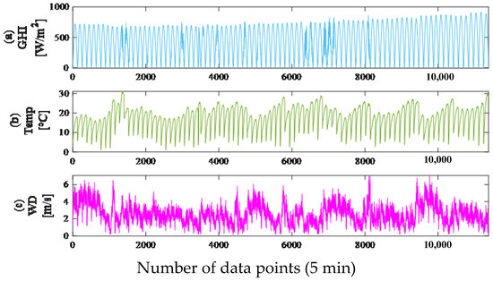
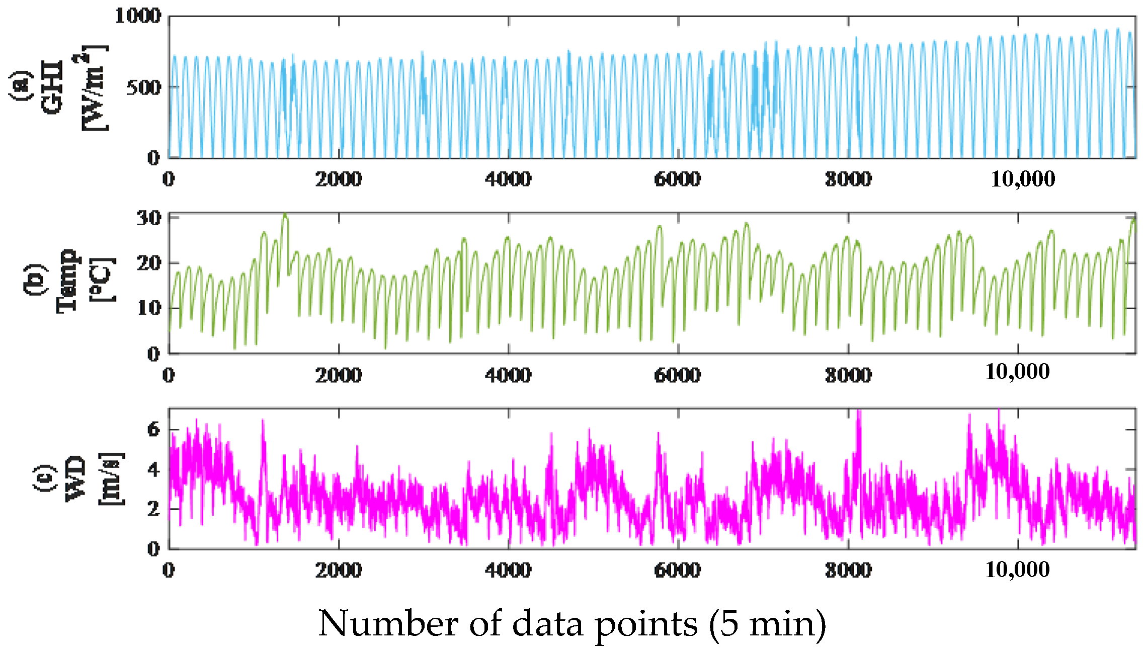
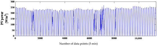
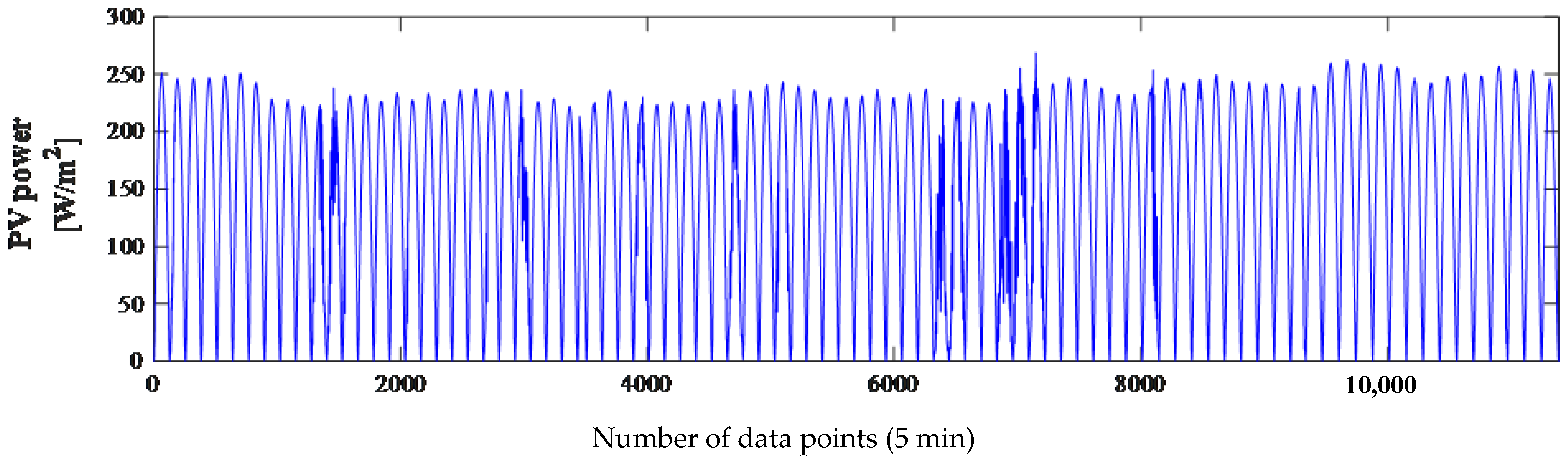
In this experiment, the dataset contained the actual PV power generation every 5 min from June to August 2019 together with meteorological conditions every 5 min at Yulara in the south of the Northern Territory of Australia [25]. The meteorological data includes global horizontal irradiance (GHI), temperature (Temp), and wind speed (WD). These variables are correlated to PV power and are used as input variables, as shown in Table 1. The three input variables and one output variable have significant non-linear and non-stationary characteristics, as shown in Figure 8 and Figure 9. The variables contain 11,385 data points of the time series, marked as , , and , respectively. Prior to model training, the raw dataset underwent rigorous preprocessing to ensure data quality and temporal alignment. First, addressing the sampling rate mismatch highlighted by the interval difference between the meteorological conditions (collected every 5 min) and the PV power generation (recorded every 15 min), we aligned the datasets by resampling the meteorological data. Specifically, we calculated the mean value of the three 5 min meteorological readings (GHI, temperature, and wind speed) corresponding to each 15 min window to strictly match the timestamps of the PV power output. Second, to handle missing values caused by sensor errors or transmission delays, we applied linear interpolation for gaps shorter than one hour, while days with extensive missing data were excluded from the dataset to maintain continuity. Third, regarding outlier filtering, we employed a statistical approach where data points deviating by more than three standard deviations from the moving average were flagged as anomalies and replaced with the interpolated values of their neighbors. Following these cleaning and alignment steps, the synchronized data were then normalized using the Z-score method as described in the subsequent equation, ensuring the input features were robust and scale-consistent for the deep learning model.
Table 1.
Descriptions of the input and output variables.
Figure 8.
The three input variables: (a) GHI; (b) temp; (c) WD.
Figure 9.
The output variable from June to Aug 2019.
The predictive model is to establish a non-linear mapping relationship between the input and output variables, denoted as . The data are first normalized to the scale of [0, 1] using the z-score method for model training and forecasting, which transforms the features to have a mean of zero and a standard deviation of one. The transformation is defined as x’ = (x − μ)/σ, where x is the original value, μ represents the mean, and σ represents the standard deviation of the feature. To avoid data leakage, μ and σ are computed strictly from the training set and subsequently applied to normalize the test set. To assess the performance of the proposed method in forecasting renewable energy generation and electricity load, two experiments were implemented: PV power prediction using multiple meteorological parameters and electricity load prediction using historical load data.
Regarding the optimization objective within the experimental setup, we strictly utilized the MSE as the sole fitness function for the LevySSA algorithm. We selected MSE specifically because it imposes a quadratic penalty on large deviations, which aligns with the microgrid’s operational requirement to strictly minimize extreme prediction errors that jeopardize grid stability. Furthermore, the smooth gradient of the MSE function ensures more stable convergence for the LevySSA compared to non-differentiable or constant-gradient alternatives like mean absolute error (MAE). Consequently, the algorithm optimizes the initial learning rate, the gradient threshold, and the number of iterations to minimize this quadratic objective, while we comprehensively evaluated the final model robustness using multiple metrics including MAE, root mean square error (RMSE), and correlation coefficients (R2) to ensure generalized performance. Three indices were used to evaluate the prediction effectiveness, including RMSE, MAE and R2:
where is the actual PV power output value, is its forecasting value, and n represents the total number of the testing samples. To strictly prevent data leakage and preserve temporal continuity, the dataset is partitioned chronologically rather than via random shuffling. The first 8676 samples (approximately 76% of the total dataset) constitute the training set, which allows the model to learn the temporal dependencies and daily periodicities inherent in the early phase of the observation period. The subsequent 2709 samples (the remaining 24%) serve as the test set. This strict temporal separation ensures that the model is evaluated solely on future unseen data, thereby reflecting a realistic forecasting scenario where historical data predicts future outcomes.
In addition to the standard point forecasting metrics, we employ two specific metrics to evaluate the quality of the constructed prediction intervals (PIs). The first is the prediction interval coverage probability (PICP), which measures the reliability of the PIs by calculating the percentage of actual target values that fall within the predicted lower and upper bounds. It is mathematically defined as follows:
A PICP value close to the nominal confidence level (e.g., 95%) indicates high reliability. The second metric is the mean prediction interval width (MPIW), which assesses the sharpness of the PIs. A narrower interval indicates lower uncertainty and higher precision, provided that the coverage probability is satisfied. The MPIW is calculated as follows:
Ideally, a robust forecasting model minimizes MPIW while maintaining a PICP higher than the nominal confidence level.
To ensure experimental reproducibility and quantify computational overhead, all algorithms operate within the TensorFlow 2.6 deep learning framework using Python 3.9. The hardware environment consists of a high-performance workstation equipped with an Intel Core i9-12900K CPU @ 3.20 GHz, 64 GB of RAM, and an NVIDIA GeForce RTX 3090 GPU. Under this configuration, the average training time for the proposed LevySSA-LSTM-GRU model stabilizes at approximately 150 s. This duration reflects the convergence efficiency of the LevySSA optimization, which rapidly locates the optimal hyperparameter set without necessitating exhaustive computational resources.
4.1.2. Comparison with Other Methods
To validate the superiority of the proposed method in PV power forecasting, a comparison with six types of stacked RNNs and two classical machine learning models is carried out. For the stacked LSTM-GRU, the input and output layer sizes depend on the number of the input and output variables that are three and one, respectively. The hyperparameters of the LSTM-GRU are determined by the LevySSA optimization algorithm, where the initial learning rate, gradient threshold, and number of iterations are searched in the ranges [0.003, 0.005], [0.8, 1], and [100, 250], respectively. The optimal values of the three hyperparameters were 0.005, 0.9471, and 150, respectively. The number of hidden layers NH and neurons in every hidden layer NL was decided by grid search, where NH ∈ {2, 3, 4, 5} and NL ∈ {50, 100, 150, 200}. The number of neurons and layers in the input layer, LSTM hidden layers, GRU hidden layers, and output layers are “3-200-100-1” and “1-2-2-1”, respectively. While grid search is used to identify the candidate hyperparameters, we further conduct a sensitivity analysis to theoretically justify the selection of depth NH and width NL regarding the trade-off between performance and model complexity. As shown in Table 2, increasing the depth from two to three yields a significant reduction in nRMSE. However, extending NH to four or five results in diminishing returns (less than 0.5% improvement in accuracy) while drastically increasing the parameter count and training time. Thus, the configuration of NH = 3 is selected as the optimal balance point for MIoT edge deployment.
Table 2.
Sensitivity analysis of architecture depth and width.
While the LevySSA algorithm is dedicated to optimizing the learning dynamics (specifically learning rate, gradient threshold, and iterations), other influential structural hyperparameters are pre-determined to maintain a manageable search space without compromising performance. The sequence window size (Twin) is established using partial autocorrelation function (PACF) analysis rather than stochastic search. The analysis reveals significant temporal dependencies up to lag seven, which aligns with the daily and weekly operational cycles of the microgrid; thus, the regression step is fixed at seven to physically capture these patterns. Furthermore, the batch size and dropout rate are selected based on preliminary convergence tests. To empirically validate these fixed choices, we conduct a supplementary sensitivity analysis summarizing the impact of varying batch sizes and window lengths on model nRMSE and training time. As presented in Table 3, increasing the window size from seven to fourteen yields only a marginal improvement in nRMSE (approximately 0.0006 reduction) but increases the computational cost by over 40%. Similarly, a batch size of 64 provides the optimal balance between gradient stability and convergence speed compared to sizes of 32 or 128. These results confirm that fixing these structural parameters allows the LevySSA to focus its computational resources efficiently on optimizing the critical convergence hyperparameters.
Table 3.
Sensitivity analysis of fixed hyperparameters.
The hyperparameters of the other methods are determined as follows. The stacked SSA-LSTM-GRU and PSO-LSTM-GRU have the same number of neurons and hidden layers as the stacked LSTM-GRU. The SSA and PSO algorithms have the same range for searching optimized hyperparameters as the LevySSA algorithm. Their hyperparameters are set as “169, 0.031, 0.9929” and “148, 0.045, 0.9397”, respectively. To rigorously validate the computational efficiency, we perform a comparative complexity analysis of LevySSA against standard SSA and PSO. Theoretically, all three stochastic optimization algorithms share a time complexity of O (I·P·D) and a space complexity of O (P·D), where I denotes the iteration count, P is the population size, and D represents the hyperparameter dimensionality. While the Levy flight mechanism introduces a marginal floating-point overhead per step, it fundamentally alters the search dynamics by enabling long-range jumps to escape local optima. Empirically, this enhanced global search capability allows LevySSA to converge within approximately 150 iterations, whereas standard SSA and PSO typically require over 200 to 250 iterations to reach comparable loss levels. Consequently, the decrease in required convergence iterations outweighs the slight per-iteration cost, yielding an overall reduction of approximately 15–20% in total training time compared to the baselines, which substantiates the method’s contribution to minimizing training costs in resource-constrained MIoT environments. The number of neurons and layers in input, hidden, and output layer for stacked LSTM, stacked GRU, and stacked BiLSTM is “3-200-1”, and “1-2-1”, respectively. And they have the same hyperparameter values as the stacked LSTM-GRU. The initial learning rate, gradient threshold, and the number of iterations of these models are 0.005, 1, 250. The KELM model uses a radial basis function kernel and a sigmoid function for the activation function of the hidden layer. And its kernel parameters, regularization parameters, and the number of neurons are set to six, four, and twenty, respectively. The training functions for the NARX network model are “trainlm”, and input delay, feedback delay, and the hidden layer size are set to 5,10, and 100, respectively. The random forest (RF) model employs the Gini impurity criterion for measuring the quality of a split. And its number of decision trees (estimators), the maximum depth of each tree, and the minimum number of samples required to split an internal node are set to 100, 20, and 5, respectively. The multilayer perceptron (MLP) model utilizes the rectified linear unit (ReLU) as the activation function for the hidden layers and the ‘adam’ solver for weight optimization. And its hidden layer structure (neurons per layer), initial learning rate, and maximum number of iterations are defined as (100, 50), 0.001, and 500, respectively.
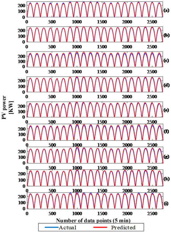
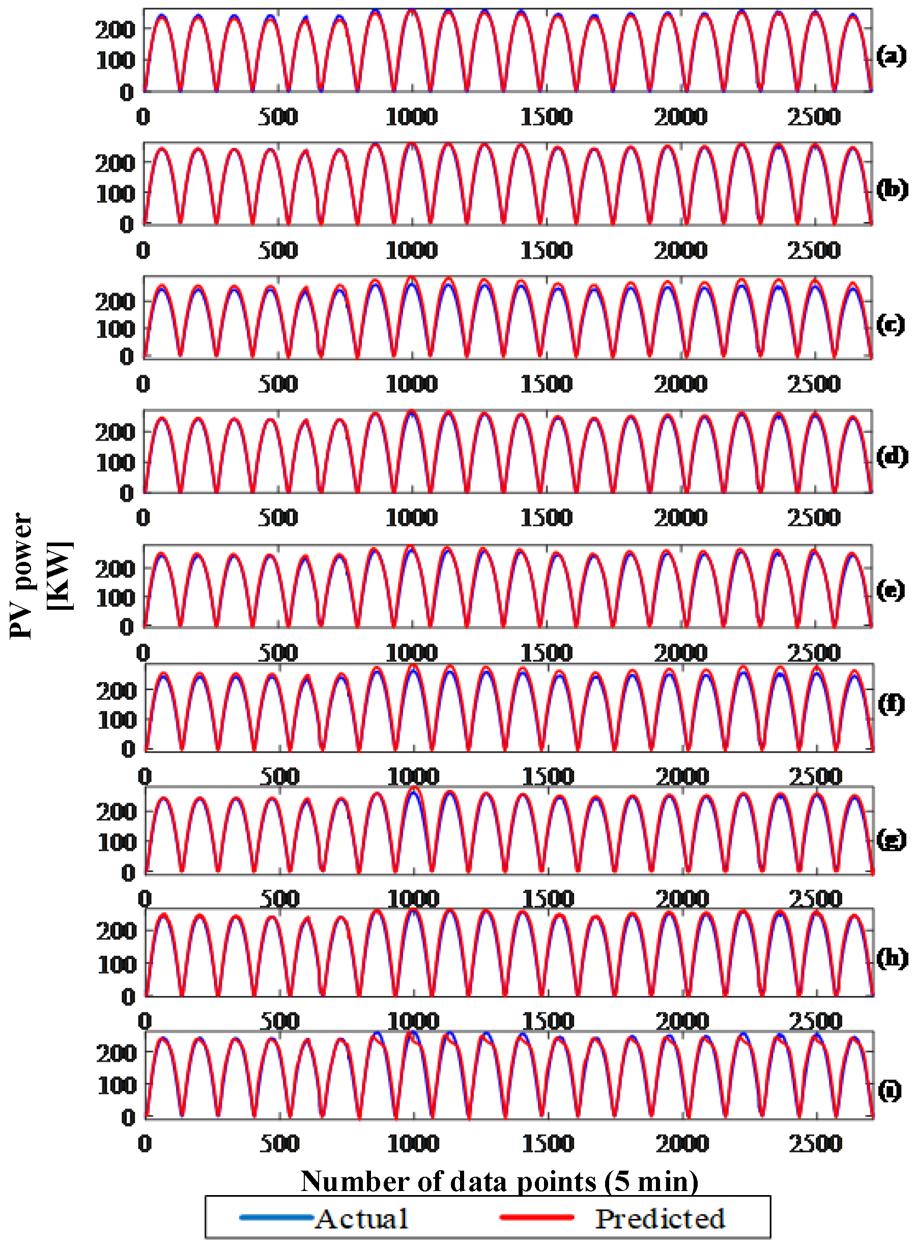
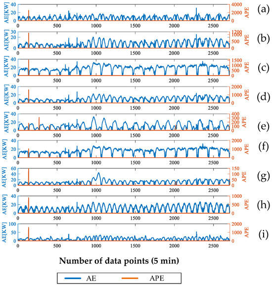
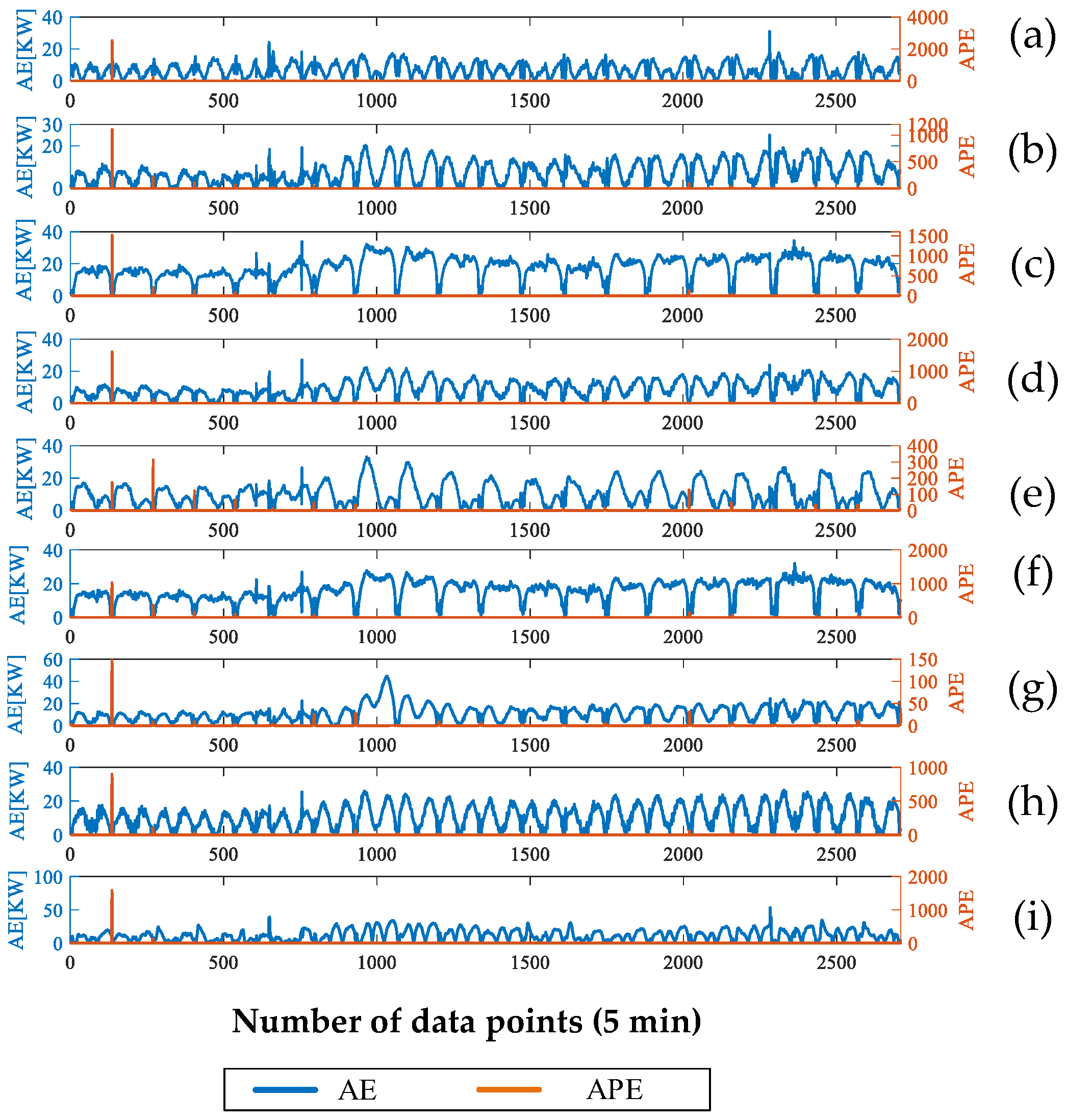
The forecasting results using the different methods are shown in Figure 9 and Figure 10, which show the absolute errors (AEs) and absolute percentage errors (APEs) for the different methods. Figure 9 and Figure 10 display the forecasting results and error metrics with standardized axes for clarity. In both figures, the horizontal axis represents the ‘time step (5 min intervals)’, aligning with the temporal resolution of the dataset. For Figure 9, the vertical axis indicates the ‘power (kW)’, allowing for a direct comparison of the amplitude between actual and predicted values. In Figure 10, the left vertical axis denotes the ‘absolute error (kW)’, while the right vertical axis represents the ‘absolute percentage error (%)’. This uniform labeling confirms that the proposed method consistently maintains low error magnitudes across the test horizon. It can be seen that the proposed method gives the smallest range of absolute error values (ranging in [0, 32]), compared with the machine learning methods. From Table 4, the numbers of errors between forecasting and actual data (normalized form) within ±0.02, ±0.05, and ±0.1 are 628, 1427, and 2281, respectively, which are more than several other methods. To rigorously verify the assumption of error normality beyond visual inspection, we apply the Kolmogorov–Smirnov test to the prediction residuals. The obtained test statistic (D = 0.024) with a corresponding p-value of $0.15$ indicates that the null hypothesis of a normal distribution is not rejected at the 5% significance level. This statistical validation confirms that the model’s errors follow a Gaussian distribution centered around zero, which implies that the proposed LevySSA-LSTM-GRU model effectively captures the underlying data trends without introducing systematic bias.
Figure 10.
Forecasting results of nine trials: (a) Method 1; (b) Method 2; (c) Method 3; (d) Method 4; (e) Method 5; (f) Method 6; (g) Method 7; (h) Method 8; (i) Method 9.
Table 4.
Statistical error (normalized form) information in Experiment 1.
Table 5 lists the three evaluation indices for the different methods. According to Table 3, the nRMSE, nMAE, and R2 of the proposed method are 0.0535, 0.0455, and 0.9898, respectively. Compared with other methods, the proposed method achieves the least nRMSE for PV power prediction using multiple meteorological factors. It demonstrates that the proposed stacked LevySSA-LSTM-GRU method has superiority in time-series modeling.
Table 5.
Evaluation indices in Experiment 1.
To further assess robustness, we report the cumulative error distribution over the PV test set. The proposed LevySSA-LSTM-GRU yields 23.18%, 52.68%, and 84.20% of predictions with absolute normalized errors within ±0.02, ±0.05, and ±0.10, respectively. In comparison, SSA-LSTM-GRU reaches 20.45%, 43.82%, and 78.44% under the same thresholds, confirming that the proposed method produces more concentrated errors and improved stability. To rigorously validate the robustness of the forecasting performance, we extend the evaluation to include uncertainty quantification (UQ) across all nine comparative models. Building upon the statistical validation of error normality, we construct 95% prediction intervals (PIs) for each method. Table 5 presents the uncertainty quantification metrics, listing the MPIW and PICP for the proposed method alongside the eight baselines. The results reveal a distinct performance hierarchy. The proposed LevySSA-LSTM-GRU (Method 1) demonstrates superior performance, achieving the highest PICP of 0.9285 while maintaining the narrowest interval width of 0.58. The other hybrid optimized models (Methods 2 and 3) follow, showing improved reliability over the standalone deep learning models (Methods 4–7). Notably, the traditional shallow models, KELM (Method 8), NARXN (Method 9), RF (Method 9), and MLP (Method 9) exhibit the widest uncertainty bands and lowest coverage probabilities (below 72%), indicating their limited capacity to capture the high-volatility dynamics of PV generation. This comprehensive analysis confirms that the proposed LevySSA optimization strategy not only minimizes point prediction error but also significantly reduces probabilistic uncertainty, aligning with the stringent reliability requirements for renewable energy trading [31].
4.2. Experiment Two: Power Load Forecasting
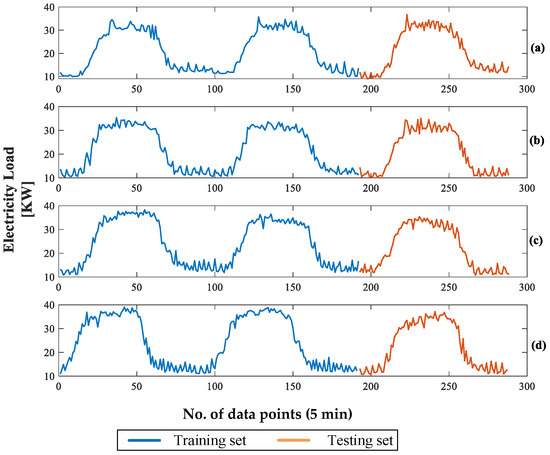
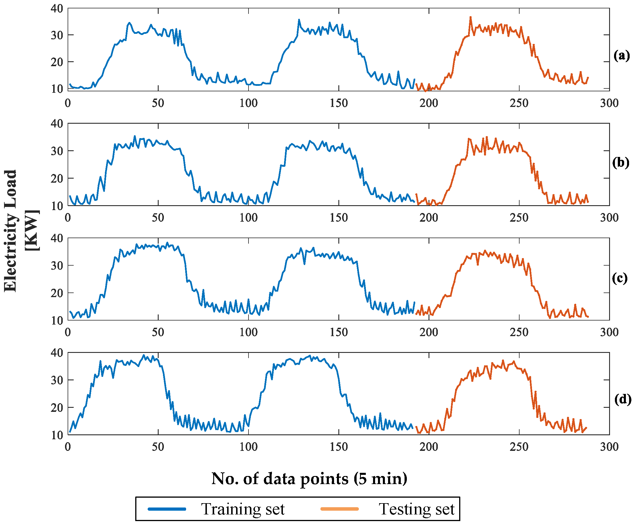
In this experiment, the proposed stacked LevySSA-LSTM-GRU is applied for short-term forecasting of the electricity load. A dataset containing household electricity load of every 5 min from 13 May 2019 to 17 June 2019 in Belgium is used [32]. To check the robustness of the forecasting method, four randomly selected intervals of three-day data are selected. In each sample, the first two days (96 × 2 = 192 data points) are used as the training set, and the third day (96 data points) is used as the test set. The four samples (1) from 13 May to 15 May, (2) from 29 May to 31 May, (3) from 4 June to 6 June, and (4) from 13 June to 16 June, are plotted in Figure 11.
Figure 11.
AE and APE of the forecasting of nine trials: (a) Method 1; (b) Method 2; (c) Method 3; (d) Method 4; (e) Method 5; (f) Method 6; (g) Method 7; (h) Method 8; (i) Method 9.
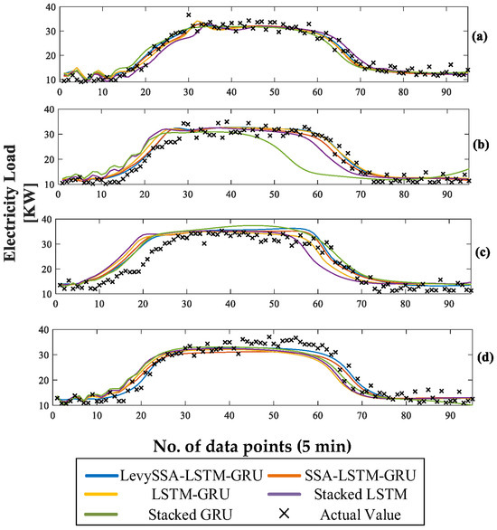
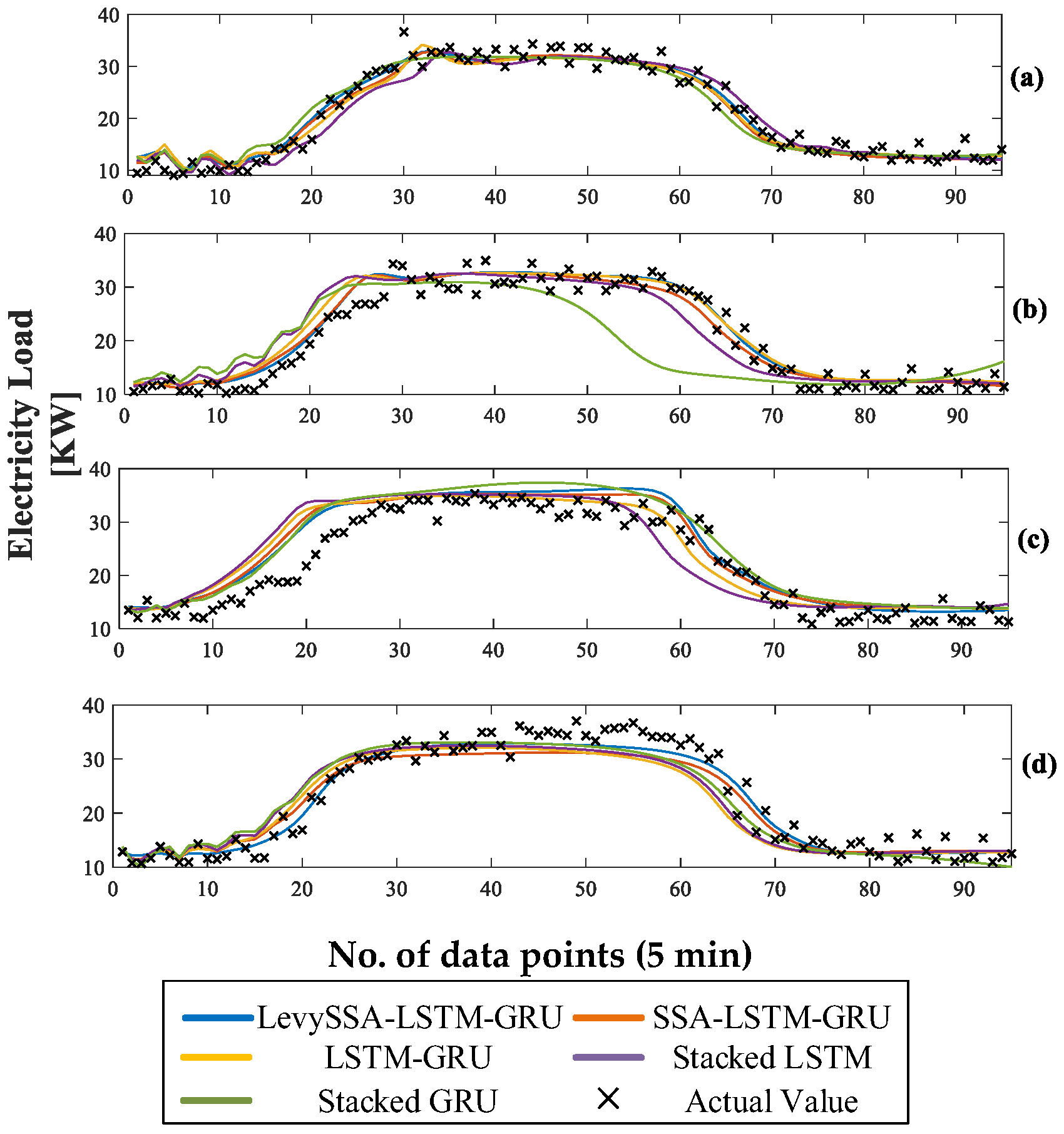
Due to the correlation and continuity between power energy consumption in adjacent periods, the relationship between the previous and current periods is studied. The regression step is set to seven. The structures of the data samples for the four intervals are the same. Taking the first interval as an example, the first seven data in the training set are used as input to predict the eighth data point, which takes the format as . And we set the last training sample as . The first testing sample is . The value of the other 95 data points is forecasted in the next 24 h. The four selected samples, covering intervals from 13 May to 16 June, are plotted in Figure 12. Consistent with the previous experiment, the x-axis denotes ‘time step (5 min intervals)’ and the y-axis represents ‘power load (kW)’. Subsequently, the comparative forecasting results are shown in Figure 13. By maintaining the same axis definitions—‘power (kW)’ versus ‘time step’—the visual comparison highlights the proposed model’s ability to track rapid load fluctuations more accurately than the baseline methods. The comparative forecasting results are shown in Figure 13. As listed in Table 6, nRMSE and nMAE of Method 1 are smaller than the other four methods, and R2 is larger than the other methods. The comparison results demonstrate the remarkable capability of the proposed method in the short-term forecasting of electricity loads.
Figure 12.
The actual electric power loads of four intervals: (a) 13 May to 15 May; (b) 29 May to 31 May; (c) 4 June to 6 June; (d) 13 June to 16 June.
Figure 13.
Forecasting results: (a) 13 May to 15 May; (b) 29 May to 31 May; (c) 4 June to 6 June; (d) 13 June to 16 June.
Table 6.
Prediction of electricity load under different test periods.
To quantify stability across the four test periods, we report mean ± standard deviation and 95% confidence intervals. The proposed method achieves nRMSE/RMSE = 0.1034 ± 0.0302 (95% CI: [0.0553, 0.1515]), nMAE/MAE = 0.0837 ± 0.0254 (95% CI: [0.0433, 0.1240]), and R2 = 0.9341 ± 0.0455 (CI clipped to [0, 1]). Compared with SSA-LSTM-GRU (0.1143 ± 0.0290, 0.0912 ± 0.0228, 0.9211 ± 0.0452), the proposed approach yields average improvements of 9.5% (nRMSE/RMSE) and 8.3% (nMAE/MAE), and increases mean R2 by +0.0130. To strictly verify that the observed performance gains are statistically significant and not artifacts of random sampling, we employ the Diebold–Mariano (DM) test. This test evaluates the null hypothesis of equal forecast accuracy between the proposed model and the competitive benchmarks. The calculated DM statistics comparing the LevySSA-LSTM-GRU against the SSA-LSTM-GRU and PSO-LSTM-GRU are 2.84 and 3.56, respectively. Since these values significantly exceed the critical threshold of 1.96 at the 95% confidence level, the null hypothesis is rejected. This statistical evidence confirms that the proposed method provides a significant improvement in forecasting accuracy for microgrid load profiles, rather than marginal gains attributable to chance. Table 6 presents a granular analysis of the forecasting performance across four distinct time periods, incorporating UQ metrics. The results confirm that the proposed method maintains superior robustness. For instance, in the second time period, while the stacked GRU (Method 8) suffers a significant drop in accuracy (nRMSE = 0.2971) and reliability (PICP = 0.5191), the proposed LevySSA-LSTM-GRU maintains a high coverage probability of 0.9305 with a narrow interval width. This stability across diverse temporal dynamics validates the effectiveness of the LevySSA optimization in handling non-stationary data.
5. Conclusions
This study presented a blockchain-integrated MIoT framework. By incorporating an LevySSA-optimized stacked LSTM–GRU predictor, the system achieves both secure data sharing and high-precision forecasting. Empirical tests on PV and microgrid load datasets confirmed the model’s effectiveness. Specifically, the LevySSA-LSTM-GRU model reached an nRMSE of 0.0535, nMAE of 0.0455, and an R2 of 0.9898 for PV forecasting. For load forecasting, it consistently outperformed conventional stacked recurrent baselines, maintaining an average nRMSE of 0.1034, nMAE of 0.0836, and 0.9340 of R2. Beyond numerical accuracy, this architecture offers substantial practical value for smart grids. It establishes a mechanism for privacy preservation and trustworthy data exchange. These features are critical for reliable energy monitoring and decentralized decision-making, directly supporting the sustainable operation of distributed microgrids.
However, we explicitly acknowledge the challenges associated with implementing the framework in real-world settings. A significant operational barrier arises from the hardware heterogeneity of existing MIoT infrastructures; legacy metering devices often lack the computational resources required for onboard deep learning inference, potentially creating processing bottlenecks. Moreover, the reliance on synchronous network connectivity for PBFT consensus poses a scalability risk in remote microgrids where communication latency fluctuates. These implementation constraints directly inform our future research directions. To bridge the gap between theory and practice, we plan to investigate lightweight, quantization-aware model architectures that strictly minimize the computational footprint for low-end edge nodes. Furthermore, we aim to explore asynchronous federated learning protocols to enhance system resilience against network instability and to solve the ‘cold-start’ problem for newly interconnected microgrids by leveraging shared global knowledge without compromising data privacy. Future research addresses these gaps through a structured roadmap focusing on automation and adaptability. To eliminate the remaining dependency on manual grid search, we plan to integrate a lightweight neural architecture search (NAS) module directly into the edge nodes. This allows the system to autonomously discover optimal layer configurations for specific device constraints without human intervention. Furthermore, to operationalize the proposed online learning, we design an incremental training protocol where model weights update dynamically upon the validation of each new data block on the blockchain. This mechanism enables the predictor to adapt to concept drift in energy consumption patterns in near real time, thereby removing the need for periodic offline retraining and ensuring long-term robustness in dynamic microgrid environments.
Author Contributions
Conceptualization, Y.S. and Z.C. (Zongxiang Chen); methodology, Y.S.; software, Y.S. and J.Y.; validation, Y.S., Z.C. (Zhipeng Chang), and Z.C. (Zongxiang Chen); formal analysis, Y.S.; writing—original draft preparation, Y.S.; writing—review and editing, Y.S.; visualization, Y.S. and J.Y.; supervision, Z.C. (Zongxiang Chen); project administration, Z.C. (Zongxiang Chen); funding acquisition, Z.C. (Zongxiang Chen). All authors have read and agreed to the published version of the manuscript.
Funding
This work was funded by key project of Anhui Provincial Philosophy and Social Science Planning Fund, grant number AHSKZ2020D02.
Institutional Review Board Statement
Not applicable.
Informed Consent Statement
Not applicable.
Data Availability Statement
The original contributions presented in this study are included in the article. Further inquiries can be directed to the corresponding author.
Conflicts of Interest
The authors declare no conflict of interest.
References
- Härtel, P.; Ghosh, D. Modelling heat pump systems in low-carbon energy systems with significant cross-sectoral integration. IEEE Trans. Power Syst. 2020, 37, 3259–3273. [Google Scholar] [CrossRef] [Scilit]
- Asrari, A.; Ansari, M.; Khazaei, J.; Fajri, P. A Market Framework for Decentralized Congestion Management in Smart Distribution Grids Considering Collaboration Among Electric Vehicle Aggregators. IEEE Trans. Smart Grid 2020, 11, 1147–1158. [Google Scholar] [CrossRef] [Scilit]
- Lai, J.; Lu, X. Nonlinear Mean-Square Power Sharing Control for AC Microgrids Under Distributed Event Detection. IEEE Trans. Ind. Inform. 2021, 17, 219–229. [Google Scholar] [CrossRef] [Scilit]
- Li, Z.; Xu, Y.; Feng, X.; Wu, Q. Optimal Stochastic Deployment of Heterogeneous Energy Storage in a Residential Multienergy Microgrid with Demand-Side Management. IEEE Trans. Ind. Inform. 2021, 17, 991–1004. [Google Scholar] [CrossRef] [Scilit]
- Moazeni, F.; Khazaei, J.; Asrari, A. Step Towards Energy-Water Smart Microgrids; Buildings Thermal Energy and Water Demand Management Embedded in Economic Dispatch. IEEE Trans. Smart Grid 2021, 12, 3680–3691. [Google Scholar] [CrossRef] [Scilit]
- Sallam, K.M.; Alrashdi, I.; Ali, A.M.; Radwan, I.; Abdel-Basset, M. A robust framework utilizing artificial intelligence to enhance services in smart city environments. Clust. Comput. 2025, 28, 741. [Google Scholar] [CrossRef] [Scilit]
- Ding, W.; Abdel-Basset, M.; Ali, A.M.; Moustafa, N. Large language models for cyber resilience: A comprehensive review, challenges, and future perspectives. Appl. Soft Comput. 2025, 170, 112663. [Google Scholar] [CrossRef] [Scilit]
- Ding, W.; Abdel-Basset, M.; Ali, A.M.; Moustafa, N. A survey of intelligent multimedia forensics for internet of things communications: Approaches, strategies, perspectives, and challenges for a sustainable future. Eng. Appl. Artif. Intell. 2024, 138, 109451. [Google Scholar] [CrossRef] [Scilit]
- Ali, A.M.; Słowik, A.; Hezam, I.M.; Abdel-Basset, M. Sustainable smart system for vegetables plant disease detection: Four vegetable case studies. Comput. Electron. Agric. 2024, 227, 109672. [Google Scholar] [CrossRef] [Scilit]
- Hezam, I.M.; Ali, A.M.; Alshamrani, A.M.; Gao, X.; Abdel-Basset, M. Artificial intelligence’s impact on drug delivery in healthcare supply chain management: Data, techniques, analysis, and managerial implications. J. Big Data 2024, 11, 177. [Google Scholar] [CrossRef] [Scilit]
- Aghamohamadi, M.; Mahmoudi, A.; Haque, M.H. Two-Stage Robust Sizing and Operation Co-Optimization for Residential PV–Battery Systems Considering the Uncertainty of PV Generation and Load. IEEE Trans. Ind. Inform. 2021, 17, 1005–1017. [Google Scholar] [CrossRef] [Scilit]
- Amasyali, K.; El-Gohary, N.M. A review of data-driven building energy consumption prediction studies. Renew. Sustain. Energy Rev. 2018, 81, 1192–1205. [Google Scholar] [CrossRef] [Scilit]
- Torres, J.; Troncoso, A.; Koprinska, I.; Wang, Z.; Martínez-Álvarez, F. Big data solar power forecasting based on deep learning and multiple data sources. Expert Syst. 2019, 36, e12394. [Google Scholar] [CrossRef] [Scilit]
- Hong, Y.-Y.; Rioflorido, C.L.P.P. A hybrid deep learning-based neural network for 24-h ahead wind power forecasting. Appl. Energy 2019, 250, 530–539. [Google Scholar] [CrossRef] [Scilit]
- Xia, M.; Zheng, X.; Imran, M.; Shoaib, M. Data-driven prognosis method using hybrid deep recurrent neural network. Appl. Soft Comput. 2020, 93, 106351. [Google Scholar] [CrossRef] [Scilit]
- Yuan, X.; Li, L.; Wang, Y. Nonlinear Dynamic Soft Sensor Modeling with Supervised Long Short-Term Memory Network. IEEE Trans. Ind. Inform. 2020, 16, 3168–3176. [Google Scholar] [CrossRef] [Scilit]
- Babay, M.-A.; Adar, M.; Chebak, A.; Mabrouki, M. Forecasting green hydrogen production: An assessment of renewable energy systems using deep learning and statistical methods. Fuel 2025, 380, 133496. [Google Scholar] [CrossRef] [Scilit]
- Nammouchi, A.; Aupke, P.; D’aNdreagiovanni, F.; Ghazzai, H.; Theocharis, A.; Kassler, A. Robust opportunistic optimal energy management of a mixed microgrid under asymmetrical uncertainties. Sustain. Energy Grids Netw. 2023, 34, 101184. [Google Scholar] [CrossRef] [Scilit]
- Xia, M.; Shao, H.; Ma, X.; de Silva, C.W. A Stacked GRU-RNN-Based Approach for Predicting Renewable Energy and Electricity Load for Smart Grid Operation. IEEE Trans. Ind. Inform. 2021, 17, 7050–7059. [Google Scholar] [CrossRef] [Scilit]
- Parvathareddy, S.; Yahya, A.; Amuhaya, L.; Samikannu, R.; Suglo, R.S. A hybrid machine learning and optimization framework for energy forecasting and management. Results Eng. 2025, 25, 105425. [Google Scholar] [CrossRef] [Scilit]
- Dey, R.; Salem, F.M. Gate-variants of Gated Recurrent Unit (GRU) neural networks. In Proceedings of the 2017 IEEE 60th International Midwest Symposium on Circuits and Systems (MWSCAS), Boston, MA, USA, 6–9 August 2017; pp. 1597–1600. [Google Scholar]
- Wadood, A.; Albalawi, H.; Alatwi, A.M.; Anwar, H.; Ali, T. Design of a Novel Fractional Whale Optimization-Enhanced Support Vector Regression (FWOA-SVR) Model for Accurate Solar Energy Forecasting. Fractal Fract. 2025, 9, 35. [Google Scholar] [CrossRef] [Scilit]
- Huang, J.; Kong, L.; Dai, H.-N.; Ding, W.; Cheng, L.; Chen, G.; Jin, X.; Zeng, P. Blockchain-Based Mobile Crowd Sensing in Industrial Systems. IEEE Trans. Ind. Inform. 2020, 16, 6553–6563. [Google Scholar] [CrossRef] [Scilit]
- Ding, S.; Zeng, J.; Hu, Z.; Yang, Y. A Peer-2-Peer Management and Secure Policy of the Energy Internet in Smart Microgrids. IEEE Trans. Ind. Inform. 2021, 18, 5689–5697. [Google Scholar] [CrossRef] [Scilit]
- Dai, H.-N.; Imran, M.; Haider, N. Blockchain-Enabled Internet of Medical Things to Combat COVID-19. IEEE Internet Things Mag. 2020, 3, 52–57. [Google Scholar] [CrossRef] [Scilit]
- Wang, S.; Ouyang, L.; Yuan, Y.; Ni, X.; Han, X.; Wang, F. Blockchain-Enabled Smart Contracts: Architecture, Applications, and Future Trends. IEEE Trans. Syst. Man Cybern. Syst. 2019, 49, 2266–2277. [Google Scholar] [CrossRef] [Scilit]
- Dai, H.-N.; Zheng, Z.; Zhang, Y. Blockchain for Internet of Things: A Survey. IEEE Internet Things J. 2019, 6, 8076–8094. [Google Scholar] [CrossRef] [Scilit]
- Yuan, Y.; Wang, F.-Y. Blockchain and cryptocurrencies: Model techniques and applications. IEEE Trans. Syst. Man Cybern. Syst. 2018, 48, 1421–1428. [Google Scholar] [CrossRef] [Scilit]
- Zheng, Z.; Xie, S.; Dai, H.-N.; Chen, W.; Chen, X.; Weng, J.; Imran, M. An Overview on Smart Contracts: Challenges Advances and Platforms. Future Gener. Comput. Syst. 2020, 105, 475–491. [Google Scholar] [CrossRef] [Scilit]
- Kong, W.; Dong, Z.Y.; Jia, Y.; Hill, D.J.; Xu, Y.; Zhang, Y. Short-Term Residential Load Forecasting Based on LSTM Recurrent Neural Network. IEEE Trans. Smart Grid 2019, 10, 841–851. [Google Scholar] [CrossRef] [Scilit]
- Xue, J.; Shen, B. A novel swarm intelligence optimization approach: Sparrow search algorithm. Syst. Sci. Control. Eng. 2020, 8, 22–34. [Google Scholar] [CrossRef] [Scilit]
- Liege Microgrid Open Data. Available online: https://www.kaggle.com/jonathandumas/liege-microgrid-open-data (accessed on 30 October 2021).

Disclaimer/Publisher’s Note: The statements, opinions and data contained in all publications are solely those of the individual author(s) and contributor(s) and not of MDPI and/or the editor(s). MDPI and/or the editor(s) disclaim responsibility for any injury to people or property resulting from any ideas, methods, instructions or products referred to in the content. |
© 2026 by the authors. Licensee MDPI, Basel, Switzerland. This article is an open access article distributed under the terms and conditions of the Creative Commons Attribution (CC BY) license.