Investigation of the Importance of Asphalt Mixing Plant Properties for Selecting the Best Sustainable Alternative

Abstract

The optimal composition of an asphalt mixture, composed from the various mineral materials and bituminous binders, is produced in an asphalt mixing plant (AMP). Various AMP properties determine the suitability of this complex, long-term-use technological equipment in meeting contemporary requirements. Worn AMPs are replaced with new ones when they fail to satisfy these requirements. The AMP purchase process consists of two separate parts: (1) the decision-making process—whether there is a need to purchase a new AMP; and (2) AMP suitability—the evaluation of various technical and other properties, related to the AMP itself. This research paper considers the second part of the AMP purchase process and presents a new twenty-criteria system that identifies the most important AMP quality parameters indicating AMP suitability. The weights of the quality criteria for a new AMP were established by applying the Average Rank Transformation into Weight-Linear (ARTIW-L), Non-Linear (ARTIW-N) and Analytic Hierarchy Process (AHP) methods. Furthermore, the paper presents and verifies the Inverse Hierarchy for Assessment of Main Criteria Importance (IHAMCI) method. The findings of the research show that customers consider technological parameters to be the most important, followed by technical performance. Economical indicators rank third, while ecological (environmental) indicators receive the least attention. Future research will assess the sustainability requirements applied to operating AMPs in recent years.

1. Introduction

During the construction of various roads, ports, airport runways, or other traffic areas, various types of asphalt mixing plants (AMPs) are used to produce asphalt mixture. According to Zapata & Gambatese [1], nearly 90% of paved roads worldwide are made of asphalt mixtures, which ensures sufficient roughness and adhesion with interacting road transport [2]. For the use of asphalt or bituminous materials, sub-ballast has emerged as a proven solution for improving railway performance and durability [3]. However, other pavement types (e.g., gravel or unpaved road) cause various ride-related issues and negative factors for surrounding residents [4]. In 2022, the total asphalt production in Europe reached 269 million tonnes [5], while the global asphalt market size is expected to reach USD 321.5 million in 2027 [6]. Due to the steady growth of the asphalt market and advancement in the road construction industry, the demand for asphalt mixtures and AMPs is constantly increasing [7]. The range of currently available AMP types and models is notably wide, for example: stationary-type AMPs, mobile-type AMPs, batch-mix-type AMPs, drum-mix-type AMPs, small-type AMPs, hot-mix-type AMPs, and cold-mix-type AMPs [8]. When comparing these different APM’s types, it should be noted that they exhibit distinct performance features and advantages/disadvantages (e.g., high mixing quality, long service life, simple operation, etc.) and are suited to different road construction engineering. Consequently, both AMP selection and operation directly affect pavement quality. For this reason, performance requirements for AMPs continue to increase. As a result, many researchers have focused on analyzing AMP performance indicators, features, and production processes related to hot-mix asphalt (HMA) mixtures [9,10]. This section provides a concise review of research on the analysis of AMP performance indicators and HMA production processes.

Firstly, energy consumption can be identified as a key performance indicator and is frequently discussed by scholars. According to Xie et al. [11], the problematic nature of the relation between road construction and energy consumption is evident, as road construction accounts for approximately 28% of global energy consumption. For this reason, when applying various research approaches—such as energy consumption monitoring, analytical methods, or comparative studies—researchers seek new ways to improve energy efficiency in road construction processes [11,12,13,14]. For example, Androjić & Alduk [13] concluded that reducing the production temperature of hot-mix asphalt (HMA) leads to lower energy consumption during production. In addition, with regard to the temperature, Thives & Ghisi [15] stated that due to reduced mixing temperature, the use of warm-mix asphalt (WMA) technologies can reduce energy consumption compared to the HMA. Zaumanis et al. [16] also reported that WMA technologies allow for lowering the production and pavement temperature of the HMA, thus reducing energy demand. Moreover, after conducting a life cycle assessment, the authors developed a tool to assess the energy demand of the WMA. However, temperature is not the only factor that directly affects the energy consumption. According to Androjić & Alduk [13], the energy required for HMA production also depends on factors such as the moisture content of the mineral mixture, production delays, AMP properties and technical features, and the quality of the fuel used. The authors concluded that increasing production capacity utilization and decreasing moisture content and production temperature of asphalt mix can result in significant energy savings. Energy reduction during HMA production was also discussed by Grabowski et al. [17], who emphasized the importance of organizational changes in AMP production and management systems. Appropriate organizational improvements may lead to reduced energy consumption in HMA production without additional financial costs. Furthermore, Sukhija et al. [18] investigated the use of additives categorized as organic-, chemical-, and foaming-based technologies to reduce energy consumption. The achieved results demonstrated that the addition of the WMA additives lowers the energy consumption by 3–12% compared to HMA. According to Cimbola et al. [19], despite numerous efforts to rationalize energy consumption in road construction processes, a key challenge remains in further developing production processes that are both environmentally friendly and energy-efficient. Therefore, considering the extensive research aimed at reducing energy consumption in road construction, energy consumption should be regarded as one of the key criteria when comparing different AMP types and when selecting an AMP for purchase.

Secondly, a significant number of studies consider emissions to be an important sustainability indicator of AMP performance and the HMA production process. The environmental impact of road construction is closely associated with increased greenhouse gas (GHG) emissions, which are strongly linked to climate change [20]. Therefore, GHG emissions can be used as a key criterion for environmental evaluation [21]. Emissions generated by the asphalt industry have recently gained increased attention, particularly after the National Asphalt Pavement Association announced its goal of achieving net-zero carbon emissions by 2050 [22]. According to Le Guen et al. [23], HMA production offers a serious research challenge while seeking to reduce emissions within the road construction industry. Addressing this challenge, Espinoza et al. [20] emphasized that special attention must be paid to HMA production in order to minimize GHG emissions. The authors therefore recommended increasing the efficiency of asphalt mixing equipment and construction techniques. Moreover, they noted that the use of raw materials such as reclaimed asphalt pavement (RAP) can contribute to emission reductions [20]. In order to reduce pollutant emissions, three new asphalt modifiers were developed and added to the asphalt mixtures [24]. The achieved results were positive; however, the authors noticed that the emission reduction performance of HMA is affected by the technical properties of the AMP (asphalt binder type) and mixture gradation. Regarding different types of AMPs, Santos et al. aimed to quantify and compare the emissions in different AMPs (batch or drum mix, production capacity, mobile or fixed, etc.) [25]. It was found that energy demand and generated emissions per ton vary significantly among different AMP models. When comparing emissions produced by various AMP types or during different stages of asphalt production, researchers often focus on how to properly and quantitatively evaluate greenhouse gas (GHG) emissions [26,27]. For example, in order to evaluate the effect of WMA emission reduction, Qin & Sun [28] proposed a novel method which showed that the effect of WMA improvement on the emissions is related to the of asphalt mixture production stage rather than the construction stage. The quantification of the GHG emission at the construction stage is described by Wang et al. [26]. It should be noted that WMA represents a significant opportunity for the asphalt industry to improve product performance, construction efficiency, and environmental stewardship [29]. Considering the reviewed studies, it is evident that the asphalt industry is making continuous efforts to reduce emissions as concerns about global warming increase, and that emission levels can no longer be ignored. Furthermore, because different AMP types generate different amounts of emissions, emission performance should be regarded as a key criterion when selecting an asphalt mixing plant.

Thirdly, the asphalt industry faces ongoing pressure to optimize the use of available resources as the cost of both materials and transport increase fuel prices. Consequently, researchers also focus on economic aspects, production costs, asphalt mixture quality, and other technical properties of the AMPs. The properties of the designed asphalt mixture must meet the requirements for technical specifications while simultaneously minimizing cost [30]. The overall performance of the HMA mixture depends on its composition, including the properties, proportions and distribution of the ingredients [31]. The gradation of the aggregate is one of the most important parameters for the technical properties of the HMA; therefore, determining the gradation of the aggregate is one of the key topics of civil engineering [32]. Shen & Yu [33] analyzed aggregate packing and applied discrete element modelling to relate aggregate gradation characteristics to the voids in the mineral aggregate of HMA. In their study, a new classification for traditional dense-graded aggregate gradation was proposed, consisting of coarse-, medium-, and fine-graded categories. Zulkati et al. [34] investigated the role of filler in the mechanical performance of the asphalt concrete mixture. Three wearing course mixtures incorporating granite, hydrated lime, and coal as filler fractions were evaluated using the Marshall mix design method to determine the optimum use of the bituminous binder. The results revealed that fillers in asphalt concrete mixtures influence performance in three key ways: they alter the required bituminous binder quantity, affect workability during mixing and compaction, and enhance overall mixture properties through the bitumen-filler mastic. Furthermore, industrialists are also focusing their efforts on both increasing the recycling rates and reducing the temperatures required to produce recycled asphalt concrete. Producing hot-mix recycled asphalt concrete in plants is one of the available techniques to perform cost- and environmentally effective pavement recycling [35]. The main objective is to optimize the manufacturing process while maintaining the same production quality as that achieved through traditional production at 160 °C without the use of reclaimed asphalt pavement (RAP). The study conducted by Mogawer et al. [36] aimed to evaluate the effects of plant type (batch and drum) and production parameters on stiffness, performance, and degree of blending between the aged and virgin binders in plant-produced RAP mixtures. Mixtures produced in both batch and drum plants, along with corresponding production data, were analyzed. The most commonly used approach for incorporating RAP into the asphalt production involves superheating virgin aggregates so that, upon contact, they dry and heat the RAP through conduction. This method prevents direct exposure of RAP to flame. The required superheating temperature depends on the content, moisture, and required discharge temperature of the RAP. According to Zaumanis et al. [16], establishing asphalt plants capable of recycling 100% of RAP could significantly increase recycling capacity and reduce the amount of RAP diverted to low-value applications. As demonstrated by the reviewed studies, various technical features and performance capabilities of AMPs should be carefully considered when planning the purchase of a new asphalt mixing plant.

The quality of the HMA mixtures, environmental contamination, pollution, company’s economic efficiency and ability to meet user demands for HMA mixtures all depend on the quality of the AMP [37]. As there are many possible demands and requirements, it must be noted that AMP properties do not always satisfy these demands and requirements. Whether the AMP meets specific demands and requirements often depends on the user’s priorities, intended mode of operation, and the degree of attention paid to technical specifications and quality-related parameters during the purchasing process. Even AMP manufacturers recommend that potential buyers carefully assess their needs and priorities before purchasing [8]. Therefore, to avoid ill-considered AMP purchases, inefficient utilization of new plants, and financial losses, a comprehensive and systematic quality evaluation framework for AMP selection is essential. From this perspective, the AMP purchasing process can be divided into two main stages: 1. decision-making process—whether there is or there is no need to buy a new AMP, and 2. suitability of the AMP—evaluation of various technical and other properties related to the AMP itself. As the decision-making process for purchasing a new AMP and renewing the AMP fleet has already been described by the authors of this research paper [38], the present work represents a continuation of that research and focuses on evaluating various AMP properties relevant to the purchasing decision.

For this reason, the aim of this paper is to introduce an innovative system of quality criteria for asphalt mixing plants (AMPs) by employing multiple-criteria decision-making (MCDM) methods [39] to determine the significance of the criteria, sub-criteria and main criteria that influence an asphalt production company’s decision to purchase a new AMP, while considering various AMP properties.

2. Materials and Methods

2.1. Definition of the Quality Criteria for the AMPs

Based on the analyzed literature, technical product catalogues, and consultations with AMP manufacturers, the most important properties and features of the AMPs were identified, ranging from plant type to esthetic aspects. Considering these key properties and features, an innovative system comprising 20 criteria (indicators) was developed to enable a comprehensive evaluation of AMP quality. This system assists potential buyers in deciding whether to purchase a specific AMP model or to select a more suitable alternative. The criteria-based evaluation system is described below:

• Type and manufacturer of the AMP (PTM)—the type of the AMP (batch plant, continuous mix plant, drum-mix plant, stationary, mobile or wheel-mounted mobile plant) and the manufacturer’s brand.
• Price, discount, warranty (PDW)—the price of the AMP, flexibility of the discount system, duration of the warranty period, and cost of spare parts.
• Plant capacity at 5% aggregate moisture (PCM)—the maximum technical capacity of the AMP (production rate) under conditions of low, average, and high aggregate moisture content.
• Design of the drying drum and type of burner (DDT)—the design of the dryer drum (contra-flow or parallel-flow), heat insulation, type of fuel (natural gas, extra light fuel, heavy oil, brown-coal dust), and burner type.
• Efficiency of dust collection (EDC)—the efficiency of dust collection (baghouse) from air and gas flow, the design of equipment (dry or wet, two- or three-fold), the possibility of separate reclaimed dust storage and batching with imported filler.
• Sampling of hot aggregates (SHA)—the possibility of comfort sampling from separate aggregate fractions within the hot bin and other technological equipment of the AMP for factory production control.
• Type and effectiveness of the mixer (TEM)—the type of mixer (forced or gravity mixer), the maximum weight of one HMA mixture batch, and the minimum mixing duration required to achieve proper homogeneity of the HMA mixture.
• Facility for the reclaimed asphalt (FRA)—the capability to receive, store and accurately batch RAP and reclaimed asphalt shingles (RAS) into the mixer or other AMP equipment.
• Facility to mix additives (FMA)—the capability to receive, store and accurately batch additives, including fibres (arbocel), granulates (polyethylene, craton) and liquids (wet fix, eterlen, rejuvenator).
• Occupied (required) area and height of the AMP (OAH)—the total area occupied by the general dimensions of the AMP equipment and the height of the AMP (mixing tower, chimney, reclaimed dust and imported filler silo), which determines the type of the mounted crane, hoist duty and lifting height.
• Noise, vibration, and gas ejection (NVE)—the level of noise and vibration, the intensity of vapour (gas) dispersion from the bituminous binder and dryer drum, generated GHG emissions.
• Control system accuracy (CSA)—the precision and reliability of the asphalt mixture production process, including the capabilities of the computerized control system, data tracking, and maintenance functions.
• Bitumen batching system (BBS)—the design of the storage tank, transportation, and batching system (by volume or weight) of the bituminous binder, used technique to pump down the portioned bitumen into the mixer (pressure drop or gravitation—by using a high-intensity stream), inaccuracies in the bitumen batching process.
• Supplementary equipment possibility (SEP)—the possibility of integrating supplementary equipment without alterations to the standard design of the AMP: RAP parallel drum, additive fibre granule feed, cold aggregate feeders, HMA mixture storage silo, bitumen tanks designed for the polymer-modified binder.
• HMA storage silo parameters (SSPs)—the location of the storage silo of the manufactured HMA mixture (under or beside the tower), the number of compartments and its volume, heat insulation efficiency, equipment for reducing mixture segregation, and the ability to load HMA into trucks.
• Electricity and fuel consumption (EFC)—the amount of electricity and fuel required to produce one tonne of HMA mixture.
• Number of cold aggregate feeders (CAFs)—the number and volume of cold aggregate bins, rapid changes in feeder capacity, possibility to remove aggregate remains from the bins, the range of adjusting feeder output performance.
• Number of screen decks and the volume of the hot aggregate bin (HSB)—the number of hot screened aggregate fractions, the volume of compartments in the hot bin, screening effectiveness at maximum output, the capability to store non-screened mix (bypass), inaccuracies in hot fraction batching.
• Mounting, balancing, and maintenance (MBM)—the options for AMP delivery, installation, balancing and maintenance.
• Esthetics of the AMP and its visual pollution (AVP)—the esthetics (exterior colour combinations, graphics), environmental friendliness of the AMP, visual pollution.

As shown below, all twenty proposed criteria can be grouped into four main criteria: technical performance, technological parameters, economical indices, and ecological indices. Considering the 11 core environmental impact categories of EN 15804, the criteria analyzed in this research are directly associated with E, K, and T, and indirectly associated with D, L, and P.

2.2. Experts Team Selection

To apply the MCDM methods and determine the relative importance of each proposed criteria for potential AMPs buyers, an experimental evaluation was conducted. A group of 30 experts was asked to complete prepared questionnaires by ranking the criteria. The experts included asphalt mixture production managers from road construction companies, representatives of AMP sales and maintenance companies, AMP operators, and researchers. The experts were given a period of more than one year to fill out the questionnaire. In the absence of the hierarchical structure, all of the criteria in the questionnaire were randomly presented, giving them alphanumeric characters, full descriptions, and abbreviations. All 30 questionnaires were filled out correctly; therefore, it can be stated that the experimental evaluation was successful as the number of completed questionnaires was 1.5 times higher than the number of criteria. The average rankings of the criteria were calculated. The consistency of the expert opinions was verified by applying the concordance coefficient $W$ [40].

2.3. Models of Hierarchical Criteria

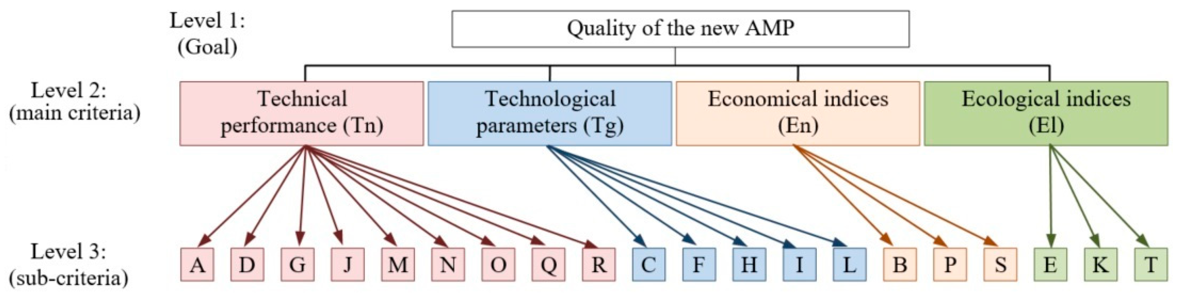
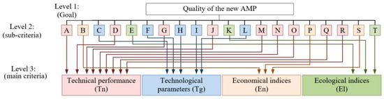
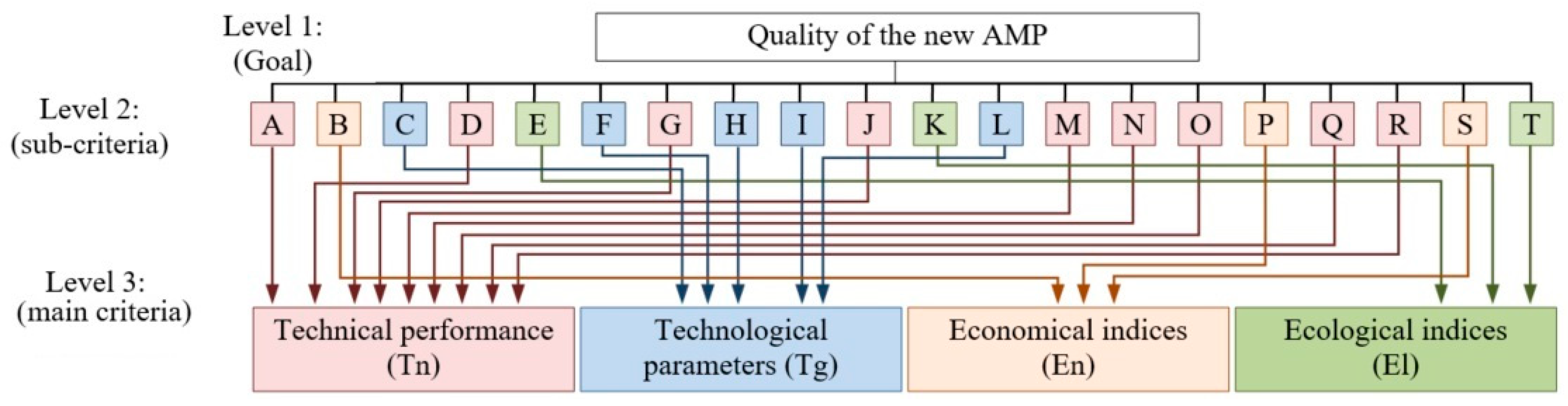
Due to the large number of criteria, their normalized subjective global weights were calculated in two ways: directly, i.e., when all of the criteria were not attributed to any of the groups (Figure 1), and using a hierarchical structure (Figure 2). Finally, the IHAMCI (Inverse Hierarchy for Assessment Main Criteria Importance) method was applied. The application of the IHAMCI method allowed the sub-criteria to be taken into account, which were divided into certain groups, and the normalized weights of the main criteria were calculated (Figure 3).

Figure 1. The model of quality criteria system when the criteria are not divided according to the hierarchical structure.

Figure 2. The three-level direct hierarchical model of the quality criteria system.

Figure 3. The three-level inverse hierarchical model of the quality criteria system.

The results of criteria evaluation by a group of experts (IHAMCI method) are more reliable than the results obtained from a single expert. Moreover, the relative weights of the main criteria calculated from the global criteria weights are obtained by initially comparing all criteria with each other rather than comparing their groups, which improves the consistency of the evaluation.

2.4. Application of the MCDM Methods

The weights of the AMP criteria have a significant effect on the outcome of multi-criteria evaluation and on the overall accuracy of the decision-making process. In practice, the most commonly used subjective weights are those established by experts. The subjective weights of the criteria of the research object (in this case—AMP) indicate the opinion of qualified experts who have extensive theoretical and practical experience and specific knowledge in the field of investigation [41].

The subjective weights of the criteria can be determined from the ranks assigned by experts to these criteria. The opinions of individual experts are often inconsistent and sometimes even contradictory; that is, the perceived importance of criteria may differ fundamentally among experts. The results of the evaluation depend on the experts’ qualification, their knowledge of the research object, their responsibility in assigning numerical importance values to the criteria, and their willingness to participate in the research. Since expert opinions on the relative importance and priorities of criteria often vary, the ranks or weights can be used in multi-criteria evaluation as generalized representations of the expert group’s collective opinion, provided there is sufficient evidence of consistency among all expert evaluations. When decisions are based on the average evaluations of experts, it is necessary to assess the degree of agreement in their opinions by determining the concordance coefficient.

For experts, it is easier to assign ranks to the criteria while considering their relative importance. This ranking method for determining criterion importance is simple but not highly precise, making it most suitable for the initial stage of research. However, even when applying more accurate and sophisticated methods to determine criterion weights, it is still recommended to begin with rank assignment. The weights of the ranked criteria can then be calculated using various approaches, although no single method has a theoretical advantage over the others. The general principle across all approaches is the same: the most important criterion should be assigned the highest weight. The weights values must meet the ranks of the criteria, and the sum of the weights of all criteria must be equal to 1.

2.5. ARTIW-L and ARTIW-N Methods for Determination of the AMP Criteria Weights

The ranks assigned to the criteria by the expert group can be readily converted into weights by using the ARTIW-L and ARTIW-N methods. Detailed instructions for applying the ARTIW-L method can be found in [42]. The weights of the criteria calculated using this method are inversely linearly linked to the average ranks of these criteria.

The application of the average criterion rank ${\overline{R}}_i$ while seeking to determine the importance of the AMP criteria leads to an inconvenient result—the more important the criterion is, the lower its ${\overline{R}}_i$ is. For practical purposes, it is preferable to express criterion importance numerically so that higher values correspond to greater importances. Thus, normalized relative weights ${\omega }_i^{ARTIW-L}$ indicating the relative importance of the criteria are used and are calculated according to the following formula:

$${\omega }_i^{ARTIW-L}={\displaystyle \frac{\left(m+1\right)-\overline{R_i}}{{\sum }_{i=1}^m\overline{R_i}}}$$

(1)

where $m$ represents the number of criteria showing the quality (properties) of the AMP $\left(i=1, 2, \dots ,m\right).$ ${\overline{R}}_i$ represents the average criterion rank assigned to each i-th criterion of the AMP:

$$\overline{R_i}={\displaystyle \frac{{\sum }_{e=1}^n{R}_{ie}}{n}}={\displaystyle \frac{R_i}{n}}$$

(2)

where $n$ represents the number of the experts who evaluated the importance of the AMP criteria $\left(e=1, 2, \dots ,n\right)$, and $R_{ie}$ represents the rank assigned to the i-th criterion by the e-th expert.

AMP properties (criteria normalized relative weights) ${\omega }_i^{ARTIW-N}$ can also be calculated using the ARTIW-N (Average Rank Transformation into Weight—Non-Linear) method [43,44]:

$${\omega }_i^{ARTIW-N}={\displaystyle \frac{\underset{i}{\min }\overline{R_i}}{{\overline{R}}_i·x{\sum }_{i=1}^m\frac{\underset{i}{\mathit{min}}\overline{R_i}}{\overline{R_i}}}}$$

(3)

where $\underset{i}{\min }\overline{R_i}$—the average rank of the most significant criterion (the smallest one); the ration $\underset{i}{\min }\overline{R_i}/{\overline{R}}_i$ is referred to as u_i in the following text.

The weights of the criteria calculated using this method are inversely linked to the average ranks of these criteria.

After calculating the weights of the criteria, it is also important to ensure that the expert opinions on the evaluation of the importance of AMP are consistent. The consistency in expert opinions is determined by calculating the Kendall’s concordance coefficient $W$. The sum of squares S of the deviations of the sum of criteria ranks ${\sum }_{e=1}^n{R}_{ie}$ from the general average of ranks $\overline{R}={\displaystyle \frac{n\left(m+1\right)}{2}}$ is calculated according to the following formula:

$$S=\sum _{i=1}^m{\left(R_i-\overline{R}\right)}^2=\sum _{i=1}^m{\left[\sum _{e=1}^n{R}_{ie}-{\displaystyle \frac{1}{2}}n\left(m+1\right)\right]}^2,$$

(4)

where $R_i$ represents the sum of the ranks of each i-th criterion equal to

$$R_i=\sum _{e=1}^n{R}_{ie}.$$

(5)

The total average of the ranks $\overline{R}$ of every criterion is obtained by dividing the sum of ranks given by experts from the number of the criteria $m$:

$$\overline{R}={\displaystyle \frac{{\sum }_{i=1}^m{\sum }_{e=1}^n{R}_{ie}}{m}}={\displaystyle \frac{n\left(m+1\right)}{2}}.$$

(6)

If $S$ is the actual sum of squares calculated according to Formula (4), the concordance coefficient $W$, in the absence of tied ranks, is defined by the ratio of $S$ and corresponding maximum $S_{\mathrm{m}\mathrm{a}\mathrm{x}}$ [40]:

$$W={\displaystyle \frac{12S}{n^2\left(m^3-m\right)}}.$$

(7)

When the opinions of the experts are consistent, the value of the concordance coefficient $W$ is close to 1, and if the differences between the opinions are large, the value of $W$ is close to 0.

It has been proved by Kendall [40] and Santos et al. [35] that if the number of the criteria is $m>7$, the importance of the concordance coefficient $W$ can be set by using Chi-Square distribution ${\chi }^2$:

$${\chi }^2=Wn\left(m-1\right)={\displaystyle \frac{12S}{nm\left(m+1\right)}}.$$

(8)

The random variable of Pearson’s criterion is dispersed according to the distribution ${\chi }^2$, while having a degree of freedom $\nu =m-1$. While considering the selected level of significance $\alpha$, the critical value ${\chi }_{v,\alpha }^2$ can be found from the ${\chi }^2$ distribution table with a degree of freedom $\nu$. Usually, in practice, the value $\alpha$ is accepted to be 0.05 or even higher −0.01. If the value of ${\chi }^2$ calculated according to the Formula (8) is higher than ${\chi }_{v,\alpha }^2$, it can be stated that the expert evaluations are consistent and that the estimated average criterion ranks ${\overline{R}}_i$ and weights of the criteria ${\omega }_i$ can be considered as the estimates of the significance of the criteria for the research object.

The lowest value of the concordance coefficient $W$ can be calculated as

$$W_{\min }={\displaystyle \frac{{\chi }_{v, \alpha }^2}{n\left(m-1\right)}},$$

(9)

where ${\chi }_{v,\alpha }^2$ represents critical Pearson’s statistics and the Chi-Square value, found in the table under the degree of freedom $v=m-1$ and level of significance $\alpha$.

If the calculated value of $W$ is higher than the lowest value of $W_{\mathrm{m}\mathrm{i}\mathrm{n}}$, the evaluations of the experts can be considered as consistent, also it can be considered that ${\overline{R}}_i$ and ${\omega }_i$ properly shows the importance of the criteria of the research object.

2.6. AHP Method for Determination of the AMP Criteria Weights

The weights of the criteria for the research object, as provided by a single expert, and the consistency of their opinion are typically determined by applying the Analytic Hierarchy Process (AHP) method [45,46]. The rank correlation method [40] is applied to determine the consistency in the opinions of the experts group. For this purpose, the weights of the criteria obtained from the expert group via the AHP method are converted into ranks, which are then used to calculate the concordance coefficient.

The AHP is a measurement theory based on pairwise comparisons and expert judgments, used to derive priority scales that assess intangible factors in relative terms [47]. The AHP method determines the weights (relevance, importance) of hierarchy indicators of a single level in terms of the higher level or with regard to the weights of the system (criteria) for hierarchically unstructured indicators. The core of the method is the pairwise comparison matrix $\mathbf{A}$. By filling this matrix, the expert compares to each other all evaluated criteria $C_i$ and $C_j$ $\left(i,j=1, 2, \dots ,m\right)$ of the research object, where $m$ is number of criteria. A key advantage of the AHP method is that it allows for comparisons between only two criteria at a time, rather than all criteria simultaneously, making it easier to indicate which criterion is more important. The method also enables the transformation of qualitative (linguistic) evaluations of criteria into quantitative (numerical) values.

The pairwise comparison procedure is quite simple and understandable even for decision-makers who are not familiar with the MCDM methods. For a decision-making problem that contains criteria $m$, the process of determining the weights of criteria begins by forming a pairwise comparison matrix:

$$A={\left[a_{ij}\right]}_{m\times m}=\left[\begin{array}{cccccc}{a}_{11}& a_{12}& \dots & a_{1j}& \dots & a_{1m}\\ a_{21}& a_{22}& \dots & a_{2j}& \dots & a_{2m}\\ ⋮& ⋮& ⋮& ⋮& ⋮& ⋮\\ a_{i1}& a_{i2}& \dots & a_{ij}& \dots & a_{im}\\ ⋮& ⋮& ⋮& ⋮& ⋮& ⋮\\ a_{m1}& a_{m2}& \dots & a_{mj}& \dots & a_{mm}\end{array}\right],$$

(10)

where $\mathbf{A}$ represents the pairwise comparison matrix, $a_{ij}$ represents the relative importance of the criterion $C_i$ $\left(i=1, 2, \dots ,m\right)$ in relation to the criterion $C_J$ $\left(j=1, 2, \dots ,m\right)$. In the matrix $a_{ij}=1$ when $i=j$ and $a_{ij}={\displaystyle \frac{1}{a_{ji}}}$.

The nine-point fundamental scale was to define the relative importance of the criteria [45]. The intensities of the importance are converted into the numerical values on the AHP scale as 1, 3, 5, 7, 9 and 2, 4, 6, 8 are the intermediate values. Using this scale, the qualitative evaluations provided by experts are converted into quantitative values, allowing the construction of the pairwise comparison matrix $\mathbf{A}$ [48]. Once matrix $\mathit{A}$ is formed, the criterion weights can be calculated using one of several available methods. In particular, applying the normalization of the geometric mean of the rows in matrix $\mathbf{A}$ allows the weights to be determined as follows [49,50]:

$${\omega }_i={\displaystyle \frac{\sqrt[m]{{\displaystyle \prod _{j=1}^m{a}_{ij}}}}{{\displaystyle \sum _{i=1}^m\sqrt[m]{{\displaystyle \prod _{j=1}^m{a}_{ij}}}}}}.$$

(11)

During the formation of the matrix $\mathbf{A}$, it is crucial that each expert provides consistent comparisons. The consistency of these comparisons and their acceptability are assessed using the consistency ratio $C.R$. If the $C.R.$ exceeds 0.1, the pairwise comparison matrix $\mathbf{A}$ is inconsistent, and therefore the comparisons should be reviewed and revised. The consistency ratio is calculated as follows:

$$C.R.={\displaystyle \frac{C.I.}{R.I.}},$$

(12)

where $C.I.$ represents the consistency index, $R.I.$ represents the random index, which directly depends on $m$.

The value of $C.I$. can be calculated as follows:

$$C.I.={\displaystyle \frac{{\lambda }_{\max }-m}{m-1}},$$

(13)

where ${\lambda }_{\mathrm{m}\mathrm{a}\mathrm{x}}$ represents the largest value of the pairwise comparison matrix $\mathbf{A}$ and can be calculated as follows [48,51]:

$${\lambda }_{max}={\displaystyle \frac{1}{m}}\sum _{i=1}^m{\displaystyle \frac{{\sum }_{j=1}^m{a}_{ij}{\omega }_i}{{\omega }_i}}.$$

(14)

As noted, the value of $R.I.$ directly depends on the number of the criteria $m$ [45], i.e., on the magnitude of the square pair comparison matrix.

While seeking to determine the consistency of the pairwise comparison matrix $\mathbf{A}$, which consists of more than 15 criteria, the value of $R.I.$ should be calculated as this [52]:

$$R.I.=1.98{\displaystyle \frac{m-2}{m}}.$$

(15)

When the calculated value $C.R.$ is less than 0.1, the pairwise comparison matrix $\mathbf{A}$ can be considered correctly completed, the transitivity condition is satisfied, and the corresponding eigenvector can reasonably be treated as the subjective normalized weight of the criterion. However, there is no clear provision on how to proceed when $C.R. >0.1$, whether the matrix can be improved (corrected) by the author of the research or by the expert, or if it should be rejected as unreliable.

2.7. IHAMCI Method for Determining the Importance of the Main Criteria of the AMP

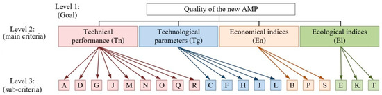
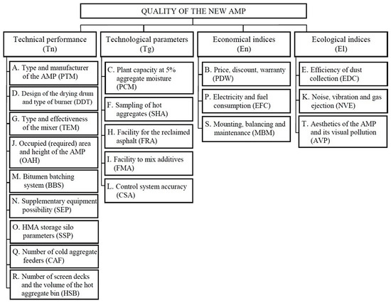
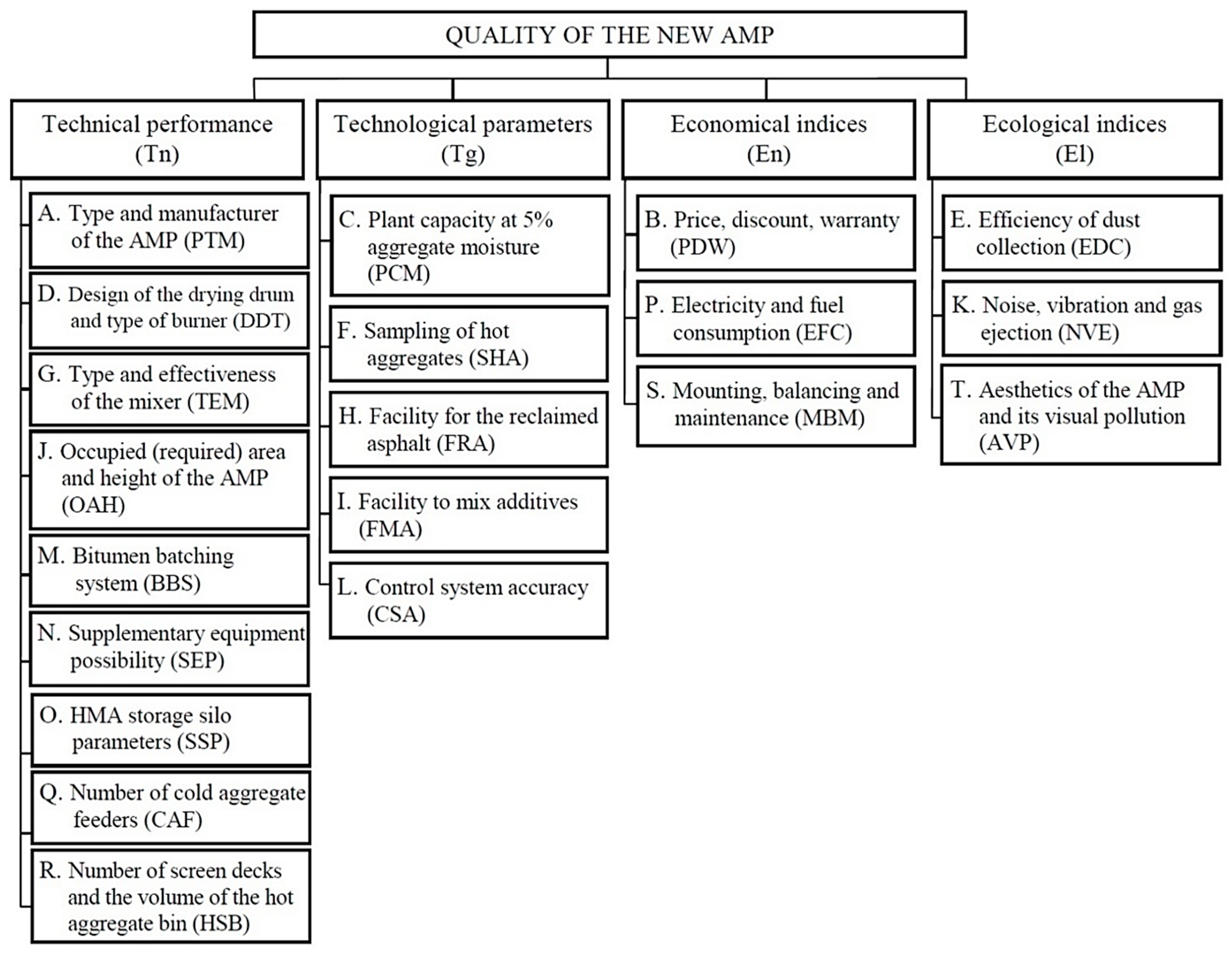
To assess the importance of the 20 quality criteria for AMPs, they were divided into four groups, forming a hierarchical structure (Figure 4). Based on the definitions of the criteria, four main quality categories were identified: technical performance, technological parameters, economic, and ecological indices. Each main criterion (Level 2) comprises 3 to 9 sub-criteria (Level 3).

Figure 4. The hierarchy model of the quality criteria of the AMP.

The more sub-criteria a main criterion contains, the lower their relative local weights are. To eliminate the effect of the different number of the sub-criteria in the main criterion on global weights ${\omega }_{i.g}$, the weight ${\omega }_c$ of the main criterion must be multiplied by the local weight ${\omega }_{i.c}$ of the sub-criterion, and the obtained result must be multiplied by the number of the sub-criteria in the main criterion $m_c$:

$${\omega }_{i.g}={\omega }_c·{\omega }_{i.c}·m_{\mathrm{c}}.$$

(16)

The subjective normalized global weight ${\tilde{\omega }}_{i.g}$ of the i-th sub-criterion is calculated while using the following formula:

$${\tilde{\omega }}_{ i.g}={\displaystyle \frac{{\omega }_{i.g}}{{\displaystyle \sum _{i=1}^m{\omega }_{i.g}}}}.$$

(17)

The experts initially ranked the main criteria and filled in the matrix indicating their importance $\mathbf{A}={\left[a_{ij}\right]}_{4\times 4}$. Then, they evaluated the importance of the sub-criteria, making each main criterion by filling in four more pairwise comparison matrices.

Once the weights of the AMP sub-criteria are established, they may fall into several groups of sub-criteria (main criteria), so that each of the groups would contain only the sub-criteria, which have the same attributes. As noted earlier, the twenty sub-criteria were divided into four main criteria, forming a three-level hierarchical model for the AMP quality system (Figure 3). The first main criterion consists of 9 sub-criteria for the technical performance; the second main criterion includes 5 sub-criteria for the technological parameters; the third main criterion covers 3 sub-criteria for the economical indices; and the fourth main criterion contains 3 sub-criteria for the ecological indices. The weight of each main criterion must be determined. Once these weights are established, a new simplified model of the AMP quality system can be developed, enabling road construction companies to analyze AMPs while considering generalized units of the properties.

The Inverse Hierarchy for Assessment Main Criteria Importance (IHAMCI) method allows for the calculation of the weights of the main criteria while taking into account the global weights of the sub-criteria. To apply this approach, the following steps should be followed:

STEP 1: The subjective global weights ${\omega }_i$ of the sub-criteria of the investigated object (AMP), which were calculated while applying the known approaches (AHP, ARTIW-L, etc.) or expressed through the arithmetic mean of several methods, are provided in the column in random order. The total sum should be equal to ${\sum }_{i=1}^m{\omega }_i=1$, $\left(i=1, 2,\dots ,m\right)$.

STEP 2: While taking into account the common attributes, the sub-criteria (their number $m$) is divided into the separate groups of the sub-criteria (main criteria). The main criteria $k$ $\left(c=1, 2, \dots ,k\right)$ are obtained from the sub-criteria $m$. Every c-th main criterion is made of the sub-criteria $m_c$ $\left(i=1, 2, \dots , m_c,{\sum }_{c=1}^k{m}_c=m\right)$.

STEP 3: The global weights ${\omega }_i$ of the sub-criteria $m_c$ making every c-th main criterion are determined:

$${\omega }_c={\displaystyle \sum _{i=1}^{m_c}{\omega }_i<1}.$$

(18)

STEP 4: The global weights of (number of these weights is $k$) of the sub-criteria for every c-th main criterion $\left(c=1, 2,\dots ,k\right)$ are normalized:

$${\omega }_g={\displaystyle \frac{{\omega }_i}{{\omega }_c}}={\displaystyle \frac{{\omega }_i}{{\displaystyle \sum _{i=1}^{m_c}{\omega }_i}}}=1.0000.$$

(19)

STEP 5: The average of the weights ${\overline{\omega }}_c$ of the normalized sub-criteria for every c-th main criterion is calculated as follows:

$${\overline{\omega }}_c={\displaystyle \frac{{\omega }_c}{m_c}},$$

(20)

where $m_c$ represents the number of the sub-criteria making the main criterion.

If all main criteria of the hierarchical structure were equal—that is, if they each consisted of the same number of sub-criteria—the most important criterion would be the one with the highest total local weight. However, in the common case, the main criteria that form the hierarchical structure often contain different numbers of sub-criteria that must be evaluated.

STEP 6: The weights ${\overline{\omega }}_c$ of each c-th main criterion (expressed by the number $k$), showing the final result of the calculations are normalized:

$${\tilde{\omega }}_c={\displaystyle \frac{{\overline{\omega }}_c}{{\displaystyle \sum _{c=1}^k{\overline{\omega }}_c}}}.$$

(21)

The sum of all the normalized weights of the main criteria $k$ should be ${\sum }_{c=1}^k{\tilde{\omega }}_c=1.000$ and can be expressed in a form of percentage, i.e., be equal to 100%.

3. Results and Discussion

3.1. Weights of the AMP Properties Determined Using the ARTIW-L and ARTW-N Methods

The ARTIW-L and ARTIW-N methods were initially applied in order to calculate rank means ${\overline{R}}_i$ of 20 AMP quality criteria while using Formula (2). The average values of the criterion ranking and their priorities are presented in Table 1.

Table 1. AMP properties’ significance ranks, relative weights, and priority, calculated using the ARTIW-L and ARTIW-N methods.

Indicator	Asphalt Mixing Plant Priority (Quality Criterion), i = 1, 2, …, m																				Total
	A	B	C	D	E	F	G	H	I	J	K	L	M	N	O	P	Q	R	S	T
$\sum _{\mathit{e}=1}^{\mathit{n}}{\mathit{R}}_{\mathit{i}\mathit{e}}$	204	196	154	200	257	439	143	305	321	496	515	190	265	296	368	323	298	280	481	569	6300
$\overline{{\mathit{R}}_{\mathit{i}}}=\sum _{\mathit{e}=1}^{\mathit{n}}{\displaystyle \frac{{\mathit{R}}_{\mathit{i}\mathit{e}}}{\mathit{n}}}$	6.80	6.53	5.13	6.67	8.57	14.63	4.77	10.17	10.70	16.53	17.17	6.33	8.83	9.87	12.27	10.77	9.93	9.33	16.03	18.97	210.00
$\sum _{\mathit{e}=1}^{\mathit{n}}{\mathit{R}}_{\mathit{i}\mathit{e}}-\overline{\mathit{R}}$	−111	−119	−161	−115	−58	124	−172	−10	6	181	200	−125	−50	−19	53	8	−17	−35	166	254	0
${\left[\sum _{\mathit{e}=1}^{\mathit{n}}{\mathit{R}}_{\mathit{i}\mathit{e}}-\overline{{\mathit{R}}_{\mathit{i}}}\right]}^2$	12,321	14,161	25,921	13,225	3364	15,376	29,584	100	36	32,761	40,000	15,625	2500	361	2809	64	289	1225	27,556	64,516	301,794
ARTIW-L:
${\mathit{\omega }}_{\mathit{i}}^{\mathit{A}\mathit{R}\mathit{T}\mathit{I}\mathit{W}-\mathit{L}}$	0.0676	0.0689	0.0756	0.0682	0.0592	0.0303	0.0773	0.0516	0.0490	0.0213	0.0182	0.0698	0.0580	0.0530	0.0416	0.0487	0.0527	0.0556	0.0237	0.0097	1.000
Priority	6	4	2	5	7	16	1	12	13	18	19	3	8	10	15	14	11	9	17	20	210
ARTIW-N:
ui	0.7015	0.7305	0.9298	0.7151	0.5566	0.3260	1	0.4690	0.4458	0.2886	0.2778	0.7536	0.5402	0.4833	0.3888	0.4429	0.4804	0.55112	0.2976	0.2514	10.5901
${\mathit{\omega }}_{\mathit{i}}^{\mathit{A}\mathit{R}\mathit{T}\mathit{I}\mathit{W}-\mathit{N}}$	0.0662	0.0690	0.0878	0.0675	0.0526	0.0308	0.0944	0.0443	0.0421	0.0273	0.0262	0.0712	0.0510	0.456	0.0367	0.0418	0.4854	0.0483	0.0281	0.0237	1.0000
Priority	6	4	2	5	7	16	1	12	13	18	19	3	8	10	15	14	11	9	17	20	210

Consistency in the opinions expressed by the thirty-expert group as a prerequisite for using ${\overline{R}}_i$ as a reliable result of problem solving has been calculated while using Formula (7):

$$W={\displaystyle \frac{12S}{n^2\left(m^3-m\right)}}={\displaystyle \frac{12·301 794}{{30}^2\left({20}^3-20\right)}}=0.50425.$$

While applying Formula (8), the concordance coefficient $W$ has been used in order to calculate the Chi-Square distribution ${\chi }^2$:

$${\chi }^2=Wn\left(m-1\right)=0.50425·30\left(20-1\right)=287.42.$$

While considering the exact level of significance $\alpha =0.01$ and a degree of freedom $\nu =m-1=20-1=19$, from the distribution ${\chi }_{v,\alpha }^2$, the critical value of this statistical indicator is found to be ${\chi }_{19,0.01}^2=36.19$. The calculated value of ${\chi }^2$ is almost 7.9 times higher than the critical value of ${\chi }_{v,\alpha }^2$, which allows us to assume that the opinions of thirty experts on the importance of AMP quality criteria are consistent and their rank ${\overline{R}}_i$ can be used for calculating the weights of these criteria.

In addition, it has been verified whether the estimated values of the concordance coefficient $W=0.504$ are a reliable indicator of consistency in expert opinions. For this purpose, its minimum value has been set:

$$W_{\min }={\displaystyle \frac{{\chi }_{v, \alpha }^2}{n\left(m-1\right)}}={\displaystyle \frac{36.19}{30\left(20-1\right)}}=0.0635.$$

It can be seen that the calculated value $W=0.504$ is about eight times higher than the minimum value of the concordance coefficient $W_{\mathrm{m}\mathrm{i}\mathrm{n}}=0.0635$, which allows us to use the ranked means ${\overline{R}}_i$ of the expert group in order to define the weights of these criteria.

The ARTIW-L method was also used while calculating the normalized weights ${\omega }_i$ of all the quality criteria of the AMP. According to the Formula (1), the global weight of the first criterion (A) is equal to

$${\omega }_A={\displaystyle \frac{\left(m+1\right)-{\overline{R}}_i}{{\displaystyle \sum _{i=1}^m{\overline{R}}_i}}}={\displaystyle \frac{\left(20+1\right)-6.800}{210}}=0.06762.$$

The global weights and priorities of all 20 quality criteria for the new AMP were calculated using the ARTIW-L and ARTW-N methods and are presented in Table 1. The difference between the most important criterion (G) and least important criterion (T) is 0.0676 and 0.0707. The relative weight of the most important criterion is approximately eight times greater than the weight of the least important criterion calculated using the ARTIW-L method. The ratio, calculated using the ARTIW-N method, is equal to 4.

3.2. Weights of the Non-Hierarchical Structured AMP Criteria Determined Using the AHP Method

Firstly, while applying the AHP method, the pairwise comparison matrix of criteria was completed (Table 2). The consistency ratio $C.R.$ of the pairwise comparison matrix is 0.0278, which is below the threshold of 0.1. Therefore, the eigenvector ${\omega }_i^{AHP}$, calculated using Formula (11), can be used to determine the importance of the AMP quality criteria. The normalized weights and ranks of these criteria, established using the AHP method without creating a hierarchical structure or dividing the criteria into groups and sub-criteria, are presented in Table 2.

Table 2. The pairwise comparison matrix of the AMP quality criteria (no hierarchical structure).

Criteria		Quality Criteria of the AMP j = 1, 2, …, m																				Global Weight ${\mathit{\omega }}_{\mathit{i}}^{\mathit{A}\mathit{H}\mathit{P}}$(Priority)
		A	B	C	D	E	F	G	H	I	J	K	L	M	N	O	P	Q	R	S	T
Quality criteria of the AMP i = 1, 2, …, m	A	1	1/2	1/2	1	2	5	1/3	3	5	7	7	1/2	2	2	5	4	3	2	6	7	0.0732 (5)
	B	2	1	1/2	2	2	7	1/3	5	5	7	8	1/2	3	4	6	6	4	3	7	8	0.0975 (4)
	C	2	2	1	3	3	7	1/2	5	6	7	8	1	4	5	6	6	5	4	7	9	0.1228 (3)
	D	1	1/2	1/3	1	1	5	1/4	3	4	6	7	1/3	1	2	5	4	3	2	5	7	0.0629 (6)
	E	1/2	1/2	1/3	1	1	5	1/4	3	4	5	6	1/3	1	2	5	4	3	2	5	6	0.0628 (7)
	F	1/5	1/7	1/7	1/5	1/5	1	1/8	1/3	1/2	2	2	1/7	1/5	1/4	1	1/2	1/3	1/4	1	3	0.0135 (16)
	G	3	3	2	4	4	8	1	6	7	9	9	2	5	6	7	7	6	5	8	9	0.1622 (1)
	H	1/3	1/5	1/5	1/3	1/3	3	1/6	1	1	3	4	1/5	1/3	1/2	2	2	1	1/2	3	4	0.0262 (12)
	I	1/5	1/5	1/6	1/4	1/4	2	1/7	1	1	3	4	1/6	1/3	1/2	2	1	1/2	1/3	2	4	0.0212 (13)
	J	1/7	1/7	1/7	1/6	1/5	1/2	1/9	1/3	1/3	1	1	1/7	1/5	1/4	1/2	1/2	1/4	1/4	1	2	0.0107 (18)
	K	1/7	1/8	1/8	1/7	1/6	1/2	1/9	1/4	1/4	1	1	1/8	1/6	1/5	1/3	1/3	1/4	1/5	1/2	2	0.0091 (19)
	L	2	2	1	3	3	7	1/2	5	6	7	8	1	4	5	7	6	5	4	7	8	0.1230 (2)
	M	1/2	1/3	1/4	1	1	5	1/5	3	3	5	6	1/4	1	2	4	4	2	1	5	6	0.0515 (8)
	N	1/2	1/4	1/5	1/2	1/2	4	1/6	2	2	4	5	1/5	1/2	1	3	3	1	1	4	5	0.0366 (10)
	O	1/5	1/6	1/6	1/5	1/5	1	1/7	1/2	1/2	2	3	1/7	1/4	1/3	1	1	1/3	1/3	2	3	0.0160 (15)
	P	1/4	1/6	1/6	1/4	1/4	2	1/7	1/2	1	2	3	1/6	1/4	1/3	1	1	1/2	1/3	2	4	0.0185 (14)
	Q	1/3	1/4	1/5	1/3	1/3	3	1/6	1	2	4	4	1/5	1/2	1	3	2	1	1/2	3	5	0.0303 (11)
	R	1/2	1/3	1/4	1/2	1/2	4	1/5	2	3	4	5	1/4	1	1	3	3	2	1	4	5	0.0420 (9)
	S	1/6	1/7	1/7	1/5	1/5	1	1/8	1/3	1/2	1	2	1/7	1/5	1/4	1/2	1/2	1/3	1/4	1	2	0.0122 (17)
	T	1/7	1/8	1/9	1/7	1/6	1/3	1/9	1/4	1/4	1/2	1/2	1/8	1/6	1/5	1/3	1/4	1/5	1/5	1/2	1	0.0077 (20)

${\lambda }_{\mathrm{m}\mathrm{a}\mathrm{x}}=20.94$, $C.I.=0.0096,R.I.=1.782$, $C.R.=0.0278.$

The difference between the weights of the most important (G) and least important (T) criterion is 0.1622. This means that G is approximately 21 times more significant than T criterion. Correctly filling in a matrix $\mathbf{A}={\left|a_{ij}\right|}_{20\times 20}$ of this size so that C. R. is less than 0.1 is challenging; however, for a skilled expert familiar with the principles of the AHP method, it is achievable.

3.3. Weights of the Hierarchically Structured AMP Criteria Determined Using the AHP Method

In this case, all AMP quality criteria were organized into a hierarchical structure (Figure 2 and Figure 4). The first main criterion of the technical performance (Tn) consists of nine sub-criteria, the second group of the technological parameters (Tg) is made of five sub-criteria, the third group of the criteria covers three economic sub-criteria (En), and the fourth group of the criteria is made of three ecological sub-criteria (El). The weights of the hierarchically structured criteria were set at two stages. Initially, the importance of the main criteria for the quality of the new AMP was evaluated by completing the pairwise comparison matrix (Table 3).

Table 3. The pairwise comparison matrix of the AMP quality main criteria (hierarchically structured).

Main Criterion	Tn	Tg	En	El	$\mathbf{Weight} {\mathit{\omega }}_{\mathit{c}}$
Tn	1	1/3	3	6	0.2745
Tg	3	1	5	7	0.5615
En	1/3	1/5	1	2	0.1060
El	1/6	1/7	1/2	1	0.0580

${\lambda }_{\mathrm{m}\mathrm{a}\mathrm{x}}=4.08606$, $C.I.=0.02869,R.I.=0.90$, $C.R.=0.0319.$

The results of the research show that experts find the technological parameters of the AMP the most important $\left({\omega }_{Tg}=0.561\right)$. The technical performance takes the second position $\left({\omega }_{Tn}=0.275\right)$, the economical indices go to the third $\left({\omega }_{En}=0.106\right)$, and the ecological indices occupy the fourth position $\left({\omega }_{El}=0.058\right)$. The matrix is consistent as the $C.R.=0.0319<0.1$.

During the second stage, the pairwise comparison matrices of all sub-criteria, while considering all four groups of criteria, were completed separately. The pairwise comparison matrix of the technical performance (Table 4) and the calculated eigenvector values ${\omega }_{i.c}$ can be considered as reliable and further used for determining their relative importance, because $C.R.=0.0345<0.1$. The pairwise comparison matrix of the technological parameters together with the calculated eigenvector values ${\omega }_{i.c}$ and values of the consistency ratio $R.I.$, are provided in Table 5. The pairwise comparison matrix of the economical indices $\left(C.R. =0.0032<0.1\right)$ is shown in Table 6 and the pairwise comparison matrix of the ecological indices $\left(C.R. =0.107>0.1\right)$ is shown in Table 7.

Table 4. The pairwise comparison matrix of the technical performance (Tn) of the new AMP.

Tn	A	D	G	J	M	N	O	Q	R	$\mathbf{Local} \mathbf{Weight} {\mathit{\omega }}_{\mathit{i}.\mathit{T}\mathit{n}}$
A	1	1/2	1/3	7	2	4	6	5	3	0.1570
D	2	1	1/2	8	3	5	7	6	4	0.2235
G	3	2	1	9	4	6	8	7	5	0.3081
J	1/7	1/8	1/9	1	1/6	1/4	1/2	1/3	1/5	0.0179
M	1/2	1/3	1/4	6	1	3	5	4	2	0.1084
N	1/4	1/5	1/6	4	1/3	1	3	2	1/2	0.0509
O	1/6	1/7	1/8	2	1/5	1/3	1	1/2	1/4	0.0247
Q	1/5	1/6	1/7	3	1/4	1/2	2	1	1/3	0.0352
R	1/3	1/4	1/5	5	1/2	2	4	3	1	0.0743

${\lambda }_{\mathrm{m}\mathrm{a}\mathrm{x}}=9.40046$, $C.I.=0.0506,R.I.=1.45$, $C.R.=0.0345.$

Table 5. The pairwise comparison matrix of the technological parameters (Tg) of the new AMP.

Tg	C	F	H	I	L	$\mathbf{Local} \mathbf{Weight} {\mathit{\omega }}_{\mathit{i}.\mathit{T}\mathit{g}}$
C	1	7	3	5	2	0.4216
F	1/7	1	1/4	1/2	1/6	0.0452
H	1/3	4	1	3	1/3	0.1533
I	1/5	2	1/3	1	1/5	0.0701
L	1/2	6	3	8	1	0.3098

${\lambda }_{\mathrm{m}\mathrm{a}\mathrm{x}}=5.1318$, $C.I.=0.03295,R.I.=1.12$, $C.R.=0.0294.$

Table 6. The pairwise comparison matrix of the economical indices (En) of the new AMP.

En	B	P	S	$\mathbf{Local} \mathbf{Weight} {\mathit{\omega }}_{\mathit{i}.\mathit{E}\mathit{n}}$
B	1	3	5	0.6483
P	1/3	1	2	0.2297
S	1/5	1/2	1	0.1220

${\lambda }_{\mathrm{m}\mathrm{a}\mathrm{x}}=3.0037$, $C.I.=0.00185,R.I.=0.58$, $C.R.=0.0032.$

Table 7. The pairwise comparison matrix of the ecological indices (El) of the new AMP.

El	E	K	T	$\mathbf{Local} \mathbf{Weight} {\mathit{\omega }}_{\mathit{i}.\mathit{E}\mathit{l}}$
E	1	4	7	0.6871
K	1/4	1	5	0.2437
T	1/7	1/5	1	0.0692

${\lambda }_{\mathrm{m}\mathrm{a}\mathrm{x}}=3.1237$, $C.I.=0.0619,R.I.=0.58$, $C.R.=0.1066.$

Taking into account the proposed hierarchical structure (Figure 2 and Figure 4), the weights of the main criteria for the second level and the weights of the sub-criteria for the third level have been used to calculate the normalized global weights ${\omega }_{i.g.}^{AHP}$ of the AMP quality criteria (Table 8). The normalized weights of the AMP quality sub-criteria have been determined while employing three approaches, thus the arithmetic means of these weights are calculated:

$$\overline{{\omega }_i}={\displaystyle \frac{{\omega }_i^{ARTIW-L}+{\omega }_i^{ARTIW-N}+{\omega }_i^{AHP}+{\omega }_{ig}^{AHP}}{4}}$$

(22)

where ${\omega }_i^{ARTIW-L}$ and ${\omega }_i^{ARTIW-N}$ represent the weight of the i-th AMP quality sub-criterion determined while applying the ARTIW-L and ARTIW-N methods (Table 1), ${\omega }_i^{AHP}$ represents the weight of the i-th AMP quality sub-criterion determined while applying the AHP method, when there was no hierarchical structure (Table 2), and ${\omega }_{ig}^{AHP}$ represents the global weight of the i-th AMP quality sub-criterion determined while applying the AHP method under the hierarchically structured AHP properties (Table 8).

Table 8. Quality criteria of the new AMP while considering local and global weights.

Level 1	Level 2		Level 3
Goal	Main Criterion	Weight of Main Criterion ${\mathit{\omega }}_{\mathit{c}}$ and the Number of Sub-Criteria ${\mathit{m}}_{\mathit{c}}$	Sub-Criterion	Local Weights ${\mathit{\omega }}_{\mathit{i}.\mathit{c}}$	Global Weights ${\mathit{\omega }}_{\mathit{i}.\mathit{g}}$	Normalized Global Weight ${\mathit{\omega }}_{\mathit{i}.\mathit{g}.}^{\mathit{A}\mathit{H}\mathit{P}}$ (Priority)
Quality of the new AMP	Technical performances	${\omega }_{Tn}=$0.2745 $(m_{Tn}$ = 9)	A	0.1570	0.3879	0.0672 (6)
			D	0.2235	0.5522	0.0957 (4)
			G	0.3081	0.7612	0.1319 (3)
			J	0.0179	0.0442	0.0077 (17)
			M	0.1084	0.2678	0.0464 (7)
			N	0.0509	0.1257	0.0218 (12)
			O	0.0247	0.0610	0.0106 (16)
			Q	0.0352	0.0870	0.0151 (14)
			R	0.0743	0.1836	0.0318 (10)
	Technological parameters	${\omega }_{Tg}= 0.5615$ $(m_{Tg}$ = 5)	C	0.4216	1.1836	0.2051 (1)
			F	0.0452	0.1269	0.0220 (11)
			H	0.1533	0.4304	0.0746 (5)
			I	0.0701	0.1968	0.0341 (9)
			L	0.3098	0.8698	0.1507 (2)
	Economical indices	${\omega }_{En}= 0.1060$ $(m_{En}$ = 3)	B	0.6483	0.2062	0.0357 (8)
			P	0.2297	0.0730	0.0127 (15)
			S	0.1220	0.0388	0.0067 (19)
	Ecological indices	${\omega }_{El}=$0.0580 $(m_{El}$ = 3)	E	0.6871	0.1196	0.0207 (13)
			K	0.2437	0.0424	0.0074 (18)
			T	0.0692	0.0120	0.0021 (20)
Total	–	1.0000	–	4.0000	5.7701	1.0000 –

3.4. The Average Weight of Criteria

While considering the weights ${\omega }_i^{ARTIW-L}$, ${\omega }_i^{ARTIW-N}$, ${\omega }_i^{AHP}$ and ${\omega }_{i.g.}^{AHP}$ of the 20 AMP quality criteria (Table 1, Table 2 and Table 8), based on Formula (22), the arithmetic means ${\overline{\omega }}_i$ of the weights of each criterion have been calculated. Respectively, these arithmetic means ${\overline{\omega }}_i$ can be considered as the result of the solved problem, i.e., the arithmetic means ${\overline{\omega }}_i$ determine the significance of the criteria, that being which of those criteria are the most important for the potential buyers of the AMPs (Table 9). The application of three MCDM methods allowed for increasing the reliability of the achieved solution. If all the criteria for the AMP were equally important, the weight of each of those would be equal to 0.05 or 5.00%, i.e., to the average of the normalized weights.

Table 9. The weights of the new AMP quality criteria groups (main criteria) determined while applying the IHAMCI method.

AMP Quality Sub-Criteria	Average Global Weight of Sub- Criteria ${\overline{\mathit{\omega }}}_{\mathit{i}}$	Global Rank	Description of the Main Criterion and Its Size ${\mathit{m}}_{\mathit{c}}$	Sub-Criteria Composed Main Criterion	Average Global Weight of Sub-Criteria ${\overline{\mathit{\omega }}}_{\mathit{i}}$	The Sum of the Average Global Weight in the Main Criterion ${\displaystyle \sum _{\mathit{i}=1}^{{\mathit{m}}_{\mathit{c}}}{\mathit{\omega }}_{\mathit{i}}={\mathit{\omega }}_{\mathit{c}}}$	Average Weight of the Sub-Criteria for the Main Criterion ${\overline{\mathit{\omega }}}_{\mathit{c}}=\frac{{\mathit{\omega }}_{\mathit{c}}}{{\mathit{m}}_{\mathit{c}}}$	Normalized Average Weight of the Main Criterion $\frac{{\overline{\mathit{\omega }}}_{\mathit{c}}}{{\sum }_{\mathit{c}=1}^{\mathit{k}}{\overline{\mathit{\omega }}}_{\mathit{c}}}$
A	0.0685	5	Technical performances (Tn) mTn = 9	A	0.0685	0.4729	0.4729 ÷ 9 = 0.0525	${\displaystyle \frac{0.0525}{0.1733}}=0.2864$
B	0.0678	6		D	0.0736
C	0.1228	1		G	0.1165
D	0.0736	4		J	0.0168
E	0.0488	9		M	0.0517
F	0.0241	16		N	0.0393
G	0.1165	2		O	0.0262
H	0.0492	8		Q	0.0359
I	0.0366	12		R	0.0444
J	0.0168	18	Technological parameters (Tg) mTg = 5	C	0.1228	0.3364	0.3364 ÷ 5 = 0.0673	${\displaystyle \frac{0.0673}{0.1833}}=0.3672$
K	0.0152	19		F	0.0241
L	0.1037	3		H	0.0492
M	0.0517	7		I	0.0366
N	0.0393	11		L	0.1037
O	0.0262	15	Economical indices (En) mEn = 3	B	0.0678	0.1159	0.1159 ÷ 3 = 0.0386	${\displaystyle \frac{0.0386}{0.1833}}=0.2106$
P	0.0304	14		P	0.0304
Q	0.0359	13		S	0.0177
R	0.0444	10	Ecological indices (El) mEl = 3	E	0.0488	0.0748	0.0748 ÷ 3 = 0.0249	${\displaystyle \frac{0.0249}{0.1833}}=0.1358$
S	0.0177	17		K	0.0152
T	0.0108	20		T	0.0108
Total	1.0000	210	–	–	1.0000	1.0000	0.1833	1.0000

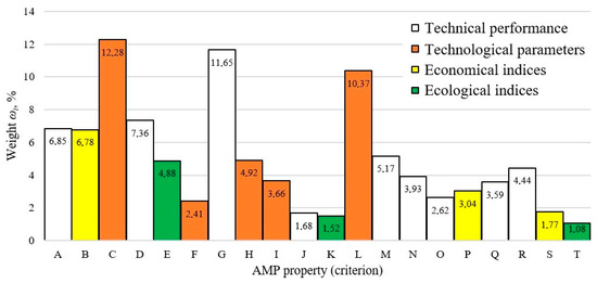
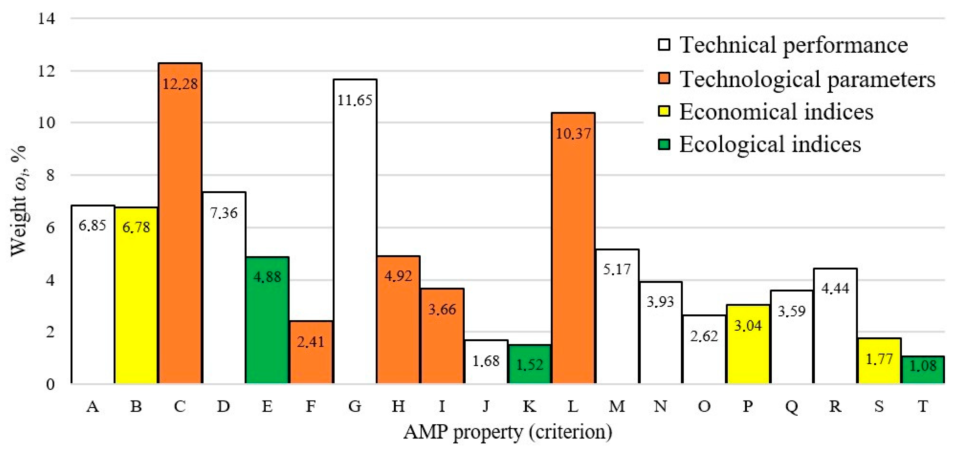
The obtained results (weights of the quality criteria of the AMP) are also presented in Figure 5. From the figure, it can be seen that the weight of the most important criterion (Plant capacity at 5% aggregate moisture) is ${\overline{\omega }}_C=12.28\%$. Respectively, the value of this weight is 11.4 times higher than the weight of the least important criterion (Esthetics of the AMP and its visual pollution), ${\overline{\omega }}_T=1.08\%$. Such a huge difference between the importance of the AMP quality criteria indicates that the potential buyers of the AMP unit realize the varying impact of individual criteria and are almost of the same opinion. They are well aware of the AMP properties determining the choice of the new AMP.

Figure 5. The percentage weight and ranking of quality criteria of the AMP.

However, it can be noted that the obtained results reveal a significant difference between the opinions of experts (AMP buyers) and those most commonly discussed in the research literature. While researchers frequently focus on AMP emissions and energy consumption, potential buyers place greater importance on the technological parameters of the (${\omega }_{Tg}=0.561$) and tend to undervalue ecological indices (${\omega }_{El}=0.058$). Criteria K and E, which are directly related to the GHG emissions, were ranked near the bottom (${\overline{\omega }}_K=1.52\%,{\overline{\omega }}_E=4.88\%$). These results indicate that emissions generated by AMPs are not taken seriously by users and buyers, highlighting the need for actions to reverse this trend.

3.5. Weights of the AMP Main Criteria Determined While Applying the IHAMCI Method

The sequence of the calculations and the results, obtained while applying the IHAMCI method, are presented in Table 9.

Respectively, while applying Formula (21), the following values of the normalized weights ${\tilde{\omega }}_C$ of each main criterion are calculated: Tn (0.2864); Tg (0.3672); En (0.2106); El (0.1358).

From Table 9 it can be seen that the results, obtained using the IHAMCI method, are relatively similar to those obtained with the AHP method for the hierarchically structured criteria (Table 3). Therefore, it can be stated that the IHAMCI method provides reliable results for ranking the main criteria while taking into account the classified sub-criteria.

3.6. The Relationship Between the Weights of the Sub-Criteria Determined Applying Different Methods

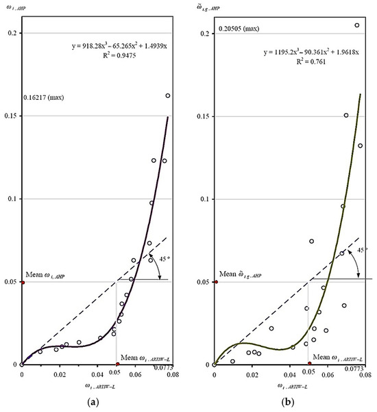
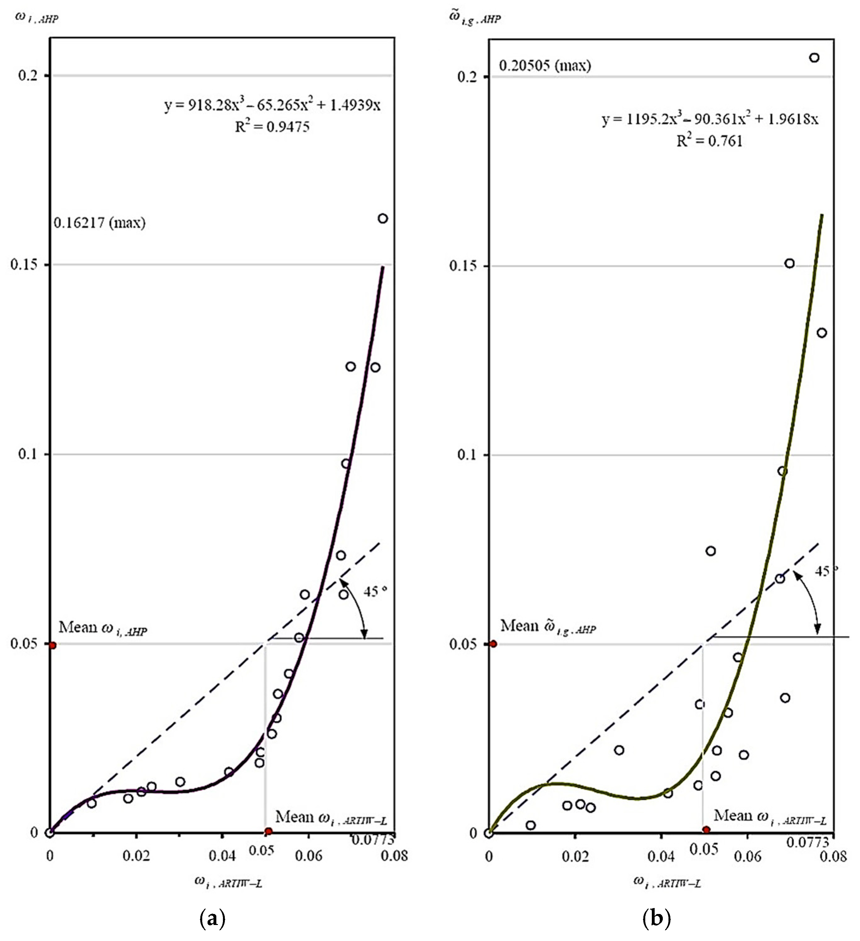
This sub-section analyzes the differences between the subjective normalized weights of AMP quality criteria determined using different methods. Such a comparison is important because there is limited information on which MCDM methods provide the most accurate determination of criterion importance. Analyzing the relationships between the weights of sub-criteria calculated with different methods reveals the “sensitivity” of these methods. It is important to note that the weights determined by different MCDM methods should be strongly correlated, functionally dependent, and follow the same upward trend. The form of this relationship is represented by a regression equation, and the strength of relationship is expressed by the coefficient of determination ${\mathrm{R}}^2$ (Figure 6).

Figure 6. The relationship between the weights of 20 AMP quality criteria, determined while applying different MCDM methods: (a) ARTIW–L and AHP with no hierarchy, (b) hierarchically structured quality criteria for ARTIW–L and AHP.

In order to determine the relationship between the weights of the AMP quality sub-criteria, the third-order regression equation has been selected:

$$y=A{x}^3+B{x}^2+Cx,$$

(23)

where $A$, $B$, and $C$ represent the coefficients of the regression equation, $x$ represents the weights of the AMP quality sub-criteria, determined while applying the ARTIW–L method $\left({\omega }_i^{ARTIW-L}\right)$, and $y$ represents the weights of the AMP quality sub-criteria, determined while applying the AHP method (without and with hierarchical structure, ${\omega }_i^{AHP}$ and ${\omega }_{i.g.}^{AHP}$).

The correlation–regression analysis of the weights of the 20 AMP quality sub-criteria, determined while using different MCDM methods, shows that the relationship between the weights has the same tendency (Figure 6). According to a curvilinear dependence, an increase in the weights of the sub-criteria for values ${\omega }_i^{ARTIW-L}$ has been identified while applying the ARTIW–L method and has resulted in a rising number of the weights determined with reference to the AHP method when sub-criteria were not hierarchically structured ${\omega }_{i, AHP}$ and when sub-criteria were hierarchically structured ${\omega }_i^{AHP}$. However, the lowest dispersion of the normalized weights of AMP quality sub-criteria was noticed while using the ARTIW–L method. The difference between the maximum weight (${\omega }_{i.\mathrm{m}\mathrm{a}\mathrm{x}}^{ARTIW-L}=0.0773$) and the minimum weight (${\omega }_{i.\mathrm{m}\mathrm{i}\mathrm{n}}^{ARTIW-L}=0.0097$) was 0.0676. The difference in the maximum weight (${\omega }_{i.\mathrm{m}\mathrm{a}\mathrm{x}}^{AHP}=0.1622$) and the minimum weight (${\omega }_{i.\mathrm{m}\mathrm{i}\mathrm{n}}^{AHP}=0.0077$) of the AMP quality sub-criteria with no hierarchy, determined while using the AHP method, is 0.1544, i.e., the difference is approximately 2.3 times higher than difference in the weights calculated while applying the ARTIW–L method. The difference between the maximum value of the global weights (${\omega }_{i.g.\mathrm{m}\mathrm{a}\mathrm{x}}^{AHP}=0.2020$) and minimum value (${\omega }_{i.g.\mathrm{m}\mathrm{i}\mathrm{n}}^{AHP}=0.0021$) of the hierarchically structured AMP quality sub-criteria is 0.203, i.e., around 3.0 times higher than while using the ARTIW method.

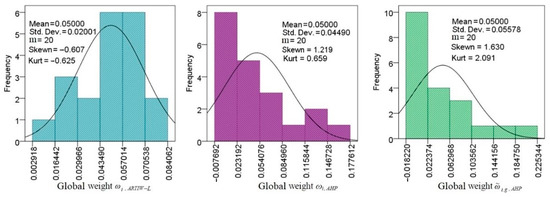
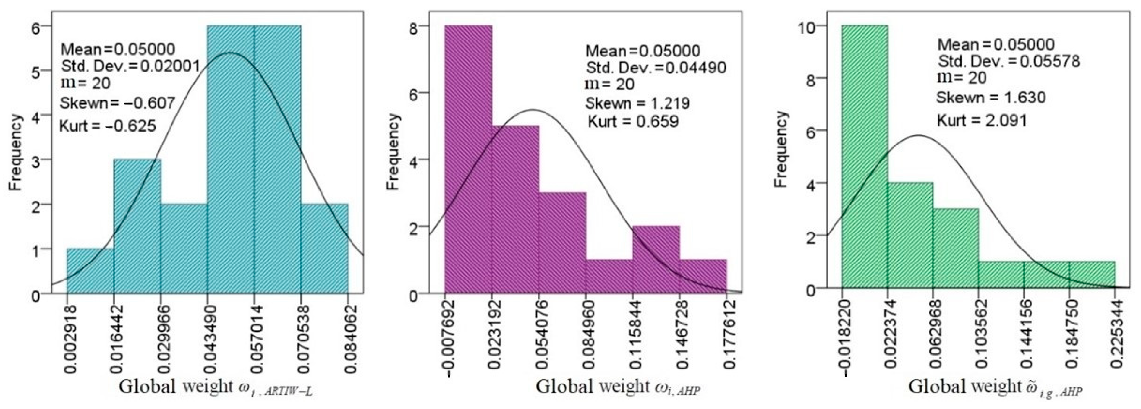
Statistical indicators (statistical mean, standard deviation, skewness, kurtosis, histograms, and theoretical curves of normal distribution) of the weights of the AMP quality sub-criteria, determined while applying different MCDM methods, are shown in Figure 7.

Figure 7. Statistical indicators of the weights of AMP quality sub-criteria determined while applying different MCDM methods.

Normal distribution of the weights of the quality sub-criteria was investigated by applying skewness and kurtosis. The values of the skewness (sk) and kurtosis (ku) calculated from the data of the sample size ($m$) were compared with their respective standard deviations s_sk and s_ku values [53]:

$$s_{sk}=\sqrt{{\displaystyle \frac{6m\left(m-1\right)}{\left(m-2\right)\left(m+1\right)\left(m+3\right)}}},$$

(24)

$$s_{ku}=\sqrt{{\displaystyle \frac{24m{\left(m-1\right)}^2}{\left(m-3\right)\left(m-2\right)\left(m+3\right)\left(m+5\right)}}},$$

(25)

where $m$ represents the size of the sample (number of the sub-criteria of AMP, $m=20$).

When $\left|sk\right|<3s_{sk}$ and $\left|ku\right|<5s_{ku}$, it can be assumed that the normality hypothesis of empirical data is proper. Otherwise, the raised hypothesis should be rejected as doubtful. It was determined that $3s_{sk}=1.54$ and $5s_{ku}=4.96$. With reference to the values of kurtosis, the normal distribution agrees with the AMP quality sub-criteria, which were determined while applying all of the described MCDM methods. However, while taking into account the values of the skewness, the distribution is not satisfied by the hierarchically structured weights ${\omega }_{i.g.}^{AHP}$ of the AMP quality sub-criteria, which were determined using the AHP method.

The equivalence of the disseminated quality sub-criteria, i.e., the significance of the differences, has been verified by calculating value $G$ of Cochran’s rule [54]:

$$G={\displaystyle \frac{s_{\omega \hspace{0.33em}\max }^2}{s_{{\omega }_{j,ARTIW–L}}^2+s_{{\omega }_{i,AHP}}^2+s_{{\tilde{\omega }}_{i.g.AHP}}^2}}.$$

(26)

Taking into account the standard deviations from the weights of the quality criteria of the AMP (Figure 7), the below value has been calculated considering the Gaussian distribution:

$$G={\displaystyle \frac{{0.05578}^2}{{0.02001}^2+{0.0449}^2+{0.05578}^2}}=0.5629.$$

While considering that the level of significance is $\alpha =0.01$, the degree of freedom is $\nu =m-1=20-1=19$ and three MCDM methods were applied, it was determined that $G_{0.01,19}=0.5358$. The result, obtained while applying Formula (26), is greater than 0.5629, which shows a significant difference between the variances of the weights of the quality criteria of the AMP, determined while applying different MCDM methods.

4. Conclusions

A literature review showed that there are no such or similar multi-criteria evaluation systems for AMP; therefore, the MCDM methods applied in this study made it possible to comprehensively assess AMP characteristics that are important to potential users of these complex technological devices. The introduced innovative system of 20 quality criteria for the evaluation of the AMPs is well-suited to comprehensively reveal the fundamental properties of this sophisticated technological equipment and to determine its suitability for use in the asphalt industry. By applying several MCDM methods (ARTIW–L, direct AHP, the hierarchical structures of the AHP), the opinions of experts with extensive knowledge of asphalt mixture production technology, AMP structure and internal processes, asphalt mixture quality, as well as economic and environmental requirements, were captured. The normalized weights of all main criteria and sub-criteria were calculated, highlighting their varying relative importance.

The position of the thirty-expert group was ranked, and arithmetic means were validly used as reliable numerical estimates to determine the importance of the AMP quality criteria. The consistency of expert opinions was confirmed by a sufficiently high value of the concordance coefficient $\left(W=0.504\right)$, which is approximately eight times higher than its minimum value $\left(W_{\mathrm{m}\mathrm{i}\mathrm{n}}=0.0635\right)$. The ARTIW–L method was applied to calculate normalized weights from the arithmetic means of the ranked AMP quality criteria, indicating the relative importance of these criteria (AMP quality indicators) and supporting decision-making when purchasing a new AMP.

The arithmetic means of the subjective normalized weights of the AMP quality indicators, determined using three MCDM methods, indicated that the key factors influencing experts’ decision to purchase a new AMP are as follows: the maximum technological capacity of the AMP (production rate) under conditions of low, medium and high moisture of aggregates (C); the type of the mixer (forced mixer and gravitation mixer); the maximum weight of one hot-mix asphalt mixture batch; minimum mixing duration (time) for the adequate homogeneity of the HMA mixture (G); the accuracy and precision of managing the technological process of producing the asphalt mixture; and the capability of a computerized control system, its operative maintenance, and the possibilities of printing data on technological parameters (L). The least important factors for experts include: the total area occupied by the AMP equipment covering the dimensions and height of the AMP (mixing tower, chimney, reclaimed dust and imported filler silo), which determines the type of the mounted crane, hoisting duty and lifting height (J); the level of noise and vibration; the intensity of the dispersion of the vapour of the bituminous binder, its additive and the gas of the dryer drum (K); the esthetics and environmental friendliness of the AMP (exterior colour combinations, graphics); and the area where it is mounted (height predominance comparing locations beside houses and parks (woods), i.e., visual pollution (T).

It was observed that the opinions of the experts differ considerably from those most commonly discussed in the research literature. While researchers pay substantial attention to emissions and energy consumption of AMPs, potential buyers place greater importance on the technological parameters of AMPs $({\omega }_{Tg}=0.561)$ and its technical performance $({\omega }_{Tn}=0.275)$. Respectively, potential buyers tend to underestimate economic indices (${\omega }_{En}=0.106$) and ecological indices (${\omega }_{El}=0.058$). These results indicate that emissions generated by the AMPs are not seriously considered between the users and buyers of the AMPs. At present, experts consider technological AMP indicators to be more important than environmental ones, despite the fact that the latter are becoming increasingly important worldwide. Over time, as environmental requirements become stricter, this ratio is likely to change. Moreover, the obtained results are most relevant to the Baltic states due to similar natural and ecological conditions. AMP designers and manufacturers can improve these devices so that their buyers obtain the maximum overall benefit.

The subjective weights of the AMP quality criteria determined using three different MCDM methods have showed the same trend in the variation in criterion importance. The strong correlation between the weights of the AMP quality criteria calculated using the ARTIW–L and AHP (no hierarchical structure) methods, as well as the ARTIW–L and AHP (hierarchically structured criteria) techniques, points to consistent expert opinions. The range between the most and least important AMP quality criteria determined using the AHP method without a hierarchical structure was approximately 2.3 times greater than the corresponding range obtained using the ARTIW–L method. An even larger difference in the range of weights—approximately 3.0 times—was observed when the AHP method with a hierarchical structure was applied.

Future research will focus on evaluating the effectiveness of increasingly stringent environmental requirements imposed on operating AMPs in recent years, as well as identifying opportunities for improvement and practical implementation methods. The impact of practical measures—such as reducing energy consumption and fuel combustion emissions, lowering the production temperature of the HMA mixture, and improving the thermal insulation efficiency of the baghouse, drum dryer, and hot storage silo—on the sustainability of the HMA production process will be assessed.

In addition, an article has already been prepared based on this study, proposing the application of tolerance limits when assessing AMP process capability indices for the number of components and their variation in the manufactured HMA data.

References

- Zapata, P.; Gambatese, J.A. Energy Consumption of Asphalt and Reinforced Concrete Pavement Materials and Construction. J. Infrastruct. Syst. 2005, 11, 9–20. [Google Scholar] [CrossRef] [Scilit]
- Yang, S.; Krayushkina, K.; Skrypchenko, O.; Ji, J.; Bieliatynskyi, A. Improvement of the Method for Increasing Roughness of Asphalt and Cement-Concrete Surfaces of Highways and Airfields. Arch. Civ. Mech. Eng. 2023, 23, 121. [Google Scholar] [CrossRef] [Scilit]
- La Placa, A.; Autelitano, F.; Neduzha, L.; Tiutkin, O.; Giuliani, F. Roles and Functions of Asphalt Sub-Ballast in the Modern Maintenance of the European Railways. Int. J. Transp. Sci. Technol. 2025, 20, 285–299. [Google Scholar] [CrossRef] [Scilit]
- Žuraulis, V.; Sivilevičius, H.; Šabanovič, E.; Ivanov, V.; Skrickij, V. Variability of Gravel Pavement Roughness: An Analysis of the Impact on Vehicle Dynamic Response and Driving Comfort. Appl. Sci. 2021, 11, 7582. [Google Scholar] [CrossRef] [Scilit]
- EAPA. Asphalt in Figures 2023; European Asphalt Pavement Association: Brussels, Belgium, 2023. [Google Scholar]
- SNS Insider. Asphalt Market Size, Share & Industry Analysis, By Product (Paving, Roofing, and Others), By Application (Roadways, Waterproofing, Recreation, and Others), and Regional Forecast, 2024–2032; SNS Insider: Pune, India, 2025. [Google Scholar]
- Wang, J.; Pan, K.; Sha, C.; Wang, Z.; Sun, Y.; Kang, Y. Carbon Emission Calculation and Uncertainty Analysis of Asphalt Concrete during the Production Stage. Constr. Build. Mater. 2024, 447, 138007. [Google Scholar] [CrossRef] [Scilit]
- Asphalt Mixing Plant Workflow 2021. Available online: https://ampsic.com/asphalt-plant-control-systems/ (accessed on 15 September 2025).
- Cheraghian, G.; Cannone Falchetto, A.; You, Z.; Chen, S.; Kim, Y.S.; Westerhoff, J.; Moon, K.H.; Wistuba, M.P. Warm Mix Asphalt Technology: An up to Date Review. J. Clean. Prod. 2020, 268, 122128. [Google Scholar] [CrossRef] [Scilit]
- Kok, B.V.; Kuloglu, N. Effects of Two-Phase Mixing Method on Mechanical Properties of Hot Mix Asphalt. Road Mater. Pavement Des. 2011, 12, 721–738. [Google Scholar] [CrossRef]
- Xie, J.; Wang, Z.; Wang, F.; Wu, S.; Chen, Z.; Yang, C. The Life Cycle Energy Consumption and Emissions of Asphalt Pavement Incorporating Basic Oxygen Furnace Slag by Comparative Study. Sustainability 2021, 13, 4540. [Google Scholar] [CrossRef] [Scilit]
- Han, Y.; Fu, J.; Zhang, Q.; Zhang, H.; Yang, F. Monitoring and Evaluation of Energy Consumption in the Whole Process of Asphalt Pavement Construction. IOP Conf. Ser. Earth Environ. Sci. 2021, 804, 042058. [Google Scholar] [CrossRef] [Scilit]
- Androjić, I.; Alduk, Z.D. Analysis of Energy Consumption in the Production of Hot Mix Asphalt (Batch Mix Plant). Can. J. Civ. Eng. 2016, 43, 1044–1051. [Google Scholar] [CrossRef] [Scilit]
- Huang, X.; Yang, J.; Fang, H.; Cai, Y.; Zhu, H.; Lv, N. Energy Consumption Analysis and Prediction of Hot Mix Asphalt. IOP Conf. Ser. Mater. Sci. Eng. 2019, 490, 032029. [Google Scholar] [CrossRef] [Scilit]
- Thives, L.P.; Ghisi, E. Asphalt Mixtures Emission and Energy Consumption: A Review. Renew. Sustain. Energy Rev. 2017, 72, 473–484. [Google Scholar] [CrossRef] [Scilit]
- Zaumanis, M.; Jansen, J.; Haritonovs, V.; Smirnovs, J. Development of Calculation Tool for Assessing the Energy Demand of Warm Mix Asphalt. Procedia-Soc. Behav. Sci. 2012, 48, 163–172. [Google Scholar] [CrossRef] [Scilit]
- Grabowski, W.; Janowski, L.; Wilanowicz, J. Problems of Energy Reduction During the Hot-Mix Asphalt Production. Balt. J. Road Bridge Eng. 2013, 8, 40–47. [Google Scholar] [CrossRef] [Scilit]
- Sukhija, M.; Saboo, N.; Pani, A. Economic and Environmental Aspects of Warm Mix Asphalt Mixtures: A Comparative Analysis. Transp. Res. Part. D Transp. Environ. 2022, 109, 103355. [Google Scholar] [CrossRef] [Scilit]
- Cimbola, Z.; Dolaček-Alduk, Z.; Dimter, S. Possibilities of Energy Savings in Hot-Mix Asphalt Production. In Proceedings of the 4th International Conference on Road and Rail Infrastructure, Šibenik, Croatia, 23–25 May 2016. [Google Scholar]
- Espinoza, M.; Campos, N.; Yang, R.; Ozer, H.; Aguiar-Moya, J.P.; Baldi, A.; Loría-Salazar, L.G.; Al-Qadi, I.L. Carbon Footprint Estimation in Road Construction: La Abundancia–Florencia Case Study. Sustainability 2019, 11, 2276. [Google Scholar] [CrossRef] [Scilit]
- Kim, B.; Lee, H.; Park, H.; Kim, H. Framework for Estimating Greenhouse Gas Emissions Due to Asphalt Pavement Construction. J. Constr. Eng. Manag. 2012, 138, 1312–1321. [Google Scholar] [CrossRef] [Scilit]
- Worford, D. Asphalt Industry Outlines Plans to Reach Net Zero Carbon Emissions by 2050. E+ELeader For Sustainable Tomorrow 2022. Available online: https://aimixgroup.com/asphalt-mixing-plant/types/ (accessed on 15 September 2025).
- Le Guen, L.; Huchet, F.; Tamagny, P. Drying and Heating Modelling of Granular Flow: Application to the Mix-Asphalt Processes. J. Appl. Fluid Mech. 2011, 4, 71–80. [Google Scholar] [CrossRef] [Scilit]
- Wang, C.; Li, Q.; Wang, K.C.P.; Sun, X.; Wang, X. Emission Reduction Performance of Modified Hot Mix Asphalt Mixtures. Adv. Mater. Sci. Eng. 2017, 2017, 2506381. [Google Scholar] [CrossRef] [Scilit]
- Santos, M.B.D.; Candido, J.; Baulé, S.D.S.; Oliveira, Y.M.M.D.; Thives, L.P. Greenhouse Gas Emissions and Energy Consumption in Asphalt Plants. Rev. Eletrônica GestãoEduc. Tecnol. Ambient. 2020, 24, e7. [Google Scholar] [CrossRef] [Scilit]
- Wang, H.; Al-Saadi, I.; Lu, P.; Jasim, A. Quantifying Greenhouse Gas Emission of Asphalt Pavement Preservation at Construction and Use Stages Using Life-Cycle Assessment. Int. J. Sustain. Transp. 2020, 14, 25–34. [Google Scholar] [CrossRef] [Scilit]
- Zhao, D. Quantitative Evaluation Method for Greenhouse Gas Emissions in Asphalt Pavement Construction Stage. IOP Conf. Ser. Earth Environ. Sci. 2020, 587, 012019. [Google Scholar] [CrossRef] [Scilit]
- Qin, X.; Sun, X. Quantitative Investigation and Decision Support of Reducing Effect of Warm Mixed Asphalt Mixture (WMA) on Emission and Energy Consumption in Highway Construction. Environ. Sci. Pollut. Res. 2022, 29, 33383–33399. [Google Scholar] [CrossRef] [Scilit]
- Rubio, M.D.C.; Moreno, F.; Martínez-Echevarría, M.J.; Martínez, G.; Vázquez, J.M. Comparative Analysis of Emissions from the Manufacture and Use of Hot and Half-Warm Mix Asphalt. J. Clean. Prod. 2013, 41, 1–6. [Google Scholar] [CrossRef] [Scilit]
- Sivilevičius, H.; Vislavičius, K.; Bražiūnas, J. Technological and Economic Design of Asphalt Mixture Composition Based On Optimization Methods. Technol. Econ. Dev. Econ. 2017, 23, 627–648. [Google Scholar] [CrossRef] [Scilit]
- Liu, Y.; You, Z.; Dai, Q.; Mills-Beale, J. Review of Advances in Understanding Impacts of Mix Composition Characteristics on Asphalt Concrete (AC) Mechanics. Int. J. Pavement Eng. 2011, 12, 385–405. [Google Scholar] [CrossRef] [Scilit]
- Vadood, M.; Johari, M.S.; Rahaei, A.R. Introducing a Simple Method to Determine Aggregate Gradation of Hot Mix Asphalt Using Image Processing. Int. J. Pavement Eng. 2014, 15, 142–150. [Google Scholar] [CrossRef] [Scilit]
- Shen, S.; Yu, H. Analysis of Aggregate Gradation and Packing for Easy Estimation of Hot-Mix-Asphalt Voids in Mineral Aggregate. J. Mater. Civ. Eng. 2011, 23, 664–672. [Google Scholar] [CrossRef] [Scilit]
- Zulkati, A.; Diew, W.Y.; Delai, D.S. Effects of Fillers on Properties of Asphalt-Concrete Mixture. J. Transp. Eng. 2012, 138, 902–910. [Google Scholar] [CrossRef] [Scilit]
- Santos, L.G.D.P.; Baptista, A.M.D.C.; Capitão, S.D. Assessment of the Use of Hot-Mix Recycled Asphalt Concrete in Plant. J. Transp. Eng. 2010, 136, 1159–1164. [Google Scholar] [CrossRef] [Scilit]
- Mogawer, W.S.; Austerman, A.J.; Bonaquist, R. Determining the Influence of Plant Type and Production Parameters on Performance of Plant-Produced Reclaimed Asphalt Pavement Mixtures. Transp. Res. Rec. J. Transp. Res. Board 2012, 2268, 71–81. [Google Scholar] [CrossRef] [Scilit]
- Sivilevicius, H.; Zavadskas, E.K.; Turskis, Z. Quality Attributes and Complex Assessment Methodology of the Asphalt Mixing Plant. Balt. J. Road Bridge Eng. 2008, 3, 161–166. [Google Scholar] [CrossRef] [Scilit]
- Sivilevičius, H.; Skrickij, V.; Skačkauskas, P. The Correlation between the Number of Asphalt Mixing Plants and the Production of Asphalt Mixtures in European Countries and the Baltic States. Appl. Sci. 2021, 11, 9375. [Google Scholar] [CrossRef] [Scilit]
- Ivanović, B.; Saha, A.; Stević, Ž.; Puška, A.; Zavadskas, E.K. Selection of Truck Mixer Concrete Pump Using Novel MEREC DNMARCOS Model. Arch. Civ. Mech. Eng. 2022, 22, 173. [Google Scholar] [CrossRef] [Scilit]
- Kendall, M.; Gibbons, J.D. Rank Correlation Methods, 5th ed.; Oxford University Press: London, UK, 1990; ISBN 0-19-520837-4. [Google Scholar]
- Zavadskas, E.K.; Podvezko, V. Integrated Determination of Objective Criteria Weights in MCDM. Int. J. Inf. Technol. Decis. Mak. 2016, 15, 267–283. [Google Scholar] [CrossRef] [Scilit]
- Sivilevičius, H.; Maskeliūnaitė, L. Assessment of the Quality of Passenger Transportation by Train Using Multiple Criteria Decision Making Methods; Lecture Notes in Intelligent Transportation and Infrastructure; Springer Nature: Cham, Switzerland, 2025; ISBN 978-3-031-85876-5. [Google Scholar]
- Sivilevičius, H. Application of Expert Evaluation Method to Determine the Importance of Operating Asphalt Mixing Plant Quality Criteria and Rank Correlation. Balt. J. Road Bridge Eng. 2011, 6, 48–58. [Google Scholar] [CrossRef] [Scilit]
- Sivilevičius, H.; Maskeliūnaitė, L. Multiple Criteria Evaluation and the Inverse Hierarchy Model for Justifying the Choice of Rail Transport Mode. Promet-Traffic Transp. 2018, 30, 57–69. [Google Scholar] [CrossRef] [Scilit]
- Saaty, T.L. The Analytic Hierarchy Process; McGraw-Hill: New York, NY, USA, 1980. [Google Scholar]
- Saaty, T.L.; Ozdemir, M.S. Why the Magic Number Seven plus or Minus Two. Math. Comput. Model. 2003, 38, 233–244. [Google Scholar] [CrossRef] [Scilit]
- Saaty, T.L. Decision Making with the Analytic Hierarchy Process. Int. J. Serv. Sci. 2008, 1, 83–98. [Google Scholar] [CrossRef] [Scilit]
- Chen, S.-L.; Pham, V.K.; Chen, J.K.C. Evaluating and Selecting the Best Outsourcing Service Country in East and Southeast Asia: An AHP Approach. J. Test. Eval. 2016, 44, 89–101. [Google Scholar] [CrossRef] [Scilit]
- Brunelli, M. Introduction to the Analytic Hierarchy Process; Springer: Berlin/Heidelberg, Germany, 2015. [Google Scholar]
- Stanujkic, D. An Extension of The Ratio System Approach of Moora Method for Group Decision-Making Based on Interval-Valued Triangular Fuzzy Numbers. Technol. Econ. Dev. Econ. 2015, 22, 122–141. [Google Scholar] [CrossRef] [Scilit]
- Liao, M.-S.; Ding, J.-F.; Liang, G.-S.; Lee, K.-L. Key Criteria for Evaluating the Green Performance of Ports. J. Test. Eval. 2016, 44, 1791–1801. [Google Scholar] [CrossRef] [Scilit]
- Taha, H.A. Operations Research: An Introduction, 9th ed.; Pearson: London, UK, 2010; ISBN 0-13-255593-X. [Google Scholar]
- Sivilevičius, H.; Bražiūnas, J.; Prentkovskis, O. Technologies and Principles of Hot Recycling and Investigation of Preheated Reclaimed Asphalt Pavement Batching Process in an Asphalt Mixing Plant. Appl. Sci. 2017, 7, 1104. [Google Scholar] [CrossRef] [Scilit]
- Snedecor, G.W.; Cochran, W.G. Statistical Methods, 7th ed.; Iowa State: Ames, IA, USA, 1980. [Google Scholar]
Disclaimer/Publisher’s Note: The statements, opinions and data contained in all publications are solely those of the individual author(s) and contributor(s) and not of MDPI and/or the editor(s). MDPI and/or the editor(s) disclaim responsibility for any injury to people or property resulting from any ideas, methods, instructions or products referred to in the content. |
© 2026 by the authors. Licensee MDPI, Basel, Switzerland. This article is an open access article distributed under the terms and conditions of the Creative Commons Attribution (CC BY) license.