


Abstract
Automated landform classification methods enable the production of various representations of the Earth’s surface, although their effectiveness can vary significantly depending on the algorithm, spatial scale and morphological characteristics of the study area. Reliable landform classification is essential for sustainable spatial planning, as it makes it possible to systematically characterize the natural features of a territory, identify its morphological heterogeneity, and account for natural constraints in planning economic development and the use of natural resources. This study compares three automated terrain classification methods for the Mangystau Peninsula (western Kazakhstan): the Geomorphons method, the classification based on the Topographic Position Index (TPI) and Slope Position Classification. The aim was to evaluate the influence of spatial analysis parameters on classification results when mapping the main morphological features in arid plateau conditions. The analysis was carried out in ArcGIS Pro 3.6 using the ALOS AW3D30 digital surface model with a resolution of 1 arc-second (approximately 30 m), projected to a cell size of 27.08 m. Geomorphons was applied with three parameter scenarios (search distance/skip distance/flatness threshold of 450 m/60 m/1.5°, 1500 m/120 m/2° and 3000 m/300 m/3°), and the TPI-based classification and Slope Position Classification with three neighborhood sizes. The resulting classes were assigned to four morphological groups: positive forms, sloped surfaces, flat surfaces and negative forms. Agreement between the methods was assessed with overall agreement, Cohen’s kappa and quantity and allocation disagreement. The accuracy of the nine classifications was assessed against 800 reference points selected by stratified random sampling and labelled by interpreters without access to the classifications. Overall accuracy ranged from 20.6% to 83.8%; flat surfaces were classified with an F1 score (the harmonic mean of user’s and producer’s accuracy) of 0.80–0.93 in seven of the nine classifications, whereas sloped surfaces and positive and negative forms reached F1 ≤ 0.36. The results show that there is no universal method suitable for all landform classification tasks. The findings highlight the importance of considering class-specific accuracy, the spatial scale and the prevalence of flat surfaces when selecting a classification approach. The comparative evaluation has practical implications for the preparation of reliable geomorphological information used in regional spatial planning and natural resource management. The classification results can be used in the preparation of geomorphological maps, the identification of natural constraints on land use, the preliminary assessment of the spatial vulnerability of landscapes, and the planning of tourism activities, taking into account the specifics of the relief and the need to preserve the natural heritage. Thus, digital geomorphometry can serve as an important source of geospatial information for sustainable regional development. Nevertheless, the interpretation of the origin of landform features and specific geological processes, as well as the assessment of environmental sustainability, require further investigation based on geological data, environmental studies and field observations.
1. Introduction
Sustainable development of territories involves harmonising socio-economic interests, the rational use of natural resources and the preservation of ecological balance. Implementing this approach requires a comprehensive consideration of natural conditions, the spatial heterogeneity of landscapes and the constraints imposed by the characteristics of natural processes. This is particularly important for arid regions, where water scarcity, the high natural vulnerability of certain landscapes and the limited capacity for natural ecosystem recovery increase the importance of the rational organisation of natural resource use. In this regard, the study of topography takes on particular significance, as it is one of the fundamental components of the geographical environment and exerts a substantial influence on the functioning of natural systems, the location of economic infrastructure and the organisation of natural resource use. Geomorphological information enables the identification of spatial patterns in the structure of the Earth’s surface and provides a scientific basis for spatial planning, environmental assessment and the development of sustainable development strategies [1,2].
The development of tourism holds a special place within the system of sustainable spatial planning; it involves utilising a region’s natural and cultural potential whilst preserving its environmental and landscape characteristics. The diversity of landforms determines the visual appeal of landscapes, the conditions for organising tourist routes and the spatial distribution of natural features of scientific, educational and recreational interest. Geotourism, which focuses on the study of geological and geomorphological heritage, is regarded as one of the approaches to the sustainable use of natural resources and to enhancing the value of landscapes for local communities and visitors [3]. At the same time, the planning of tourism activities requires consideration not only of the aesthetic and educational characteristics of the territory, but also of the features of the terrain, accessibility, ecological vulnerability and potential natural hazards. Geomorphological data can therefore serve as an important information base for identifying suitable areas for tourism development and reducing human impact on the most vulnerable natural ecosystems.
In Kazakhstan, the significant spatial heterogeneity of natural conditions necessitates the improvement of methods for geographical analysis and the provision of information to support spatial planning. One of the regions of particular interest in this regard is the Mangystau Peninsula, situated in the west of the country. Its territory is characterised by a combination of plateau-like surfaces, residual massifs, escarpments, hills, slopes and extensive depressions. The diversity of morphological features gives rise to distinctive landscapes, determines the characteristics of the spatial organisation of natural complexes and creates the conditions for the development of nature-based and educational tourism.
Effective management of the Mangystau region requires reliable spatial data that enables the systematisation of natural features and the assessment of their distribution at various scales. Geomorphological maps can serve as a basis for analysing the spatial structure of landscapes, determining the direction of further geo-ecological research and developing recommendations for the rational use of natural resources. Traditional methods of geomorphological mapping are based on the visual interpretation of topographical maps, aerial photographs, remote sensing data and the results of field surveys. Although informative, such methods are time-consuming and labour-intensive, and depend to a certain extent on the researcher’s experience. When studying extensive areas, the need to ensure the comparability and reproducibility of results determines the relevance of applying quantitative methods of land surface analysis.
The development of geographical information systems (GIS), Earth remote sensing technologies and the availability of digital elevation models have significantly expanded the possibilities for automated geomorphological mapping. Digital geomorphometry enables the surface to be described using quantitative indicators, identifies the morphological features of an area and classifies landform elements on the basis of formalised algorithms [1,2]. Employing such approaches improves the reproducibility of the analysis, enables the processing of large datasets of spatial data, and allows the results obtained using different classification parameters to be compared.
Modern algorithms for automated classification, based on Digital Elevation Model (DEM) analysis, use various combinations of morphometric parameters, including elevation, slope, aspect, surface curvature, catchment area, topographic position and other landform characteristics [4].
There are many different methods of automated landform classification, which vary in terms of the parameters used, the scales of analysis and the algorithmic approaches employed [5,6,7,8,9,10].
Among the most common methods of automated landform classification are Geomorphons, the Topographic Position Index (TPI) and Slope Position Classification. The Geomorphons method is based on the recognition of local ternary surface patterns and enables the identification of typical morphological features, including peaks, ridges, slopes, troughs and depressions [11]. The Topographic Position Index characterises the relative position of each cell in a digital elevation model in relation to the surrounding area. Positive values of the index usually correspond to elevated areas, negative values to depressions, whilst values close to zero may characterise various landform elements depending on their position and steepness [12]. The Slope Position Classification method uses a standardised TPI in combination with slope steepness to identify key morphological positions, including summits, upper and lower parts of slopes, relatively flat areas and the bottoms of depressions.
Despite their common objective, these methods differ in terms of the algorithmic principles they employ, the morphometric characteristics used, and their sensitivity to the spatial scale of analysis. Geomorphons is geared towards recognising local surface patterns, whereas TPI and Slope Position Classification are based on assessing the relative position of relief features within a given neighborhood. The size of the analysis window influences the spatial generalisation and the composition of the classes identified: as the scale changes, local forms may be interpreted as elements of larger morphological structures [11,12]. Therefore, the selection of classification parameters is an important methodological task, particularly when creating geomorphological maps for regional planning and natural resource management.
For the Mangystau Peninsula, a comparative evaluation of the Geomorphons, Topographic Position Index and Slope Position Classification methods is significant both for the development of regional geomorphological research and for improving the information base for sustainable land management. Comparing classifications obtained with different parameter settings against reference data interpreted without knowledge of the classifications makes it possible to establish to what extent the algorithms reproduce the main landform groups and how the results depend on the parameter settings.
The aim of this study is to compare the ‘Geomorphons’, Topographic Position Index (TPI) and Slope Position Classification methods for the automated classification of the relief of the Mangystau Peninsula, and to assess how their parameter settings affect the classification of the main landform groups. The ALOS (AW3D30) global digital surface model with a resolution of 1 arc-second (approximately 30 m), projected to a cell size of 27.08 m, is used as the source data. For each method, three parameter settings are tested, and the accuracy of all nine classifications is assessed against a stratified random sample of 800 reference points labelled without access to the classifications. The practical significance of this work lies in identifying the potential for applying digital geomorphometry to create the regional information framework necessary for sustainable land management. The results obtained can be used in the development of geomorphological maps, the analysis of the spatial organisation of natural complexes, and in the preparation of materials for the rational use of natural resources and the planning of tourism activities. In this context, landform classification is regarded as one component of a comprehensive analysis of the territory, which must be supplemented by data on the state of ecosystems, natural resources, environmental constraints and anthropogenic pressure.
Thus, the study aims not only to compare the accuracy of automated landform classification algorithms, but also to assess their potential as a tool for providing information to support sustainable spatial planning. In this context, the classification of landforms is considered one component of a comprehensive analysis of the territory, which should also incorporate data on geological structure, the ecosystem conditions, natural resources, environmental constraints and anthropogenic pressures. The interpretation of landform origins and the identification specific geological processes, as well as the assessment of environmental sustainability, require further investigation supported by geological data and field studies.
2. Geology and Geomorphology of the Study Area
The Mangystau Peninsula (formerly Mangyshlak) is a peninsula on the eastern coast of the Caspian Sea in western Kazakhstan. The plateau adjacent to the peninsula bears the same name and merges with the Ustirt Plateau to the east. The study area covers 51,954 km2 (Figure 1).
Figure 1.
Location of the study area (ALOS AW3D30 digital surface model, 1 arc-second resolution, projected to a cell size of 27.08 m).
The geological structure is characterised by the widespread occurrence of soluble sedimentary rocks, predominantly of carbonate composition. The section is dominated by limestones, marls, chalk and calcareous sandstones, with sulphate rocks (gypsum) present to a lesser extent.
Limestones constitute the predominant part of the stratigraphic sequence of the Sarmatian, Meotian and Pontian stages of the Neogene, which are most extensively developed within the study area. Overall, the thickness of the limestones within the area increases towards the south-west. It is these carbonate complexes that largely determine the modern morphostructural features of the territory.
The relief of Mangystau is characterised by a considerable diversity of geomorphological conditions, resulting from a combination of geological structure, tectonic processes, denudation and an arid climate. It comprises a combination of plateau-like elevations, residual massifs, cuestas, inter-mountain and inter-plateau depressions, drainless basins, as well as extensive flat surfaces. The Ustirt and Mangystau plateaus, systems of escarpments and erosional-denudational landforms, as well as large negative landforms, including the Karakiya depression, play a significant role in the morphological structure of the territory. Significant variations in absolute elevation over relatively short distances, abrupt changes in slope gradient, and the alternation of flat watershed surfaces with dissected sections create conditions for the formation of pronounced spatial variability in the morphometric characteristics of the study area.
The study area consists of the Mangystau Plains and the Mangystau Mountains. They differ in elevation, surface form and the characteristics of their relief formation.
The Mangystau Mountains. The Mangystau Mountains are characterised by low mountain ranges, hills and valleys. The main landform features are the Karatau, Northern Aktau and Southern Aktau ranges. The Karatau Range stretches for approximately 120 km and consists of the Eastern Karatau (up to 556 m), the Western Karatau (up to 533 m) and the Karataushik (up to 193 m above sea level). The relative elevations of the main ridges range from 100 to 200 m. The ridges are composed mainly of sandstones, argillites, slates and conglomerates of Permian–Triassic age (Figure 2).
Figure 2.
Karatau ranges: (a) low-mountain terrain; (b) erosion- and denudation-shaped terrain with exposures of layered rocks. (Source: Photo taken by employees of the laboratory of Geotourism and Geomorphology of the JSC “Institute of Geography and Water Security”).
Northern and Southern Aktau consist of limestone ridges with steep slopes, dissected by ravines. To the east of Karatau, a relief characterised by small hills is widespread, formed as a result of differential denudation of the rocks (Figure 3).
Figure 3.
Aktau ranges: (a) chalk outcrops of Northern Aktau; (b) low ridges of Southern Aktau with steep slopes and light-coloured exposures of sedimentary rock. (Source: Photo taken by employees of the laboratory of Geotourism and Geomorphology of the JSC “Institute of Geography and Water Security”).
Characteristic landforms include the stone spheres of the Torysh Valley, up to 3 m in diameter (Figure 4a), as well as tower-like and mushroom-shaped rock outcrops. Their formation is linked to prolonged exposure to weathering and denudation. In certain areas, aeolian sand formations and salt-affected depressions—salt flats (sors) are found (Figure 4b).
Figure 4.
Geomorphological features of Mangystau Peninsula: (a) Stone Balls at the Torysh Valley; (b) sor Tuzbaiyr. (Source: Photo taken by employees of the laboratory of Geotourism and Geomorphology of the JSC “Institute of Geography and Water Security”).
The Mangystau Plain. The Mangystau Plain occupies the south-western part of the peninsula and is characterised by predominantly flat and gently sloping surfaces, formed mainly by horizontally bedded limestones. Elevations range mainly from 50 to 200 metres above sea level. The western boundary of the territory is marked by sea cliffs, whilst the eastern boundary is defined by the steep escarpments of the Ustirt Plateau, known as ‘chinkas’.
A distinctive feature of the relief is the enclosed depressions with steep slopes, the formation of which is due to the geological structure of the territory and the effects of weathering, denudation and karst formation. The largest negative landforms are the Karakiya and Karynzharyk depressions (Figure 5). The floor of the Karakiya depression reaches an elevation of approximately 132 m below sea level, whilst that of the Karynzharik depression is approximately 70 m below sea level. Traces of ancient Caspian Sea coastlines and Neocaspian marine deposits have been identified in the Karakiya depression, indicating the influence of sea-level fluctuations on the development of the relief.
Figure 5.
Representative geomorphological features of Mangystau Peninsula: (a) Karakiya depression; (b) Karynzharyk depression (sor). (Source: Photo taken by employees of the laboratory of Geotourism and Geomorphology of the JSC “Institute of Geography and Water Security”).
The floor of the Karynzharyk depression is characterised by an alternation of clay plains, sandy formations and saline depressions. On the slopes of the basins and along the coastal cliffs, gullies, rockfalls and landslides have developed, caused by the steepness of the slopes, the fissured nature of the rocks and the effects of atmospheric precipitation. The combination of these processes determines the present-day morphology of the Mangystau Plain.
The region’s climate is sharply continental and arid, only slightly moderated by the influence of the Caspian Sea in the narrow coastal strip. Summers are hot and dry (up to 40–42 °C), whilst winters are short with frequent thaws; the average annual temperature is 10–12 °C. Annual precipitation is low (130–170 mm), with peak values occurring in spring [13]. Under conditions of limited moisture, surface runoff is predominantly episodic in nature, whilst erosion processes occur mainly during short-lived, intense rainfall events. Alongside water erosion, physical weathering, mass movements (rockfalls, landslides and debris flows), deflation and the accumulation of loose material in depressions play a significant role. The combined effect of these factors accounts for the diversity of landforms in the study area and their varying degrees of expression in digital elevation models. In this context, the movement of loose material may play a significant role in the transformation of individual sections of the peninsula’s relief [14].
The combination of plateau-like surfaces, steep cliffs, slope complexes and enclosed depressions makes the Mangystau Peninsula a representative area for investigating the potential of automated terrain classification. The presence of morphologically contrasting areas makes it possible to assess the ability of various algorithms to identify the main landforms, distinguish between convex and concave relief features, and determine the position of areas relative to watersheds, slopes and local depressions. The diversity of the region’s geomorphological forms also highlights its significant potential for geomorphological research and spatial landscape analysis [15].
3. Materials and Methods
3.1. Data
The ALOS Global Digital Surface Model (AW3D30, version 4.1), with a resolution of 1 arc-second (approximately 30 m), was used as the source data for the morphometric analysis of the relief. This model was created based on satellite data from the ALOS mission and is distributed by the Japan Aerospace Exploration Agency (JAXA, Tsukuba, Japan). The data were obtained from the official AW3D30 project archive [16,17].
Preprocessing of DEM Data
Fourteen raster tiles covering the study area were loaded for the Mangystau Peninsula. Using the Mosaic tool in ArcGIS Pro 3.6 (Esri, Redlands, CA, USA), the individual tiles were merged into a single digital elevation model raster.
The source AW3D30 data are in the WGS 1984 geographic coordinate system. To ensure the accuracy of morphometric calculations and spatial analysis, the raster was reprojected into the WGS 1984 UTM Zone 39N coordinate system (EPSG:32639). After projection, the cell size was 27.08 m; at the latitude of the study area (about 44° N), the original 1″ cells measure approximately 31 m in the north–south and 22 m in the east–west direction.
The digital surface model was used without additional hydrological correction, as the study was aimed at identifying morphological landforms rather than modeling the hydrological network. Consequently, the Fill tool was not used to eliminate local depressions.
Spatial data processing and analysis were performed in ArcGIS Pro 3.6 using the Spatial Analyst module.
3.2. Methods
3.2.1. Geomorphons Method
For the morphometric analysis of the relief, we applied the Geomorphons (geomorphologic phonotypes) method proposed by J. Jasiewicz and T. F. Stepinski [11]. This approach allows for the automatic classification of landforms based on the analysis of Local Ternary Patterns (LTPs) and the relative position of each cell in the digital elevation model (DEM) with respect to the surrounding surface. The Geomorphons algorithm analyzes the morphological structure of the terrain in eight directions around each cell of the digital elevation model and, based on the resulting configuration of relative elevations classifies the surface into a number of typical morphological forms.
It differs from other existing algorithms for automatic relief classification (e.g., the TPI method [12] or the classification by Dikau and Brabb [18] in that it does not use classical cartographic algebra or spatial neighborhood statistics to calculate elevation differences within search windows [19].
Landform classification was performed using the Geomorphon Landforms tool in the Spatial Analyst module of ArcGIS Pro 3.6. The Geomorphon Landforms tool requires the following input parameters: the DEM, the search (outer) and skip (inner) distances and the flatness angle threshold. The algorithm calculates a ternary pattern based on the difference between zenith and nadir angles using the line-of-sight principle and then matches the resulting pattern to one of ten standard landforms: flat, peak, ridge, shoulder, spur, slope, hollow, footslope, valley, and pit; the choice of search distance and skip distance determines the size of the recognized landforms [11,20,21]. Three parametric scenarios (search distance/skip distance/flatness angle threshold) were tested for ALOS AW3D30: 450/60/1.5°, 1500/120/2°, and 3000/300/3° (Table 1). The selection of these values was justified both morphometrically and empirically: with a grid cell size of approximately 27.08 m, the 450 m option corresponds to about 17 grid cells and focuses on local landforms; the 1500 m option focuses on large-scale ridge, slope, and valley features; and the 3000 m option focuses on regional morphostructures. Larger search distance values increase generalization, while smaller values allow for the capture of narrower and smaller surface features [22].
Table 1.
Parameter Combinations.
It should be noted that the horizontal and vertical resolution of elevation data affects the level of detail and accuracy of relief feature representation, as well as the values of morphometric parameters calculated based on the DEM [23,24].
The 1500/120/2° scenario was used as the intermediate setting in the inter-method comparison (Section 3.2.4).
3.2.2. Topographic Position Index (TPI) Method
The Topographic Position Index (TPI) was used for the automated classification of landforms according to the scheme proposed by Weiss [12] as implemented by Jenness [25]. The method determines the relative position of each DEM cell with respect to the surrounding surface and is calculated as the difference between the height of the central cell and the average height of the cells within a specified analysis window:
where Z0 is the height of the central cell, Zi are the heights of the surrounding cells, and n is their number. Positive TPI values indicate that the cell is higher than its surroundings (ridges, peaks, upper parts of slopes, mesa-like surfaces); negative values indicate that the cell lies below the surrounding terrain (valleys, drainage lines, hollows, depressions); values close to zero correspond to flat surfaces or slopes with a constant gradient and are further refined based on steepness [1,12,26].
To identify landform types, we used the ten-class TPI typology of Jenness [25], which combines two standardized TPI grids, one calculated for a small and one for a large neighborhood. This combination accounts for the hierarchical nature of landforms: the same area may appear as a local elevation in a small neighborhood but as part of a larger valley–slope system when the neighborhood is increased. Classes were assigned using thresholds of ±1 SD of the standardized small- and large-neighborhood TPI, and plains were separated from open slopes with a slope threshold of 5° [12,25]. The following classes were identified: canyons, deeply incised streams; midslope drainages, shallow valleys; upland drainages, headwaters; U-shaped valleys; plains; open slopes; upper slopes, mesas; local ridges, hills in valleys; midslope ridges, small hills in plains; mountain tops, high ridges [25,27]. The classification was computed in ArcGIS Pro with the Topography Tools for ArcGIS 10.1 toolbox (2015 release; T.E. Dilts, University of Nevada, Reno, NV, USA) [28].
TPI is scale-dependent: small neighborhoods increase surface detail and fragmentation, whereas excessively large neighborhoods lead to generalization and aggregation of classes. To assess this sensitivity, three combinations of large and small neighborhoods (large/small) were tested: 5/1, 20/5 and 65/13 cells. Circular neighborhoods were used, with sizes given as radii in cells; at a cell size of 27.08 m, these correspond to approximately 135/27, 542/135 and 1760/352 m. The 5/1 combination primarily reflects local morphological variability, 20/5 the mesoscale organization of the relief, and 65/13 large-scale regional contrasts. The 20/5-cell combination was used as the intermediate setting in the inter-method comparison (Section 3.2.4).
3.2.3. Slope Position Classification Method
Slope Position Classification was applied as an additional TPI-based method, representing the relief as a generalized sequence of slope positions. Unlike the ten-class TPI-based classification of landforms, this approach does not aim to identify detailed morphological types but is designed to determine the position of each grid cell within the valley-slope system.
The method is based on a combined interpretation of the standardized TPI and slope steepness. Strongly negative TPI values (≤−1 SD) correspond to areas that are the most depressed relative to their surroundings and are classified as valleys; moderately negative values (from −1 to −0.5 SD) are classified as the lower part of a slope. Strongly positive values (>1 SD) correspond to a ridge; moderately positive values (from 0.5 to 1 SD) correspond to the upper part of the slope. Values close to zero (from −0.5 to 0.5 SD) are further subdivided by slope steepness: for gentle slopes (≤5°), they are classified as flat (gently sloping) areas; for steeper slopes, as the middle part of the slope. Following the approach of Weiss [12], a six-class scheme was used: valley, lower slope, flat slope, middle slope, upper slope and ridge. The classification was computed in ArcGIS Pro with the Topography Tools toolbox for ArcGIS Pro (2023 release) [29].
To ensure comparability with the results of the TPI classification, the analysis was performed for three neighborhood sizes: 5, 20, and 65 cells reflecting, respectively, local changes in slope position, mesoscale slope organization, and the largest topographic contrasts. The 20 cells scenario was used as the intermediate setting in the inter-method comparison (Section 3.2.4).
In this study, Slope Position Classification was considered as a supplementary positional model complementing Geomorphons and TPI-based Landform Classification. Its advantage lies in the clear visualization of the functional structure of slopes and major morphological transitions. At the same time, the method is more generalized in nature and less sensitive to small, enclosed depressions, local hollows, and other minor negative landforms, which are better captured by more detailed classification algorithms.
3.2.4. Inter-Method Comparison
All rasters were clipped to a common valid-data mask of 70,856,591 cells (cell size 27.08 m; 51,954 km2). Class areas were computed as pixel counts multiplied by the cell area (733.2 m2); Geomorphons outputs contained 60–1229 additional NoData cells (<0.002% of the area). To compare the methods, the original classes of each classification were assigned to four morphological groups: positive forms, sloped surfaces, flat (background) surfaces and negative forms (Table 2). The comparison used the intermediate parameter setting of each method (Geomorphons 1500/120/2°, TPI 20/5 cells, Slope Position 20 cells). The intermediate setting of each method was chosen a priori as the middle of the tested range, so that the three classifications were compared at a comparable position within their scale series; it does not imply that this setting is the most accurate. The accuracy of all nine classifications was assessed separately against reference points (Section 3.2.5).
Table 2.
Correspondence between the original classes and the four morphological groups.
The recoded rasters were cross-tabulated pairwise with the Combine tool in ArcGIS Pro 3.6, and for each pair a 4 × 4 contingency matrix of area proportions pij was derived. Overall agreement was calculated as p0 = Σpii, and Cohen’s kappa [30] as κ = (p0 − pe)/(1 − pe), where pe = Σpi+p+i is the agreement expected from the marginal proportions. Kappa values were interpreted following Landis and Koch [31]. Total disagreement (1 − p0) was partitioned into quantity disagreement, Q = ½Σ|pi+ − p+i|, and allocation disagreement, A = (1 − p0) − Q [32]. For each group k, agreement was quantified by the F1 score (equivalent to the Dice coefficient), F1 = 2pkk/(pk+ + p+k), and by the intersection over union, IoU = pkk/(pk+ + p+k − pkk). Since neither classification serves as a reference, these measures express agreement between methods, not classification accuracy.
3.2.5. Accuracy Assessment Design
The accuracy of the nine classifications was assessed against reference data following established recommendations for thematic map accuracy assessment, which distinguish the sampling design, the response design and the analysis [33,34].
Sampling design. A stratified random sample of 800 points was generated with the Create Accuracy Assessment Points tool in ArcGIS Pro using equalized stratified random sampling. Strata were defined by slope gradient (0–2°, 2–5°, 5–15° and >15°), a criterion derived from the DEM but independent of the classifications being evaluated. Two hundred points were drawn in each stratum, which ensured an adequate number of points on steep terrain; on a purely proportional allocation the two steepest strata, covering 5.3% and 1.3% of the study area, would have received very few points. The strata comprised 54,165,795, 11,929,299, 3785,199 and 887,972 cells, respectively. Nearest-neighbour distances between sample points ranged from 0.12 to 15.9 km (median 3.4 km, mean 4.0 km), close to the mean of 4.0 km expected for a random distribution of 800 points over the study area, indicating no marked spatial clustering of the sample.
Response design. At each point, a reference label corresponding to one of the four morphological groups defined in Table 2 was assigned by visual interpretation of a hillshade and a slope map derived from the AW3D30 DEM, together with high-resolution satellite imagery in Google Earth Pro 7.3.6 (Google LLC, Mountain View, CA, USA) and the ArcGIS World Imagery basemap (Esri, Redlands, CA, USA) [35,36]. Interpretation was performed at a scale of about 1:25,000 and referred to the landform resolvable by the 27-m DEM within approximately 100–200 m of the point; finer features visible only on the imagery were not considered. Following the logic of Table 2, floors of large depressions were assigned to flat surfaces, whereas valley floors, ravines and small closed depressions were assigned to negative forms. The interpreters had no access to the classifications and recorded the confidence of each label as certain or uncertain. The reference labels are therefore independent of the classifications but not of the DEM from which both the classifications and the interpretation layers were derived (Section 5.5). Four interpreters labelled 200 points each according to a common interpretation key. A random subsample of 162 points (about 20%) was labelled independently by a second interpreter to evaluate inter-interpreter agreement [37]; for the accuracy assessment, the label of the first interpreter was used.
Analysis. The class values of the nine classifications at the sample points were extracted with the Extract Multi Values to Points tool and recoded into the four morphological groups (positive forms, sloped surfaces, flat (background) surfaces and negative forms). Because the strata differ from the map classes, accuracy measures were estimated with the estimators for stratified random sampling given by Stehman [38]. Overall accuracy (OA) was estimated as
where Wh = Nh/N is the proportion of the study area in stratum h, Nh is the number of cells in the stratum and is the proportion of correctly classified sample points in that stratum. User’s accuracy (UA) and producer’s accuracy (PA) of each group k were estimated as ratio estimators,
where is the proportion of points in stratum h that were assigned to group k by both the map and the reference, the proportion assigned to group k by the map and the proportion assigned to group k by the reference. Standard errors were computed with the corresponding variance estimators [38], and 95% confidence intervals were obtained as ±1.96 standard errors. For each group, the F1 score was calculated as the harmonic mean of UA and PA, and the unweighted mean of the four F1 values (mean F1) was used as a summary measure that, unlike OA, is not dominated by the most extensive group. Where a group had no correctly classified points (UA = PA = 0), its F1 score was set to 0. Cohen’s kappa [30] and the quantity and allocation components of disagreement [32] were derived from the estimated error matrix of area proportions. Differences in accuracy between pairs of classifications were tested with the exact McNemar test applied to the sample points [39]. As a sensitivity analysis, accuracy was recalculated using only points labelled with certainty. Agreement and accuracy measures and McNemar tests were computed in Python 3.13 (Python Software Foundation, Wilmington, DE, USA) using NumPy 2.5, pandas 3.0 and SciPy 1.18.
4. Results
4.1. Geomorphons
The Geomorphons classification was strongly sensitive to the combined change in search distance, skip distance and flatness threshold, in line with previous studies on the scale dependence of pattern-based landform classification [11,20,21]. From the local (450/60/1.5°) to the regional scenario (3000/300/3°), the flat class increased from 59.7% to 86.6% of the study area (Table 3, Figure 6 and Figure 7), while all other classes decreased: slope from 13.3% to 2.1%, footslope from 8.4% to 4.8%, shoulder from 7.7% to 3.7%, ridge from 3.2% to 1.1%, valley from 2.6% to 0.9%, spur from 2.6% to 0.4%, hollow from 2.24% to 0.35%, peak from 0.26% to 0.06% and pit from 0.15% to 0.02%. In relative terms, pit, spur, hollow and slope decreased most, by 84–90% of their initial share, and peak by 77%.
Table 3.
Distribution of morphological landform elements using the Geomorphons method.
Figure 6.
Area distribution of morphological landform elements derived using the Geomorphons method under three parameter settings.
Figure 7.
Experimental analysis using three different spatial search scales: (a) local, (b) medium-scale (c) regional.
In the intermediate scenario (1500/120/2°), which was used in the inter-method comparison (Section 4.4), the flat class occupied 74.2% of the area, followed by footslope (6.8%), slope (6.7%), shoulder (5.7%), ridge (2.3%), valley (1.7%), spur (1.2%), hollow (1.2%), peak (0.16%) and pit (0.06%).
Each class has a characteristic spatial position. Ridge, shoulder and spur occur mainly along ridge systems and escarpments, most extensively in the Mangystau Mountains. Footslope forms belts at the base of escarpments. Valley, hollow and pit are found along the margins of large depressions, in the ravine network and in enclosed basins. Hollows and pits together occupy less than 1.3% of the area in the intermediate scenario, yet pit is the only class in the three classification schemes that explicitly represents closed depressions.
4.2. Topographic Position Index
The TPI-based landform classification depended strongly on the neighborhood sizes (Table 4, Figure 8 and Figure 9). Plains was the dominant class with the 5/1-cell combination, covering 75.2% of the study area, and its share fell to 45.6% with 20/5 and 19.7% with 65/13 cells. Over the same range, the largest increases were in U-shaped valleys (8.9%, 17.9% and 22.0%), upper slopes/mesas (8.5%, 13.4% and 17.6%), canyons/deeply incised streams (2.6%, 9.1% and 16.3%) and mountain tops/high ridges (2.6%, 8.8% and 14.5%). Upland drainages/headwaters, local ridges/hills in valleys, midslope drainages/shallow valleys and midslope ridges/small hills in plains also expanded, but none of them exceeded 3.4% of the area even at the largest neighborhood size. Open slopes was the only class besides plains whose share decreased, from 1.0% to 0.2% and 0.1%.
Table 4.
Distribution of morphological landform elements using the Topographic Position Index method.
Figure 8.
Area distribution of morphological landform elements derived using the Topographic Position Index method at three large/small neighborhood combinations.
Figure 9.
Results of TPI classification when combining large/small neighborhoods (cell).
The scale dependence of TPI is well documented [12,20,26]. As the neighborhood grows, the elevation of each cell is compared with a mean that includes more distant escarpments and depressions. Broad plateau surfaces and depression floors are therefore increasingly classified by their position relative to these features rather than as plains.
With the 20/5-cell combination, which was used as the intermediate setting in the inter-method comparison (Section 4.4), plains occupied 45.6% of the area, followed by U-shaped valleys (17.9%), upper slopes/mesas (13.4%), canyons/deeply incised streams (9.1%) and mountain tops/high ridges (8.8%). Each of the remaining five classes covered less than 2% of the area.
In contrast to Geomorphons, TPI does not separate closed depressions from linear valleys. Canyons/deeply incised streams, midslope and upland drainages and U-shaped valleys form continuous belts along the ravine network, the margins of plateaus and the edges of large depressions. Upper slopes/mesas and mountain tops/high ridges outline the ridges of the Mangystau Mountains and other elevated ridge complexes. The classification thus reflects the relative position of surfaces within nested valley–ridge systems.
4.3. Slope Position Classification
At all three neighborhood sizes, the Slope Position Classification was dominated by the flat slope class. It occupied 76.5% of the study area with the 5-cell neighborhood, 77.1% with the 20-cell neighborhood and 68.6% with the 65-cell neighborhood (Table 5, Figure 10 and Figure 11). The remaining area was divided among five positional classes. With the 20-cell neighborhood these were ridge (5.2%), upper slope (5.2%), middle slope (1.6%), lower slope (6.2%) and valley (4.7%).
Table 5.
Distribution of morphological relief elements using the Slope Position Classes method.
Figure 10.
Area distribution of morphological relief elements derived using the Slope Position Classes method at three neighborhood scales.
Figure 11.
Results of Slope Position Classification when combining neighborhoods.
As the neighborhood size increased from 5 to 65 cells, the share of the flat slope class decreased by about 8 percentage points. Most of this area moved to the ridge (from 4.4% to 7.3%), valley (from 4.3% to 7.0%) and lower slope (from 6.9% to 8.8%) classes. The upper slope class changed non-monotonically (6.5%, 5.2% and 6.5%). The middle slope class remained small at all scales (1.3–1.8%).
The dominance of the flat slope class reflects how the classification rules interact with the morphology of the study area. A cell is assigned to the flat or middle slope class only if its standardized TPI lies within ±0.5 SD. Within that band, the 5° slope threshold separates flat from middle slope. Most of the Mangystau plateau surfaces combine near-zero TPI with gradients below 5° and are therefore classified as flat slope. Slopes steeper than 5° occur mainly on escarpments, where TPI values usually exceed the ±0.5 SD band. These cells are therefore assigned to the upper slope, lower slope, ridge or valley classes rather than to middle slope, which explains why the middle slope class is so small. In addition, the TPI mean and standard deviation were calculated over the entire study area. The standard deviation is therefore strongly influenced by the high-relief Mangystau Mountains and escarpments, which widen the near-zero TPI band within the low-relief plateau.
Spatially, the non-flat classes form narrow, continuous belts along the main relief boundaries (Figure 11). Along the escarpments (chinks) bounding the plateau and the large depressions, the classes follow the expected topographic sequence. Ridge and upper slope occupy the escarpment rims. Lower slope and valley occupy the lower parts of the escarpments and the adjacent footslope zones. This sequence is clearly visible around the Kauyndy Depression (Figure 11, inset). In the Mangystau Mountains the classes form a fine-grained alternation of ridge and valley cells that follows the drainage network and the ridge crests. The floors of the large depressions are classified mainly as flat slope, because at the tested neighborhood sizes their central parts do not differ in elevation from the local mean. The classification scheme has no separate classes for enclosed negative landforms such as hollows or pits. Closed depressions are therefore represented only by the valley and lower slope classes along their margins.
4.4. Comparative Analysis of Automated Approaches
The three methods encode different properties of the land surface, so their classes cannot be compared directly:
Geomorphons assigns each cell to a landform type based on the ternary pattern of zenith–nadir angle differences in eight directions. It therefore distinguishes slope breaks, shoulders, footslopes and closed depressions.
TPI-based landform classification combines the relative elevation of a cell in a small and a large neighborhood with slope. It therefore represents the nesting of valley–ridge systems.
Slope Position Classification uses a single standardized TPI and a 5° slope criterion to place each cell in one of six positions along a ridge–valley profile.
For the comparison, the original classes were assigned to four morphological groups (Table 2).
Geomorphons and Slope Position Classification assigned similar proportions of the study area to flat (background) surfaces, 74.2% and 77.1%, compared with 45.6% for TPI (Table 6). The difference lies mainly in the positive and negative groups: TPI: 24.7% positive and 29.5% negative forms; Geomorphons: 9.3% and 3.0%; Slope Position: 10.3% and 4.7%.
Table 6.
Proportions of the four morphological groups at the intermediate parameter settings, % of the study area.
The sloped group accounted for 13.5% of the area in Geomorphons, 7.8% in Slope Position and 0.2% in TPI. In TPI this group consists of the open slopes class only.
Pairwise cross-tabulation showed the highest agreement between Geomorphons and Slope Position Classification: p0 = 82.4%, κ = 0.567, which corresponds to moderate agreement on the Landis and Koch scale [31]. Agreement between TPI and Slope Position (p0 = 59.9%, κ = 0.342) and between Geomorphons and TPI (p0 = 54.3%, κ = 0.274) was fair (Table 7). For all pairs, the agreement expected from the marginal proportions was high (pe = 37.0–59.4%) because flat surfaces dominate the study area. The kappa values are therefore considerably lower than the corresponding overall agreement.
Table 7.
Pairwise agreement between the four-group classifications.
The structure of disagreement differed between pairs.
Pairs involving TPI. Disagreement was almost entirely quantity disagreement (42.0% and 39.2% of the area), with allocation disagreement of 3.7% and 0.9%. The methods thus differ mainly in how much area they assign to each group, not in where the groups are located. TPI assigned to positive and negative forms large areas that the other two methods classified as flat. All cells classified by TPI as plains were classified as flat slope by Slope Position, and all open slopes cells fell into the sloped group. The disagreement between TPI and Slope Position (40.1% of the area) therefore involved only cells classified by TPI as positive or negative forms: 31.6% of the area was classified as flat slope by Slope Position, and most of the remainder (6.7%) consisted of TPI negative forms classified as middle or lower slope.
Geomorphons and Slope Position. Allocation disagreement exceeded quantity disagreement (11.9% versus 5.7%). The largest single source of disagreement (5.6% of the area) consisted of cells classified as slope or footslope by Geomorphons and as flat slope by Slope Position. This is consistent with the lower flatness angle threshold used for Geomorphons (2°) relative to the 5° slope criterion of Slope Position.
All pairs. Direct contradictions between positive and negative forms were rare, between 0.02% and 0.63% of the area in each direction.
Full contingency matrices are given in Table S1.
Group-specific agreement was highest for flat surfaces (F1 = 0.72–0.91) and lowest for sloped surfaces (F1 = 0.02–0.41) (Table 8). Among the non-flat groups, Geomorphons and Slope Position agreed most closely on positive (F1 = 0.69) and negative forms (F1 = 0.56). Agreement of TPI with either method on negative forms was low (F1 = 0.17–0.26).
Table 8.
Group-specific agreement between pairs of methods: F1 score, IoU (in parentheses) and proportion of the study area assigned to the group by both methods.
Because flat surfaces cover 46–77% of the area depending on the method, overall agreement mainly reflects agreement on this group. It should not be interpreted as agreement on the less extensive landform groups. In addition, neighbouring cells are spatially autocorrelated, so the 70.9 million cells cannot be treated as independent observations. The agreement measures are therefore reported descriptively, without significance tests.
The level of agreement among the three classifications was governed largely by the way each algorithm distinguishes flat from non-flat terrain. Geomorphons and Slope Position Classification divided the study area in a similar way (p0 = 82.4%, κ = 0.567); most of their disagreement was allocation disagreement, and the largest single source of disagreement involved gently inclined surfaces classified as slope or footslope by Geomorphons and as flat slope by Slope Position. TPI departed from both mainly in the amount of area assigned to each group: positive and negative forms together covered 54.2% of the study area in the TPI classification, against 12.3% in Geomorphons and 15.0% in Slope Position, yet cells labelled as positive by one method and negative by another were rare. In comparisons involving TPI, the choice of method thus influenced the extent of non-flat groups more than their position. Sloped surfaces showed the weakest agreement (F1 ≤ 0.41) and are the least comparable group across the three schemes. These measures express consistency between methods rather than correspondence with actual landforms, which is assessed against reference points in Section 4.5.
4.5. Accuracy Assessment
According to the reference sample, flat surfaces occupy an estimated 86.0 ± 2.6% of the study area, sloped surfaces 8.9 ± 2.1%, positive forms 2.9 ± 1.2% and negative forms 2.3 ± 1.2% (95% confidence intervals). The two interpreters assigned the same label to 63.0% of the 162 double-labelled points (κ = 0.38), with agreement ranging from 47% to 80% among interpreter pairs. Of the 60 disagreements, 21 concerned the distinction between sloped and flat surfaces, 11 between positive forms and flat surfaces, 13 between positive forms and sloped surfaces, and 15 involved negative forms.
Overall accuracy ranged from 20.6% for TPI 65/13 to 83.8% for Geomorphons 3000/300/3° (Table 9). The three methods responded differently to the scale of analysis. For Geomorphons, OA increased with the search distance (64.7%, 77.7% and 83.8%), and all pairwise differences were significant (p < 0.001). For TPI-based landform classification, OA decreased with the neighborhood size (73.2%, 50.6% and 20.6%; p < 0.001). For Slope Position Classification, the 5- and 20-cell neighborhoods gave nearly identical results (75.3% and 76.4%; p = 0.94), and OA was lower with the 65-cell neighborhood (66.7%), although this difference was not significant at the 0.05 level (p = 0.08–0.09).
Table 9.
Accuracy of the nine classifications assessed against 800 reference points. OA, overall accuracy with 95% confidence interval; κ, Cohen’s kappa; mean F1, unweighted mean of the group-specific F1 scores; Q/A, quantity and allocation disagreement.
Because flat surfaces dominate the study area, OA mainly reflects the classification of this group. The rise in OA for Geomorphons with increasing search distance corresponds to the growing share of the flat class, which reached 86.6% of the area in the regional scenario (Table 3), close to the estimated reference proportion. Quantity disagreement was below 12% for Geomorphons 1500/120/2° and 3000/300/3° and for Slope Position 5 and 20. In contrast, it reached 45.7% and 77.4% for TPI 20/5 and 65/13, which assigned to positive and negative forms large areas identified as flat in the reference.
Group-specific accuracy differed markedly between flat and non-flat surfaces (Table 10). The F1 score of flat surfaces ranged from 0.80 to 0.93 for seven of the nine classifications and was lower only for TPI 20/5 (0.69) and TPI 65/13 (0.33). For non-flat groups, F1 did not exceed 0.36 for sloped surfaces, 0.24 for positive forms and 0.33 for negative forms in any classification. At the intermediate settings, user’s accuracy of positive and negative forms ranged from 5.6% to 26.1% and was consistently lower than producer’s accuracy, indicating that all three methods assigned considerably more area to these groups than was present in the reference; the commission was most pronounced for TPI 20/5.
Table 10.
Group-specific accuracy at the intermediate parameter settings: user’s accuracy (UA) and producer’s accuracy (PA), % ± 95% confidence interval, and F1 score.
Mean F1, which weights all groups equally, ranked the classifications differently from OA. It was highest for Geomorphons 1500/120/2° (0.43) and Slope Position 20 (0.41), followed by Slope Position 5 and Geomorphons 3000/300/3° (both 0.39), although the latter was the most accurate classification in terms of OA. Geomorphons 1500/120/2° also had the highest kappa (0.35). For Geomorphons and Slope Position Classification, the intermediate settings used in Section 4.4 thus achieved the highest mean F1 within their series, whereas for TPI the 5/1 combination performed better than the intermediate 20/5 combination in terms of both OA and mean F1. Among the intermediate settings, TPI 20/5 was significantly less accurate than Geomorphons 1500/120/2° and Slope Position 20 (p < 0.001). The difference between the latter two was also significant on the sample points (p = 0.001), reflecting the higher accuracy of Geomorphons in the strata steeper than 5°.
For all classifications, accuracy was highest in the 0–2° stratum. For Geomorphons 1500/120/2°, for example, the proportion of correctly classified points was 87.5% in the 0–2° stratum and 39.0–48.0% in the steeper strata. Restricting the analysis to the 587 points labelled with certainty changed OA by −1.7 to +4.0 percentage points and did not alter the ranking of the nine classifications.
5. Discussion
5.1. Sensitivity of the Methods to Parameter Settings
The three methods responded differently to changes in their parameters, and these responses can be related to the way each algorithm describes the position of a cell relative to its surroundings. In Geomorphons, the flat class comprises cells for which the lines of sight in all or nearly all of the eight directions show no elevation difference exceeding the flatness threshold [11]. In the tested scenarios, the search distance, skip distance and flatness threshold were increased together, so the growth of the flat class from 59.7% to 86.6% cannot be attributed to the search distance alone. A larger skip distance excludes elevation differences close to the cell (within 60 m in the local and 300 m in the regional scenario), and a higher threshold treats larger angular differences as level; on the low-relief plateau, both changes favor the flat class. In earlier studies, the search distance was adapted to the size of the target landforms, typically several hundred meters, and flatness thresholds of 2–3° were used [19,20]. The regional scenario of this study lies at the generalizing end of this range. It reproduced the reference proportion of flat surfaces most closely (86.6% against an estimated 86.0%) and reached the highest OA, but smaller landforms were partly lost: the producer’s accuracy of negative forms decreased to 7.9%, and mean F1 was 0.39, compared with 0.43 for the intermediate scenario.
In the TPI-based classification, larger neighborhoods had the opposite effect. The proportion of plains fell from 75.2% to 19.7% and OA from 73.2% to 20.6%. With a larger neighborhood, the elevation of each cell is compared with a mean that includes more distant escarpments and depressions, and extensive plateau surfaces and depression floors are classified according to their position relative to these features [12,21]. In addition, the ±1 SD thresholds were derived from TPI values for the entire study area. Where low-relief plateaus adjoin the Mangystau Mountains and high escarpments, a single mean and standard deviation do not reflect local relief. De Reu et al. [26] obtained erroneous TPI-based landform classes in a heterogeneous landscape and recommended normalizing topographic position by the local variability of elevation. Giano et al. [24] attributed the poor recognition of plains to neighborhoods that were too large relative to the cell size and proposed smaller neighborhoods for low-slope terrain; the comparatively high accuracy of the 5/1 combination agrees with this recommendation.
Slope Position Classification changed little between the 5- and 20-cell neighborhoods (OA of 75.3% and 76.4%; p = 0.94). Cells are assigned to the flat slope class when their standardized TPI lies within ±0.5 SD and their slope does not exceed 5°. Since the standard deviation of TPI is controlled mainly by the Mangystau Mountains and the escarpments, most plateau cells remain within this interval at both neighborhood sizes (Section 4.3), and a clear decrease in the flat slope class, to 68.6%, occurred only at 65 cells. Because only three settings with wide intervals were tested for each method, these results characterize sensitivity within the tested ranges and do not identify optimal parameters.
5.2. Accuracy in a Landscape Dominated by Flat Surfaces
According to the reference sample, about 86% of the study area consists of flat surfaces, and this proportion largely determines both the accuracy measures and the agreement between methods. A classification that assigns most of the area to the flat group reaches a high OA even when the remaining groups are poorly identified. Geomorphons 3000/300/3° had the highest OA (83.8%) and the lowest quantity disagreement (2.7%), but a lower mean F1 than Geomorphons 1500/120/2°. The low OA of TPI 20/5 and 65/13 was caused almost entirely by quantity disagreement (45.7% and 77.4%), because both classifications assigned large parts of the plateau to positive and negative forms. The dominance of the flat group also explains the gap between overall agreement (54.3–82.4%) and kappa (0.27–0.57) in the inter-method comparison. Kappa expresses agreement beyond that expected by chance, depends on class prevalence and is not a measure of accuracy [32,40]. The division of disagreement into quantity and allocation components [32] proved more informative in this study, showing that the pairs involving TPI differed mainly in the area assigned to each group and much less in the location of the groups. Where one class dominates, classifications are better compared with class-specific measures and mean F1 than with OA or kappa alone [40,41].
The accuracies obtained here fall within the range reported in previous studies, although direct comparison is limited by differences in classes, reference data and sampling design. On the Iranian loess plateau, Kramm et al. [20] obtained overall accuracies above 70% for TPI and Geomorphons with 5–10 m DEMs, whereas Geomorphons reached only 39% with 30 m SRTM and ASTER data; they also found Geomorphons more accurate than TPI for plains and valleys. Gioia et al. [19] reported an overall accuracy of 69% for Geomorphons applied to a 5 m LiDAR DEM, with values above 70% for the coastal plain and the drainage network and 20–30% lower values for terraces. The higher accuracy for extensive level surfaces than for transitional landforms agrees with the present results, in which flat surfaces were classified with F1 values of 0.80–0.93 in seven of the nine classifications, whereas F1 did not exceed 0.36 for sloped surfaces or for positive and negative forms.
Accuracy was highest in the 0–2° stratum for all classifications and lower on steeper ground; for Geomorphons 1500/120/2°, 87.5% of the points in this stratum were classified correctly, against 39.0–48.0% in the steeper strata. On escarpments and in the Mangystau Mountains, individual landform groups are narrow and closely spaced, and the boundary between sloped surfaces and positive or negative forms is difficult to draw even by visual interpretation. At the intermediate settings, Geomorphons and Slope Position Classification had similar OA (77.7% and 76.4%) and agreed on 82.4% of the area, but Geomorphons was significantly more accurate on the sample points (p = 0.001), mainly owing to its higher accuracy on slopes steeper than 5°. The largest single source of disagreement between these two classifications (5.6% of the area), cells classified as slope or footslope by Geomorphons and as flat slope by Slope Position, corresponds to gently inclined surfaces lying between the 2° flatness threshold of Geomorphons and the 5° slope criterion of Slope Position.
5.3. Representation of Landform Groups and Large Closed Depressions
At the intermediate settings, the user’s accuracy of positive and negative forms was lower than their producer’s accuracy in all three classifications, which means that these groups were mapped over a larger area than they occupy in the reference sample. Part of this overestimation is probably related to the scale of the reference labels, which described landforms resolvable at 27 m within about 100–200 m of each point. Narrow rims, short slope segments and shallow hollows on the plateau are recognized by the algorithms at the cell level but were usually interpreted as parts of the surrounding flat surface. In the TPI-based classification, the global thresholds discussed in Section 5.1 probably contribute further to this overestimation.
None of the methods identified the large closed depressions, such as Karakiya and Karynzharyk, as negative landforms. Their floors were classified mainly as flat surfaces, while negative and positive forms were confined to the escarpments and ravines along their margins (Section 4.1, Section 4.2 and Section 4.3). The reason lies in the size of these depressions relative to the analysis windows, which did not exceed a search distance of 3 km in Geomorphons and a radius of about 1.8 km in the TPI-based and Slope Position classifications. A cell can be classified as a pit, valley or other negative form only if the terrain within the window rises above it. On the floor of a depression many kilometers across, the surface within the window is nearly level, and only cells near the margins, where the window reaches the escarpment, are recognized. Doctor and Young [42] described a similar effect in 1 m LiDAR data, where the mean TPI of the largest closed depressions was close to zero and the depressions were detected far more reliably by subtracting the original DEM from a depression-filled DEM. The pit class of Geomorphons, which occupied only 0.02–0.15% of the study area, corresponds to small closed lows and not to the large basins. Delineating such basins requires methods that do not depend on a fixed window, for example the difference between a depression-filled and the original DEM combined with procedures that separate real depressions from DEM artifacts [43], or the level-set approach for nested depressions [44].
The four morphological groups describe the form and relative position of the land surface, not its origin. Depressions produced by erosion, deflation, subsidence or dissolution, and escarpments of structural or erosional origin, may have similar geometry and fall into the same group [19,45]. The classifications compared in this study can therefore provide a morphometric basis that supports expert geomorphological mapping based on geological data and field observations, but they cannot replace it [19,27,46].
5.4. Implications for Other Regions and DEMs
In low-relief and arid regions, the main difficulty for automated classification lies in the treatment of plains. Standard landform classifications were developed mainly for dissected terrain and describe plains and plateau surfaces with few classes [47]. Before a parameter setting is adopted in such regions, the proportion of the flat group in the classification should be checked against an independent estimate, because a mismatch in this proportion dominates both OA and inter-method agreement. The TPI-based landform classification with large neighborhoods and thresholds derived from the entire study area is unsuitable where extensive plains are combined with local high relief; small neighborhoods, locally normalized topographic position [26] or thresholds derived from the data distribution [48] are more appropriate. The search distance of Geomorphons is specified in ground units and can be transferred between DEMs of different resolution, whereas TPI and Slope Position neighborhoods defined in cells correspond to different ground distances at other resolutions and must be rescaled to the landforms of interest [24]. DEMs with a finer resolution would improve the representation of narrow slopes, rims and small depressions, as suggested by the higher accuracies reported for 5–10 m data [19,20], but would not change the dominance of the flat group or the scale mismatch for large depressions. The sampling design used here, with strata defined by slope, provided a sufficient number of reference points on terrain steeper than 5°, which covers only 6.6% of the study area; the same design can be applied in other regions where rare landform groups are concentrated in a small part of the area.
5.5. Limitations
The parameter experiment included only three settings per method, separated by wide intervals. In Geomorphons, the search distance, skip distance and flatness threshold were changed simultaneously, so their individual effects cannot be separated. The intermediate settings were defined as the middle of each tested range rather than by equal ground distance; consequently, the search distance of Geomorphons (1500 m) was larger than the neighborhoods of TPI 20/5 and Slope Position 20 (about 540 m).
The reference labels were obtained by visual interpretation of a hillshade and a slope map derived from the same AW3D30 DEM as the classifications, supplemented by high-resolution satellite imagery. They are therefore independent of the classifications but not of the DEM from which the classifications were derived, and errors of the DEM itself could not be detected [41]. Field observations were not available. Agreement between interpreters was moderate (63.0%, κ = 0.38), with the most frequent confusion between sloped and flat surfaces. Errors in reference data can bias accuracy estimates, particularly for groups that occupy a small part of the area [37,49]. When the analysis was restricted to points labeled with certainty, OA changed by −1.7 to +4.0 percentage points and the ranking of the classifications remained the same. The relative performance of the methods is thus more reliable than the absolute accuracy values for the non-flat groups.
Assigning the original classes to four groups required decisions for transitional classes such as footslope, upper slopes/mesas and the floors of large depressions, and the accuracy estimates refer to these groups, not to the original classes of each method. AW3D30 is a surface model. Vegetation in the study area is sparse, and AW3D30 performed most consistently among six freely available global DEMs in a multi-region comparison [50], but buildings, infrastructure and DEM artifacts may produce spurious forms locally, and vertical errors of a few meters [17] are comparable to the relief of low landforms on the plateau. With a cell size of 27 m, landforms narrower than several tens of meters cannot be resolved. Only three widely used methods were compared; data-adaptive and object-based approaches [48,51] were not tested, and the conclusions apply to the methods and parameter settings evaluated here.
6. Conclusions
This study compared three automated terrain classification methods—Geomorphons, the TPI-based landform classification and Slope Position Classification—for the Mangystau Peninsula using the ALOS AW3D30 digital surface model.
The three methods differed primarily in how they divided the territory into flat and non-flat surfaces, and in how this division varied with scale. As the search distance, skip distance and flatness threshold increased, the proportion of the ‘flat’ class in Geomorphons rose from 59.7% to 86.6%, whilst the proportion of flat areas in the TPI-based classification fell from 75.2% to 19.7%. In the Slope Position Classification, the ‘flat slope’ class predominated across all neighborhood sizes (68.6–77.1%). At intermediate settings, Geomorphons and the Slope Position Classification yielded similar proportions of groups and coincided over 82.4% of the area (κ = 0.567). The TPI-based classification assigned 54.2% of the area to positive and negative forms, compared with 12.3% for Geomorphons and 15.0% for Slope Position Classification, its disagreement with both methods was almost entirely quantity disagreement.
The accuracy assessment revealed the same pattern. In the reference sample, flat surfaces account for around 86% of the area; therefore, the overall accuracy depended mainly on the area that the classification assigned to this group. The overall accuracy ranged from 20.6% to 83.8%. For Geomorphons, it increased with the search distance; for the TPI-based classification, it decreased, whilst for the Slope Position Classification, it remained almost unchanged between neighborhoods of 5 and 20 cells. The mean F1 score, with all groups given equal weight, was highest for Geomorphons 1500/120/2° (0.43) and Slope Position 20 (0.41). Sloped surfaces, positive and negative landforms were identified with low accuracy in all classifications (F1 ≤ 0.36). With intermediate settings, all three methods overestimated the area of positive and negative forms, most notably TPI 20/5. Moderate inter-interpreter agreement (63.0%, κ = 0.38) indicates that these groups are difficult to distinguish unambiguously even through visual interpretation.
The classifications that best reproduced the predominance of flat surfaces showed the highest accuracy: Geomorphons at intermediate and regional settings, and Slope Position Classification at neighborhoods of 5 and 20 cells. By contrast, the TPI-based classification with neighborhoods of 20/5 and 65/13 cells substantially overestimated the area of positive and negative landforms in this predominantly flat plateau region.
Consequently, the choice of algorithm should be determined not by the desire to obtain a single “correct” landform classification, but by the specific research objective and the required level of morphological detail.
Supplementary Materials
The following supporting information can be downloaded at: https://www.mdpi.com/article/10.3390/su182211628/s1, Figure S1: ArcGIS ModelBuilder workflows of the TPI-based landform classification and Slope Position Classification; Table S1: Pairwise 4 × 4 cross-tabulation matrices of the four morphological groups at the intermediate settings, with agreement measures; Table S2: Parameter settings of the nine classifications; Table S3: Conversion of original class codes to the four morphological groups; Table S4: Accuracy by slope stratum; Table S5: Error matrices of the nine classifications; Table S6: User’s and producer’s accuracy and F1 with 95% confidence intervals; Table S7: Inter-interpreter agreement; Table S8: McNemar tests and sensitivity analysis; File S1: ZIP archive containing the study-area mask, the reference sample points with their labels and the classification rasters.
Author Contributions
Conceptualization, A.B. and A.A.; methodology, A.B., Z.S. and A.A.; validation, A.A. and Z.S.; formal analysis, A.B. and Y.L.; investigation, A.B. and A.A.; resources, Z.S.; data curation, A.A. and Z.S.; writing—original draft preparation, A.B., Z.S. and A.A.; writing—review and editing, A.B., R.T. and Y.L.; visualization, A.B. and Y.L.; supervision, R.T.; project administration, R.T.; funding acquisition, R.T. All authors have read and agreed to the published version of the manuscript.
Funding
This research was funded by the Committee of Science of the Ministry of Science and Higher Education of the Republic of Kazakhstan, grant №AP23490612 “Comprehensive assessment of karst tourist objects of Mangystau region for developing recommendations and measures for their conservation and safe use”. The APC was funded by the same grant.
Institutional Review Board Statement
Not applicable.
Informed Consent Statement
Not applicable.
Data Availability Statement
The study-area mask, the class-conversion tables, the cross-tabulation matrices, the reference sample points with their labels and the derived classification rasters are provided in the Supplementary Materials. The AW3D30 DEM is available from the Japan Aerospace Exploration Agency (JAXA) [16].
Acknowledgments
The authors gratefully acknowledge the Japan Aerospace Exploration Agency (JAXA) for providing AW3D30 digital elevation model used in this study. The authors also thank the anonymous reviewers and the editor for their constructive comments and suggestions which have significantly enhanced the quality and clarity of this article. During the preparation of this manuscript, the authors used ChatGPT (GPT-5.5, OpenAI) and Claude (Claude Opus 5.5, Anthropic) to improve the linguistic quality of the text, assist with translation, and enhance the clarity of scientific writing. The authors have reviewed and edited the output and take full responsibility for the content of this publication.
Conflicts of Interest
The authors declare no conflicts of interest.
Abbreviations
The following abbreviations are used in this manuscript:
| AW3D30 | The ALOS Global Digital Surface Model |
| DEM | Digital elevation models |
| GIS | Geographic Information Systems |
| JAXA | Japan Aerospace Exploration Agency |
| RS | remote sensing |
| TPI | Topographic Position Index |
| WGS 1984 | World Geodetic System 1984 |
| SD | Standard deviation |
References
- Gallant, J.C.; Wilson, J.P. Primary topographic attributes. In Terrain Analysis: Principles and Applications; Wilson, J.P., Gallant, J.C., Eds.; Wiley: New York, NY, USA, 2000; pp. 51–85. [Google Scholar]
- Hengl, T.; Reuter, H.I. (Eds.) Geomorphometry: Concepts, Software, Applications. In Developments in Soil Science; Elsevier: Amsterdam, The Netherlands, 2009; Volume 33. [Google Scholar]
- Newsome, D.; Dowling, R.K. (Eds.) Geotourism: The Tourism of Geology and Landscape; Goodfellow Publishers: Oxford, UK, 2010; 320p. [Google Scholar]
- Godone, D.; Giordan, D.; Baldo, M. Rapid mapping application of vegetated terraces based on high resolution airborne lidar. Geomat. Nat. Hazards Risk 2018, 9, 970–985. [Google Scholar] [CrossRef] [Scilit]
- Liang, F.; Du, Y.; Ge, Y.; Li, C. A quantitative morphometric comparison of cockpit and doline karst landforms. J. Geogr. Sci. 2014, 24, 1069–1082. [Google Scholar] [CrossRef] [Scilit]
- Evans, I.S.; Hengl, T.; Gorsevski, P. Applications in geomorphology. Dev. Soil Sci. 2009, 33, 497–525. [Google Scholar] [CrossRef] [Scilit]
- Hammond, E.H. Small-scale continental landform maps. Ann. Assoc. Am. Geogr. 1954, 44, 33–42. [Google Scholar] [CrossRef]
- Wood, W.F.; Snell, J.B. A Quantitative System for Classifying Landforms; Technical Report EP-124; Quartermaster Research and Engineering Center: Natick, MA, USA, 1960; p. 20. [Google Scholar]
- Peucker, T.K.; Douglas, D.H. Detection of surface-specific points by local parallel processing of discrete terrain elevation data. Comput. Graph. Image Process. 1975, 4, 375–387. [Google Scholar] [CrossRef] [Scilit]
- Speight, J.G. Landform. In Australian Soil and Land Survey Field Handbook, 2nd ed.; McDonald, R.C., Isbell, R.F., Speight, J.G., Walker, J., Hopkins, M.S., Eds.; Inkata Press: Melbourne, Australia, 1990; pp. 9–57. [Google Scholar]
- Jasiewicz, J.; Stepinski, T.F. Geomorphons—A pattern recognition approach to classification and mapping of landforms. Geomorphology 2013, 182, 147–156. [Google Scholar] [CrossRef] [Scilit]
- Weiss, A. Topographic Position and Landforms Analysis. In Proceedings of the ESRI User Conference, San Diego, CA, USA, 9–13 July 2001; Poster presentation. Available online: http://www.jennessent.com/downloads/TPI-poster-TNC_18x22.pdf (accessed on 10 November 2026).
- Bektursynova, A.; Temirbayeva, R.; Lyy, Y.; Sharapkhanova, Z. Integrated UAV, GNSS and GPR methods for karst terrain analysis in an arid region: A case study from the Saura valley, western Kazakhstan. Geoj. Tour. Geosites 2025, 63, 2788–2799. [Google Scholar] [CrossRef] [Scilit]
- Lukashov, A. Landslides and debrisflow processes of the Mangyshlak Peninsula. Geogr. Sustain. Dev. 2026, 1, 43–48. [Google Scholar] [CrossRef] [Scilit]
- Koshim, A.G.; Sergeyeva, A.M.; Bexeitova, R.T.; Aktymbayeva, A.S. Landscape of the Mangystau Region in Kazakhstan as a Geomorphotourism Destination: A Geographical Review. Geoj. Tour. Geosites 2020, 29, 385–397. [Google Scholar] [CrossRef] [Scilit]
- Available online: https://www.eorc.jaxa.jp/ALOS/en/aw3d30/data/ (accessed on 14 June 2026).
- Takaku, J.; Tadono, T.; Tsutsui, K.; Ichikawa, M. Validation of “AW3D” Global DSM generated from ALOS PRISM. ISPRS Ann. Photogramm. Remote Sens. Spat. Inf. Sci. 2016, III-4, 25–31. [Google Scholar] [CrossRef] [Scilit]
- Dikau, R.; Brabb, E.E.; Mark, R.M. Landform Classification of New Mexico by Computer; Open-File Report 91-634; U.S. Department of the Interior, U.S. Geological Survey: Menlo Park, CA, USA, 1991. [Google Scholar] [CrossRef] [Scilit]
- Gioia, D.; Danese, M.; Corrado, G.; Di Leo, P.; Minervino Amodio, A.; Schiattarella, M. Assessing the Prediction Accuracy of Geomorphon-Based Automated Landform Classification: An Example from the Ionian Coastal Belt of Southern Italy. ISPRS Int. J. Geo-Inf. 2021, 10, 725. [Google Scholar] [CrossRef] [Scilit]
- Kramm, T.; Hoffmeister, D.; Curdt, C.; Maleki, S.; Khormali, F.; Kehl, M. Accuracy assessment of landform classification approaches on different spatial scales for the Iranian loess plateau. ISPRS Int. J. Geo-Inf. 2017, 6, 366. [Google Scholar] [CrossRef] [Scilit]
- Gupta, L.; Dixit, J.; Pandey, P.C.; Pandey, M. Performance assessment of topographic position index and geomorphon-based landform classification for geomorphic analysis of Indian Western Himalayas. Discov. Appl. Sci. 2026, 8, 662. [Google Scholar] [CrossRef] [Scilit]
- Available online: https://pro.arcgis.com (accessed on 10 June 2026).
- Ilia, I.; Rozos, D.; Koumantakis, I. Landform classification using GIS techniques. The case of Kimi municipality area, Euboea Island, Greece. Bull. Geol. Soc. Greece 2013, 47, 264–274. [Google Scholar] [CrossRef] [Scilit]
- Giano, S.I.; Danese, M.; Gioia, D.; Pescatore, E.; Siervo, V.; Bentivenga, M. Tools for Semi-automated Landform Classification: A Comparison in the Basilicata Region (Southern Italy). In Computational Science and Its Applications—ICCSA, LeLecture Notes in Computer Science; Gervasi, O., Murgante, B., Misra, S., Garau, C., Blečić, I., Taniar, D., Apduhan, B.O., Rocha, A.M.A.C., Tarantino, E., Torre, C.M., et al., Eds.; Springer: Cham, Switzerland, 2020; Volume 12250. [Google Scholar] [CrossRef] [Scilit]
- Jenness, J. Topographic Position Index (tpi_jen.avx) Extension for ArcGIS 10. Jenness Enterprises [Internet]. 2006. Available online: http://www.jennessent.com (accessed on 15 January 2026).
- De Reu, J.; Bourgeois, J.; Bats, M.; Zwertvaegher, A.; Gelorini, V.; De Smedt, P.; Chu, W.; Antrop, M.; De Maeyer, P.; Finke, P.; et al. Application of the topographic position index to heterogeneous landscapes. Geomorphology 2013, 186, 39–49. [Google Scholar] [CrossRef] [Scilit]
- Bufalini, M.; Materazzi, M.; De Amicis, M.; Pambianchi, G. From traditional to modern “full coverage” geomorphological mapping: A study case in the Chienti river basin (Marche region, central Italy). J. Maps 2021, 17, 17–28. [Google Scholar] [CrossRef] [Scilit]
- Dilts, T.E. Topography Tools for ArcGIS 10.1. University of Nevada Reno. 2015. Available online: http://www.arcgis.com/home/item.html?id=b13b3b40fa3c43d4a23a1a09c5fe96b9 (accessed on 5 June 2026).
- Dilts, T.E. Topography Toolbox for ArcGIS Pro. University of Nevada Reno. 2023. Available online: https://www.arcgis.com/home/item.html?id=247fbe56c7ff48229c9b1fe132d1b5e9 (accessed on 5 June 2026).
- Cohen, J. A coefficient of agreement for nominal scales. Educ. Psychol. Meas. 1960, 20, 37–46. [Google Scholar] [CrossRef] [Scilit]
- Landis, J.R.; Koch, G.G. The measurement of observer agreement for categorical data. Biometrics 1977, 33, 159–174. [Google Scholar] [CrossRef] [Scilit]
- Pontius, R.G.; Millones, M. Death to Kappa: Birth of quantity disagreement and allocation disagreement for accuracy assessment. Int. J. Remote Sens. 2011, 32, 4407–4429. [Google Scholar] [CrossRef] [Scilit]
- Stehman, S.V.; Czaplewski, R.L. Design and Analysis for Thematic Map Accuracy Assessment: Fundamental Principles. Remote Sens. Environ. 1998, 64, 331–344. [Google Scholar] [CrossRef] [Scilit]
- Olofsson, P.; Foody, G.M.; Herold, M.; Stehman, S.V.; Woodcock, C.E.; Wulder, M.A. Good Practices for Estimating Area and Assessing Accuracy of Land Change. Remote Sens. Environ. 2014, 148, 42–57. [Google Scholar] [CrossRef] [Scilit]
- Bey, A.; Sánchez-Paus Díaz, A.; Maniatis, D.; Marchi, G.; Mollicone, D.; Ricci, S.; Bastin, J.-F.; Moore, R.; Federici, S.; Rezende, M.; et al. Collect Earth: Land Use and Land Cover Assessment through Augmented Visual Interpretation. Remote Sens. 2016, 8, 807. [Google Scholar] [CrossRef] [Scilit]
- Congalton, R.G.; Green, K. Assessing the Accuracy of Remotely Sensed Data: Principles and Practices, 3rd ed.; CRC Press: Boca Raton, FL, USA, 2019. [Google Scholar] [CrossRef] [Scilit]
- Pengra, B.W.; Stehman, S.V.; Horton, J.A.; Dockter, D.J.; Schroeder, T.A.; Yang, Z.; Cohen, W.B.; Healey, S.P.; Loveland, T.R. Quality control and assessment of interpreter consistency of annual land cover reference data in an operational national monitoring program. Remote Sens. Environ. 2020, 238, 111261. [Google Scholar] [CrossRef] [Scilit]
- Stehman, S.V. Estimating area and map accuracy for stratified random sampling when the strata are different from the map classes. Int. J. Remote Sens. 2014, 35, 4923–4939. [Google Scholar] [CrossRef] [Scilit]
- Foody, G.M. Thematic Map Comparison: Evaluating the Statistical Significance of Differences in Classification Accuracy. Photogramm. Eng. Remote Sens. 2004, 70, 627–633. [Google Scholar] [CrossRef] [Scilit]
- Foody, G.M. Explaining the unsuitability of the kappa coefficient in the assessment and comparison of the accuracy of thematic maps obtained by image classification. Remote Sens. Environ. 2020, 239, 111630. [Google Scholar] [CrossRef] [Scilit]
- Stehman, S.V.; Foody, G.M. Key issues in rigorous accuracy assessment of land cover products. Remote Sens. Environ. 2019, 231, 111199. [Google Scholar] [CrossRef] [Scilit]
- Doctor, D.H.; Young, J.A. An evaluation of automated GIS tools for delineating karst sinkholes and closed depressions from 1-meter LiDAR-derived digital elevation data. In Sinkholes and the Engineering and Environmental Impacts of Karst: Proceedings of the Thirteenth Multidisciplinary Conference, Carlsbad, NM, USA, 6–10 May 2013; Land, L., Doctor, D.H., Stephenson, J.B., Eds.; NCKRI Symposium 2; National Cave and Karst Research Institute: Carlsbad, NM, USA, 2013; pp. 449–458. [Google Scholar] [CrossRef] [Scilit]
- Lindsay, J.B.; Creed, I.F. Distinguishing actual and artefact depressions in digital elevation data. Comput. Geosci. 2006, 32, 1192–1204. [Google Scholar] [CrossRef] [Scilit]
- Wu, Q.; Lane, C.R.; Wang, L.; Vanderhoof, M.K.; Christensen, J.R.; Liu, H. Efficient delineation of nested depression hierarchy in digital elevation models for hydrological analysis using level-set method. J. Am. Water Resour. Assoc. 2019, 55, 354–368. [Google Scholar] [CrossRef] [Scilit] [PubMed]
- Evans, I.S. Geomorphometry and landform mapping: What is a landform? Geomorphology 2012, 137, 94–106. [Google Scholar] [CrossRef] [Scilit]
- Wieczorek, M.; Migoń, P. Automatic relief classification versus expert and field based landform classification for the medium-altitude mountain range, the Sudetes, SW Poland. Geomorphology 2014, 206, 133–146. [Google Scholar] [CrossRef] [Scilit]
- Dyba, K.; Jasiewicz, J. Toward geomorphometry of plains—Country-level unsupervised classification of low-relief areas (Poland). Geomorphology 2022, 413, 108373. [Google Scholar] [CrossRef] [Scilit]
- Iwahashi, J.; Pike, R.J. Automated classifications of topography from DEMs by an unsupervised nested-means algorithm and a three-part geometric signature. Geomorphology 2007, 86, 409–440. [Google Scholar] [CrossRef] [Scilit]
- Foody, G.M. Assessing the accuracy of land cover change with imperfect ground reference data. Remote Sens. Environ. 2010, 114, 2271–2285. [Google Scholar] [CrossRef] [Scilit]
- Uuemaa, E.; Ahi, S.; Montibeller, B.; Muru, M.; Kmoch, A. Vertical accuracy of freely available global digital elevation models (ASTER, AW3D30, MERIT, TanDEM-X, SRTM, and NASADEM). Remote Sens. 2020, 12, 3482. [Google Scholar] [CrossRef] [Scilit]
- Drăguţ, L.; Eisank, C. Automated object-based classification of topography from SRTM data. Geomorphology 2012, 141–142, 21–33. [Google Scholar] [CrossRef] [Scilit] [PubMed]
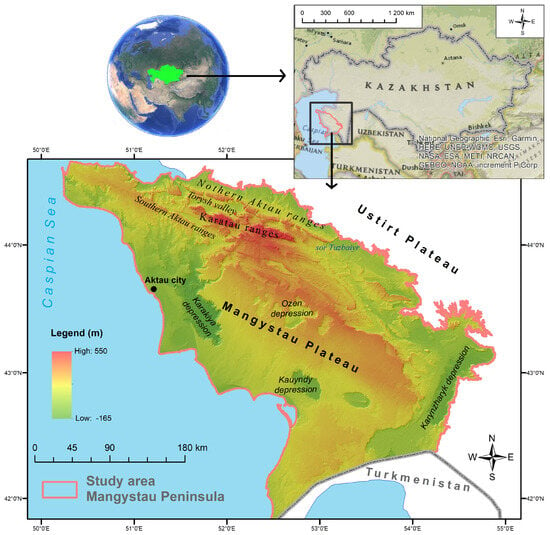
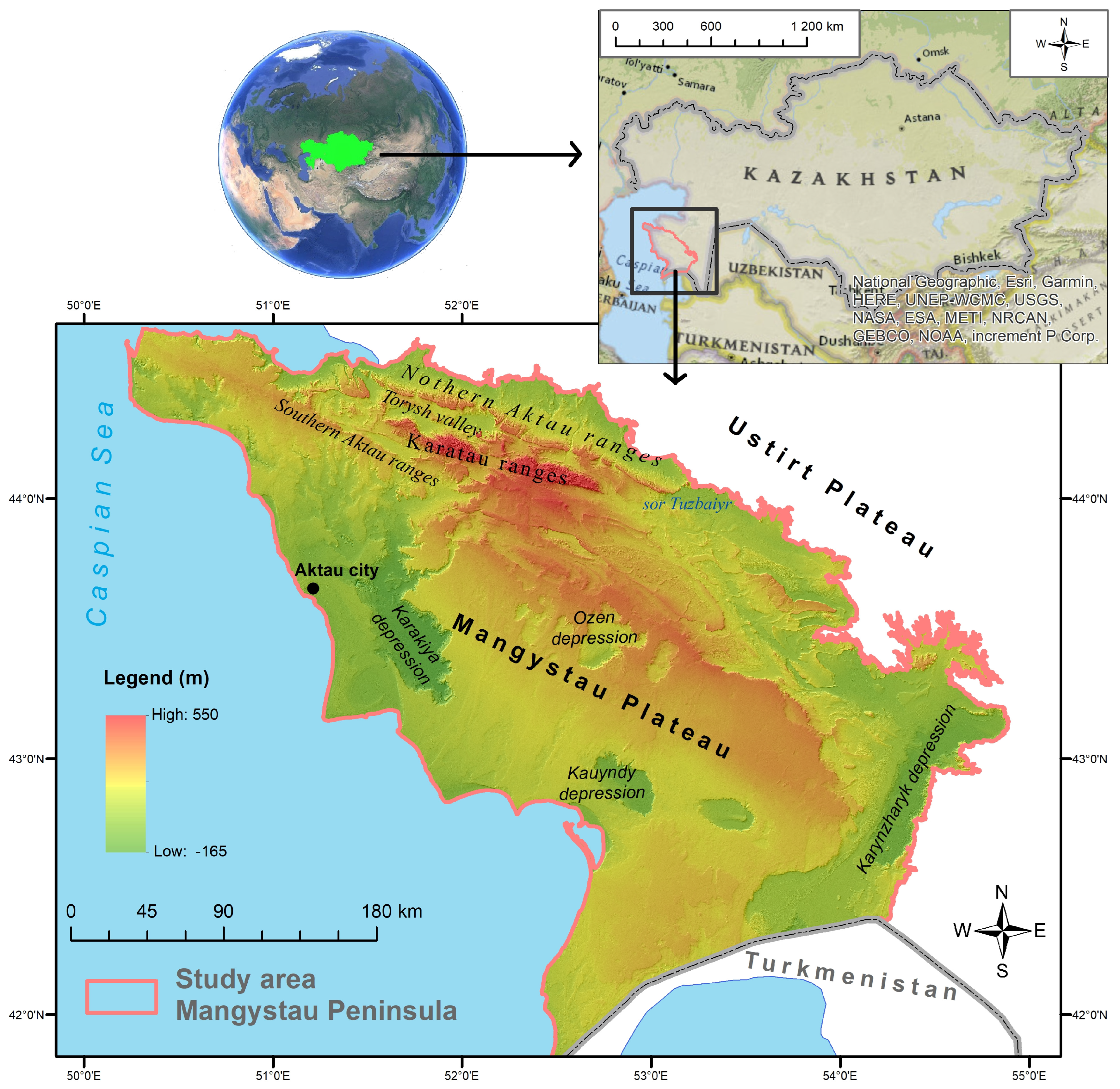
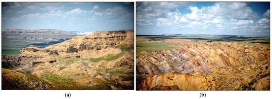
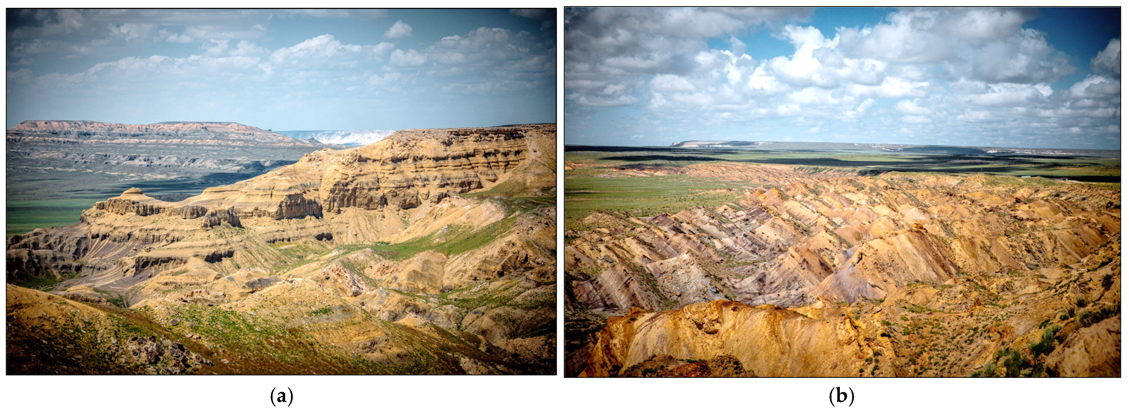
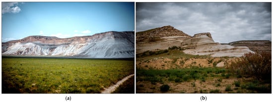
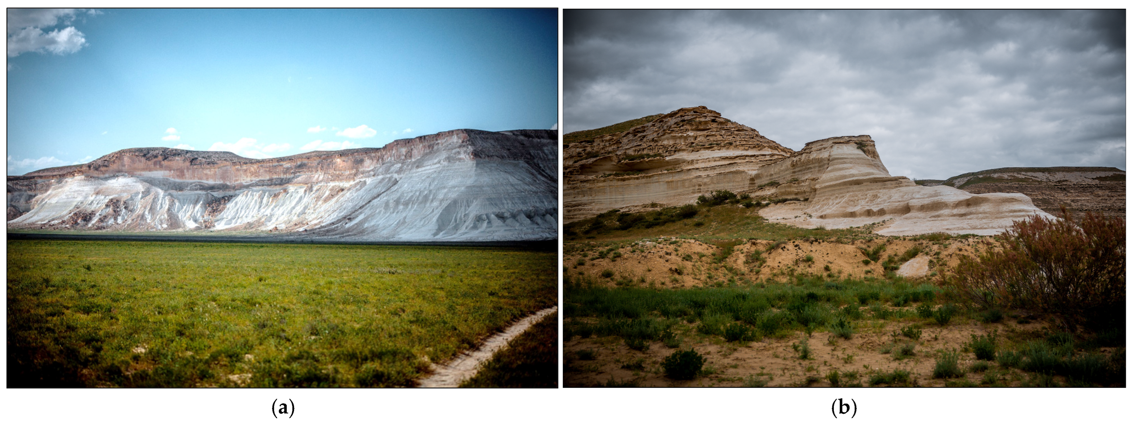
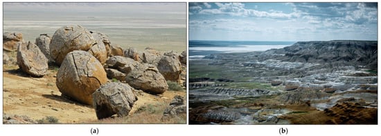
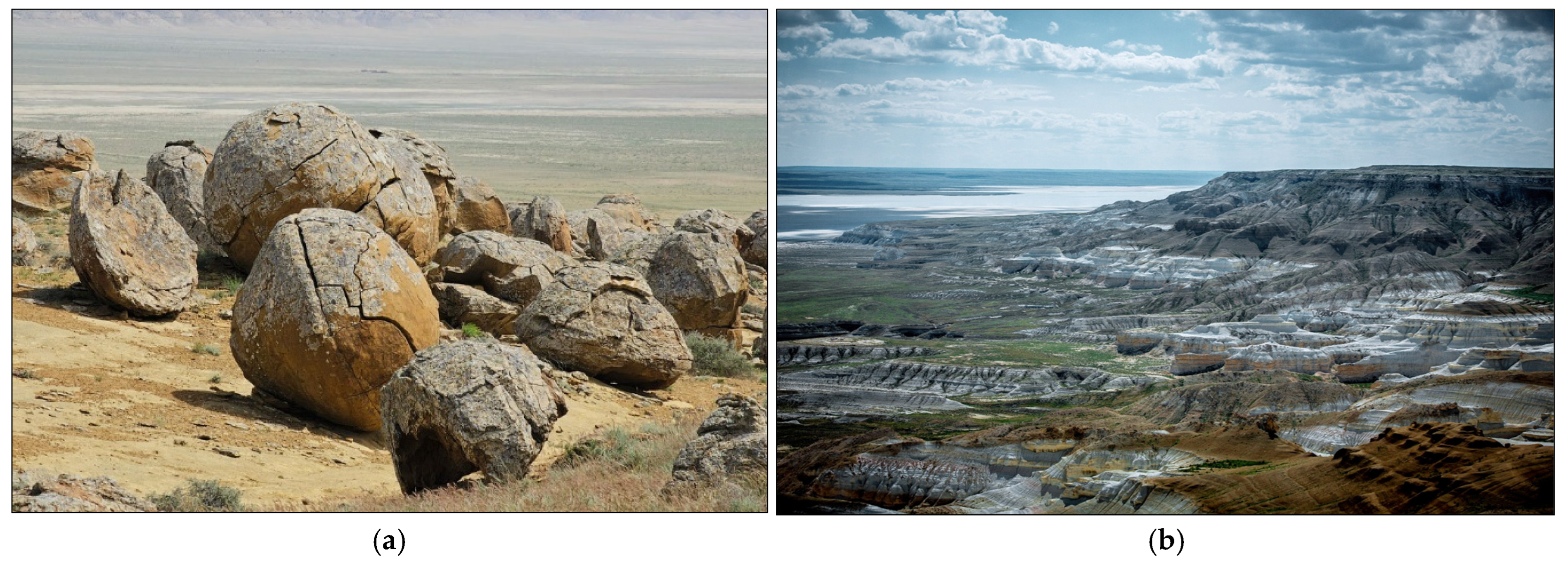
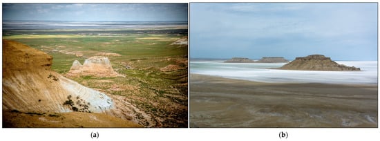
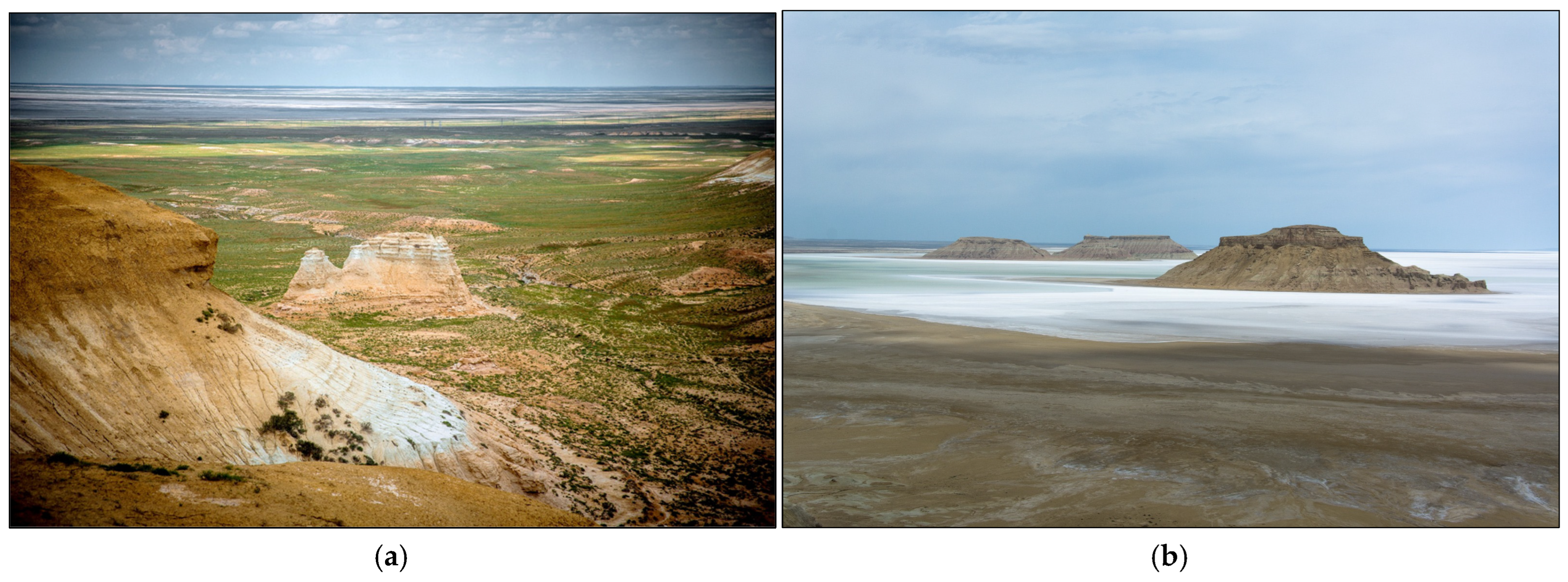
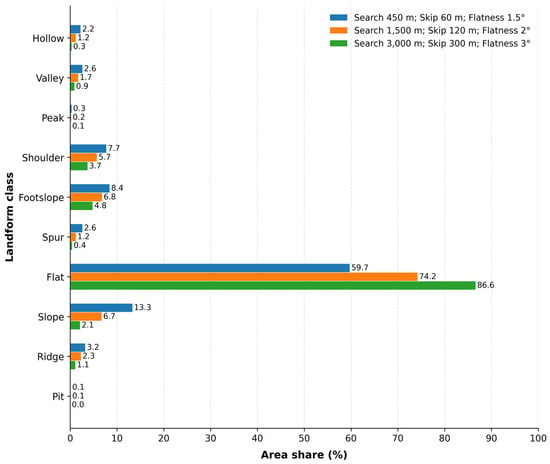
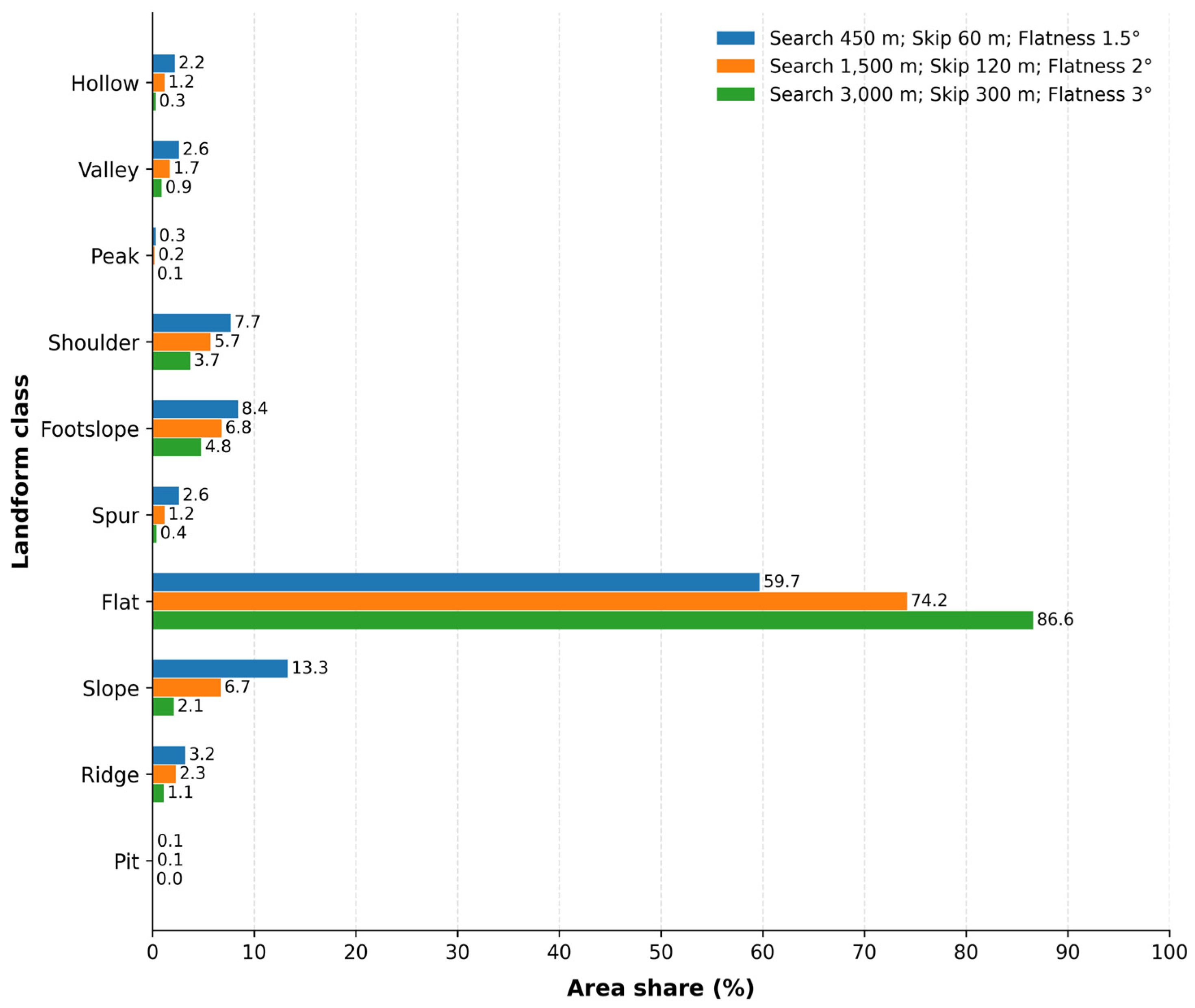
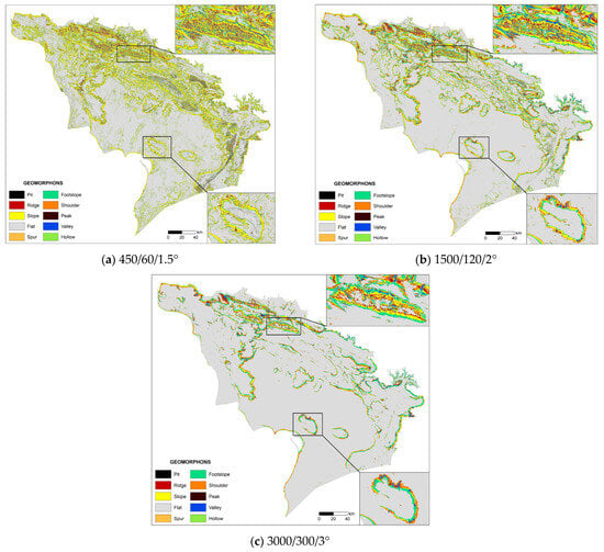
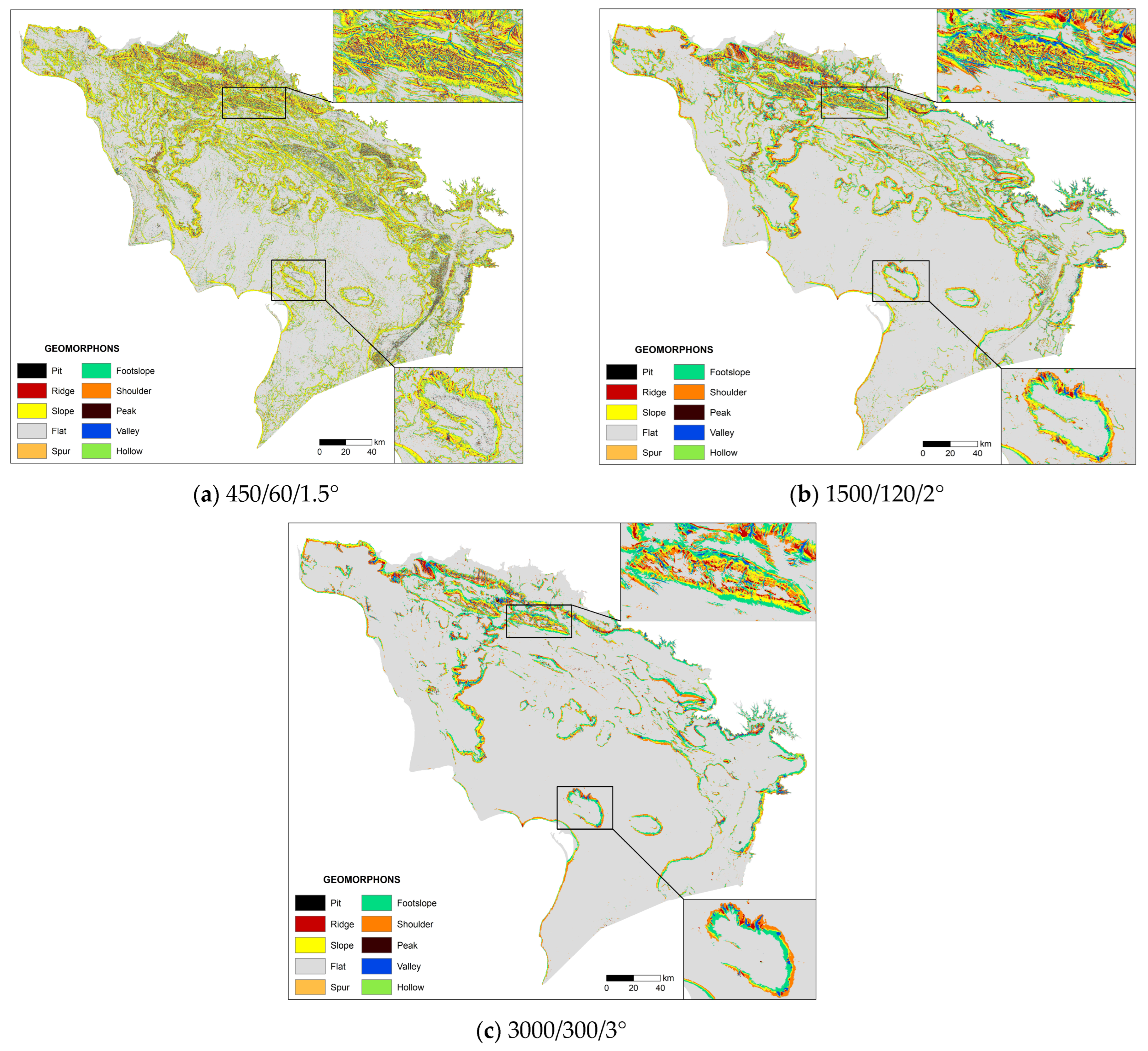
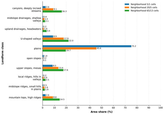
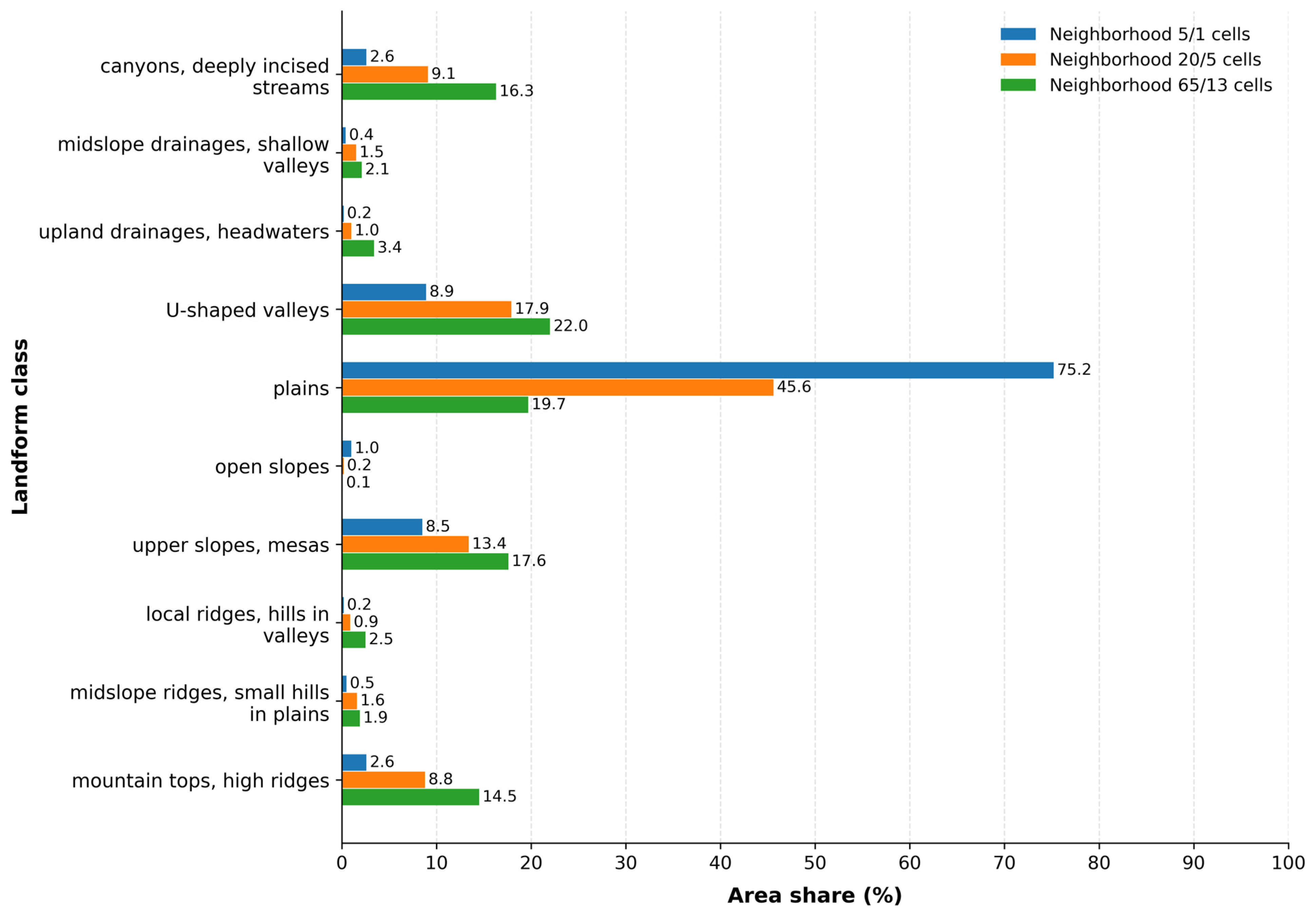
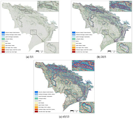
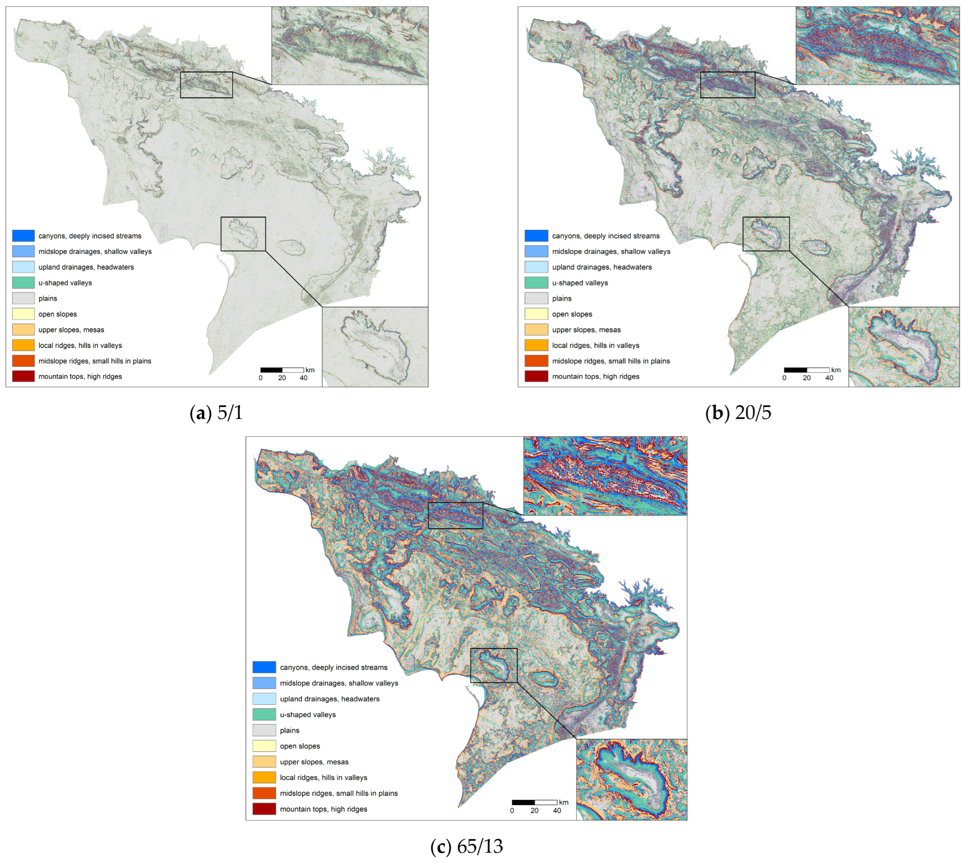
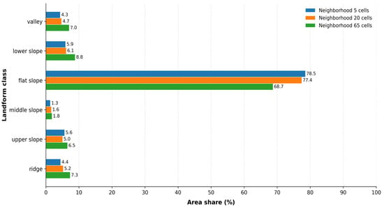
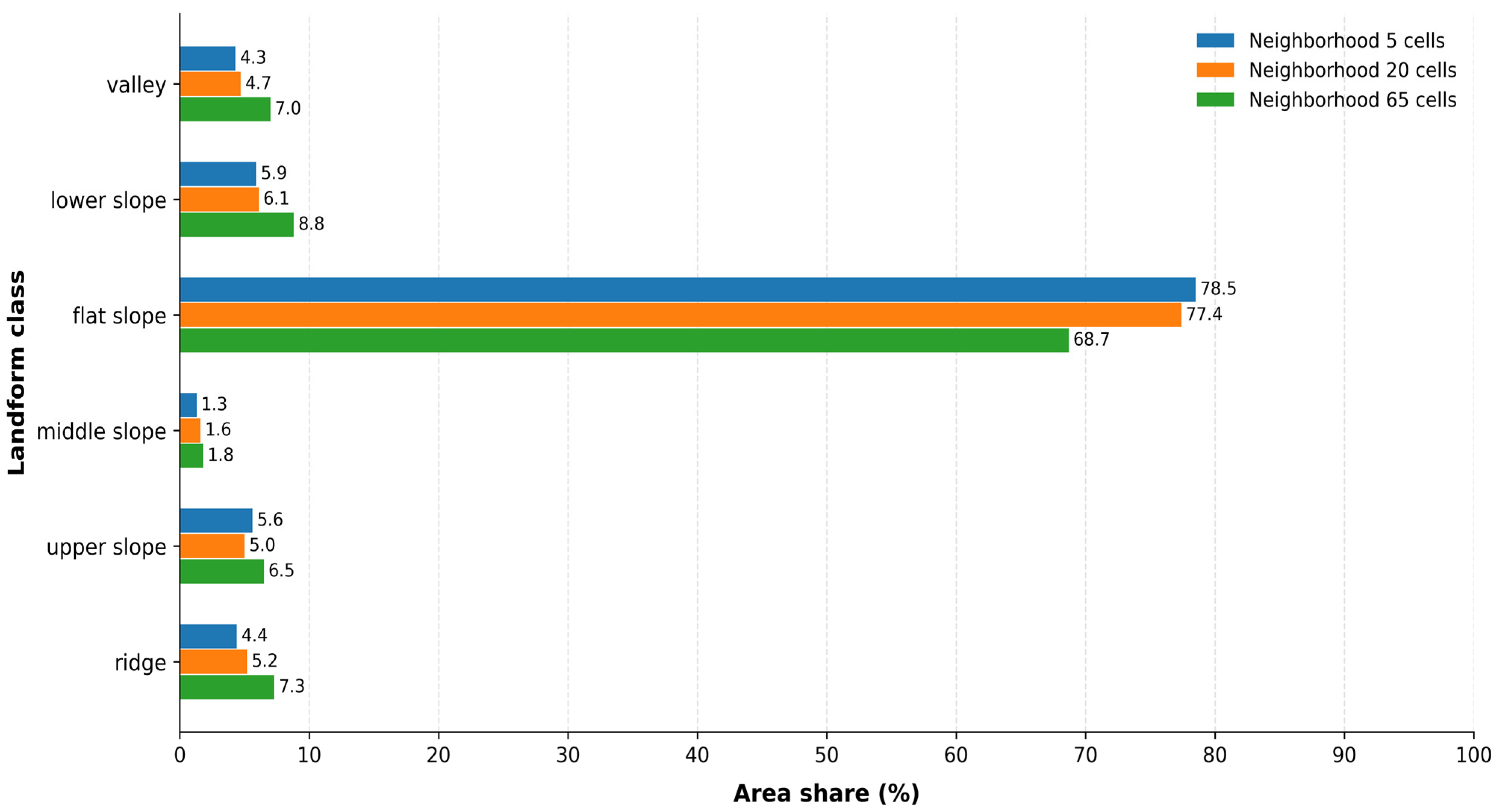
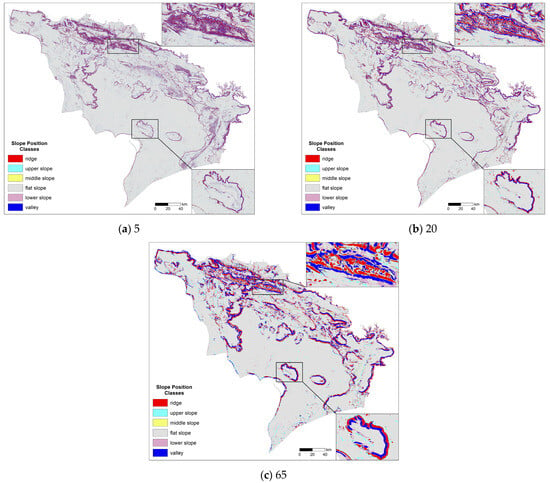
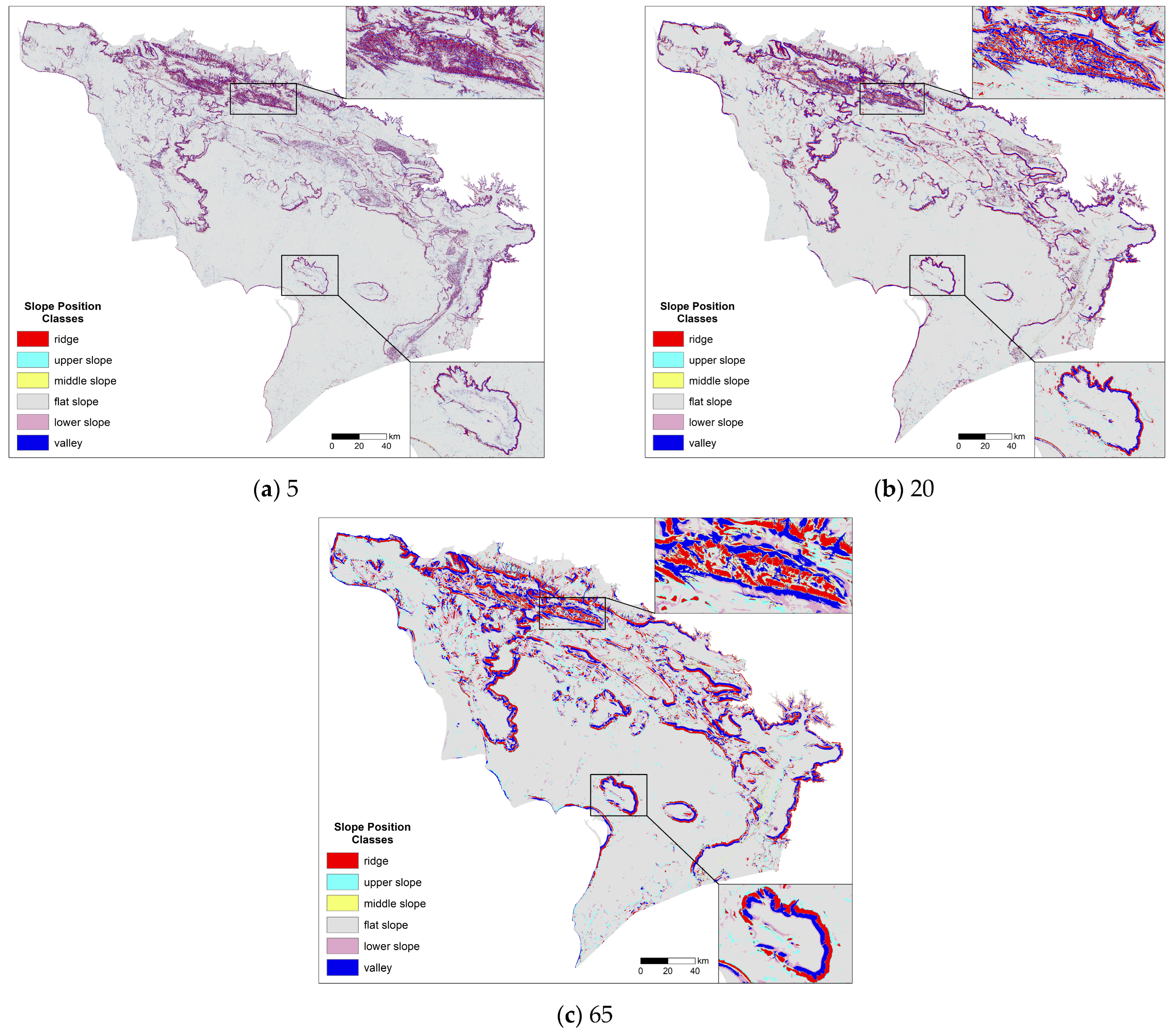

Disclaimer/Publisher’s Note: The statements, opinions and data contained in all publications are solely those of the individual author(s) and contributor(s) and not of MDPI and/or the editor(s). MDPI and/or the editor(s) disclaim responsibility for any injury to people or property resulting from any ideas, methods, instructions or products referred to in the content. |
© 2026 by the authors. Licensee MDPI, Basel, Switzerland. This article is an open access article distributed under the terms and conditions of the Creative Commons Attribution (CC BY) license.