


Abstract
Climate shocks can undermine sustainable development if lenders restrict credit precisely when households and microenterprises need liquidity. This study aims to determine whether hydroclimatic anomalies alter the placement of productive microcredit in Colombia and whether the response differs by borrower sex. We combine weekly administrative records from the Financial Superintendence of Colombia (3.98 million loans, September 2023–May 2026) with the monthly Standardized Precipitation Evapotranspiration Index (SPEI) for 1108 municipalities and estimate Poisson pseudo-maximum likelihood models with department-by-month fixed effects. An unusually wet month (SPEI ≥ 1.5) is associated with a 0.9% decline in the number of loans placed in that month, concentrated in the largest urban credit markets and among new borrowers; drought has no detectable effect, and randomization inference indicates that the evidence for the wet-month decline is modest. Credit to women does not respond differently from credit to men, although women receive loans about 18% smaller and make less use of public guarantees. The study contributes high-frequency evidence on credit flows, rather than balances, under recurrent climate anomalies. Practical implications include continuity plans for loan origination and gender-sensitive guarantee schemes. Limitations include a short panel and the inability to separate credit supply from demand.
1. Introduction
For low-income households and microenterprises, credit is one of the few formal instruments available to finance working capital, sustain consumption, and replace assets after an adverse event [1,2]. Whether this instrument remains available when a climate shock hits is not a minor issue. If lenders restrict credit placement just when liquidity needs rise, the financial system transmits and amplifies climate vulnerability; if placement is maintained, credit contributes to resilience. The question is therefore central to sustainable development: access to finance for microenterprises is part of Sustainable Development Goal (SDG) 8, gender equality in economic resources is part of SDG 5, and strengthening resilience and adaptive capacity to climate-related hazards is the core of SDG 13. The question is particularly relevant in Colombia, a country whose hydroclimatology is strongly modulated by the El Niño–Southern Oscillation. These anomalies propagate through the economy: El Niño episodes raise electricity prices in a market dominated by hydroelectric generation [3] and strengthen the link between energy prices and the stock market [4]. The 2010–2011 La Niña episode, with widespread flooding and damage to housing, infrastructure, and productive activities, showed the economic cost of excess rainfall [5,6], and global evidence indicates that daily precipitation extremes have intensified and reduce economic growth, particularly in services and manufacturing [7].
The relevance of this question extends well beyond Colombia. In South America, the extreme 1997–1998 El Niño increased problem loans at a microfinance institution in northern Peru [8], and in Mexico, extreme temperatures raise firms’ loan defaults [9]. In Asia, floods in Bangladesh tested the capacity of microfinance to act as a safety net, both through contingent repayment rescheduling [10] and through local institutions that helped households cope [11]. In sub-Saharan Africa, excess rainfall during the harvest increased the credit risk of loans to smallholders in Madagascar [12]. Cross-country evidence shows that hydrometeorological disasters raise the financial risk of microfinance institutions in about 80 developing economies [13], that microfinance lending offsets part of the growth losses caused by disasters [14], and that severe disasters raise non-performing loans most in low-income countries [15]; banking systems in less developed economies also appear less able to sustain credit supply after natural hazards [16]. In Colombia, weather shocks reduce the productivity and performance of manufacturing firms [17] and increase the share of at-risk loans in small rural municipalities, particularly for microcredit [18]. Colombia is thus a relevant middle-income case that combines high exposure to hydroclimatic variability, a large regulated microcredit market, and unusually detailed administrative data.
How credit responds to large-scale disasters is fairly well known. Banks reallocate resources toward affected areas [19], regional banks expand recovery lending after floods [20], firms draw on their credit lines after weather-related cash-flow shocks [21], and disasters weaken banks with geographically concentrated exposure [22,23]. In microfinance, credit demand increases after a disaster, but access becomes restricted for clients without a prior relationship with the lender [24], and climate shocks deteriorate portfolio quality [8,12,25]. For Colombia, credit to small potato growers increases after droughts when it is backed by public guarantees [26], the municipal microcredit portfolio grows during episodes of heavy rainfall [27], and transitory climate shocks damage coffee growers’ credit histories and restrict their future access to credit [28].
This literature leaves three issues open. The first concerns the margin of analysis and the scale of the shocks: most studies analyze outstanding loan balances, delinquency, or major disasters, rather than the monthly flow of new loans in response to frequent and moderate anomalies, which are the ones lenders face on a recurring basis. The second concerns gender. There is evidence on gaps between women and men in loan size, pricing, and collateral [29,30,31], and on differentiated climate vulnerability [32,33], but there is little evidence, based on nationwide administrative data, on whether credit placement to women and men responds differently to climate shocks. Greater vulnerability does not, by itself, imply a larger credit contraction. The third concerns identification: indices such as the SPEI are strongly spatially correlated, so their deviations from the national mean may coincide with regional credit dynamics and produce spurious associations if the empirical strategy does not account for this [34].
The objective of this paper is to determine whether recurrent hydroclimatic anomalies (unusually wet and unusually dry months) alter the monthly placement of productive microcredit in Colombia and whether this response differs between women and men, between agricultural and non-agricultural borrowers, and across rurality, new-borrower status, and access to public instruments. Colombian productive microcredit offers a suitable setting: the Financial Superintendence of Colombia (SFC) publishes weekly disbursements by lender, municipality, and loan and borrower characteristics, including the borrower’s sex; loan officers’ field assessments may be sensitive to physical disruptions and to the information available about clients [2]; and public instruments, such as rediscount funding and guarantees from the Agricultural Guarantee Fund (FAG), may mediate the response. The period analyzed, from September 2023 to May 2026, includes the drought associated with the 2023–2024 El Niño and several widespread wet episodes.
The paper makes three contributions. First, from a theoretical and empirical standpoint, it shifts attention from outstanding balances and large disasters to the flow of new microcredit under the moderate, recurrent anomalies that lenders face routinely, and it confronts competing mechanisms (agricultural income losses, operational disruptions, and information frictions in lending relationships) with nationwide administrative data. Second, it provides, to our knowledge, the first nationwide test of whether credit placement to women and men responds differently to climate anomalies, distinguishing the absence of a differential response from equality of credit conditions. Third, it offers a methodological contribution to climate-finance research by showing how spatially correlated climate indices can generate spurious effects and how within-region comparisons, placebo leads, randomization inference that respects spatial dependence, and specification curves guard against them. Together, these elements inform the design of climate-resilient and inclusive financial systems, a core concern of sustainable finance.
The remainder of the paper is organized as follows. Section 2 reviews the literature and develops the hypotheses. Section 3 describes the data and sample, the model specification, and the variables. Section 4 presents the results, organized by hypothesis. Section 5 discusses the findings, and Section 6 concludes with their theoretical and practical implications and the study’s limitations.
2. Literature Review and Hypotheses Development
2.1. Excess Rainfall, Information Frictions, and Microcredit Placement
Recent climate–economy research identifies effects from within-location variation in weather over time, which allows climate realizations to be treated as approximately random once permanent location characteristics and common period shocks are controlled for [35]. Although much of the evidence has focused on temperature, precipitation also affects growth at the subnational level [36]. Kotz et al. [7] show, using data for 1554 regions, that the number of wet days and daily rainfall extremes reduce growth and that this effect is larger in high-income countries and in the services and manufacturing sectors. Excess rainfall can therefore disrupt economic activity well beyond agriculture: Colombia’s 2010–2011 La Niña damaged housing, transport infrastructure, and non-agricultural productive sectors [5,6], and weather shocks reduce the productivity of Colombian manufacturing firms, partly through damage to road infrastructure [17].
In credit markets, such a shock moves supply and demand simultaneously and under information asymmetry. On the demand side, affected households and firms need liquidity to sustain consumption, replenish inventories, or repair assets. On the supply side, the shock raises borrowers’ perceived risk, may reduce collateral values and lenders’ funding, and hinders commercial operations. The empirical evidence reflects this ambiguity. Garmaise and Moskowitz [37] find that earthquake risk reduces the supply of credit for commercial properties in California, partly because of imperfections in the insurance market. Cortés and Strahan [19] show that financially integrated banks increase lending in disaster-affected areas and reduce it in other markets, and Koetter et al. [20] document that regional banks expand recovery lending after floods. Brown et al. [21] find that firms hit by unusually severe weather draw more on their credit lines but face tighter terms. Disasters weaken the stability of banks with exposure concentrated in affected areas [22]; in the Caribbean and Central America, tropical storms generate adverse funding shocks and an initial decline in private-sector credit [23]; and banking systems in less developed economies are less able to sustain credit supply after natural hazards [15,16]. For Colombia, municipal consumer and microcredit portfolios increase during episodes of heavy rainfall [27], a result that may reflect new disbursements as well as loan rescheduling or slower repayments.
Information asymmetries make microcredit especially sensitive to these forces. Microcredit lenders compensate for the lack of collateral and credit history with individual field assessments, soft information collected by loan officers, and repeated relationships with clients [2]. Prior relationships increase the availability of credit more than its price [38], and credit information systems reduce asymmetries between lenders and borrowers [39]. Microcredit placement therefore depends on two inputs that a wet episode can disrupt: the physical possibility of visiting and assessing clients and the information available to distinguish a transitory deterioration from a permanent one. Berg and Schrader [24] show that, after volcanic eruptions in Ecuador, credit demand increased while access was restricted except for clients with a prior relationship with the lender, and in Colombia transitory climate shocks reduce coffee growers’ credit scores and increase future loan rejections [28]. Portfolio quality also responds to excess rainfall and climate hazards [8,12,13,18,25]. Because unusually wet months disrupt mobility, commerce, and field operations, and because lenders may postpone lending when information is scarcer, we expect the supply-side and operational effects to dominate in the short run:
Hypothesis 1 (H1).
Unusually wet months (excess rainfall) reduce productive microcredit placement in the month of the shock.
2.2. Drought, Liquidity Needs, and Credit
Drought operates through a different channel. Its main effect is a gradual loss of agricultural output and income [26], with less disruption to mobility and commerce than heavy rainfall. In Colombia, dry El Niño episodes also raise electricity prices, because generation depends heavily on hydropower [3], an additional cost shock for microenterprises. Households facing income shocks with little formal insurance combine savings, informal networks, productive adjustments, and credit to smooth consumption [1], and uninsured risk, rather than lack of liquidity, constrains agricultural investment [40]. A drought can therefore raise the demand for credit to cope with the shock while making lenders more cautious about borrowers whose income has fallen. In Colombia, small potato growers’ access to credit increases after droughts, but only when loans are backed by public guarantees [26]. Because demand and supply effects push in opposite directions, the sign of the net effect is an empirical question:
Hypothesis 2 (H2).
Drought months affect productive microcredit placement, with an ambiguous sign (higher liquidity demand versus more restrictive supply).
2.3. Gender, Credit, and Climate Vulnerability
Several dimensions of the relationship between gender and credit should be distinguished. The first is access: in developing economies, gaps between women and men persist in the ownership and use of financial services [41], although in some contexts gaps in firms’ use of financial services are largely explained by firm and owner characteristics [42]. The second is loan terms. In Italy, female entrepreneurs pay higher interest rates without being riskier [29]; in small business lending, they face higher collateral requirements [30]; and in microfinance, women receive smaller loans than men, a gap that Agier and Szafarz [31] describe as a glass ceiling on loan size. The third is performance: microfinance portfolios with a higher share of women have lower risk [43], which may lead lenders to maintain their supply to this segment after a shock. The fourth is composition: experimental evidence from Sri Lanka shows that returns to capital are lower in women-owned microenterprises [44].
The fifth dimension is climate vulnerability. Climate shocks reduce welfare more in households whose land is managed by women in Malawi [32] and are associated with setbacks in women’s economic and social rights in developing countries [33]. However, greater vulnerability does not necessarily translate into a larger credit contraction. If women are less concentrated in the most exposed activities, use different products, or are perceived as better payers, their credit may respond equally or less than that of men, even when their terms are worse. For this reason, we treat the difference in the response as a hypothesis to be tested rather than as an assumption:
Hypothesis 3 (H3).
The effects of hydroclimatic shocks on microcredit placement differ between women and men.
2.4. Climate, Agricultural Activity, and Credit
Agricultural producers are directly exposed to rainfall variability, and the lack of insurance shapes their decisions [40]. In Colombian agro-industry, weather shocks affect sugar prices together with the pass-through of international prices [45]. In Colombia, rainfall variability reduces disbursements backed by private guarantees to small potato growers, whereas public guarantees allow credit to expand after droughts [26]. Agricultural exposure therefore has two potential effects on the credit response: it may amplify the contraction, through the deterioration of borrowers’ income and risk, or attenuate it if the shock generates demand for credit to cope with it and public instruments allow lenders to meet that demand. Because the literature on climate and agricultural credit emphasizes the first channel [8,12,13], we state the hypothesis in that direction:
Hypothesis 4 (H4).
The effects of hydroclimatic shocks on microcredit placement are larger for agricultural borrowers.
2.5. Rurality, Lending Relationships, and Public Instruments
Three further dimensions may condition the response. The first is rurality. If excess rainfall operates mainly through agricultural losses, the response should be concentrated in rural municipalities; if it operates through disruptions to commerce, transport, and services, it may be concentrated in urban centers, where retail and service microenterprises cluster [7]. Official classifications of rurality, rather than lending-based proxies, are needed to test this distinction [46,47]. The second is the lending relationship. New borrowers, about whom the lender has less information, should be more sensitive to shocks than repeat borrowers [24,28,38]. The third is access to public instruments. Recapitalized microfinance lending supported recovery after the 2004 tsunami in Sri Lanka [48], microfinance offsets part of disasters’ growth costs [14], and public guarantees allow credit to work as a coping mechanism among small producers [26]. Rediscount funding, FAG guarantees, and public development banking may therefore buffer the credit response:
Hypothesis 5 (H5).
The effects of hydroclimatic shocks on microcredit placement vary with rurality, new-borrower status, and access to public instruments (rediscount funding, FAG guarantees, and public development banking).
3. Materials and Methods
3.1. Data and Sample
Credit data come from the SFC public dataset on lending interest rates by loan type, which reports weekly the weighted average effective rate, the amount, and the number of loans disbursed by lender, municipality, and loan and borrower characteristics [49]. We use the records of productive microcredit granted to individual borrowers, both women and men, and to micro and small enterprises. The analysis period, from September 2023 to May 2026 (33 months), coincides with the period in which the regulatory classification of productive credit and productive popular credit has been in force. Weekly reports are assigned to the calendar month of their weekly reporting date; as a result, months that contain five weekly cut-offs record about 28% more loans than months with four (the correlation between monthly loans and the number of Fridays in the month is 0.84). This mechanical calendar pattern is common to all municipalities and is absorbed by the month fixed effects described below. September 2023 contains only the first weeks under the new classification, which is why we also report estimates that exclude it.
Because the source reports only combinations of characteristics with positive disbursements, a missing combination is a genuine zero provided that the lender was reporting in that week. Supervised lenders are required to report weekly, and 15 of the 22 lenders report in all 33 months and account for 91.6% of the loans; the remaining lenders enter or exit during the period (for example, one bank begins reporting in March 2024 and another stops in August 2024). Lender entry and exit are absorbed by the lender-by-month fixed effects of the within-lender design, and the main estimates are similar when the panel is built only with lenders that report in every month (Section 4.4).
Table 1 traces the sample from the original records to the estimation sample. The source contains 3,357,402 lender–municipality–characteristics–month records, without duplicates, from 22 supervised lenders, which group 4,186,275 loans; each record groups one or more loans, so the number of records does not match the number of loans. We exclude 179,186 records (202,885 loans) without information on the disbursed amount and rate, 98% of which come from a single lender. The remaining 3,178,216 records, with 3,983,390 loans, are aggregated into municipality–sex–month cells and completed with zeros. All 1108 municipalities with productive microcredit are matched to the climate data. The Poisson estimator drops 299 cells that belong to fixed-effect groups with only zeros, yielding an estimation sample of 72,829 cells.
Table 1.
Sample construction: from source records to the estimation sample.
Climate data correspond to the monthly municipal SPEI at a one-month scale (SPEI-1), a standardized index of the climatic water balance (precipitation minus potential evapotranspiration) relative to each municipality’s climatology for each calendar month [50]. Negative values indicate drier-than-normal conditions and positive values indicate wetter-than-normal conditions. The municipal climate panel covers January 1981 to May 2026 for 1119 municipalities and was built from daily gridded data: precipitation from the Climate Hazards Group InfraRed Precipitation with Station data (CHIRPS, version 2.0, Climate Hazards Center, University of California, Santa Barbara; 0.05° resolution, about 5.5 km) [51] and daily maximum and minimum near-surface air temperature from ERA5-Land (Copernicus Climate Change Service, European Centre for Medium-Range Weather Forecasts; 0.1° resolution, about 9 km) [52], downloaded in 09-2026. Daily grids were assigned to municipalities as the area-weighted mean of the grid cells that intersect each municipal polygon of DANE’s National Geostatistical Framework [53] and aggregated to calendar months (sums for precipitation and means for temperature). Potential evapotranspiration was estimated with the Thornthwaite method [54] from monthly mean temperature (the average of daily maximum and minimum) and latitude, and the SPEI-1 was computed with the R package SPEI (version 1.8.1) [55], which fits a log-logistic distribution by unbiased probability-weighted moments for each municipality and calendar month, using the full record (January 1981–May 2026) as the calibration period.
Three features of the data describe the spatial matching and the identifying variation. First, because climate values are area-weighted means over each municipal polygon, no two municipalities share an identical climate series; in the estimation period, 172 of the 1108 municipalities have an SPEI series correlated above 0.99 with that of another municipality, mostly small neighboring municipalities. Second, department-by-month fixed effects absorb 73% of the variance of the SPEI, but substantial variation remains: the within-municipality, within-department-month standard deviation of the SPEI is 0.55 (against 1.12 in the raw data), and 93% of the municipality-months with SPEI ≥ 1.5 occur in department-months in which other municipalities do not reach that threshold. Third, positive SPEI anomalies closely track precipitation: the correlation between the SPEI-1 and a standardized precipitation index computed from CHIRPS alone (SPI-1) is 0.96, 93.5% of the months with SPEI ≥ 1.5 also have SPI ≥ 1.5, and 99.6% have precipitation at or above the local 90th percentile. Appendix A Table A3 reports these diagnostics.
We use an official classification of rurality, the municipal rurality categories defined by the National Planning Department (DNP) and the Mission for the Transformation of the Countryside, which classify municipalities as cities and agglomerations, intermediate, rural, or dispersed rural on the basis of membership in the System of Cities, population density, and the share of the population outside the municipal seat [46]. This classification replaces the indicator used in the previous version of the paper, which was derived from the rural label of the credit products observed in each municipality and could therefore reflect lending composition rather than the municipality’s underlying characteristics (Appendix A Table A6 compares both classifications). Because the DNP categories were fixed with 2014 data, they are predetermined with respect to the study period. Of the 1108 municipalities in the sample, 117 are cities and agglomerations, 312 are intermediate, 373 are rural, and 306 are dispersed rural; the last two groups, which the DNP treats as rural, account for 27.8% of the loans. Municipal boundaries come from DANE’s National Geostatistical Framework [53].
3.2. Model Specification
Because the source reports only positive disbursements, we aggregate loans into municipality–sex (and, where relevant, loan characteristic)–month cells and complete the Cartesian product with zeros, which avoids conditioning the analysis on positive placement. The outcomes are counts with zeros and a highly skewed distribution. We therefore use Poisson pseudo-maximum likelihood (PPML) with high-dimensional fixed effects, an estimator that is consistent under heteroskedasticity and avoids the retransformation bias of log-linear models [56]:
where Y is the number (or amount) of loans in municipality m, for sex s, in month t; Rain and Drought are the excess-rainfall and drought indicators, respectively, with non-extreme months as the reference; αms are municipality-by-sex fixed effects, which absorb permanent differences in market size, banking structure, and client composition; and δs,d(m),t are sex-by-department-by-month fixed effects. The expression 100·(exp(β) − 1) measures the percentage change in placement in a shock month relative to a normal month in the same municipality.
E[Ymst | ·] = exp(βWRainmt + βDDroughtmt + αms + δs,d(m),t)
Identification. The empirical strategy relies on the idea that, conditional on location and period fixed effects, the local climate anomaly behaves as a random realization [35]. A municipality’s monthly water-balance anomaly, standardized relative to its own climatology, cannot be caused by credit placement, which rules out reverse causality. The relevant threat is confounding. The SPEI is strongly spatially correlated, so its deviations from the national mean may coincide with regional economic and credit dynamics [34]. Department-by-month fixed effects compare municipalities in the same department in the same month, so identification comes from local differences in anomalies. The identifying assumption is that, conditional on these fixed effects, local anomalies are independent of non-climate credit shocks. We test this assumption with shock leads in an event study, since future weather should not affect current credit [57]; with placebo tests that reassign climate series (described below); and with a within-lender design that absorbs the funding, strategy, and supply shocks common to each lender [58].
Fixed versus random effects. The choice of unit fixed effects rather than random effects was tested formally. A Hausman test [59] comparing within- and random-effects estimators of the linear model for the inverse hyperbolic sine of loans, after partialling out the sex-by-department-by-month effects, rejects the consistency of the random-effects estimator (χ2(2) = 125.4; p < 0.001). Because the classical test assumes efficiency of the random-effects estimator under the null, we also report the cluster-robust Mundlak (correlated random effects) version [60], which adds the cell means of the shock indicators to a pooled model: their joint significance is rejected in the linear model (p = 0.028) and marginally in the Poisson model (p = 0.085) (Appendix A Table A7). Exposure to wet and dry months is therefore correlated with unobserved municipal characteristics, and the fixed-effects estimator, which is consistent in either case, is the appropriate choice.
Dynamics. Rainfall shocks are recurrent and non-absorbing, so staggered difference-in-differences estimators built around the first treatment do not apply [61]. We estimate distributed-lag models with two leads and three lags, which are equivalent to event studies with multiple events [57]:
where k indexes leads (k < 0) and lags (k > 0) of the excess-rainfall and drought indicators. We report the full set of coefficients, joint tests of the leads and of the lags, and cumulative effects up to each horizon with their confidence intervals. We also estimate local projections for horizons of 0 to 6 months [62]:
where the controls include two lags of both shocks. Because wet months are mildly persistent (the probability of a wet month is 0.22 after a wet month and 0.09 unconditionally), the local projection at horizon h combines the effect of the initial shock with that of any subsequent shocks correlated with it; we therefore also report projections that control for the shocks between t + 1 and t + h, and we distinguish the first month of a wet episode from its continuation.
E[Yms,t+h | ·] = exp(βhRainmt + θhDroughtmt + X′mtφh + αms + δs,d(m),t), h = 0, …, 6
Heterogeneity and within-lender models. The heterogeneity analysis interacts the shocks with a group indicator G (for example, women, agricultural borrowers, or rural municipalities). For characteristics of the loan or borrower, the panel is disaggregated into municipality–sex–group–month cells (c), and the model includes cell fixed effects and sex-by-group-by-department-by-month fixed effects:
E[Yct | ·] = exp(βRainmt + γRainmt × Gc + θDroughtmt + κDroughtmt × Gc + αc + δs,G,d(m),t)
For municipal characteristics (rurality), the same specification is estimated on the municipality–sex panel, with the group-specific department-by-month effects; for sex, the model uses the municipality–sex panel with the baseline fixed effects. We report the interaction coefficients γ and the group-specific total effects, β + γ, with their confidence intervals. The within-lender design is estimated on lender–municipality–sex–month cells (ℓ indexes lenders):
where αℓms are lender–municipality–sex fixed effects and λℓ,s,t are lender-by-sex-by-month fixed effects, which absorb lender-wide supply shocks; the second version adds sex-by-department-by-month fixed effects. The panel has 9497 lender–municipality pairs and 626,802 potential cells; the effective samples (550,626 and 550,622 cells) are smaller because PPML drops fixed-effect groups with only zeros. Estimation samples differ from the 73,128 cells of the balanced panel for the same reason and because disaggregated panels have more cells.
E[Y𝓁mst | ·] = exp(βRainmt + θDroughtmt + α𝓁ms + λ𝓁,s,t)
Inference. Standard errors are clustered by municipality, the level at which treatment is assigned [63]. Given the spatial correlation of the SPEI [64], we also report standard errors clustered by department (32 clusters) and two-way clustered by municipality and department-month; Conley standard errors [65] with 100 and 250 km cutoffs, computed with a uniform kernel on great-circle distances between municipal centroids and without a temporal cutoff, so that all observations within the distance band are allowed to be correlated at any lag; and Driscoll–Kraay standard errors, which are robust to cross-sectional and serial correlation of general form [66]. We also report estimates that exclude one department at a time. All models were estimated in R (version 4.3.3; R Foundation for Statistical Computing, Vienna, Austria) with the fixest package (version 0.14.2).
Randomization inference. We use two placebo procedures. The first reassigns complete climate series across municipalities within the same department (1000 permutations). It preserves the temporal structure of each series and the department-level distribution of shocks, but it breaks the spatial dependence between neighboring municipalities, so its validity rests on exchangeability of series within departments. The second, which preserves spatial dependence exactly, assigns to all municipalities simultaneously the SPEI observed in the same calendar months of an earlier window (September of year Y to May of year Y + 3, for Y = 1981, …, 2020; 40 placebo windows). Both p-values are two-sided and computed as (1 + Σr 1[|βr| ≥ ||])/(1 + R), where R is the number of placebo draws; we also report one-sided p-values.
Pre-specification and multiple testing. The outcomes, shock definitions, fixed effects, hypotheses, and robustness specifications of the main analysis were fixed in a dated analysis plan (25 September 2026) written before estimation, which is included in the replication package (see the Data Availability Statement). The pre-specified analyses are the specification curve, which includes the baseline model, the local projections, the within-lender design, the Conley standard errors and leave-one-department-out estimates, the agricultural-exposure interaction, the extensive margin, and the heterogeneity tests. The event study, the within-department permutation placebo, the binned SPEI specification, and the secondary outcomes are complementary diagnostics. The analyses added in response to the review (the official rurality classification, the validation with precipitation-only indices, the moderate-shock sensitivity, alternative exposure windows, the estimator comparison on a common sample, the market-size heterogeneity, the aggregated counterfactual, the historical placebo, Driscoll–Kraay standard errors, and the Hausman tests) are exploratory and are labeled as such. The specification curve [67] varies the outcome (number of loans and amount), the shock measure (±1.5 thresholds, ±2 thresholds, and continuous index), the estimator (PPML, ordinary least squares (OLS) on the inverse hyperbolic sine, and negative binomial), the time fixed effects, and the sample, and comprises 126 models for the average effect and 126 for the interaction with sex. Heterogeneity tests are corrected for multiple testing using the Holm procedure [68].
3.3. Variables
Table 2 summarizes the definition, source, and rationale of each variable. The variables are grouped as dependent variables, independent (shock) variables, moderators used in the heterogeneity analysis, and controls.
Table 2.
Variables: definition, source, and rationale.
Dependent variables. The main outcome is the number of loans disbursed in each cell, the variable closest to the credit-placement margin: a disruption to client flows or loan officers’ field work, or a more cautious lending decision, appears first as fewer loans. The disbursed amount is the co-primary outcome because it captures the volume of liquidity provided and may adjust through loan size as well as through the number of loans. The secondary outcomes (the average loan amount, the interest rate on fixed-rate loans, and the share of new borrowers) help distinguish price rationing, which would raise rates, from quantity rationing and selection of clients. Because the data report loans rather than borrowers, and borrowers may obtain more than one loan, changes in the number of loans should not be read as changes in the number of people with access to credit.
Independent variables. Excess rainfall (unusually wet month) is an indicator equal to one when SPEI-1 ≥ 1.5 and drought is an indicator equal to one when SPEI-1 ≤ −1.5; both thresholds correspond to severe anomalies in the standard SPEI classification and to roughly the top and bottom 7% of a standard normal distribution, which isolates months that depart clearly from local climatology. Because the SPEI measures the climatic water balance rather than precipitation alone, we validate the excess-rainfall indicator against precipitation-only measures (SPI-1 ≥ 1.5 and precipitation above the local 90th percentile) and, following the reviewers’ suggestion, describe the exposure as unusually wet conditions; interpretations involving floods or transport interruptions are offered as possible channels, not as measured exposures. The extreme thresholds (±2), the continuous index, and a split between moderate (1.5 ≤ SPEI < 2) and extreme (SPEI ≥ 2) wet months are used as alternatives.
Moderators. The heterogeneity variables correspond to the mechanisms in Section 2. Sex (H3) identifies borrowers recorded as women. The agricultural indicator (H4) identifies borrowers whose activity belongs to Section A of ISIC Rev. 4; it refers to the borrower’s activity, not to the purpose of the loan. We also use the agricultural share of each municipality’s loans in an initial window as a continuous exposure measure, estimated only for the months after that window so that it is predetermined (Section 4.5). Rurality (H5) is the official DNP classification described above. A new borrower (H5) is a client without a previous credit with the reporting lender, as recorded by the lender in the SFC report (category “Nuevo”, as opposed to “Recurrente”); this definition refers to the relationship with the reporting lender and does not imply that the borrower is a first-time formal borrower. Rediscount funding, FAG guarantees, and public development banking (H5) identify loans funded with rediscount resources, guaranteed by the FAG, or granted by the public agricultural development bank. Productive popular credit identifies the regulatory segment of smaller productive loans.
Controls. The model does not include time-varying municipal covariates. Local economic activity, employment, or prices are plausible outcomes of the climate shock, and conditioning on them would introduce bad-control bias [35]. Instead, the municipality-by-sex fixed effects absorb permanent differences across markets, the sex-by-department-by-month fixed effects absorb national and regional shocks, seasonality, the calendar composition of weekly reports, and regional credit cycles, and the wet and dry indicators are included jointly so that each is estimated relative to non-extreme months. The dynamic models add leads and lags of both shocks, and the local projections control for previous shocks. Municipality-by-calendar-month fixed effects, which absorb municipality-specific seasonality, are used as a robustness check.
4. Results
4.1. Data Overview
Table 3 summarizes the data. Productive microcredit is highly fragmented: the median record contains one loan, and the average loan is around 10 million pesos. Panel A describes all 3,357,402 records, including the 179,186 records without amounts; the panel in Panel B is built from the 3,178,216 records with amounts, which contain 3,983,390 loans. This difference explains why multiplying the number of records by the mean number of loans per record in Panel A (4.19 million loans) exceeds the loan totals reported in Table 4 (3.98 million), which coincide with the panel. The interest rates in Table 3 and Table 4 and in the secondary-outcome analysis (Section 4.6) also refer to different weightings: Table 3 reports the simple mean across fixed-rate records (55.1%), Table 4 the mean weighted by the number of loans (55.8%), and the secondary-outcome analysis the amount-weighted rate within each cell averaged across cells with the number of loans as weights (45.9%). Because larger loans carry lower rates, amount weighting yields lower averages (the amount-weighted mean across records is 45.1%).
Table 3.
Descriptive statistics.
Table 4.
Loan characteristics by borrower sex.
The SPEI-1 has a mean of −0.11 and a standard deviation of 1.12 in the study period, so the period was slightly drier than the 1981–2026 climatology, in line with the 2023–2024 El Niño. Its distribution has a strong national component (Figure 1). Drought dominated the beginning of the period: 63% of municipalities were in drought in September 2023 and 81% in January 2024. Widespread wet episodes occurred in June 2024 (29% of municipalities with SPEI ≥ 1.5), February 2025 (39%), and January and February 2026 (71% and 45%). Department-by-month fixed effects absorb 73% of the variance of the index, which shows why comparisons that only rely on national time effects are vulnerable to regional confounding, and why the preferred specification compares municipalities within the same department and month.
Figure 1.
Monthly municipal SPEI-1 and share of municipalities in shock, September 2023 to May 2026. The black line shows the mean SPEI-1 across municipalities and the grey area its interquartile range (left axis). Blue bars above zero show the share of municipalities with excess rainfall (SPEI-1 ≥ 1.5), and orange bars below zero show the share with drought (SPEI-1 ≤ −1.5) (right axis). Dashed horizontal lines mark SPEI-1 = 1.5 and SPEI-1 = −1.5.
Exposure to hydroclimatic shocks is frequent but not universal. Months with excess rainfall account for 9.0% of municipality-months, months with extreme excess rainfall (SPEI ≥ 2) for 2.4%, and drought months for 12.0%. Across municipalities, the median share of wet months is 9.1% (interquartile range 6.1–12.1%), 4.4% of municipalities never experienced a wet month in the period, and the maximum share is 39%; for drought, the median is 12.1% and the maximum 52%. Exposure is similar across rurality categories (9.7% of months with excess rainfall in cities and agglomerations and 8.9% in intermediate, rural, and dispersed rural municipalities), so differences in the credit response across these categories are unlikely to reflect differences in exposure. Wet months are mildly persistent: the probability of a wet month is 0.22 after a wet month and 0.09 otherwise. Figure 2 shows the geographic distribution of exposure and the official rurality categories.
Figure 2.
Exposure to hydroclimatic shocks and official rurality categories: share of months with (a) SPEI ≥ 1.5 and (b) SPEI ≤ −1.5 by municipality, and (c) DNP rurality category (2014). Boundaries: DANE National Geostatistical Framework.
Women receive 54.0% of loans but only 47.7% of the amount, because their loans are smaller (8.6 versus 11.1 million pesos). Conditional on the month, the average amount of their loans is about 18% lower, while the difference in the interest rate on fixed-rate loans is small and not significant (0.21 percentage points; p = 0.19) (Table 4). The size gap has an economic interpretation in terms of portfolio composition. Women are much less likely to be agricultural borrowers (20.4% versus 35.4%) and to borrow in rural municipalities (24.7% versus 31.5% of loans, using the DNP classification) and more likely to use productive popular credit (69.1% versus 60.8%), a regulatory segment of smaller loans. They also obtain fewer loans with maturities above three years (13.2% versus 18.6%) and make much less use of FAG guarantees (11.6% versus 20.6%) and rediscount funding (12.2% versus 22.1%), instruments concentrated in agricultural lending. The gender gap therefore operates mainly through loan size, product mix, and access to public instruments rather than through prices, although the rate comparison does not control for borrowers’ risk profiles.
Figure 3 shows credit placement over time by sex. The saw-tooth pattern of both series is a calendar effect of weekly reporting: months with five weekly cut-offs record about 28% more loans than months with four, which is why all specifications include month fixed effects. Beyond this pattern, placement to women and men moves in parallel; women obtain more loans than men in every month, but men receive larger amounts, so the gap documented in Table 4 is stable over the period rather than the result of particular episodes.
Figure 3.
Monthly productive microcredit placement by borrower sex.
4.2. Baseline Estimates: Excess Rainfall (H1) and Drought (H2)
Table 5 presents the baseline estimates. With national time fixed effects (column 1), excess rainfall is associated with fewer loans and drought with more, and the continuous index has a negative and significant coefficient. When department-by-month fixed effects absorb regional shocks (column 2, preferred specification), the excess-rainfall coefficient is −0.0087 (SE 0.0042; p = 0.036), equivalent to a 0.87% reduction in the number of loans (95% confidence interval: −1.67% to −0.06%), while the drought coefficient falls practically to zero and the continuous-index coefficient is no longer significant. When municipality-by-calendar-month fixed effects are added to absorb local seasonality (column 3), the excess-rainfall estimate remains negative and significant and is somewhat larger in magnitude (−0.0131). The negative binomial and OLS inverse-hyperbolic-sine estimates (columns 4 and 5), which weight municipalities more evenly, show no reduction: the former is close to zero and the latter is positive and only marginally significant (p < 0.1). The response of the disbursed amount (column 6) is −0.75% (95% CI: −1.77% to +0.28%). Its point estimate is close to that for the number of loans, and a stacked PPML model that estimates both responses jointly does not reject their equality (difference of −0.12 percentage points; p = 0.79). The evidence therefore supports a small decline in the number of loans and a similarly negative but less precisely estimated response of amounts, not a differential effect on counts and amounts.
Table 5.
Rainfall shocks and microcredit placement: baseline estimates.
The excess-rainfall result is not specific to the evapotranspiration component of the SPEI. Using an index based only on CHIRPS precipitation, an unusually wet month (SPI-1 ≥ 1.5) reduces the number of loans by 0.68% (p = 0.045). The effect is driven by moderate anomalies: months with 1.5 ≤ SPEI < 2 reduce loans by 0.86% (p = 0.043), the coefficient for extreme months (SPEI ≥ 2) is similar but imprecise (−0.89%; p = 0.28), and excluding municipality-months with |SPEI| ≥ 2 leaves the estimate unchanged (−0.85%; p = 0.047). In contrast, a broader indicator of precipitation above the local 90th percentile, which flags 14.7% of municipality-months (39% of them with SPEI below 1.5), has no effect, which suggests that the response is limited to clearly anomalous months. Because the SPEI and SPI indicators overlap in 93.5% of wet months, neither is significant when both are included, so the data cannot separate precipitation from evaporative demand (Appendix A Figure A3).
Assessment of H1. The evidence is consistent with H1 in the direction predicted, but the effect is small and confined to the number of loans in the month of the shock; Section 4.3 and Section 4.4 show that its statistical strength is modest once inference accounts for spatially correlated shocks and that it depends on the largest credit markets. Assessment of H2. H2 is not supported: once regional shocks are absorbed, drought has no detectable effect on the number of loans (0.10%; p = 0.81) or on the amount (0.46%; p = 0.38), and the positive association obtained with national time effects fails the placebo tests described next.
4.3. Identification Tests
Table 6 and Figure 4 present the event study, estimated on the common sample from December 2023 to March 2026 allowed by the leads and lags. With national time fixed effects, the drought leads are large and jointly significant (p = 0.001): a drought that will occur two months later is associated with more loans today. This placebo failure indicates that the positive drought coefficient in column 1 of Table 5 cannot be interpreted as a causal effect and probably reflects regional credit dynamics that coincided with the 2023–2024 dry period. With department-by-month fixed effects, all leads are small and not jointly significant (p = 0.54 for excess rainfall and 0.41 for drought), a result consistent with the identifying assumption. In this specification, the lags of excess rainfall are not jointly significant (p = 0.13). The cumulative coefficient is −0.0076 in the month of the shock (95% CI: −0.0158 to 0.0005), −0.0135 after one month (−0.0281 to 0.0010), and −0.0077 after three months (−0.0314 to 0.0159). The confidence intervals of the cumulative effects are wide: they rule out cumulative declines larger than about 3.1% after three months, but they do not allow us to conclude that the effect disappears. Appendix A Table A2 reports all the coefficients of the dynamic specifications.
Table 6.
Event-study diagnostics: cumulative effects, joint tests, and randomization inference.
Figure 4.
Event-study coefficients (number of loans). Top: national time fixed effects (the placebo leads fail for drought). Bottom: preferred specification with sex-by-department-by-month fixed effects. 95% confidence intervals, clustered by municipality.
The randomization tests qualify the strength of the excess-rainfall result (Figure 5). With 1000 within-department permutations, the observed coefficient lies in the lower tail of the placebo distribution, with a two-sided p-value of 0.077 and a one-sided p-value of 0.041 (with 200 permutations, the previous version reported p = 0.045); the drought coefficient lies in the center (two-sided p = 0.85). The historical placebo, which preserves the full spatial dependence of the shocks, yields a two-sided p-value of 0.27 for excess rainfall (one-sided, 0.12) and 0.93 for drought. The dispersion of the historical placebo coefficients (standard deviation of 0.0087) is about twice that of the within-department permutations (0.0048) and of the clustered standard error, which indicates that spatially correlated shocks that vary from year to year generate more uncertainty than conventional standard errors capture. Taken together, the placebo tests support the absence of a drought effect but indicate that the evidence for the excess-rainfall decline is modest. A binned SPEI specification completes the diagnosis. With national fixed effects, the association is not monotonic, since it is positive both for drought and for moderately wet months, a pattern that is hard to reconcile with a climate mechanism. With department-by-month fixed effects, no bin is significant and only the top bin is negative.
Figure 5.
Placebo tests: (a) distribution of coefficients with climate series permuted across municipalities in the same department (1000 permutations); (b) coefficients obtained by assigning to all municipalities the SPEI of earlier windows (September Y–May Y + 3, Y = 1981, …, 2020). Vertical lines mark the observed coefficients.
4.4. Robustness Across Methods
Table 7 summarizes the alternative inference and the complementary designs. The excess-rainfall estimate remains significant with standard errors clustered by department (p = 0.044) and with Driscoll–Kraay standard errors (p = 0.025; 0.033 with six lags) and becomes more precise with Conley standard errors (p = 0.022 with 100 km and 0.019 with 250 km). With two-way clustering by municipality and department-month, the p-value rises to 0.082. When one department is excluded at a time, the coefficients range from −0.0098 to −0.0052, with a maximum p-value of 0.22. The within-lender design, which compares municipalities served by the same lender in the same month, yields a coefficient of −0.0100 (p = 0.008), which falls to −0.0074 (p = 0.081) when department-by-month fixed effects are added. The effect is therefore not explained by funding or strategy shocks common to each lender across the country, although this design does not rule out lender-specific supply decisions in each municipality. Building the panel only with the 15 lenders that report in all 33 months, which account for 91.6% of the loans, yields a similar coefficient (−0.0077; p = 0.068), so lender entry and exit do not drive the result. No effect is detected at the extensive margin, that is, on the probability that a municipality–sex cell receives any loan, not even in the municipalities with the least credit.
Table 7.
Robustness of the excess-rainfall effect: inference, within-lender design, and dynamics.
Estimators, weighting, and market size. The differences across estimators in Table 5 persist when all estimators are compared on the same sample of 72,829 cells (Appendix A Table A5): PPML yields −0.0087, the negative binomial −0.0032 (p = 0.43), and OLS on the inverse hyperbolic sine +0.0123 (p = 0.094). Two pieces of direct evidence indicate that these differences reflect heterogeneity by market size rather than only functional form. First, estimating the effect separately by quartile of each municipality’s credit market in the first six months of the period (and estimating on the subsequent months so that size is predetermined) shows a decline of 1.21% in the largest quartile (p = 0.025), small and insignificant coefficients in the middle quartiles, and a positive coefficient in the smallest quartile (3.88%; p = 0.047); equality across quartiles is rejected (p = 0.034) (Figure 6a). Second, weighting the OLS model by baseline market size moves its coefficient from +0.0123 to −0.0061, and the PPML estimate shrinks when the largest markets are excluded: −0.0071 (p = 0.098) without Bogotá, Medellín, Cali, and Barranquilla, −0.0069 (p = 0.11) without the top 1% of municipalities, and close to zero without the top 5% or 10%. The PPML coefficient therefore describes the response of aggregate placement, which is dominated by large urban markets, and not that of the typical municipality.
Figure 6.
Effect of excess rainfall (a) by quartile of pre-period municipal credit market size (loans in September 2023–February 2024; estimation from March 2024) and (b) by DNP rurality category, with 95% confidence intervals.
An aggregated counterfactual makes this interpretation explicit. Comparing the predicted number of loans in wet municipality-months with the prediction for the same cells without the shock, aggregate placement in exposed cells is 0.87% lower (95% CI: −1.71% to −0.03%). Because only 9.0% of national placement occurs in wet cells in an average month, the implied change in national monthly placement is −0.08% (95% CI: −0.16% to −0.003%), or about 92 loans per month out of roughly 120,000. The effect is therefore economically small at the national level, although it may matter locally in the months and markets affected.
Dynamics. Local projections show a contemporaneous effect (−0.0088; p = 0.035) whose point estimates attenuate at one to three months (Figure 7). An isolated coefficient at h = 4 (−0.0117; p = 0.028) does not form a persistent pattern, and controlling for the shocks between t + 1 and t + h leaves the projections virtually unchanged, so the profile is not driven by the persistence of wet episodes. Distinguishing the first month of a wet episode from its continuation, the decline is concentrated in the onset month (−0.0099; p = 0.022), whereas the coefficient for a second consecutive wet month is smaller and imprecise (−0.0040; p = 0.64); an isolated wet month, preceded and followed by non-wet months, has a similar coefficient to the baseline (−0.0085; p = 0.087). The most appropriate reading is that the point estimates attenuate over time and that no clear persistent response is detected, rather than that the effect demonstrably disappears.
Figure 7.
Local projections: effect of a shock in month t on the number of loans in month t + h (preferred specification, 95% confidence intervals), with and without controls for the shocks between t + 1 and t + h.
Figure 8 shows the specification curve together with a specification matrix that identifies, for each estimate, the shock measure, the estimator, the time fixed effects, and the sample (the full matrix of the 126 specifications is provided in the replication package; see the Data Availability Statement). For the number of loans, the excess-rainfall coefficient is negative in 76% of the 42 corresponding specifications and significantly negative in 29%; none yields a significantly positive coefficient. The significant negative estimates are concentrated in the PPML models (9 of 18 PPML specifications, against 3 of 18 OLS and none of the 6 negative binomial specifications). For drought, all the significant coefficients for the number of loans appear with national time fixed effects, the specification that fails the placebo test; for the amount, four specifications with regional fixed effects yield positive coefficients, all of them with the extreme drought threshold (Appendix A Figure A2). For the amount, no excess-rainfall specification is significant. The curve thus shows that the main result holds in the PPML specifications but depends on the weighting implicit in the estimator.
Figure 8.
Specification curve and specification matrix for the excess-rainfall coefficients (42 specifications per outcome: indicator thresholds ±1.5 and ±2, three estimators, three sets of time fixed effects, and three samples), sorted by magnitude, with 95% confidence intervals. The lower panel identifies the shock measure, estimator, time fixed effects, and sample of each estimate; the full matrix of the 126 specifications is included in the replication package (see the Data Availability Statement).
4.5. Heterogeneity: Gender (H3), Agricultural Activity (H4), and Other Dimensions (H5)
Table 8 and Figure 9 present the heterogeneity analysis. In addition to the interaction coefficients, Table 8 reports the total effect of excess rainfall for each group, with its 95% confidence interval; the Holm correction is applied to the 16 interactions for each outcome.
Table 8.
Heterogeneity in the effects of rainfall shocks (preferred specification): interactions and group-specific total effects.
Figure 9.
Effect of excess rainfall by group: reference group (=0) and total effect for the group (=1), with 95% confidence intervals. Holm-adjusted p-values of the interactions are reported in Table 8.
Gender (H3). The interaction between excess rainfall and the female indicator is small and positive (0.0075; p = 0.20; Holm p = 1.00), as is the drought interaction; neither is significant, for either the number of loans or the amount. The total effect is −1.25% for men (95% CI: −2.27% to −0.23%) and −0.52% for women (−1.46% to 0.43%). The within-lender design yields the same result (p = 0.21; Appendix A Table A1), and across the 126 interaction specifications, no model finds that credit to women falls more than credit to men (Appendix A Figure A1). The 95% confidence intervals rule out differential declines for women larger than about 0.4 percentage points in the number of loans and about 1 point in the amount. H3 is not supported: equality of the response by sex is not rejected, and the data bound the size of a possible difference against women, which is not the same as showing that the response is identical.
Agricultural activity (H4). We find no evidence that agricultural borrowers are more affected by excess rainfall. The total effect for agricultural borrowers is close to zero (−0.10% for the number of loans; 0.64% for the amount), whereas the decline is concentrated among non-agricultural borrowers (−1.14%; p = 0.017); the interactions are positive (0.0105 for loans and 0.0202 for the amount, the latter marginally significant in nominal terms) and do not survive the Holm correction. A continuous measure of agricultural exposure, the agricultural share of the municipality’s loans in an initial window, gives a consistent picture when it is measured before the estimation period. With the share computed in the first six months and the model estimated from March 2024 onwards, the negative effect of excess rainfall on the amount is concentrated in municipalities with little agricultural activity (−0.0248; p = 0.001) and decreases with agricultural exposure (0.0449 per unit of share; p = 0.003); the same pattern appears with three- and twelve-month windows (Appendix A Table A4). The drought interaction, which was positive in the previous version, changes sign across windows and is therefore not interpreted. H4 is not supported; if anything, agricultural exposure attenuates the response to excess rainfall.
Other dimensions (H5). With the official DNP classification, the negative effect of excess rainfall is concentrated in urban municipalities (cities and agglomerations and intermediate municipalities): −1.54% for the number of loans (p = 0.007) and −1.90% for the amount (p = 0.008). In rural and dispersed rural municipalities, the positive interaction offsets this effect (0.0221 for loans and 0.0311 for the amount; nominal p = 0.010 and 0.005), so that the total effect there is small and positive and not significant. These interactions do not survive the Holm correction (Holm p = 0.16 and 0.07), unlike those obtained with the product-label indicator used in the previous version (Holm p = 0.014 and 0.029). Disaggregating by DNP category, the decline is concentrated in the 117 cities and agglomerations (−1.46% for loans, p = 0.026; −2.32% for the amount, p = 0.003), while the total effects in intermediate, rural, and dispersed rural municipalities are small and not significant (Figure 6b). This pattern coincides with the concentration of the effect in the largest credit markets. For new borrowers, excess rainfall reduces the disbursed amount by an additional 3.7% relative to repeat borrowers (interaction of −0.0380; Holm p = 0.032); the total effect for new borrowers is −3.48% for the amount (p < 0.001) and −2.46% for the number of loans (p = 0.006), whereas the effects for repeat borrowers are close to zero. The interactions with rediscount funding, FAG guarantees, and public development banking are positive for the amount (nominal p ≤ 0.03), which would be consistent with a buffering role of public instruments, but they do not survive the correction and are correlated with rurality. H5 is partially supported: the difference by new-borrower status is robust to the multiple-testing correction, whereas the differences by rurality and public instruments are suggestive.
4.6. Secondary Outcomes and Channels
Table 9 examines the secondary outcomes in cells with positive placement. Excess rainfall does not change the average loan amount, and it reduces the share of new borrowers by 0.48 percentage points (p = 0.018). Interest rates on fixed-rate loans fall slightly with both types of shock, by about 0.2 percentage points relative to a mean of 45.9% in this sample; the reduction is significant at the 5% level for drought and only at the 10% level for excess rainfall. The combination of fewer loans, a stable average amount, rates that do not rise, and fewer new clients does not point to price rationing, which would raise rates. It is more compatible with transitory disruptions to placement, such as lower client flows or fewer field visits by loan officers, combined with greater caution toward clients without a history with the lender. However, the data do not directly observe any of these channels, and, because they report loans rather than borrowers, the decline in the number of loans cannot be translated into a decline in the number of people with access to credit.
Table 9.
Secondary outcomes (preferred specification).
4.7. Overall Assessment of the Hypotheses
Table 10 summarizes the evidence for each hypothesis using the same criteria: the direction and size of the preferred estimate, its statistical strength under conventional and randomization inference, and, for the heterogeneity hypotheses, the Holm-adjusted p-values.
Table 10.
Summary of hypothesis tests.
5. Discussion
In the face of moderate and frequent hydroclimatic anomalies, productive microcredit placement in Colombia remains largely stable. Drought has no detectable effect once municipalities within the same department are compared, and unusually wet months are associated with a small contraction in the number of loans, of around 0.9% in the month of the shock, whose statistical strength is modest under randomization inference. This result qualifies the expectation that climate shocks broadly restrict vulnerable groups’ access to credit, an expectation built largely on large-scale disasters [15,23,37]. It also contrasts with cross-country evidence that disasters raise the risk of microfinance institutions and reduce credit in low-income economies [13,16]: the anomalies we study are recurrent and moderate, and they hit a middle-income country with a diversified, regulated microcredit market. The magnitude should be read in context: it is an effect on aggregate placement, dominated by large urban markets, that amounts to less than 0.1% of national monthly placement and that does not accumulate detectably over the following months.
Stability of placement should not be confused with the absence of vulnerability. Observed disbursements are equilibrium outcomes of credit supply and demand, and stable placement does not establish that financing needs were met, because those needs may have increased after a shock. Three features of the setting could help explain the observed stability, although our data do not allow us to separate them. The first is the nature of the shock: monthly anomalies are not disasters, and their effect on borrowers’ income can be absorbed through savings, informal networks, or loan rescheduling without altering placement [1,10]. The second is lender diversification. The lenders in the sample operate in many municipalities (9497 lender–municipality pairs for 22 lenders), and evidence for integrated banks shows that geographic diversification allows credit to be reallocated across regions [19]; we do not directly observe such reallocation. The third is the presence of public development instruments during the period, whose positive interactions with excess rainfall for the amount are suggestive but do not survive the multiple-testing correction.
The excess-rainfall effect is concentrated in the largest markets and in cities and agglomerations, not among agricultural borrowers. This pattern is hard to reconcile with a mechanism based mainly on agricultural losses and is consistent with evidence that excess rainfall mainly affects services and manufacturing [7,17]. Heavy rains can reduce client flows in retail trade, the main microcredit sector, and hinder the field visits on which placement depends. The data are consistent with this operational channel but do not observe it: we have no information on visits, applications, or mobility, and the SPEI measures unusually wet conditions rather than floods or transport interruptions. Nor can we rule out that lower urban placement reflects a transitory decline in demand from potential clients. With the official rurality classification, the urban–rural difference is consistent in sign and magnitude with the previous version but does not survive the multiple-testing correction, so we interpret it together with the market-size evidence rather than as an independent finding.
The larger decline in the amount for new borrowers and the reduction in their share of disbursements are consistent with the literature on information and lending relationships. Berg and Schrader [24] show that prior relationships protect access after a shock, and de Roux [28] documents that transitory shocks damage credit information and restrict future access in Colombia. One possible explanation is that, when the lender does not know the client, a climate anomaly makes it harder to distinguish between a transitory and a permanent deterioration, which would lead the lender to postpone or reduce credit. Again, this interpretation is plausible but not demonstrated, because lower demand from potential clients would produce a similar pattern.
The results on flows complement the evidence that the municipal microcredit portfolio grows during heavy rainfall [27] and that weather shocks raise the share of at-risk microcredit in small rural municipalities [18]. These findings are compatible: balances and risk can increase because of rescheduling, slower repayments, or deteriorating borrower conditions even if new placement declines only slightly. Unlike the previous version, we do not interpret the association between drought and disbursements in agricultural municipalities, because it is not robust to measuring agricultural exposure before the estimation period.
Our finding of no differentiated response by sex contrasts with evidence of greater climate vulnerability among women [32,33]. One plausible explanation lies in portfolio composition: female borrowers are less exposed to agricultural activity (20% versus 35%) and more concentrated in productive popular credit. It is also possible that lenders maintain their supply to women because of their better repayment performance [43]. What our data do show is that failing to detect differences in the response to shocks does not imply similar conditions. Women receive loans that are about 18% smaller, conditional on the month, and make less use of FAG guarantees and rediscount funding, a pattern consistent with evidence on loan-size gaps in microfinance [31]. Unlike the evidence for Italy [29], we find no significant interest-rate differences among fixed-rate loans, although this comparison does not control for borrowers’ risk profiles. In this context, the most visible gender gaps lie in loan size and access to public instruments rather than in a detectable differential reaction of placement to moderate climate shocks. This result does not necessarily extend to large-scale disasters or to segments served by lenders not supervised by the SFC.
On the methodological side, the study shows that, with spatially correlated climate indices, specifications with national time fixed effects can produce spurious effects that comfortably exceed conventional significance thresholds. Here, a positive and highly significant drought effect disappeared when regional shocks were absorbed, failed the leads test, and could not be distinguished from the spatial permutations. The historical placebo adds a further lesson: placebo distributions that preserve spatial dependence can be considerably wider than conventional standard errors suggest, so climate-finance studies with short panels should report inference that respects the spatial structure of the shocks [34,64,67].
From a sustainability perspective, we find no evidence that, in the short run and in the face of moderate anomalies, productive microcredit amplified climate vulnerability through a substantial restriction of placement, which is relevant for financial resilience and climate change adaptation (SDG 13) and for microenterprises’ access to finance (SDG 8). Regarding gender equality (SDG 5), the results point to loan size and access to guarantees and rediscount funding as the margins on which differences are observed. These conclusions are subject to the caveat that placement reflects both supply and demand: stable lending is compatible with unmet financing needs.
6. Conclusions
This article examines whether hydroclimatic anomalies alter productive microcredit placement in Colombia, using high-frequency administrative data covering 3.98 million loans in 1108 municipalities. Unusually wet months are associated with a small decline in the number of loans placed in the month of the shock, of about 0.9%, concentrated in the largest urban credit markets and among new borrowers; the response of amounts is similar in sign but imprecise, and the evidence for the decline is modest once inference accounts for spatially correlated shocks. Drought has no detectable effect once regional shocks are absorbed. We find no evidence that credit to women responds differently from credit to men, or that agricultural borrowers are more affected; the gender gaps that do appear relate to loan size and access to public instruments.
The results have theoretical value for three strands of research. For the literature on climate shocks and credit, they show that the flow of new microcredit responds weakly to recurrent anomalies, unlike balances, delinquency, and lending after large disasters, which suggests that the transmission of climate risk to credit depends on the scale of the shock and on lenders’ diversification. For the literature on lending relationships, the concentration of the decline among new borrowers is consistent with information frictions that become more binding when conditions are uncertain. For the literature on gender and finance, the results separate two questions that are often conflated: whether credit to women responds differently to shocks, which we do not detect, and whether women face different credit conditions, which we do observe.
The results also have practical value. For lenders and supervisors, the concentration of the decline in large urban markets and among new clients suggests measures to ensure the continuity of loan origination during wet episodes, such as digital channels and remote assessment, and the use of credit information that does not penalize transitory deterioration. For policymakers concerned with inclusive and climate-resilient finance, the gender gaps in loan size and in access to guarantees and rediscount funding indicate that gender-sensitive design of public credit instruments may be more relevant than shock-specific responses. For researchers and supervisors who assess climate risk, the methodological results show that within-region comparisons, placebo leads, and randomization inference that respects spatial dependence are necessary to avoid spurious climate effects.
The study has several limitations. First, the panel covers 33 months, which is too short to study complete El Niño and La Niña cycles or rare extreme events, and limits the power of tests that preserve spatial dependence. Second, observed disbursements reflect both supply and demand, so we cannot determine whether the decline reflects credit rationing or lower demand, nor whether financing needs were met. Third, the data report loans rather than borrowers, and they cover only lenders supervised by the SFC, which excludes most cooperatives and microfinance NGOs that serve rural and female segments. Fourth, the SPEI measures anomalies in the climatic water balance at the municipal level, not floods, transport interruptions, or damages, so the operational channels we discuss are not directly observed. Fifth, the heterogeneity results for rurality and public instruments do not survive the multiple-testing correction.
Several lines of research follow from these results. Longer panels would make it possible to study complete El Niño and La Niña cycles, as well as the response to extreme events, for which international evidence suggests more severe effects. Information on applications, rejections, and loan officer activity would allow supply to be separated from demand and the operational and information channels to be tested directly. Including cooperatives and microfinance NGOs would broaden the coverage of rural and female segments. Finally, exogenous variation in the availability of public guarantees and development funding would make it possible to evaluate whether these instruments buffer the credit response to climate shocks.
Author Contributions
Conceptualization, J.A.C.M., B.Q.C. and I.M.F.P.; methodology, J.A.C.M., B.Q.C. and G.A.R.-R.; software, J.A.C.M. and G.A.R.-R.; validation, B.Q.C. and G.A.R.-R.; formal analysis, J.A.C.M., B.Q.C. and G.A.R.-R.; investigation, I.M.F.P., Y.C.C.D., M.S.R.B. and M.L.A.R.; data curation, B.Q.C. and G.A.R.-R.; writing—original draft preparation, I.M.F.P., Y.C.C.D., M.S.R.B. and M.L.A.R.; writing—review and editing, all authors; visualization, J.A.C.M. and G.A.R.-R.; supervision, J.A.C.M.; project administration, J.A.C.M. All authors have read and agreed to the published version of the manuscript.
Funding
This research received no external funding.
Institutional Review Board Statement
Not applicable.
Informed Consent Statement
Not applicable.
Data Availability Statement
The credit data are publicly available on the Colombian Open Data portal, Datos Abiertos Colombia (dataset w9zh-vetq, Financial Superintendence of Colombia; https://www.datos.gov.co, accessed on 13 September 2026). Municipal boundaries are available from DANE. The SPEI was computed from CHIRPS precipitation (Climate Hazards Center, University of California, Santa Barbara) and ERA5-Land temperature (Copernicus Climate Change Service), which was used to estimate potential evapotranspiration; the official rurality categories are published by the DNP. The municipal climate file and the replication package are available at https://drive.google.com/drive/folders/1ZYFPHo-U26EPie7Xj3PKoYZcgX1YMPlA?usp=sharing. The replication package contains the R scripts (R version 4.3.3; fixest version 0.14.2) for data construction, estimation, tables, and figures (scripts 00–09); the dated analysis plan (25 September 2026); the specification matrices and estimates of the 126 models of the specification curves for the average effects of excess rainfall and drought and for the interactions of the shocks with the female indicator; and the output tables of all analyses.
Acknowledgments
During the preparation of this manuscript, the authors used AI (Claude Opus 5.5; Anthropic, San Francisco, CA, USA) to assist with translating the paper into English. The authors have reviewed and edited the output and take full responsibility for the content of this publication.
Conflicts of Interest
The authors declare no conflicts of interest.
Appendix A
Figure A1.
Specification curve for the difference between women and men (shock × female interaction) across 126 specifications.
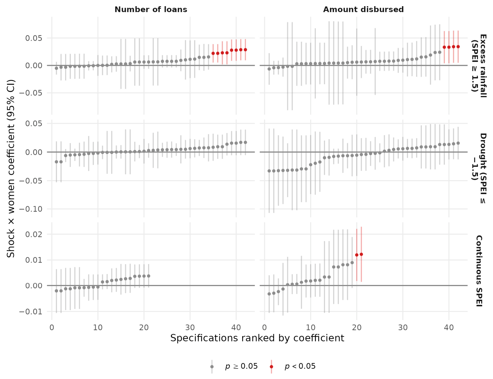
Figure A2.
Specification curve and specification matrix for the drought coefficients (42 specifications per outcome).
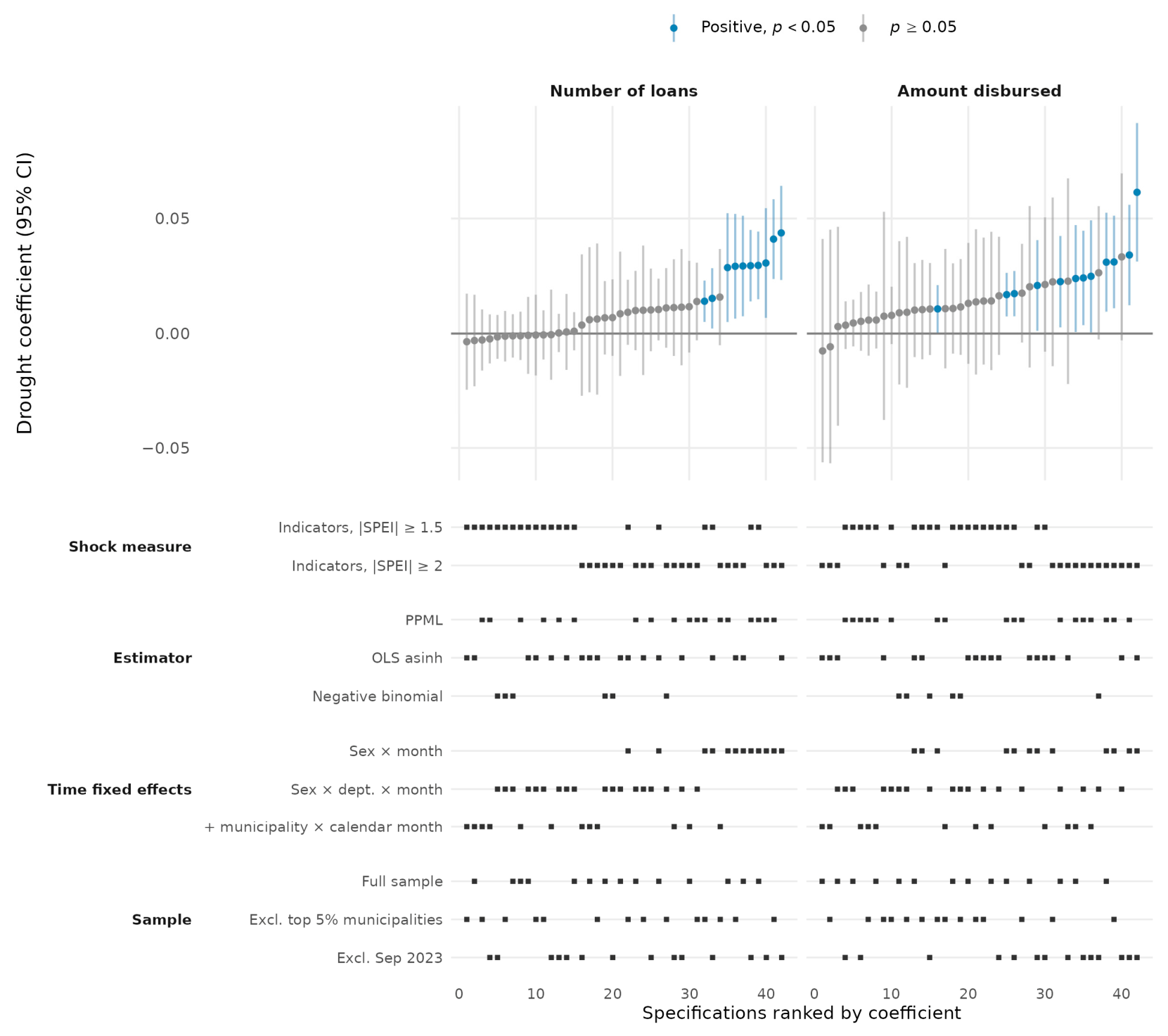
Figure A3.
Validation of the excess-rainfall indicator with precipitation-only measures and by intensity (PPML, preferred specification, 95% confidence intervals).
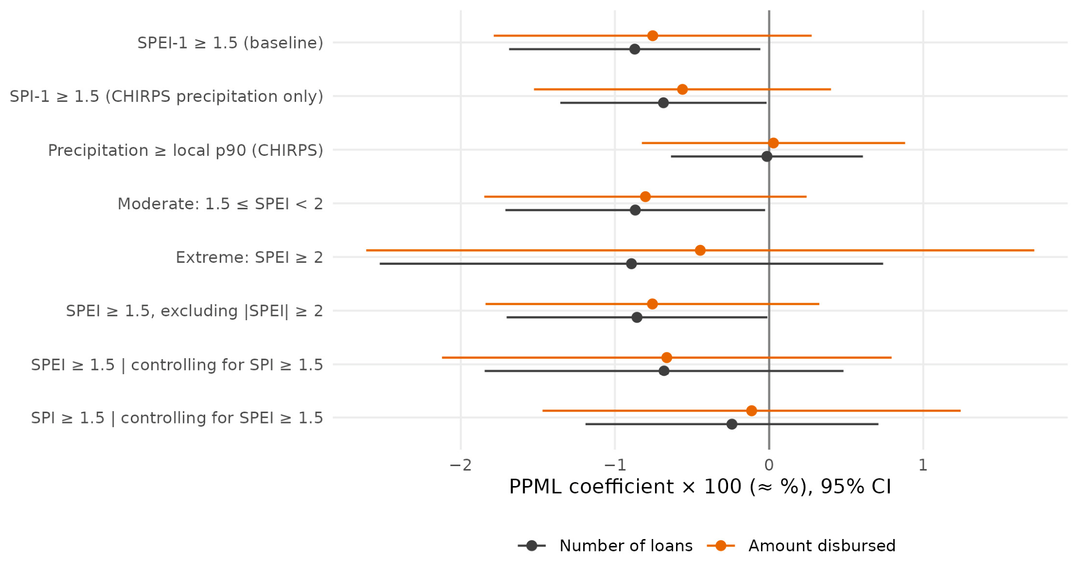
Table A1.
Within-lender design: full estimates.
Table A2.
Complete distributed-lag specifications.
Table A3.
Climate data diagnostics.
Table A4.
Agricultural exposure measured before the estimation period.
Table A5.
Estimators, market size, and aggregated counterfactual.
Table A6.
Official rurality classification (DNP) and comparison with the previous indicator.
Table A7.
Fixed versus random effects: Hausman and Mundlak tests.
References
- Morduch, J. Income Smoothing and Consumption Smoothing. J. Econ. Perspect. 1995, 9, 103–114. [Google Scholar] [CrossRef] [Scilit]
- Armendáriz, B.; Morduch, J. The Economics of Microfinance, 2nd ed.; MIT Press: Cambridge, MA, USA, 2010. [Google Scholar]
- Rios, D.; Perez, A.; Carabali, J.; Meneses, L.A.; Quiguanas, B. Market Power and Adverse Weather Events in a Market Dominated by Hydroelectric Energy. Estud. Gerenc. 2025, 41, 492–510. [Google Scholar] [CrossRef] [Scilit]
- Villa-Loaiza, C.; Taype-Huaman, I.; Benavides-Franco, J.; Buenaventura-Vera, G.; Carabalí-Mosquera, J. Does Climate Impact the Relationship between the Energy Price and the Stock Market? The Colombian Case. Appl. Energy 2023, 336, 120800. [Google Scholar] [CrossRef] [Scilit]
- Hoyos, N.; Escobar, J.; Restrepo, J.C.; Arango, A.M.; Ortiz, J.C. Impact of the 2010–2011 La Niña Phenomenon in Colombia, South America: The Human Toll of an Extreme Weather Event. Appl. Geogr. 2013, 39, 16–25. [Google Scholar] [CrossRef] [Scilit]
- Comisión Económica para América Latina y el Caribe (CEPAL). Valoración de Daños y Pérdidas: Ola Invernal en Colombia 2010–2011; CEPAL; Banco Interamericano de Desarrollo: Bogotá, Colombia, 2013. [Google Scholar]
- Kotz, M.; Levermann, A.; Wenz, L. The Effect of Rainfall Changes on Economic Production. Nature 2022, 601, 223–227. [Google Scholar] [CrossRef] [Scilit] [PubMed]
- Collier, B.; Katchova, A.L.; Skees, J.R. Loan Portfolio Performance and El Niño, an Intervention Analysis. Agric. Financ. Rev. 2011, 71, 98–119. [Google Scholar] [CrossRef] [Scilit]
- Aguilar-Gomez, S.; Gutierrez, E.; Heres, D.; Jaume, D.; Tobal, M. Thermal Stress and Financial Distress: Extreme Temperatures and Firms’ Loan Defaults in Mexico. J. Dev. Econ. 2024, 168, 103246. [Google Scholar] [CrossRef] [Scilit]
- Shoji, M. Does Contingent Repayment in Microfinance Help the Poor during Natural Disasters? J. Dev. Stud. 2010, 46, 191–210. [Google Scholar] [CrossRef] [Scilit]
- Khandker, S.R. Coping with Flood: Role of Institutions in Bangladesh. Agric. Econ. 2007, 36, 169–180. [Google Scholar] [CrossRef] [Scilit]
- Pelka, N.; Musshoff, O.; Weber, R. Does Weather Matter? How Rainfall Affects Credit Risk in Agricultural Microfinance. Agric. Financ. Rev. 2015, 75, 194–212. [Google Scholar] [CrossRef] [Scilit]
- Klomp, J. Do Natural Catastrophes Shake Microfinance Institutions? Using a New Measure of MFI Risk. Int. J. Disaster Risk Reduct. 2018, 27, 380–390. [Google Scholar] [CrossRef] [Scilit]
- Sseruyange, J.; Klomp, J. Natural Disasters and Economic Growth: The Mitigating Role of Microfinance Institutions. Sustainability 2021, 13, 5055. [Google Scholar] [CrossRef] [Scilit]
- Nie, O.; Regelink, M.; Wang, D. Banking Sector Risk in the Aftermath of Climate Change and Environmental-Related Natural Disasters; Policy Research Working Paper No. 10326; World Bank: Washington, DC, USA, 2023. [Google Scholar]
- Peters, V. How Banks are Impacted by and Mediate the Economic Consequences of Natural Disasters and Climate Shocks: A Review. De Econ. 2025, 173, 47–85. [Google Scholar] [CrossRef] [Scilit]
- Muñoz, J.; Pérez, A.; Carabali, J.; Buenaventura, G. Weather Shocks, Productivity, and Performance of Manufacturing Firms in Colombia. Empir. Econ. 2026, 70, 54. [Google Scholar] [CrossRef] [Scilit]
- Benavides Franco, J.; Carabali, J.A.; Meneses Cerón, L.Á.; Pérez, A.; Caicedo, Y.C. Weather Shocks and Banking Credit Risk: Evidence for Small Rural Municipalities in Colombia. Int. J. Financ. Stud. 2026, 14, 205. [Google Scholar] [CrossRef] [Scilit]
- Cortés, K.R.; Strahan, P.E. Tracing Out Capital Flows: How Financially Integrated Banks Respond to Natural Disasters. J. Financ. Econ. 2017, 125, 182–199. [Google Scholar] [CrossRef] [Scilit]
- Koetter, M.; Noth, F.; Rehbein, O. Borrowers under Water! Rare Disasters, Regional Banks, and Recovery Lending. J. Financ. Intermed. 2020, 43, 100811. [Google Scholar] [CrossRef] [Scilit]
- Brown, J.R.; Gustafson, M.T.; Ivanov, I.T. Weathering Cash Flow Shocks. J. Financ. 2021, 76, 1731–1772. [Google Scholar] [CrossRef] [Scilit]
- Noth, F.; Schüwer, U. Natural Disasters and Bank Stability: Evidence from the U.S. Financial System. J. Environ. Econ. Manag. 2023, 119, 102792. [Google Scholar] [CrossRef] [Scilit]
- Brei, M.; Mohan, P.; Perez Barahona, A.; Strobl, E. Transmission of Natural Disasters to the Banking Sector: Evidence from Thirty Years of Tropical Storms in the Caribbean. J. Int. Money Financ. 2024, 141, 103008. [Google Scholar] [CrossRef] [Scilit]
- Berg, G.; Schrader, J. Access to Credit, Natural Disasters, and Relationship Lending. J. Financ. Intermed. 2012, 21, 549–568. [Google Scholar] [CrossRef] [Scilit]
- Dorfleitner, G.; Forcella, D.; Gerckens, A. Climate Change in Microcredit Portfolios: Evidence on Vulnerability, Adaptation and Implications for Inclusive Finance. Bus. Strategy Environ. 2025, 34, 4409–4435. [Google Scholar] [CrossRef] [Scilit]
- Bohórquez-Peñuela, C.; Gáfaro, M.; Guzmán, K.; Pérez, A. Climate Risk and Access to Credit: Evidence from Colombian Potato Growers; Borradores de Economía No. 1307; Banco de la República: Bogotá, Colombia, 2025. [Google Scholar]
- Rodríguez-Novoa, D. Do Weather Shocks Affect Banks’ Loan Portfolio? Evidence from Colombia. Master’s Thesis, Universidad del Rosario, Bogotá, Colombia, 2022. [Google Scholar]
- de Roux, N. Exogenous Shocks, Credit Reports and Access to Credit: Evidence from Colombian Coffee Producers; Documento CEDE No. 2021-57; Universidad de los Andes: Bogotá, Colombia, 2021. [Google Scholar]
- Alesina, A.F.; Lotti, F.; Mistrulli, P.E. Do Women Pay More for Credit? Evidence from Italy. J. Eur. Econ. Assoc. 2013, 11, 45–66. [Google Scholar] [CrossRef] [Scilit]
- Bellucci, A.; Borisov, A.; Zazzaro, A. Does Gender Matter in Bank–Firm Relationships? Evidence from Small Business Lending. J. Bank. Financ. 2010, 34, 2968–2984. [Google Scholar] [CrossRef] [Scilit]
- Agier, I.; Szafarz, A. Microfinance and Gender: Is There a Glass Ceiling on Loan Size? World Dev. 2013, 42, 165–181. [Google Scholar] [CrossRef] [Scilit]
- Asfaw, S.; Maggio, G. Gender, Weather Shocks and Welfare: Evidence from Malawi. J. Dev. Stud. 2018, 54, 271–291. [Google Scholar] [CrossRef] [Scilit]
- Eastin, J. Climate Change and Gender Equality in Developing States. World Dev. 2018, 107, 289–305. [Google Scholar] [CrossRef] [Scilit]
- Auffhammer, M.; Hsiang, S.M.; Schlenker, W.; Sobel, A. Using Weather Data and Climate Model Output in Economic Analyses of Climate Change. Rev. Environ. Econ. Policy 2013, 7, 181–198. [Google Scholar] [CrossRef] [Scilit]
- Dell, M.; Jones, B.F.; Olken, B.A. What Do We Learn from the Weather? The New Climate–Economy Literature. J. Econ. Lit. 2014, 52, 740–798. [Google Scholar] [CrossRef] [Scilit]
- Damania, R.; Desbureaux, S.; Zaveri, E. Does Rainfall Matter for Economic Growth? Evidence from Global Sub-National Data (1990–2014). J. Environ. Econ. Manag. 2020, 102, 102335. [Google Scholar] [CrossRef] [Scilit]
- Garmaise, M.J.; Moskowitz, T.J. Catastrophic Risk and Credit Markets. J. Financ. 2009, 64, 657–707. [Google Scholar] [CrossRef] [Scilit]
- Petersen, M.A.; Rajan, R.G. The Benefits of Lending Relationships: Evidence from Small Business Data. J. Financ. 1994, 49, 3–37. [Google Scholar] [CrossRef]
- Jappelli, T.; Pagano, M. Information Sharing, Lending and Defaults: Cross-Country Evidence. J. Bank. Financ. 2002, 26, 2017–2045. [Google Scholar] [CrossRef] [Scilit]
- Karlan, D.; Osei, R.; Osei-Akoto, I.; Udry, C. Agricultural Decisions after Relaxing Credit and Risk Constraints. Q. J. Econ. 2014, 129, 597–652. [Google Scholar] [CrossRef] [Scilit]
- Demirgüç-Kunt, A.; Klapper, L.; Singer, D.; Ansar, S. The Global Findex Database 2021: Financial Inclusion, Digital Payments, and Resilience in the Age of COVID-19; World Bank: Washington, DC, USA, 2022; Available online: https://openknowledge.worldbank.org/handle/10986/37578 (accessed on 13 September 2026).
- Aterido, R.; Beck, T.; Iacovone, L. Access to Finance in Sub-Saharan Africa: Is There a Gender Gap? World Dev. 2013, 47, 102–120. [Google Scholar] [CrossRef] [Scilit]
- D’Espallier, B.; Guérin, I.; Mersland, R. Women and Repayment in Microfinance: A Global Analysis. World Dev. 2011, 39, 758–772. [Google Scholar] [CrossRef] [Scilit]
- de Mel, S.; McKenzie, D.; Woodruff, C. Are Women More Credit Constrained? Experimental Evidence on Gender and Microenterprise Returns. Am. Econ. J. Appl. Econ. 2009, 1, 1–32. [Google Scholar] [CrossRef] [Scilit]
- Carabalí, J.A.; Meneses Cerón, L.A.; Pérez Libreros, A.; Quiguanas, B.; Cabrera, D.; Guerrero, A.P. Weather Shocks and the Sugar–Ethanol Nexus in Colombia. Sustainability 2025, 17, 7125. [Google Scholar] [CrossRef] [Scilit]
- Castro, A.F.; Gómez Arteaga, N.; Llinás, G.; Mora, D.A. Definición de Categorías de Ruralidad; Archivos de Economía No. 437; Departamento Nacional de Planeación: Bogotá, Colombia, 2015.
- Wang, Q.; Yang, R.; Zhang, Y.; Yang, Y.; Hao, A.; Yin, Y.; Li, Y. Inequality of Carbon Emissions between Urban and Rural Residents in China and Emission Reduction Strategies: Evidence from Shandong Province. Front. Ecol. Evol. 2024, 12, 1256448. [Google Scholar] [CrossRef] [Scilit]
- Becchetti, L.; Castriota, S. Does Microfinance Work as a Recovery Tool after Disasters? Evidence from the 2004 Tsunami. World Dev. 2011, 39, 898–912. [Google Scholar] [CrossRef] [Scilit]
- Superintendencia Financiera de Colombia. Tasas de Interés Activas por Tipo de Crédito—Histórico [Dataset w9zh-vetq]. Datos Abiertos Colombia. Available online: https://www.datos.gov.co (accessed on 13 September 2026).
- Vicente-Serrano, S.M.; Beguería, S.; López-Moreno, J.I. A Multiscalar Drought Index Sensitive to Global Warming: The Standardized Precipitation Evapotranspiration Index. J. Clim. 2010, 23, 1696–1718. [Google Scholar] [CrossRef] [Scilit]
- Funk, C.; Peterson, P.; Landsfeld, M.; Pedreros, D.; Verdin, J.; Shukla, S.; Husak, G.; Rowland, J.; Harrison, L.; Hoell, A.; et al. The Climate Hazards Infrared Precipitation with Stations—A New Environmental Record for Monitoring Extremes. Sci. Data 2015, 2, 150066. [Google Scholar] [CrossRef] [Scilit] [PubMed]
- Muñoz-Sabater, J.; Dutra, E.; Agustí-Panareda, A.; Albergel, C.; Arduini, G.; Balsamo, G.; Boussetta, S.; Choulga, M.; Harrigan, S.; Hersbach, H.; et al. ERA5-Land: A State-of-the-Art Global Reanalysis Dataset for Land Applications. Earth Syst. Sci. Data 2021, 13, 4349–4383. [Google Scholar] [CrossRef] [Scilit]
- Departamento Administrativo Nacional de Estadística (DANE). Marco Geoestadístico Nacional: Municipios; DANE: Bogotá, Colombia, 2018. [Google Scholar]
- Thornthwaite, C.W. An Approach toward a Rational Classification of Climate. Geogr. Rev. 1948, 38, 55–94. [Google Scholar] [CrossRef] [Scilit] [PubMed]
- Beguería, S.; Vicente-Serrano, S.M.; Reig, F.; Latorre, B. Standardized Precipitation Evapotranspiration Index (SPEI) Revisited: Parameter Fitting, Evapotranspiration Models, Tools, Datasets and Drought Monitoring. Int. J. Climatol. 2014, 34, 3001–3023. [Google Scholar] [CrossRef] [Scilit]
- Santos Silva, J.M.C.; Tenreyro, S. The Log of Gravity. Rev. Econ. Stat. 2006, 88, 641–658. [Google Scholar] [CrossRef] [Scilit]
- Schmidheiny, K.; Siegloch, S. On Event Studies and Distributed-Lags in Two-Way Fixed Effects Models: Identification, Equivalence, and Generalization. J. Appl. Econom. 2023, 38, 695–713. [Google Scholar] [CrossRef] [Scilit]
- Khwaja, A.I.; Mian, A. Tracing the Impact of Bank Liquidity Shocks: Evidence from an Emerging Market. Am. Econ. Rev. 2008, 98, 1413–1442. [Google Scholar] [CrossRef] [Scilit]
- Hausman, J.A. Specification Tests in Econometrics. Econometrica 1978, 46, 1251–1271. [Google Scholar] [CrossRef] [Scilit]
- Mundlak, Y. On the Pooling of Time Series and Cross Section Data. Econometrica 1978, 46, 69–85. [Google Scholar] [CrossRef] [Scilit]
- Roth, J.; Sant’Anna, P.H.C.; Bilinski, A.; Poe, J. What’s Trending in Difference-in-Differences? A Synthesis of the Recent Econometrics Literature. J. Econom. 2023, 235, 2218–2244. [Google Scholar] [CrossRef] [Scilit]
- Jordà, Ò. Estimation and Inference of Impulse Responses by Local Projections. Am. Econ. Rev. 2005, 95, 161–182. [Google Scholar] [CrossRef] [Scilit]
- Abadie, A.; Athey, S.; Imbens, G.W.; Wooldridge, J.M. When Should You Adjust Standard Errors for Clustering? Q. J. Econ. 2023, 138, 1–35. [Google Scholar] [CrossRef] [Scilit]
- Barrios, T.; Diamond, R.; Imbens, G.W.; Kolesár, M. Clustering, Spatial Correlations, and Randomization Inference. J. Am. Stat. Assoc. 2012, 107, 578–591. [Google Scholar] [CrossRef] [Scilit]
- Conley, T.G. GMM Estimation with Cross Sectional Dependence. J. Econom. 1999, 92, 1–45. [Google Scholar] [CrossRef] [Scilit]
- Driscoll, J.C.; Kraay, A.C. Consistent Covariance Matrix Estimation with Spatially Dependent Panel Data. Rev. Econ. Stat. 1998, 80, 549–560. [Google Scholar] [CrossRef] [Scilit]
- Steegen, S.; Tuerlinckx, F.; Gelman, A.; Vanpaemel, W. Increasing Transparency Through a Multiverse Analysis. Perspect. Psychol. Sci. 2016, 11, 702–712. [Google Scholar] [CrossRef] [Scilit] [PubMed]
- Holm, S. A Simple Sequentially Rejective Multiple Test Procedure. Scand. J. Stat. 1979, 6, 65–70. [Google Scholar]
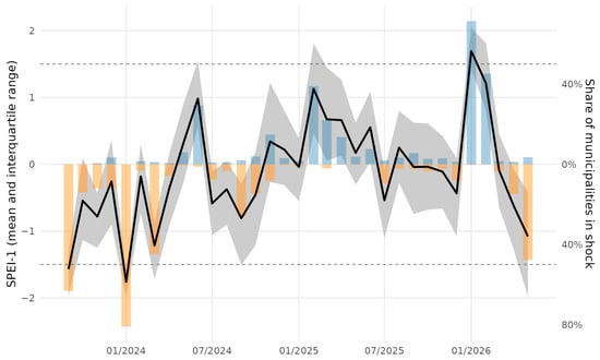
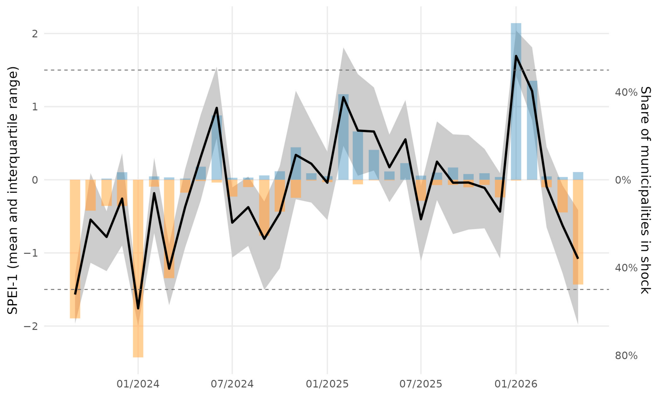
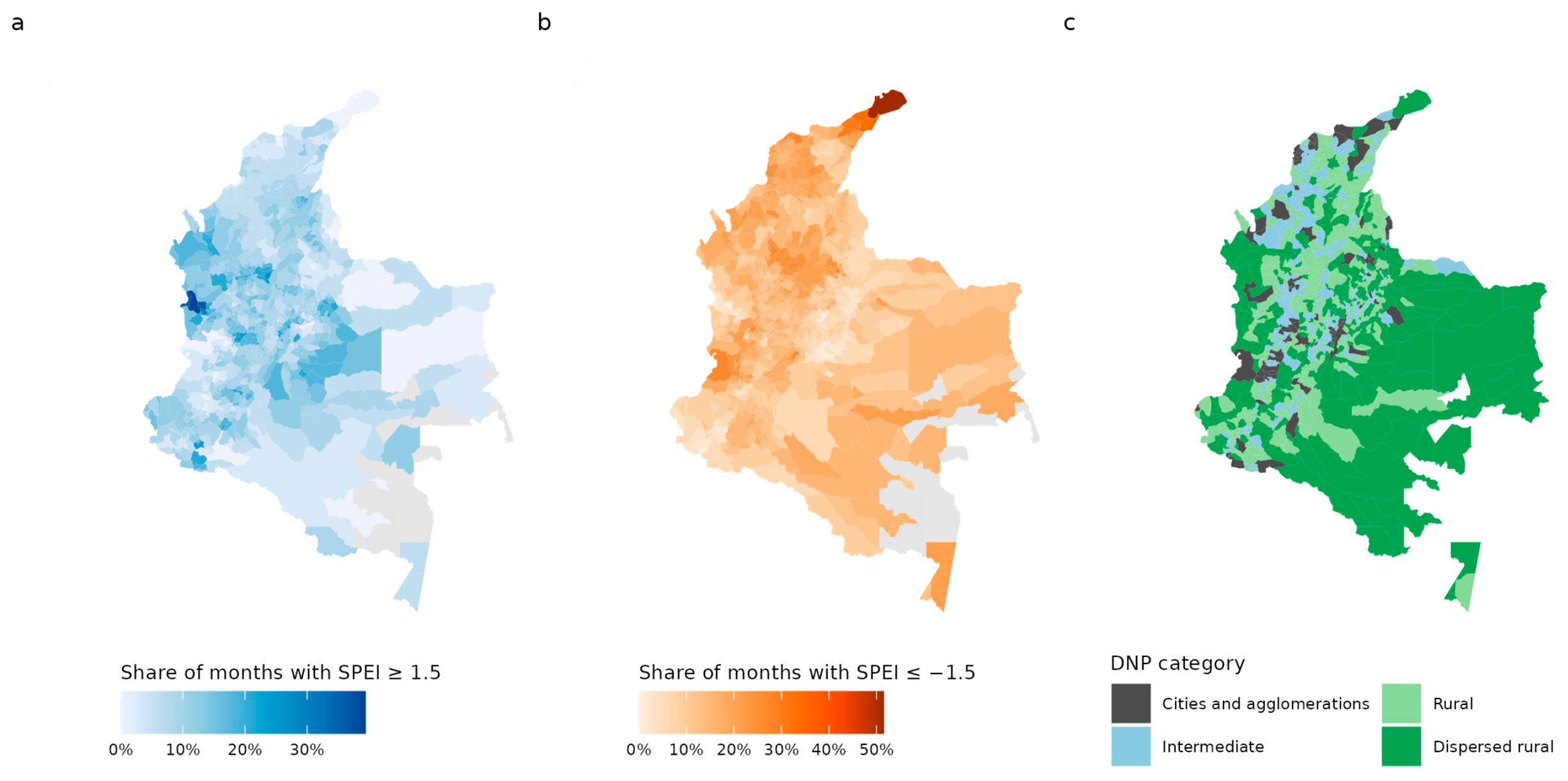
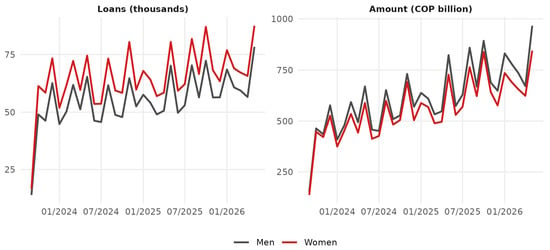
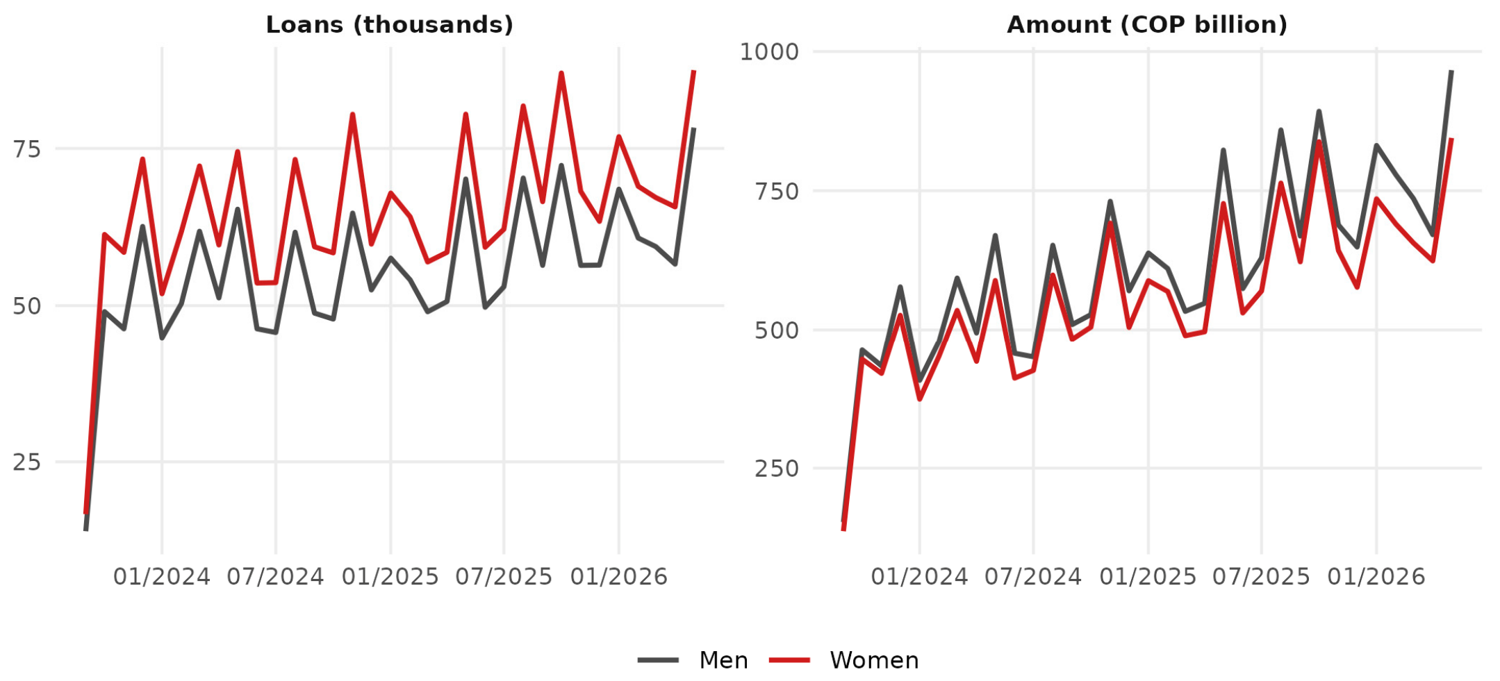
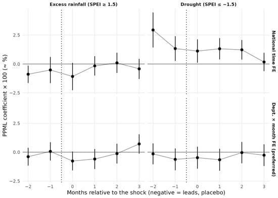
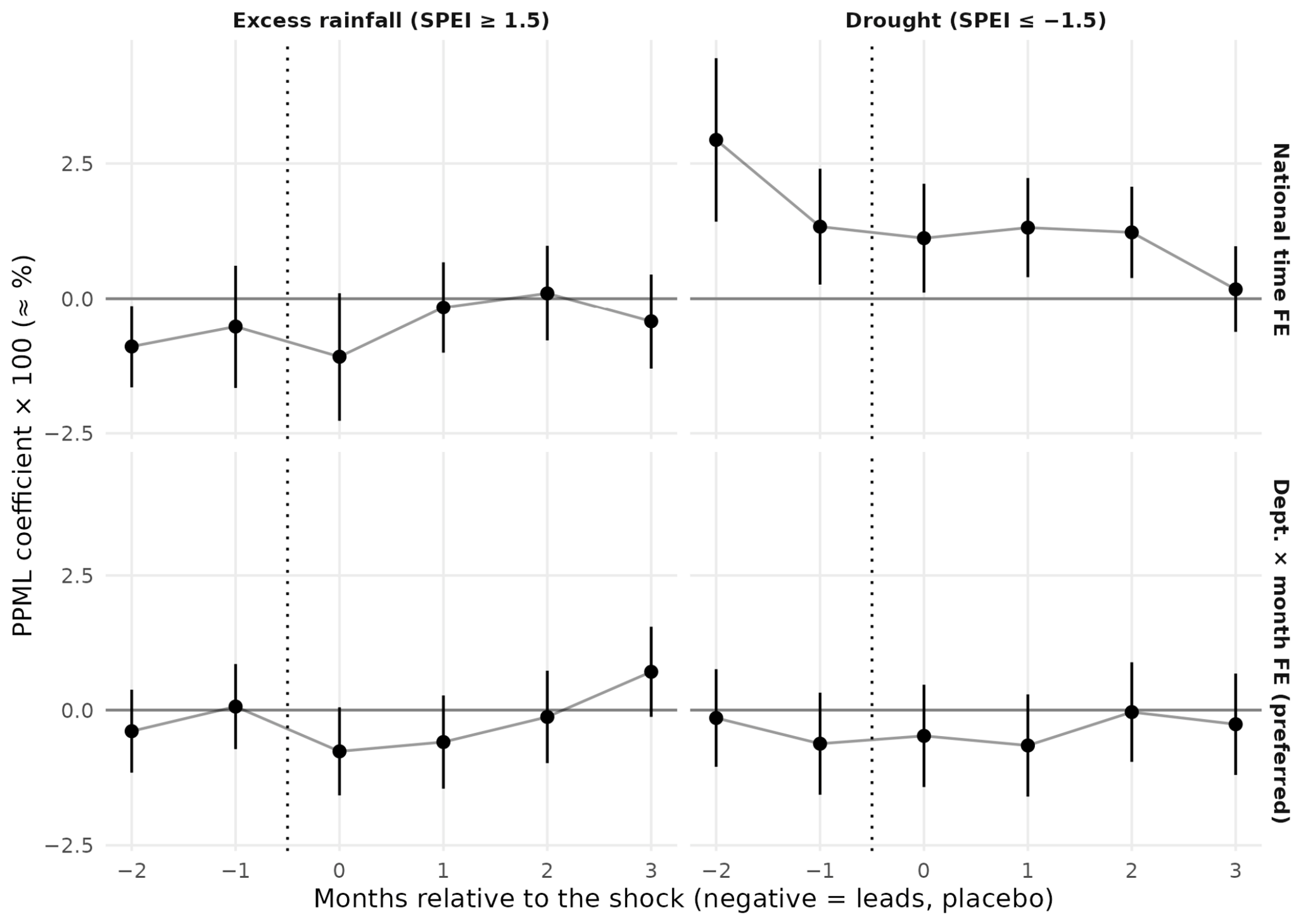
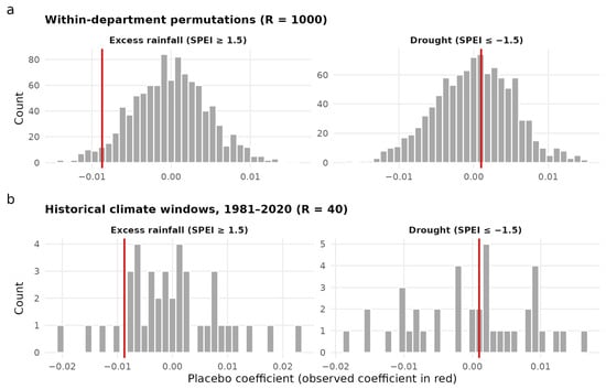
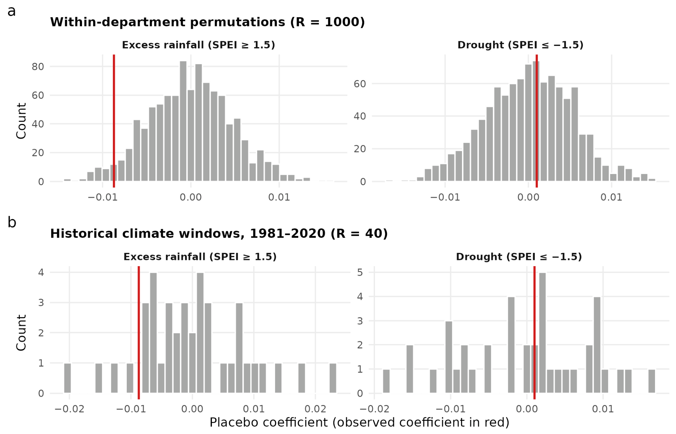
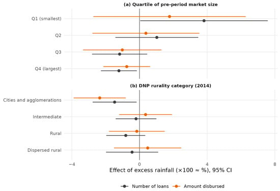
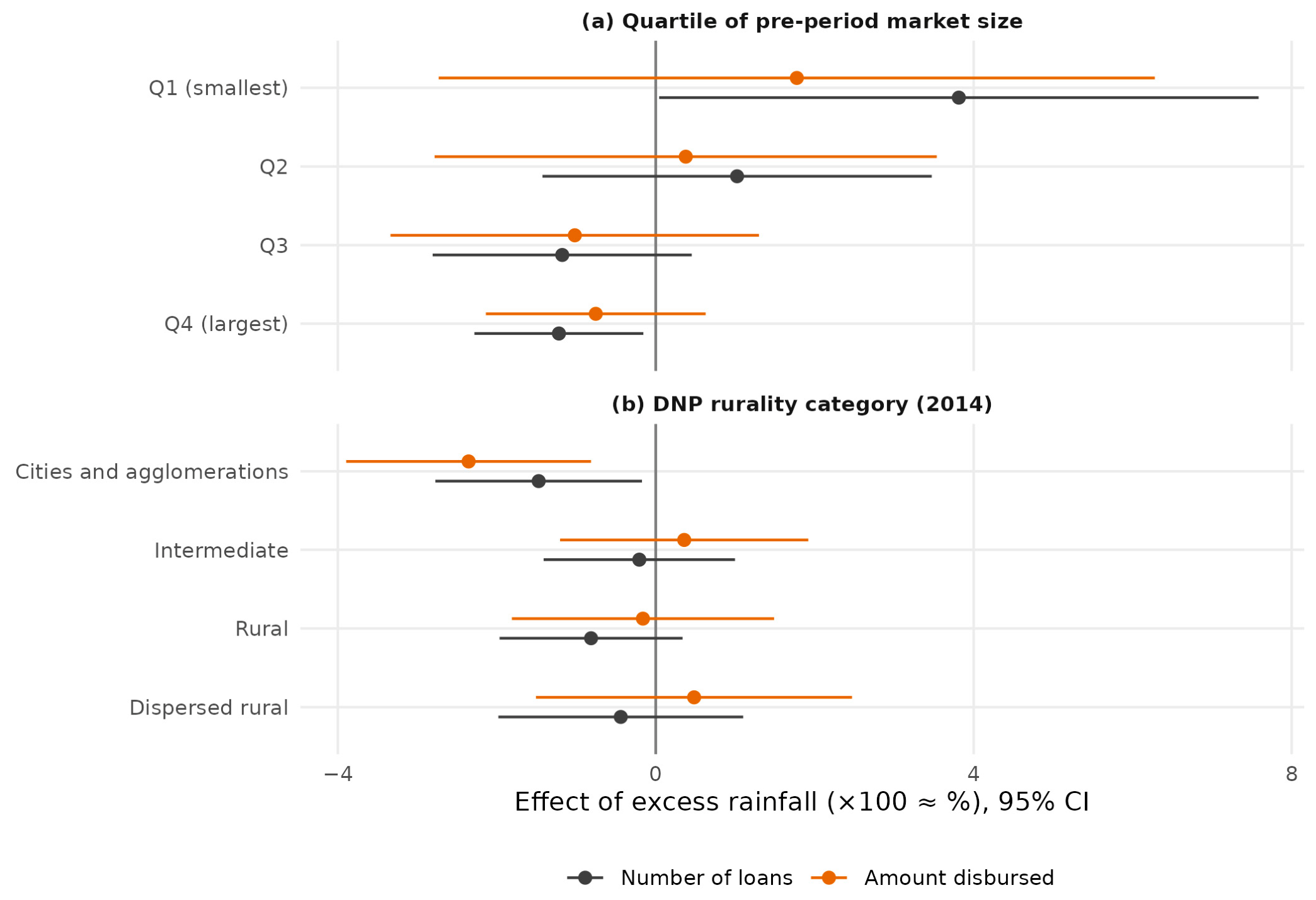
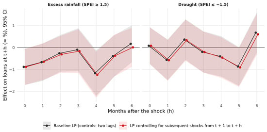
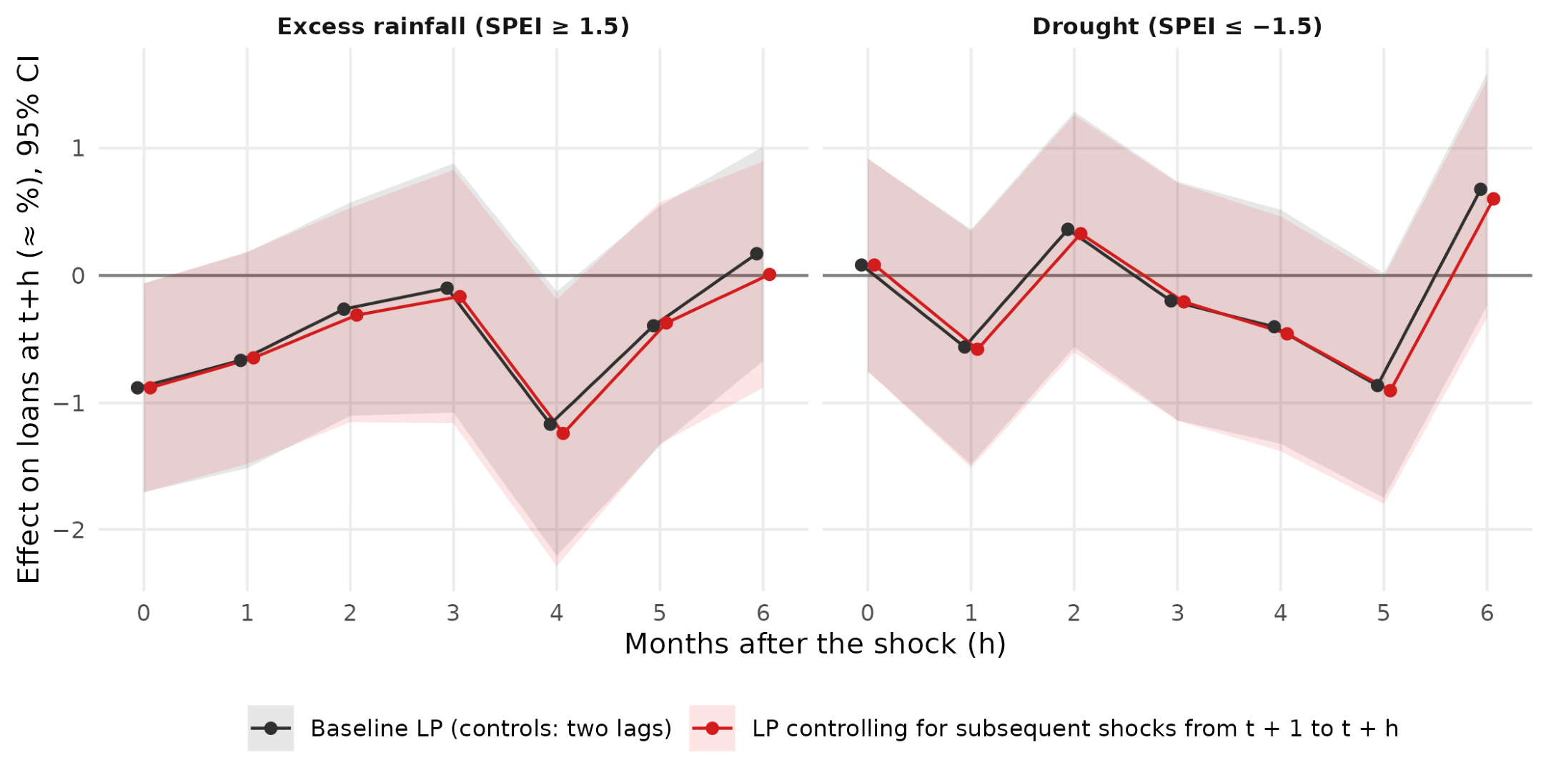
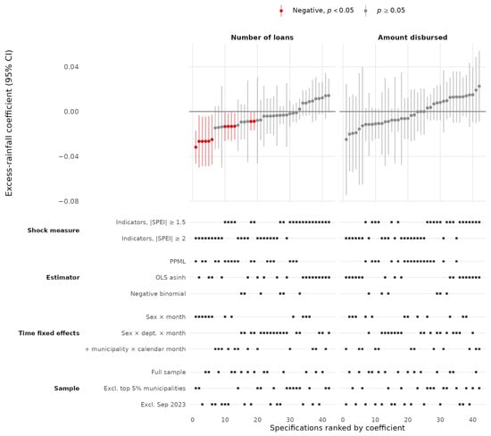
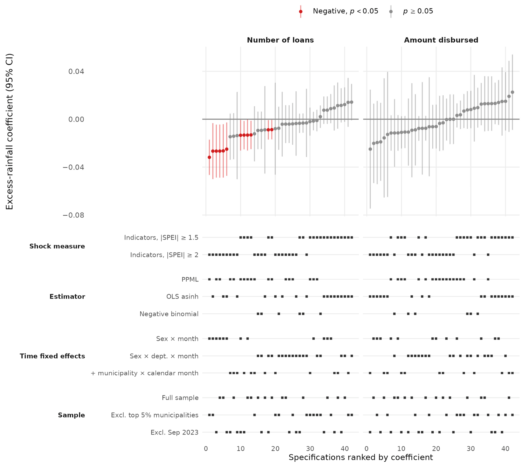
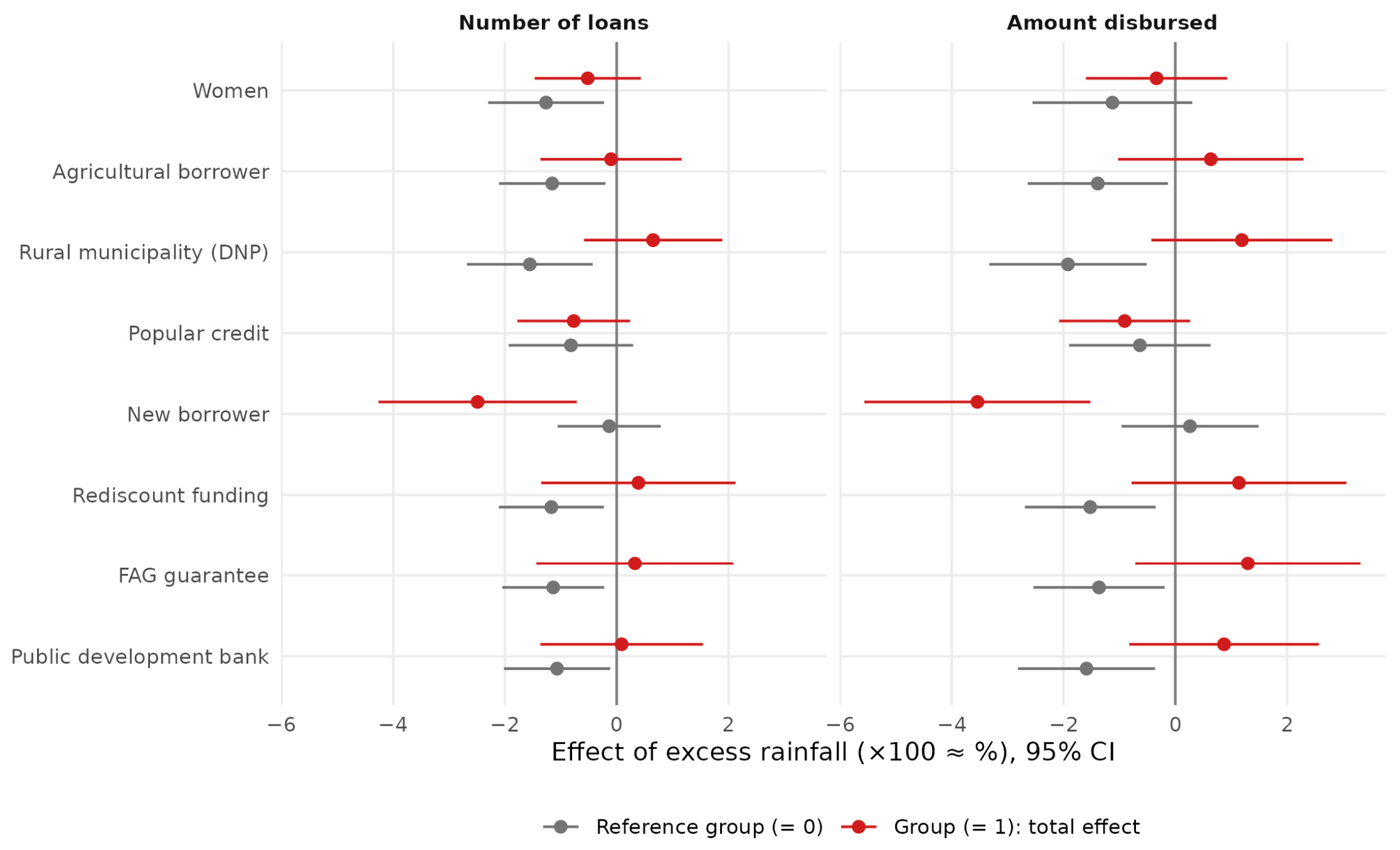

Disclaimer/Publisher’s Note: The statements, opinions and data contained in all publications are solely those of the individual author(s) and contributor(s) and not of MDPI and/or the editor(s). MDPI and/or the editor(s) disclaim responsibility for any injury to people or property resulting from any ideas, methods, instructions or products referred to in the content. |
© 2026 by the authors. Licensee MDPI, Basel, Switzerland. This article is an open access article distributed under the terms and conditions of the Creative Commons Attribution (CC BY) license.