Three-Dimensional Coupling Assessment of Eco-Geological Environment in Alpine Gorge Areas Integrating the Remote Sensing Ecological Index, Ecosystem Services, and Geological Environment Carrying Capacity

Abstract

Alpine gorge areas are typical regions where ecological fragility and geological hazard risk overlap strongly. Existing eco-geological assessments remain largely single- or dual-dimensional: remotely sensed indices describe surface status, ecosystem-service indices describe functional supply, and geological models are usually applied separately from ecological assessment, so each approach misses the information carried by the others. To close this gap, this study proposes a three-dimensional coupling framework for Eco-Geological Environment Carrying Capacity (EGECC) that integrates the Remote Sensing Ecological Index (RSEI), the Ecosystem Services Index (ESI) and the Geological Environmental Carrying Capacity (GECC), and applies it in Lixian County, Sichuan Province. The three indices were coupled at pixel level, and their coupling and vertical differentiation were analysed along an altitudinal gradient. Three findings are highlighted. (1) RSEI and ESI are only moderately correlated, and their altitudinal peaks are separated, so neither can substitute for the other. (2) GECC contributes the largest share of the variation in EGECC, indicating that the geological dimension carries information that is not a linear combination of the two ecological dimensions. (3) Consequently, the geological dimension cannot be reproduced from the ecological ones: degrading the framework to RSEI + ESI places part of the area in a lower class that the two-dimensional scheme would label as safe. A five-tier management strategy is outlined accordingly. The study provides a transferable basis for eco-geological zoning in alpine gorge counties.

1. Introduction

Eco-geological environment quality assessment is a fundamental task for regional territorial spatial planning and ecological security pattern construction, directly related to the achievement of regional sustainable development goals and the scientific delineation of ecological protection red lines [1,2]. With the continuous intensification of human activities and global climate change, issues such as ecosystem degradation, frequent geological disasters, and declining environmental carrying capacity are increasingly intertwined. The assessment objects of eco-geological environments have gradually expanded from single ecological or geological elements to composite systems encompassing surface status, service functions, and geological risks [3,4]. How to scientifically and comprehensively evaluate regional eco-geological environment quality has become a core topic in environmental science and geoscience. Alpine gorge areas, characterised by intense tectonic activity, dramatic topographic relief, and highly overlapping ecological and geological risks, have become challenging and focal regions for eco-geological environment assessment [5,6]. However, current eco-geological environment assessments mostly focus on single-dimensional or dual-dimensional evaluation; therefore, there is an urgent need to construct a three-dimensional coupling assessment framework that integrates surface status, service functions, and geological risks.

The Remote Sensing Ecological Index (RSEI) aggregates four remotely sensed ecological indicators—greenness (NDVI), wetness (WET), heat (LST) and dryness (NDBSI)—through Principal Component Analysis (PCA), using the variance contribution of the first principal component (PC1) as the integration weight, and it has been widely applied in regional ecological quality assessment [7,8,9]. Because all four components are derived from surface spectral and thermal radiation signals received by satellite sensors [10], RSEI essentially characterises the physical state of the land surface.

Ecosystem services (ESs) are the conditions and benefits that ecosystems provide for human well-being [11,12], and carbon sequestration, water conservation, soil conservation and wind–sand control are widely used indicators of their regulating capacity [13,14]. Although RSEI and the Ecosystem Services Index (ESI) are both used as measures of ecological quality, they capture different dimensions: RSEI describes physical surface features such as vegetation cover and surface temperature–moisture conditions, whereas ESI quantifies ecological processes such as carbon sequestration and water conservation, and the two do not necessarily agree in space [11]. In alpine gorge areas, this divergence is amplified, because a geological disaster can destroy the service base of a high-RSEI area almost instantly [15], so that evaluating either dimension alone is likely to misjudge the actual security pattern.

The Geological Environmental Carrying Capacity (GECC) integrates lithology, fault structure and topographic relief to describe the support and constraints that the geological environment imposes on ecosystems, and it supplies the geological dimension that neither RSEI nor ESI contains [16,17]. The three are not independent: under the same geological baseline, dense vegetation and strong soil conservation suppress slope erosion and shallow landslides and thus raise the effective safety margin, whereas vegetation degradation and the loss of service functions expose the vulnerability of that baseline [18,19]. RSEI, ESI and GECC therefore each capture a different dimension of the eco-geological environment and each has its own information blind spot, and in alpine gorge areas the high heterogeneity of the geological environment makes this particularly consequential: ecological assessment without geological constraint and geological assessment without ecological feedback are equally one-sided. To the best of our knowledge, however, no existing framework has assessed the three synergistically in a single three-dimensional system, and this gap is most consequential in alpine gorge areas where ecological protection and geological hazard prevention are equally urgent. Filling it is the purpose of this study.

On this basis, this study proposes the EGECC three-dimensional coupling framework and applies it in Lixian County, Sichuan Province, in order to answer three questions: (1) To what extent do RSEI and ESI agree in space, and where do they couple and decouple? (2) Does the geological dimension carry information that cannot be reproduced by any combination of the two ecological dimensions? (3) How do the three dimensions covary along the altitudinal gradient, and what does this imply for vertically differentiated management? To answer them, RSEI, ESI and GECC were computed on a common analysis grid resampled from the 30 m source data, coupled at grid-cell level through cross-coupling matrices and an equal-weight overlay, and profiled along the altitude gradient; the predictive performance of the GECC model was re-examined with spatial cross-validation. The remainder of the paper is organised as follows: Section 2 describes the study area, the data and the four component methods; Section 3 reports the results; Section 4 discusses the coupling mechanisms, the management implications and the limitations; and Section 5 concludes.

2. Materials and Methods

2.1. Study Area

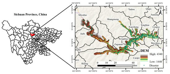
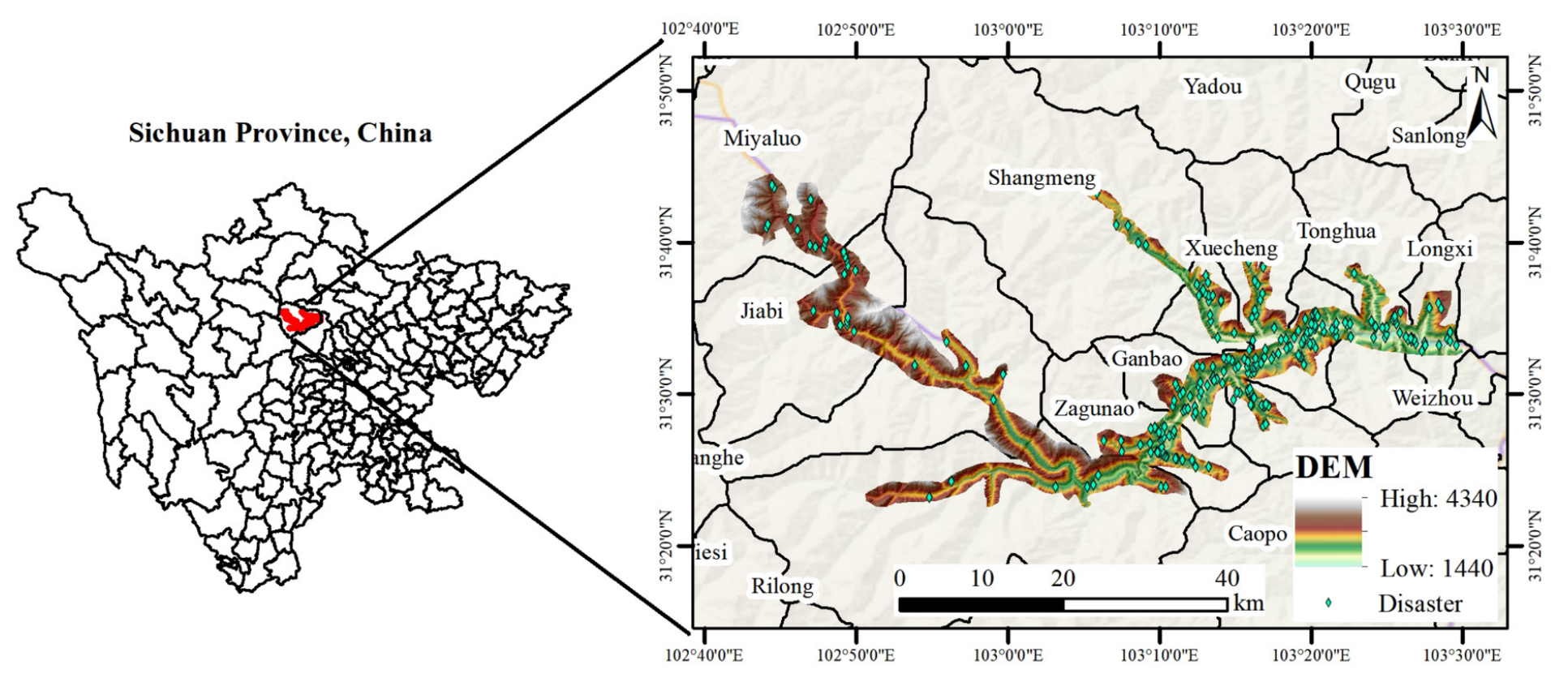
Lixian County is located in northwestern Sichuan Province, on the northeastern margin of the Qinghai–Tibet Plateau (102.55–103.50° E, 31.20–31.85° N), situated in the transition zone between the northern Hengduan Mountains and the western Sichuan alpine gorge area, under the jurisdiction of Aba Tibetan and Qiang Autonomous Prefecture, with a total area of approximately 4318 km² (Figure 1). The study area has a topography that is high in the northwest and low in the southeast, with elevations ranging from 1440 to 4340 m and a relative elevation difference of about 2900 m, representing typical alpine gorge landforms. The climate belongs to the plateau monsoon type, jointly controlled by the southeast monsoon and the large-scale terrain of the Qinghai–Tibet Plateau, with significant vertical differentiation. Precipitation is concentrated from May to September, and torrential rainfall is the key meteorological factor triggering geological disasters. The tectonic setting is located at the intersection of the Songpan–Garze Fold Belt and the Longmenshan Fault Zone, with the Minjiang Fault Zone, the Huya Fault Zone, and the back-mountain fault of the Longmenshan Fault Zone traversing the entire area. Tectonic activity is intense, and geological disasters such as landslides, rockfalls, and debris flows occur frequently. Vegetation types encompass a complete vertical zonal spectrum from arid valley shrublands to sparse scree vegetation, with rich ecosystem types and distinct gradient differentiation. Lixian County can be taken as representative of the alpine gorge environments of the eastern margin of the Qinghai–Tibet Plateau: within 4318 km² it combines a relief amplitude of about 2900 m, an active fault network at the junction of the Songpan–Garze Fold Belt and the Longmenshan Fault Zone, and a complete vegetation spectrum from arid-valley shrubland to alpine scree, so that ecological gradients, geological hazard processes and human settlement are compressed into a single county that can be mapped at a 30 m resolution. The same combination of conditions recurs throughout the Hengduan Mountains and the western Sichuan alpine gorge region [5,6].

Figure 1. Location map of the study area (DEM elevation range: 1440–4340 m).

2.2. Data Sources and Preprocessing

The data used in this study include remote sensing imagery, a Digital Elevation Model (DEM), geological and environmental factor data, and historical disaster point data. Remote sensing imagery was acquired from Landsat 8 OLI/TIRS images (spatial resolution: 30 m), which were acquired in the vegetation growing season (July–September) with cloud cover below 10%, and all were from 2020. After radiometric calibration, atmospheric correction (FLAASH), and geometric precision correction, the images were used for RSEI calculation. The Copernicus DEM GLO-30 (30 m) was used to extract terrain factors, including elevation, slope, aspect, curvature, valley depth, relief, slope shape, Terrain Ruggedness Index (TRI), and Topographic Wetness Index (TWI). Geological data included 1:200,000 regional geological maps (stratum lithology and fault structures), which were vectorised and rasterised to a 30 m resolution. Linear features such as roads and rivers were extracted from OpenStreetMap, and Euclidean distance analysis was used to generate spatial distance factors, including distance to fault, distance to road, and distance to river. The historical disaster points (landslides, rockfalls and debris flows) were identified from 2020 UAV optical imagery and confirmed by field survey. All data were uniformly projected to the WGS 1984 UTM Zone 48N coordinate system and resampled to a 30 m raster resolution. The river and road vectors used to construct the distance factors were extracted from OpenStreetMap; the county boundary and the settlement locations shown in the figures serve only to delimit the study area and to describe the exposure of elements at risk in Section 4.4 and are not inputs to RSEI, ESI or GECC, so their positional accuracy does not affect the index values. Because every input is evaluated on 30 m cells, any residual georeferencing error in these vector layers is bounded by one cell and is not propagated into the results. The three groups of input data do not share an identical temporal reference: the Landsat 8 scenes and the historical disaster points are both from 2020, whereas the Copernicus DEM is a static product with no acquisition date. Because lithology, fault structure and terrain change slowly relative to these intervals, the three layers are treated as contemporaneous; the residual mismatch and its consequences are discussed in Section 4.5. The elevation range of the study area derived from the DEM is 1440–4340 m. All data have a spatial resolution of 30 m; after processing and fusion, the raster dataset comprises 64,532 cells, on which all subsequent analyses were carried out.

2.3. RSEI Evaluation Method

The Remote Sensing Ecological Index (RSEI) is a comprehensive regional ecological environment quality assessment model entirely based on remote sensing imagery without the need for artificially assigned weights. RSEI selects four ecological indicators closely related to human perception—greenness, wetness, heat, and dryness—and integrates them through Principal Component Analysis (PCA). Specifically, the greenness indicator uses the Normalised Difference Vegetation Index (NDVI) to reflect surface vegetation cover and growth status [20]; the wetness indicator is represented by the third component of tasselled cap transformation (WET), using linear combinations of band reflectances to reflect the moisture content of surface soil and vegetation [21]; the dryness indicator is synthesised by averaging the Bare Soil Index (SI) and Index-Based Built-Up Index (IBI) to form NDBSI, characterising surface bare soil and built-up land conditions [22]; the heat indicator uses Land Surface Temperature (LST), obtained from thermal infrared bands through radiometric calibration, brightness temperature calculation, and land surface emissivity correction, to reflect the surface thermal environment distribution [23]. Before PCA the four indicators were min–max normalised to [0, 1]; PC1 accounted for 65.74 of the total variance (eigenvalue: 2.630), and the loadings of NDVI, WET, LST and NDBSI on PC1 were +0.474 (NDVI), +0.494 (WET), −0.538 (LST) and −0.492 (NDBSI), with the signs indicating that PC1 increases with greenness and wetness and decreases with heat and dryness; the PCA results are summarised in Table 1. The resulting PC1 was again min–max normalised to [0, 1] to give RSEI.

Table 1. Principal component analysis of the RSEI and ESI indicator sets.

Index Set	Eigenvalue of PC1	Variance Explained by PC1 (%)	Eigenvalue of PC2	Variance Explained by PC2 (%)	Loadings on PC1 (in the Order Given in the Text)
RSEI (NDVI, WET, LST, NDBSI)	2.630	65.74	0.666	16.64	+0.474/+0.494/−0.538/−0.492
ESI (NPP, WY, SC, WSC)	1.823	45.57	0.990	24.75	+0.644/+0.655/−0.120/−0.377

Note: PC1 is the component used to build each index; the loadings are given with their sign.

2.4. ESI Evaluation Method

The Ecosystem Services Index (ESI) aims to compensate for the limitation of RSEI, which relies solely on surface indicators and cannot comprehensively reflect the evolution trends of ecosystem service functions [11]. ESI selects multiple ecosystem service indicators closely related to regional ecological benefits and adopts the same PCA integration framework as RSEI for comprehensive assessment, enabling quantitative characterisation of the overall supply capacity of regional ecosystem services [12]. Considering the mountain–valley geomorphological characteristics of Lixian County and data availability, this study selects four ecosystem service indicators—Net Primary Productivity (NPP), water yield (WY), soil conservation (SC), and wind–sand control (WSC)—to construct the ESI. All four indicators were taken directly from publicly available raster datasets at a 30 m resolution rather than computed in this study: NPP from the 2020 annual national terrestrial NPP raster dataset (NPP2020) and water yield, soil conservation and wind–sand control from published raster products, which were used as provided, without re-running the InVEST or RWEQ models; the parameterisation is therefore that of the published products. All four indicators were min–max normalised to [0, 1] and integrated by PCA; PC1 accounted for 45.57 of the variance with loadings +0.644 (NPP), +0.655 (WY), −0.120 (SC) and −0.377 (WSC) (Table 1). Because WSC has the lowest mean and the weakest loading, ESI was also recomputed without it: the resulting ESI differed from the four-indicator version by a Pearson r of 0.963 with the four-indicator version, with 17.7% of the area changing class, so WSC was retained as an indicator of the wind-erosion regulation service despite its small local contribution.

2.5. GECC Evaluation Method

This study selected 15 categories of geological environment factors to construct the GECC assessment indicator system, covering three major categories: terrain factors (12 items, including elevation, slope, aspect, curvature, profile curvature, plan curvature, valley depth, relief, slope shape, Terrain Ruggedness Index (TRI), distance to river, and Topographic Wetness Index (TWI)); geological factors (2 items: stratum lithology and distance to fault); and human activity factors (1 item: distance to road) [24,25,26]. The 286 historical disaster points (landslides, rockfalls and debris flows, identified from 2020 UAV optical imagery and confirmed by field survey) served as positive samples; because a binary classifier also requires negatives, non-disaster (background) samples (284) were generated by random sampling of locations away from the recorded disaster points at an approximately 1:1 ratio, which was chosen to avoid class imbalance in the training set. A Random Forest (RF) model was employed for Geological Environmental Carrying Capacity assessment. RF is an ensemble learning algorithm based on the Bagging strategy, which improves prediction accuracy and anti-overfitting capability by constructing multiple decision trees and voting ensemble [27]. Its core hyperparameters (ntree and mtry) were fixed at ntree = 500, mtry = sqrt(p) with p = 15 (i.e., three to four predictors per split), balanced class weights and the random seed fixed at 42. Model accuracy was evaluated using AUC [28]; to separate the optimistic bias that random splitting of spatial data can produce, the sample was additionally partitioned by 5 km × 5 km spatial blocks, which gave 45 blocks, and these were combined into five folds and the model was refitted. It should be noted that the RF is trained on the presence or absence of past disasters and is therefore, strictly, a model of the spatial susceptibility of the terrain to geological hazards; we define GECC as the complement of the modelled hazard probability, on the assumption that a location where the carrying capacity has not been exceeded during the recorded period retains a higher residual carrying capacity. The background sample is drawn at random from locations away from the recorded disaster points rather than from an inventory of confirmed safe sites, so it represents the non-failure condition on which the definition of GECC relies; the interpretation of GECC as residual carrying capacity is therefore conditional on the completeness of the inventory, as stated in Section 4.5. GECC is thus a model-derived index of the relative ability of the geological environment to sustain ecological and human use without failure. Higher GECC values therefore denote more favourable conditions, i.e., a higher residual carrying capacity; the index is not itself a hazard probability, and the EGECC classes are reported throughout in terms of carrying capacity rather than risk. The 2 km, 500 m and 1–3 km distances used to describe the low- and moderate-GECC belts are interpretive thresholds rather than model parameters; they follow the frequency ratio of inventoried disaster points to area as a function of distance to the nearest fault, which falls from 2.03 within 500 m to about 1.0 at 1.0–1.5 km and to 0.3–0.4 beyond 4 km, so that 1–3 km brackets the distance at which the fault-proximity effect ceases to be detectable in the inventory. Varying these thresholds by ±50% changed the area shares of the belts by less than 9.1 percentage points.

2.6. EGECC Three-Dimensional Coupling Framework, Equal-Weight Justification and Analysis Method

The three sets of raster data—RSEI, ESI, and GECC—were spatially overlaid to achieve raster-level quantitative coupling, constructing the EGECC three-dimensional assessment framework. The coupling analysis includes the following steps: first, RSEI, ESI, and GECC were each classified into three levels—Low (1), Medium (2), and High (3)—using the natural-breaks method (Jenks); second, the EGECC composite score was constructed through equal-weight linear overlay: EGECC = RSEIlevel + ESIlevel + GECClevel; finally, the EGECC scores were classified into four comprehensive levels—Low, Moderate, High, and Extremely High—using the natural-breaks method (Jenks), and the area proportion of each level was calculated. All spatial analyses and statistical calculations were performed in ArcGIS 10.8 and Python 3 with the scikit-learn, NumPy and pandas libraries.

Justification of the equal weights. Equal weights were adopted because the three dimensions are meant to enter the framework as independent, non-substitutable information layers rather than as competing predictors of one quantity: each answers a different question (what the surface looks like, what it supplies, whether it may fail), and there is no external reference variable against which their relative importance for eco-geological security could be calibrated. Equal weighting is also the most transparent and reproducible choice and avoids presenting a subjective judgement as a measurement.

Analysis units and spatial autocorrelation. The source data have a spatial resolution of 30 m; for the coupled assessment, the indicator rasters were resampled to a regular analysis grid of approximately 250 m, and the 64,532 cells inside the county boundary form the analysis set that covers the 4318 km² study area; the effective cell area implied by the cell count and the county area is 66,915 m², or about 259 m on a side, the difference from the nominal cell size reflecting boundary cells clipped by the irregular county outline. The 30 m figure refers to the source data only, not to the analysis cells, and all subsequent analyses were carried out on these analysis cells. Because neighbouring cells are spatially autocorrelated, the nominal n overstates the number of independent observations; the correlations are therefore reported as descriptive statistics and are not used for significance testing.

3. Results

3.1. RSEI Results Analysis

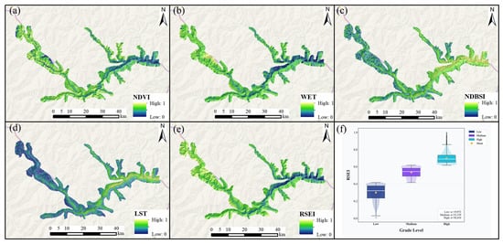
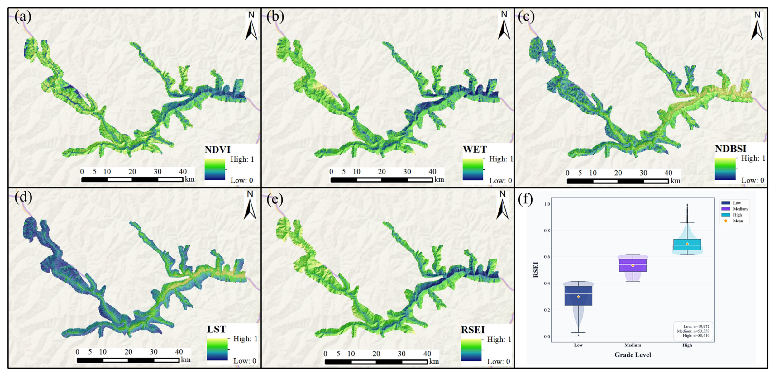
As shown in Figure 2, high RSEI values are concentrated in the high-altitude plateau areas in the northern part of the study area, where the terrain is gentle and open, dominated by alpine meadows and wetland marshes with high vegetation cover and good ecosystem integrity; low RSEI values mainly appear in the deeply incised valley areas in the eastern part of the study area, where sparse vegetation at the valley bottom, combined with disturbance from human engineering activities, leads to evident habitat degradation. Among the four components, NDVI is highest on the northern high mountains and in the central–western primary forest and lowest in the east, where vegetation cover is reduced by human activity; WET is higher in the east than in the west, reflecting the humid regional climate; NDBSI is high only over built-up areas, highway corridors and valley bare-rock belts, and low wherever a closed forest canopy is present; and LST is highest in the valley bottoms and low-altitude settlements and lowest on the high mountains and snow-covered areas. These patterns follow directly from Figure 2 and are summarised rather than described in detail.

Figure 2. RSEI indicators and results. (a) NDVI; (b) WET; (c) NDBSI; (d) LST; (e) RSEI; (f) RSEI at different grades.

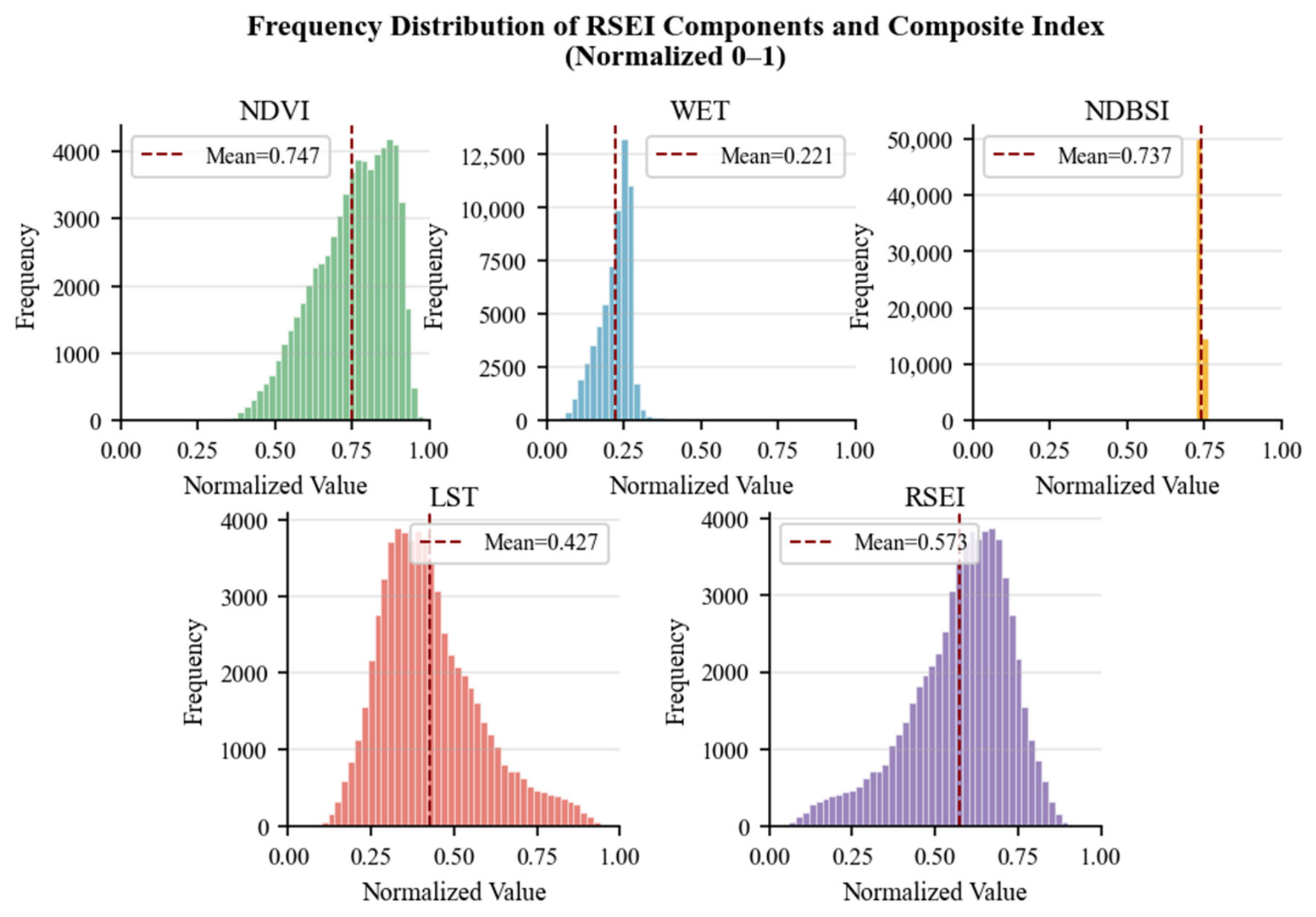
Figure 3 shows the frequency distributions of RSEI and its four components after normalisation. RSEI is near-normally distributed with a mean of 0.573, indicating a moderately good ecological level overall; NDVI has the highest mean (0.747) and is concentrated in the mid-to-high range; WET (0.221) is right-skewed with a right tail of locally humid habitats; NDBSI has an extremely narrow distribution, indicating that dryness varies little across the county; and LST is right-skewed and weakly bimodal, consistent with its negative relationship with elevation. The PCA on which RSEI is based is reported in Table 1.

Figure 3. Frequency distribution of RSEI components and composite index.

3.2. ESI Results Analysis

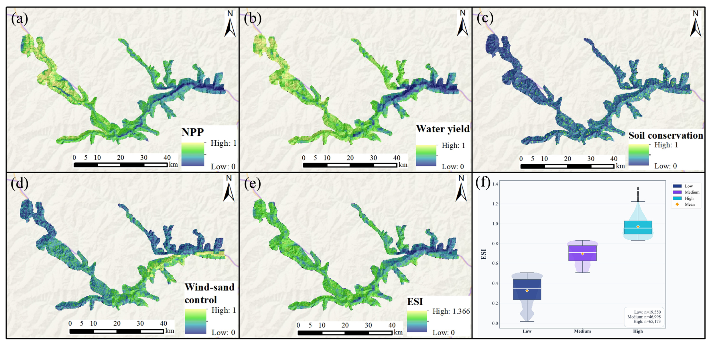
As shown in Figure 4, the ESI of Lixian County is overall at a medium-to-high level, with high-value areas concentrated in mountainous vegetation areas and low-value areas distributed in linear and patchy patterns along valley settlement belts and bare rock areas. The spatial pattern reflects obvious mountain–valley vertical differentiation, closely corresponding to topography and vegetation type distributions. Among the four components, NPP and WY are both high on the vegetated mountain slopes and low in the valley bottoms and on bare rock, whereas SC is more evenly distributed at intermediate values and decreases on the steep, shallow-soiled slopes of the deeply incised valleys. WSC has the lowest mean, and its high values are sparse, being restricted to high-altitude ridges and wind gaps; most of the county is sheltered by terrain and vegetation and has limited demand for windbreak and sand-fixation services. These patterns are directly readable from Figure 4 and are summarised rather than restated.

Figure 4. ESI indicators and results. (a) NPP; (b) Water yield; (c) Soil conservation; (d) Wind-sand control; (e) ESI; (f) ESI at different grades.

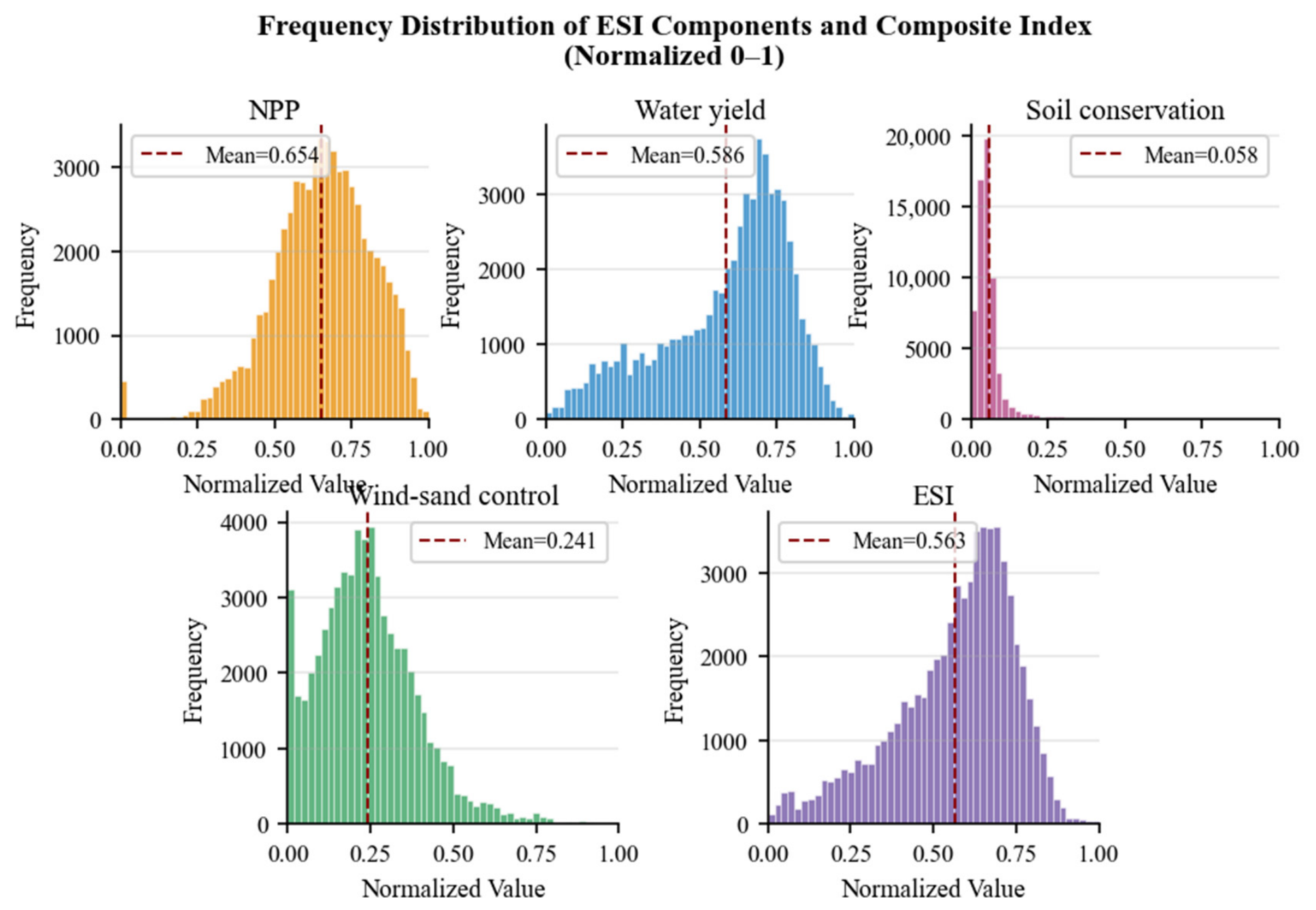
Figure 5 shows the frequency distributions of ESI and its four components after normalisation. The ESI mean is 0.563, and its dispersion is greater than that of RSEI, indicating athat the supply of ecosystem services is more heterogeneous than ecological status itself. NPP has the highest mean (0.654) and the greatest concentration and is the main contributing component; WY (0.587) is approximately normal with slightly thicker tails. SC has a mean of only 0.058 with a strongly right-skewed, L-shaped distribution, and WSC is dominated by low values because wind–sand activity is minimal in Lixian. Two caveats apply to these two components. The low mean of SC is a consequence of its skewed distribution combined with min–max normalisation and should not be read as evidence that soil conservation fails across the county; it indicates that the highest soil-conservation values occur in very few cells, and it should be interpreted together with the absolute values of the SC layer, which average 46,399 (unit to be confirmed). Similarly, the low mean of WSC reflects the weak demand for that service in this area and not a management deficit. Removing WSC from the PCA changed ESI by r = 0.963 (17.7% of the area changed class), which is why it is retained despite its small contribution (Section 2.4).

Figure 5. Frequency distribution of ESI components and composite index.

3.3. GECC Results Analysis

Because the GECC model is calibrated on the locations of historical disasters, it is necessary to state what the resulting index measures. A disaster records a place where the carrying capacity of the geological environment was exceeded, and it provides label data with a clear location and a definite outcome, from which the model learns the association between combinations of factors (for example, lithology and slope) and that outcome [28]. The model output is therefore, strictly, an estimate of geo-hazard susceptibility; GECC is defined as its complement, that is, the modelled probability that the carrying capacity has not been exceeded, so that GECC increases where the terrain has remained stable under the same combination of conditions.

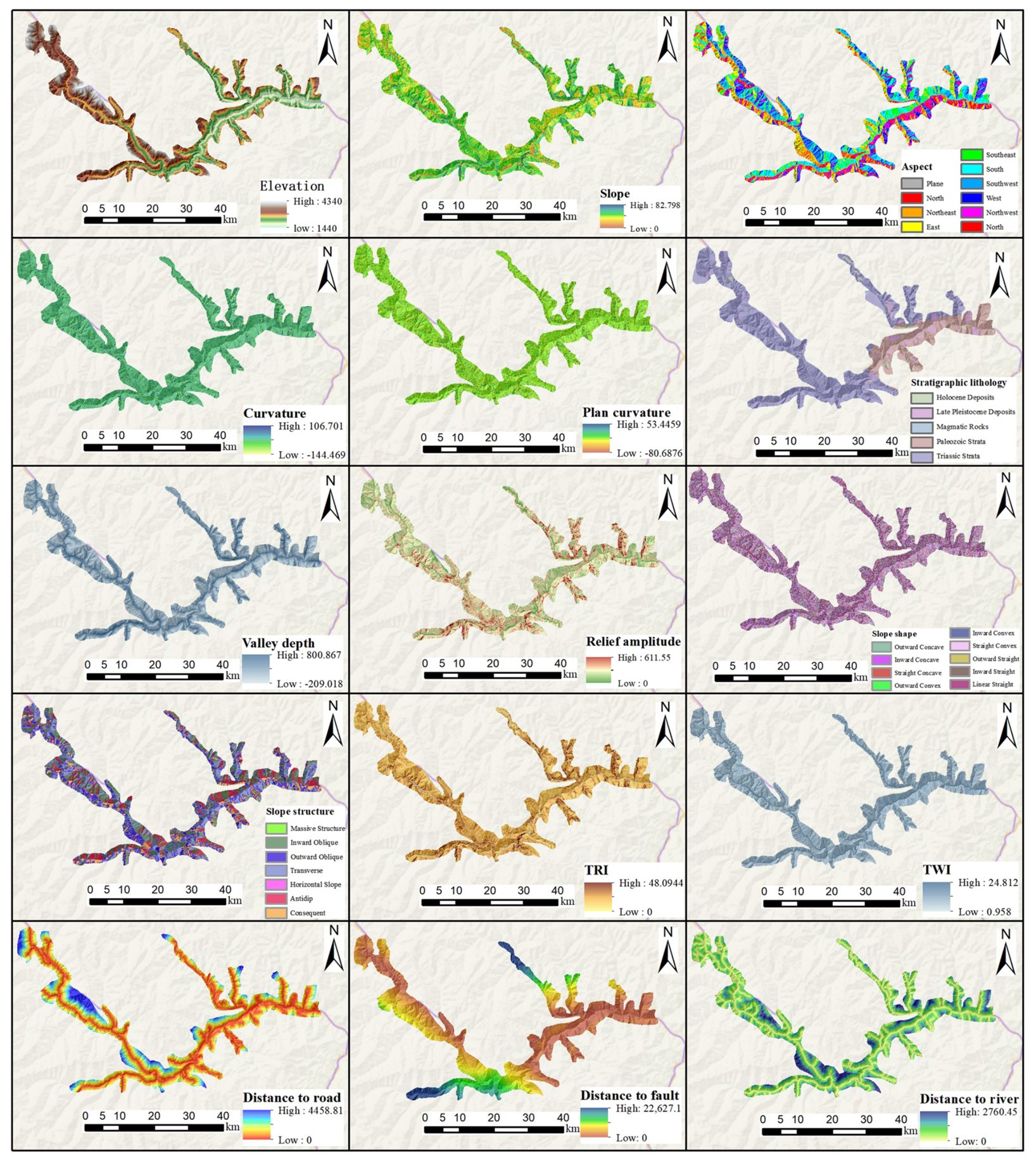
As shown in Figure 6, the 15 factors were selected to represent the three groups that control slope stability in the study area. The terrain group comprises elevation, slope, aspect, curvature (with its profile and plan components), valley depth, relief, slope shape, the Terrain Ruggedness Index and the Topographic Wetness Index: elevation sets the hydrothermal and human activity context [29]; slope governs the balance between driving and resisting forces [30]; aspect redistributes illumination, temperature and precipitation, and thereby weathering and vegetation [31]; the curvature components control the acceleration and convergence of runoff [32]; valley depth expresses the intensity of incision [33]; relief integrates the tectonic and erosional history [34]; slope shape controls the failure mode [35]; TRI indexes surface fragmentation [36]; and TWI indexes moisture accumulation and hence the susceptibility to water-driven failures. The geological group comprises stratum lithology, which determines rock-mass strength [37], and distance to fault, which expresses the influence of tectonic fracturing [38]. The human activity group comprises distance to road, which expresses excavation disturbance [39].

Figure 6. GECC indicators.

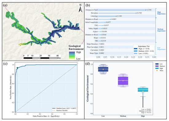
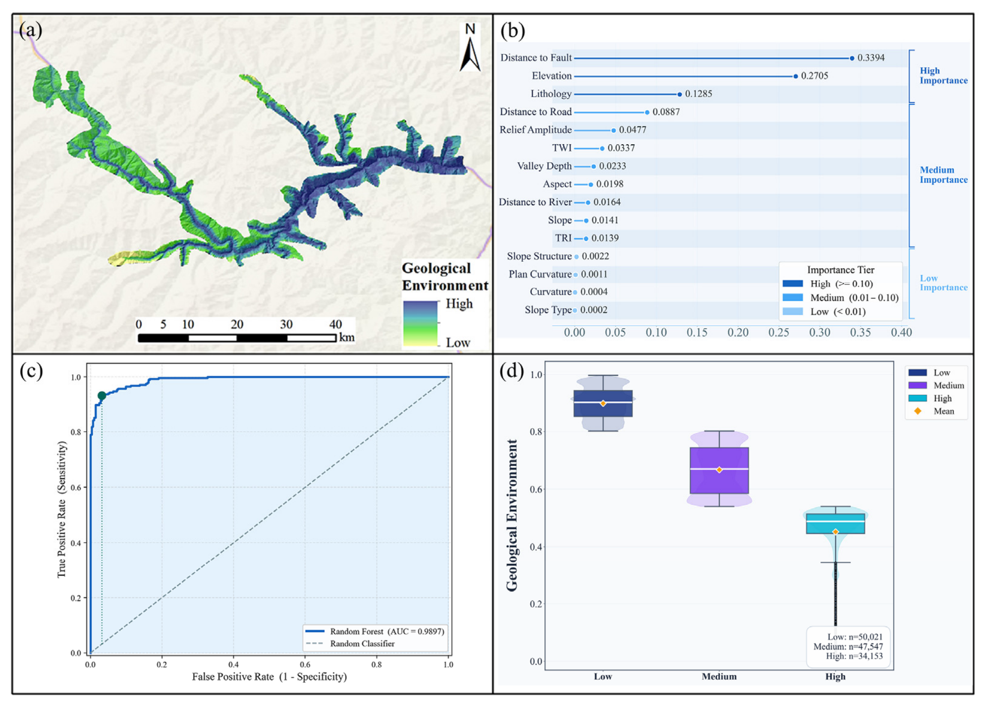
This study employed the RF model, integrating 15 categories of geological environment factors to assess the Geological Environmental Carrying Capacity of the study area. The model was fitted on the 286 historical disaster points and the 284 non-disaster samples. Feature importance analysis results show that distance to fault (33.94%) and elevation (27.05%) are the most important controlling factors, followed by stratum lithology (12.85%) and distance to road (8.87%). This ranking reveals that tectonic activity and elevation differences are the core factors determining the Geological Environmental Carrying Capacity of the study area. The model achieved an AUC of 0.9897 under a random 7:3 split; under spatial block cross-validation, the AUC was 0.981, with a sensitivity of 0.976, a specificity of 0.746 and a precision of 0.795 (confusion matrix in Table 2). A logistic-regression benchmark fitted on the same samples reached AUC = 0.909 under the same random partition and 0.863 under spatial blocking. The lower spatial block value reflects the spatial autocorrelation inherent in the 7:3 random split. The ranking of feature importance was unchanged under both partitions.

Table 2. Predictive performance of the GECC model under two validation schemes and of a simpler benchmark.

Model and Validation Scheme	AUC	Sensitivity	Specificity	Precision	Overall Accuracy
RF, random 7:3 split	0.9897	0.953	0.918	0.921	0.936
RF, 5 km × 5 km spatial block cross-validation (45 blocks, five folds)	0.981	0.976	0.746	0.795	0.861
Logistic regression, same samples	0.909	0.881	0.785	0.805	0.833

Note: the random split is reported for comparability with the earlier literature; the spatial block scheme is the one used to judge the model.

As shown in Figure 7, low-GECC areas form belts along the active fault zones, the deeply incised valleys and the corridors of intensive engineering activity: disaster-point density is elevated within a 2 km buffer of the Minjiang, Huya and Longmenshan back-mountain faults; on the steep (average >35°) slopes of the Minjiang and Dadu river valleys, where bank slopes are scoured by water-level fluctuations; and within 500 m of the G213 and G317 highways, where slopes are cut and loaded. Moderate-GECC areas form a transitional belt on low-to-medium mountains at 2000–3000 m with slopes of 15–35° and alternating soft–hard clastic–carbonate lithology, located 1–3 km from rivers and 3–8 km from major faults; this belt is a grey zone that can degrade to low values under extreme rainfall or seismic triggers. High-GECC areas occupy the gentle denudation planation surfaces of the mid-to-high belts (predominantly 2800–3500 m) and the areas more than 10 km from major faults: slopes are mostly below 15°, human activity is sparse and vegetation cover is high, and more than 85% of the samples fall in the High or Extremely High classes; even above 3800 m, the corresponding share remains about 87–88%.

Figure 7. (a) GECC results, (b) contribution of each indicator, (c) ROC curve, (d) mean values of each GECC level.

3.4. Spatial Coupling Pattern and Vertical Differentiation of RSEI, ESI, and GECC

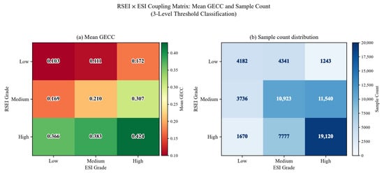
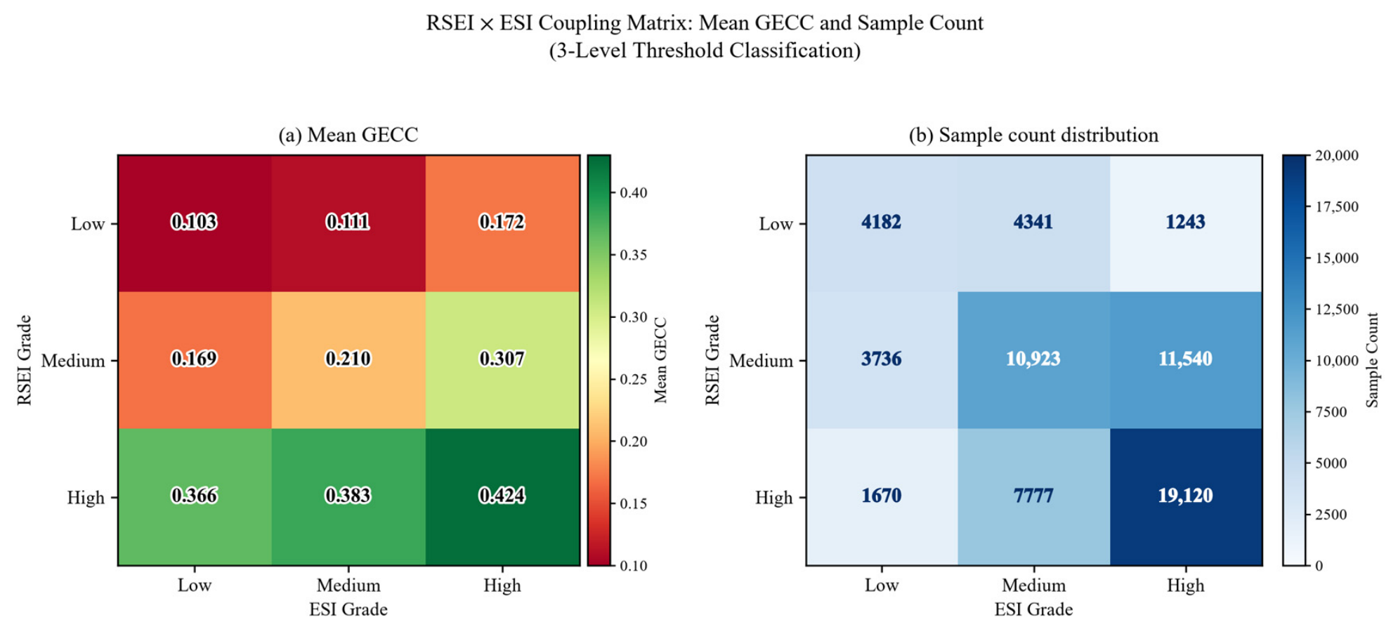
Figure 8 presents the cross-coupling matrix of RSEI and ESI under three-level classification in the study area. Each cell is annotated with the mean GECC and the sample count for the corresponding combination, so that higher values denote higher carrying capacity, intuitively revealing the spatial coupling relationships among the three. From the overall distribution pattern, the study area samples are mainly concentrated along the diagonal: from RSEI Low–ESI Low (4182 samples, 6.5%) to Medium–Medium (10,923, 16.9%) to High–High (19,120, 29.6%), totalling over 53% of all samples. This diagonal clustering phenomenon reflects a moderate positive synergistic relationship between RSEI and ESI [40], indicating that under natural conditions, areas with excellent ecological quality generally also possess strong ecosystem service functions. The two are not independent variables but different characterisation dimensions of the same ecosystem. Notably, the off-diagonal cells RSEI Low–ESI High (only 1243) and RSEI High–ESI Low (only 1670) have significantly lower sample counts, suggesting that structural imbalances of “high ecology but low services” or “low ecology but high services” are not prevalent in the study area.

Figure 8. RSEI × ESI coupling matrix. (a) Mean GECC of each RSEI × ESI combination. (b) Sample count distribution.

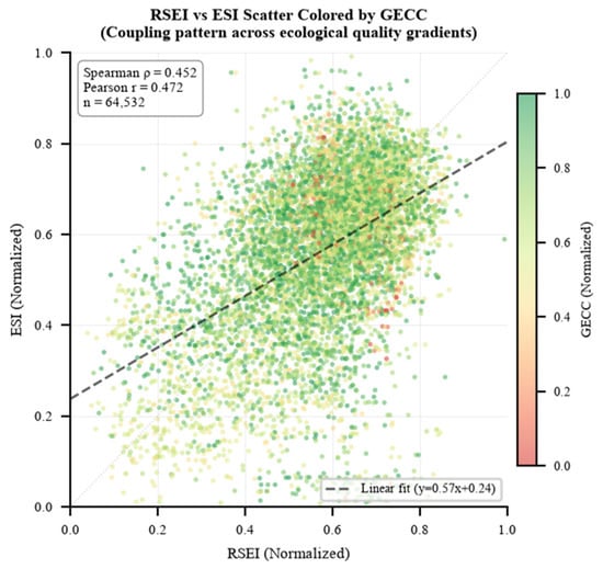
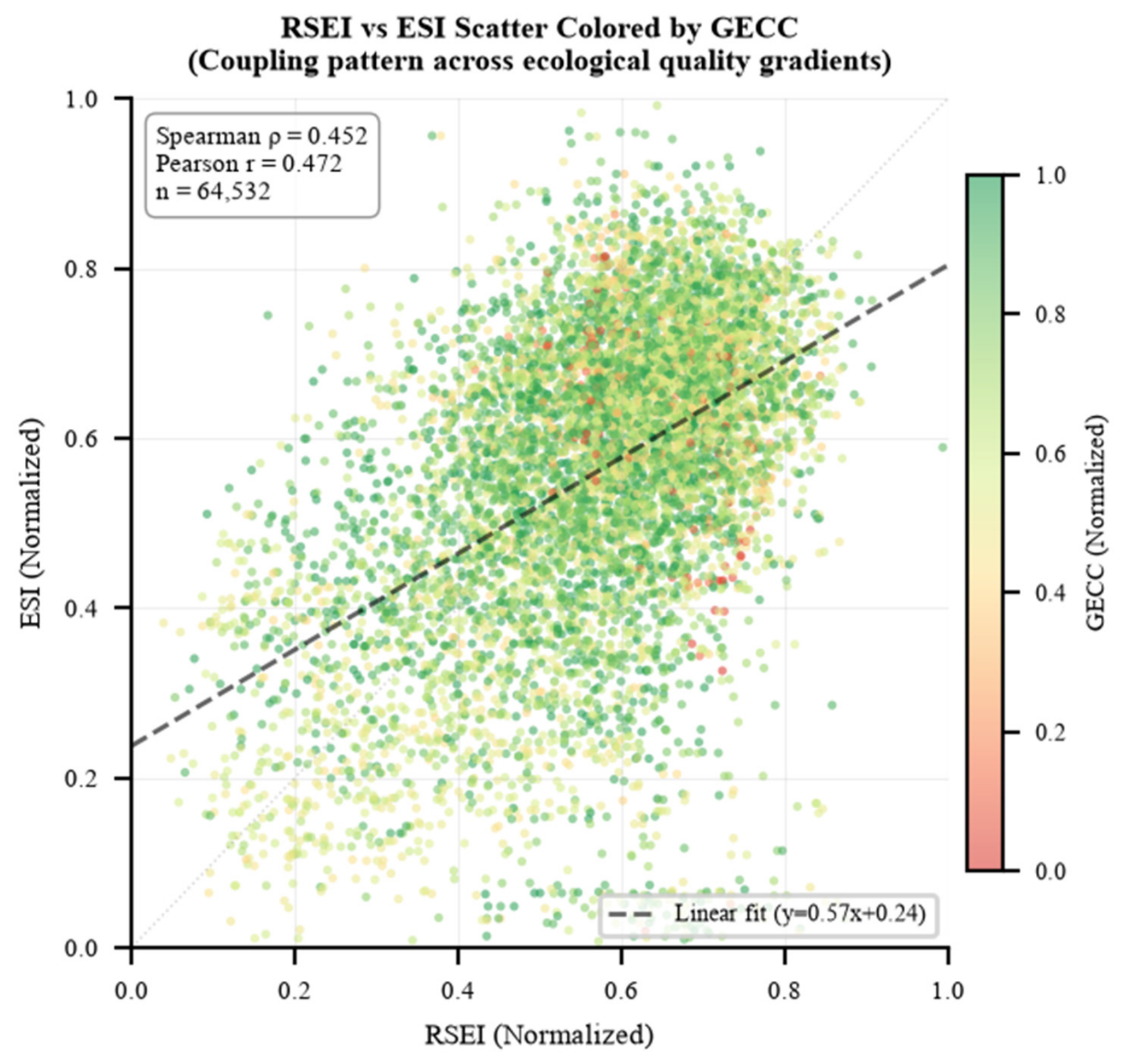
Figure 9 presents the spatial coupling relationship between RSEI and ESI in the form of a scatter plot over the 64,532 grid cells of the study area. On these cells, RSEI and ESI show a moderate positive correlation (Spearman rho = 0.452, n = 64,532) with a positive regression slope, indicating that areas with higher ecological quality generally also have stronger service functions at the macro scale. Because the cells are spatially autocorrelated, the nominal n overstates the number of independent observations, so the correlation is reported as a descriptive statistic of the joint distribution and is not used for significance testing; the effective sample size is only about 3000 independent units at a 1 km block size, about 650 at 2.5 km and about 180 at 5 km. The main body of scatter distribution is concentrated in the rectangular range of RSEI 0.4–0.8 and ESI 0.4–0.8, forming a “dense cloud band” extending along the diagonal, confirming the synchronicity of the two indicators. In the low-value areas where RSEI < 0.3 or ESI < 0.3, scatter density decreases significantly, indicating that extreme low-ecological quality states are rare in the study area. The GECC colour overlay further reveals a pattern that is worth noting: the highest-GECC scatter points are not concentrated in the upper-right corner of the plot (the zone with both high RSEI and high ESI) but are more common in the lower-left to central transitional area. Specifically, GECC rises monotonically with both ecological dimensions across the nine combinations, from 0.103 at RSEI Low × ESI Low (4182 samples) to 0.424 at RSEI High × ESI High (19,120 samples, 29.6%, as shown in Figure 8); the most frequent combination is also the one with the highest mean GECC.

Figure 9. RSEI-ESI scatter plot.

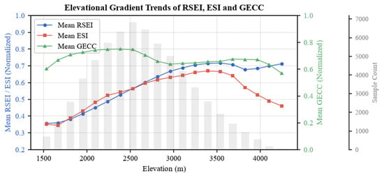
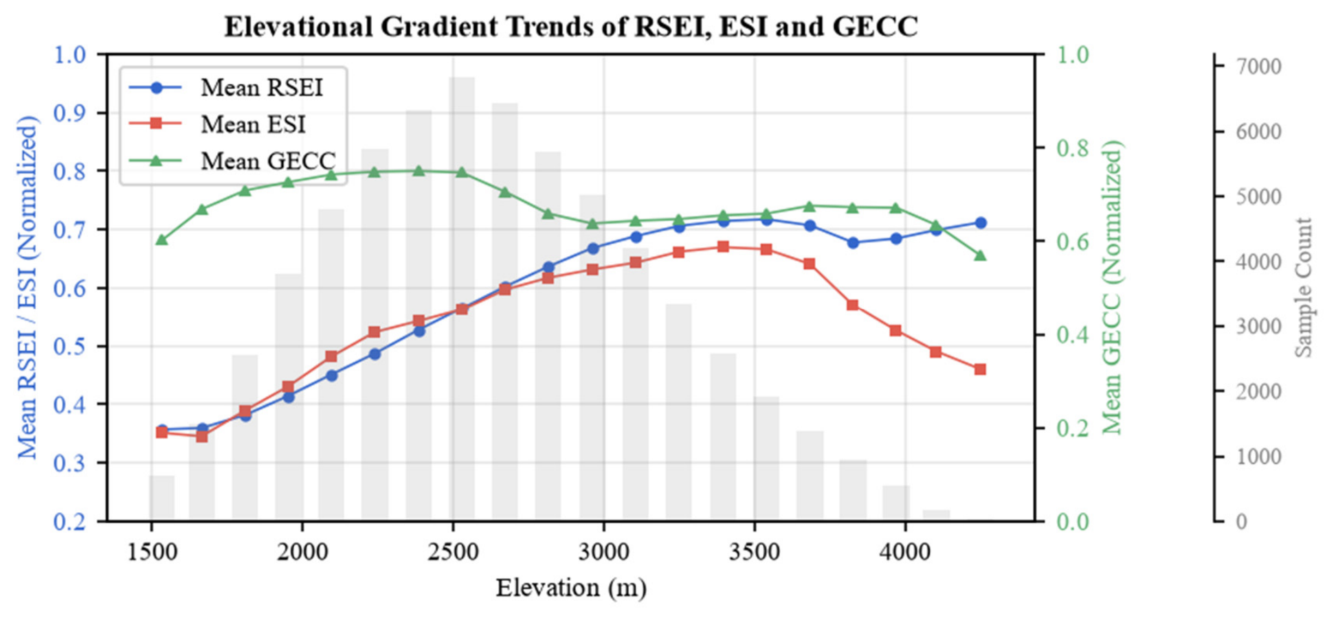
Figure 10 shows the variation trends of RSEI, ESI, and GECC along the altitude gradient. The study area is mainly concentrated in the mid–low elevation belt of 2200–2600 m, with areas above 3800 m accounting for only 2.7%. RSEI increases almost monotonically along the elevation gradient, rising nearly linearly from 0.357 at 1440 m to 0.715 at 3540 m, which is consistent with the combined effect of increasing NDVI and WET and decreasing LST; above 3540 m, it plateaus and fluctuates slightly downward to 0.709, a level we interpret as approaching the altitudinal limit of closed vegetation in the study area, with NDVI returning to low-altitude values. ESI is generally co-directional with RSEI but shows significant differentiation at key stages: the low-altitude starting value (0.492) is higher than RSEI (0.357), benefiting from the service contributions of low-altitude agricultural ecosystems; however, ESI reaches its peak of 0.921 at 3394 m (at an elevation approximately 145 m lower than the RSEI peak), then declines sharply to 0.639 (a 30.6% decrease) in the 3394–4249 m range, due to NPP decreasing from 1277 to 1136 (−11.0%) and water conservation and soil conservation attenuating sharply with vegetation collapse. The GECC trajectory, in contrast, rises with elevation rather than forming an inverted U: it increases from low values at low elevations—where river lateral erosion, fault proximity, and human engineering disturbance dominate—through the mid-elevation belts; reaches and maintains high values across the mid-to-high elevation belts (approximately 2900–3500 m, where the High and Extremely High EGECC classes account for more than 90% of samples); and, while attenuating to a degree above ~3500 m, remains at relatively high levels in the highest belts (above 3800 m, the High and Extremely High classes still account for ~88% of samples). This pattern reflects that low elevations are controlled by river lateral erosion, fault proximity, and human engineering disturbance; mid-elevations (2000–2500 m) have relatively gentle terrain with moderate human disturbance; and high elevations, dominated by gentle denudation planation surfaces, maintain high carrying capacity with only a mild attenuation above ~3500 m from freeze–thaw weathering and steep-slope gravitational potential energy at the uppermost belts. Because this profile is a single-period cross-section, differences between elevation bands may partly reflect other factors that covary with elevation (precipitation, land use and lithology) and should not be attributed to elevation alone.

Figure 10. Variation trends of RSEI, ESI, and GECC along the altitudinal gradient.

3.5. EGECC Results Analysis

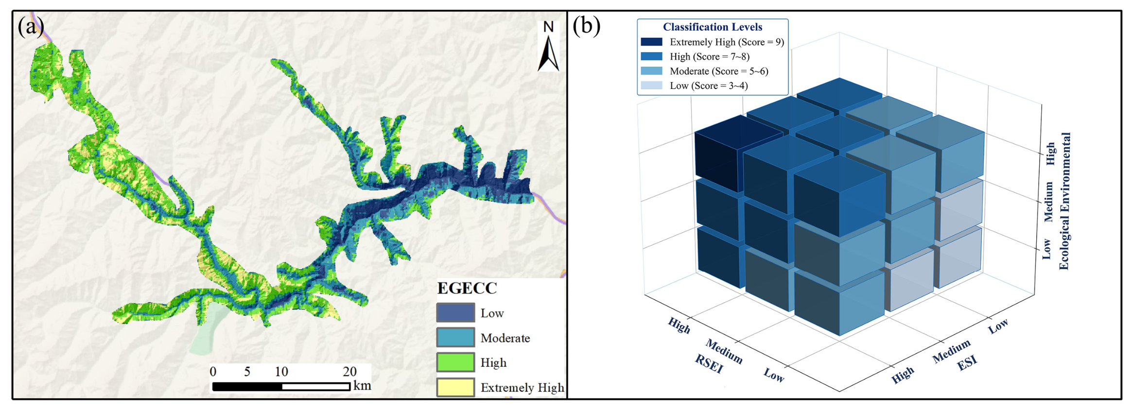
Finally, this study employed a three-dimensional matrix overlay method to spatially couple RSEI, ESI, and GECC, constructing the EGECC and classifying the study area into four comprehensive levels: Low, Moderate, High, and Extremely High (Figure 11); the basic statistics of the three indices in each class are given in Table 3. Among them, the Low level accounts for 16.2% of the study area, with a mean elevation of 2098 m and a mean RSEI of only 0.322 and ESI of 0.347, representing the segment with the lowest ecological indicators among the four levels. It is mainly distributed in low-altitude zones with intensive human activity, where high temperatures, strong drought stress, and infrastructure disturbance from roads and settlements significantly suppress vegetation cover and ecosystem service supply. The Moderate level accounts for 30.4%, with a mean elevation of 2397 m and RSEI (0.528) and ESI (0.510) at intermediate levels, representing a transitional belt (approximately 2200–2500 m) where human activity intensity decreases and natural vegetation recovery begins; it is also the most densely distributed area of the study area. The High level has the largest proportion (39.8%), with a mean elevation of 2853 m, RSEI reaching 0.651 and ESI reaching 0.642, corresponding to mid-to-high altitude tree–shrub mixed forest belts where human activity pressure is significantly reduced, vegetation cover is good, and NPP and water conservation capacity are strong. This is the main bearing area for ecological functions in the study area and the elevation belt with the most concentrated high carrying capacity values. The Extremely High level accounts for 13.7%, with a mean elevation of 3183 m, where RSEI (0.745) and ESI (0.701) both reach their highest class means. However, affected by freeze–thaw weathering and steep-slope gravitational potential energy in high-altitude areas, GECC significantly attenuates above 3500 m, so the Extremely High proportion is limited rather than increasing continuously with elevation.

Figure 11. EGECC results (a) EGECC results; (b) three-dimensional coupling framework.

Table 3. Descriptive statistics of RSEI, ESI and GECC by EGECC class.

EGECC Class	Area Share (%)	Number of Cells	Mean Elevation (m)	RSEI (Mean ± SD)	ESI (Mean ± SD)	GECC (Mean ± SD)
Low	16.2	10,455	2098	0.322 ± 0.111	0.347 ± 0.158	0.090 ± 0.064
Moderate	30.4	19,617	2397	0.528 ± 0.077	0.510 ± 0.168	0.175 ± 0.114
High	39.8	25,684	2853	0.651 ± 0.067	0.642 ± 0.126	0.399 ± 0.151
Extremely High	13.7	8776	3183	0.745 ± 0.063	0.701 ± 0.096	0.529 ± 0.081
Whole study area	100.0	64,532	2637	0.573 ± 0.153	0.563 ± 0.183	0.299 ± 0.194

Note: the ESI values are computed on the final ESI layer used for the classification; the area-weighted mean of each index over the four classes equals its overall mean.

3.6. Sensitivity of the Equal-Weight Aggregation

To test whether the principal findings depend on the equal-weight choice and on the natural-breaks classification, the aggregation was re-run on the 64,532 analysis cells under six alternative weightings of the three ordinal levels—including a doubled weight on each dimension in turn (0.50/0.25/0.25)—and under three alternative classification schemes (quartile and equal-interval thresholds in addition to natural breaks). The cell-level ranking is stable across this range: the weighted kappa against the reported classification is 0.91–1.00 under the alternative weightings and 0.82–0.86 under the alternative schemes, and the ordinal aggregation agrees with a continuous equal-weight integration of the three indices at Spearman ρ = 0.95. Two structural findings hold in every variant: the mean elevation of the four EGECC classes increases monotonically from Low to Extremely High, and the mean GECC increases monotonically across the same order, so the vertical differentiation reported in Section 3.5 does not depend on the equal weights. The area shares of the classes are more sensitive to the classification thresholds than to the weights, and the shares reported in Table 3 are therefore conditional on the natural-breaks classification. Across all these variants, the combined share of the High and Extremely High classes remains within 50.0–62.2%.

4. Discussion

The RSEI-ESI-GECC three-dimensional coupling assessment framework constructed in this study differs methodologically from previous single-dimensional ecological assessment studies. Traditional RSEI focuses on remote sensing spectral signal synthesis and cannot capture the actual supply capacity of ecosystem service functions; ESI has a lagged response to sudden disturbances such as heat waves, droughts, and geological disasters; GECC, Geological Environmental Carrying Capacity, can compensate for the common blind spot of both in predicting the disruptive impact of sudden geological events on ecosystems. The core logic of EGECC lies in the fact that RSEI reflects current ecological status (real-time remote sensing monitoring), ESI reflects the strength of ecological functions (service supply assessment), and GECC reflects whether sudden changes may occur (geological risk early warning). The three mutually verify and complement each other’s blind spots, forming a cognitive chain from status to function to risk. The relationships reported below are spatial associations derived from cross-sectional data.

4.1. Independence and Complementarity of RSEI, ESI, and GECC

Previous RSEI studies have used NDVI as an intuitive representation of ecological quality [41], but in this study RSEI and LST show an almost inverse relationship (Figure 2 and Figure 3): along the altitudinal gradient, LST decreases while RSEI increases, which is consistent with temperature being a constraint on ecological quality in this alpine setting. Because the evidence is cross-sectional, this pattern cannot be separated from the effects of the factors that covary with elevation, such as precipitation, land use and lithology. The coincidence of low-RSEI areas with highway corridors and river erosion belts is likewise consistent with a combined effect of slope cutting and hydrological erosion, and it shows that RSEI responds systematically to surface disturbance intensity in a way that is related to the geological setting.

From the spatial coupling perspective, low-ESI areas coincide with the geologically sensitive areas characterised by large valley depth, steep slopes, proximity to active faults and short distances to highways, which is consistent with valley geomorphology constraining service supply, because the high and steep slopes produced by river downcutting limit vegetation establishment and soil development and thus lower NPP and soil conservation. This is an association, and the cross-sectional data do not allow the individual contributions of slope, lithology and land use to be separated. Furthermore, the four component indicators of ESI reveal differences in the internal mechanisms of ecological function degradation: low-value areas of NPP and WY are mainly concentrated in valleys, reflecting insufficient vegetation productivity and limited water conservation; the extremely low-value areas of SC have the widest range, covering almost all areas with slopes >40°, indicating that topographic conditions are a rigid constraint on soil conservation function; WSC also performs weakly in valley areas, consistent with the arid valley climate characteristics of dry conditions, low precipitation, and bare land surface.

Regarding GECC, Random Forest feature importance analysis shows that distance to fault (33.94%) and elevation (27.05%) have the two highest permutation importances in the fitted model, jointly contributing 61%. Importance ranks the contribution of a factor to the fitted model and should not be read as the magnitude of a causal effect. Although elevation ranks second to distance to fault in feature importance (27.05% vs. 33.94%), it exerts a more pervasive influence on GECC across the full spatial gradient, a distinction that has a clear scale explanation: fault distance is the most direct local determining factor when assessing carrying capacity strength point by point; while elevation, as a comprehensive proxy indicator for temperature, slope, and stratum stability, has stronger co-variation with GECC on the full-domain spatial gradient.

The RSEI (0.688) and ESI (0.912) of GECC High areas are significantly higher than those of GECC Low areas (RSEI = 0.465, ESI = 0.644), because high-GECC areas in the study area are mostly located in the mid-to-high-altitude belts with gentle terrain and well-preserved vegetation, where ecological conditions are also favourable; while the low-GECC areas, concentrated in fault zones, deeply incised valleys, and intensively used low-altitude belts, generally show depressed ecological indicators. Nevertheless, a minority of low-GECC samples fall in transitional zones with acceptable (though not high) ecological indicators, and these are precisely the areas where ecology-only assessment would fail: regional ecological stability cannot be judged solely by high RSEI or ESI values, because moderate ecological status may overlay weak geological carrying capacity. Incorporating GECC into the comprehensive assessment framework is precisely what reveals this identification blind spot.

4.2. Coupling–Decoupling Mechanism and Altitudinal Vertical Differentiation

Approximately one-third of the samples exhibit significant deviation between RSEI and ESI. The RSEI-leading type is concentrated in high-altitude, low-temperature areas: high RSEI essentially stems passively from low ground temperature rather than actively superior ecological quality, but substantive service functions such as NPP and WY are doubly constrained by short growing seasons and shallow soil layers; the ESI-leading type is concentrated in mid-altitude optimal hydrothermal zones: service functions are fully expressed, but RSEI is suppressed by relatively high temperatures. A single-RSEI assessment ranks the former too high and the latter too low relative to the two-index view, while the dual-indicator framework identifies such blind spots systematically.

This paper selects altitude rather than combinations of terrain factors as the analytical axis. The reason is that distance to fault is a point-source variable whose information is concentrated in the narrow buffer zones on both sides of the faults and which loses discriminative power at greater distances, whereas altitude is a continuous, domain-wide variable that co-varies simultaneously with temperature, precipitation, vegetation zones, slope and lithology, and thus provides a single scale along which all three indices can be profiled [42]. Along this axis, RSEI rises almost monotonically and saturates at mid-to-high elevations, while ESI continues to rise and peaks at about 3394 m; this peak separation implies that an assessment based on RSEI alone would rank the mid-to-high transitional belts lower than one that also considers services. The eco-geological pattern is equally systematic: in the 2500–3500 m band, RSEI and ESI are high while the High and Extremely High EGECC classes dominate, whereas the fault-dense, low-altitude valleys combine lower ecological indicators with low GECC. We read this as spatially structured co-variation rather than as evidence of a specific mechanism: because the analysis is a single-period cross-section, the between-band differences may partly reflect factors other than elevation, and the direction of any causal link cannot be established from these data. What the three-dimensional framework does add is the identification of the coupled low-ecology–low-capacity zones that a single- or dual-indicator system cannot separate, even though it cannot by itself establish why they are coupled.

4.3. Mechanism and Spatial Pattern of EGECC Comprehensive Assessment

EGECC classifies the study area into four comprehensive levels: Low (16.2%), Moderate (30.4%), High (39.8%), and Extremely High (13.7%). Each level shows clear progressive differentiation along altitude: the Low level has a mean elevation of 2098 m, concentrated in low-altitude valley areas with dense human activity; the Moderate level corresponds to a transitional belt of decreasing human activity and beginning natural vegetation recovery; the High level has the largest proportion (39.8%), corresponding to mid-to-high altitude tree–shrub mixed forest belts, serving as the main bearing area for ecological functions in the study area; the Extremely High level has a mean elevation of 3183 m but accounts for only 13.7%, constrained by high-altitude GECC attenuation and not expanding continuously with elevation. EGECC levels are primarily associated with GECC: from Low to Extremely High, the mean GECC increases by a factor of 5.88, compared with factors of 2.11 for RSEI and 2.25 for ESI (Table 3). Because the three indices were entered with equal weights and were classified separately before the overlay, this difference shows that the geological dimension varies over a wider range of the classified scale in this study area; it does not by itself establish that geological conditions are causally more important, and it is partly a consequence of the equal-weight and natural-breaks choices (Section 2.6). What this does establish is that the geological dimension is not reproducible as a linear combination of the two ecological dimensions and that it therefore constitutes a third information dimension that is independent of ecological physical status and service functions. Omitting the geological dimension is therefore not a neutral simplification: when the framework is reduced to RSEI + ESI and the two-dimensional composite is reclassified with the same four-level scheme, cells that the three-dimensional scheme places in the Low or Moderate classes are classified as safe. These cells are not a marginal remainder: they number 17,684, i.e., 27.4% of all cells and 59.1% of the Low and Moderate classes, and their mean GECC is 0.159, close to half the regional mean, whereas their mean RSEI (0.532) and ESI (0.541) are close to the regional values (0.573 and 0.562). They are therefore not separable from the remainder of the study area by either ecological dimension, and the risk they carry is visible only through the geological dimension. Relative to the other Low and Moderate cells, they lie at a higher elevation (2319 m against 2123 m) and farther from the mapped faults (3413 m against 1893 m), so this exposure would not be detected by restricting attention to fault zones or to the low-altitude valleys.

4.4. Policy Implications and Management Recommendations

Building on the above three-dimensional framework analysis, this study proposes a five-tier hierarchical management strategy. The first tier is spatial zoning control, with the integrated EGECC grade as the primary basis for regionalisation: the extremely high-grade zone is designated as an ecological conservation redline core area with strict restrictions on development and construction; the high-grade zone maintains the status quo and moderately develops eco-tourism and a sustainable understory economy; the medium-grade zone implements targeted remediation, addressing its specific shortcomings (GECC-constrained units prioritise geological hazard control, RSEI-constrained units prioritise vegetation restoration, and ESI-constrained units prioritise service-function enhancement); and the low-grade zone treats reducing the intensity of human activities as the primary measure. The second tier is coupling–decoupling early warning: a remote-sensing–service decoupling warning line is established for RSEI High/ESI Medium coupling-conflict units; RSEI-advanced and ESI-advanced areas are designated as early-warning zones for latent degradation, with intensified monitoring.

The third tier is targeted ecological function maintenance: because WET is more strongly related to RSEI than NDVI is (Pearson r = 0.696 vs. 0.596, n = 64,532), measures that maintain surface moisture should be prioritised; and because the spatial patterns of SC and WSC differ from those of NPP and WY, service-oriented management should be differentiated by the locally dominant service rather than applied uniformly. The fourth tier is the coordinated governance of geological hazards and ecology, replacing traditional rigid structures with near-natural methods in the fault-dense, low-altitude valleys and settlement belts where ecological degradation and geological risk co-occur and establishing a geo-ecological joint monitoring network. The fifth tier is dynamic adaptive management, with reassessments conducted every 3–5 years.

Within this strategy, the comparison between the two- and three-dimensional schemes has a direct planning implication: because the two-dimensional RSEI + ESI scheme can classify areas as safe that the three-dimensional scheme places in a lower class, ecological indicators alone should not be used to approve construction sites. Geological conditions must therefore be treated as a precondition for residential-site layout and building construction, and a four-dimensional collaborative framework—ecological status, service function, geological safety and human-settlement adaptation—should be adopted for planning evaluation.

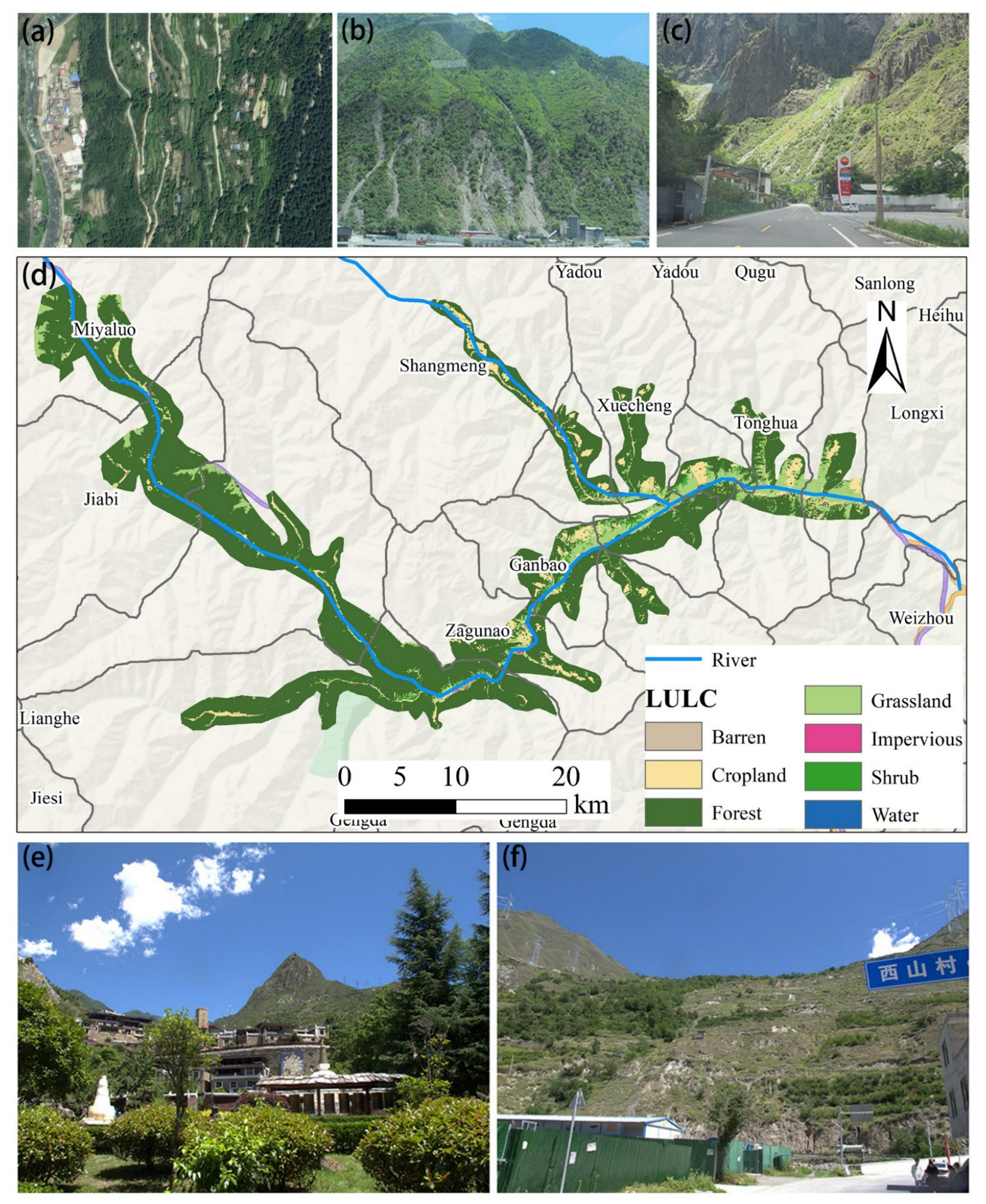
Within the county, elements at risk are highly concentrated in the Zagunao River valley: the Tibetan and Qiang ethnic groups account for 86.9% of the population, settlements are scattered in a ribbon pattern along the river and its tributaries, and numerous villages sit on ancient landslide, collapse, and debris-flow deposits as well as river floodplains; most houses are Tibetan-style stone–wood structures with masonry composed of weak rocks such as the phyllite, slate, and schist of the Weiguanguan and Zagunao formations. On this basis, valley deposits and floodplains should be treated as areas where new construction requires a site-specific geotechnical assessment. It should be stressed that EGECC is a regional screening tool and cannot replace such an assessment or a location-specific risk analysis, so the recommendation is to require the assessment before approval rather than to prescribe particular engineering solutions, which lie outside what the present data can support.

The riverside G317 National Highway, the Wema Expressway and the low-grade rural roads should be integrated into the geological hazard early-warning and emergency traffic-preservation system; as shown in Figure 12, elements at risk are concentrated along the Zagunao River valley in a ribbon pattern, with numerous villages situated on ancient landslide, collapse and debris-flow deposits and floodplains, which corroborates the spatial pattern identified above.

Figure 12. LULC map and field photographs of Lixian County: (a) Xiameng Township landslide, (b) geological hazard occurrence area, (c) roadside geological hazard occurrence area, (d) spatial distribution of LULC in Lixian County, (e) traditional Tibetan–Qiang stone–wood village settlement, (f) Xishan Village and its surrounding geo-hazard environment.

Areas placed in the Low or Moderate EGECC classes, and the slopes and fault-proximate zones within them, are the priority targets for restricting new construction, for protecting and reinforcing existing stone–wood dwellings, and for near-natural slope stabilisation. Recommendations on specific land uses—for example, the siting of fruit–forest bases in the warm low-elevation valleys or the maintenance of native meadow grazing in the high-cold zones—are presented as options consistent with the assessed eco-geological gradient, and each would require site-level verification before implementation. In the high-carrying-capacity gentle river-valley areas, which are the main distribution zones of towns and concentrated villages, settlement layout should be optimised and renovation criteria for stone–wood dwellings standardised, while hazard-prone belts should be strictly avoided.

Vertically, the 2500–3500 m belt combines the most favourable ecological conditions with high modelled carrying capacity in this study, so the management implication is the opposite of the wording used in the earlier version of this manuscript: this belt is not geologically weak, but its carrying capacity depends on the maintenance of vegetation cover, so new construction and building volume should be controlled and slope cutting avoided. Valleys below 2500 m, where ESI exceeds RSEI, should coordinate settlement improvement with ecological conservation, and areas above 3500 m, where RSEI exceeds ESI, should strictly control new construction and disturbance. In the medium-carrying-capacity mid-mountain slopes, traditional Tibetan–Qiang villages should follow protective development with strict control of new construction; in the mountain slopes and fault-proximity zones classified as Low or Extremely High EGECC, consolidation should be implemented and new human-settlement development avoided.

In summary, the coupling pattern revealed by the assessment can guide the construction of a full-chain system of “zoning control–risk early warning–building upgrading–coordinated governance–dynamic regulation”: priority should be given to avoiding fault zones and steep slopes, and ecological restoration, slope treatment and soil–water conservation works should be targeted according to coupling characteristics; an eco–geo–habitat decoupling early-warning mechanism should be incorporated into dynamic monitoring. The three-dimensional coupled assessment thus supports a shift in the planning of Lixian from single-dimensional ecological control and passive geological prevention toward proactive, territorially adapted collaboration among ecology, service, geology and habitat, and provides a reference basis for the human-settlement planning and eco-geological coordinated governance of ecologically fragile counties in the high-mountain canyon regions of northwestern Sichuan.

4.5. Limitations and Prospects

This comprehensive analysis based on multi-source ecological and geological information has revealed the spatial coupling patterns and key contradictions of the eco-geological system in the study area and provides a baseline reference for ecological security assessment and management decision-making in alpine gorge areas. The scope of the results is bounded by the following conditions. (1) Temporal: The analysis is based on single-period cross-sectional data, so the RSEI–ESI decoupling relationship and the GECC threshold effects describe the state of the study area at that period; part of the differentiation between elevation bands may reflect between-site rather than elevation-controlled differences, and a multi-year series is needed to establish their temporal stability. (2) Data consistency: The Landsat 8 scenes, the DEM and the historical disaster inventory are not strictly contemporaneous (Section 2.2); because lithology, fault structure and terrain change slowly, this is unlikely to alter the main pattern, but it does add to the uncertainty. (3) Weighting and classification: The three dimensions were combined with equal weights and the levels were defined by natural breaks (Jenks). Both choices follow standard practice in comparable three-dimensional assessments. (4) Model validation: The AUC of the RF model is 0.990 under a random 7:3 split and 0.981 under spatial block cross-validation; the difference reflects the spatial autocorrelation among the training samples. Validation against independent spatio-temporal samples would further constrain the performance estimate. (5) Definition of GECC: GECC is derived from a geo-hazard susceptibility model and therefore carries the completeness and positional accuracy of the disaster inventory; it quantifies the modelled absence of past failure. (6) Scale and transferability: The framework was tested in a single county, and applying it to other alpine gorge settings requires site-specific parameterisation and verification of the management recommendations in Section 4.4. (7) Analyses not carried out: No confidence interval was computed for the AUC; no independent external validation dataset (for example, a disaster inventory from a neighbouring county, or deformation points identified by InSAR) was available to the study, so the spatial block cross-validation remains the strongest way of checking model performance; and no uncertainty or confidence map of EGECC was produced. The sensitivity of the equal-weight aggregation to six alternative weightings of the three ordinal levels and to three alternative classification schemes and the comparison of the ordinal aggregation with a continuous equal-weight integration are reported in Section 3.6. These four items are stated here as limitations rather than reported as results, and they define the margin of uncertainty within which the EGECC pattern should be read. Future research can be extended in the following directions: introducing Landsat/Sentinel multi-temporal data to verify the temporal stability of the model and the influence of seasonal phenology and embedding the three-dimensional framework into spatial planning decision support systems, so that managers can simulate the impact of different conservation scenarios on EGECC levels on an interactive platform and move from static assessment to scenario simulation.

5. Conclusions

This study takes Lixian County, Sichuan Province, as a typical alpine gorge area and constructs an EGECC three-dimensional coupling framework integrating RSEI, ESI and GECC and uses it to describe the spatial coupling and vertical differentiation of ecological quality, service functions and geological conditions. Three results are highlighted. First, RSEI and ESI are only moderately correlated, and their altitudinal peaks are separated, indicating that surface physical status and ecological processes should be assessed separately. Second, GECC varies over a wider range of the composite scale than the two ecological dimensions and is not reproducible from them; consequently, removing it from the framework reclassifies a proportion of the area as safe that the three-dimensional framework places in a lower class. Third, the coupling is organised systematically according to altitude: the 2500–3500 m belt combines favourable ecological conditions with high modelled carrying capacity, whereas the fault-dense, low-altitude valleys combine lower ecological indicators with low carrying capacity. A five-tier management strategy is outlined on this basis. The contribution of the framework is that it makes the three dimensions comparable on a common grid and shows what is lost when one of them is dropped; it is a tool for regional eco-geological zoning. Because the analysis rests on single-period cross-sectional data from one county, further verification with multi-temporal data and additional study areas is needed before the framework can be applied to other alpine gorge regions.

References

- Ellili, N.O.D. Bibliometric analysis of sustainability papers: Evidence from Environment, Development and sustainability. Environ. Dev. Sustain. 2024, 26, 9923–9944. [Google Scholar] [CrossRef] [Scilit]
- Huang, J.; Zhang, Y.; Zhang, J.; Qi, J.; Liu, P.; Liang, C. Eco-Geological Environment Quality Assessment Based on FAHP-CV Combination Weighting. Sustainability 2023, 15, 18. [Google Scholar] [CrossRef] [Scilit]
- Qi, J.; Zhang, Y.; Zhang, J.; Chen, Y.; Wu, C.; Duan, C.; Cheng, Z.; Pan, Z. Research on the Evaluation of Geological Environment Carrying Capacity Based on the AHP-CRITIC Empowerment Method. Land 2022, 11, 17. [Google Scholar] [CrossRef] [Scilit]
- Jiang, L.; Liu, Y.; Wu, S.; Yang, C. Analyzing ecological environment change and associated driving factors in China based on NDVI time series data. Ecol. Indic. 2021, 129, 9. [Google Scholar] [CrossRef] [Scilit]
- Qi, T.; Meng, X.; Chang, J.; Yue, D.; Wang, Y.; Chen, G. Landslide utilization and driving mechanisms in alpine gorge areas of the eastern Qinghai-Tibet Plateau. Catena 2025, 249, 14. [Google Scholar] [CrossRef] [Scilit]
- Zhang, X.; Xu, X.; Li, X.; Cui, P.; Zheng, D. A new scheme of climate-vegetation regionalization in the Hengduan Mountains Region. Sci. China Earth Sci. 2024, 67, 751–768. [Google Scholar] [CrossRef] [Scilit]
- Sun, C.; Li, J.; Liu, Y.; Cao, L.; Zheng, J.; Yang, Z.; Ye, J.; Li, Y. Ecological quality assessment and monitoring using a time-series remote Sensing Ecological Index (ts-RSEI). GISci Remote Sens. 2022, 59, 1793–1816. [Google Scholar] [CrossRef] [Scilit]
- Li, Y.; Wu, L.; Han, Q.; Wang, X.; Zou, T.; Fan, C. Estimation of remote sensing based ecological index along the Grand Canal based on PCA-AHP-TOPSIS methodology. Ecol. Indic. 2021, 122, 13. [Google Scholar] [CrossRef] [Scilit]
- Guo, Y.; Zhan, M.; Xu, H.; Li, X.; Fang, J.; Zhou, X.; Lin, D.; Chen, W. MRSEILA: A modified remote sensing ecological index using local adaptability for enhancing ecological environment quality assessment. Ecol. Inf. 2025, 90, 15. [Google Scholar] [CrossRef] [Scilit]
- Liu, Y.; Liu, H.; Xu, W.; Wang, L.; Kou, W.; Lu, N.; Ou, G. Comparing the applicability between Landsat and MODIS datasets for eco-environment quality assessment: A case study of the Yunnan-Guizhou Plateau, China. Geo-Spat. Inf. Sci. 2025, 29, 24. [Google Scholar] [CrossRef] [Scilit]
- Kou, L.; Wang, X.; Wang, H.; Wang, X.; Hou, Y. Spatiotemporal analysis of ecological benefits coupling remote sensing ecological index and ecosystem services index. Ecol. Indic. 2024, 166, 14. [Google Scholar] [CrossRef] [Scilit]
- Tang, X.; Liu, Y.; Pan, Y. An Evaluation and Region Division Method for Ecosystem Service Supply and Demand Based on Land Use and POI Data. Sustainability 2020, 12, 14. [Google Scholar] [CrossRef] [Scilit]
- Ma, Y.; Feng, Y.; Ke, J.; Zhang, C. Spatial and temporal characteristics of vegetation carbon sequestration in Beijing and regional division strategies. Environ. Dev. Sustain. 2025. [Google Scholar] [CrossRef] [Scilit]
- Zhang, J.; Chen, S. Evaluating water conservation capacity in the Yellow River water conservation area integrating ecological model and machine learning. J. Hydrol. 2025, 663, 16. [Google Scholar] [CrossRef] [Scilit]
- Li, Y.; Chen, J.; Zhou, F.; Bao, Y.; Li, Z.; Wang, Q. Deformation characteristics and reactivated failure modes of the massive Baimu ancient landslide deposit on the northern margin of the East Himalayan syntaxis. Earth Surf. Process. Landf. 2024, 49, 1667–1681. [Google Scholar] [CrossRef] [Scilit]
- Li, X. TOPSIS model with entropy weight for eco geological environmental carrying capacity assessment. Microprocess. Microsyst. 2021, 82, 8. [Google Scholar] [CrossRef] [Scilit]
- Guo, Y.; Huang, Y.; Li, J.; Ouyang, S.; Wang, J.; Wu, L. Study on the evolution law of fractional vegetation cover in mining areas with different eco-geological environmental carrying capacities and its driving factors. Environ. Dev. Sustain. 2025. [Google Scholar] [CrossRef] [Scilit]
- Ali, M.Z.; Chen, K.J.; Shafique, M.; Adnan, M.; Zheng, Z.; Zhang, W.; Qing, Z. High-resolution landslide mapping and susceptibility assessment: Landslide temporal variations and vegetation recovery. Adv. Space Res. 2024, 74, 3668–3690. [Google Scholar] [CrossRef] [Scilit]
- Rengers, F.K.; Mcguire, L.A.; Oakley, N.S.; Kean, J.W.; Staley, D.M.; Tang, H. Landslides after wildfire: Initiation, magnitude, and mobility. Landslides 2020, 17, 2631–2641. [Google Scholar] [CrossRef] [Scilit]
- Zhao, N.; Du, L.; Tian, S.; Zhang, B.; Zheng, X.; Li, Y. Cropland Expansion Masks Ecological Degradation: The Unsustainable Greening of China’s Drylands. Agronomy 2025, 15, 23. [Google Scholar] [CrossRef] [Scilit]
- Zhang, M.; Kafy, A.-A.; Ren, B.; Zhang, Y.; Tan, S.; Li, J. Application of the Optimal Parameter Geographic Detector Model in the Identification of Influencing Factors of Ecological Quality in Guangzhou, China. Land 2022, 11, 20. [Google Scholar] [CrossRef] [Scilit]
- Aydin, N.Y.; Balcik, F.B. Assessing long-term eco-environmental quality dynamics in Akarçay River Basin (1985–2020) using Remote Sensing Ecological Index (RSEI). Environ. Earth Sci. 2025, 84, 24. [Google Scholar] [CrossRef] [Scilit]
- Zhang, J.; Jiao, G.; Ye, Q.; Gu, X. The Impact of Urban Expansion on the Urban Thermal Environment: A Case Study in Nanchang, Jiangxi, China. Sustainability 2022, 14, 22. [Google Scholar] [CrossRef] [Scilit]
- Liu, J.; Liu, G.; Ma, Z.; Chen, F.; Wu, Y.; Ge, C.; Wang, X. Evaluation of Geoenvironment Carrying Capacity in Mineral Resource-Based Cities from the Perspective of Sustainable Development. Sustainability 2024, 16, 14. [Google Scholar] [CrossRef] [Scilit]
- Wang, Y.; Yuan, M.; Zhou, X.; Qu, X. Evaluation of Geo-Environment Carrying Capacity Based on Intuitionistic Fuzzy TOPSIS Method: A Case Study of China. Sustainability 2023, 15, 21. [Google Scholar] [CrossRef] [Scilit]
- Zhang, M.; Tan, S. Multi-Source Weighting Integration for Evaluating the Eco-Geological Environmental Carrying Capacity in Kunming, China. Land 2026, 15, 28. [Google Scholar] [CrossRef] [Scilit]
- Breiman, L. Random forests. Mach. Learn. 2001, 45, 5–32. [Google Scholar] [CrossRef] [Scilit]
- Ni, D.; Gong, C.; Ding, D.; Tian, Y. Geological environment carrying capacity assessment using remote sensing and integrated modeling: A case study of Yi’an district, Tongling, China. Adv. Space Res. 2025, 75, 6274–6286. [Google Scholar] [CrossRef] [Scilit]
- Zhao, J.; Zhang, Q.; Wang, D.; Wu, W.; Yuan, R. Machine Learning-Based Evaluation of Susceptibility to Geological Hazards in the Hengduan Mountains Region, China. Int. J. Disaster Risk Sci. 2022, 13, 305–316. [Google Scholar] [CrossRef] [Scilit]
- Su, Y.; Li, R.; Li, M. Susceptibility Assessment and Deformation Prediction of Highway Slope Geological Hazards Based On Game Theory and ICEEMDAN-WTC-Itransformer. PFG-J. Photogramm. Remote Sens. Geoinf. Sci. 2026, 94, 21. [Google Scholar] [CrossRef] [Scilit]
- He, Z.; Yu, M.; Li, J. Evaluation of geological hazard susceptibility in loess disaster area based on gis technology. Fresenius Environ. Bull. 2022, 31, 10708–10715. [Google Scholar]
- Bi, X.; Fan, Q.; He, L.; Zhang, C.; Diao, Y.; Han, Y. Analysis and Evaluation of Extreme Rainfall Trends and Geological Hazards Risk in the Lower Jinshajiang River. Appl. Sci. 2023, 13, 18. [Google Scholar] [CrossRef] [Scilit]
- Andriani, G.F.; Loiotine, L. Multidisciplinary approach for assessment of the factors affecting geohazard in karst valley: The case study of Gravina di Petruscio (Apulia, South Italy). Environ. Earth Sci. 2020, 79, 16. [Google Scholar] [CrossRef] [Scilit]
- Ma, S.; Shao, X.; Xu, C. Delineating Non-Susceptible Landslide Areas in China Based on Topographic Index and Quantile Non-Linear Model. Forests 2024, 15, 16. [Google Scholar] [CrossRef] [Scilit]
- Yang, W.; Niu, R.; Si, R.; Li, J. Geological Hazard Susceptibility Analysis and Developmental Characteristics Based on Slope Unit, Using the Xinxian County, Henan Province as an Example. Sensors 2024, 24, 19. [Google Scholar] [CrossRef] [Scilit]
- Grabowski, D.; Laskowicz, I.; Malka, A.; Rubinkiewicz, J. Geoenvironmental conditioning of landsliding in river valleys of lowland regions and its significance in landslide susceptibility assessment: A case study in the Lower Vistula Valley, Northern Poland. Geomorphology 2022, 419, 24. [Google Scholar] [CrossRef] [Scilit]
- Ahmed, I.; Shang, Y.; Wang, X.; Hassan, M. Spatial heterogeneity of rock mass degradation and landslide susceptibility in the fault damage zone, Northwestern Himalayas, Pakistan. Bull. Eng. Geol. Environ. 2026, 85, 24. [Google Scholar] [CrossRef] [Scilit]
- Yu, B.; Li, H.; Xing, H.; Ge, W.; Zhou, L.; Zhang, J.; Xu, M.; Yu, C. Geospatial SHAP interpretability for urban road collapse susceptibility assessment: A case study in Hangzhou, China. Geomat. Nat. Hazards Risk 2025, 16, 23. [Google Scholar] [CrossRef] [Scilit]
- Li, M.; Li, L.; Lai, Y.; He, L.; He, Z.; Wang, Z. Geological Hazard Susceptibility Analysis Based on RF, SVM, and NB Models, Using the Puge Section of the Zemu River Valley as an Example. Sustainability 2023, 15, 21. [Google Scholar] [CrossRef] [Scilit]
- Bennett, E.M.; Peterson, G.D.; Gordon, L.J. Understanding relationships among multiple ecosystem services. Ecol. Lett. 2009, 12, 1394–1404. [Google Scholar] [CrossRef] [Scilit]
- Hu, X.; Xu, H. A new remote sensing index for assessing the spatial heterogeneity in urban ecological quality: A case from Fuzhou City, China. Ecol. Indic. 2018, 89, 11–21. [Google Scholar] [CrossRef] [Scilit]
- Wu, J.; Wang, G.; Chen, W.; Pan, S.; Zeng, J. Terrain gradient variations in the ecosystem services value of the Qinghai-Tibet Plateau, China. Glob. Ecol. Conserv. 2022, 34, 15. [Google Scholar] [CrossRef] [Scilit]
Disclaimer/Publisher’s Note: The statements, opinions and data contained in all publications are solely those of the individual author(s) and contributor(s) and not of MDPI and/or the editor(s). MDPI and/or the editor(s) disclaim responsibility for any injury to people or property resulting from any ideas, methods, instructions or products referred to in the content. |
© 2026 by the authors. Licensee MDPI, Basel, Switzerland. This article is an open access article distributed under the terms and conditions of the Creative Commons Attribution (CC BY) license.