


Abstract
The soil temperature controls soil biological activity, carbon and nutrient cycling, and plant regeneration in mountain forests, so its spatial distribution is needed for the sustainable management of forest soils under a changing climate; however, high-elevation monitoring is costly and scarce. This study evaluated whether the daily mean near-surface (2–7 cm) soil temperature in the snow-free season can be predicted from the air temperature alone, enabling low-cost monitoring from freely available data. A random forest model driven by the current and lagged (0–7 d) daily mean air temperature was trained on snow-free season (May–November) observations from 15 measurement points (11 in a single stand) at five forested sites in Nagano Prefecture, Central Japan (914–2082 m, 2017–2025). The pooled grouped cross-validation RMSE was 1.01–1.05 °C (R2 = 0.955–0.958), and the site-level RMSE was 1.07–1.53 °C when whole sites were withheld. Replacing the observed air temperature with nationwide 1 km gridded data (Agro-Meteorological Grid Square Data) increased the cross-site RMSE only from 1.05 to 1.18 °C. Lapse rate adjustment barely improved the accuracy, indicating that elevation also represents snow, canopy, and radiation effects. Demonstration maps of the snow-free season produced with a 10 m digital elevation model remain unvalidated away from the monitoring points. The approach could provide a resource-efficient basis for soil thermal monitoring to support sustainable forest management and climate change adaptation in mountain regions.
1. Introduction
The soil temperature is a primary regulator of processes that determine how mountain ecosystems and hydrological systems respond to changing climates [1,2]. It governs the timing of freeze–thaw cycles, controls infiltration and soil moisture recharge during snowmelt, and provides thermal cues for seed germination, root activity, and the onset of the growing season [3,4,5,6,7]. In seasonally snow-covered mountain regions, these processes are additionally modulated by snow cover itself; because snow has thermal conductivity that is approximately five to twenty times lower than that of mineral soil, an accumulated snowpack insulates the ground and can decouple the soil temperature from the atmosphere above it for months at a time [8]. Mountains warm faster than the global average [9,10]; therefore, the processes that the soil temperature controls are shifting along elevation gradients. Despite its central role in mountain hydrology and ecology, the spatial patterns of soil temperature across mountain terrain remain poorly characterized [11,12]. Spatially explicit soil temperature information is therefore a prerequisite for the sustainable management of mountain forest soils, because it underpins estimates of soil biological activity and nutrient cycling [7] and of the timing of plant regeneration [5,6] and helps to anticipate how these processes will respond to climate change [1,2]. However, the monitoring networks needed to provide it are costly to establish and maintain in mountain terrain, so approaches that rely on freely available data are needed. Because snowpack decouples the soil from the air temperature, this study focuses on the snow-free season.
Methods for estimating the soil temperature fall into two distinct categories: physically based models and empirical models [13]. Physically based models estimate the soil temperature by resolving the surface energy budget and subsurface heat transfer from meteorological variables such as the air temperature and solar radiation [14]. Their practical application is frequently hindered by their intricate structure and extensive site-specific parameterization, which is often unavailable [15,16]. Empirical models predict the soil temperature from more widely available meteorological variables, such as the air temperature, radiation, and humidity, using statistical techniques [17,18]. Recently, machine learning models, including random forest, support vector machines, and artificial neural networks, have been widely applied to soil temperature prediction [19,20,21,22]. Several studies have shown that the predictive value of the air temperature is not confined to contemporaneous values [23,24]. Because thermal energy diffuses into the soil with a delay that increases with depth, air temperatures from the preceding days retain substantial explanatory power. Previous studies have also shown that the air temperature of the preceding day is effective for predicting the shallow soil temperature [25]. Therefore, incorporating multi-day lags has become a conventional approach for feature engineering in this domain.
However, all these approaches have common limitations. Most existing models, including the machine learning models cited above, have been developed and evaluated at a single site or within a narrow elevation range, and they have been validated by random cross-validation, which can overestimate transferability in the presence of spatial and temporal autocorrelation [26,27,28]. Therefore, it remains unclear whether such models can predict the soil temperature across broad elevation gradients and multiple independent sites. Elevation is a convenient single descriptor of a mountain climate, but it is a proxy for several distinct drivers: vegetation cover, snow accumulation, and the radiation load set by slope and aspect, which vary with elevation, although not always consistently across sites or mountain ranges [29,30,31,32]. Therefore, models that rely on elevation are expected to transfer poorly, because these drivers are decoupled from elevation. Validation across sites is also constrained by the scarcity of multisite, multiyear datasets, because sustained high-elevation monitoring is costly and logistically difficult, resulting in a bias toward accessible, lower-elevation locations [10,31,33,34]. A final constraint concerns the application: a model is scalable only if its inputs are available throughout the area in which it is applied, which restricts usable predictors to those obtainable from gridded meteorological products.
Random forest and other machine learning models driven by a lagged air temperature have been applied to the soil temperature before [19,20,21,22,23,24,25,35,36]. The contribution of this study lies not in the algorithm but in three aspects. First, transferability is evaluated with grouped cross-period, cross-point, and leave-one-site-out validation across a 1170 m elevation gradient in snow-influenced mountain forests, rather than with random cross-validation at a single site or within a narrow elevation range. Second, we test whether a nationally available 1 km gridded air temperature can replace on-site measurements and decompose the resulting bias, showing that the offset between the gridded air temperature and soil temperature scales with the elevation difference at about twice the environmental lapse rate, so that a standard lapse rate correction does not remove it. Third, the model is compared with a simple linear benchmark under the same validation schemes to quantify what the nonlinear model adds.
This study addresses these issues by using field observations from 19 measurement points across six mountain sites in Nagano Prefecture, Japan, spanning 914–2082 m in elevation and recorded between 2017 and 2025, of which 15 points at five sites provided snow-free season data for modeling. This study had three objectives. First, we investigated whether a random forest model could predict the daily mean soil temperature from the current and lagged air temperatures (lags 0–7 d). Random forest was chosen because it captures nonlinear relationships and is robust to correlated predictors such as consecutive daily air temperatures. Site-specific variables such as solar radiation, the soil type, and vegetation cover were deliberately excluded so that the model depended only on the inputs obtained from gridded data. The analysis was restricted to the snow-free season, because seasonal snowpack decouples the soil temperature from the air temperature and cannot be represented using an air temperature input. Transferability was evaluated using point-level cross-site, leave-one-site-out, and cross-period validations rather than random cross-validation, and the model was compared with a linear benchmark. Second, we examined whether the same accuracy was retained when the observed air temperature was replaced by a 1 km gridded air temperature and whether correcting the gridded values for the elevation difference between the grid cell and sensor improved the prediction. Third, we applied the resulting model to gridded data to produce spatially continuous maps of the snow-free season soil temperature across the study areas, illustrating how the framework can be extended to terrain without loggers.
2. Materials and Methods
2.1. Research Area
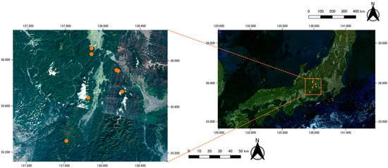
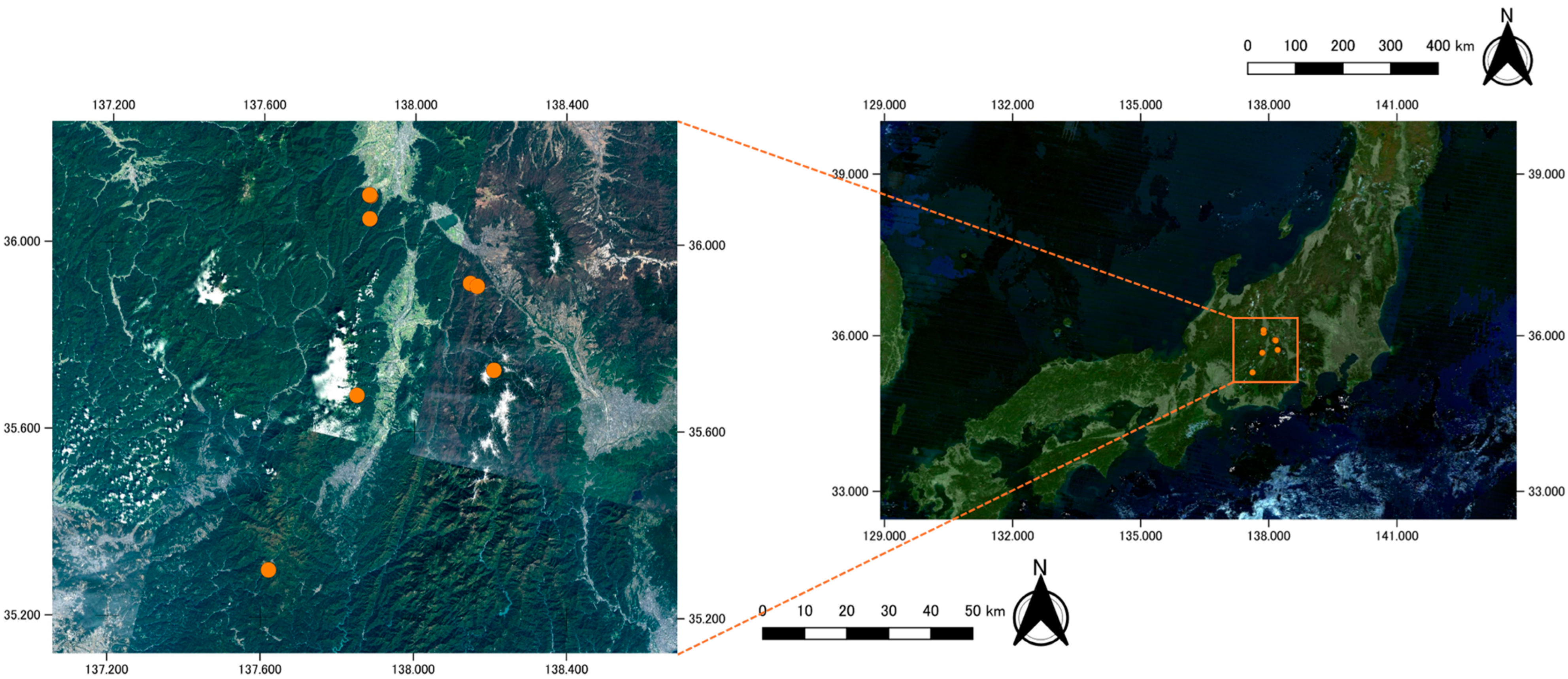
The data were obtained from Nagano Prefecture, Japan. Six study sites were established in Central Japan across an elevation range of 914.0–2081.9 m (35.30–36.11° N, 137.62–138.21° E) (Figure 1, Figure S1). All sites were located within forested land cover. This selection captured the thermal variation driven by elevation and microtopography in snow-influenced environments. The measurements at Seba formed a dense cluster within a single forest stand between 914 and 1035 m. The remaining five sites were measured at a single point to provide broader spatial coverage (Table 1). This uneven design reflects site accessibility and the availability of long-term records provided by the KOA Corporation at Seba; it is a spatial sampling limitation, and site-level validation results are therefore also reported (Section 2.4).
Figure 1.
Location of the study area. The right panel shows the broader location of the study region within Japan. The left panel shows a magnified view of the study region (orange rectangle in the right panel), showing the locations of the six forested sites (orange circles; the 14 points at Seba form two groups about 5 km apart, and Yamamuro and Zatosawa, about 2 km apart, appear as two adjacent circles, so seven circles represent the six sites) in the mountainous terrain of Central Japan, where the air and soil temperatures were measured.
Table 1.
Overview of the study sites.
2.2. Soil and Air Temperature Observations and Data Processing
The air and soil temperatures were recorded at 19 points (Table 2). Fourteen data loggers were installed at different elevations and soil depths in the Seba area. The air temperature was measured at approximately 1.5 m above the ground surface using temperature data loggers (TR-5i, T&D Corporation, Matsumoto, Japan). Each air temperature sensor was shielded from direct solar radiation. The soil temperature was measured using temperature probes connected to the same data loggers and buried at depths of 2, 7, or 15 cm. Sensor recording instruments varied among study sites. At the Yotagirigawa, Zatosawa, and Yamamuro sites, the air and soil temperatures were measured using two-channel temperature data loggers (TR-71wb, T&D Corporation, Matsumoto, Japan), with one sensor measuring the air temperature at approximately 1.5 m above the ground surface and the other measuring the soil temperature at a depth of 2 cm. At the Yukinagesawa site, the air temperature was measured using a temperature and humidity data logger (LR5001, HIOKI E.E. Corporation, Ueda, Japan), where the soil temperature at a depth of 2 cm was measured using a temperature data logger (LR5011, HIOKI E.E. Corporation, Ueda, Japan). The measurements at these four sites were recorded at 10 min intervals. All measurement points, except Yukinagesawa, were located within forests, where the ground surface was shaded from direct solar radiation by the canopy. The Yukinagesawa measurement point was located at the forest edge adjacent to an avalanche-disturbed area, where the ground surface was occasionally exposed to direct solar radiation. The measurement intervals in the Seba area varied among the loggers, resulting in an overall recording interval of 10–60 min across study sites.
Table 2.
Logger identity, sensor depth, and observation period at each measurement point. IDs 4, 7, and 9 (15 cm) and ID 17 (no snow-free season data) were not used for modeling.
Sub-daily measurements were aggregated into the daily maximum, minimum, and mean air temperature and soil temperature for each sensor and calendar day. Daily values were retained only when at least half of the expected sub-daily records were available for both variables. The days that did not meet this criterion were treated as missing data. Readings outside −40 to 50 °C were discarded as physically implausible. At the Yukinagesawa site (2082 m), where the ground surface was occasionally exposed to direct solar radiation, soil temperatures exceeding 28 °C were recorded in May 2023. Because these values were likely caused by the direct solar heating of the sensor and did not represent the soil temperature, they were discarded. Seasonal snowpack holds the near-surface soil temperature close to 0 °C for extended periods. Therefore, we retained the soil temperature near 0 °C during the snow-covered season as valid observations. These days were used to describe the air–soil relationship but were excluded from model training. The number of missing days after data processing is presented in Table 2.
2.3. Acquisition of 1 km Mesh Weather Data
The Agro-Meteorological Grid Square Data System, NARO [37] (https://amu.rd.naro.go.jp/wiki_open/, (accessed on 26 August, 2026)) was used as the gridded meteorological dataset (AMD); it provides daily meteorological variables on a 1 km grid covering Japan, constructed from observed, forecasted, and climatic normal data. The daily mean, maximum, and minimum air temperatures were extracted for the grid cell containing each measurement point, over the observation period of that point, extended seven days earlier so that lagged predictors could be computed without loss at the start of each record. The representative elevation of each grid cell was obtained from the AMD elevation layer. Because a single AMD value represents an entire 1 km cell, the representative elevation of a cell generally differs from that of the sensor within it. Therefore, the elevation-adjusted air temperature was calculated as
where zcell is the representative elevation of the grid cell, zsensor is the elevation of the measurement point, and Γ is the environmental lapse rate, set to 0.006 °C/m. Both the raw and the elevation-adjusted values were used as model inputs and compared. For the spatial prediction, the daily mean air temperature was extracted for every AMD grid cell within the five rectangular areas surrounding the measurement points, and cell elevations were obtained from a 10 m digital elevation model (DEM) provided by the Geospatial Information Authority (GSI) of Japan (https://www.gsi.go.jp/kiban/, (accessed on 15 August, 2026)).
Tadj = TAMD + Γ(zcell − zsensor)
2.4. Soil Temperature Prediction Model Using Random Forest
The daily mean soil temperature was predicted using a random forest model [38] implemented in the randomForest package [39] in R (version 4.5.0; R Core Team). The explanatory variables were the daily mean air temperature on the current day and from the preceding one to seven days (lags 0–7). The model was trained in the snow-free season, defined as 1 May to 30 November. To reduce the influence of snow cover on the air–soil thermal linkage during model training, days with a soil temperature < 0 °C were excluded. This filter removed 18 site-days (approximately 0.3% of the dataset), all between 16 and 30 November at Yukinagesawa and Zatosawa. Because the model was trained only on snow-free conditions, its scope of applicability is limited to the snow-free season. Maps were produced only for June–October, when the study areas are normally snow-free. Because adjacent days were strongly autocorrelated, lagged predictors were computed only within continuous observation segments and never across missing data segments. Moreover, days for which a full lag window was unavailable were excluded. Yotagirigawa provided no data during the May–November period, and the three 15 cm sensors (IDs 4, 7, and 9) were excluded because they operated only in 2025, each co-located with a 7 cm sensor (IDs 5, 6, and 8) and sharing the same air temperature record, so that a depth effect could not be estimated independently of the site. This yielded 5526 site-days from the 15 measurement points (7 cm depth at 11 Seba points and 2 cm depth at four non-Seba points). Because the sensor depth differed between Seba and the other sites, depth was confounded by site. The 2 cm and 7 cm records were therefore pooled as a single response variable without a depth predictor, so that the model could be applied with the gridded air temperature alone; the predictions represent the near-surface (2–7 cm) soil temperature. To examine whether combining depths biased the predictions, we trained separate models for 2 cm and 7 cm points using cross-site validation. These depth-specific models were compared with the combined model. Additionally, a linear regression model using only the same-day and previous-day air temperatures (lags 0 and 1) was evaluated under the same cross-validation schemes.
Three models were compared, differing only in terms of the source of the air temperature: observation, raw AMD, and elevation-adjusted values. The elevation values were obtained by applying a lapse rate of 0.006 °C/m to the difference between the representative of each AMD mesh and the elevation of the target location. Forests of 500 trees were grown for validation and of 1000 trees for the final model, with the number of variables tried at each split set to one-third of the number of predictors. Model transferability was assessed using two grouped cross-validations (Figure S2). In the cross-site validation, each measurement point was withheld in turn (15 times; the remaining Seba points stayed in the training data when one Seba point was withheld), and, in the cross-period validation, each calendar year was withheld in turn (nine times), with some loggers covering only parts of certain years. In addition, leave-one-site-out validation was applied to assess transferability to a new site, in which all points of a site, including all 11 Seba points, were withheld together (five folds). Predictions from all withheld folds were pooled before computing the coefficient of determination (R2), root mean square error (RMSE), and mean absolute error (MAE), so that points contributing more observations were weighted by their data volume. Because the pooled scores were weighted toward sites with long records, and the other Seba points remained in the training data in point-level folds, n, R2, the RMSE, the MAE, and the mean bias (mean of predicted minus observed values) were also computed for each fold (Table S1).
Variable importance was evaluated using the permutation importance within each excluded fold. Each predictor was randomly shuffled ten times and the resulting mean decrease in R2 was recorded. These values were then averaged across folds, and their standard errors were calculated. Given the collinearity among lagged air temperatures, importance scores represent the collective contribution of the recent thermal history rather than strictly independent daily effects.
To map the soil temperature, the final model driven by the elevation-adjusted air temperature was applied to a 10 m grid. For each 10 m cell, the AMD air temperature of the mesh containing the cell was corrected by applying the same lapse rate to the elevation difference between the mesh’s representative elevation and the cell elevation derived from the 10 m DEM, and the corrected air temperatures for lags 0–7 were input to the model. The 10 m grid reflects the resolution of the DEM. Spatial variation within each 1 km mesh came solely from elevation adjustment, and validation was performed only at observation points. Cells above the highest training point (2082 m) or outside forests lay outside the conditions represented in the training data; because a random forest cannot predict beyond the range of its training targets, the predictions for these cells are extrapolations of unknown accuracy.
3. Results
3.1. Predicting Soil Temperature Using In Situ Air Temperature
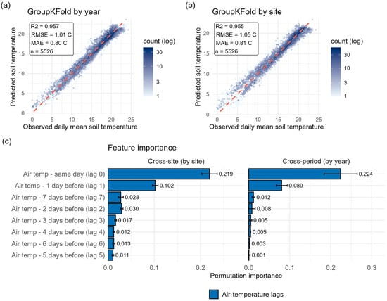
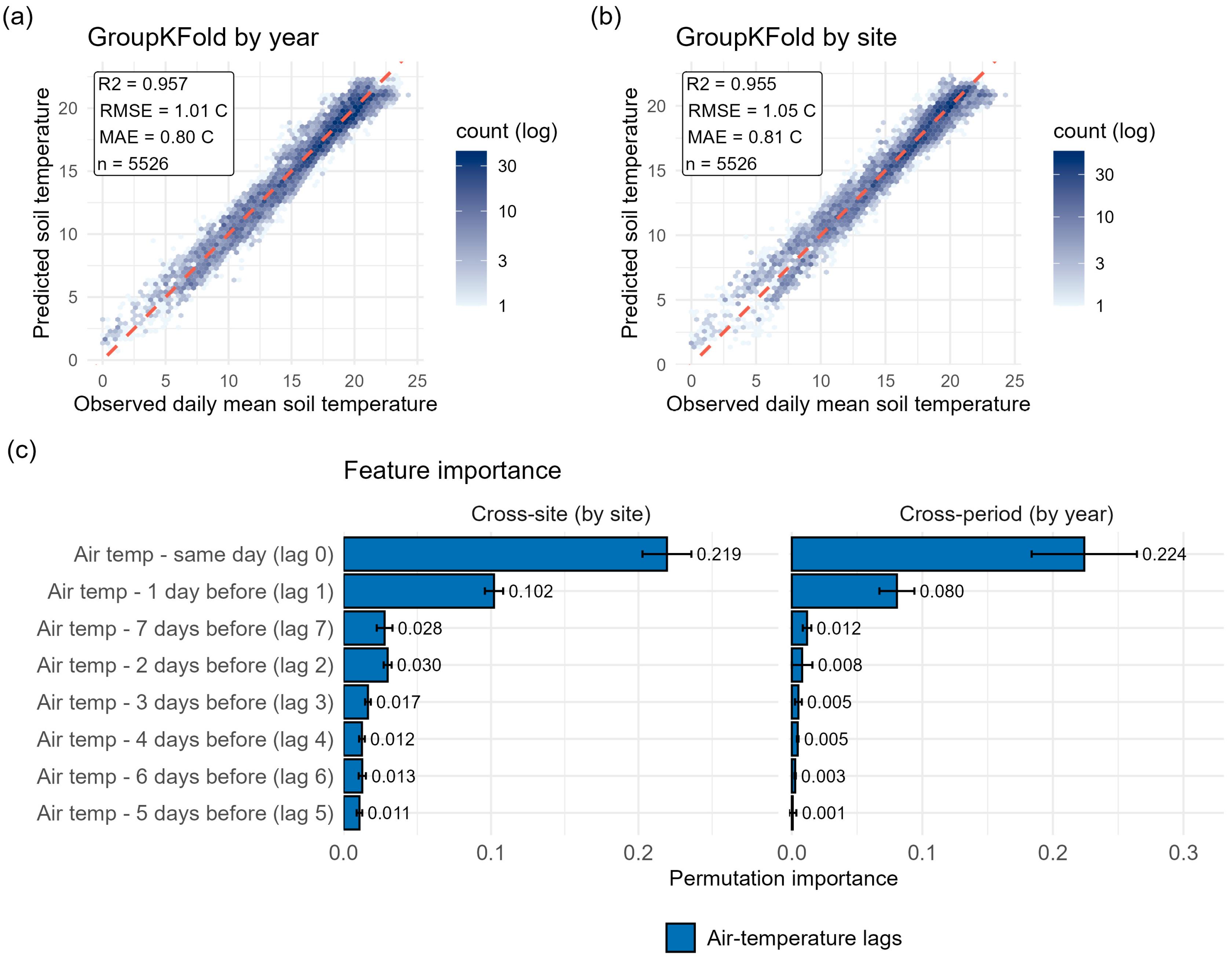
The predicted and observed daily mean soil temperatures agreed closely in both validations using random forest models (Figure 2a,b). The pooled cross-period validation showed R2 = 0.958, RMSE = 1.01 °C, and MAE = 0.79 °C, whereas the pooled cross-site validation also showed R2 = 0.955, RMSE = 1.05 °C, and MAE = 0.81 °C. The point-level RMSE ranged from 0.21 to 1.88 °C, the MAE from 0.16 to 1.68 °C, and the bias from −1.16 to +0.96 °C (Table S1). Because the other Seba points remained in the training data when one Seba point was withheld, the mean point-level RMSE was lower for the 11 Seba points (0.68 °C) than for the four other points (1.18 °C; RMSE 1.08–1.39 °C, MAE 0.88–1.19 °C, bias −1.16 to +0.30 °C). When all points of a site were withheld together (leave-one-site-out validation), the site-level RMSE ranged from 1.07 to 1.53 °C and the pooled RMSE was 1.30 °C (R2 = 0.936); withholding Seba as a whole gave the largest error (RMSE = 1.53 °C, bias = +0.67 °C; Table 3). Permutation importance was concentrated in the shortest air temperature lags (Figure 2c). Under cross-site validation, the same-day air temperature was the largest contributing factor (0.222), followed by the air temperature of the previous day (0.099). All the remaining lags contributed 0.029 or less. The cross-period validation shows the same order for the two leading predictors (0.233 and 0.081). A linear regression model using only lags 0 and 1 resulted in RMSEs of 1.27 °C (cross-site) and 1.20 °C (cross-period), which were approximately 0.2 °C higher than those of the random forest model (Table S3); under leave-one-site-out validation, the difference narrowed to 0.04 °C (1.34 vs. 1.30 °C; Table S2). Furthermore, the combined model showed almost no depth-dependent bias (+0.06 °C at 2 cm and +0.07 °C at 7 cm), and depth-specific models yielded similar RMSEs (2 cm: 1.16 vs. 1.16 °C; 7 cm: 0.73 vs. 0.81 °C; Table S4), indicating that pooling the two depths introduced no substantial depth-related bias. The predicted values show the seasonal course of the observed air temperature at the low, middle, and high elevation points (Figure S3).
Figure 2.
Random forest prediction of daily mean soil temperature from in situ air temperature. (a,b) Predicted versus observed daily mean soil temperature under a (a) cross-validation grouped by year and (b) by site. Hexagonal shading indicates the observed count (log scale), and the dashed line represents a 1:1 relationship. The insert in each panel reports the coefficient of determination (R2), RMSE, MAE, and number of daily observations. (c) Permutation importance of the air temperature lag features (lags 0–7) under the cross-site (left) and cross-period (right) schemes.
Table 3.
Site-level results of the leave-one-site-out validation with in situ air temperature (all points of the withheld site excluded from training).
3.2. Comparison of In Situ Data and 1 km Mesh Temperature Data
The 1 km mesh air temperature agreed closely with the observed air temperature (Figure S4a). The site-level offset was explained by the difference between the 1 km mesh cell elevation and sensor elevation (Figure S4b; slope = −0.0079 °C/m, R2 = 0.794, p < 0.001) at a rate close to the environmental lapse rate. At Seba, where 14 measurement points fell within a single 1 km grid cell, the observed soil temperature was separated according to the sensor elevation, while the mesh value was identical for all of them (Figure S5), and elevation adjustment reduced the offset where the mismatch was large. By contrast, at some sites, the raw values were nearly unbiased (Figure S4c).
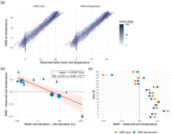
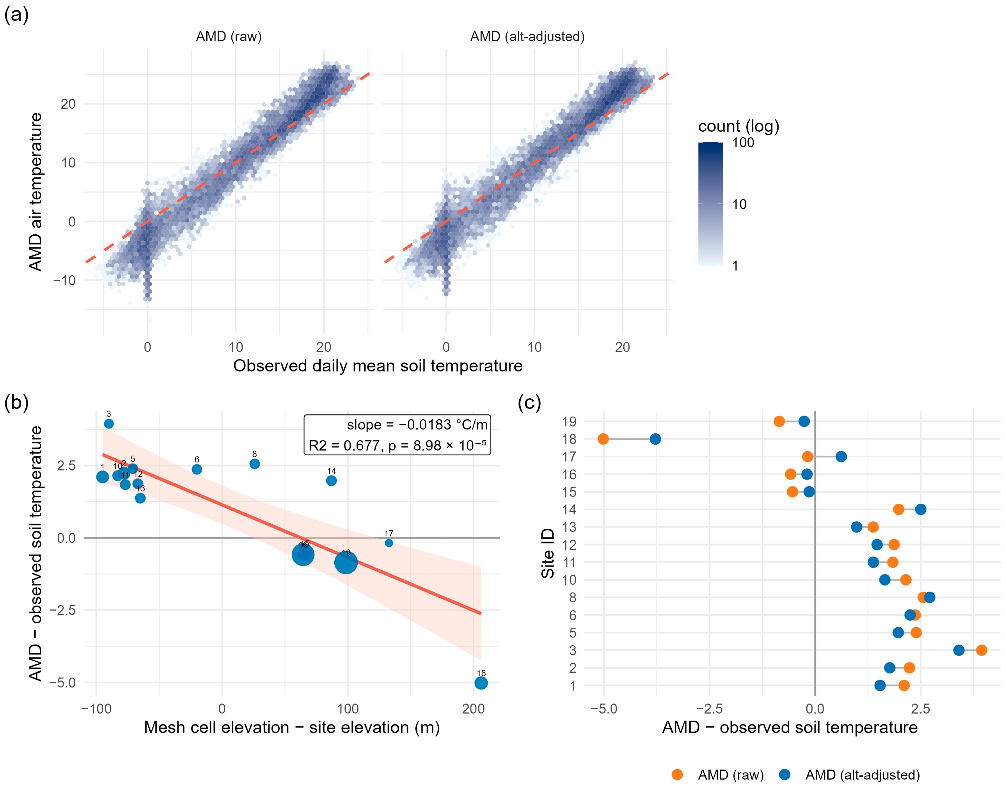
The 1 km mesh air temperature deviated from the observed soil temperature (Figure 3a). A dense cluster of observations near 0 °C reflected the snow-covered period, during which the soil temperatures remained close to 0 °C, while the mesh air temperature fell to −10 °C or below (Figure S6). The site-level offset between the mesh and observed soil temperature was also related to the difference in elevation (Figure 3b; slope = −0.0183 °C/m, R2 = 0.677, p < 0.001). Sites located above their cell elevation showed offsets of +1.4 to +3.9 °C, whereas the highest site, 206 m below its cell elevation, showed an offset of −5.0 °C. The fitted slope was approximately twice the environmental lapse rate. The elevation adjustment shifted the site-level offsets but did not remove them (Figure 3c).
Figure 3.
Comparison of 1 km mesh air temperature with observed soil temperature. (a) Observed daily mean soil temperature and mesh air temperature, raw and elevation-adjusted. Hexagon shading indicates observed count (log scale); the dashed line represents a 1:1 relationship. The data points near 0 °C correspond to snow cover days, which were excluded from model training. (b) Site-level offset versus elevation difference between mesh and sensors. Point size is proportional to site-days. The line denotes a linear fit with a 95% confidence band. (c) Site-level offsets before and after elevation adjustment.
3.3. Predicting Soil Temperatures Using 1 km Mesh Temperature Data
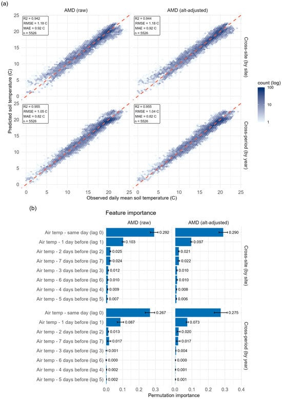
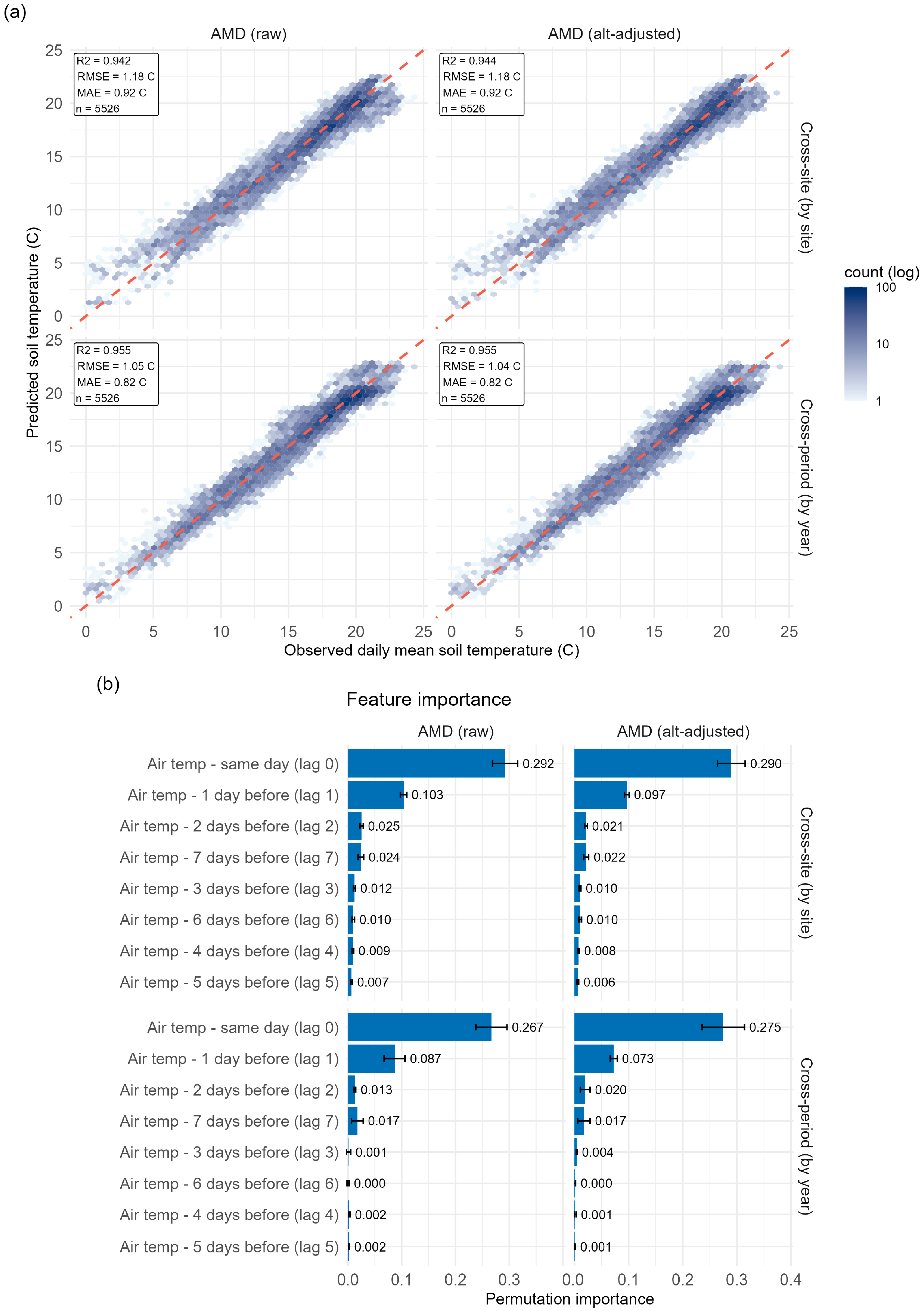
The predicted and observed daily mean soil temperatures were similar under both validations using the random forest model with 1 km mesh air temperatures (Figure 4a). Cross-period validation showed R2 = 0.955, RMSE = 1.04–1.05, and MAE = 0.82, whereas cross-site validation showed R2 = 0.942–0.944, RMSE = 1.18, and MAE = 0.92. Elevation adjustment slightly improved the predictive performance under cross-period validation, reducing the RMSE from 1.05 to 1.04, but had a negligible effect under cross-site validation. Permutation importance was again concentrated in the shortest air temperature lag (Figure 4b). Under cross-site validation, the same-day air temperature was the largest contributing factor (0.290–0.292), followed by the air temperature of the previous day (0.097–0.103). All remaining lags contributed 0.025 or less. The cross-period validation showed the same order for the two leading predictors (0.267–0.275 and 0.073–0.087, respectively).
Figure 4.
Random forest prediction of soil temperature from 1 km mesh air temperature. (a) Observed versus predicted values for holding-out folds, pooled, for raw and elevation-adjusted mesh air temperature under cross-site (by site) cross-period (by year) validation. Hexagon shading indicates observed count (log scale); the dashed line represents a 1:1 relationship. (b) Permutation importance under the same four combinations, given as the mean decrease in R2 across folds.
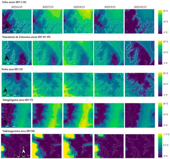
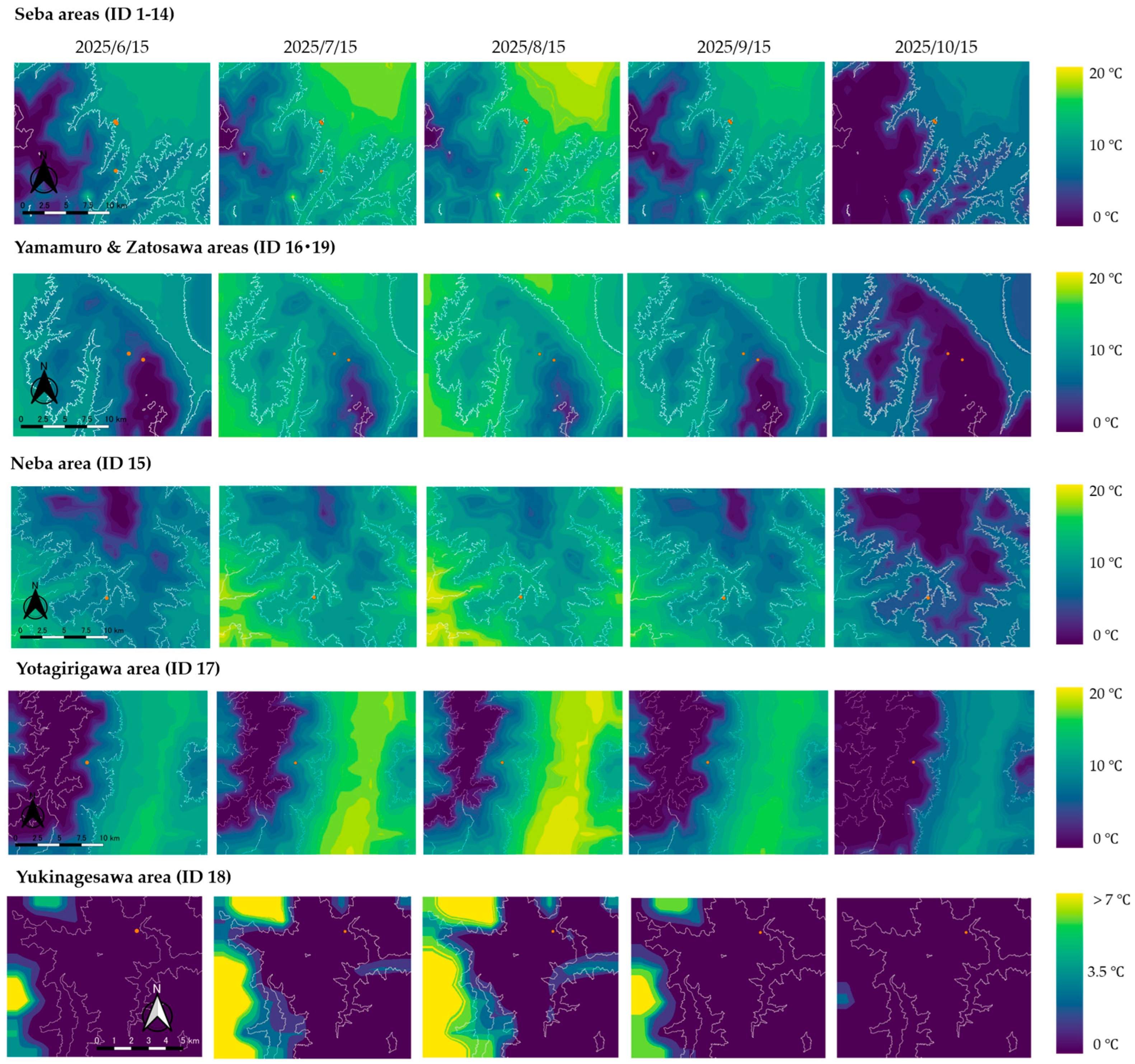
3.4. Spatial Distribution of Predicted Soil Temperature
The daily mean soil temperature on the 15th of each month was predicted across the five areas from June to October 2025 (Figure 5) using a random forest model. The predictions relied only on AMD air temperature data and 10 m digital elevation data from GSI. Soil temperatures exhibited clear seasonal variations across all areas, peaking in August and declining to their lowest values by October, the final month of the mapped period. In Seba, Neba, and Yotagirigawa, the mean temperatures peaked in August at 12.3, 12.2, and 12.2 °C, respectively, declining to 4.7–5.2 °C in October (Table S5). Yamamuro and Zatosawa followed a similar pattern. Lower temperatures were consistently observed at higher elevations. Yukinagesawa recorded lower values, averaging 2.6 °C in August and 0.8 °C in October, and was the only area where the mean predicted temperature remained below 3 °C throughout the period. As described in Section 2.4, these maps were not validated away from the monitoring points; they illustrate the workflow rather than providing validated estimates for unmonitored cells.
Figure 5.
Mapped soil temperature predicted from 1 km mesh air temperature. Predicted snow-free season daily mean near-surface (2–7 cm) soil temperature, estimated with the random forest driven by the 1 km mesh air temperature, from 15 June to 15 October 2025, for each study area. The orange points indicate the soil and air temperature sensors; overlapping points represent sensors installed at the same or nearby locations (e.g., co-located sensors at different depths at Seba), and white lines are contour lines at 1000 m intervals. Color scales were set independently for each area. The scale bars represent 10 km for the upper four rows and 5 km for the Yukinagesawa area. The 10 m grid reflects the DEM resolution, and the maps have not been validated away from the sensors.
4. Discussion
This study investigated whether an empirical model based on air temperature data could predict the daily mean soil temperature. The results show that, across middle-to-high-elevation sites in Central Japan, the soil temperature can be predicted with high accuracy only from the air temperature outside snow-covered periods.
The observed data model showed high accuracy (Figure 2). This result indicates that a monitoring network spanning five sites and up to eight years of records can achieve the accuracy range reported for other tree-based soil temperature models. Similar results have been reported in multiple studies conducted across different regions. Random forest and gradient-boosted models trained across seven Chinese climate areas reached R2 = 0.96–0.97 and RMSE = 1.73–1.99 at the soil surface [35]. Another study indicated that a nine-depth random forest for the Tibetan Plateau’s Three River region reached RMSEs ranging from 1.7 near the surface to 2.3 °C at 160 cm [36]. These studies, however, used additional predictors such as the soil depth, radiation, humidity, and wind and different validation strategies; their RMSE values are therefore not directly comparable with those of this study, although the errors fall within a similar range. Unlike earlier approaches to the spatially distributed soil temperature that relied on topographic or surface cover variables [12,13], the present model uses only the air temperature, which makes transferability across sites the critical test. The air temperature was consistently the primary predictor of the soil temperature, similar to other machine learning models across diverse climates [40]. Across all models, the same-day air temperature and its one-day lag accounted for 74–91% of the total importance assigned to lags 0–7. This result is consistent with heat transfer theory, which represents soil heat propagation as a damped phased-lagged response to surface forcing [13].
Replacing the observed air temperature with 1 km AMD data caused little loss of accuracy. However, the variable importance in the AMD models shifted further toward the same-day air temperatures. This shift suggests that spatial averaging over 1 km grid cells smooths the local short-term variability that lag terms would otherwise capture. The AMD air temperature closely tracked the observed air temperature, with a site-level offset scaled with elevation at close to the environmental lapse rate. Its divergence from the observed soil temperature, however, was larger as the site-level offset scaled with the elevation difference at approximately −0.018 °C/m, which is more than twice the environmental lapse rate. The standard elevation adjustment shifted these offsets without resolving them, yielding a negligible improvement in the cross-site RMSE.
The effect of the random forest trained depends on the validation scheme. The cross-site RMSE remained essentially unchanged, whereas the cross-period RMSE improved slightly. Therefore, these results indicate that elevation adjustment corrects the systematic site-level air temperature bias more effectively than it corrects the soil temperature transferability differences between sites. This pattern is consistent with elevation acting as a proxy for several covarying drivers, including snow cover, the canopy, and the radiation load, rather than a single physical correction term. The accuracy of this approach was also affected by the accuracy of the AMD data. AMD is the least constrained in complex terrain and at high elevations, where AMeDAS stations are sparse. Therefore, the input error is expected to be largest in settings where soil temperature prediction is most challenging.
Snowpack insulation caused the largest single divergence between the air and soil temperatures. The soil temperature stayed near 0 °C, while the air temperature fell to −10 °C or below. The air temperature input could not directly represent this insulation. Random forest can learn this insulation effect only empirically and only when the training data span snow-covered periods. This limitation is inherent in any air temperature-based framework and is not specific to the random forest. Because snow cover weakens the relationship between the air and soil temperatures, this model is applicable only to the snow-free period.
This study had several limitations. First, spatial replication was uneven. Eleven of the 15 modeled points were in a single forest stand at Seba (914–1035 m), whereas each of the other four sites had one point; three of these were at higher elevations, while Neba (954 m) lay within the Seba range. Consequently, the point-level cross-site score mainly reflects interpolation within Seba, and the leave-one-site-out results (site-level RMSE 1.07–1.53 °C; Table 3) are the more appropriate indication of the uncertainty expected at a new forested site within the sampled elevation range (914–2082 m). Although more rigorous than random cross-validation [41], these errors reflect the features of individual sites rather than a systematic elevation gradient, and transferability to unmonitored terrain above the highest training point, in non-forested settings or in other mountain ranges, has not been tested. Second, the number of days used for modeling varied from 61 to 1681 per point. Cross-period validation confounds the interannual climate variability with incomplete seasonal sampling. In addition, daily values were screened only by the number of available sub-daily records. The distribution of missing records within each day was not assessed; daily means on days with uneven coverage may be biased. Third, because the sensor depth coincided with the site, the depth comparison cannot fully separate depth effects from site effects; thermal damping and lag increase with depth, so the model should not be applied to depths outside the 2–7 cm range represented in the training data. Finally, all the areas were located on forested land in Central Japan. However, the model’s transferability to non-forested, exposed, or geologically distinct mountain environments remains untested.
The model achieved this accuracy from the air temperature and elevation alone, with errors in a similar range to those of more input-intensive models in previous studies [38,39]. The required inputs, the 1 km AMD data and 10 m DEM, are available nationwide for Japan. As a demonstration, the model produced spatially continuous snow-free season soil temperature maps for five study areas (Figure 5), although their spatial accuracy away from logger sites has not yet been validated. As elevation-dependent warming accelerates, scalable soil temperature monitoring is increasingly required in mountains [9]. Using open data, this approach may help to link sparse reference sites to ungauged mountain terrain, which is consistent with digital soil mapping efforts across Japan [42]. Future work should validate spatial predictions away from logger sites, extend the training networks to non-forested and high-elevation sites, and incorporate snow cover indicators. Such expanded models could then be applied to historical reconstructions and future climate projections. Coupled with snow cover information, such estimates could eventually inform assessments of freeze–thaw activity and its role in soil erosion in mountain catchments.
5. Conclusions
This study showed that the daily mean near-surface (2–7 cm) soil temperature in the snow-free season at forested mountain sites in Central Japan can be predicted from the current and lagged air temperature alone. With the in situ air temperature, the pooled RMSE was about 1.0 °C under point-level cross-site and cross-period validation and 1.30 °C when entire sites were withheld (site-level RMSE 1.07–1.53 °C); with the 1 km gridded air temperature, the cross-site RMSE was 1.18 °C. The lapse rate adjustment of the gridded data did not remove the site-level bias, indicating that elevation acts as a proxy for several covarying drivers. Because 11 of the 15 modeled points were in a single stand, these results apply most directly to forested sites within the sampled elevation range. In addition, the 2 cm and 7 cm records were combined, and, because the sensor depth coincided with the site, depth-specific effects could not be separated. Therefore, the results apply only to the near-surface (2–7 cm) soil temperature. The 10 m maps are presented as an example of applying the model. Their accuracy at locations without measurements has not been validated. The model applies only to the snow-free season and should not be used for snow-covered periods. Extending the approach to the snow-covered season will require snow cover predictors, and denser sampling at high elevations and in non-forested terrain is needed. From a sustainability perspective, the use of freely available nationwide data may reduce the reliance on dense sensor networks and the cost and effort of monitoring soil thermal conditions in mountain forests. Once validated more widely, such estimates could support sustainable forest management and climate change adaptation planning that accounts for soil biological activity in a warming climate.
Supplementary Materials
The following supporting information can be downloaded at https://www.mdpi.com/article/10.3390/su182111293/s1. Figure S1: Elevation of the study region and locations of the measurement points; Figure S2: Grouped cross-validation schemes; Figure S3: Time series of observed and 1 km mesh temperature at three measurement points; Figure S4: Comparison of 1km mesh air temperature with observed air temperature; Figure S5: Soil temperature along with the elevation gradient at Seba area compared with the AMD mesh air temperature; Figure S6: Observed air and soil temperature at Zatosawa from 2017 to 2025; Table S1: Fold-level validation statistics of the random forest model; Table S2: Leave-one-site-out validation statistics; Table S3: Comparison with a linear regression model (lags 0 and 1); Table S4: Validation statistics by sensor depth; Table S5: Predicted soil temperature statistics for each study area.
Author Contributions
Conceptualization, O.W. and K.M.; methodology, O.W. and K.M.; software, K.M.; validation, K.M.; formal analysis, O.W. and K.M.; investigation, O.W. and T.F.; resources, O.W. and T.F.; data curation, O.W., K.M., and T.F.; writing—original draft preparation, K.M.; writing—review and editing, O.W., K.M., and T.F.; visualization, K.M. All authors have read and agreed to the published version of the manuscript.
Funding
This research was partially supported by a JSPS KAKENHI Grant-in-Aid for Scientific Research (C), Grant Number 21K04607.
Institutional Review Board Statement
Not applicable.
Informed Consent Statement
Not applicable.
Data Availability Statement
The datasets presented in this article are not readily available because some of the data used in this study were provided by a third party and are subject to restrictions on their distribution. Requests to access the datasets should be directed to the corresponding author.
Acknowledgments
We thank the KOA Corporation for providing the air and soil temperature data at the Seba site, Shiojiri City, and for their cooperation in the field measurements. During the preparation of this manuscript, the authors used Claude [Opus 5.5; Anthropic] for graphics for the R code. The authors have reviewed and edited the manuscript and take full responsibility for the content of this publication.
Conflicts of Interest
The authors declare no conflicts of interest.
Abbreviations
The following abbreviations are used in this manuscript:
| AMD | Agro-Meteorological Grid Square Data |
| AMeDAS | Automated Meteorological Data Acquisition System |
| DEM | Digital elevation model |
| MAE | Mean absolute error |
| R2 | Coefficient of determination |
| RMSE | Root mean square error |
References
- Knight, J. Scientists’ Warning of the Impacts of Climate Change on Mountains. PeerJ 2022, 10, e14253. [Google Scholar] [CrossRef] [Scilit]
- Marta, S.; Zimmer, A.; Caccianiga, M.; Gobbi, M.; Ambrosini, R.; Azzoni, R.S.; Gili, F.; Pittino, F.; Thuiller, W.; Provenzale, A.; et al. Heterogeneous Changes of Soil Microclimate in High Mountains and Glacier Forelands. Nat. Commun. 2023, 14, 5306. [Google Scholar] [CrossRef] [Scilit]
- Zhao, H.; Sun, S.; Song, C.; Lin, S.; Hu, Z.; Meng, X.; Li, J.; Guo, L.; Wang, G. Freeze-Thaw-Driven Soil Moisture Return Significantly Contributes to Spring Phenology on the Warming Qinghai-Tibet Plateau. Nat. Commun. 2026, 17, 3981. [Google Scholar] [CrossRef] [Scilit]
- Zhao, Y.; Zheng, C.; Gelfan, A.; Watanabe, K.; Liu, H.; Wright, S.; Wu, X.; Quinton, W.; Wang, Y.; Yi, S.; et al. Frozen Soil Hydrological Processes and Their Effects: A Review and Synthesis. Rev. Geophys. 2026, 64, e2024RG000839. [Google Scholar] [CrossRef] [Scilit]
- Fernández-Pascual, E.; Carta, A.; Mondoni, A.; Cavieres, L.A.; Rosbakh, S.; Venn, S.; Satyanti, A.; Guja, L.; Briceño, V.F.; Vandelook, F.; et al. The Seed Germination Spectrum of Alpine Plants: A Global Meta-analysis. New Phytol. 2021, 229, 3573–3586. [Google Scholar] [CrossRef] [Scilit]
- Espinosa del Alba, C.; Fernández-Pascual, E.; Jiménez-Alfaro, B. Microclimatic Variation Regulates Seed Germination Phenology in Alpine Plant Communities. J. Ecol. 2025, 113, 249–262. [Google Scholar] [CrossRef] [Scilit]
- Ivashchenko, K.; Sushko, S.; Selezneva, A.; Ananyeva, N.; Zhuravleva, A.; Kudeyarov, V.; Makarov, M.; Blagodatsky, S. Soil Microbial Activity along an Altitudinal Gradient: Vegetation as a Main Driver beyond Topographic and Edaphic Factors. Appl. Soil Ecol. 2021, 168, 104197. [Google Scholar] [CrossRef] [Scilit]
- Zhang, T. Influence of the Seasonal Snow Cover on the Ground Thermal Regime: An Overview. Rev. Geophys. 2005, 43, RG4002. [Google Scholar] [CrossRef] [Scilit]
- Pepin, N.; Bradley, R.S.; Diaz, H.F.; Baraer, M.; Caceres, E.B.; Forsythe, N.; Fowler, H.; Greenwood, G.; Hashmi, M.Z.; Liu, X.D.; et al. Elevation-Dependent Warming in Mountain Regions of the World. Nat. Clim. Change 2015, 5, 424–430. [Google Scholar] [CrossRef] [Scilit]
- Pepin, N.; Apple, M.; Knowles, J.; Terzago, S.; Arnone, E.; Hänchen, L.; Napoli, A.; Potter, E.; Steiner, J.; Williamson, S.N.; et al. Elevation-Dependent Climate Change in Mountain Environments. Nat. Rev. Earth Environ. 2025, 6, 772–788. [Google Scholar] [CrossRef] [Scilit]
- Aalto, J.; le Roux, P.C.; Luoto, M. Vegetation Mediates Soil Temperature and Moisture in Arctic-Alpine Environments. Arct. Antarct. Alp. Res. 2013, 45, 429–439. [Google Scholar] [CrossRef] [Scilit]
- Liang, L.L.; Riveros-Iregui, D.A.; Emanuel, R.E.; McGlynn, B.L. A Simple Framework to Estimate Distributed Soil Temperature from Discrete Air Temperature Measurements in Data-scarce Regions. J. Geophys. Res. Atmos. 2014, 119, 407–417. [Google Scholar] [CrossRef] [Scilit]
- Kang, S.; Kim, S.; Oh, S.; Lee, D. Predicting Spatial and Temporal Patterns of Soil Temperature Based on Topography, Surface Cover and Air Temperature. For. Ecol. Manag. 2000, 136, 173–184. [Google Scholar] [CrossRef] [Scilit]
- Paul, K.I.; Polglase, P.J.; Smethurst, P.J.; O’Connell, A.M.; Carlyle, C.J.; Khanna, P.K. Soil Temperature under Forests: A Simple Model for Predicting Soil Temperature under a Range of Forest Types. Agric. For. Meteorol. 2004, 121, 167–182. [Google Scholar] [CrossRef] [Scilit]
- Lei, S.; Daniels, J.L.; Bian, Z.; Wainaina, N. Improved Soil Temperature Modeling. Environ. Earth Sci. 2011, 62, 1123–1130. [Google Scholar] [CrossRef] [Scilit]
- Svensson, M.; Jansson, P.-E.; Gustafsson, D.; Kleja, D.B.; Langvall, O.; Lindroth, A. Bayesian Calibration of a Model Describing Carbon, Water and Heat Fluxes for a Swedish Boreal Forest Stand. Ecol. Modell. 2008, 213, 331–344. [Google Scholar] [CrossRef] [Scilit]
- Dolschak, K.; Gartner, K.; Berger, T.W. A New Approach to Predict Soil Temperature under Vegetated Surfaces. Model. Earth Syst. Environ. 2015, 1, 32. [Google Scholar] [CrossRef] [Scilit]
- Hosseinzadeh Talaee, P. Daily Soil Temperature Modeling Using Neuro-Fuzzy Approach. Theor. Appl. Climatol. 2014, 118, 481–489. [Google Scholar] [CrossRef] [Scilit]
- Alizamir, M.; Ahmed, K.O.; Kim, S.; Heddam, S.; Gorgij, A.D.; Chang, S.W. Development of a Robust Daily Soil Temperature Estimation in Semi-Arid Continental Climate Using Meteorological Predictors Based on Computational Intelligent Paradigms. PLoS ONE 2023, 18, e0293751. [Google Scholar] [CrossRef] [Scilit]
- Farhangmehr, V.; Cobo, J.H.; Mohammadian, A.; Payeur, P.; Shirkhani, H.; Imanian, H. A Convolutional Neural Network Model for Soil Temperature Prediction under Ordinary and Hot Weather Conditions: Comparison with a Multilayer Perceptron Model. Sustainability 2023, 15, 7897. [Google Scholar] [CrossRef] [Scilit]
- Farhangmehr, V.; Imanian, H.; Mohammadian, A.; Cobo, J.H.; Shirkhani, H.; Payeur, P. A Spatiotemporal CNN-LSTM Deep Learning Model for Predicting Soil Temperature in Diverse Large-Scale Regional Climates. Sci. Total Environ. 2025, 968, 178901. [Google Scholar] [CrossRef] [Scilit]
- Saeidinia, M.; Haghiabi, A.H.; Nazeri Tahroudi, M.; Nasrolahi, A.; De Michele, C. Deep Learning and Vine Copula-Based Sequencing: Approaches under Investigation for Forecasting Soil Temperature Dynamics. Stoch. Environ. Res. Risk Assess. 2025, 39, 4949–4983. [Google Scholar] [CrossRef] [Scilit]
- Hatamiafkoueieh, J.; Heddam, S.; Khoshtinat, S.; Khazaei, S.; Osmani, A.-B.; Nohani, E.; Kiomarzi, M.; Sharafi, E.; Tiefenbacher, J. Enhanced Forecasting of Multi-Step Ahead Daily Soil Temperature Using Advanced Hybrid Vote Algorithm-Based Tree Models. J. Hydroinform. 2023, 25, 2643–2659. [Google Scholar] [CrossRef] [Scilit]
- Yang, L.; Song, R.; Dong, B.; Yin, L.; Fan, Y.; Zhang, B.; Wang, Z.; Wang, Y.; Dong, S. Processing Method of Soil Temperature Time Series and Its Application in Geothermal Heat Flow. Front. Earth Sci. 2022, 10, 910328. [Google Scholar] [CrossRef] [Scilit]
- Tabari, H.; Hosseinzadeh Talaee, P.; Willems, P. Short-Term Forecasting of Soil Temperature Using Artificial Neural Network. Meteorol. Appl. 2015, 22, 576–585. [Google Scholar] [CrossRef] [Scilit]
- Meyer, H.; Reudenbach, C.; Hengl, T.; Katurji, M.; Nauss, T. Improving Performance of Spatio-Temporal Machine Learning Models Using Forward Feature Selection and Target-Oriented Validation. Environ. Model. Softw. 2018, 101, 1–9. [Google Scholar] [CrossRef] [Scilit]
- Araghi, A.; Mousavi-Baygi, M.; Adamowski, J.; Martinez, C.; van der Ploeg, M. Forecasting Soil Temperature Based on Surface Air Temperature Using a Wavelet Artificial Neural Network. Meteorol. Appl. 2017, 24, 603–611. [Google Scholar] [CrossRef] [Scilit]
- Xing, L.; Li, L.; Gong, J.; Ren, C.; Liu, J.; Chen, H. Daily Soil Temperatures Predictions for Various Climates in United States Using Data-Driven Model. Energy 2018, 160, 430–440. [Google Scholar] [CrossRef] [Scilit]
- Olds, B.M.; Wolf, M.A.; Goeking, S.A.; Brooks, P.D. Quantifying the Influence of Vegetation on Net Snow Accumulation Across Elevations, Aspects and During Years With High and Low Snowfall. Ecohydrology 2026, 19, e70156. [Google Scholar] [CrossRef] [Scilit]
- Rutten, G.; Ensslin, A.; Hemp, A.; Fischer, M. Vertical and Horizontal Vegetation Structure across Natural and Modified Habitat Types at Mount Kilimanjaro. PLoS ONE 2015, 10, e0138822. [Google Scholar] [CrossRef] [Scilit]
- Lievens, H.; Demuzere, M.; Marshall, H.-P.; Reichle, R.H.; Brucker, L.; Brangers, I.; de Rosnay, P.; Dumont, M.; Girotto, M.; Immerzeel, W.W.; et al. Snow Depth Variability in the Northern Hemisphere Mountains Observed from Space. Nat. Commun. 2019, 10, 4629. [Google Scholar] [CrossRef] [Scilit]
- Chu, Q.; Yan, G.; Qi, J.; Mu, X.; Li, L.; Tong, Y.; Zhou, Y.; Liu, Y.; Xie, D.; Wild, M. Quantitative Analysis of Terrain Reflected Solar Radiation in Snow-Covered Mountains: A Case Study in Southeastern Tibetan Plateau. J. Geophys. Res. Atmos. 2021, 126, e2020JD034294. [Google Scholar] [CrossRef] [Scilit]
- Shahgedanova, M.; Adler, C.; Gebrekirstos, A.; Grau, H.R.; Huggel, C.; Marchant, R.; Pepin, N.; Vanacker, V.; Viviroli, D.; Vuille, M. Mountain Observatories: Status and Prospects for Enhancing and Connecting a Global Community. Mt. Res. Dev. 2021, 41, A1. [Google Scholar] [CrossRef] [Scilit]
- Broxton, P.; Ehsani, M.R.; Behrangi, A. Improving Mountain Snowpack Estimation Using Machine Learning With Sentinel-1, the Airborne Snow Observatory, and University of Arizona Snowpack Data. Earth Space Sci. 2024, 11, e2023EA002964. [Google Scholar] [CrossRef] [Scilit]
- Dong, J.; Huang, G.; Wu, L.; Liu, F.; Li, S.; Cui, Y.; Wang, Y.; Leng, M.; Wu, J.; Wu, S. Modelling Soil Temperature by Tree-Based Machine Learning Methods in Different Climatic Regions of China. Appl. Sci. 2022, 12, 5088. [Google Scholar] [CrossRef] [Scilit]
- Tan, X.; Luo, S.; Li, H.; Li, Z.; Dong, Q. A Soil Temperature Dataset Based on Random Forest in the Three River Source Region. Sci. Data 2025, 12, 882. [Google Scholar] [CrossRef] [Scilit]
- Ohno, H.; Sasaki, K.; Ohara, G.; Nakazono, K. Development of Grid Square Air Temperature and Precipitation Data Compiled from Observed, Forecasted, and Climatic Normal Data. Clim. Biosph. 2016, 16, 71–79. [Google Scholar] [CrossRef] [Scilit]
- Breiman, L. Random Forests. Mach. Learn. 2001, 45, 5–32. [Google Scholar] [CrossRef] [Scilit]
- Liaw, A.; Wiener, M. Classification and Regression by RandomForest. Forest 2001, 23, 18–22. [Google Scholar]
- Feng, Y.; Cui, N.; Hao, W.; Gao, L.; Gong, D. Estimation of Soil Temperature from Meteorological Data Using Different Machine Learning Models. Geoderma 2019, 338, 67–77. [Google Scholar] [CrossRef] [Scilit]
- Roberts, D.R.; Bahn, V.; Ciuti, S.; Boyce, M.S.; Elith, J.; Guillera-Arroita, G.; Hauenstein, S.; Lahoz-Monfort, J.J.; Schröder, B.; Thuiller, W.; et al. Cross-validation Strategies for Data with Temporal, Spatial, Hierarchical, or Phylogenetic Structure. Ecography 2017, 40, 913–929. [Google Scholar] [CrossRef] [Scilit]
- Yamashita, N.; Ohnuki, Y.; Iwahashi, J.; Imaya, A. National-Scale Mapping of Soil-Thickness Probability in Hilly and Mountainous Areas of Japan Using Legacy and Modern Soil Survey. Geoderma 2024, 446, 116896. [Google Scholar] [CrossRef] [Scilit]

Disclaimer/Publisher’s Note: The statements, opinions and data contained in all publications are solely those of the individual author(s) and contributor(s) and not of MDPI and/or the editor(s). MDPI and/or the editor(s) disclaim responsibility for any injury to people or property resulting from any ideas, methods, instructions or products referred to in the content. |
© 2026 by the authors. Licensee MDPI, Basel, Switzerland. This article is an open access article distributed under the terms and conditions of the Creative Commons Attribution (CC BY) license.