


Abstract
China tests sustainability policies, from low-carbon and sponge cities to new-energy-vehicle promotion, in city pilot programmes, and their effects are usually estimated one programme at a time with staggered difference-in-differences (DID) designs. The programmes, however, overlap. Of 297 cities, 169 hosted two or more of ten national programmes by 2022, and 75–95% of each programme’s treated city-years overlapped with another. Monte Carlo simulations calibrated to city PM2.5, with known effects for every programme, show that this overlap contaminates DID evaluations. When each co-located programme is as effective as the focal one, two-way fixed effects, event-study and heterogeneity-robust estimators overstate the focal effect by a median 78–139%. A programme with no effect is found significant in 11–22% of simulated evaluations when co-located effects are small (0.6%), and in 71–100% in a stress test that sets each to the median of three verifiable published estimates (−3.45%). Adding dummies for the other programmes, the usual robustness check, reverses the bias, and pretrend tests rarely detect the problem. Because the contamination is a weighted sum of the other programmes’ effects, with weights fixed by the treatment pattern, these weights can be computed before outcome data are examined; we provide code and a checklist for evaluations of sustainability policies.
1. Introduction
China’s central ministries routinely test new policies in designated pilot cities before extending them nationwide [1,2]. Low-carbon cities, smart cities, e-commerce demonstration cities, sponge cities, new-energy-vehicle promotion cities and many similar programmes have each been evaluated in a large number of staggered difference-in-differences (DID) studies (e.g., [3]). Many of these programmes, from low-carbon and sponge cities to new-energy-vehicle promotion, are instruments of China’s environmental and low-carbon policy, and their evaluations are meant to inform which measures are extended nationwide. These studies compare cities selected in successive batches with cities not yet or never selected. The appeal is clear: the batches look like a quasi-natural experiment, and city-level outcomes are easy to obtain.
The difficulty is that the experiments are not run one at a time. Programmes are assigned by different ministries, but they tend to land in the same places: provincial capitals, sub-provincial cities and the coastal east. In the database we assemble for ten national programmes, 169 of 297 cities hosted two or more programmes by 2022, and one city hosted all ten. Between 75% and 95% of each programme’s treated city-years were also treated by at least one other programme. A DID estimate for one pilot therefore compares cities that differ in several pilots at once. When one programme is the focus of an evaluation, we call the other programmes co-located programmes, a treated city-year that also hosts one of them overlapped, and the part of the estimate that reflects their effects contamination.
The problem is not peculiar to China. Evaluators routinely estimate the effect of one programme in jurisdictions exposed to several: US states adopt marijuana policies as bundles that keep changing after adoption [4], state policies co-occur in ways that complicate the estimation of any one of them [5], and housing price controls are introduced, tightened, relaxed and abolished in sequence [6]. Chinese city pilots are an unusually clear case: the programmes are numerous, their designation dates are public, and the overlap among them can be measured exactly.
Applied researchers know this. A robustness check titled “excluding the interference of other policies” has become a standard part of the genre. In ten recent open access studies whose full texts we examined, seven added dummy variables for other pilots or policy events to the regression and three deleted cities that hosted other pilots. To our knowledge, whether these checks work has not been examined systematically.
The recent econometric literature on DID does not settle the question, because it addresses a different problem. It shows that two-way fixed effects (TWFE) regressions can be badly biased when the effect of a single staggered treatment varies across adoption cohorts and over time, and it offers estimators that avoid this bias [7,8,9,10,11]. These estimators clean up the comparison for one treatment. They do not remove the influence of other treatments that differ between the groups being compared. Recent theory shows that regressions with several treatments can be contaminated by the effects of the other treatments [12,13]. How large this contamination is in a real overlap structure, and what it does to the practices applied researchers actually use, has, to our knowledge, not been quantified.
This paper measures it. We combine the observed overlap of ten Chinese city pilot programmes with Monte Carlo simulations in which the true effect of every programme is known. Outcomes are calibrated to city-level PM2.5 concentrations, a common outcome in this literature, and a half-synthetic design keeps the satellite-derived PM2.5 paths. For each of six focal pilots, we evaluate fourteen estimators and robustness practices across 65 designs: TWFE, an event study, four heterogeneity-robust estimators, three ways of adding controls for other pilots, four ways of deleting observations, and an interaction model. We consider two effect sizes: a small one, and one equal to the median of three verifiable published estimates, a 3.45% reduction in PM2.5. Giving this benchmark to every co-located programme makes the second a stress test.
Four findings stand out. First, every estimator that ignores the other pilots is contaminated, and the heterogeneity-robust estimators are no exception. When each co-located programme has an effect as large as the focal one, the median estimate overstates the focal effect by 78–139%, depending on the estimator. Whether this bias produces false positives depends on how large the co-located effects are relative to the noise. With small effects, the same estimators reject a true null of no effect in 11–22% of simulated samples; in the stress test with literature-sized effects, they reject it in 71–100%. In the reference design, the bias that heterogeneity-robust estimators were built to remove is small, below 5% of the effect for TWFE, and it stays below 11% in every design without interactions between programmes. The bias they leave in place is large.
Second, the standard robustness check does not fix the problem. Adding dummy variables for the other pilots removes their contamination only when each of those pilots has the same effect in every treated city. When their effects vary across cities in a way that lines up with the focal pilot’s rollout, the bias changes sign instead of disappearing. Estimates then understate the focal effect by 48–66%, and with literature-sized effects a true null is rejected in 50–69% of samples. Which failure dominates, overstatement without the dummies or understatement with them, depends on a feature of the other pilots’ effects that researchers cannot observe.
Third, pretrend tests offer little protection. In contaminated designs that pass a pretrend test, the false-positive rate with literature-sized effects is still 82–85%, against 5% in clean designs. Fourth, designs that keep only comparisons in which neither treated nor comparison cities host other pilots remove most of the contamination. They leave between 2 and 16 treated cities, however, and they change the estimand. An interaction model that represents overlap explicitly keeps the false-positive rate near 9%, at the cost of a downward bias of 26–30%. No method in our menu recovers the full-sample average effect free of contamination.
Behind these results is a simple fact: all the estimators we study are linear in the outcome. The contamination they carry is therefore a weighted sum of the other pilots’ effects, with weights that depend only on the treatment matrix and the estimator. We compute these weights for every estimator and focal pilot and show that they reproduce the simulated bias almost exactly for TWFE, the event study and the heterogeneity-robust estimators. Because the weights can be computed before any outcome data are examined, they give applied researchers a practical diagnostic: run the estimator on synthetic outcomes equal to each co-located programme’s assumed effect and see how far the estimate moves.
An illustration with satellite-derived PM2.5 shows what is at stake. It does not estimate the programmes’ effects; it shows how much estimates vary across specifications and how large contamination could be under stated assumptions. Standard estimators find significant PM2.5 reductions of about 2–3% for the low-carbon, sponge-city and cross-border e-commerce pilots. If each co-located programme reduced PM2.5 by the benchmark 3.45%, contamination alone would shift the TWFE estimate for low-carbon cities by 0.054–0.061 log points (5.3–5.9%), about three times the estimate itself. Estimators that limit contamination give imprecise and sometimes opposite-signed estimates.
The paper contributes to three bodies of literature. The first is the econometrics of DID and regression with several treatments [12,13,14]. We show that, in simulations built on a real overlap structure, contamination from co-located treatments rather than heterogeneity of the focal effect is the first-order problem, and that the common fixes fail in ways the theory predicts. The second is work on co-occurring policies. Griffin et al. [5] use simulations to study two co-occurring state policies in the United States, and Yang and Tol [15] address contamination bias among overlapping environmental markets in China with firm-level data. We use the full overlap matrix of ten programmes, evaluate the menu of practices researchers actually use, and calibrate the outcome to the setting in which these practices are most common. The third is the large applied literature on Chinese pilot policies, including work on synergies between urban pilots [16] and on pairs of pilots evaluated jointly [17]. Our results imply that estimates which ignore co-located programmes, or merely add dummies for them, can be dominated by contamination.
For evaluators, the main practical contribution is a design-stage diagnostic and a checklist for reporting it. Like power calculations for DID [18] and simulation-based checks of interrupted time series designs [19], the diagnostic can be run before any outcome data are examined, which also makes it easy to include in a pre-analysis plan [20].
Section 2 describes the pilot programmes, their overlap and current practice. Section 3 shows why overlap biases DID estimators and defines contamination weights. Section 4 sets out the simulation design. Section 5 reports the results, Section 6 the empirical illustration, and Section 7 the implications for evaluation practice. Section 8 concludes.
2. Overlapping Pilots and How Applied Studies Handle Them
2.1. Ten National Pilot Programmes
We code ten national programmes that designate prefecture-level cities in batches and that are widely evaluated with DID: low-carbon city pilots, innovative city pilots of the National Development and Reform Commission, cross-border e-commerce comprehensive pilot zones, e-commerce demonstration cities, new-energy-vehicle promotion cities, sponge city pilots, social credit system demonstration cities, energy-saving and emission-reduction fiscal demonstration cities, national civilised cities, and Broadband China demonstration cities. Appendix Table A1 lists the programmes with their treated cities and overlap statistics.
The panel covers 297 cities at or above the prefecture level, including the four municipalities, from 2000 to 2022, or 6831 city-years. Each of the 760 first designations of a city into a programme is taken from the official list and recorded with its source, year and mapping rule. A city is treated from the year of its official designation if the city as a whole or any of its urban districts is designated; designations of counties and county-level cities are not extended to the prefecture. Joint designations of city clusters are expanded to their member cities; designations of whole provinces, such as the low-carbon pilot provinces, are not extended to their cities, and new areas and autonomous prefectures lie outside the panel. Where lists overlap or were revised, a city enters a programme at its first designation and remains treated: later reviews, renewals and withdrawals are not coded, and a designation is dated by the year of the document that made it, not the year it was posted online. Related but separate programmes, such as the innovative-city lists of the Ministry of Science and Technology, the 2009–2010 new-energy-vehicle demonstration and the 2021 sponge-city demonstration, are not merged into the ten programmes. Later national batches that we could not verify are not coded as treatment in the main analysis. Sixty-four designations are flagged as awaiting final confirmation: 49 sponge-city and energy-saving designations taken from official publicity lists whose final funding lists we could not verify, and 15 low-carbon designations of 2017 approved subject to revision of the cities’ plans. Appendix Table A3 summarises the batches, issuing authorities, mapping rules and uncertain or excluded cases of each programme, and Supplementary Table S1 gives the official document, web address and retrieval date of each batch. Section 5.6 reports the overlap under three alternative codings, including one that drops the flagged designations.
2.2. How Much the Programmes Overlap
Overlap is the rule rather than the exception (Figure 1). By 2022, 238 of the 297 cities hosted at least one programme, 169 hosted two or more, and one city hosted all ten. The average number of programmes per city rose from 0.16 in 2010 to 1.27 in 2015 and 2.56 in 2022. The share of cities with three or more programmes rose from below 1% to 42% over the same period.
Figure 1.
Overlap of ten national pilot programmes, 297 cities, 2000–2022. Panel (a): number of programmes per city in 2022. Panel (b): mean number of programmes per city by year. Panel (c): Jaccard index of the sets of designated cities for each pair of programmes, that is, the number of cities in both sets divided by the number in either.
The programmes concentrate in the same kind of city. Sub-provincial cities hosted 7.5 programmes on average and the four municipalities 8.5, against 2.0 for ordinary prefecture-level cities. Eastern cities hosted 3.9 programmes on average, against 1.6 to 2.3 in the other three regions. All 17 innovative pilot cities were also cross-border e-commerce zones, e-commerce demonstration cities and civilised cities, and 56 of the 70 low-carbon pilot cities were civilised cities.
What matters for a DID evaluation is overlap within the treated observations. For each programme, between 75% (Broadband China) and 95% (social credit) of its treated city-years were also treated by at least one other programme. A treated city-year carried 2.5 to 4.6 other programmes on average. The overlap is not an artefact of our coding: dropping the flagged designations leaves 160 cities with two or more programmes, and treating unverified later national batches as treated raises the figure to all 297.
2.3. How Applied Studies Deal with Overlap
Robustness sections titled “excluding the interference of other policies” are a regular feature of DID studies of Chinese pilots. To see what they do, we examined ten recent open-access studies whose full texts could be verified. This is a purposive sample, not a systematic review. Seven of the ten add dummy variables for between two and four other programmes or policy events to the TWFE regression [21,22,23,24,25,26,27]. The other three delete cities that host other programmes [28,29,30]. One of them states that it removes these cities from both the treated and the comparison group; the other two do not say clearly which group is cleaned.
These practices correspond closely to estimators in our simulations, although two of the deletion rules are not described precisely enough to match a single design. Adding dummies corresponds to TWFE with controls for the other programmes, and the deletion rules correspond to our sample-cleaning designs. Section 3 shows why each is or is not expected to remove contamination, and Section 5 measures how well each performs.
3. Why Overlap Biases DID Estimators
3.1. Setup
Consider cities i = 1, …, N observed in years t = 1, …, T, and K programmes with absorbing treatment indicators Dkit. The outcome is
where τkit is the effect of programme k in city i and year t. The effect may vary with time since adoption, with the adoption cohort and across cities. The untreated shocks εit satisfy parallel trends. For a focal programme f, the target is the average effect on the treated city-years, ATTf, the mean of τfit over all city-years with Dfit = 1, holding the other programmes at their actual status. These other programmes are the co-located programmes of f.
3.2. Linear Estimators and Contamination Weights
Every estimator we study is linear in the outcome. TWFE with or without controls, aggregated event-study coefficients, the estimators of Callaway and Sant’Anna [9], Sun and Abraham [10], Borusyak et al. [11] and de Chaisemartin and D’Haultfœuille [31], stacked regressions, sample-deletion designs and the interaction model can all be written as = Σit ait Yit. The weights ait are fixed by the treatment matrix and by the estimator’s sample rules, and they sum to zero within each city and each year, so city and year effects drop out. Substituting (1) gives
The first term is the bias that the recent DID literature addresses. TWFE can weight some focal effects negatively when effects vary across cohorts and over time [7,8], and heterogeneity-robust estimators choose ait so that this term vanishes. The second term is the contamination from the other programmes. Nothing in the construction of the heterogeneity-robust estimators constrains it.
Write the effect of programme k as τkit = μk hkit, where μk is its average effect over its own treated city-years and the path hkit has mean one over the same city-years. The contamination weight of programme k for path h is
A weight wk = 0.5 means that if programme k reduced the outcome by 1% on average, the estimate for programme f would move by 0.5 percentage points. The sum Σk wk gives the response of the estimate when all co-located programmes have effects of the same sign and size.
3.3. What Common Practices Do to the Weights
Ignoring the other programmes. TWFE, event studies and heterogeneity-robust estimators place no restriction on Σit ait Dkit. The weights are non-zero whenever programme k is more common, or arrives at different times, among the observations the estimator treats as treated than among those it uses as comparisons. Heterogeneity-robust estimators compare focal-treated cities with cities not yet or never treated by the focal programme. Those comparison cities may host other programmes too, but less often, so the contamination remains.
Adding dummies for the other programmes. By the Frisch–Waugh–Lovell theorem, controlling for Dkit forces Σit ait Dkit = 0, so wk = 0 when programme k has the same effect in every treated city-year (hkit = 1). For any other path, wk(h) = Σit ait Dkit (hkit − 1): the zero-sum weights multiply the deviations of programme k’s effect from its average. The result can take either sign and is the contamination bias analysed by Goldsmith-Pinkham et al. [13] and de Chaisemartin and D’Haultfœuille [12]. Dynamic dummies for programme k remove contamination from an effect path common to all of its cohorts, and cohort-by-treatment dummies remove cohort-specific effects. None of the dummy sets used in practice, whether static, dynamic or cohort-specific, removes city-specific deviations that are correlated with the focal programme’s rollout.
Deleting observations. If every observation with a non-zero weight has Dkit = 0, then wk = 0 for any path. This requires that both the treated and the comparison observations be free of other programmes. Deleting overlapped cities from only one group does not achieve it and can enlarge the weights. The price of full cleaning is a smaller sample and a different estimand: the effect in cities without other programmes, or in the years before other programmes arrived.
Modelling the overlap. An interaction model adds terms Dfit × Dkit to the TWFE regression and reports the focal effect averaged over the observed combinations of programmes. It removes contamination when effects are constant within each combination, but it is misspecified when they vary over time or across cities.
3.4. From Bias to False Positives
Let δ denote the bias of divided by its standard error. With approximately normal estimates and correctly estimated standard errors, a nominal 5% test of βf = 0 rejects a true null with probability
By (3), the bias grows in proportion to the effects of the co-located programmes, while the standard error is governed by the noise in the outcome. The relative bias, bias divided by ATTf, depends on the ratio of co-located to focal effects. The false-positive rate depends on co-located effects relative to the noise. A design that produces a modest size distortion when co-located effects are small can therefore produce near-certain false positives when they are as large as published estimates.
3.5. A Diagnostic Available Before Estimation
Because the weights ait depend only on the treatment matrix, wk(h) can be computed before any outcome is examined. One runs the chosen estimator on a synthetic outcome equal to Dkit hkit, with no noise, for each co-located programme k and each path h of interest. The estimate is wk(h). Multiplying by a plausible range for μk gives the bias that co-located programmes could induce. The weights thus measure how sensitive an estimate is to the co-located effects; they do not identify the bias in a given application, which also depends on effects that are not observed. Because the weights are signed, co-located effects of the opposite sign to the focal effect reverse the contamination, and effects of mixed signs partly offset. Section 5.5 shows that this calculation reproduces the simulated bias, and Section 6 applies it to observed data.
4. Simulation Design
4.1. Treatment Matrix and Focal Programmes
The main grid and the literature-scale designs use the observed treatment matrix of Section 2, held fixed across replications: 297 cities, 23 years (2000–2022) and 10 programmes. The half-synthetic design (Section 4.5) and the empirical illustration (Section 6) require observed PM2.5 and therefore use the 289 cities and 22 years (2000–2021) for which it is available, with the treatment matrix restricted to these cities and years. Overlap is almost as pervasive in this shorter panel: 148 cities host two or more programmes by 2021, and 74–95% of each programme’s treated city-years overlap with another programme. Most of the difference from the full panel comes from the final year, in which 53 cities became cross-border e-commerce zones, rather than from the eight cities without PM2.5 data. Six programmes serve in turn as the focal programme: low-carbon cities, e-commerce demonstration cities, new-energy-vehicle cities, sponge cities, civilised cities and cross-border e-commerce zones. They cover a wide range of overlap, with 79–93% of treated city-years overlapped, and of size, from 27 to 152 treated cities. When one programme is focal, the other nine are co-located programmes with effects of their own.
4.2. Outcome Model
Simulated outcomes follow Equation (1), extended with features of city air-quality data. Log PM2.5 is the sum of city effects, year effects, city-specific linear trends, province-by-year shocks, the effects of all ten programmes and an AR(1) idiosyncratic error. The components are calibrated to the area-weighted annual log PM2.5 of 289 cities in the ChinaHighPM2.5 product for 2000–2021 [32,33]. The other eight cities (Hefei, Wuhu, Ma’anshan, Suzhou, Yingkou, Neijiang, Danzhou and Sansha) did not meet the pre-registered rules for matching city boundaries to the PM2.5 grid. The calibration fixes only the variance components and the error process; the simulated panels cover all 297 cities. The idiosyncratic component has standard deviation σ = 0.0284 log points (about 2.9%) and first-order autocorrelation 0.356. Separate designs add spatial spillovers from treated neighbours within 200 km, anticipation in the year before designation, and selection of cities on their underlying trends.
4.3. Programme Effects
The effect of each programme is τkit = μk hkit, as in Section 3. The path hkit is homogeneous, cohort-specific or dynamic. Dynamic paths rise with years since designation at a step s ∈ {0, 0.05, 0.15, 0.30} for five years and then stay constant. On top of these, city-specific deviations in the co-located programmes’ effects are correlated with the focal programme’s adoption cohort, with correlation c ∈ {0, 0.2, 0.4, 0.6, 0.8}. A positive c means that cities designated early for the focal programme also experience systematically different effects of the other programmes. Every path is rescaled so that its mean over the programme’s own treated city-years is one, which makes μk the programme’s average effect. The type of heterogeneity applies to all programmes, the focal one included: in homogeneous designs, every effect is constant; in cohort designs, every effect is cohort-specific; and in dynamic designs, the focal effect rises with step 0.15 while the co-located step s varies.
We use two effect scales. On the main scale, the focal effect is μf = 0.2σ = 0.0057 log points (about 0.6%), with variants at 0.1σ and 0.3σ. Each co-located programme has μk = r × 0.2σ with r ∈ {0, 0.5, 1, 2}. On the literature scale, the focal effect is μf = −0.0351 log points (−3.45%), the median of the three log-PM2.5 DID coefficients for Chinese city pilots whose published full texts we could verify [28,30,34] (Appendix Table A2). Each co-located programme has μk = r × (−0.0351) with r ∈ {0.5, 1, 2}. The literature scale is a stress test: it assumes every co-located programme is as effective as this benchmark. Because all estimators are linear, the sign convention does not matter: reversing all effects reverses the bias and leaves relative bias and rejection rates unchanged.
4.4. Designs and Replications
The main grid has 65 designs per focal programme. Its core crosses the five values of c with the four dynamic steps, each with a non-zero and a zero focal effect (40 designs). The remaining 25 designs vary the type of heterogeneity, the ratio r, the focal scale, interactions between programmes (the focal effect changes by ±0.1σ per additional co-located programme), autocorrelation, selection, spillovers and anticipation, and include a benchmark with no co-located effects. With six focal programmes, this gives 390 cells, each simulated 500 times when the focal effect is non-zero and 1000 times when it is zero, a total of 261,000 panels.
On the literature scale, low-carbon and e-commerce cities are focal in 36 cells that cross r ∈ {0.5, 1, 2}, c ∈ {0, 0.4, 0.8} and a zero or non-zero focal effect (27,000 panels). The other four focal programmes are simulated in a reference design (6000 panels). A benchmark with the same focal effects but no co-located effects provides a clean comparison for pretrend tests.
Throughout, the reference design has dynamic effects with step 0.15, moderate alignment (c = 0.4), co-located effects equal in size to the focal effect (r = 1), and no interactions, spillovers, anticipation or selection. The appendix reports every design. The calibration, the design grid, the estimator list, the random seeds and the analysis rules were fixed in a pre-analysis plan that was frozen by commit hash before the formal runs and is included in the replication package, in the spirit of Dee’s case [20] for preregistering quasi-experimental evaluations. Analyses added after the formal runs are exploratory, and the replication package lists them as such. The pre-specified results are those of the 65-design grid and the half-synthetic design on the main scale (the main-scale results in Section 5 and in Appendix Table A4, Table A5 and Table A8). The exploratory results are all those on the literature scale, including panel (b) of the two figures in Section 5.4; the contamination weights and the sensitivity calculations based on them (Section 5.5 and Appendix Table A6 and Table A9); the additional dCDH runs (Table A7); the empirical illustration (Section 6); and the worked example (Section 7).
4.5. Half-Synthetic Design
To check that the results do not depend on the parametric noise model, the half-synthetic design starts from the satellite-derived log PM2.5 of 289 cities in 2000–2021. It keeps the estimated city and year components and multiplies each city’s trend-and-residual path, and each province’s path of year shocks, by independent Rademacher signs. Known programme effects are then added. With all signs equal to one, the original series is reproduced exactly. The design keeps what a parametric model may miss: each city’s own trend and residual path, with its serial dependence, heteroskedasticity and non-normality, and the year shocks common to the cities of a province. The random signs generate new untreated panels and remove two features of the observed data: any alignment between a city’s deviations and its designation dates, so that effects the real programmes may have had become noise with mean zero, and any correlation between cities beyond the shared province-by-year shocks. The transformed paths are plausible untreated outcomes if each city’s deviation path is as likely as its mirror image, which requires the paths to be centred and roughly symmetric, and if the city and year components are well estimated. Because the expected bias of a linear estimator does not depend on the noise, the design mainly tests inference, that is, whether false-positive rates and coverage survive realistic noise. Its biases differ from those of the main grid mainly because the shorter panel has different weights, and partly because of Monte Carlo error. Selection on trends is removed by construction and is examined in separate designs (Section 5.6). We run the literature-scale reference design for all six focal programmes (300 replications with a non-zero focal effect and 500 with a zero effect) and three main-scale designs per focal programme.
4.6. Estimators
Table 1 lists the fourteen estimators in the main comparison and the applied practice each represents. Standard errors are clustered by city, with province clustering as a robustness check, and tests use t critical values. For the heterogeneity-robust estimators, we use the overall ATT aggregate, and for the event study, the average of post-designation coefficients. For the event study and the two Callaway–Sant’Anna estimators, we also record a joint test of the pre-designation coefficients, which serves as the pretrend test. Six further estimators are reported in Appendix C: the dynamic estimator of de Chaisemartin and D’Haultfœuille [31], the extended TWFE of Wooldridge [35], two variants that condition on other programmes’ treatment status, and two spatial-spillover adjustments. The first four were run on a subset of designs because of their computational cost. Deletion designs cannot be estimated when fewer than five treated cities remain, and we report these failures separately rather than dropping them.
Table 1.
Estimators and the practices they represent.
4.7. Performance Measures
We report four measures. Relative bias is the mean estimate minus ATTf, divided by ATTf, in designs with a non-zero focal effect. Coverage is the share of nominal 95% confidence intervals that contain ATTf. The false-positive rate is the share of replications rejecting βf = 0 at the 5% level in designs where the focal effect is zero but co-located effects are present. Estimability records whether an estimator can be computed and how many treated cities it retains. We summarise the reference design by the median and interquartile range across the six focal programmes. With 1000 replications, the Monte Carlo standard error of a 5% rejection rate is 0.7 percentage points.
In some designs, the city-specific effect paths are normalised by a random denominator whose theoretical support includes zero; the probability that a draw falls beyond zero is below 3 × 10⁻¹⁴. Population means of those paths are then not defined, even though no realised draw comes close to zero. For this reason, we summarise designs with medians, coverage and rejection rates, which are well defined, and treat mean biases as averages over the registered replications (Appendix B).
5. Results
The results rest on different parts of the design, and we distinguish three tiers. The first follows from the treatment matrix alone: how much the programmes overlap, how many treated and comparison cities each deletion design retains (Appendix Table A10), how strongly each estimator responds to each co-located programme, as measured by its contamination weights, and which practices set these weights to zero (Section 5.5). These results hold whatever the programmes’ effects. The second tier, the bias, also depends on the assumed effects of the co-located programmes. It is linear in those effects: it grows with their size, reverses with their sign, partly cancels when their signs differ and vanishes when they are zero. The headline biases assume that every co-located programme has the focal effect. Appendix Table A8 reports how they change with the ratio of co-located to focal effects, their timing and their alignment with the focal rollout. Section 5.5 and Appendix Table A9, which gives the range of contamination under alternative assumptions about the co-located effects, show how they change under other sizes and signs. The third tier, false-positive rates and coverage, depends in addition on the noise in the outcome, through Equation (4), and therefore on the PM2.5 calibration and the effect scale.
Table 2 reports simulation performance in the reference design on both effect scales: relative bias, coverage and the false-positive rate. Each entry is the median across the six focal programmes; Appendix Table A4 gives the interquartile ranges, and Table A5 reports selected estimators for each programme separately.
Table 2.
Performance in the reference design (medians across six focal programmes).
5.1. Ignoring the Co-Located Programmes
Estimators that ignore the co-located programmes overstate the focal effect substantially. On the main scale, the median relative bias is 120% for TWFE, 100% for the event study, 78% for the two CS estimators and SA, and 139% for BJS. The literature scale gives almost the same relative biases, as Section 3.4 predicts, because bias and focal effect are scaled together.
What changes with the scale is inference. On the main scale, these estimators reject a true null in 11–22% of samples (medians across programmes). On the literature scale, they reject it in 71–100% of samples, and their 95% intervals cover the true effect in, at most, 27% of samples. A researcher evaluating a pilot with no effect, in a city system where the other pilots are as effective as the benchmark, would usually report a significant reduction in PM2.5. Sponge cities are the exception (Appendix Table A5).
The heterogeneity-robust estimators improve on TWFE only modestly, and BJS does worse. Equation (2) explains why. The own-effect weighting term, which these estimators were designed to remove, is small: in the reference design, its median for TWFE across the six programmes is 0.5% of the focal effect and its largest absolute value is 4.3%, and across all designs without interactions, it never exceeds 11%. Almost all the bias is contamination, which the robust estimators leave in place. BJS, which uses every observation not treated by the focal programme to impute counterfactuals, carries the largest contamination weights (Section 5.5).
The bias varies across programmes. For TWFE, it is largest for cross-border e-commerce zones (197%) and e-commerce demonstration cities (171%), and close to zero for sponge cities (7%). For sponge cities, contamination from the co-located programmes’ average effects is offset by contamination from their heterogeneity. The same heterogeneity drives the large negative bias of TWFE with dummies for this programme (Appendix Table A5).
5.2. Controlling for the Co-Located Programmes
Adding dummies for the nine co-located programmes reverses the sign of the bias. In the reference design, the median estimate understates the focal effect by 54% on the main scale and 55% on the literature scale. Dynamic and cohort dummies do no better, at −62% and −50% on the main scale and −66% and −48% on the literature scale. On the main scale, their false-positive rates are close to nominal, at 7.8–9.1%, because the contamination is small relative to their standard errors. On the literature scale, they rise to 50–69%.
The grid shows when the dummies work. When all programmes have homogeneous effects, TWFE with dummies is essentially unbiased whatever the size of the co-located effects: its relative bias lies between −4% and 2% for r = 0.5, 1 and 2, while that of TWFE rises from 92% to 331%. In the FWL decomposition of Equation (2), contamination from the co-located programmes accounts for a median 86% of the absolute bias of TWFE with dummies across the main grid and 98% in the 36 literature-scale cells for low-carbon and e-commerce cities.
The dummies fail when the co-located effects vary with the focal rollout, and the degree of alignment c decides which specification fails. On the literature scale, with low-carbon or e-commerce cities as the focal programme, TWFE with dummies rejects a true null in 5–9% of samples when c = 0, in 23–99% when c = 0.4 and in 87–100% when c = 0.8, depending on r. TWFE without dummies shows the opposite pattern. It rejects in 96–100% of samples when c = 0 but in 0–81% when c = 0.8, because the contamination from the co-located programmes’ average effects partly offsets that from their heterogeneity. Which specification looks safer, therefore, depends on c, which researchers cannot observe.
5.3. Deleting Observations and Modelling the Overlap
How observations are deleted matters. Deleting overlapped treated cities while keeping the comparison group does not help; it flips the sign of the bias to −119% on the main scale and −104% on the literature scale. The treated cities that remain carry fewer co-located programmes than the comparison cities, so the contamination changes sign. Stacking with clean controls has the mirror-image problem. Treated cities keep their co-located programmes while the comparison cities lose theirs. The bias (89% and 80%) is similar to that of the CS estimators, and on the literature scale, the false-positive rate is 99.8%.
Cleaning both arms works as Section 3.3 predicts. Its contamination weights are zero, and the median relative bias is −4% on the main scale and 13% on the literature scale; the remaining deviation reflects partly the change in estimand to cities without other programmes and partly Monte Carlo noise, which is large with so few treated cities. The false-positive rate of about 12% exceeds the nominal level because few treated cities remain. Indeed, very few remain: between 2 and 16 treated cities per programme in the 2000–2022 panel, too few to estimate the e-commerce and sponge-city effects at all. Dropping every city-year in which another programme is active gives similar results, with biases of −18% and −16% and false-positive rates of 12% and 10%, and keeps more treated cities (4 to 60). It estimates the effect only for the years before other programmes arrive, however, and it cannot be computed for sponge cities. Appendix Table A10 reports the treated and comparison cities that each deletion design retains. Cleaning both arms also cuts the comparison group to the 59 cities that host no programme at all. The loss of support costs precision, and with few treated clusters the cluster-robust tests over-reject. It also changes the target: the cleaned designs measure the effect in a small group of cities, or years, without other programmes, and Section 2.2 shows that cities without other programmes differ systematically from those that host several. A difference between full-sample and cleaned estimates therefore combines the removal of contamination with a change in estimand and a loss of precision.
The interaction model is the only full-sample method whose false-positive rate stays close to the nominal level on both scales: 8.8% and 8.6% in the reference design, with coverage of 92% and 85%. Across the 132 zero-effect cells of the main grid, its false-positive rate ranges from 5.2% to 16.3%, against 3.9% to 45.1% for TWFE with dummies. It still understates the focal effect by 26–30%, because it treats each combination of programmes as having a constant effect while the simulated effects vary over time and across cities.
We also ran the dynamic estimator of de Chaisemartin and D’Haultfœuille [31], in its standard form and in the several-treatments form of de Chaisemartin and D’Haultfœuille [12], which compares switching cities only with cities that share their history of other programmes (Appendix Table A7). The standard estimator has a false-positive rate of 6.5% on the main scale but 44.8% on the literature scale, where it was run for low-carbon and e-commerce cities with co-located effects one and two times the focal effect. Measured against its own estimand, it carries contamination of 36% and 66%. The several-treatments form removes most of this contamination on the literature scale, with a bias of 4% relative to its own estimand and a false-positive rate of 17% (12% with province clustering). It does so by discarding most of the data: only 6.5% of switching cities have a valid comparison on the literature scale and 14% on the main scale, and on the main scale its bias relative to its own estimand is 29%.
No method in Table 2 recovers the full-sample average effect free of contamination. The methods with zero contamination weights change the estimand and lose most treated cities. The methods that keep the full sample carry contamination of between −65% and +137% of the focal effect on the main scale; the interaction model carries the least, at −22%. Appendix Table A6 splits each method’s bias into the two terms of Equation (2).
5.4. Why False Positives Explode, and Why Pretrend Tests Miss Them
Figure 2 plots the false-positive rate of every estimator in every design against the ratio of absolute bias to the mean estimated standard error. On the literature scale, the points lie on the curve implied by Equation (4), with a correlation of 0.997: the over-rejection is almost fully accounted for by the bias relative to the standard error. With city-clustered standard errors, the median ratio is 2.6, and in a quarter of the cells, it exceeds 4.8, where rejection is almost certain. On the main scale, the ratios are smaller, with a median of 0.31, and the standard errors are slightly too small (the Monte Carlo standard deviation exceeds the mean estimated standard error by 6% at the median), so both sources contribute.
Figure 2.
False-positive rates and the ratio of bias to standard error. Each point is one estimator in one design with a zero focal effect, using city-clustered standard errors; marker shapes distinguish estimators. The curve is Equation (4). (a) Main scale, all 132 zero-effect cells of the main grid; (b) literature scale, the 18 zero-effect cells for low-carbon and e-commerce cities. The dashed line marks 5%. The normal curve is a reference; the reported tests use cluster-robust standard errors and t critical values.
Figure 3 compares contaminated designs with the benchmark that has no co-located effects. On the main scale, pretrend tests pass at almost the same rate in both: 89–94% in contaminated designs against 91–93% in the benchmark. At this effect size, the tests carry almost no information about contamination. On the literature scale, they fail more often in contaminated designs, with pass rates of 76–83% against about 95%, but passing offers no protection. Among contaminated designs that pass, the false-positive rate is 82–85%, against 5% in the benchmark, and it is higher than among those that fail (68–75%). Contamination enters mostly after designation, when co-located programmes arrive or their effects grow, so a test on pre-designation coefficients sees only the part that arrives before designation (see also [36]).
Figure 3.
Pretrend tests in clean and contaminated designs with a zero focal effect. Bars show the share of replications that pass the pretrend test (hatched: no contamination; dotted: contamination); diamonds show the false-positive rate among replications that pass (open: no contamination; filled: contamination). Clean designs have no co-located effects; contaminated designs are the reference design. (a) Main scale, six focal programmes; (b) literature scale, low-carbon and e-commerce cities. Medians across focal programmes; city-clustered standard errors. The event study uses a cluster Wald test of the leads; the CS estimators use their aggregated lead test. The dashed line marks 5%.
5.5. Contamination Weights (Exploratory)
Table 3 reports the contamination weights of Equation (3), summed over the nine co-located programmes, for three unit effect paths. Each entry is the range across the six focal programmes. A sum of 1.5 means that if every co-located programme changed PM2.5 by 1% on average, the estimate for the focal programme would move by about 1.5%.
Table 3.
Summed contamination weights by estimator and effect path (range across six focal programmes).
The table makes the mechanisms of Section 3.3 visible. Estimators that ignore co-located programmes have large positive sums for every path. Adding dummies sets the weights to zero for exactly the paths the dummies span: static dummies remove static effects, dynamic dummies remove common dynamic paths, cohort dummies remove cohort-specific effects. Every other path leaves weights of either sign. Cleaning both arms or truncating the window sets all weights to zero, whereas deleting overlapped treated cities alone produces large negative weights.
The weights reproduce the simulated bias. In the 48 cells in which expected effect paths are defined analytically (42 main-grid and 6 half-synthetic cells with homogeneous or own-cohort effects), the bias predicted from the weights matches the Monte Carlo bias with an R2 of 0.997 for TWFE, 0.993 for CS-never and SA, 0.997 for BJS and 0.994 for the event study, and the largest discrepancy is 2.7 Monte Carlo standard errors. For TWFE with dummies, the R2 is 0.74, because its bias varies little across these cells, but the largest discrepancy is 2.2 standard errors. Applying each estimator to the average simulated signal of the registered replications reproduces the Monte Carlo mean with an R2 of at least 0.98 for TWFE, the event study, the CS, SA and BJS estimators and the three dummy specifications, and 0.94 for the interaction model. For linear estimators, this second check is close to an identity and confirms the implementation rather than providing independent validation.
Because the weights depend only on the design, they also show how the results change when the co-located effects depart from the reference assumption that all nine equal the focal effect (Appendix Table A9; literature scale, medians across the six focal programmes). If only the two programmes that overlap most with the focal programme have effects, the estimators that ignore co-located programmes carry contamination of 18–40%, and the false-positive rates implied by Equation (4) are 10–30%; with three such programmes, the figures are 33–66% and 22–61%. Drawing each programme’s effect independently as half, once or twice the focal effect puts their contamination between 60% and 213% in 90% of draws for the median focal programme. The sign matters as much as the size. If the co-located programmes work in the opposite direction, every weight acts in reverse: TWFE and BJS then report an effect of the wrong sign, the event study an effect close to zero, and the CS and SA estimators understate the effect by 77–78%, while adding dummies overstates it by 47–65%. If half of the programmes raise the outcome and half lower it, contamination is centred near zero, but its 5th–95th percentile range is still about ±45% for TWFE and ±16% for the interaction model. Re-simulating 16 of these cases with the full pipeline, 200 replications each, reproduced the predicted biases to within 0.0014 log points. If the co-located programmes have no effect, there is no contamination at all. The weights fix how strongly each estimator responds to the co-located effects, and the assumed effects fix the direction and size of the response; the reference design, in which all nine programmes share the sign and size of the focal effect, is one scenario among these rather than a prediction.
Simple summaries cannot replace the calculation. Three overlap indices, namely the overlap share of treated city-years, the largest correlation between the focal and other treatment indicators after removing city and year effects, and the sum of absolute FWL weights, predict the bias for a held-out programme family only partly. The leave-one-family-out R2 is 0.57–0.62 for the event study, CS and SA, 0.28 for TWFE with dummies, 0.20 for BJS and −0.03 for TWFE. Summary statistics of the weights do worse than a constant out of sample, with leave-one-family-out R2 between −5.7 and −1.5 for these estimators. The weights are informative about the design at hand, not as a universal rule.
5.6. Robustness
Real outcome paths. The half-synthetic design keeps the satellite-derived PM2.5 paths and reproduces the main findings. In the literature-scale reference design, the median relative bias is 113% for TWFE, 73% for CS-never and 130% for BJS, with false-positive rates of 99.9%, 76.9% and 100%. TWFE with dummies has a bias of −51% and a false-positive rate of 59.2%. Cleaning both arms, the pre-overlap window and the interaction model have false-positive rates of 9.4%, with biases of 11%, −14% and −20%. Because the design keeps the observed noise rather than a parametric model of it, these figures speak mainly to inference: the contaminated estimators still over-reject heavily, while the clean designs and the interaction model do so only mildly. As the design removes correlation between cities beyond the province-by-year shocks, these rates may understate over-rejection with city-clustered standard errors if such correlation is present in the data.
Clustering. Clustering by province lowers the false-positive rates of the CS estimators, from 12.8% to 7.0% on the main scale and from 73.5% to 46.6% on the literature scale for CS-never. It barely changes those of TWFE (99.7% to 98.4%) and BJS (99.8% to 98.5%) on the literature scale. Province clustering is advisable, since pilot programmes cluster geographically, but it does not remove the problem.
Spillovers, anticipation, selection and serial correlation. Spatial spillovers leave the results essentially unchanged: relative biases of 126% for TWFE, 86% for CS-never and −53% for TWFE with dummies. One-year anticipation lowers the bias of CS-never to 18% but not that of TWFE (109%) or TWFE with dummies (−64%). Varying the autocorrelation between 0 and 0.8 changes little. Selection of cities on their underlying trends adds bias of its own. Under unconditional selection, the relative bias of the clean-both-arms design reaches 67%, so deletion is no remedy when selection is present.
Coding of the treatment matrix. Overlap persists under alternative codings. Dropping the 64 designations awaiting final confirmation leaves 160 cities with two or more programmes; counting only whole-city designations leaves 168, and treating unverified later national batches as treated raises the count to 297. We recompute the overlap diagnostics under each coding but, for reasons of computing time, do not repeat the simulations.
Interactions between programmes. When the focal effect depends on how many other programmes a city hosts, “the effect of the focal programme” is no longer a single number. Estimators then differ in which mix of overlap configurations they average over, and none recover the effect averaged over the observed configurations in both interaction designs (Appendix Table A8).
6. Empirical Illustration: Satellite-Derived PM2.5 (Exploratory)
We now apply the estimators to satellite-derived log PM2.5 for 289 cities in 2000–2021 (6358 city-years), using the treatment matrix restricted to these cities and years (Section 4.1). The exercise shows how much conclusions depend on the handling of overlap and how large contamination could be under stated assumptions about the co-located effects. It does not identify the programmes’ effects, since selection and other policies, such as the 2013 Air Pollution Prevention and Control Action Plan, are not modelled. Table 4 reports the results.
Table 4.
Estimates for satellite-derived log PM2.5 and the contamination that co-located programmes could induce.
The standard and heterogeneity-robust estimators agree with one another. All five find significant reductions of 1.7–2.2% for low-carbon cities, 3.0–3.4% for sponge cities and 1.8–2.1% for cross-border e-commerce zones. The event-study, CS and SA estimates are also significant for civilised cities, at −1.5% to −2.2%. A reader of any single study using one of these estimators would find a credible-looking reduction.
The bottom rows show why this agreement is not reassuring. If each of the nine co-located programmes reduced PM2.5 by 3.45% on average, contamination alone would shift the TWFE estimate by 0.041–0.104 log points (about 4.0–9.9%) across the six programmes and the CS-not-yet estimate by 0.008–0.073 log points (0.8–7.0%). For low-carbon cities, the TWFE contamination would be 0.054–0.061 log points (5.3–5.9%), about three times the estimate itself. The estimates therefore lie well within the range that contamination could produce if co-located programmes are as effective as the published benchmark. If those programmes had no effect, the contamination would vanish. If they raised PM2.5, the same weights would shift the estimates upwards by the same amounts. The data alone cannot tell these cases apart. The bottom rows therefore show how far the estimates could move under stated assumptions; they are not estimates of the contamination actually present.
Estimators that limit contamination give a different, if imprecise, picture. Cleaning both arms and truncating the window remove the significant reduction for low-carbon cities and reverse the sign for civilised cities and cross-border zones; for the latter, both give significant increases of 4.5–4.8%, although each rests on only seven treated cities. The interaction model gives positive point estimates for all six programmes, significant for e-commerce cities (4.2%). TWFE with dummies yields no estimate that is significant with city-clustered standard errors.
The cross-border reversal should not be read as the corrected effect. Both designs rest on the same seven cities, all ordinary prefecture-level cities designated in 2019 or 2020 and therefore observed for at most three years after designation. They are, by construction, cities that hosted no other programme, and Section 2.2 shows that such cities differ systematically from those that host several. The two estimates therefore describe a small and selected group rather than the 95 cross-border cities in this panel, and neither remains significant with province clustering. The simulations point the same way: with so few treated cities, these designs rejected a true null in 10–12% of samples, more than twice the nominal rate (Table 2). The reversal may reflect the removal of contamination, the change in sample and estimand, or chance, and these data cannot tell them apart. The same caution applies to civilised cities, where the clean-both-arms estimate of 1.90 rests on 20 treated cities and is not significant.
We do not read these numbers as programme effects. For all six programmes, defensible estimators disagree on the sign of the effect, its significance or both, and the overlap structure alone can generate differences in this size.
7. Implications for Evaluation Practice
For evaluators, the results suggest a short protocol for any DID evaluation of a programme that shares its units with other programmes. The first three steps use only the treatment matrix, so they can be written into a pre-analysis plan before any outcome data are examined.
- Map the overlap. List the national and provincial programmes that plausibly affect the outcome and code them at the same level and with the same rules as the focal programme. Report the share of the focal programme’s treated city-years that host other programmes, the average number of such programmes, and the largest pairwise overlaps, as in Figure 1 and Table A1.
- Compute the contamination weights of the chosen estimator. For each co-located programme, run the estimator on synthetic outcomes equal to the programme’s treatment indicator (static path), to its normalised years since designation (dynamic path) and to cohort-specific paths. This takes seconds, needs no outcome data, and gives the weights of Equation (3).
- Translate the weights into a bias range. Multiply the weights by plausible effects of the co-located programmes, taken from published estimates or from a range around the focal estimate. If the implied contamination is comparable to the estimate, the estimate says little about the focal programme alone. Because the weights are signed, consider effects of both signs: co-located programmes that work against the focal programme reverse the direction of the bias (Section 5.5). The result is a range under stated assumptions, not an estimate of the bias actually present; Appendix Table A9 shows such ranges for the reference design.
- Do not treat dummies or pretrend tests as evidence of no contamination. Dummies remove only the effect paths they span, and pretrend tests cannot see contamination that arrives after designation.
- Report a design that is clean in both arms, or a pre-overlap window, wherever enough treated units remain. Report the numbers of treated and comparison units retained and the estimand the design identifies. Do not clean only one arm. The several-treatments estimator of de Chaisemartin and D’Haultfœuille [12] automates this cleaning; report how many switching cities it retains.
- Report an interaction model alongside the main estimate. In our designs, it was the only full-sample method whose false-positive rate stayed close to the nominal level on both effect scales.
- Cluster by province as a robustness check, since programmes cluster geographically.
- State the estimand when programmes may interact: the effect in cities without other programmes, or the effect averaged over the combinations actually observed.
The clean designs of step 5 will often be unavailable. Among our six focal programmes, cleaning both arms leaves at least five treated cities for four programmes and the pre-overlap window for five; for sponge cities, neither design can be estimated. Where they can be estimated, they rest on 5–16 and 11–60 treated cities, respectively; cleaning both arms leaves only the 59 cities without any programme as comparisons (Appendix Table A10), and in the simulations they rejected a true null in 10–12% of samples. A researcher following the protocol should therefore expect that, for many programmes, no estimator is both free of contamination and precise. Steps 1–3 remain available in every case, because they need only the treatment matrix, and so does the interaction model. Where no clean design can be estimated, the appropriate report is the full-sample estimate together with the range of contamination implied by the weights, and a conclusion that the data cannot separate the focal programme from its co-located programmes.
A worked example. Table 5 shows the output of the first three steps for the low-carbon city pilot. It uses the treatment matrix of Section 2 and no outcome data, and the calculation takes about two seconds on a laptop. Of the low-carbon pilot’s treated city-years (70 treated cities), 82% coincide with at least one other programme. Requiring both arms to be free of other programmes would leave 5 treated cities, and censoring each city’s series when another programme arrives would leave 26. The weights show why the choice of estimator matters. For TWFE, the summed weights are 1.64 for static effects, 1.86 for dynamic effects and 1.17 for cohort-specific effects: if every co-located programme had an average effect equal to the focal one, TWFE would overstate the focal effect by 117–186%. Adding dummies for the other programmes removes the static weights exactly but leaves 0.09 for dynamic and −0.23 for cohort-specific effects, so the size and even the sign of the remaining bias depend on how the other programmes’ effects evolve. An evaluator of this pilot would therefore report the weights and the implied range of bias next to the estimate, add the design that is clean in both arms with its five treated cities, and not present the dummy specification as evidence that other policies have been controlled for.
Table 5.
Contamination weights for the low-carbon city pilot, summed over the nine co-located programmes.
The function overlap_diagnostic() in the replication package carries out steps 1 to 3 for every estimator in Table 1. It takes a city–year treatment matrix, returns the overlap and support statistics and the weights by programme and effect path, and converts user-supplied effect sizes into an implied bias.
8. Conclusions
Pilot programmes are one of China’s main instruments of policy learning, and DID evaluations of them are among the most common designs in Chinese applied economics. This paper shows that the overlap of programmes in the same cities is a first-order threat to those evaluations. In our calibrated designs, it matters far more than the heterogeneity problem that recent DID methods address. Estimators that ignore co-located programmes overstate effects when those programmes work in the same direction as the focal one, and understate or reverse them when they work in the opposite direction. Adding dummies for those programmes reverses the bias whenever their effects vary with the focal rollout. Pretrend tests rarely flag the contamination and passing them offers no protection, and deleting overlapped cities works only when both arms are cleaned, at the cost of most treated cities. Because the contamination is a weighted sum of the other programmes’ effects with weights fixed by the design, its range under assumed effects can be computed before estimation, and we suggest that it be reported. These results differ in scope. The contamination weights are fixed by the treatment matrix and the estimator and hold whatever the programmes’ effects. The biases also depend on the assumed effects of the co-located programmes, and the false-positive rates depend in addition on the noise in the outcome, so the rates reported here describe the simulated scenarios and are not predictions for any particular evaluation. The empirical illustration makes the same point with observed data: estimates for the same programme differ in sign or significance across defensible estimators, and the contamination that the published benchmark implies for TWFE is larger than every TWFE estimate. It shows how fragile such estimates can be, not the direction or size of any programme’s effect.
The stakes go beyond method. Pilots are how China decides which environmental and low-carbon measures to extend nationwide, and DID estimates of this kind are meant to inform that choice. An evaluation that credits one pilot with the effects of its co-located programmes can favour a measure that does little and obscure one that works. Reporting contamination weights next to such estimates is a cheap safeguard for evidence-based sustainability policy.
Several limitations qualify these conclusions. First, our database covers ten programmes and excludes later national batches that we could not verify. True overlap is probably larger, because those batches, other national pilots such as smart cities, provincial programmes and non-pilot policies such as the 2013 Air Pollution Prevention and Control Action Plan are not coded. Second, the outcome model is calibrated to PM2.5. Relative biases depend on the ratio of co-located to focal effects, their alignment and their paths, and carry over to other outcomes only when these are similar; false-positive rates also depend on each outcome’s noise. Third, the literature-scale benchmark rests on three verifiable published estimates, and assuming that every co-located programme is equally effective makes it a stress test rather than a forecast. Fourth, the half-synthetic design assumes that each city’s deviation path is as likely as its mirror image, and it removes correlation between cities beyond the province-by-year shocks. If the observed paths are not symmetric, its replications misrepresent the untreated outcomes, and if outcomes are correlated across cities, its false-positive rates may understate over-rejection; the design does not address selection, which the selection designs do. Fifth, we did not evaluate every available remedy. The several-treatments estimator of de Chaisemartin and D’Haultfœuille [12] was run only in the reference designs and with fewer replications. Synthetic DID [37] and covariate-adjusted estimators are also left for future work.
Two extensions seem especially useful. A public overlap atlas of Chinese pilot programmes would let researchers map co-located programmes in minutes rather than weeks. And because contamination weights require only the treatment matrix, journals could ask authors to report them as routinely as pretrend tests.
Supplementary Materials
The following supporting information can be downloaded at: https://www.mdpi.com/article/10.3390/su182111300/s1, Table S1: batches of the ten pilot programmes: official sources and coding (file Table_S1_programme_batches.xlsx); Script S1: make_Table_S1.py, which generates Table S1 from the replication package.
Author Contributions
Conceptualisation, C.C. and J.Z.; methodology, C.C.; software, C.C.; formal analysis, C.C.; data curation, C.C.; writing—original draft preparation, C.C.; writing—review and editing, C.C.; visualisation, C.C.; supervision, J.Z., and J.Z. also contributed to the interpretation of the results. All authors have read and agreed to the published version of the manuscript.
Funding
This research received no external funding.
Institutional Review Board Statement
Not applicable.
Informed Consent Statement
Not applicable.
Data Availability Statement
The replication package is available at https://osf.io/qfaps/overview?view_only=cf4ee02edb4b4902a80c8b8485c0ae2b (accessed on 4 October 2026). It contains the city–programme–year treatment table (297 cities, 2000–2022); a record-level table of the 760 designations with their official sources, web addresses and retrieval dates; the batch-level source table on which Supplementary Table S1 is based; area-weighted city-year aggregates of log PM2.5 for 289 cities in 2000–2021 and their decomposition; the simulation and estimation code with locked package versions; the pre-analysis plan; the function overlap_diagnostic() with a worked example; and the summary results from which all tables and figures are reproduced. It does not contain the per-replication simulation output, which is not needed to reproduce the tables and which the code of the main simulation pipelines regenerates from the recorded seeds; the ChinaHighPM2.5 rasters (Zenodo, https://doi.org/10.5281/zenodo.6398971), whose CC BY 4.0 licence also covers the city aggregates; the GADM 4.1 city boundaries used for aggregation, whose licence permits academic use but not redistribution; or copies of the government documents, which are identified by their web addresses. Supplementary Table S1 (Table_S1_programme_batches.xlsx) is generated by the script make_Table_S1.py, supplied with it, from three files in the replication package: frozen_summaries/Table_A1_batches.csv (batch sources), data/public/policy_adoptions_with_sources.csv (the 760 designations) and config/policies_stage2.yml (the units named in each official list).
Conflicts of Interest
The authors declare no conflicts of interest.
Appendix A. Programmes and Effect-Size Benchmark
Table A1.
Pilot programmes and their overlap, 2000–2022.
Table A2.
Published log-PM2.5 DID estimates used for the literature scale.
Table A3.
Programme batches, sources and coding.
Appendix B. Simulation Details
Outcome model. Treatment histories are fixed at the observed matrix, Dkit = 1{t ≥ Gki > 0}, where Gki is the designation year. The parametric outcome is
with εit = ρεi,t−1 + ηit. City effects, year effects, city trends, province-by-year shocks and innovations ηit are independent normal draws with standard deviations 0.2842, 0.1914, 0.0047, 0.0493 and 0.0266, and ρ = 0.3557. All are estimated from a two-way decomposition of the ChinaHighPM2.5 city panel (289 cities, 2000–2021), with a small-sample correction for the 31 provinces. The scale σ = 0.0284 is the standard deviation of the idiosyncratic residual after removing city effects, year effects, city trends and province-by-year components; effect sizes are expressed in multiples of it.
Effect paths. Let xi be the standardised focal designation year, with never-designated cities set to two years after the panel ends. For each co-located programme k, the city modifier is mki = c xi + (1 − c2)1/2 zki, where zki is a standardised normal vector orthogonalised on xi, so that its sample correlation with xi equals c exactly. Heterogeneous designs use hfi = 1 + 0.25xi for the focal programme and hki = 1 + 0.4mki for co-located programmes; homogeneous designs set both to one. Dynamic designs multiply by q(e) = 0.5 + s·min(max(e, 0), 5), where e is years since designation. Each path is then divided by its mean over the programme’s treated city-years and multiplied by the programme’s average effect μk.
Interactions, spillovers, anticipation and selection. In the interaction designs, each active co-located programme adds κσ, with κ = ±0.1, to the focal effect. Spillovers use equal weights Wij over other cities whose centres lie within 200 km, with ω = 0.1. Anticipation adds aσ, with a = 0.1, in the year before designation. The selection designs add a trend of 0.002 log points per year per standard deviation of standardised longitude Xi; the conditional design adjusts for it and the unconditional design does not. The targets exclude spillover and anticipation effects.
Half-synthetic design. The baseline is the grand mean plus the estimated city and year effects plus , where ui and vp are independent Rademacher signs for each city and province, are the estimated city trends, Eit the residuals and Ûpt the province-by-year components. Known programme effects are added to this baseline.
Normalisation of effect paths. For each programme, city-specific deviations are drawn and the resulting path is divided by its realised mean over the programme’s treated city-years, so that the programme’s average effect equals μk exactly in every replication. In 1551 of the 4932 programme-by-cell combinations, the theoretical support of this denominator includes zero. The probability that it falls on the far side of zero is at most 3.0 × 10⁻¹⁴ per draw, with a median of 1.2 × 10−69. The first absolute moment of the normalised effects, and hence the population mean bias, is then undefined, although every realised replication is numerically stable. We therefore summarise with medians, coverage and rejection rates, which are well defined, and interpret mean biases as averages over the registered replications. In an audit of 322,000 draws across 548 cells, the realised denominator was never below 0.42 times its theoretical centre, so truncating it at one tenth of the centre would leave every realised replication unchanged.
Implementation. All estimators are implemented in R 4.5.1. Standard errors are clustered by city or by province, and tests use t critical values with the number of clusters minus one degrees of freedom. The interaction model is reported only when the target contrast is estimable, which we check from the design matrix before any outcome is simulated. Package versions and settings are recorded in the replication package.
Appendix C. Additional Results
Table A4.
Relative bias in the reference design: medians and interquartile ranges across focal programmes.
Table A5.
Relative bias/false-positive rate by focal programme, reference design.
Table A6.
Decomposition of the bias into own-effect weighting and contamination (main scale, medians, % of the focal effect).
Table A7.
Additional estimators, main-scale reference design.
The dynamic estimator of de Chaisemartin and D’Haultfœuille [31] appears nearly unbiased, but for offsetting reasons. Its native estimand averages effects over a shorter post-designation window and lies 28% below the full ATT, while contamination adds 29% (Table A6). Additional zero-effect runs put its false-positive rate at 6.5% on the main scale and 44.8% on the literature scale. ETWFE reproduces the point estimates of CS-never exactly in our designs. The two spatial adjustments target spillovers rather than overlap, and both include dummies for the other programmes. Controlling for neighbour exposure therefore behaves like TWFE with dummies, and excluding comparison cities with treated neighbours lowers the bias to −23% without setting the contamination weights to zero.
Table A8.
Relative bias in selected main-grid designs (medians across six focal programmes).
Table A9.
Contamination under alternative assumptions about the co-located effects (literature scale, reference design, medians across six focal programmes, % of the focal effect).
Table A10.
Treated and comparison cities retained by each design.
References
- Heilmann, S. Policy experimentation in China’s economic rise. Stud. Comp. Int. Dev. 2008, 43, 1–26. [Google Scholar] [CrossRef] [Scilit]
- Wang, S.; Yang, D.Y. Policy experimentation in China: The political economy of policy learning. J. Political Econ. 2025, 133, 2180–2228. [Google Scholar] [CrossRef] [Scilit]
- Ma, X.; Sun, T. Does China’s low-carbon city pilot policy effectively enhance urban ecological efficiency? Sustainability 2025, 17, 368. [Google Scholar] [CrossRef] [Scilit]
- Neeley, G.W.; Richardson, L.E. Marijuana policy bundles in the American states over time and their impact on the use of marijuana and other drugs. Eval. Rev. 2022, 46, 165–199. [Google Scholar] [CrossRef] [Scilit]
- Griffin, B.A.; Schuler, M.S.; Pane, J.; Patrick, S.W.; Smart, R.; Stein, B.D.; Grimm, G.; Stuart, E.A. Methodological considerations for estimating policy effects in the context of co-occurring policies. Health Serv. Outcomes Res. Methodol. 2023, 23, 149–165. [Google Scholar] [CrossRef] [Scilit]
- Ann, J.; Lee, M.-J.; Chung, H.J. Finding effects of sequential housing price control policies using various forms of difference in differences. Eval. Rev. 2026, 50, 482–515. [Google Scholar] [CrossRef] [Scilit]
- Goodman-Bacon, A. Difference-in-differences with variation in treatment timing. J. Econom. 2021, 225, 254–277. [Google Scholar] [CrossRef] [Scilit]
- de Chaisemartin, C.; D’Haultfœuille, X. Two-way fixed effects estimators with heterogeneous treatment effects. Am. Econ. Rev. 2020, 110, 2964–2996. [Google Scholar] [CrossRef] [Scilit]
- Callaway, B.; Sant’Anna, P.H.C. Difference-in-differences with multiple time periods. J. Econom. 2021, 225, 200–230. [Google Scholar] [CrossRef] [Scilit]
- Sun, L.; Abraham, S. Estimating dynamic treatment effects in event studies with heterogeneous treatment effects. J. Econom. 2021, 225, 175–199. [Google Scholar] [CrossRef] [Scilit]
- Borusyak, K.; Jaravel, X.; Spiess, J. Revisiting event-study designs: Robust and efficient estimation. Rev. Econ. Stud. 2024, 91, 3253–3285. [Google Scholar] [CrossRef] [Scilit]
- de Chaisemartin, C.; D’Haultfœuille, X. Two-way fixed effects and differences-in-differences estimators with several treatments. J. Econom. 2023, 236, 105480. [Google Scholar] [CrossRef] [Scilit]
- Goldsmith-Pinkham, P.; Hull, P.; Kolesár, M. Contamination bias in linear regressions. Am. Econ. Rev. 2024, 114, 4015–4051. [Google Scholar] [CrossRef] [Scilit]
- Roth, J.; Sant’Anna, P.H.C.; Bilinski, A.; Poe, J. What’s trending in difference-in-differences? A synthesis of the recent econometrics literature. J. Econom. 2023, 235, 2218–2244. [Google Scholar] [CrossRef] [Scilit]
- Yang, T.; Tol, R.S.J. Interactions between multiple environmental markets: Addressing contamination bias in overlapping policies. Energy Econ. 2026, 153, 109094. [Google Scholar] [CrossRef] [Scilit]
- Wen, J.; Su, S. An empirical analysis of the synergistic effect of urban pilot policies in China. Sustainability 2023, 15, 6313. [Google Scholar] [CrossRef] [Scilit]
- Yang, L.; Lin, Y. Does dual-pilot policy of Broadband China and low-carbon city enhance carbon emission efficiency? Sustainability 2025, 17, 10451. [Google Scholar] [CrossRef] [Scilit]
- Hedberg, E.C.; Hedges, L.V. Computing statistical power for the difference in differences design. Eval. Rev. 2026, 50, 149–180. [Google Scholar] [CrossRef] [Scilit]
- Miratrix, L.W. Using simulation to analyze interrupted time series designs. Eval. Rev. 2022, 46, 750–778. [Google Scholar] [CrossRef] [Scilit]
- Dee, T.S. The case for preregistering quasi-experimental program and policy evaluations. Eval. Rev. 2025, 49, 931–945. [Google Scholar] [CrossRef] [Scilit]
- Wang, L.; Xie, Q.; Xue, F.; Li, Z. Does smart city construction reduce haze pollution? Int. J. Environ. Res. Public Health 2022, 19, 16421. [Google Scholar] [CrossRef] [Scilit]
- Zou, W.; Pan, M. Does the construction of network infrastructure reduce environmental pollution? Evidence from a quasi-natural experiment in “Broadband China”. Environ. Sci. Pollut. Res. 2023, 30, 242–258. [Google Scholar] [CrossRef] [Scilit]
- Zou, X.; Min, J.; Meng, S.; Dai, W.; Li, X. Can digital governance stimulate green development? Evidence from the program of “pilot cities regarding information for public well-being” in China. Front. Public Health 2025, 12, 1463532. [Google Scholar] [CrossRef] [Scilit]
- Li, T.; Wang, L. From security to spending: How China’s long-term care insurance pilot drives urban household consumption. Front. Public Health 2025, 13, 1667168. [Google Scholar] [CrossRef] [Scilit]
- Hong, W.; Liu, L. The impact of winter clean heating in northern China on air quality and its spatial spillover effect of the pilot cities. Sci. Rep. 2025, 15, 36773. [Google Scholar] [CrossRef] [Scilit]
- Wang, H.; Shi, X. Low-carbon pilot policy and urban carbon metabolism efficiency: Evidence from China. Carbon Balance Manag. 2026, 21, 66. [Google Scholar] [CrossRef] [Scilit]
- Zhang, L.; Long, T.; Yu, N. The green code of heating revolution: Exploring the impact of China’s northern clean heating pilot on the green total factor energy efficiency. Front. Public Health 2026, 14, 1854174. [Google Scholar] [CrossRef] [Scilit]
- Li, B.; Yang, J.; Sun, W. Can expanding cultural consumption improve urban air quality? An analysis based on China’s cultural consumption pilot policy. Int. J. Environ. Res. Public Health 2023, 20, 642. [Google Scholar] [CrossRef] [Scilit]
- Zou, S.; Ji, Y. Can digital governance promote urban energy conservation and emission reduction? A quasi-natural experiment based on “National Pilot Policy of Information Benefiting the People” in China. PLoS ONE 2025, 20, e0320007. [Google Scholar] [CrossRef] [Scilit]
- Deng, C.; Guo, B. The effects and mechanisms of low-carbon transition promoting air quality improvement: Based on empirical evidence of low-carbon city pilot policy. Front. Public Health 2026, 14, 1799779. [Google Scholar] [CrossRef] [Scilit]
- de Chaisemartin, C.; D’Haultfœuille, X. Difference-in-differences estimators of intertemporal treatment effects. Rev. Econ. Stat. 2026, 108, 863–880. [Google Scholar] [CrossRef] [Scilit]
- Wei, J.; Li, Z.; Cribb, M.; Huang, W.; Xue, W.; Sun, L.; Guo, J.; Peng, Y.; Li, J.; Lyapustin, A.; et al. Improved 1 km resolution PM2.5 estimates across China using enhanced space–time extremely randomized trees. Atmos. Chem. Phys. 2020, 20, 3273–3289. [Google Scholar] [CrossRef] [Scilit]
- Wei, J.; Li, Z.; Lyapustin, A.; Sun, L.; Peng, Y.; Xue, W.; Su, T.; Cribb, M. Reconstructing 1-km-resolution high-quality PM2.5 data records from 2000 to 2018 in China: Spatiotemporal variations and policy implications. Remote Sens. Environ. 2021, 252, 112136. [Google Scholar] [CrossRef] [Scilit]
- Yan, J.; Zhao, J.; Yang, X.; Su, X.; Wang, H.; Ran, Q.; Shen, J. Does low-carbon city pilot policy alleviate urban haze pollution? Empirical evidence from a quasi-natural experiment in China. Int. J. Environ. Res. Public Health 2021, 18, 11287. [Google Scholar] [CrossRef] [Scilit]
- Wooldridge, J.M. Two-way fixed effects, the two-way Mundlak regression, and difference-in-differences estimators. Empir. Econ. 2025, 69, 2545–2587. [Google Scholar] [CrossRef] [Scilit]
- Roth, J. Pretest with caution: Event-study estimates after testing for parallel trends. Am. Econ. Rev. Insights 2022, 4, 305–322. [Google Scholar] [CrossRef] [Scilit]
- Arkhangelsky, D.; Athey, S.; Hirshberg, D.A.; Imbens, G.W.; Wager, S. Synthetic difference-in-differences. Am. Econ. Rev. 2021, 111, 4088–4118. [Google Scholar] [CrossRef] [Scilit]
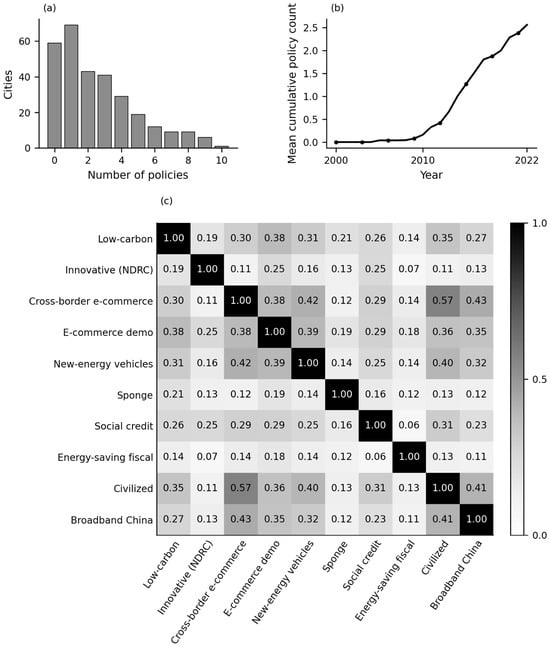
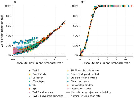
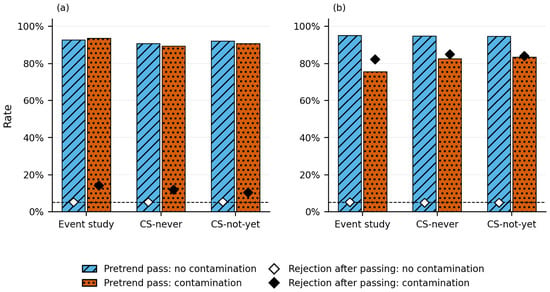
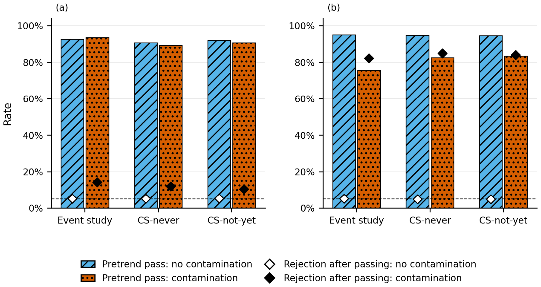

Disclaimer/Publisher’s Note: The statements, opinions and data contained in all publications are solely those of the individual author(s) and contributor(s) and not of MDPI and/or the editor(s). MDPI and/or the editor(s) disclaim responsibility for any injury to people or property resulting from any ideas, methods, instructions or products referred to in the content. |
© 2026 by the authors. Licensee MDPI, Basel, Switzerland. This article is an open access article distributed under the terms and conditions of the Creative Commons Attribution (CC BY) license.