


Abstract
Integrating seasonal cold storage into seawater district cooling can extend the use of natural cold resources across seasons and change the annual cooling supply mix by compensating for temperature-dependent limitations of direct seawater cooling. In this study, an 8760 h simulation evaluates hybrid cooling scenarios using a measured annual cooling-load profile from an operating district cooling branch supplying chilled water, totaling approximately 171 GWh. The system prioritizes direct seawater cooling, followed by discharge from a prescribed initial cold-energy inventory and turbo-chiller backup. Under the same intake conditions, approximately 42 GWh of initial storage reduces the chiller’s annual cooling share from 22.9% to 2.2%. For CS_0.198, with approximately 33.8 GWh of initial storage, a +2 °C source-temperature shift advances the 10% storage discharge cutoff from about day 274 to day 196. Increasing the prescribed daily heat-loss coefficient from 0.03% to 0.15% advances it to about day 239. Hourly pumping profiles and annual electricity comparisons show why this reduction in refrigeration duty does not ensure a comparable electricity reduction. For an annual electricity ratio R ≤ 1.5 relative to the constant-temperature benchmark, the selected storage capacity falls from 42.1 to 16.5 GWh as the intake diameter increases from 1.25 to 1.40 m. These results support joint assessment of storage availability, intake pumping and storage capacity in the preliminary design of hybrid seawater district cooling systems.
1. Introduction
Global warming is increasing cooling demand and the challenge of meeting it without increasing carbon emissions. Miranda et al. [1] projected higher cooling degree days between 1.5 and 2.0 °C of warming, including substantial relative increases in historically cooler regions. Van Ruijven et al. [2] showed that climate change can amplify energy demand growth beyond socioeconomic effects, drawing on relationships between temperature, income and consumption. Khosla et al. [3] linked these pressures to sustainable cooling provision. Together, these studies highlight the need to accommodate growing cooling demand while managing electricity requirements and emissions.
District cooling provides shared infrastructure for integrating alternative cooling resources. Caputo et al. [4] linked the flexibility of district thermal systems to source diversity and effective management, with benefits dependent on local operating and supply conditions. Østergaard et al. [5] traced the transition from compression-based production toward natural cooling and integration with other energy sectors. These perspectives connect district cooling decarbonization with the coordinated use of lower-carbon sources and existing networks.
Conventional systems commonly use electrically driven centrifugal (turbo) chillers or heat-driven absorption chillers, whose emissions depend on the electricity mix and the origin of the driving heat. Gang et al. [6] connected district cooling performance with technology integration and system optimization. Eveloy and Ayou [7] reviewed renewable and waste-energy sources, natural cooling and storage, alongside distribution losses and control. Their findings support evaluating source substitution together with plant operation and network electricity use. Natural cooling can reduce refrigeration requirements, but its contribution depends on source temperature, availability and the energy needed to circulate water.
For coastal districts, seawater cooling depends on ocean conditions and intake design. Hunt et al. [8] assessed technical potential and costs in relation to source temperatures, bathymetry, intake length and utilization. Mokhtari and Arabkoohsar [9] optimized a Caspian Sea data-center system through component sizing and annual operational assessment, identifying an investment–pumping-power tradeoff. These studies connect geographical resource availability with engineering design: a favorable seawater temperature provides a cooling opportunity, while intake and heat-exchanger sizing determine the useful supply and associated electricity demand.
Seawater can also improve mechanical cooling. Schibuola and Tambani [10] reported lower electricity use and urban heat release from modeled seawater-cooled chillers than from air-cooled chillers. This improves heat rejection while retaining refrigeration; direct cooling requires sufficiently low source temperatures. This distinction matters when estimating the share of compressor-free cooling. Hunt et al. [11] proposed pressurized-ammonia distribution to extend seawater cooling services. These complementary approaches show that intake, conversion and distribution arrangements jointly determine system performance and must be considered within consistent energy boundaries.
Direct seawater cooling nevertheless remains temperature-dependent. A shallow or nearshore intake can shorten offshore infrastructure while increasing exposure to seasonal variability. Auxiliary refrigeration covers the shortfall when source temperatures become unsuitable. Higher flow can improve heat transfer but increases hydraulic losses [8,9]. Seasonal cold storage offers a complementary response by retaining winter cold for later use. This also changes the timing of auxiliary refrigeration. Its value depends on whether useful stored cooling remains available during periods of insufficient direct seawater supply, making storage duration as relevant as initial capacity.
Storage research links material properties with usable cooling delivery. Alva et al. [12] reviewed storage technologies and operating requirements, while Oró et al. [13] examined cold-storage phase-change materials and heat-transfer enhancement. Their reviews distinguish energy capacity from cooling power, emphasizing that sufficient heat-transfer capability is required to deliver stored energy at the necessary rate. Skogsberg [14] reported that stored snow supplied approximately 93% of the first summer’s cooling demand at Sundsvall Regional Hospital. This demonstrates seasonal use of winter cold, although its applicability depends on climate, storage configuration and demand.
Operational and distribution studies show how storage interacts with cooling supply. Tang et al. [15] used load prediction and model predictive control to coordinate ice storage and chillers under time-of-use tariffs while examining sensitivity to forecast uncertainty. Hunt et al. [16] integrated seawater cooling with transported thermal storage to reach users beyond fixed networks. These studies address when stored cooling is dispatched and where it is delivered, emphasizing that storage performance depends on integration with the supply system.
For seasonal applications, Sreenath et al. [17] assessed site suitability and photovoltaic supply for snow-storage-assisted district cooling. Yan et al. [18] optimized combined seasonal ice and chilled-water storage, including heat-pipe dimensions, tank configuration and volume, and chiller capacity. Li et al. [19] modeled air-cooled seasonal storage and examined operating and structural parameters, including flow conditions. Together, these studies connect resource collection, equipment sizing and auxiliary cooling, showing that effective seasonal operation requires coordinated design across the storage and supply subsystems.
Thermal losses further influence seasonal performance. Allan et al. [20] estimated heat-loss coefficients from monitored ice stores, providing an empirical basis for models of heat exchange between storage and its surroundings. Vivian et al. [21] showed how storage size and insulation affect charging and discharge duration, alongside economic and emissions constraints. These findings link physical storage behavior with annual operation. Accordingly, retained energy, useful discharge duration and subsequent auxiliary cooling are complementary indicators of storage performance.
Hybrid seawater cooling also requires consideration of source variability. Youn and Im [22] assessed direct cooling, turbo chilling and absorption cooling under constant and variable seawater temperatures. Their analysis links source conditions with annual cooling allocation and supports evaluating natural and auxiliary cooling together. Youn and Im also examined the effects of heat-exchanger NTU and turbo-chiller performance on annual operation; the present study retains the reference component formulations to focus on finite seasonal storage and intake sizing.
Collectively, these studies establish the roles of source conditions, storage design and operational control. However, the combined effects of finite seasonal storage, variable seawater temperature and intake hydraulics remain insufficiently characterized within a common annual operating framework. In particular, their findings do not directly quantify how storage losses and source warming affect useful discharge duration together with the intake and storage sizes needed to meet a specified electricity criterion. A larger natural cooling share alone cannot resolve these questions because pumping demand and storage availability impose separate constraints. This defines a knowledge gap in connecting hourly cooling allocation and storage availability with heat-exchanger temperature constraints and the pumping electricity associated with intake design.
To address this gap, this study conducts an 8760 h simulation using the measured annual cooling-load profile of an operating district cooling branch supplying chilled water, totaling approximately 171 GWh. Hybrid scenarios prioritize direct seawater cooling, seasonal-storage discharge and turbo-chiller backup. With a prescribed initial inventory, the analysis quantifies how source-temperature shifts and storage losses affect useful discharge duration. Heat-exchanger inlet and outlet temperatures identify periods requiring supplementary cooling. Hourly pumping profiles and annual electricity comparisons then show how intake diameter influences the electrical benefit of storage and the capacity required by a common electricity criterion. By connecting these thermal and hydraulic results under common load and dispatch assumptions, the study provides a quantitative basis for preliminary joint sizing of seasonal storage and seawater intakes.
2. System Configuration and Study Boundary
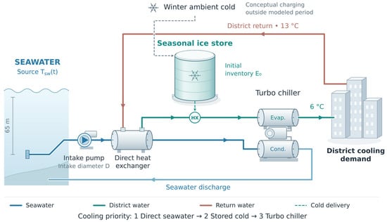
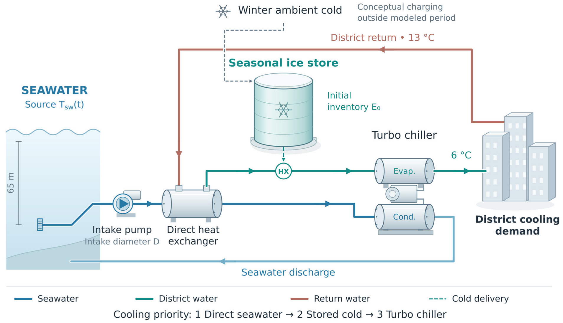
Figure 1 shows the hybrid supply arrangement: a seawater intake, direct heat exchanger, seasonal cold store, turbo chiller and district-water circuit. Direct heat exchange supplies cooling first. The store then covers residual demand while discharge remains available, and the chiller supplies the remaining load. Seawater leaving the direct heat exchanger also serves as the chiller condenser heat sink. This dispatch order allows seasonal storage to supplement the seawater cooling configuration without changing the priority assigned to direct cooling.
Figure 1.
Schematic of seawater district cooling with seasonal cold storage.
The seasonal store retains winter cold for subsequent cooling supply. Laboratory work on oscillating heat pipes supports the physical possibility of collecting sub-zero ambient cold [23] but does not establish charging rates or seasonal availability at district scale. The present analysis evaluates how an available winter cold inventory would affect subsequent annual cooling supply.
The store is assumed to be fully charged before the simulation begins. The calculation tracks its discharge and thermal losses over one year. The winter charging process is not explicitly modeled, and no recharging is allowed during the simulated period. This assumption isolates how the available seasonal cold inventory affects annual district cooling operation. Absorption chillers, investment appraisal and life-cycle carbon accounting are also outside the modeled scope. Table 1 summarizes the components and analysis boundary.
Table 1.
Model components and study scope.
Seasonal cold storage is represented by a prescribed initial inventory of usable cold energy, E0, which is assumed to be available before the modeled operating year. The storage medium is not specified in this system-level model. A possible hybrid charging pathway combining ambient winter cold and renewable-electricity-driven heat-pump charging is discussed in Section 5.3.
3. Methods and Input Conditions
3.1. Simulation Framework and Pumping Calculation
The analysis uses the hourly operating framework described by Liu et al. [24] and the seawater heat-exchanger and hydraulic models of Youn and Im [22]. Their component formulations are adopted here; the following sections specify the storage representation, input conditions and scenarios used in this study. Calculations use 8760 one-hour steps and do not resolve short-term equipment transients.
The shell-and-tube exchanger uses a reference design NTU of 2.0 and the seawater-flow control described in [22]. Flow is reduced from its allowable value when direct cooling exceeds demand. Each hour, direct seawater cooling is followed by storage discharge and turbo-chiller backup to meet the 6 °C supply target from a nominal 13 °C return. Storage availability does not independently trigger any further reduction in seawater flow under the adopted seawater-first dispatch. The storage inventory is then updated for delivered cooling and thermal losses.
Turbo-chiller electricity follows its assigned cooling duty and performance model [22,24]. The turbo-chiller performance model follows the seawater-assisted condenser-side formulation reported in [22], in which seawater is used as the condenser heat sink. The reference COP ranges from 5.6 to 9.52, with the operating COP determined according to the modeled condenser-side condition. Because intake pumping is a principal analysis variable, its electrical power is retained explicitly:
Here is water density, g is gravitational acceleration, V˙ is volumetric flow, Htot is total hydraulic head and ηp is pump efficiency. Head includes pipe friction calculated using [22] and applicable pressure and elevation terms; intake depth alone does not equal pumping head. With SI inputs, Equation (1) gives power in W, which is converted to kW for annual integration in Equation (5). Pipe friction follows the Hazen–Williams model reported by Youn and Im [22], using hourly seawater flow determined by the ε–NTU control. Because pipe friction is evaluated using the Hazen–Williams formulation, the Reynolds number and the Darcy friction factor are not explicit variables in the hydraulic calculation; manufacturer pump curves are not used as model inputs.
3.2. Seasonal-Storage Representation
Seasonal storage is represented by a lumped usable cold-energy inventory E, with 4 °C retained as the maximum usable cold-side temperature in the energy accounting. Each scenario begins at its specified initial inventory E0, corresponding to SOC = 1. With no charging term, the hourly balance is:
In Equations (2)–(4), energy is expressed in MWh, cooling and loss rates in MW, and Δt = 1 h. SOC is normalized by the initial inventory of each case, so identical SOC values do not imply identical available energy across differently sized stores.
Q˙SCS is useful cooling delivered from storage; Q˙loss is the loss rate of usable cold energy. Storage supplies demand remaining after direct seawater cooling while SOC > 0.10. Discharge stops at SOC ≤ 0.10, but thermal losses continue. The prescribed heat-loss coefficients are 0.03, 0.06, 0.10 and 0.15%/day, with 0.03%/day as the reference. Losses follow Q˙loss,t = λhEt, where λh is the hourly coefficient (h−1), λh = λd/24, and λd is the daily fractional coefficient (e.g., 0.03%/day = 0.0003 day−1). These inputs represent proportional losses, not measured insulation properties or cumulative annual losses. In Equation (4), Q˙load is cooling demand, Q˙HX is direct heat-exchanger cooling and Q˙TB is the residual turbo-chiller duty:
At each hourly step, seasonal storage supplies the cooling demand remaining after direct seawater cooling while SOC > 0.10. The storage inventory is updated for delivered cooling and the prescribed proportional thermal loss. Discharge stops when SOC reaches or falls below 0.10, whereas thermal losses continue. The cutoff time is defined as the first hourly step at which this condition is reached and is reported as elapsed simulation time; cases without a cutoff within 365 days are reported as not reached. The SOC cutoff represents cessation of storage discharge rather than complete physical depletion of the remaining cold inventory. At each hour, the turbo chiller supplies any residual demand remaining after direct seawater cooling and available storage discharge. The lumped model does not resolve storage geometry, internal temperature gradients, or detailed storage heat transfer and therefore does not verify the performance of a specific storage-system design. The resulting hourly storage-duty series defines the thermal-transfer requirement of the storage discharge interface. For representative cases, the maximum assigned duty was 27.4 MWth for CS_0.097 and 33.4 MWth for CS_0.198. These peak duties represent the minimum storage-side heat-exchanger thermal capacity required for the corresponding modeled operations. The model assumes that this duty can be delivered but does not prescribe the storage medium, circulation configuration, design temperature difference, UA, or heat-exchanger area; these equipment-design parameters should be determined for the selected storage technology and temperature approach.
3.3. Cooling Demand and Seawater Inputs
Cooling demand is based on measured data from an operating district cooling branch supplying chilled water [22], with an annual cooling delivery of approximately 171 GWh. The same 8760 h load profile is applied to the modeled coastal supply configuration in every scenario.
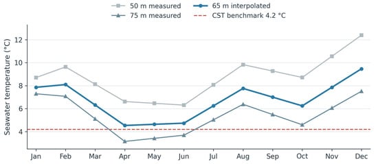
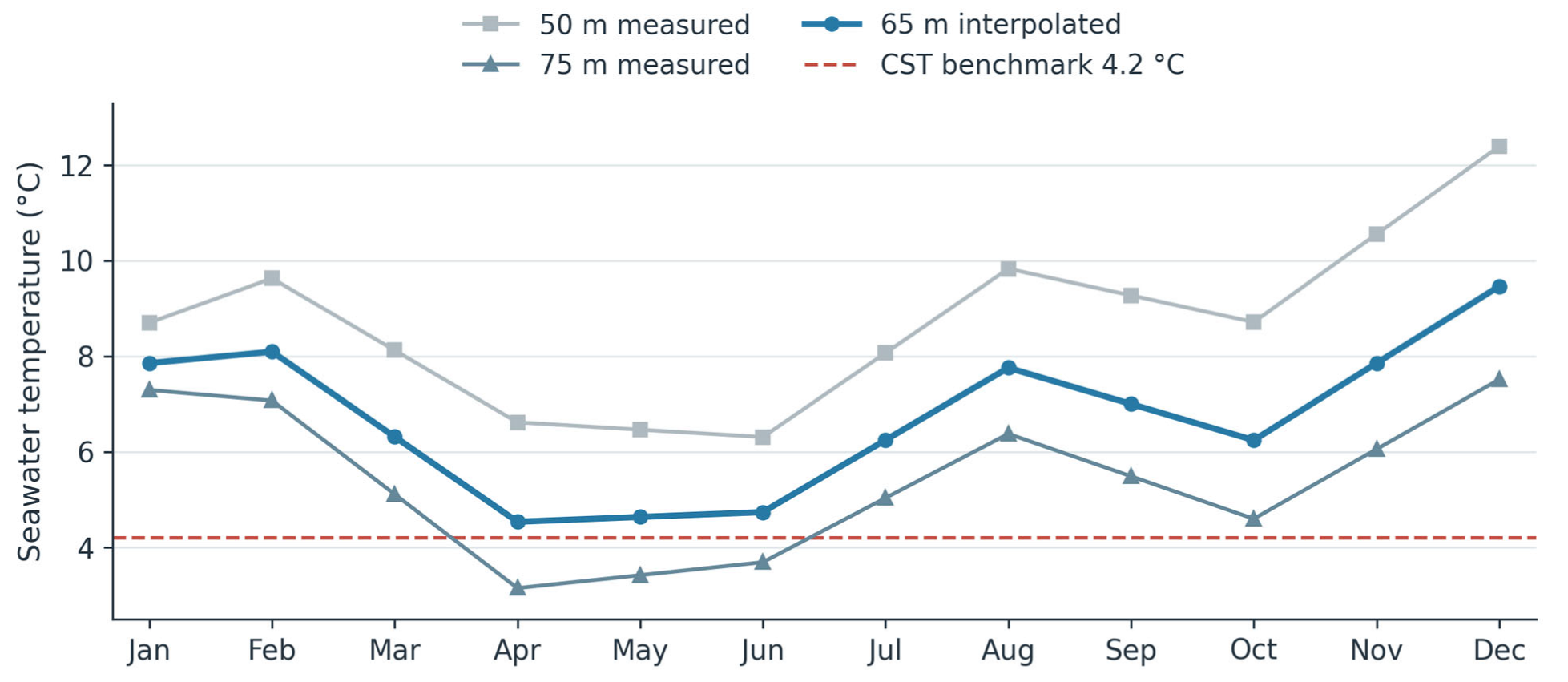
Monthly seawater observations from the Korea Oceanographic Data Center [25] define the variable-temperature source. The 65 m intake profile is interpolated in depth from observations at 50 and 75 m (Figure 2). Monthly values at 65 m range from approximately 4.5 to 9.5 °C, with an arithmetic mean of 6.73 °C. The constant-temperature benchmark is 4.2 °C throughout the year. Although cooling dispatch is calculated hourly, the environmental input remains based on monthly observations and does not represent measured hourly seawater variability.
Figure 2.
Monthly seawater temperatures at 50 and 75 m, interpolated to 65 m; dashed line: 4.2 °C CST benchmark.
CST and VST denote constant and variable seawater temperature. The CST intake is 6 km offshore at 200 m depth, whereas the VST intake is 2.5 km offshore at 65 m depth (Table 2). Their modeled intake lengths and load-side pipe lengths also differ. The CST–VST electricity ratio therefore compares complete configurations, not the isolated effect of source temperature. In contrast, VST cases with and without storage use the same intake geometry and temperature profile, allowing the effect of storage on cooling allocation to be assessed directly.
Table 2.
Reference intake and distribution conditions.
3.4. Scenario Design and Performance Indicators
Three linked comparisons use the same annual load and the dispatch order of direct seawater cooling, seasonal storage and turbo-chiller backup. Table 3 defines the reference and storage cases. REF_TB(CST) and REF_TB(VST) have no seasonal storage and use the intake configurations in Table 2. In NTU2.0_TB_CS_f, NTU2.0 denotes the reference heat-exchanger design NTU of 2.0, TB denotes turbo-chiller backup, and f is the initial cold-energy storage capacity normalized by the reference annual cooling demand of 171 GWh: f = E0/(171 GWh). The label does not specify the number of turbo-chiller units. Absorption chillers are excluded from all cases.
Table 3.
Reference and seasonal-storage scenarios and their initial cold-energy inventories.
Scenario suffixes give f rounded to three decimal places; Table 3 reports the corresponding storage inventories to one decimal place. Initial inventory differs from annual cooling delivered by storage because of heat losses and the 10% discharge cutoff.
First, the cases in Table 3 compare hourly cooling allocation, annual cooling shares and annual electricity at the reference seawater/load-side diameters of 1.0/0.8 m. The suffix _PD1.3 denotes a paired VST case in which only the seawater-intake diameter increases to 1.30 m; storage inventory and other operating assumptions are retained. This paired comparison precedes the intake-diameter sweep of 1.10–1.40 m. Second, source-temperature shifts of −1, +1 and +2 °C are applied at a 1.30 m intake diameter, preserving the seasonal pattern and cooling load. Third, CS_0.198, with approximately 33.8 GWh of initial storage, is used to evaluate temperature and heat-loss effects on discharge duration. This fixed-inventory series is distinct from the approximately 42 GWh CS_0.247 example.
The annual cooling share of each source is its integrated delivered cooling divided by the common annual cooling load. Annual electricity includes seawater pumping, district-water pumping and turbo chilling. Psw, Pload and PTB denote these three electrical powers, respectively. With power in kW and one-hour time steps, annual electricity in kWh is calculated as:
The electricity ratio R compares a VST configuration with storage against the CST benchmark. The prescribed criterion R ≤ 1.5 allows up to 50% more annual electricity than CST; only R < 1 indicates lower electricity use. This criterion is used to compare sizing requirements and is neither a cost threshold nor evidence of electricity parity.
Equation (5) represents electricity consumed during the modeled annual cooling-operation period and includes seawater-intake pumping, district-water pumping, and turbo-chiller electricity. Seasonal charging occurs before this operating period and is evaluated separately, as described later in Section 5.3, because the initial cold inventory is assumed to be established using winter ambient cold and renewable electricity available during the charging period. For the illustrative 42.2 GWh case, this charging pathway requires 8.44 GWhe under the stated assumptions. This charging requirement is reported separately and is not included in Equation (5) or R. Accordingly, R represents the annual operating-electricity ratio of the modeled district cooling system after the initial seasonal cold inventory has been established.
4. Results
4.1. Annual Cooling Contributions Across Scenarios
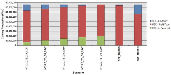
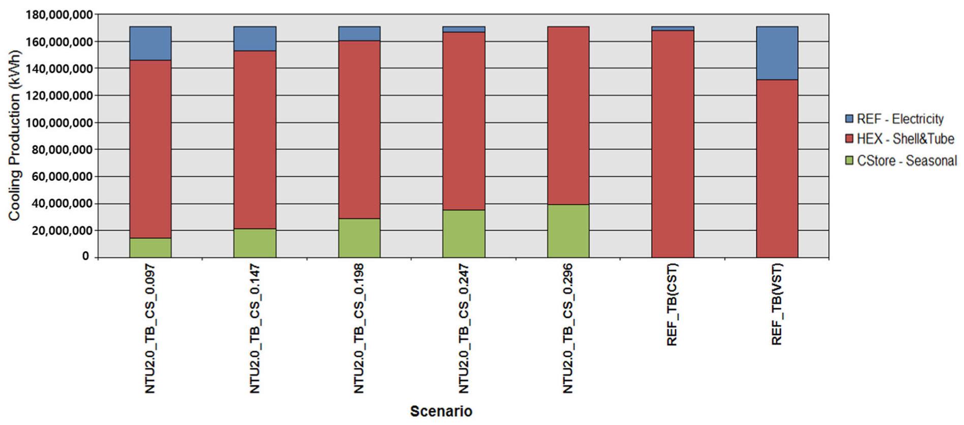
Figure 3 compares annual cooling production for the five storage inventories and the two no-storage references. All cases serve the same annual load. The CST reference requires only 1.8% of its annual cooling from turbo chillers, compared with 22.9% for VST without storage. Across the VST storage cases, the direct seawater contribution remains unchanged under seawater-first dispatch, while storage progressively replaces the residual chiller contribution. The CST and VST references use different intake configurations, so their comparison does not isolate seawater temperature alone.
Figure 3.
Annual cooling supplied by source for Table 3 scenarios at the 1.0 m intake. “REF–Electricity” denotes turbo-chiller cooling, not electricity consumption; absorption cooling is zero.
Under the same VST intake conditions, approximately 42 GWh of initial storage (CS_0.247) reduces the chiller’s annual cooling share from 22.9% to 2.2% (Figure 3). The reduction is 20.7 percentage points, equivalent to approximately 90.4% less chiller cooling duty. Seasonal storage thus covers most of the demand that direct seawater cooling cannot supply. This is a reduction in refrigeration duty; the corresponding change in total electricity depends on chiller performance and pumping.
Increasing the initial inventory further reduces reliance on auxiliary refrigeration. At CS_0.296, direct seawater cooling and storage meet the entire modeled annual load. This identifies a thermal supply outcome for the selected demand year and assumed initial charge, rather than an independently verified basis for removing backup equipment. The green storage contribution is useful cooling delivered during the year, rather than the initial cold-energy inventory listed in Table 3.
4.2. Hourly Cooling Allocation
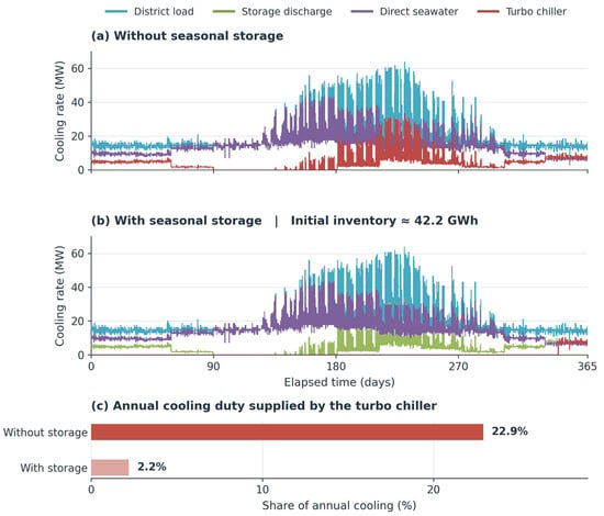
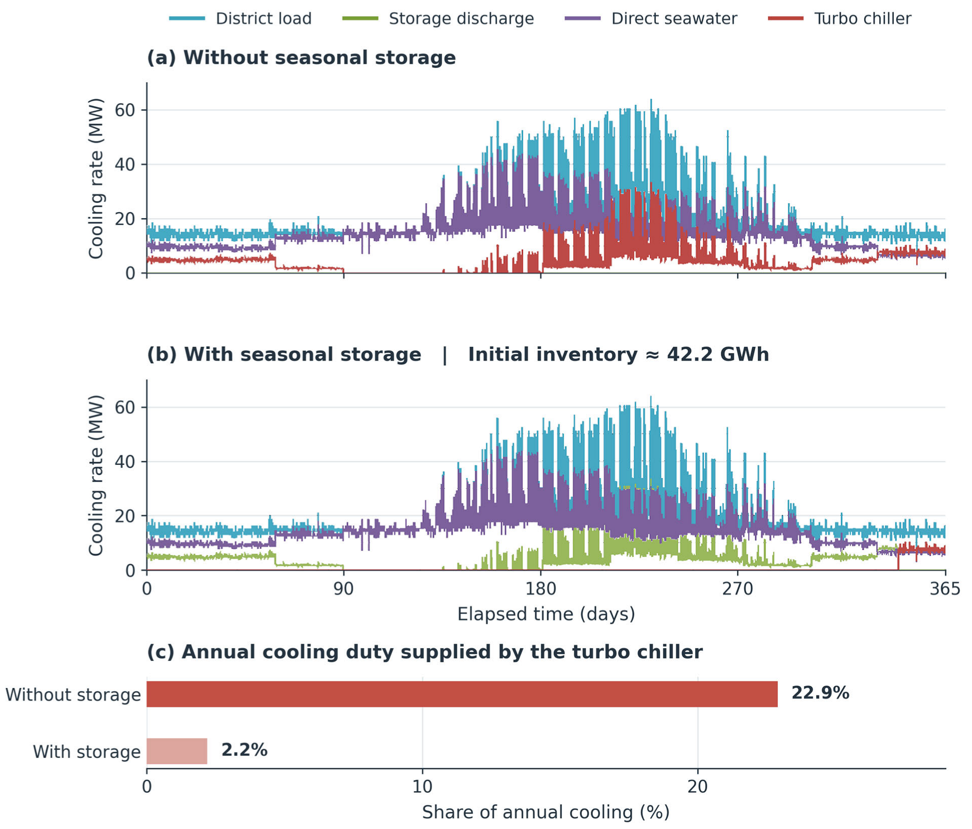
Figure 4 shows how the annual change arises from hourly dispatch. It compares VST operation without storage and with approximately 42.2 GWh of initial storage. The common intake geometry, seawater-temperature profile and cooling demand isolate the effect of adding a seasonal inventory.
Figure 4.
Hourly cooling allocation (a) without storage and (b) with CS_0.247 (42.2 GWh), and (c) annual turbo-chiller cooling share.
Without storage, the chiller supplies the recurring gap between direct seawater cooling and demand. With CS_0.247, storage covers much of that gap, including periods of high summer demand, before reaching the discharge cutoff. The benefit therefore depends on the timing of residual demand as well as its annual total: inventory consumed earlier in the year is unavailable for later periods of weak direct cooling.
Because dispatch prioritizes seawater, storage replaces downstream chiller duty without increasing the direct seawater contribution. Intake pumping consequently remains an important electrical load. These hourly allocations demonstrate when thermal substitution occurs, but neither annual cooling shares nor the absence of modeled chiller use establishes the required backup chiller capacity or peak electrical demand.
4.3. Effect of Initial Storage Capacity
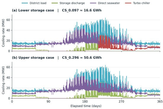
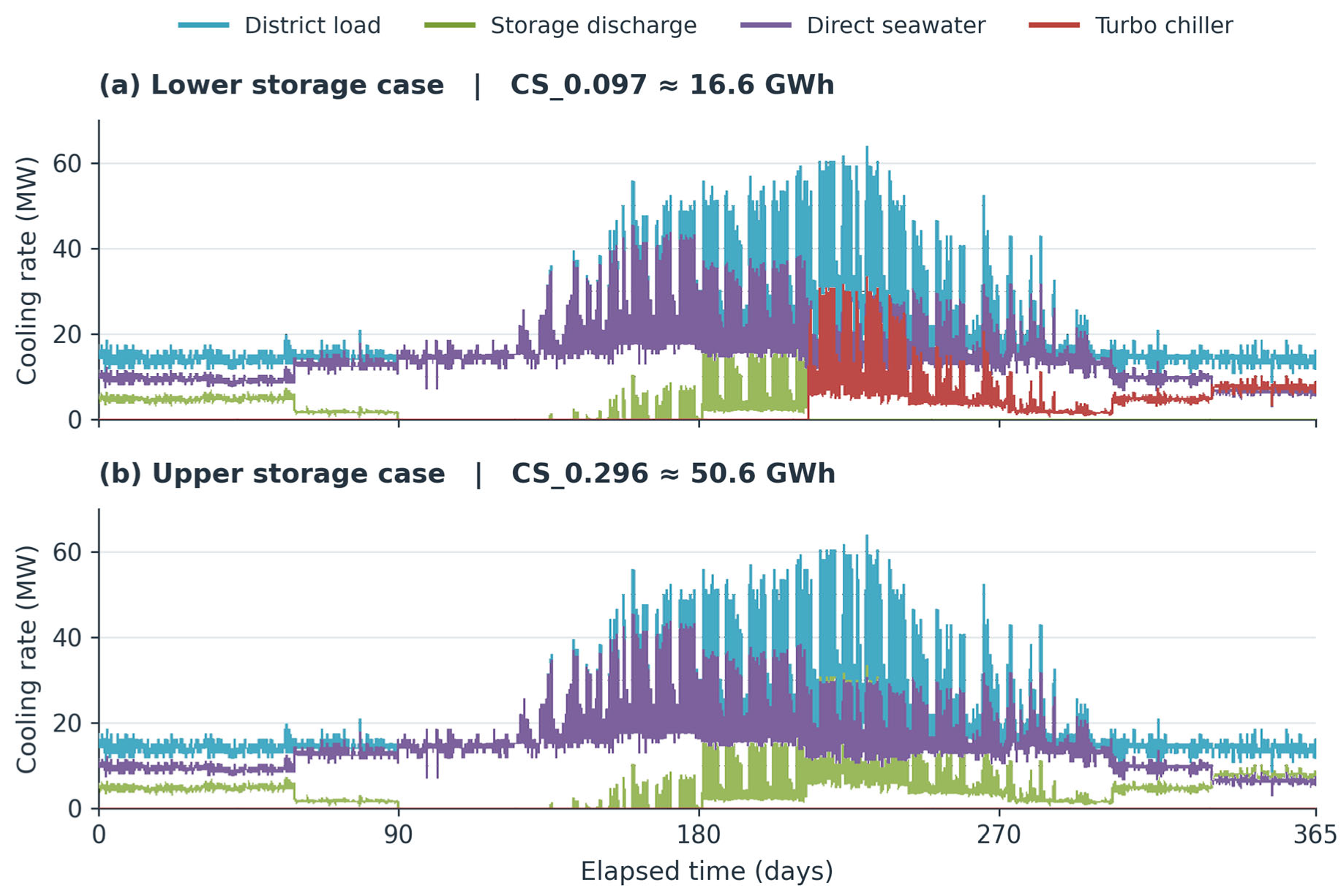
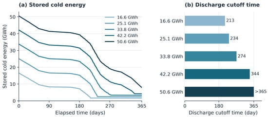
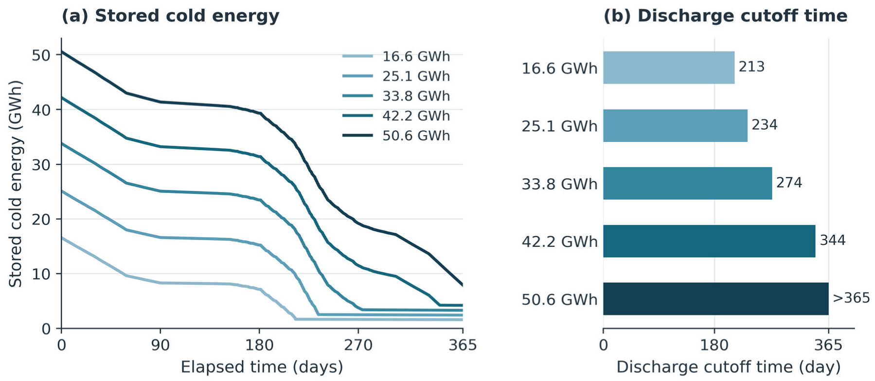
Figure 5 compares the lower and upper initial inventories. CS_0.097 requires auxiliary chilling earlier, whereas CS_0.296 covers residual demand throughout the modeled year. The trajectories in Figure 6 explain this difference by showing how each inventory is drawn down under the same demand and source conditions. Stored energy decreases through useful discharge and thermal losses (Figure 6). Steeper sections correspond to greater withdrawal to cover the gap between direct cooling and demand. Flatter sections indicate smaller withdrawals or loss-only decay. The curve shape therefore reflects the seasonal mismatch between cooling demand and available seawater cooling, as well as the initial inventory.
Figure 5.
Hourly cooling allocation for (a) CS_0.097 (16.6 GWh) and (b) CS_0.296 (50.6 GWh). CS_0.296 requires no turbo chilling under the modeled conditions.
Figure 6.
Storage-capacity sweep: (a) hourly stored energy and (b) 10% SOC discharge cutoff time. Values > 365 indicate no cutoff within the modeled year.
Smaller inventories reach the discharge cutoff earlier, after which the chiller must cover any residual demand. A larger inventory delays this transition. For CS_0.296, the cutoff is not reached within the modeled year, and a larger year-end inventory remains.
The positive inventory after discharge stops follows from the 10% control cutoff. Figure 5 and Figure 6 therefore support assessing storage capacity together with discharge duration. Remaining energy is not allocated to further cooling under this rule, although a different control threshold or storage design could change the usable inventory.
4.4. Heat-Exchanger Temperatures and Pumping Demand
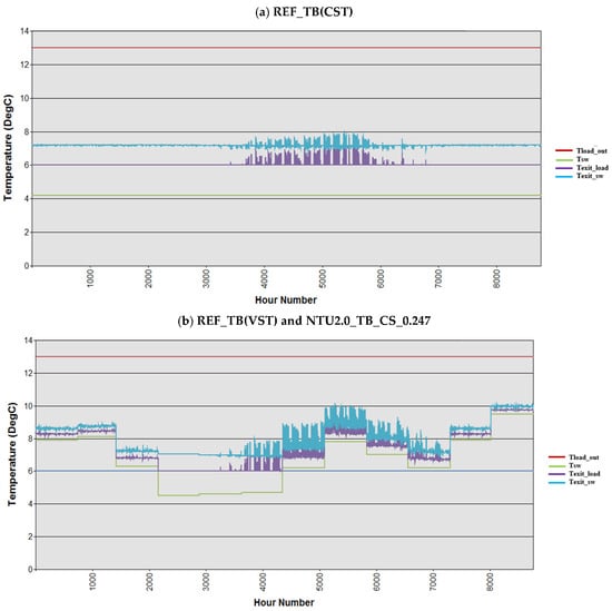
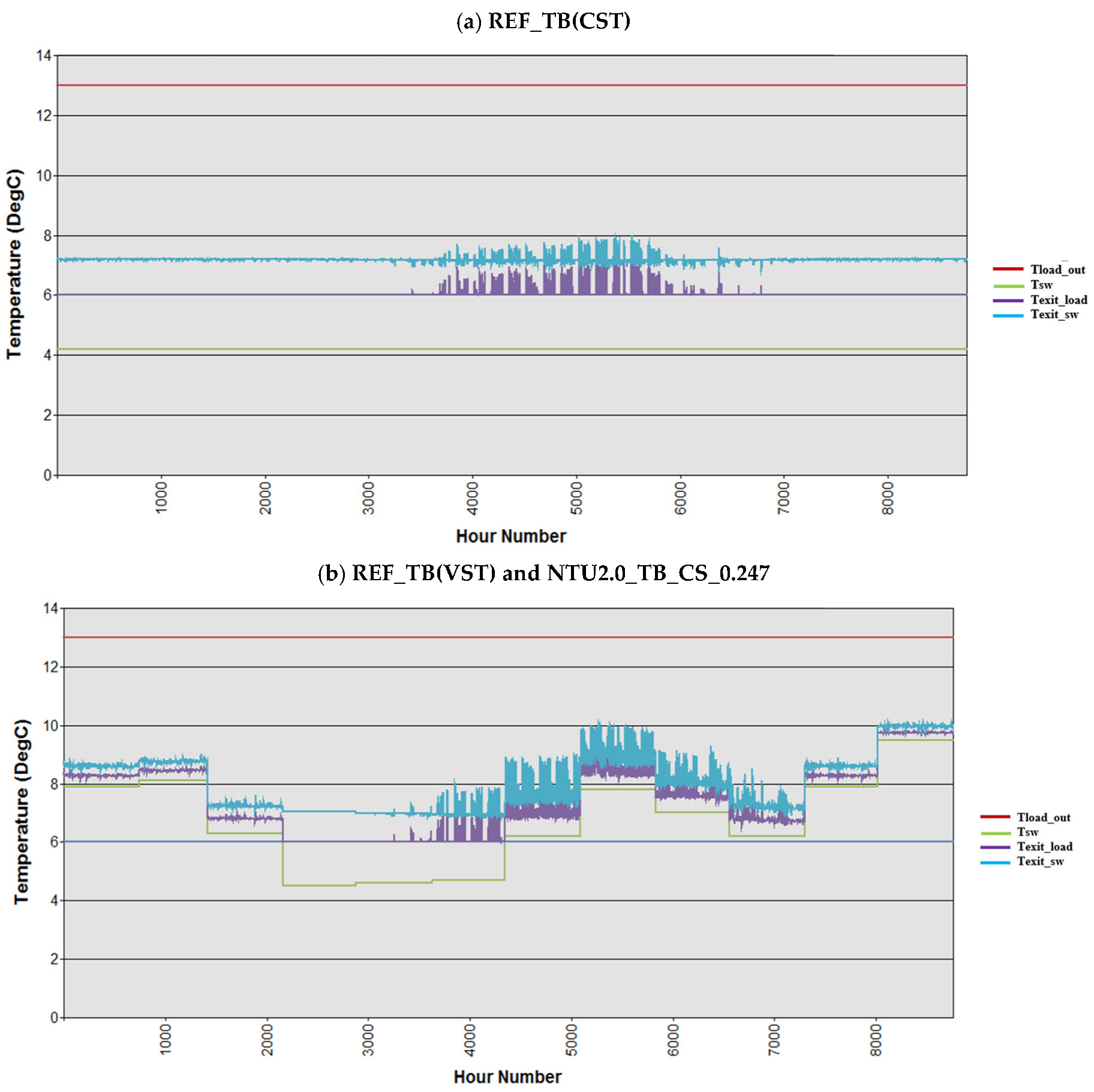
The direct heat-exchanger temperatures explain when supplementary cooling is required (Figure 7). With CST at 4.2 °C, the load-side outlet generally reaches the 6 °C supply target outside the high-load summer period. Its summer rise above 6 °C indicates that the exchanger cannot meet the full cooling duty at the modeled flow and heat-transfer conditions, despite the cold source. In VST operation, warmer seawater leaves a larger temperature gap over extended periods; the gap narrows during the cooler spring interval. The exchanger outlet is an intermediate temperature, whereas 6 °C remains the final district supply target after storage or chiller cooling.
Figure 7.
Hourly direct-HX temperatures for (a) CST and (b) VST with and without storage. Tsw/Texit_sw: seawater inlet/outlet; Texit_load: load-side HX outlet; Tload_in/Tload_out: 6/13 °C district-water reference temperatures.
The VST cases with and without CS_0.247 have the same direct-exchanger temperature profiles because storage operates downstream and seawater cooling retains priority. Seasonal storage therefore changes how the residual temperature gap is closed, without changing the displayed direct-exchanger response. When usable stored cooling is insufficient, turbo chilling covers the remaining duty. This temperature interpretation links the annual cooling shares in Figure 3 to the hourly allocation in Figure 4.
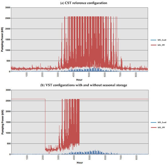
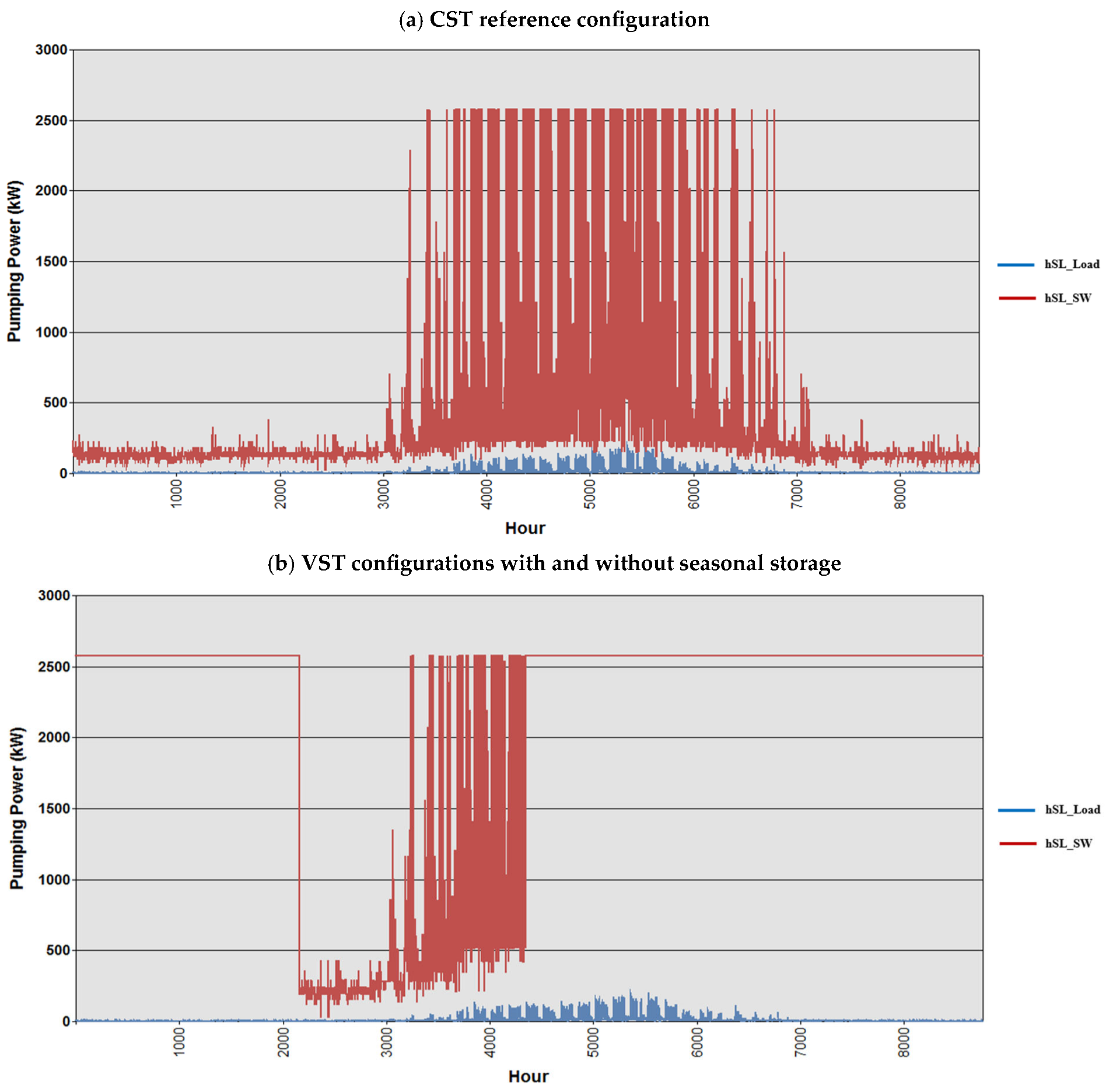
Figure 8 compares the annual hourly pumping-power profiles of the CST and VST configurations. Seawater-side pumping dominates load-side pumping in both cases. The much shorter load-side pipe reduces its total frictional head, whereas the intake must convey seawater over a kilometer-scale route (Table 2). The reference seawater pipe is also larger than the load-side pipe, at 1.0 versus 0.8 m, but diameter alone does not determine the relative power: flow rate and total head must be considered together.
Figure 8.
Hourly pumping power for (a) CST and (b) VST with and without storage (1.0 m seawater and 0.8 m load-side pipes). Blue: load-side; red: seawater-side pumping.
In the CST case, high intake-pumping demand is concentrated mainly in the high-load part of the year, and the plotted seawater-side power reaches approximately 2600 kW. In the VST cases, pumping remains close to this level over extended periods, with a marked reduction during the low-temperature spring interval. The warmer source requires greater seawater flow under the adopted heat-exchanger control even when district cooling demand is moderate. Thus, pumping demand reflects source temperature and flow control as well as cooling load. Since the CST and VST configurations also differ in intake length, these profiles compare complete configurations rather than isolating temperature alone.
Adding seasonal storage leaves the displayed VST pumping profile unchanged because direct seawater cooling retains dispatch priority. Storage supplies residual cooling downstream of the direct exchanger and reduces turbo-chiller duty without reducing the seawater flow selected by that control rule. This explains why a large reduction in annual chiller cooling share can coexist with a persistent intake-pumping burden. An alternative dispatch could reduce seawater-intake flow when stored cold is available, using additional storage discharge to compensate for any reduction in direct cooling. This could lower pumping electricity. At a fixed initial inventory and without recharging, the additional withdrawal could advance the SOC cutoff and increase subsequent chiller use if the remaining inventory becomes insufficient. Usable inventory that would otherwise remain above the cutoff at year end may offer opportunities for pumping savings without additional chiller operation. The annual modeled electricity benefit therefore depends on the timing of demand, seawater conditions, and available inventory. In the present study, this alternative dispatch strategy is discussed qualitatively, while its quantitative assessment, including the tradeoff between pumping-energy savings, storage depletion, and subsequent chiller operation, will be investigated in future work.
4.5. Annual Electricity Consumption and Intake Sizing
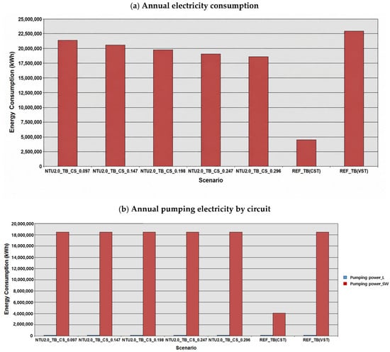
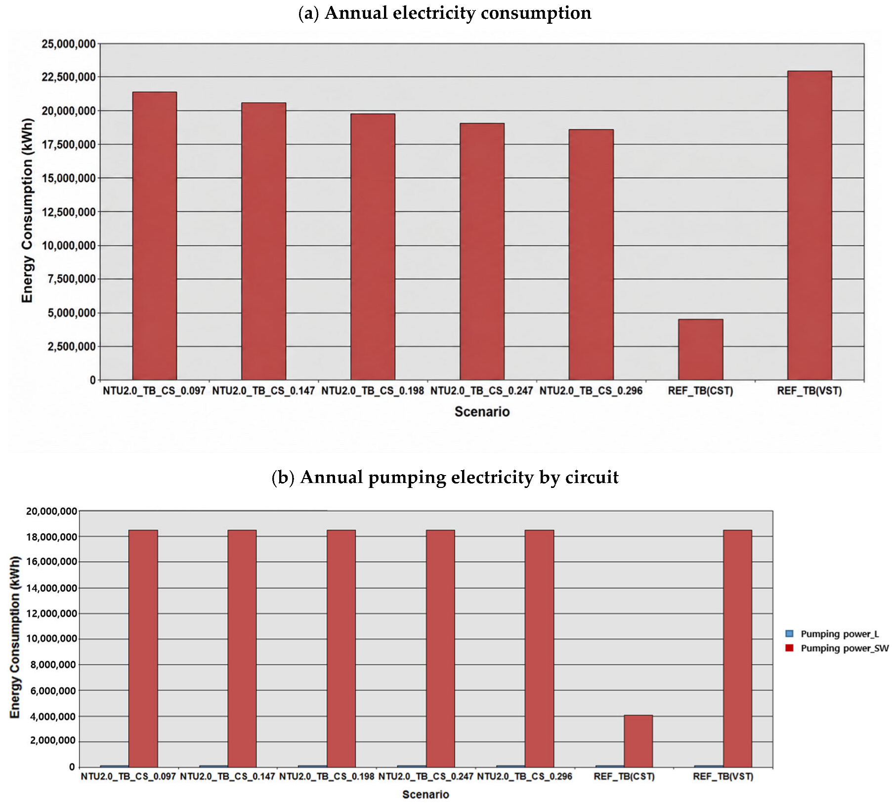
Figure 9 compares annual modeled operating electricity and the pumping contribution for the scenarios in Table 4. Increasing seasonal storage lowers total VST electricity by displacing turbo chilling, but seawater-pumping electricity remains nearly unchanged at the reference 1.0 m intake. Load-side pumping is much smaller. Consequently, even CS_0.296, which eliminates modeled turbo chilling, consumes approximately four times the annual electricity of the CST benchmark. The thermal substitution in Figure 3 therefore does not produce a proportional system-electricity reduction.
Figure 9.
Annual operating electricity at the 1.0 m seawater intake: (a) total electricity and (b) load-side and seawater-side pumping electricity. Panel (b) reports annual energy despite the original “Pumping power” legend.
Table 4.
Annual modeled operating electricity by scenario.
Table 4 reports annual modeled operating electricity in GWh under the Equation (5) boundary. Winter charging and storage-specific auxiliary electricity are excluded; the illustrative charging requirement is reported separately in Section 5.3.
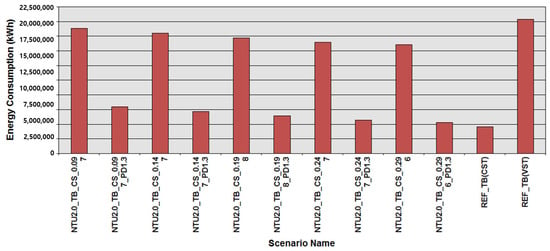
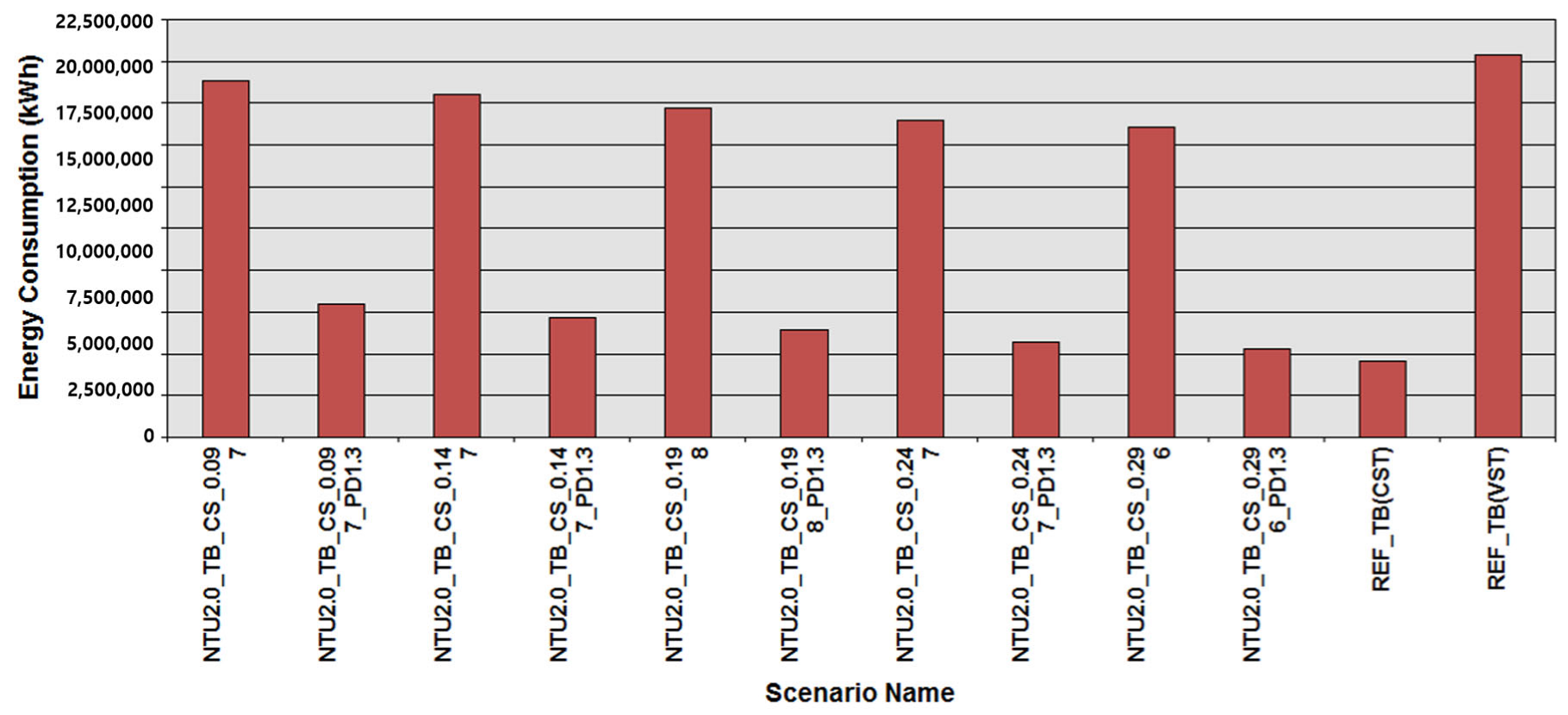
Figure 10 tests whether a larger intake can reduce this persistent pumping burden. Each _PD1.3 case is paired with the same storage scenario at the reference 1.0 m diameter. Increasing the seawater diameter to 1.30 m lowers annual electricity across the storage range, while additional storage continues to reduce residual chiller consumption. At the largest reference inventory, the 1.30 m case approaches R = 1.16, still approximately 16% above CST. Storage availability and intake sizing thus affect different parts of the electricity balance and need to be assessed together.
Figure 10.
Annual electricity for paired VST storage cases with 1.0 and 1.30 m seawater-intake diameters. _PD1.3 denotes 1.30 m; other operating assumptions are unchanged within each pair.
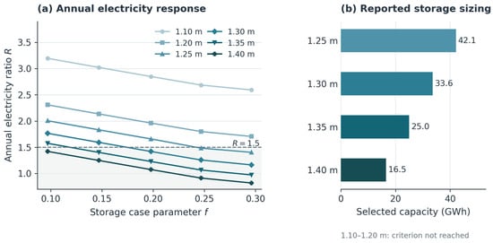
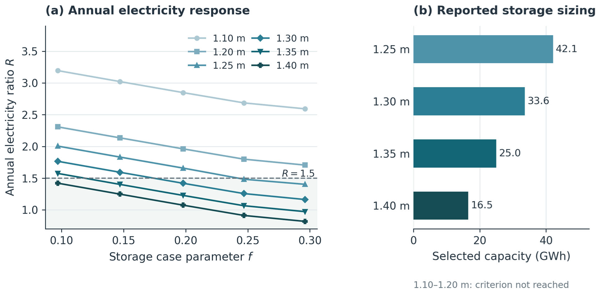
The wider diameter sweep in Figure 11 extends this comparison. At the largest reference storage setting, increasing the intake diameter from 1.10 to 1.40 m lowers R from approximately 2.59 to 0.82; at 1.30 m, R is approximately 1.16. Under the modeled boundary, the 1.40 m case uses about 18% less electricity than CST, whereas the 1.30 m case remains about 16% above it. Meeting R ≤ 1.5 therefore does not necessarily mean matching or improving on the benchmark. Along each curve, increasing storage lowers R by displacing chiller duty. At a given storage capacity, increasing the intake diameter lowers the pumping contribution, allowing the electricity criterion to be met with less storage.
Figure 11.
Intake-diameter effects on (a) annual electricity ratio R and (b) selected storage capacity. Dashed line: R = 1.5; panel (b) reports simulated sizing points. The shaded area in panel (a) indicates the region where R ≤ 1.5.
Neither the 1.10 nor 1.20 m intake meets R ≤ 1.5 within the investigated storage range. For the remaining diameters, Table 5 reports the discrete simulated storage capacity selected under the R ≤ 1.5 criterion. These values should not be interpreted as continuous optima; the exact threshold location depends on the resolution of the capacity sweep, and no interpolation between simulated points is applied.
Table 5.
Selected storage capacity by intake diameter under R ≤ 1.5.
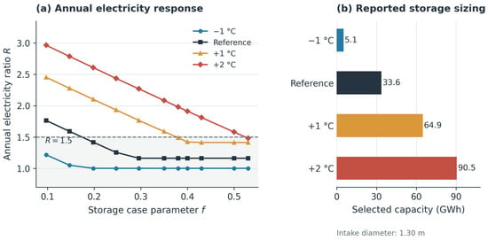
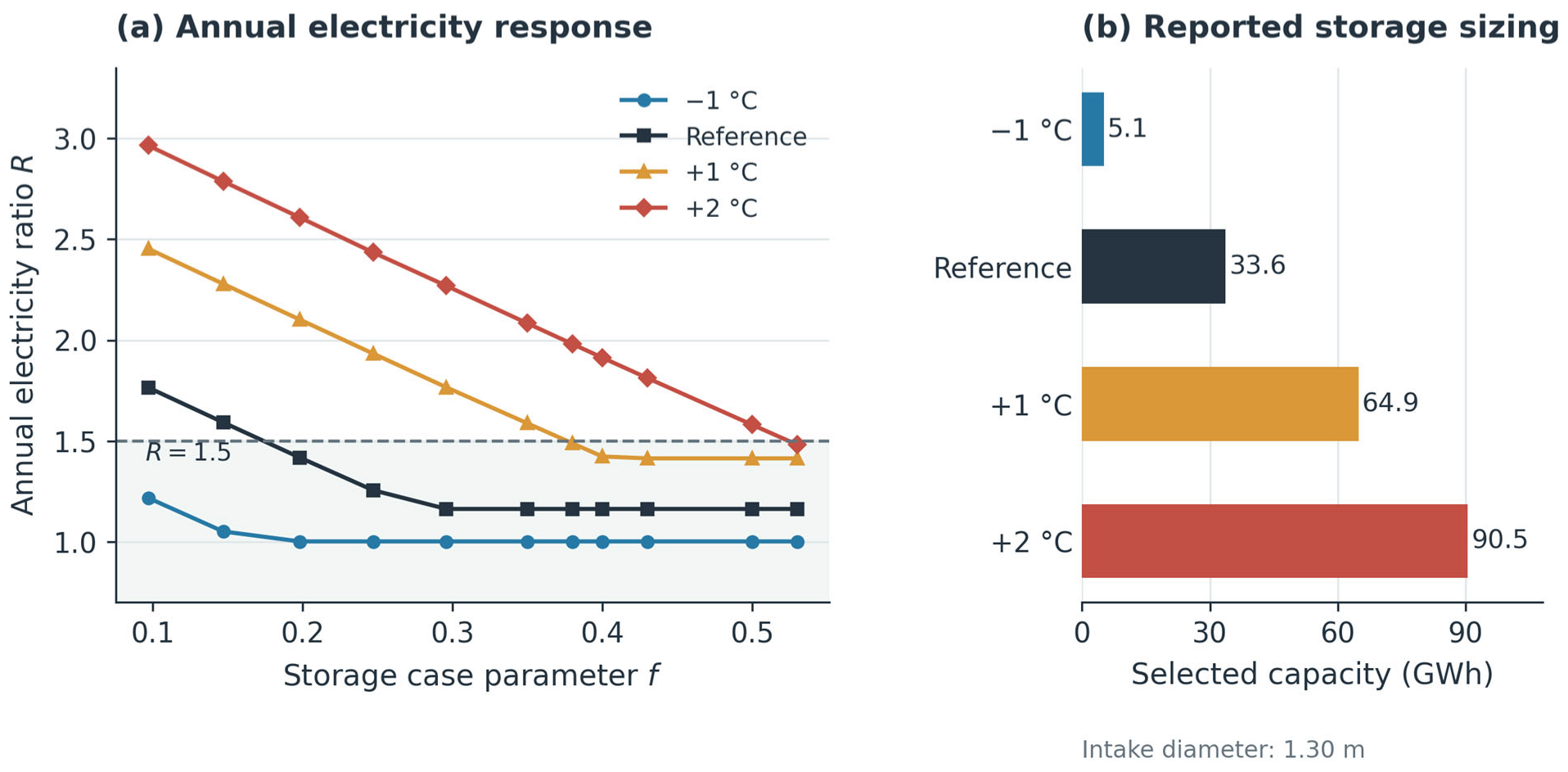
The complementary temperature sweep holds intake diameter fixed at 1.30 m. Warmer seawater increases R at a given storage capacity (Figure 12). A −1 °C shift reduces the residual cooling requirement, whereas +1 and +2 °C shifts increase it. Because the demand profile is held constant, these cases isolate supply-side temperature sensitivity. They do not predict future seawater conditions or include the additional cooling demand that a warmer climate could produce.
Figure 12.
Source-temperature effects at a 1.30 m intake: (a) annual electricity ratio R and (b) selected storage capacity. Dashed line: R = 1.5; the −1 °C sizing point lies below the storage range plotted in panel (a). The shaded area in panel (a) indicates the region where R ≤ 1.5.
Within the displayed range, the −1 °C, reference and +1 °C curves approach R values of approximately 1.00, 1.16 and 1.41, respectively. The +2 °C curve is still decreasing at the largest displayed setting. Once storage has displaced most residual chiller duty, additional inventory has little influence on the pumping required by seawater-first dispatch. These plateaus therefore describe the combined effect of source temperature and the fixed operating rule; a different dispatch strategy could change the electricity–storage relationship.
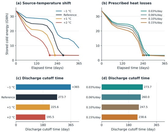
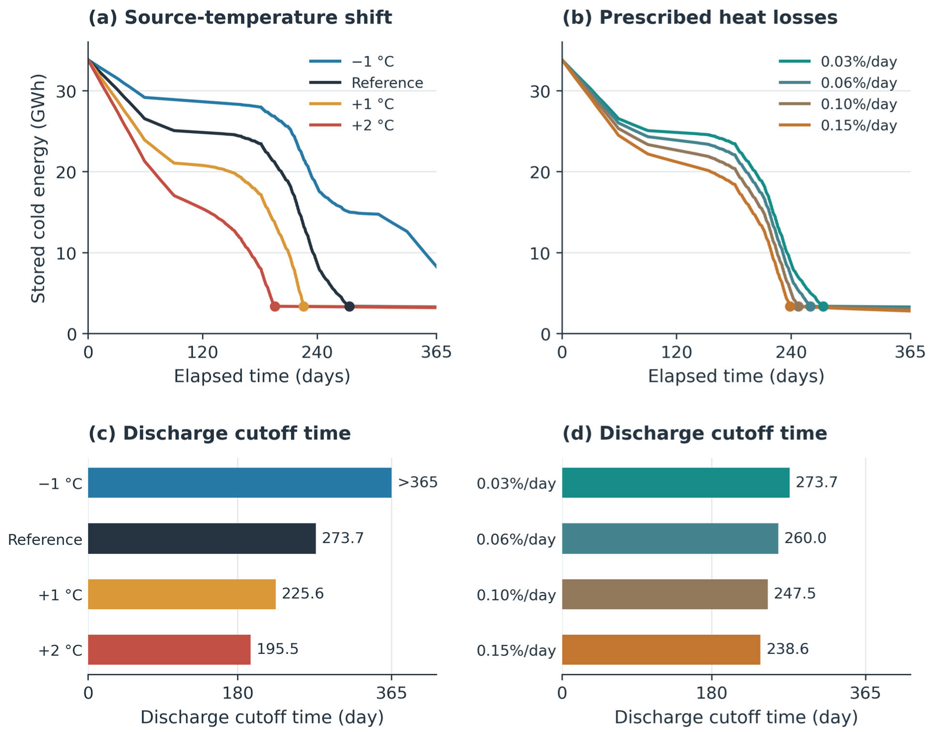
Because the −1 °C selected capacity lies below the range displayed in Figure 12a, its discrete sizing result is reported in Figure 12b and Table 6, and the plotted curve is not extrapolated. At a fixed 1.30 m intake diameter, the selected initial storage is 5.102 GWh at −1 °C, 33.632 GWh at the reference temperature and 90.481 GWh at +2 °C under R ≤ 1.5. With cooling demand fixed, warmer seawater reduces direct cooling, increases residual storage duty, and accelerates inventory drawdown. At the common 33.8 GWh inventory, the +2 °C shift advances the discharge cutoff from day 273.7 to day 195.5 (Table 7). The resulting capacity increase therefore reflects the coupled effects of source temperature, storage availability, chiller use, and pumping electricity.
Table 6.
Selected storage capacity by source-temperature shift at 1.30 m under R ≤ 1.5.
Table 7.
Discharge cutoff time and year-end inventory for CS_0.198.
4.6. Storage Availability Under Warming and Heat Loss
For CS_0.198, with approximately 33.8 GWh of initial storage, the reference case reaches the 10% discharge cutoff around day 274 (Figure 13). A +1 °C shift advances this transition to day 226, and +2 °C advances it to day 196, approximately 78 days earlier than the reference. At −1 °C, the cutoff is not reached within the year, and approximately 8.27 GWh remains. These results show how source temperature changes storage availability under the same initial capacity and discharge rule.
Figure 13.
CS_0.198 sensitivity: stored energy under (a) source-temperature shifts and (b) heat-loss coefficients, with corresponding 10% SOC cutoff times in (c,d). Values > 365 indicate no cutoff within the modeled year.
At the reference seawater temperature, increasing the prescribed daily heat-loss coefficient from 0.03% to 0.15% advances the cutoff from about day 274 to day 239, a reduction of approximately 35 days. Year-end inventory falls from 3.29 to 2.80 GWh. Earlier cutoff ends the storage contribution sooner, leaving any subsequent residual demand to the turbo chiller. Thermal decay continues below the 10% threshold, so positive remaining energy does not imply continued discharge under the adopted control.
The reference-temperature and 0.03%/day loss cases share one trajectory and are listed once. Cutoff times are elapsed days derived from hourly values under the SOC ≤ 0.10 rule. The influence of the discharge-control threshold was additionally evaluated for CS_0.198 under the +2 °C source-temperature shift using SOC cutoffs of 5%, 10%, 15%, 20%, and 25% (Table 8).
Table 8.
SOC cutoff sensitivity for CS_0.198 under the +2 °C source-temperature shift.
Increasing the SOC cutoff from 5% to 25% advanced discharge termination by approximately 542 h, or 22.6 days. A lower cutoff permits a larger fraction of the initial inventory to be used, whereas a higher cutoff preserves a larger operational reserve and terminates discharge earlier. These results confirm that the SOC threshold acts as an operational reserve criterion rather than a physical depletion limit. The absolute cutoff time remains dependent on the source-temperature condition. A cutoff not reached within 365 days does not establish uninterrupted discharge throughout the year; discharge also depends on residual cooling demand.
The electricity criterion and discharge cutoff time describe complementary design requirements. Warming increases demand on the store, whereas heat loss reduces the inventory available to meet it. A larger intake diameter can reduce pumping electricity, but a hydraulic improvement alone does not delay the storage cutoff if thermal dispatch is unchanged. Capacity selection should consequently consider the timing of residual demand in addition to annual electricity.
5. Discussion and Limitations
5.1. Cooling Allocation and Useful Storage Duration
The results address the knowledge gap by connecting annual cooling allocation with storage availability and intake electricity. Approximately 42 GWh of initial storage reduces the chiller’s cooling share from 22.9% to 2.2% under the same intake conditions (Figure 3). Under seawater-first dispatch, storage supplies residual demand rather than increasing direct seawater cooling. Its principal effect is therefore to extend compressor-free supply through periods when seawater alone is insufficient.
This thermal substitution does not imply a comparable reduction in total electricity because pumping remains necessary. Cooling share and annual electricity consequently describe different aspects of performance. Likewise, annual cooling shares cannot establish peak electrical demand or justify removing backup chillers.
For CS_0.198, +2 °C source warming and an increase in the prescribed daily heat-loss coefficient from 0.03% to 0.15% advance the discharge cutoff by approximately 78 and 35 days, respectively (Figure 13). Warming increases residual cooling demand, whereas losses reduce the available inventory. This supports evaluating capacity together with discharge duration, consistent with seasonal-storage studies [20,21]. The cutoff denotes cessation of storage discharge at the prescribed SOC threshold rather than complete depletion of the remaining cold inventory. The additional cutoff sensitivity analysis confirms that seasonal coverage depends not only on stored energy and source temperature but also on the selected operational reserve. The 10% cutoff used in the reference cases should therefore be interpreted as an operating assumption rather than a physical depletion limit.
5.2. Joint Intake Sizing and Storage Requirements
The temperature and electricity results explain why storage and intake sizing must be considered together. The direct-exchanger outlet identifies the residual cooling duty (Figure 7), while unchanged VST pumping under seawater-first dispatch explains why replacing that duty with storage does not remove the circulation burden (Figure 8 and Figure 9). The paired 1.0 and 1.30 m cases demonstrate the separate influence of intake diameter (Figure 10). Once storage largely displaces chiller duty, further electricity reductions require changes to intake or operating conditions. This supports the importance of pumping identified in seawater cooling optimization [9]. Under R ≤ 1.5, increasing diameter from 1.25 to 1.40 m reduces selected storage from 42.1 to 16.5 GWh (Table 5).
These values are conditional design relationships. R ≤ 1.5 permits up to 50% more electricity than the benchmark, and CST–VST comparisons include different intake configurations. Discrete capacity selections are not continuous optima. The matched VST diameter pairs isolate intake sizing more directly because source conditions, storage and dispatch are retained. Preliminary design should establish source temperature, route length, allowable flow and pipe resistance and then determine storage capacity and check useful discharge duration against residual cooling demand. A larger intake reduces friction but entails additional construction requirements. Pipe and storage costs are needed to assess whether the operating-electricity benefit justifies that investment.
5.3. Charging and Discharge Feasibility
A large seasonal inventory need not rely exclusively on passive ambient-cold collection. As an illustrative charging pathway, 20% of the initial inventory may be supplied by winter ambient cold and 80% by renewable-electricity-driven heat-pump charging. For a 42.2 GWh initial inventory, the heat pump would therefore provide 33.76 GWhth of cooling. Assuming 1000 equivalent full-load charging hours and a cooling COP of 4.0, this corresponds to approximately 33.8 MWth of heat-pump cooling capacity and 8.44 GWhe of charging electricity. If the associated photovoltaic system is also assumed to provide 1000 equivalent full-load generation hours over the charging period, an installed PV capacity of approximately 8.44 MWp would generate the required 8.44 GWhe. These estimates provide an order-of-magnitude basis for assessing the charging and renewable-power requirements, while subsequent system-design studies can further refine the coordination between PV generation and heat-pump charging.
5.4. Model Limitations and Decarbonization Implications
The measured cooling-load profile grounds demand in practice but does not validate the combined seawater–storage model. Monthly seawater inputs may miss short warm periods, and the temperature sweeps retain the same load rather than incorporating concurrent demand growth. Deterministic sweeps also do not propagate uncertainty in heat transfer, pump efficiency, roughness or fouling. The pumping calculations use fixed pipe-resistance and pump-performance assumptions; they do not test variable-speed pump selection or flow optimization coupled to storage dispatch. Storage duration is conditional on the prescribed loss coefficients and 10% cutoff. Measured charging and discharge data would be needed to validate physical storage performance and assess alternative operating limits.
Reduced refrigeration duty identifies a potential contribution to lower-carbon district cooling, but net emissions depend on the electricity mix, charging and storage auxiliaries, and infrastructure construction. Economic and life-cycle carbon assessments are therefore required before selecting an implementation. Within the stated boundary, the study fills the identified gap by relating cooling substitution and discharge timing to heat-exchanger temperatures, pumping electricity and required storage capacity under a common annual demand. These relationships support preliminary joint sizing and identify which configurations warrant detailed engineering and field validation.
6. Conclusions
This study assessed how seasonal cold storage can compensate for temperature-dependent limitations of direct seawater cooling in district cooling systems. An 8760 h simulation used the measured annual cooling-load profile of an operating district cooling branch supplying chilled water, totaling approximately 171 GWh. The analysis connected annual cooling allocation, useful storage duration, heat-exchanger temperatures, pumping electricity and required storage capacity.
Under the same intake conditions, approximately 42 GWh of initial storage reduced the chiller’s annual cooling share from 22.9% to 2.2%. Seasonal storage therefore extended compressor-free cooling by supplying demand that seawater alone could not meet. This reduction represents displaced chiller cooling duty; total electricity still depends on pumping and auxiliary operation.
For CS_0.198, with approximately 33.8 GWh of initial storage, a +2 °C source-temperature shift advanced the 10% discharge cutoff from about day 274 to day 196. Increasing the prescribed daily heat-loss coefficient from 0.03% to 0.15% advanced it to day 239. These results show why storage capacity, thermal losses and discharge control must be assessed together: residual energy below the cutoff remains in the store but is not used for cooling under the adopted operating rule.
The direct heat-exchanger outlet exceeded the 6 °C supply target during periods requiring supplementary cooling, while seasonal storage left its VST temperature response unchanged under the prescribed dispatch. Seawater-side pumping remained the dominant circulation load. Even when storage eliminated modeled turbo chilling, the 1.0 m intake retained annual electricity of approximately four times the CST benchmark; a 1.30 m intake reduced the ratio to approximately 1.16 at the largest reference inventory. Under R ≤ 1.5, increasing intake diameter from 1.25 to 1.40 m reduced selected storage capacity from 42.1 to 16.5 GWh. This criterion permits up to 50% more electricity than the benchmark. The results support joint evaluation of intake pumping, storage capacity and useful discharge duration.
The findings remain conditional on a prescribed initial inventory without intermediate recharging. Winter charging, discharge-power limits and integrated system performance require verification; economic and life-cycle carbon assessments are also needed. Within this scope, the study addresses the identified knowledge gap by quantifying how seasonal-storage availability and intake hydraulics jointly shape cooling allocation, electricity use and storage requirements. These relationships provide a basis for preliminary design of seawater district cooling with seasonal use of natural cold resources.
Author Contributions
Conceptualization, Y.H.I. and S.Y.; Methodology, Y.H.I. and S.Y.; Software, Y.J.Y. and Y.H.I.; Validation, Y.J.Y. and Y.H.I.; Formal analysis, Y.J.Y. and Y.H.I.; Investigation, Y.J.Y.; Resources, Y.J.Y.; Data curation, Y.J.Y.; Writing—original draft, Y.J.Y.; Writing—review & editing, S.Y.; Visualization, Y.H.I. and S.Y.; Supervision, S.Y.; Funding acquisition, S.Y. All authors have read and agreed to the published version of the manuscript.
Funding
This work was supported by the Rural Development Administration through the project “Development of small scale photovoltaic power generation and storage technology for agricultural application” (RS-2024-00399318).
Institutional Review Board Statement
Not applicable.
Informed Consent Statement
Not applicable.
Data Availability Statement
The data presented in this study are available on request from the corresponding author.
Conflicts of Interest
The authors declare no conflict of interest.
Abbreviations
The following abbreviations are used in this manuscript:
| Term | Definition |
| CST | Constant seawater temperature |
| VST | Variable seawater temperature |
| SDC | Seawater district cooling |
| SCS | Seasonal cold storage |
| SOC | State of charge |
| NTU | Number of transfer units |
| HX | Heat exchanger |
| TB | Turbo chiller |
| R | Annual electricity ratio relative to the CST benchmark |
References
- Miranda, N.D.; Lizana, J.; Sparrow, S.N.; Zachau-Walker, M.; Watson, P.A.G.; Wallom, D.C.H.; Khosla, R.; McCulloch, M. Change in cooling degree days with global mean temperature rise increasing from 1.5 °C to 2.0 °C. Nat. Sustain. 2023, 6, 1326–1330, Correction in Nat. Sustain. 2023, 6, 1716.. [Google Scholar] [CrossRef] [Scilit]
- van Ruijven, B.J.; De Cian, E.; Sue Wing, I. Amplification of future energy demand growth due to climate change. Nat. Commun. 2019, 10, 2762. [Google Scholar] [CrossRef] [Scilit] [PubMed]
- Khosla, R.; Miranda, N.D.; Trotter, P.A.; Mazzone, A.; Renaldi, R.; McElroy, C.; Cohen, F.; Jani, A.; Perera-Salazar, R.; McCulloch, M. Cooling for sustainable development. Nat. Sustain. 2021, 4, 201–208. [Google Scholar] [CrossRef] [Scilit]
- Caputo, P.; Ferla, G.; Belliardi, M.; Cereghetti, N. District thermal systems: State of the art and promising evolutive scenarios. A focus on Italy and Switzerland. Sustain. Cities Soc. 2021, 65, 102579. [Google Scholar] [CrossRef] [Scilit]
- Østergaard, P.A.; Werner, S.; Dyrelund, A.; Lund, H.; Arabkoohsar, A.; Sorknæs, P.; Gudmundsson, O.; Thorsen, J.E.; Mathiesen, B.V. The four generations of district cooling—A categorization of the development in district cooling from origin to future prospect. Energy 2022, 253, 124098. [Google Scholar] [CrossRef] [Scilit]
- Gang, W.; Wang, S.; Xiao, F.; Gao, D.-C. District cooling systems: Technology integration, system optimization, challenges and opportunities for applications. Renew. Sustain. Energy Rev. 2016, 53, 253–264. [Google Scholar] [CrossRef] [Scilit]
- Eveloy, V.; Ayou, D.S. Sustainable District Cooling Systems: Status, Challenges, and Future Opportunities, with Emphasis on Cooling-Dominated Regions. Energies 2019, 12, 235. [Google Scholar] [CrossRef] [Scilit]
- Hunt, J.D.; Byers, E.; Sánchez, A.S. Technical potential and cost estimates for seawater air conditioning. Energy 2019, 166, 979–988. [Google Scholar] [CrossRef] [Scilit]
- Mokhtari, R.; Arabkoohsar, A. Feasibility study and multi-objective optimization of seawater cooling systems for data centers: A case study of Caspian Sea. Sustain. Energy Technol. Assess. 2021, 47, 101528. [Google Scholar] [CrossRef] [Scilit]
- Schibuola, L.; Tambani, C. Performance assessment of seawater cooled chillers to mitigate urban heat island. Appl. Therm. Eng. 2020, 175, 115390. [Google Scholar] [CrossRef] [Scilit]
- Hunt, J.D.; Nascimento, A.; Zakeri, B.; Barbosa, P.S.F.; Costalonga, L. Seawater air-conditioning and ammonia district cooling: A solution for warm coastal regions. Energy 2022, 254, 124359. [Google Scholar] [CrossRef] [Scilit]
- Alva, G.; Lin, Y.; Fang, G. An overview of thermal energy storage systems. Energy 2018, 144, 341–378. [Google Scholar] [CrossRef] [Scilit]
- Oró, E.; de Gracia, A.; Castell, A.; Farid, M.M.; Cabeza, L.F. Review on phase change materials (PCMs) for cold thermal energy storage applications. Appl. Energy 2012, 99, 513–533. [Google Scholar] [CrossRef] [Scilit]
- Skogsberg, K. The Sundsvall Regional Hospital snow cooling plant—Results from the first year of operation. Cold Reg. Sci. Technol. 2002, 34, 135–142. [Google Scholar] [CrossRef] [Scilit]
- Tang, H.; Yu, J.; Geng, Y.; Liu, X.; Lin, B. Optimization of operational strategy for ice thermal energy storage in a district cooling system based on model predictive control. J. Energy Storage 2023, 62, 106872. [Google Scholar] [CrossRef] [Scilit]
- Hunt, J.D.; Issa, R.; Sanjivy, K.; Lucas, F.; Wada, Y. Integrating seawater air conditioning and mobilized thermal energy storage. J. Energy Storage 2025, 113, 115638. [Google Scholar] [CrossRef] [Scilit]
- Sreenath, S.; Kirs, T.; Kirs, K.; Volkova, A. Photovoltaic-powered seasonal snow storage-assisted district cooling system: Site suitability analysis and performance assessment. Energy 2024, 312, 133586. [Google Scholar] [CrossRef] [Scilit]
- Yan, C.; Shi, W.; Li, X.; Zhao, Y. Optimal design and application of a compound cold storage system combining seasonal ice storage and chilled water storage. Appl. Energy 2016, 171, 1–11. [Google Scholar] [CrossRef] [Scilit]
- Li, T.; Yu, H.; Qi, J.; Yuan, Y. Thermodynamic performance of air-cooled seasonal cold energy storage for space cooling: A case study. Renew. Energy 2024, 235, 121270. [Google Scholar] [CrossRef] [Scilit]
- Allan, J.; Croce, L.; Dott, R.; Georges, G.; Heer, P. Calculating the heat loss coefficients for performance modelling of seasonal ice thermal storage. J. Energy Storage 2022, 52, 104528. [Google Scholar] [CrossRef] [Scilit]
- Vivian, J.; Heer, P.; Fiorentini, M. Optimal sizing and operation of seasonal ice thermal storage systems. Energy Build. 2023, 300, 113633. [Google Scholar] [CrossRef] [Scilit]
- Youn, Y.J.; Im, Y.H. Assessment of the feasibility for hybrid seawater district cooling model under variable seawater temperature condition: Case study in South Korea. Renew. Energy 2023, 218, 119311. [Google Scholar] [CrossRef] [Scilit]
- Im, Y.H.; Lee, J.Y.; Ahn, T.I.; Youn, Y.J. Operational characteristics of oscillating heat pipe at sub-zero temperature for cold energy storage. Int. J. Heat Mass Transf. 2023, 201, 123598. [Google Scholar] [CrossRef] [Scilit]
- Liu, J.; Chung, D.-H.; Chung, M.; Im, Y.-H. Development of load models and operation simulator for a building complex with mixtures of multi-type engines and renewable devices. Energy Build. 2018, 158, 831–847. [Google Scholar] [CrossRef] [Scilit]
- National Institute of Fisheries Science, Korea Oceanographic Data Center. Oceanographic Observation Data. Available online: https://www.nifs.go.kr/kodc/ (accessed on 5 October 2026).

Disclaimer/Publisher’s Note: The statements, opinions and data contained in all publications are solely those of the individual author(s) and contributor(s) and not of MDPI and/or the editor(s). MDPI and/or the editor(s) disclaim responsibility for any injury to people or property resulting from any ideas, methods, instructions or products referred to in the content. |
© 2026 by the authors. Licensee MDPI, Basel, Switzerland. This article is an open access article distributed under the terms and conditions of the Creative Commons Attribution (CC BY) license.