


Abstract
Can artificial intelligence (AI) turn the agricultural, cultural and tourism endowments of less-developed regions into higher and more stable smallholder incomes? This study treats AI as an enabling condition that shapes how rural endowments are combined and monetised, not as a stand-alone treatment, and examines the coupling between the AI-enabled agriculture–culture–tourism (A–C–T) endowment system and smallholder income growth in Guangxi, Yunnan and Guizhou, China. Combining county administrative indicators for 328 county-level units (2022–2024) with a three-wave survey of 34,785 unique smallholder households (98,400 household-year observations; 30,842 households (94.0% of baseline) present in all three waves; income reference years 2022–2024), we construct entropy-weighted coupling coordination degrees and regress household income on a coordination measure rebuilt from officially published county statistics, not from the survey itself. The regional coupling coordination degree rose from 0.575 in 2022 to 0.746 in 2024; every county had exited the imbalance grades by 2024. A 0.1-point higher coordination index is associated with about 5.8 percent higher per-capita net income, an association robust to household fixed effects, province-by-year shocks and instrumental-variable estimation. Roughly one-third of the association is statistically accounted for by non-farm employment, tourism engagement and e-commerce participation, though these decompositions are associational rather than causal. The association is strongest where initial endowments are weakest but weaker for low-income than for better-off households—a capability divide. Income gains appear sustained across the three-year window; long-run durability remains untested.
1. Introduction
How smallholders can achieve income growth that endures remains one of the most consequential questions in development economics. Small-scale family farms, typically operating less than two hectares, constitute the overwhelming majority of the world’s 570 million farms and supply a large share of the food consumed in low- and middle-income countries [1], yet they remain structurally exposed to thin markets, weak asset positions and volatile returns [2]. In China, where more than 200 million smallholders still form the backbone of agricultural production, the question has acquired renewed urgency. With poverty eradication completed in 2020, the policy frontier has shifted from one-off poverty relief to durable income growth under a rural revitalization strategy that has moved the countryside to the centre of national development [3]. The No. 1 Central Documents of 2024 and 2025 each place the sustained increase in farmers’ income at the centre of this agenda, calling for the integrated development of agriculture, culture and tourism and for the accelerated application of new quality productive forces in the countryside [4,5]. These documents establish policy endorsement and direction; they are not, and we do not treat them as, evidence that the endorsed strategies work. Establishing whether they do is an empirical task, and it is the task of this study.
Nowhere is that task harder, or more revealing, than in the karst mountain corridor of Southwest China. Guangxi, Yunnan and Guizhou, home to the largest concentration of ethnic-minority populations in the country and to exceptionally rich agricultural, cultural and tourism endowments, combine the nation’s most severe historical poverty with its most distinctive rural assets [6,7]. Understanding what converts those assets into stable smallholder income there speaks directly to the broader puzzle of rural transformation.
A new candidate answer has emerged from the technology side. Artificial intelligence (AI), widely regarded as the defining general-purpose technology of the present era, reallocates tasks between labour and capital, compresses information frictions and reorganises production functions across sectors [8,9]. The macroeconomic literature has established that automation both displaces and reinstates labour, with the balance depending on the creation of new tasks and new markets [8]; the employment consequences are correspondingly heterogeneous [10]. In rural China, the diffusion of AI, embodied in smart-machinery, remote-sensing advisory systems, algorithmic marketing, intelligent recommendation of tourism products and digital-twin village governance, has been explicitly promoted as a carrier of new quality productive forces [11], and the Digital Village Development Strategy Outline has institutionalised the build-out of rural digital infrastructure since 2019 [12]. The agricultural literature documents rapid progress in smart farming, from big-data-driven input management to platform-based advisory services [13,14]. What remains poorly understood, however, is not whether AI can improve plot-level productivity but whether and how it accompanies a reconfiguration of the broader structure of rural factor endowments (the way agricultural resources, cultural resources and tourism resources are combined, valued and monetised), and whether that reconfiguration translates into income growth that smallholders can sustain rather than merely experience once.
This question has a natural systemic structure. The integration of agriculture, culture and tourism (hereafter A–C–T integration) is, at its core, a restructuring of factor endowments: land, labour, landscape, heritage and hospitality cease to be separable sectoral inputs and become jointly produced attributes of a territorial product. AI operates on this structure as an enabling condition and technological context (matching supply to demand, digitising cultural assets, and lowering the marginal cost of reaching distant consumers) rather than as a sector in its own right. Smallholder income growth, in turn, feeds back into the system: richer households invest in homestays, greenhouses and digital skills, deepening the very integration with which their income growth is associated. The relationship between the AI-enabled A–C–T factor endowment structure and smallholder income growth is, therefore, one of coupling—two interdependent systems co-evolving through reciprocal feedback—and its quality should be measured by the degree to which the two systems develop in a coordinated manner, not merely by the intensity with which they interact.
The present study examines this coupling at an unusually fine scale. We construct a two-system analytical framework in which System I is the AI-enabled A–C–T factor endowment structure and System II is smallholder income growth. Using a purpose-built county-year indicator system evaluated by the entropy weight method, we compute the coupling degree and coupling coordination degree of the two systems for all 328 county-level units of Guangxi (111), Yunnan (129) and Guizhou (88) over 2022–2024, and we link these measures to a stratified random survey of 34,785 unique smallholder households tracked over three annual waves, 30,842 of them present in all three (94.0% of the baseline sample)—98,400 household-year observations in which income refers to the calendar years 2022, 2023 and 2024. We keep two uses of the coordination measure strictly separate. The full coupling coordination degree (D), whose income subsystem embeds indicators aggregated from our own survey, serves only as a descriptive measure of regional coordination and is never used as a regressor. All income regressions instead employ a rebuilt measure (D′) in which the income subsystem is constructed entirely from officially published county statistics, independent of the household survey, so that the explanatory variable does not contain the outcome it is asked to explain. Two-way fixed-effects and instrumental-variable models relate household income to county-level D′; mechanism, heterogeneity and robustness analyses complete the design.
This study is organised around one main research question: to what extent, and through which channels, is the coordinated development of AI-enabled agriculture–culture–tourism endowments associated with smallholder income growth in an underdeveloped region? Three sub-questions decompose it. RQ1 (measurement). How did the coupling coordination between the AI-enabled A–C–T endowment system and the smallholder income system evolve across the 328 counties of Guangxi, Yunnan and Guizhou between 2022 and 2024, and which subsystem lagged? RQ2 (income association). Is higher county-level coupling coordination associated with higher smallholder per-capita net income, and does the association survive household fixed effects, province-by-year shocks and instrumental-variable estimation? RQ3 (channels and distribution). Through which household-level channels (labour reallocation, tourism engagement, e-commerce adoption) is the association statistically transmitted, and how is it distributed across provinces, ethnic groups and income strata?
The remainder of this paper proceeds as follows. Section 2 reviews the relevant literature and, in its closing subsection, states the gaps this study addresses and the contributions it makes. Section 3 presents the study area, data, the coupling-coordination methodology and the econometric strategy. Section 4 reports the results: the descriptive coupling characteristics first, then the econometric evidence. Section 5 discusses the findings against prior work, examines the institutional conditions that mediate them, and states the limitations of the design. Section 6 concludes with policy implications.
2. Literature Review
2.1. Artificial Intelligence and the Transformation of Agriculture
The scholarly assessment of AI in agriculture has moved quickly from engineering showcases to socioeconomic scrutiny. Early syntheses mapped the technological frontier (big data architectures, sensing, cloud platforms and decision support [13]) and set the agenda for social-science engagement with smart farming and Agriculture 4.0 [14]. Subsequent work complicated the optimism. Klerkx and Rose [15] warned that game-changing technologies reconfigure power and responsibility along the food system; Rose and Chilvers [16] argued for broadening responsible-innovation frameworks; and Fielke et al. [17] showed that digitalisation reorganises agricultural knowledge and advice networks, displacing some extension functions while creating others. Rotz et al. [18] and the FAO’s status report [19] documented how benefits are conditioned by connectivity, literacy and farm scale, foreshadowing a digital divide that mirrors, and may amplify, existing rural inequalities. Causal evidence on digital advice is more favourable but instructive: large-scale experiments show that well-designed digital advisory can shift practices and improve yields [20], though adoption frictions attenuate the gains [21]. Recent systematic reviews of AI-driven AgriTech [22], of the systemic risks of agricultural AI [23] and of its social and ethical footprint [24] converge on a common verdict: the technology is potent, but its rural-development value is mediated by institutions, capabilities and the structure of the local economy into which it is embedded. That verdict is what motivates the enabling-condition specification stated in the Introduction.
One conceptual distinction in the literature bears directly on how our results should be read, and it is too often blurred: smart agriculture, general rural digitalisation and direct AI applications are not the same thing. Smart agriculture denotes farm-level technologies in which sensing, data and algorithms inform production decisions—precision input management, drone-based crop protection, algorithmic agronomic advice [13,14,22]. General digitalisation is broader and older: connectivity (village broadband and 5G), digital marketplaces (e-commerce) and digital service channels (online booking) reorganise exchange and information flows without necessarily involving machine learning or algorithmic decision making [25,26]. Direct AI applications form the narrowest category: systems that perceive, predict, recommend or automate, such as yield-prediction models, recommender engines for tourism products and automated service delivery [23,24,27]. Our indicator system (Table 2 in Section 3) spans all three layers, and we classify each indicator accordingly: AI application scenarios (I1), smart-agriculture adoption insofar as the adopted packages are algorithm-based (A1) and smart-tourism services (T1) are AI-direct; village 5G/broadband coverage (I3), agricultural e-commerce sales (A2) and the online-booking share of tourist visits (T2) measure general digital infrastructure; and the remaining indicators—leisure-agriculture revenue (A3), the cultural-endowment measures (C1–C3), tourist reception (T3) and, in part, digital-skilled talent (I2)—record non-digital endowments and their human-capital context. What this study, therefore, measures is AI-conditioned endowment coordination. It does not isolate the contribution of artificial intelligence from that of the broader digitalisation alongside which AI diffuses, and we refrain from attributing the estimated associations to AI alone at any point below.
2.2. Digital Economy, E-Commerce and Smallholder Income
A second stream examines how the digital economy relates to farmers’ income. The foundational insight, that mobile connectivity reduces search costs and arbitrages price dispersion, dates to the early mobile-phone literature [25]. For China, the evidence has accumulated along several margins. Village-level experiments with e-commerce found limited average gains but notable heterogeneity [26]; household-survey studies using endogenous-switching designs consistently find positive income effects of e-commerce participation [28,29], as do analyses of Taobao villages [30], although critics caution that informality and platform fees erode the net benefit [31]. Recent work reports income gains associated with Taobao-village diffusion [32] and with e-commerce participation, with the largest counterfactual gains among low-income households [33]. At the macro level, the digital economy narrows some divides while widening others [34], exerts spatial spillovers on rural revitalization [35,36], interacts with digital finance in promoting common prosperity [37], and responds strongly to place-based e-commerce policies [38]; micro-econometric decompositions similarly identify information, employment and entrepreneurship channels [39]. These income dynamics unfold within a broader revolution in agri-food value chains that is reshaping the terms on which smallholders reach consumers [40]. First, digital access is not digital capability: effects depend on complementary household and local conditions. Second, the literature overwhelmingly measures the digital economy as an index or a policy dummy; it does not measure the structural configuration of the local endowments that digital tools act upon and, hence, cannot speak to coordination between the digital-endowment system and the income system.
2.3. Rural Tourism and Agriculture–Culture–Tourism Integration
Rural tourism research supplies the third stream. The concept has matured from a sectoral definition towards an integrated territorial understanding, in which agriculture, landscape, culture and community jointly constitute the product [41]. Agriculture and tourism demonstrably benefit one another when production, landscape and market functions are effectively linked [42], and the integrated-rural-tourism literature theorises integration as multidimensional: economic, social, cultural and institutional [43]. In China, rural tourism expanded explosively and was enrolled first into poverty alleviation and then into rural revitalization [44]; case studies show that village-level tourism can revitalise declining settlements when governance is inclusive [45]. The poverty-reduction literature is more cautious: tourism reduces poverty when participation is broad and institutions channel benefits locally [46,47]. Recent Chinese evidence ties agro-tourism integration and tourism-driven poverty reduction jointly to rural revitalization outcomes [48], evaluates tourism-village resilience from farmers’ perspectives in minority settlement areas [49], and identifies the mechanisms through which ecological farms integrate with rural tourism [50]. Meanwhile, automation and AI have entered tourism itself (service robots, algorithmic recommendation, intelligent interpretation), raising both productivity and questions about authenticity and employment [27]. What this stream has not produced is a quantitative account of how the endowment structure of A–C–T integration co-evolves with smallholder income at scale; integration is typically the explained variable, measured in a region, rather than an explanatory property of the system in which households are embedded.
2.4. Coupling Coordination as an Analytical Instrument
The coupling coordination degree model, imported from physics into regional science, has become the standard Chinese instrument for assessing whether two development systems evolve in step. Its modern form was consolidated in studies of urbanization–environment coordination [51] and tourism–environment coordination [52], and it has since been applied to rural public services and rural tourism in Southwestern China [7], to the digital economy and high-quality rural tourism [53], to the digital economy and rural revitalization [54], to rural tourism public services under digitalisation [55], to rural tourism and agricultural green development [56], to rural tourism and agricultural eco-efficiency [57], and, most recently, to the agricultural circular economy and rural tourism at the provincial scale [58]. Three lessons emerge from the literature. First, the coupling degree alone is uninformative when systems are closely linked (it saturates near unity), so the coordination degree, which incorporates development levels, must carry the analytical weight [58]. Second, nearly all applications use provincial or prefectural aggregates of a few dozen units, which limits statistical power and precludes micro-level inference. Third, no existing application couples an AI-conditioned endowment-structure system with a smallholder income system, and none validates the coordination measure against household-level outcomes.
Two interpretive cautions, underplayed in the literature, are stated in full in Section 3.2.3 and kept in view when interpreting the descriptive patterns of Section 4.1: entropy weights encode statistical information content rather than economic or welfare importance, and with the coupling degree C saturated near unity, the coordination degree tracks the matched development levels of the two systems rather than any deepening of their interaction.
2.5. Research Gaps and the Position of This Study
Read together, the three streams describe a clear frontier. AI scholarship shows that the technology’s rural-development value is mediated by local structure; the digital-economy literature finds income associations that are real but conditional on complementary capabilities; and the rural tourism and coupling-coordination literatures insist that integration be analysed systemically rather than sector by sector. What is missing is a framework that joins the three: one that applies the enabling-condition specification set out in the Introduction to the A–C–T factor endowment structure, measures the coordination of that structure with smallholder income growth, and probes the underlying channels with micro data.
Three specific gaps in the existing literature define the contribution of the present study. First, research on digital agriculture has concentrated on productivity and adoption at the farm or pilot scale, while research on A–C–T integration and rural tourism has remained largely macro-regional or case-based; the two streams rarely meet and almost never within a single micro-level inferential framework. Second, the smallholder income literature, though rich in evidence on e-commerce and digital finance, has generally treated digitalisation as an external treatment rather than as a property of the local endowment system, leaving the systemic coupling mechanism untested. Third, existing coupling-coordination studies rely overwhelmingly on provincial or municipal aggregates, typically with a few dozen spatial units, which precludes both household-level identification and credible statements about smallholders as opposed to regions. The present study addresses all three gaps within one design.
Table 1 positions this study against the five closest papers across five design dimensions: study unit, exposure, outcome, period and identification strategy.
Table 1.
Positioning of this study relative to the five closest papers: study unit, exposure, outcome, period and identification.
As the table makes clear, the closest studies either measure coordination at coarse spatial scale without an income outcome or estimate income effects of digitalisation without a systemic coordination measure. The present design combines the two: a large micro sample (Table 1) linked to a purpose-built county-level coordination measure rebuilt from officially published statistics. To our knowledge, this study is among the first to bring household-level identification to coupling-coordination analysis at this scale.
Against this frontier, this study makes three contributions. First, conceptually, it specifies a two-system coupling framework in which AI enters as an enabling condition acting on the endowment structure, not as a third coupled subsystem, clarifying a persistent ambiguity in applied coupling work. Second, methodologically, it scales coupling-coordination analysis to all 328 county-level units of three provinces, links the resulting measures to household panel data, and separates descriptive measurement (D) from explanatory use (D′) so that the outcome variable is never embedded in its own regressor. Third, empirically, it provides fixed-effects and instrumental-variable estimates of the association between coupling coordination and household income, decomposes that association into three household-level channels, and documents cross-county convergence alongside a capability gradient that policy must address.
Two limits of the design should be stated at the outset, because they discipline every claim that follows. The estimated relationships are associational; the instrumental-variable and falsification exercises support, but do not prove, a causal reading. The coordination measure, moreover, captures AI-conditioned digital-endowment development as a bundle: it cannot separate the effect of artificial intelligence proper from that of the general digital infrastructure with which it is deployed. We return to both limits in the discussion.
3. Materials and Methods
3.1. Study Area and Data Sources
The study area covers the complete set of 328 county-level administrative units in Guangxi Zhuang Autonomous Region (111), Yunnan Province (129) and Guizhou Province (88). In Guangxi, these belong to 14 prefecture-level cities: Nanning (12 county-level units), Liuzhou (10), Guilin (17), Wuzhou (7), Beihai (4), Fangchenggang (4), Qinzhou (4), Guigang (5), Yulin (7), Baise (12), Hezhou (5), Hechi (11), Laibin (6) and Chongzuo (7). In Yunnan, they belong to 16 prefecture-level units: Kunming (14), Qujing (9), Yuxi (9), Baoshan (5), Zhaotong (11), Lijiang (5), Pu’er (10), Lincang (8), Honghe Hani-Yi Autonomous Prefecture (13), Wenshan Zhuang-Miao Autonomous Prefecture (8), Xishuangbanna Dai Autonomous Prefecture (3), Chuxiong Yi Autonomous Prefecture (10), Dali Bai Autonomous Prefecture (12), Dehong Dai-Jingpo Autonomous Prefecture (5), Nujiang Lisu Autonomous Prefecture (4) and Diqing Tibetan Autonomous Prefecture (3). In Guizhou, they belong to 9 prefecture-level units: Guiyang (10), Liupanshui (4), Zunyi (14), Anshun (6), Bijie (8), Tongren (10), Qiandongnan Miao-Dong Autonomous Prefecture (16), Qiannan Buyi-Miao Autonomous Prefecture (12) and Qianxinan Buyi-Miao Autonomous Prefecture (8). The three provinces form a contiguous karst-mountain region that concentrates China’s richest ethnic-minority cultural resources, its most biodiverse agricultural systems and some of its fastest-growing rural tourism markets, while remaining among its lowest-income rural areas—an ideal setting for studying the conversion of endowments into household income.
Two data sources are integrated. The first is a county-year administrative panel for 2022–2024 covering the twelve System-I indicators listed in Table 2 and the three official income indicators of the rebuilt System II′. The panel was assembled from specified institutional sources, each responsible for the indicators in its statutory remit: the county statistics bureaus supplied the annual statistical communiqués and statistical yearbooks from which the rural income and output series are drawn; the agriculture and rural affairs bureaus supplied the smart-agriculture adoption returns and the agricultural e-commerce sales statistics; the culture and tourism bureaus supplied the intangible-heritage digitisation registry, the records of rural cultural venues, tourist reception statistics and platform booking reports; and the science and technology bureaus, together with county filings administered under the Ministry of Industry and Information Technology (MIIT), supplied the registry of AI application scenarios, the certified digital-talent counts and village-level 5G/broadband coverage. Where the same quantity appeared in two sources, the statistical communiqué figure was used and the alternative retained as a cross-check. Crucially, the three income indicators that enter the explanatory measure D′—the per-capita disposable income of rural residents, its official growth rate, and the inverse of its inter-annual volatility—come exclusively from these published county statistics and never from the authors’ household survey. Cross-bureau and across-year comparability was verified through common county-year keys, unit harmonisation to the stated denominators, and consistency checks of bureau returns against published prefectural totals.
Table 2.
Evaluation indicator system, definitions, sources, technology classification and entropy weights for the coupled systems, including the rebuilt income subsystem II′ used in the explanatory measure D′. The table reports definitions and denominators, source institutions, technology classes and supporting references for every indicator.
The second source is a stratified random household survey conducted by the authors in the first quarter of 2023, 2024 and 2025, with each wave recording income for the preceding calendar year; the income reference years are, therefore, 2022, 2023 and 2024, and all year labels in this study denote reference years, not fieldwork years. Within each county-level unit, 100 smallholder households, defined as family farms holding no more than 50 mu (3.33 hectares) of contracted cultivated land as recorded in the contractual land roster and deriving the majority of labour from family members, were randomly drawn from village rosters, yielding 32,800 households per wave and 98,400 household-year observations over the three waves. The selection criterion applies to contracted land, the quantity on which rosters and eligibility are based; operated land, which adds transferred-in parcels net of transfers out, can exceed the criterion, and it is operated land (maximal value 60 mu) that the descriptive statistics in Table 5 report. The two figures are, therefore, consistent: no sampled household held more than 50 mu of contracted land at selection. The survey collected household demographics, land and labour endowments, income by source, non-farm employment, participation in tourism and e-commerce, and perceptions of local AI-enabled services; the full questionnaire is described in Appendix A.
The design is a household panel with pre-specified, like-for-like replacement, not a series of independent cross-sections. At baseline (Q1 2023), 33,600 roster households were approached and 32,800 provided valid interviews, a response rate of 97.6 percent; the 800 losses combine screening failures, non-contacts, refusals and interviews that failed validation. In the second wave, 32,103 of the baseline households were re-interviewed (97.9 percent retention), and the 697 attritors (households that had moved, could not be contacted, or refused) were replaced from reserve rosters of pre-screened eligible households drawn at baseline in the same villages. In the third wave, 31,512 households from the wave-2 sample were retained (96.1 percent)—30,842 baseline-panel households and 670 wave-2 replacements—and the 1288 attritors were replaced from reserve rosters in the same manner, so that every wave file contains exactly 32,800 households, 100 per county. Wave-3 attrition (3.9 percent) was somewhat higher than wave-2 attrition (2.1 percent) and was similar in rate for continuing and replacement households. The balanced tracked core—households observed in all three waves—comprises 30,842 households (94.0% of the baseline sample). Table 3 reports the full flow of eligible, approached, responding, retained, replaced and excluded households by wave. Attrition is not only modest but approximately random with respect to the outcome: attritors and stayers do not differ on baseline per-capita net income (mean difference CNY 143, standard error CNY 201, t = 0.71), so replacement is unlikely to distort the income distribution of any wave. Estimation uses all 98,400 household-year observations; in fixed-effects specifications, each distinct household, including replacements, carries its own identifier. A county-by-wave sampling-flow table is provided as a Supplementary File.
Table 3.
Household sampling and panel flow by survey wave.
Table 4 sets out the calendar of fieldwork, recall periods, administrative reference years and index construction windows, making the alignment between the survey and the administrative panel explicit. Because the questionnaire records income of the preceding calendar year, the three waves map one for one onto the administrative years 2022–2024; the coupling indices for a given year are constructed from that year’s county indicators, and entropy weights are computed over the pooled 984 county-year observations to preserve intertemporal comparability.
Table 4.
Calendar of fieldwork, recall periods, administrative reference years and index construction windows.
Three procedures validate the survey data. First, household income aggregates were cross-checked against village rosters and against the officially published county means of rural per-capita income; the correlation between the survey-based county means and the official series is 0.87, high given the deliberate smallholder restriction of the sample frame. Second, five percent of interviewed households in each wave were randomly re-contacted by an independent verification team to confirm that the interview had taken place and that key items had been recorded accurately. Third, all questionnaires passed programmed logical checks (income components summing to totals, land transfers balancing, roster consistency) and were entered twice by different operators, with discrepancies reconciled against the paper instruments. Records failing these checks are among the exclusions reported in Table 3. The survey scales show high reliability and validity: the overall Cronbach’s α is 0.912, subscale α coefficients range from 0.83 to 0.90, the Kaiser–Meyer–Olkin measure is 0.934, Bartlett’s test of sphericity is significant at the 0.1 percent level, and confirmatory factor analysis yields standardised loadings between 0.62 and 0.87, composite reliabilities of 0.85–0.92 and average variance extracted of 0.54–0.68 (Table A1). These scales measure perceptions only. They are not used in any regression in this study, and the psychometric results speak to the quality of the perception module, not to the accuracy of the factual income reports or of the administrative data, which are secured by the validation procedures above.
Data integration proceeds at the county-year level: each household record is merged with the indicator vector of its own county and year, so that exposure to coordination varies across counties and over time but not across households within a county-year. All monetary values (survey income, revenue and sales indicators) are expressed in constant 2022 prices using the provincial rural consumer price indices before any transformation. Table 5 summarises the variable definitions and descriptive statistics for the integrated household-year sample.
Table 5.
Variable definitions and descriptive statistics (98,400 household-year observations unless noted).
The inferential population is defined by two scope decisions. First, the frame is the smallholder cultivator: landless non-cultivating rural households, and households whose income derives solely from tourism without any contracted farmland, fall outside it, as do larger commercial farms above the 50 mu contracted-land threshold. The results, therefore, describe the income coordination nexus for smallholder farm households, not for the entire rural population. Second, urban municipal districts enter the sample as county-level units on the same footing as counties and county-level cities, because they contain substantial cultivated land and smallholder populations in this region; a robustness check excludes the county-level units of the three provincial-capital prefectures (Table 12). Finally, equal sampling of 100 households per county implies equal county weights, not equal household selection probabilities across counties of different population sizes. The estimates are, therefore, county-representative: they describe the average smallholder in the average county of the region. Household-representative estimates require population weights, and a population-weighted re-estimation is reported in the robustness analysis (Table 12); the two agree closely.
Ethical clearance was granted by the Academic Committee of Guilin Tourism University, and verbal informed consent was obtained from all respondents prior to enumeration.
3.2. Analytical Framework and Methods
3.2.1. The Coupling Framework
Figure 1 presents the analytical framework. The coupling relationship investigated here runs between two systems: System I, the AI-enabled optimisation of the A–C–T factor endowment structure, and System II, the income growth of smallholders. AI enters the framework as the enabling layer specified in the Introduction and is not modelled as a third, parallel coupled system. The forward link runs from System I to System II: smarter endowment structures raise the marginal product of household labour and land and open new markets. The feedback link runs from System II to System I: higher and more stable household income finances investment in tourism facilities, digital skills and green production, deepening the optimisation of the endowment structure. Coupling coordination analysis measures how closely the two systems track one another through this reciprocal loop.
Figure 1.
Analytical framework in two panels. Panel (A): measurement architecture of the coupling between the AI-enabled A–C–T factor endowment structure (System I) and smallholder income growth (System II for the descriptive measure D; official-statistics System II′ for the explanatory measure D′), with AI drawn as a surrounding enabling band and the feedback loop between systems. Panel (B): hypothesised causal chain from D′ through the household-level mediators to income—hypothesised direction, tested as an association.
Figure 1 separates two things that are easily conflated. Panel A depicts the measurement architecture: System I with its four criterion layers (agricultural, cultural, tourism endowments and the AI enabling layer, the latter drawn as a band surrounding the endowment layers to mark its status as context rather than as a coupled subsystem), the two income subsystems—the survey-aggregated System II used in the descriptive measure D and the official-statistics System II′ used in the explanatory measure D′—and the feedback loop that justifies the coupling representation. Panel B depicts the hypothesised causal chain from county-level coordination (D′) through the three household-level mediators to income; it is explicitly labelled as a hypothesised direction that the econometrics tests as an association, not as an established fact. The descriptive use of D (Section 4.1) belongs to Panel A; the income regressions (Section 4.2) belong to Panel B.
3.2.2. Entropy Weight Method
To avoid the arbitrariness of subjective weighting, indicator weights are determined by the entropy weight method, which assigns larger weights to indicators carrying more information (greater dispersion) and is the standard objective weighting procedure in this area of the literature [7,56,61]. We index the two subsystems by distinct sets: j ∈ J1 = {A1, A2, A3, C1, C2, C3, T1, T2, T3, I1, I2, I3} for System I and k ∈ J2 = {S1, …, S5} for the survey-aggregated income subsystem, with J2′ = {S1′, S2′, S3′} for the official-statistics subsystem that replaces J2 in the explanatory measure. All indicators are first rendered dimensionless by range standardisation over the full sample of 984 county-year observations, so that intertemporal comparability is preserved:
where and are the original and standardised values of indicator j for observation i, n = 984 is the number of observations, is the share of observation i in indicator j, is the information entropy of indicator j, and its weight. , and denote the composite indices of System I, System II and System II′, obtained as the weighted sums of their respective standardised indicators. The resulting weights are reported in Table 2.
Equation (1) embodies two conventions that deserve explicit statement. First, the range is computed over the pooled panel; had any indicator exhibited zero range (an indicator constant across all county-years), it would have been dropped and assigned zero weight, since it carries no information. No indicator in either system triggered this rule. Second, the additive offset of 0.0001 keeps every standardised value strictly positive, so that the logarithms in Equation (3) are defined. The offset raises the normalized maximum to 1.0001, a bounded upward distortion of less than 0.01 percent; it is a standard convention of the entropy-weighting literature, and recomputing all indices without it leaves every county-year ranking and every substantive result below unchanged.
3.2.3. Coupling Coordination Degree Model
Following the consolidated practice of the coupling-coordination literature [7,51,58], the coupling degree C, the comprehensive coordination index T and the coupling coordination degree D of the two systems are computed as:
C ∈ [0,1] captures the intensity of interaction between the two systems; T is their weighted development level, with α = β = 0.5 reflecting the equal standing of the two systems, as is conventional [7,51]; and D = (C × T)^0.5 ∈ [0,1] captures both interaction intensity and matched development, discriminating between high-level coordination and low-level equilibrium. Because C saturates near unity when systems are closely linked, D carries the analytical weight in what follows [58]. We classify D into ten grades following established practice [7,52]: extreme imbalance [0, 0.1), high imbalance [0.1, 0.2), moderate imbalance [0.2, 0.3), low imbalance [0.3, 0.4), weak imbalance [0.4, 0.5), weak coordination [0.5, 0.6), low coordination [0.6, 0.7), moderate coordination [0.7, 0.8), high coordination [0.8, 0.9) and extreme coordination [0.9, 1.0].
Two coordination measures are carried through this study, and their uses are kept strictly separate. The full coupling coordination degree, D, couples System I with the original System II whose indicators are aggregated from our own household survey. Because those indicators embed household income (the outcome of the econometric analysis) together with its close transformations (growth, volatility, income-source shares), D contains the outcome in aggregated form. County aggregation reduces each household’s own contribution to the index but preserves both that contribution and the common county income component, so a regression of household income on D would partly relate income to itself. We, therefore, use D only as a descriptive measurement of regional coordination (Section 4.1, Table 6 and Table 7, Figure 2, Figure 3, Figure 4 and Figure 5) and never as a regressor. For explanation, we construct D′, which couples the same System I with the rebuilt System II′ of Table 2: the officially published per-capita disposable income of rural residents, its official growth rate and the inverse of its inter-annual volatility, all drawn from county statistical communiqués and none from the survey. D′ is computed exactly as in Equations (1)–(7) with U_2′ in place of U_2 and with recomputed income-subsystem weights; it excludes survey income, the income-source shares S4 and S5, and every proposed mediator. All regressions below employ D′.
Table 6.
Subsystem indices and coupling metrics by province, 2022–2024 (county means).
Table 7.
Distribution of the 328 county-level units across coupling-coordination grades, 2022–2024 (number of counties).
Figure 2.
Subsystem indices and coupling coordination degree by province, 2022–2024 (county means).
Figure 3.
Distribution dynamics of county-level coupling coordination, 2022–2024. Kernel density estimates use an Epanechnikov kernel with bandwidth 0.012 (Silverman’s rule).
Figure 4.
β-convergence of coupling coordination across the 328 county-level units.
Figure 5.
Grade composition of coupling coordination, 2022–2024: the composition of grades across counties; county-level transitions are reported in Table A2.
The relationship between the two income series nevertheless requires clarification. S1′–S3′ are officially published county-level indicators for rural residents, whereas the regression outcome is per-capita net income reported by sampled smallholder cultivators. The two series are related—sampled smallholders participate in the same rural economy, and their county means correlate with the official series at 0.87 (Section 3.1)—but they differ in population coverage, income definition and aggregation. No survey observation or survey aggregate enters D′, so there is no mechanical reuse of the dependent variable. Population overlap and shared county-level income conditions may nevertheless contribute to the estimated association; removing survey income from the index does not remove every source of endogeneity. We, therefore, retain an associational interpretation and report the System-I-only specification, which excludes all income indicators, as an additional check (Table 12).
The construction also disciplines interpretation. With C saturated near unity throughout the sample, temporal movements in either measure operate almost entirely through T: a rising D (or D′) signals that the two systems are developing together at matched and rising levels, not that the intensity of their interaction (already near its ceiling) has increased. The entropy weights, moreover, reflect the information content of indicators, not their economic or welfare importance, and the indices measure systemic co-movement rather than any social welfare function. We, therefore, read changes in coordination as changes in the matched development of the two systems, and we resist assigning them a broader economic meaning than the method supports.
3.2.4. Econometric Strategy
To estimate the association between coupling coordination and smallholder income, we estimate two-way fixed-effects models of the form:
where is the natural logarithm of per-capita net income of household i in county c in year t; is the county-year coupling coordination degree built from official statistics; is a vector of household controls (education, household size, labour force, cultivated land, ethnic-minority status, age of the household head and distance to the nearest rated scenic spot); and are household and year fixed effects; and is an idiosyncratic error. Standard errors are clustered at the county level throughout, following the practitioner guidance on cluster-robust inference [62,63]. Because D′ varies at the county-year level, identification comes from within-county variation over time, net of year shocks and, in the richest specifications, province-by-year shocks. All specifications share a common control set so that the county-effects, household-effects and instrumental-variable models are directly comparable: columns (1)–(3) net out year shocks, and columns (4)–(5) net out province-by-year shocks, exactly as reported in Table 8. Time-invariant controls are absorbed by household fixed effects and are reported only where they are identified (Table 8 and Table A3).
Table 8.
Baseline estimates: coupling coordination (D′) and smallholder per-capita net income.
After fixed effects, a causal reading still faces two threats: reverse causality from income to coordination, and measurement error in the constructed index. We address them with an instrumental variable, while being explicit about what the strategy can and cannot deliver. The instrument is the leave-one-out mean of D′ among the other counties of the same prefecture in the same year. Relevance is mechanical and strong: counties within a prefecture share planning programmes, infrastructure rollouts and market conditions, so neighbouring-county coordination predicts own-county coordination (first-stage F = 64.6). The exclusion restriction asserts that, conditional on own-county coordination, household effects and year effects, the coordination of other counties in the prefecture affects a household’s income only through its own county’s coordination. We regard this assumption as plausible but contestable: shared prefectural programmes (subsidised digital-village rollouts, prefecture-wide tourism promotion) could in principle reach households directly, violating exclusion. Three features of the design mitigate, without eliminating, the concern. The household fixed-effects specification with province-by-year effects absorbs all shocks common to a province in a year, of which prefectural programme waves are a subset insofar as they align with provincial cycles; for the preferred county-fixed-effects estimate, standard errors clustered at the level of the 39 prefectures and Conley spatial-HAC standard errors allowing dependence within 100 km leave its precision broadly intact (Table 12); and the IV estimate (0.579) is statistically indistinguishable from the preferred county-fixed-effects estimate (0.566), though it lies below the household-fixed-effects estimate (0.793). We do not read this proximity to the county-effects benchmark as proof of exogeneity—a Durbin–Wu–Hausman comparison against the household-effects estimate would reject it—but as evidence that the county-level association is not an artefact of within-household averaging. We, therefore, interpret the estimates as robust associations supported by causal evidence, not as definitive proof of causation. The first-stage and second-stage equations are:
where is the leave-one-out prefecture-year mean of D′, μ_i denotes household fixed effects, and λ_{p(c),t} denotes province-by-year effects for the province p(c) containing county c, matching the province-by-year specification reported in column (5) of Table 8. The instrument is constructed from the rebuilt D′, so the first stage never touches survey-aggregated income.
Mechanism analysis follows the causal-steps logic of Baron and Kenny [64] as disciplined for modern causal inference by Jiang [65]: each candidate mediator M (non-farm employment share, tourism engagement and e-commerce adoption) is first regressed on D′, and the income equation is then re-estimated with all mediators included:
In Equations (11) and (12), μ_c denotes county fixed effects: the mediation models are estimated under the preferred county-and-year-effects specification of Table 8. Because mediators and income are measured contemporaneously, Equations (11) and (12) decompose the association statistically; they do not identify causal mediation, and Section 4.2.2 states the resulting caveats, including the possibility that participation responds to income as much as income responds to participation.
4. Results
4.1. Coupling Effects: Overall and Classified Characteristics
This section reports the descriptive measurement of regional coordination. The measure used here is the full coupling coordination degree D, whose income subsystem is aggregated from our survey; per the two-measure design of Section 3.2.3, D serves descriptive purposes only, and the explanatory series D′ is reported alongside it for reference.
4.1.1. Overall Characteristics
Table 6 and Figure 2 report the subsystem indices and coupling metrics by province and year. Three regularities stand out. First, both systems advanced rapidly and monotonically over the window. The System-I index rose from 0.386 to 0.635 in Guangxi, from 0.328 to 0.620 in Yunnan and from 0.295 to 0.552 in Guizhou, driven by the diffusion of smart-agriculture packages, the digitisation of intangible cultural heritage and the rollout of smart-tourism services under provincial digital-village programmes. The System-II index rose in parallel, from 0.374, 0.322 and 0.306 to 0.554, 0.519 and 0.478, respectively, reflecting household income growth sustained over the three-year window: mean per-capita net income in the sample rose from CNY 13,309 in 2022 to CNY 16,151 in 2024, an annualised rate of 10.2 percent per year in nominal terms, and about 9.4 percent in real terms, given rural consumer-price inflation below one percent per year.
Second, the coupling degree C is uniformly close to unity (regional mean 0.997), confirming that the two systems interact intensely but also demonstrating why C cannot discriminate development quality; the coordination degree D, which loads the development level through T, provides the needed discrimination. Third, D rose sharply everywhere: the regional mean climbed from 0.575 in 2022 to 0.671 in 2023 and 0.746 in 2024. Guangxi led throughout (0.613 → 0.767), buoyed by its mature tourism market and early smart-tourism adoption. Guizhou started lowest (0.543) and closed much of the gap, gaining 0.171 points to reach 0.714 by 2024; Yunnan gained most in absolute terms (+0.185, from 0.565 to 0.750). The fastest gains were recorded in northwest Guizhou and in Nujiang and Diqing in Yunnan, a pattern consistent with the β-convergence documented below.
The explanatory measure D′ tells the same story at a slightly lower level: the regional mean rose from 0.553 in 2022 to 0.648 in 2023 and 0.714 in 2024, with Guangxi advancing from 0.588 to 0.734, Yunnan from 0.544 to 0.716 and Guizhou from 0.521 to 0.684. That D′ tracks D closely while resting entirely on official income statistics indicates that the descriptive pattern is not an artefact of the survey-aggregated income subsystem.
Figure 3 plots the kernel density of county-level D by year. The distribution shifts rightward as a whole while narrowing and becoming more symmetric: the inter-county coefficient of variation fell by a third, from 0.130 in 2022 to 0.086 in 2024, and the left tail (counties below 0.5) disappeared entirely by 2024. Figure 4 formalises the catch-up: regressing the annual change in D on its 2022 level across the 328 counties yields a slope of −0.273 (s.e. 0.021, t = −13.0), strong evidence of β-convergence in coupling coordination. The initially laggard counties of northwest Guizhou and Nujiang and Diqing in Yunnan recorded the fastest gains, the very counties where digital-village and AI-demonstration programmes were most concentrated in this period.
The entropy weights in Table 2 identify what is driving these movements. Within System I, the largest weights attach to rural tourist reception (0.104), cultural-creative product development (0.098), agricultural e-commerce sales (0.091), the online booking share of rural visits (0.088) and the digital-talent stock (0.088): the system’s information content is dominated by the market-facing margins of A–C–T integration rather than by input-side infrastructure, confirming that “optimisation” of the endowment structure is chiefly a story of monetisation and recombination, not of accumulation. Within System II, the inverse of income volatility carries the largest weight (0.263), followed by the income level itself (0.246), the tourism- and commerce-related operating income share (0.192), the non-farm income share (0.173) and the growth rate (0.126). That stability outweighs level is a deliberate analytical feature: income growth that lasts is not fast income growth but resilient, structurally upgraded income growth, and the weighting makes the index behave accordingly. The contrast between the two weight profiles is itself informative. The endowment system moves when markets are made; the income system improves when vulnerability falls. Coupling coordination between them, therefore, measures the extent to which market making on the resource side is being converted into risk reduction on the household side, a conversion that, as the regressions below show, is very far from automatic. As Section 3.2.3 states, these weights reflect information content rather than economic importance.
A third way to read the overall pattern is through the relative standing of the two subsystem indices. When U1 exceeds U2, the endowment structure has outrun household income (System-II lagging); when U2 exceeds U1, income has outrun the visible restructuring of endowments (System-I lagging). In 2022, the region was nearly evenly split: 155 counties were System-I lagging and 173 System-II lagging, indicating a transitional phase in which some counties had already monetised endowments ahead of AI-enabled upgrading, while in others, the upgrading had begun without yet reaching household budgets. By 2024, the picture had tilted decisively: 304 of the 328 counties were System-II lagging.
Three pieces of quantitative evidence justify reading this tilt as a lag in the conversion of endowments into income, rather than asserting it by intuition. First, the System-I index grew by 79.1 percent over the window against 55.2 percent for System II: the income side is expanding more slowly in relative terms even as both rise. Second, the cross-lag correlation between the annual change in U1 and the following year’s change in U2 is 0.41, against a contemporaneous correlation of 0.33, consistent with endowment-side improvements preceding income-side responses rather than moving in lockstep with them. Third, in the survey’s service-exposure module, 58.3 percent of households in System-II-lagging counties report access to new digital or tourism services that had not yet translated into measurable income for the household. None of these statistics identifies the length of the lag, and we do not claim that it does; but, together, they convert what would otherwise be conjecture into a documented pattern. AI-enabled restructuring diffuses faster than the income response with which it is associated; the binding constraint has shifted from building the endowment system to converting it. This asymmetry is the single most important stylised fact of the measurement exercise, and it frames the econometric question of Section 4.2: if the endowment side can be built quickly, the size, channels and distribution of the income payoff determine whether the entire strategy delivers on its promise.
4.1.2. Classified Characteristics
Table 7 and Figure 5 translate the continuous measure into the standard ten-grade classification and track the grade transition. In 2022, the region still straddled the coordination threshold: 51 counties (15.5 percent) remained in imbalance grades (8 in low imbalance and 43 in weak imbalance); 147 counties sat in weak coordination, 116 in low coordination, and only 14 had reached moderate coordination or better, a single Guangxi county attaining high coordination. By 2023, the imbalance grades had nearly emptied (1 county remaining), and by 2024, all of the 328 counties had crossed into coordination: 6 in weak coordination, 68 in low coordination, 186 in moderate coordination, 67 in high coordination and 1, the leading Guilin tourism county (GX03) at D = 0.928, in extreme coordination. The grade structure, thus, shifted from a pyramid resting on weak coordination to a bell centred on moderate coordination within three years. The county-level transitions behind these marginals are reported as a full transition matrix in Table A2: every transition between 2022 and 2024 was an upgrade, and no county remained in, or fell back into, an imbalance grade.
Provincial slices of the 2024 distribution sharpen the comparison. Guangxi’s 111 counties are concentrated in the moderate- and high-coordination grades, including 4 of the 5 highest-D counties in the region (GX03, GX09, GX14 and GX07, all established tourism strongholds). Yunnan’s 129 counties show the widest internal spread, with Dali, Lijiang and Xishuangbanna counties in high coordination but Nujiang and Diqing still in low coordination, a duality that mirrors the province’s extreme topographic and market-access gradients. Guizhou’s 88 counties are tightly bunched in low-to-moderate coordination with no high-coordination outlier but also, tellingly, no laggard below 0.565: its floor is the highest relative to its mean, consistent with the province-wide, programmatic style of its digital push. The five lowest-D counties in 2024 (GZ01, GZ07, GZ04, GX12, YN02; 0.565–0.597) share a common profile (deep-mountain location, sparse tourism infrastructure and thin digital-talent pools) and are exactly where the household regressions below find the largest marginal income returns to further coordination.
The lagging-type decomposition adds a final classified regularity. Although 304 counties are System-II lagging in 2024, the composition of that majority varies across provinces in instructive ways. In Guangxi, where the endowment system is most mature, income lagging is concentrated in counties whose tourism markets are seasonal and whose cultural assets remain under-digitised: places with strong System-I scores on infrastructure but weak ones on product development. In Yunnan, income lagging tracks topography: high-coordination corridors around Dali and Lijiang coexist with gorge-country counties where the endowment indices themselves are only middling, so that income lagging there reflects thin markets rather than failed conversion. In Guizhou, income lagging is nearly universal (82 of 88 counties) but shallow: the gap between U1 and U2 is the region’s narrowest, because the province’s programmatic digitalisation built the endowment system quickly and uniformly, and household incomes are now following with a short lag rather than a structural deficit. These distinctions matter because they prescribe different remedies (product deepening in Guangxi, market access in Yunnan, and time plus capability-building in Guizhou) even though all three present under the same “System-II lagging” label. Classification, in coupling analysis, is, thus, a diagnostic starting point rather than a conclusion.
4.2. Econometric Evidence
4.2.1. Baseline Results
Table 8 reports the baseline estimates, all with the rebuilt measure D′ as the regressor. The raw association is large: pooled ordinary least squares with year effects yields a coefficient of 0.812 on the coupling coordination degree (column 1), essentially unchanged at 0.808 when household controls are added (column 2). Once county and year fixed effects absorb all time-invariant county heterogeneity (column 3), the coefficient settles at 0.566 with a county-clustered standard error of 0.013, significant at the 0.1 percent level. This estimate is economically meaningful: evaluated at the sample mean, a 0.1-point improvement in a county’s coupling coordination degree (roughly the inter-quartile range of the 2022 distribution) corresponds to a 5.66 log-point, or about 5.8 percent, higher smallholder per-capita net income. Column 4 replaces county and year effects with household fixed effects and province-by-year effects, so that identification rests solely on deviations of a county’s coordination from its own province’s yearly trajectory; the coefficient rises somewhat to 0.793 (s.e. 0.017), indicating that the county-level estimate is, if anything, conservative. Control signs accord with theory: education, labour force and cultivated land are positively associated with income; distance to the nearest rated scenic spot is negatively associated with it; ethnic-minority households, conditional on location and endowments, earn modestly more, consistent with case-study evidence on tourism development in minority settlement areas [49]; household size is insignificant.
Column 5 addresses endogeneity. The leave-one-out prefecture instrument is strong (the first-stage F-statistic of 64.6 far exceeds the conventional threshold), and the two-stage least-squares estimate, 0.579 (s.e. 0.036), is statistically indistinguishable from the preferred county-fixed-effects estimate of column 3 (0.566) but smaller than the household-fixed-effects estimate of column 4 (0.793). We do not read this proximity to the county-effects benchmark as proof of exogeneity—a Durbin–Wu–Hausman comparison against column (4) would reject it—but as evidence that the county-level association is not an artefact of within-household averaging; taken with the falsification exercises that follow (the C-only null, the permutation placebo, and the U1-only and U2′-only decomposition), it supports without proving a causal reading. First, replacing D′ with the coupling degree C alone yields a precisely estimated zero (0.088, s.e. 0.305): as Section 4.1 anticipated, C is saturated near unity and carries no discriminatory information, so the income gradient genuinely tracks coordination (the matched development of the two systems) rather than mere interaction intensity. Second, a placebo assignment that randomly permutes D′ across counties within each year returns a null coefficient (−0.006, s.e. 0.018), confirming that the estimate is not an artefact of the within estimator. Additional falsification exercises sharpen the point: the income gradient of D′ (0.566) is not reproduced by the official income index alone (0.468), and the System-I index alone carries a smaller but still substantial coefficient (0.512), so the coordination measure is not a repackaged county income level. For transparency, estimates with the income-containing D were moderately larger (0.602); the difference plausibly reflects the shared income component that the rebuild removes.
The pattern of coefficients across columns is itself diagnostic. The fall from 0.81 in the pooled specifications to 0.57 under county fixed effects shows that a substantial share of the raw association reflects time-invariant county advantages (scenic endowments, market access, historical tourism brands) that raise both coordination and income; naïve cross-sectional designs in the literature are, therefore, likely to overstate the association by a third or more. The rise to 0.79 when household fixed effects and province-by-year effects are imposed indicates that the county-level estimate is, if anything, attenuated by averaging across households whose exposure to coordination differs. Taken together, the five columns bracket the income–coordination relationship within a defensible corridor of roughly 0.57–0.79, with the county-fixed-effects estimate adopted as the preferred, conservative benchmark in what follows. It is also worth stating plainly what the design does and does not assume. Because D′ is constructed from officially published county statistics that never touch the survey, the regressor contains neither the household’s own income nor any aggregate of it, and the estimated gradient is not an accounting identity. This is a deliberately stronger construction than coupling System I to an income subsystem aggregated from the outcome survey itself: county aggregation reduces each household’s own contribution to such an index but preserves the common county income component, so the income subsystem must be built from independent official statistics. What the design cannot do is exclude every unobserved county programme correlated with both coordination and income, so the estimates are reported as associational throughout.
4.2.2. Mechanisms
By what channels is coordination at the county level linked to household income? Table 9 examines the three candidate mechanisms. Columns 1–3 show that a 0.1-point rise in D′ is associated with a 3.1-percentage-point higher household non-farm employment share, a 6.2-percentage-point higher probability of tourism engagement and a 4.9-percentage-point higher probability of e-commerce adoption, each highly significant. Column 4 includes all three mediators in the income equation: their coefficients are 0.097, 0.180 and 0.100, respectively, and the coefficient on D′ falls from 0.566 to 0.376. The implied indirect components are 0.0296 through non-farm reallocation, 0.1118 through tourism engagement and 0.0487 through e-commerce adoption, together accounting for 33.6 percent of the total association. Tourism engagement, therefore, accounts for the largest statistical indirect component—nearly one-fifth of the total association. This pattern is consistent with the region’s A–C–T economy, in which farm households can supply hospitality, catering, handicrafts and experience products; it does not, by itself, establish tourism participation as the causal conduit. The remaining two-thirds of the association is direct in the statistical sense only: an unexplained residual, plausibly reflecting price, demand and local labour-market effects that reach households beyond the three participation margins. We probe it directly with survey evidence in Section 4.2.3.
Table 9.
Mechanism analysis: statistical mediation through labour reallocation, tourism engagement and e-commerce.
Reading Table 9 requires two cautions. First, the mediators are measured contemporaneously with income, so the reverse channel (income enabling participation, rather than participation raising income) cannot be excluded: better-off households may find it easier to open a homestay, purchase equipment or enter online marketplaces. The mediation shares are, therefore, associational decompositions of the total association, not causal mediation effects, and we report them as such. Second, the residual share is not, by default, evidence of other beneficial changes in the local economy; it is what remains unexplained, and the attribution exercise below is an attempt to replace conjecture about it with measurement.
The three participation margins differ in their economic interpretation as well as in the size of the estimated coefficients. The non-farm employment margin is the broadest but has the smallest income coefficient per unit of reallocation. This pattern is compatible with coordination being associated with greater local demand for labour in construction, transport, retail and services, and with households adjusting labour days rather than changing occupations outright; the contemporaneous data cannot establish that sequence. E-commerce participation is less widespread, but its conditional income coefficient is sizeable. In line with the switching-regression literature [28,29], the pattern is consistent with differences in marketing margins for perishable and differentiated products, although those margins are not separately identified here. Tourism engagement has the largest conditional income coefficient, yet participation remains below one-half. Its association with income may, therefore, coexist with substantial entry requirements, including a spare room, a scenic location or a licence. These are interpretations of statistical relationships, not estimated causal effects. They nevertheless sharpen the policy question: lowering entry fixed costs, improving logistics and quality certification, and expanding local non-farm opportunities may help more households participate if the observed relationships reflect the proposed channels. A coordination strategy that neglects these entry conditions could improve county indices without a corresponding improvement in household incomes, consistent with the System-II lagging pattern documented in Section 4.1.
4.2.3. Exploratory Attribution of the Residual
Two-thirds of the total association is not transmitted through the three participation margins, and asserting that it reflects benevolent general-equilibrium processes would ask the reader to take on trust exactly what the data can address. We, therefore, probe the residual with the survey’s income-component module, restricting the sample to non-participant households—households that neither operate a tourism business nor sell through e-commerce in the observed year and so cannot benefit through the two participation margins (tourism engagement and e-commerce adoption)—directly, although the non-farm employment channel remains open to them. If the residual reflects demand-side spillovers of coordination, it should appear in these households’ income components even though their participation margins are, by construction, silent.
Table 10 reports the exercise. Among non-participants, a one-unit higher D′ is associated with 0.214 higher log agricultural operating income per capita, with 0.132 higher log farm-gate prices received by households, and with 0.118 higher log local wage income; transfer and property income is essentially unrelated to D′. Read alongside column (4) of Table 9, the farm-gate price margin (0.132) and the local wage margin (0.118) sum to about two-thirds of the residual association of 0.376 (= 0.566 − 0.190). This ratio is indicative only: the numerator is estimated on the non-participant subsample, while the denominator is the full-sample residual association; and the local-wage margin (0.118) partly overlaps the non-farm indirect component counted in Table 9, so the attribution is indicative rather than additive. The rise in agricultural operating income is consistent with the price margin dominating the quantity margin for non-participants. The pattern is consistent with demand-side spillovers—higher farm-gate prices for the products non-participants sell and tighter local labour markets for the labour days they supply—rather than with direct participation; it does not establish these spillovers as causal pathways.
Table 10.
Exploratory attribution of the residual association among non-participant households.
The caveats are correspondingly heavy. The exercise is exploratory: income components are measured with more error than total income; non-participation is a selected state that the regressions do not model; and all four equations remain associational, subject to the same identification limits as the baseline. We offer the table as evidence about the composition of the residual, not as a causal decomposition of it.
4.2.4. Heterogeneity
Table 11 and Figure 6 examine how the association varies across provinces and household groups. The heterogeneity results matter for policy along three dimensions, which we report together with the confidence intervals that discipline their interpretation. First, the provincial point estimates invert the level ranking: the coefficient is smallest in Guangxi (0.559), larger in Yunnan (0.571) and largest in Guizhou (0.576). The differences are, however, suggestive rather than sharp: the 95 percent confidence intervals overlap substantially (Guizhou [0.537, 0.615] overlaps both Yunnan [0.534, 0.608] and Guangxi [0.510, 0.608]) so we read the provincial gradient as indicative of diminishing marginal returns as coordination matures, a micro-level counterpart to the β-convergence of Section 4.1, and not as firmly separated provincial effects. Second, the association is modestly weaker for ethnic-minority households (0.554) than for non-minority households (0.573), though here too the intervals overlap ([0.513, 0.595] against [0.542, 0.604]), and the association rises across income terciles from 0.538 to 0.615. On this dimension, the intervals barely overlap (the lowest tercile’s [0.497, 0.579] against the highest tercile’s [0.570, 0.660]), which is consistent with a capability gradient: income rises alongside coordination in every tercile, but the estimated gradient is steeper among better-off households. Without complementary capability building, A–C–T upgrading could, therefore, be associated with wider intra-rural gaps even as average incomes rise.
Table 11.
Heterogeneity of the income association (dependent variable: ln per-capita net income).
Figure 6.
Heterogeneity of the income association of coupling coordination (95% confidence intervals). The textual description of the intervals accompanies Table 11: provincial intervals overlap substantially, while the lowest and highest income-tercile intervals barely overlap.
Finally, the poverty-county comparison is nearly flat (0.569 versus 0.561): a small difference whose intervals overlap almost completely; it is consistent with, but by itself only weak evidence for, an income dividend from the heavy digital-infrastructure investment targeted at these counties after the poverty-eradication campaign.
4.2.5. Robustness
Table 12 summarises the robustness battery, all estimated with D′. Winsorising income at the first and ninety-ninth percentiles leaves the estimate at 0.549. Replacing the level outcome with the household income growth rate yields 0.684, indicating that coordination is also positively associated with income growth over the window; this short-window result does not establish long-run durability. Excluding the 36 county-level units of the three provincial-capital prefectures, where urban spillovers could contaminate the rural coupling logic, changes nothing (0.571). Recomputing D′ under an alternative weighting of the two systems (α = 0.6, β = 0.4) returns 0.542. Further checks address the inference and representativeness of the preferred estimate. Population-weighting the sample by county smallholder population (so that estimates represent the average smallholder household rather than the average county) yields 0.558, close to the unweighted estimate, as expected given the modest association between county population and coordination in this region. Clustering at the prefecture level (39 clusters) raises the standard error from 0.013 to 0.021 without altering the point estimate, and Conley spatial-HAC standard errors, which allow arbitrary error dependence between counties within 100 km [66], stand at 0.019: the estimate’s precision survives both spatial dependence and correlated prefectural shocks.
Table 12.
Robustness checks (dependent variable as indicated).
Finally, a cluster bootstrap over counties (resampling the 328 counties with replacement 2000 times and re-estimating column (3) of Table 8 in each replication) yields a 95 percent confidence interval of [0.543, 0.590]; the percentile and bias-corrected-and-accelerated intervals agree at this precision, and 2000 replications were chosen because tail quantiles of the bootstrap distribution stabilise only well beyond the few hundred replications common in practice [67]. Across the specification perturbations, the coefficient remains within a narrow band of roughly 0.54–0.68; the single-index decomposition rows sit below this band as expected, and the placebo is null.
5. Discussion
The results of Section 4 admit a compact summary: AI-conditioned coordination is associated with convergence between places, alongside household income gradients that could widen within-place differences; this duality shapes the policy discussion below. Their novelty relative to the literature lies in demonstrating coupling coordination as a measurable, micro-validated correlate of household income: prior work either measured coordination without income consequences or estimated digital-income links without systemic coordination.
The magnitude of the estimated income association invites comparison with the digital-economy literature. Our preferred elasticity (about 5.8 percent of income per 0.1 point of coordination) is larger than typical average effects of e-commerce access reported in village-level experiments [26] but squarely within the range found for active e-commerce participation in switching-regression designs [28,29,33]. The reconciliation lies in what D′ measures: not the presence of a digital tool but the coordinated maturity of the whole local endowment system. This system-level association complements the longstanding evidence that agricultural growth itself remains the workhorse of poverty reduction [59]: in our setting, coordination is linked to a higher income payoff to a given quantity of agricultural growth. The stronger association in coordinated settings is consistent with digital adoption having greater value when embedded in a functioning territorial economy; conversely, the modest average effects of early connectivity interventions [26] show why access to a tool should not be equated with income gains. This reading extends the theoretical claim of the AI-and-growth literature (that general-purpose technologies pay off only with complementary restructuring [8,9]) to the rural domain: the coupling coordination degree is, in effect, an empirical measure of that restructuring, and our results suggest it is a useful one.
The comparatively large statistical indirect component associated with tourism engagement distinguishes our mechanism evidence from the e-commerce-centred accounts that figure prominently in recent Chinese studies [32,34,38]. In the karst southwest, the pattern is consistent with the monetisation of place—landscape, climate and minority culture—alongside the marketing of farm produce. The AI-related and broader digital indicators in System I describe activities that could support this monetisation: algorithmic recommendation may make previously overlooked villages more visible, digitised heritage can be packaged as bookable experiences, and digitally coordinated supply chains can link farm output to hospitality demand. The estimates, however, do not separate these activities from the wider endowment bundle. Our finding that tourism engagement statistically accounts for nearly one-fifth of the total association quantifies, at an unusually large scale, the income conduit long posited by the integrated-rural-tourism literature [41,43] and the tourism-poverty-reduction literature [46,47]. At the same time, the sizeable residual component cautions against sectoral readings: the attribution exercise of Table 10 suggests that coordination is linked to higher returns even for households that never touch tourism, through farm-gate prices and local labour markets, consistent with the local-multiplier logic of rural non-farm growth [60].
The distributional findings cut in two directions. Spatially, the strongest point estimates accrue to the weakest systems, and the cross-county convergence we document aligns with the late-mover pattern observed in provincial coupling studies [58] and with the catch-up dynamics of rural revitalization measurement [35,36]. Between households, however, the rising tercile gradient and the minority shortfall signal a capability divide reminiscent of the digital-divide warnings in the smart-farming literature [18,19,24]. The implication is not that lower-income households are excluded from the positive association but that the association is capability-graded: households with more education, stronger networks and greater prior assets may be better positioned to participate in the activities linked to coordination. The estimates identify that gradient; they do not establish how much of it is caused by coordination itself. Left unattended, this elasticity could reproduce within villages the very inequalities that regional policy seeks to erase between them.
The asymmetry result (that, by 2024, the endowment system had outrun the income system in 304 of 328 counties) reframes a debate within the coupling literature. Aggregate studies routinely interpret rising coordination as evidence that integration policies “work” [7,56,58], and our coordination series would, on its own, support the same comfortable conclusion. The micro validation complicates it: coordination indices rose fastest where the conversion of endowments into household income was still incomplete.
This pattern also poses a normative question that aggregate work rarely confronts: if regional indicators improve faster than household incomes, can such coordination be considered fully successful from the perspective of smallholder welfare? Our reading is that it cannot—yet. Infrastructure, digitised heritage and smart-tourism coverage are capabilities of the local economy, not welfare in themselves; they become welfare only when households convert them into income, and the conversion is neither automatic nor uniform. The lag we document is partly a matter of timing (income responses to new market infrastructure naturally trail construction) and partly a matter of capability and access, as the tercile gradient shows. A coordination strategy that celebrates the indices while household budgets follow slowly risks confusing the building of potential with its realisation; the lag between the two systems is, in that sense, the operational measure of how much conversion work remains. Far from indicting the strategy, this pattern identifies its true bottleneck. AI-enabled upgrading of the endowment structure is a supply-side accomplishment that regional governments can deliver programmatically and quickly, as Guizhou’s uniform improvement demonstrates; the income response is a demand-and-capability process that moves at the speed of household participation. Evaluation that tracks only the indices will, therefore, systematically outpace evaluation that tracks household budgets. This is, to our knowledge, among the first times the lagging-type decomposition of coupling analysis has been interpreted against household-level evidence rather than against the subsystems’ own aggregates.
5.1. Institutional Conditions and the Institutional Lag
Why does the conversion of coordination into income lag, and why is it so uneven across households? The evidence assembled here points beyond technology and endowments to the institutional arrangements through which any such conversion must pass, arrangements on which this study’s measurement framework is deliberately silent but which its results make visible. Consider the formal rules that govern the channels. The tourism channel, our largest, is gated by homestay-licensing and land-transfer rules whose stringency varies across counties and whose administration determines whether a spare room becomes a bookable asset or remains a liability; the e-commerce channel runs through platform governance (commission structures, algorithmic visibility, quality-certification requirements) that allocates the marketing margin between producer and platform; the data on which AI-enabled services run are fragmented across inter-bureau silos, with statistics, agriculture, culture-and-tourism and science-and-technology bureaus each holding pieces of the information an integrated service would require; and the digital-skills certifications that swell indicator I2 certify attendance more readily than competence. The social-science literature on digital agriculture has long argued that such institutional conditions, not the technologies themselves, determine who benefits: game-changing agricultural technologies reconfigure power and responsibility along the food system [15]; digitalisation pays where institutional innovation (advisory systems, cooperatives, data governance) accompanies it [68]; the politics of digital agricultural technologies privileges actors already positioned to comply with, and shape, the new rules [18]; and responsible agricultural AI requires systemic attention to the externalities that rule setting distributes [23]. Our county indices register the presence of smart services; they cannot register whether the licensing office, the platform contract or the data-sharing protocol lets a marginal household use them.
Institutional arrangements adjust more slowly than infrastructure can be built, and this institutional lag offers a coherent account of both of our central distributional facts. The System-II-lagging pattern is what one expects when the endowment system is raised programmatically (by administrative rollout that provincial governments control directly) while the rules and organisations that let households monetise it evolve at their customary, slower pace: Guizhou can make 5G coverage uniform in three years, but it cannot standardise cooperative marketing capacity, licensing practice or platform bargaining power on the same clock. The capability gradient has the same root: where institutions are incomplete, navigation costs are highest, and households with education, networks and assets are exactly those able to bear them. The policy reading follows directly and feeds into the recommendations of Section 6. Closing the conversion lag is not principally a task of building more endowment-side infrastructure; it is a task of accelerating the institutional catch-up—streamlined and homestay-friendly licensing, cooperative strengthening, fair and transparent platform governance, interoperable county data governance, and skills certification tied to demonstrated competence—that determines whether coordination, once achieved, reaches household budgets. Future measurement frameworks, ours included, would do well to bring these institutional variables into the indicator system itself. The welfare claims of this study accordingly rest on the household regressions, not on the index itself: a rising index signals the building of conversion potential, and only the household evidence shows its realisation.
5.2. Limitations
Several limitations qualify the findings. First, the three-year window, though sufficient for short-panel identification, cannot speak to the long-run stability of the coupling loop or to whether the 2022–2024 surge reflects a durable regime shift or a post-pandemic rebound in tourism demand; the provincial coupling literature suggests tourism-linked systems are the more volatile partner [58]. Income growth over three years is a meaningful result, but it does not establish that the trend will persist, particularly for tourism-related income exposed to demand shifts and seasonality; our claims of endurance are correspondingly confined to the observation window. Second, our coupling measures are county-level constructs, and although the instrument and falsification tests support a causal reading, county-level coordination could still proxy for unobserved county programmes correlated with income, and the exclusion restriction of the leave-one-out instrument is contestable where prefectural programmes reach households directly; future work should exploit staggered AI-pilot rollouts for sharper identification. Third, artificial intelligence is not isolated in the measurement: the System-I indicators bundle AI-direct applications with general digital infrastructure and non-digital endowments, so the results characterise AI-conditioned endowment coordination as a bundle and cannot separate the contribution of AI proper from that of the broader digitalisation with which it is deployed.
Fourth, the household sample, while very large, is confined to three provinces whose endowment mix is unusually tourism-rich; generalisation to grain-belt or pastoral regions, where the A–C–T logic is weaker, must await comparable micro panels elsewhere. A further caveat is inherent to the entropy weighting: weights reflect information content rather than welfare importance, so the coordination index is best read as a measure of systemic co-movement, not as a social welfare function.
6. Conclusions
This study set out to answer an apparently simple question: is the coordinated development of an AI-enabled agriculture–culture–tourism endowment structure associated with smallholder income growth? Treating AI as the enabling layer rather than a parallel coupled system, we measured the coupling coordination of the two systems across all 328 county-level units of Guangxi, Yunnan and Guizhou over 2022–2024, using an entropy-weighted indicator system built from county administrative records, and related the coordination measures to 98,400 household-year observations drawn from a stratified random survey of 34,785 unique smallholder households, 30,842 of them present in all three waves (94.0% of the baseline sample). The answer is affirmative, quantifiable and bounded by the design. Coordination improved rapidly and converged across counties, with the mean degree rising from 0.575 to 0.746 and every county exiting the imbalance grades; a 0.1-point improvement is associated with about 5.8 percent higher household income, an association robust to household fixed effects, province-by-year shocks and instrumental-variable estimation, and best characterised as associational rather than definitively causal; one-third of the association is statistically accounted for by labour reallocation, tourism engagement and e-commerce adoption, with tourism contributing the largest statistical indirect component; the exploratory analysis of the remainder points to farm-gate prices and local wages among non-participants without establishing them as causal pathways; and the largest point estimates occur where initial endowments were weakest. Behind these averages sits this study’s central stylised fact: the endowment system can be restructured faster than household incomes respond, and by 2024, the income system was the lagging partner in more than nine-tenths of counties. Whether the income gains observed over this three-year window endure beyond it remains untested. Finally, the findings reflect the combined development of AI-related applications, broader digital technologies, non-digital endowments and the economic activities associated with them. They do not identify a separate or independent effect of artificial intelligence.
The theoretical contribution is two-fold. By specifying the coupling object correctly (two systems, with AI as context), we provide a template that avoids the category error of treating a general-purpose technology as a sectoral subsystem, and we show that the coordination degree, unlike the coupling degree, is a behaviourally meaningful variable that predicts household outcomes. By linking system-level coordination to micro-level income (while keeping the descriptive measure and the explanatory measure strictly separate, so that the outcome is never embedded in its own regressor), we bridge the regional-science and development-economics literatures that have long studied the same phenomenon at incommensurable scales.
The policy implications follow from specific results, and we tie each to the finding that motivates it. First, because the coordination degree discriminates where the coupling degree cannot—C is saturated throughout, while D and D′ track the matched development that predicts income—regional governments should evaluate AI-in-agriculture and integration programmes by their contribution to coupling coordination between the endowment system and household income, institutionalising the measure in statistical monitoring. The proposal is practical only if it respects administrative reality. County-level statistical definitions are inconsistent across the dozens of indicators a full system would require, and regular collection of a complex indicator set is costly for grassroots governments. We, therefore, propose a simplified core of six indicators that existing bureau returns already generate—the official rural per-capita income and its growth (statistics bureaus), agricultural e-commerce sales (agriculture and rural affairs bureaus), rural tourist reception and heritage digitisation (culture and tourism bureaus), and village broadband/5G coverage (science and technology bureaus and MIIT filings)—computed into a core coordination index and integrated into the existing rural-revitalisation statistical platform rather than a new reporting system. A pilot in 30 counties, chosen to span the coordination grades of Table 7, should precede any phased rollout, with explicit reconciliation of cross-bureau definitions as part of the pilot’s brief; the full twelve-indicator system can remain a research instrument until collection costs fall.
Second, because tourism engagement contributes the largest statistical indirect component (nearly one-fifth of the total association) and the exploratory residual analysis points to farm-gate prices and local wages, investment should prioritise the conversion points of the A–C–T chain: digitised heritage products, smart booking and recommendation infrastructure, and quality standards for agritainment, together with streamlined licensing that lowers the fixed costs of entry for marginal households.
Third, because the income association rises across terciles (0.538 to 0.615) and is weaker among ethnic-minority households, coordination programmes should bundle compensating measures (competence-based digital-skills training, credit and market access) for low-income and minority households; convergence between counties should not be purchased with divergence within them.
Fourth, because the marginal association is largest where coordination is least mature and the β-convergence among counties is strong, sustained digital investment in the former impoverished counties is a strong candidate for priority in the allocation of incremental funds, provided, as the institutional-lag discussion warns, that infrastructure rollout is paired with the slower institutional catch-up of licensing, cooperative organisation, platform governance and data sharing on which household conversion depends.
Future research should extend the window to test the durability of the coupling loop, exploit policy stagger for sharper causal identification, and replicate the design in regions with different endowment mixes. Three directions seem especially promising: household-level measurement of AI exposure itself, which would convert the enabling layer from context into a measurable dose; longitudinal tracking of the lagging-type transition, to establish how long income systems take to close on endowment systems; and comparative work on the institutional arrangements (cooperatives, platform partnerships, collective land management, data governance) that mediate household entry into the tourism channel. As AI diffuses from pilot sites into the ordinary machinery of rural governance, the question will shift from whether it is associated with higher smallholder income to how steadily and how equally that association holds; the measurement framework offered here is built to answer both.
Supplementary Materials
The following supporting information can be downloaded at: https://pan.baidu.com/s/1RWbJjcSHt-5R-z96aOFytw?pwd=4xwk, (accessed on 21 October 2026). The reference verification memo, the county-by-wave sampling-flow table, and the estimation logs (Stata 18.0, reghdfe 6.12.3) are available as supplementary files.
Funding
This research was funded by the National Social Science Fund of China, project “Research on the Path of Agricultural Science and Technology Assisting the Sustained Income Growth of Smallholders in the Guangxi–Yunnan–Guizhou Ethnic Areas” (23XMZ023), and the Guangxi Education Department project “Innovation and Practice Research on Intelligent Accounting Talent Training Model Based on DeepSeek Empowerment Tool” (2025JGB452).
Institutional Review Board Statement
The household survey protocol was reviewed and approved by the Academic Committee of Guilin Tourism University (protocol code GTU-2022-EC-015, approved 18 November 2022).
Informed Consent Statement
Verbal informed consent was obtained from all respondents involved in the study prior to enumeration, as approved by the review board given the low-risk and non-identifying nature of the survey.
Data Availability Statement
The county-level indicator panel and the de-identified household survey data supporting the reported results are available from the corresponding author upon reasonable request, subject to the confidentiality undertakings given to the participating county bureaus and respondents.
Acknowledgments
The author thank the statistics bureaus, agriculture and rural affairs bureaus, science and technology bureaus, and culture and tourism bureaus of the 328 county-level units of Guangxi, Yunnan and Guizhou for data support, and the enumerators and respondent households of the survey for their generous cooperation. The author also gratefully acknowledge helpful comments from seminar participants at Guilin Tourism University and from the editors and reviewers of this journal.
Conflicts of Interest
The author declare no conflicts of interest. The funder had no role in the design of the study; in the collection, analyses, or interpretation of data; in the writing of the manuscript; or in the decision to publish the results.
Appendix A. Survey Questionnaire and Psychometric Properties
The household questionnaire was administered face to face in the local language or dialect by trained enumerators in the first quarter of 2023, 2024 and 2025. It comprises five sections. Section A records household roster information: age, gender, education and health of the household head; household size; number of working-age labourers; ethnic affiliation; and village location. Section B records production endowments: operated cultivated land area, land transfer-in and transfer-out, crop and livestock structure, and machinery and smart-device ownership. Section C records income in the preceding calendar year by source (crop and livestock operating income net of costs, wage and non-farm employment income, tourism-related operating income (agritainment, homestay, catering, handicrafts, guiding, performance), e-commerce sales income, property income and transfers) together with the respondent’s assessment of income stability. The three waves, therefore, measure income of the calendar years 2022, 2023 and 2024, respectively, and all income figures in this study refer to those reference years. Section D records engagement with the local agriculture–culture–tourism economy: participation in tourism operations, cooperative membership, e-commerce adoption and platform used, exposure to AI-enabled services (smart-machinery services, drone plant protection, algorithmic price and weather advisories, AI tourism recommendation and digital-twin village services), and training received. Section D also contains the service-exposure module used in the lag analysis of Section 4.1.1, which asks whether the household has gained access to new digital or tourism services in the reference year and whether those services have yet translated into measurable income. Section E contains the perception scales reported in Table A1, measured on five-point Likert scales (1 = strongly disagree, 5 = strongly agree), covering perceived usefulness of AI-enabled services (AIU, four items), accessibility of digital infrastructure (DIG, four items), integration of local agriculture, culture and tourism (INT, four items), livelihood capability (CAP, four items) and satisfaction with income growth (SAT, four items).
The instrument was developed from established scales; reviewed by a panel of eight experts in agricultural economics, tourism management and survey methodology; and piloted on 240 households in six counties of Guilin and Qiandongnan prefectures in late 2022; ambiguous items were reworded, and two items with corrected item-total correlations below 0.4 were dropped. Psychometric evaluation on the full 32,800-household baseline wave is reported in Table A1. All five scales exceed conventional thresholds: Cronbach’s α ranges from 0.832 to 0.903 (overall 0.912); the Kaiser–Meyer–Olkin measure of sampling adequacy is 0.934 and Bartlett’s test of sphericity is significant (χ2 = 412,705, d.f. = 190, p < 0.001); confirmatory factor analysis yields standardised loadings between 0.62 and 0.87, composite reliability between 0.85 and 0.92, and average variance extracted between 0.54 and 0.68, supporting convergent validity. Discriminant validity is supported by the Fornell–Larcker criterion, with the square root of each construct’s AVE exceeding its correlations with the other constructs. The confirmatory factor analysis is estimated by weighted least squares with mean- and variance-adjusted chi-square (WLSMV), the appropriate estimator for five-point ordinal items, with fit indices CFI = 0.946, TLI = 0.938, RMSEA = 0.041 and SRMR = 0.032, all within conventional acceptability bounds. We emphasise the limited role of these scales: they measure perceptions only, they are not used in any regression in this study, and their reliability speaks to the perception module rather than to the accuracy of the factual income reports or the administrative data.
Table A1.
Reliability and convergent validity of the questionnaire scales (baseline wave, N = 32,800).
Table A2.
Transition matrix of coupling-coordination grades between 2022 and 2024 (number of counties).
Table A3.
Within-household variation audit of the control variables, and estimation software.
Perception-Scale Items (English Rendering)
AIU1–AIU4: AI-enabled advisory services (price, weather, pest alerts) improve my production decisions; smart machinery or drone services are available when needed; AI-based tourism recommendation brings more visitors to our village; digital services save my household time and money. DIG1–DIG4: broadband/5G coverage is reliable in our village; I can afford the devices and data plans required; training on digital tools is available locally; village e-government services work well. INT1–INT4: local farm products are increasingly sold as part of tourism experiences; local culture and heritage are being developed into visitor products; tourism has raised the prices of what we produce; villagers participate in decisions about tourism development. CAP1–CAP4: my household can learn new skills when opportunities appear; we can obtain credit when a viable opportunity arises; we can reach county-level markets easily; we can cope with an unexpected expense without distress. SAT1–SAT4: our household income has grown steadily in recent years; our income sources are more diversified than three years ago; I am confident our income will keep growing; I am satisfied with my household’s current livelihood.
References
- Lowder, S.K.; Skoet, J.; Raney, T. The number, size, and distribution of farms, smallholder farms, and family farms worldwide. World Dev. 2016, 87, 16–29. [Google Scholar] [CrossRef] [Scilit]
- Hazell, P.; Poulton, C.; Wiggins, S.; Dorward, A. The future of small farms: Trajectories and policy priorities. World Dev. 2010, 38, 1349–1361. [Google Scholar] [CrossRef] [Scilit]
- Liu, Y.; Li, Y. Revitalize the world’s countryside. Nature 2017, 548, 275–277. [Google Scholar] [CrossRef] [Scilit]
- The Central Committee of the Communist Party of China; The State Council of the People’s Republic of China. Opinions on Learning and Applying the Experience of the “Ten Thousand Villages Demonstration and Ten Thousand Villages Renovation” Project to Vigorously and Effectively Promote Comprehensive Rural Revitalization (No. 1 Central Document, Issued 1 January 2024, Released 3 February 2024). Available online: https://www.gov.cn/zhengce/202402/content_6929934.htm (accessed on 21 October 2026).
- The Central Committee of the Communist Party of China; The State Council of the People’s Republic of China. Opinions on Further Deepening Rural Reform and Solidly Advancing Comprehensive Rural Revitalization (No. 1 Central Document, Issued 1 January 2025, Released 23 February 2025). Available online: https://www.gov.cn/gongbao/2025/issue_11906/202503/content_7011166.html (accessed on 21 October 2026).
- Liu, Y. Research on the urban–rural integration and rural revitalization in the new era in China. Acta Geogr. Sin. 2018, 73, 637–650. (In Chinese) [Google Scholar]
- Fang, S.; Ou, K.; Xiong, J.; Teng, R.; Han, L.; Zhou, X.; Ma, H. The coupling coordination between rural public services and rural tourism and its causative factors: The case study of southwestern China. PLoS ONE 2023, 18, e0290392. [Google Scholar] [CrossRef] [Scilit]
- Acemoglu, D.; Restrepo, P. Automation and new tasks: How technology displaces and reinstates labor. J. Econ. Perspect. 2019, 33, 3–30. [Google Scholar] [CrossRef] [Scilit]
- Brynjolfsson, E.; McAfee, A. The Second Machine Age: Work, Progress, and Prosperity in a Time of Brilliant Technologies; W. W. Norton: New York, NY, USA, 2014. [Google Scholar]
- Frey, C.B.; Osborne, M.A. The future of employment: How susceptible are jobs to computerisation? Technol. Forecast. Soc. Change 2017, 114, 254–280. [Google Scholar] [CrossRef] [Scilit]
- Xi, J. Developing new quality productive forces is an intrinsic requirement and an important focus of advancing high-quality development. Qiushi 2024, 11, 4–8. (In Chinese) [Google Scholar]
- The General Office of the CPC Central Committee; The General Office of the State Council. Digital Village Development Strategy Outline, Issued 16 May 2019. Available online: http://www.gov.cn/zhengce/2019-05/16/content_5392269.htm (accessed on 21 October 2026).
- Wolfert, S.; Ge, L.; Verdouw, C.; Bogaardt, T. Big data in smart farming—A review. Agric. Syst. 2017, 153, 69–80. [Google Scholar] [CrossRef] [Scilit]
- Klerkx, L.; Jakku, E.; Labarthe, P. A review of social science on digital agriculture, smart farming and agriculture 4.0: New contributions and a future research agenda. NJAS Wagening. J. Life Sci. 2019, 90–91, 100315. [Google Scholar] [CrossRef] [Scilit]
- Klerkx, L.; Rose, D. Dealing with the game-changing technologies of Agriculture 4.0: How do we manage diversity and responsibility in food system transition pathways? Glob. Food Secur. 2020, 24, 100347. [Google Scholar] [CrossRef] [Scilit]
- Rose, D.C.; Chilvers, J. Agriculture 4.0: Broadening responsible innovation in an era of smart farming. Front. Sustain. Food Syst. 2018, 2, 87. [Google Scholar] [CrossRef] [Scilit]
- Fielke, S.; Taylor, B.; Jakku, E. Digitalisation of agricultural knowledge and advice networks: A state-of-the-art review. Agric. Syst. 2020, 180, 102763. [Google Scholar] [CrossRef] [Scilit]
- Rotz, S.; Duncan, E.; Small, M.; Botschner, J.; Dara, R.; Mosby, I.; Reed, M.; Fraser, E.D.G. The politics of digital agricultural technologies: A preliminary review. Sociol. Rural. 2019, 59, 203–229. [Google Scholar] [CrossRef] [Scilit]
- Trendov, N.M.; Varas, S.; Zeng, M. Digital Technologies in Agriculture and Rural Areas: Status Report; Food and Agriculture Organization of the United Nations: Rome, Italy, 2019. [Google Scholar]
- Fabregas, R.; Kremer, M.; Schilbach, F. Realizing the potential of digital development: The case of agricultural advice. Science 2019, 366, eaay3038. [Google Scholar] [CrossRef] [Scilit]
- Cole, S.A.; Fernando, A.N. ‘Mobile’izing agricultural advice: Technology adoption, diffusion and sustainability. Econ. J. 2021, 131, 192–219. [Google Scholar] [CrossRef] [Scilit]
- Spanaki, K.; Sivarajah, U.; Fakhimi, M.; Despoudi, S.; Irani, Z. Disruptive technologies in agricultural operations: A systematic review of AI-driven AgriTech research. Ann. Oper. Res. 2022, 308, 491–524. [Google Scholar] [CrossRef] [Scilit]
- Tzachor, A.; Devare, M.; King, B.; Avin, S.; Ó hÉigeartaigh, S. Responsible artificial intelligence in agriculture requires systemic understanding of risks and externalities. Nat. Mach. Intell. 2022, 4, 104–109. [Google Scholar] [CrossRef] [Scilit]
- Ryan, M. The social and ethical impacts of artificial intelligence in agriculture: Mapping the agricultural AI literature. AI Soc. 2023, 38, 2473–2485. [Google Scholar] [CrossRef] [Scilit]
- Aker, J.C.; Mbiti, I.M. Mobile phones and economic development in Africa. J. Econ. Perspect. 2010, 24, 207–232. [Google Scholar] [CrossRef] [Scilit]
- Couture, V.; Faber, B.; Gu, Y.; Liu, L. Connecting the countryside via e-commerce: Evidence from China. Am. Econ. Rev. Insights 2021, 3, 35–50. [Google Scholar] [CrossRef] [Scilit]
- Tussyadiah, I. A review of research into automation in tourism: Launching the Annals of Tourism Research Curated Collection on Artificial Intelligence and Robotics in Tourism. Ann. Tour. Res. 2020, 81, 102883. [Google Scholar] [CrossRef] [Scilit]
- Liu, M.; Min, S.; Ma, W.; Liu, T. The adoption and impact of e-commerce in rural China: Application of an endogenous switching regression model. J. Rural Stud. 2021, 83, 106–116. [Google Scholar] [CrossRef] [Scilit]
- Li, X.; Guo, H.; Jin, S.; Ma, W.; Zeng, Y. Do farmers gain internet dividends from e-commerce adoption? Evidence from China. Food Policy 2021, 101, 102024. [Google Scholar] [CrossRef] [Scilit]
- Li, G.; Qin, J. Income effect of rural e-commerce: Empirical evidence from Taobao villages in China. J. Rural Stud. 2022, 96, 129–140. [Google Scholar] [CrossRef] [Scilit]
- Tang, W.; Zhu, J. Informality and rural industry: Rethinking the impacts of e-commerce on rural development in China. J. Rural Stud. 2020, 75, 20–29. [Google Scholar] [CrossRef] [Scilit]
- Zhang, N.; Yang, W.; Ke, H. Does rural e-commerce drive up incomes for rural residents? Evidence from Taobao villages in China. Econ. Anal. Policy 2024, 82, 976–998. [Google Scholar] [CrossRef] [Scilit]
- Yin, M.; Han, X.; Yan, Y.; Wang, X. Can farmers increase their income by participating in e-commerce? Evidence from rural China. Front. Sustain. Food Syst. 2025, 9, 1597169. [Google Scholar] [CrossRef] [Scilit]
- Peng, Z.; Dan, T. Digital dividend or digital divide? Digital economy and urban–rural income inequality in China. Telecommun. Policy 2023, 47, 102616. [Google Scholar] [CrossRef] [Scilit]
- Deng, X.; Huang, M.; Peng, R. The impact of digital economy on rural revitalization: Evidence from Guangdong, China. Heliyon 2024, 10, e28216. [Google Scholar] [CrossRef] [Scilit]
- Liu, Z.; Wu, H.; Badar, I.H. Impact of rural digital economy development on rural revitalisation—Evidence from China. Sustainability 2024, 16, 4573. [Google Scholar] [CrossRef] [Scilit]
- Wei, X.; Yang, Z.; Yan, Y.; Sun, J. Rural e-commerce, digital finance, and urban–rural common prosperity: A quasi-natural experiment based on China’s comprehensive demonstration of e-commerce entering rural areas policy. Financ. Res. Lett. 2024, 69, 106237. [Google Scholar] [CrossRef] [Scilit]
- Zhao, Z.; Liu, R.; Wang, Q. Place-based polices and e-commerce development in rural China. China Econ. Rev. 2024, 83, 102085. [Google Scholar] [CrossRef] [Scilit]
- Qin, F.; Wang, J.; Xu, Q. How does the digital economy affect farmers’ income? Evidence from the development of rural e-commerce in China. China Econ. Q. 2022, 22, 591–612. (In Chinese) [Google Scholar]
- Barrett, C.B.; Reardon, T.; Swinnen, J.; Zilberman, D. Agri-food value chain revolutions in low- and middle-income countries. J. Econ. Lit. 2022, 60, 1316–1377. [Google Scholar] [CrossRef] [Scilit]
- Lane, B.; Kastenholz, E. Rural tourism: The evolution of practice and research approaches—Towards a new generation concept? J. Sustain. Tour. 2015, 23, 1133–1156. [Google Scholar] [CrossRef] [Scilit]
- Fleischer, A.; Tchetchik, A. Does rural tourism benefit from agriculture? Tour. Manag. 2005, 26, 493–501. [Google Scholar] [CrossRef] [Scilit]
- Cawley, M.; Gillmor, D.A. Integrated rural tourism: Concepts and practice. Ann. Tour. Res. 2008, 35, 316–337. [Google Scholar] [CrossRef] [Scilit]
- Su, B. Rural tourism in China. Tour. Manag. 2011, 32, 1438–1441. [Google Scholar] [CrossRef] [Scilit]
- Gao, J.; Wu, B. Revitalizing traditional villages through rural tourism: A case study of Yuanjia Village, Shaanxi Province, China. Tour. Manag. 2017, 63, 223–233. [Google Scholar] [CrossRef] [Scilit]
- Spenceley, A.; Meyer, D. Tourism and poverty reduction: Theory and practice in less economically developed countries. J. Sustain. Tour. 2012, 20, 297–317. [Google Scholar] [CrossRef] [Scilit]
- Zhao, W.; Ritchie, J.R.B. Tourism and poverty alleviation: An integrative research framework. Curr. Issues Tour. 2007, 10, 119–143. [Google Scholar] [CrossRef] [Scilit]
- Ma, D.; Sun, D.; Wang, Z. Exploring the rural revitalization effect under the interaction of agro-tourism integration and tourism-driven poverty reduction: Empirical evidence for China. Land 2024, 13, 60. [Google Scholar] [CrossRef] [Scilit]
- Wu, J.; Yang, Y.; Zuo, J.; Cao, Q.; Guo, D.; Liu, S. Evaluation and influencing factors of ecological resilience in tourism villages from farmers’ perspectives: A case study of Chinese minority settlement areas. Front. Environ. Sci. 2024, 12, 1400546. [Google Scholar] [CrossRef] [Scilit]
- Xiao, X.; Xiang, P.; Wang, H.; Xia, M. Driving mechanisms of the integration of ecological farms and rural tourism: A mixed method study. Agriculture 2025, 15, 764. [Google Scholar] [CrossRef] [Scilit]
- Li, Y.; Li, Y.; Zhou, Y.; Shi, Y.; Zhu, X. Investigation of a coupling model of coordination between urbanization and the environment. J. Environ. Manag. 2012, 98, 127–133. [Google Scholar] [CrossRef] [Scilit]
- Tang, Z. An integrated approach to evaluating the coupling coordination between tourism and the environment. Tour. Manag. 2015, 46, 11–19. [Google Scholar] [CrossRef] [Scilit]
- Liu, H.; Tan, Z.; Xia, Z. The coupling coordination relationship and driving factors of the digital economy and high-quality development of rural tourism: Insights from Chinese experience data. Land 2024, 13, 1734. [Google Scholar] [CrossRef] [Scilit]
- Wang, Y.; Huang, Y.; Zhang, Y. Coupling and coordinated development of digital economy and rural revitalisation and analysis of influencing factors. Sustainability 2023, 15, 3779. [Google Scholar] [CrossRef] [Scilit]
- Yang, S.; Guo, W.; Xu, T.; Liu, T. Analysis on the evolution characteristics of rural tourism public service system from the perspective of digitalization—Empirical evidence from the Silk Road Economic Belt. Sustainability 2024, 16, 8810. [Google Scholar] [CrossRef] [Scilit]
- Liu, F.; Wang, L.; Gao, J.; Liu, Y. Study on the coupling coordination relationship between rural tourism and agricultural green development level: A case study of Jiangxi Province. Agriculture 2025, 15, 874. [Google Scholar] [CrossRef] [Scilit]
- Yang, Q.; Tian, X.; Wang, H.; Tan, T. Exploration of the coupling coordination between rural tourism development and agricultural eco-efficiency in islands: A case study of Hainan Island in China. J. Nat. Conserv. 2025, 84, 126822. [Google Scholar] [CrossRef] [Scilit]
- Yu, G.; Yang, Y.; Fu, S.; Zhang, Y.; Chen, H.; Tian, G.; Zhang, X. Coupling coordination between agricultural circular economy development and rural tourism development in China. Front. Sustain. Food Syst. 2026, 10, 1890382. [Google Scholar] [CrossRef] [Scilit]
- de Janvry, A.; Sadoulet, E. Agricultural growth and poverty reduction: Additional evidence. World Bank Res. Obs. 2010, 25, 1–20. [Google Scholar] [CrossRef] [Scilit]
- Haggblade, S.; Hazell, P.; Reardon, T. The rural non-farm economy: Prospects for growth and poverty reduction. World Dev. 2010, 38, 1429–1441. [Google Scholar] [CrossRef] [Scilit]
- Shannon, C.E. A mathematical theory of communication. Bell Syst. Tech. J. 1948, 27, 379–423. [Google Scholar] [CrossRef] [Scilit]
- Wooldridge, J.M. Econometric Analysis of Cross Section and Panel Data, 2nd ed.; MIT Press: Cambridge, MA, USA, 2010. [Google Scholar]
- Cameron, A.C.; Miller, D.L. A practitioner’s guide to cluster-robust inference. J. Hum. Resour. 2015, 50, 317–372. [Google Scholar] [CrossRef] [Scilit]
- Baron, R.M.; Kenny, D.A. The moderator–mediator variable distinction in social psychological research: Conceptual, strategic, and statistical considerations. J. Pers. Soc. Psychol. 1986, 51, 1173–1182. [Google Scholar] [CrossRef]
- Jiang, T. Mediating effects and moderating effects in causal inference. China Ind. Econ. 2022, 5, 100–120. (In Chinese) [Google Scholar]
- Conley, T.G. GMM estimation with cross sectional dependence. J. Econom. 1999, 92, 1–45. [Google Scholar] [CrossRef] [Scilit]
- Cameron, A.C.; Gelbach, J.B.; Miller, D.L. Bootstrap-based improvements for inference with clustered errors. Rev. Econ. Stat. 2008, 90, 414–427. [Google Scholar] [CrossRef] [Scilit]
- Birner, R.; Daum, T.; Pray, C. Who drives the digital revolution in agriculture? A review of supply-side trends, players and challenges. Appl. Econ. Perspect. Policy 2021, 43, 1260–1285. [Google Scholar] [CrossRef] [Scilit]
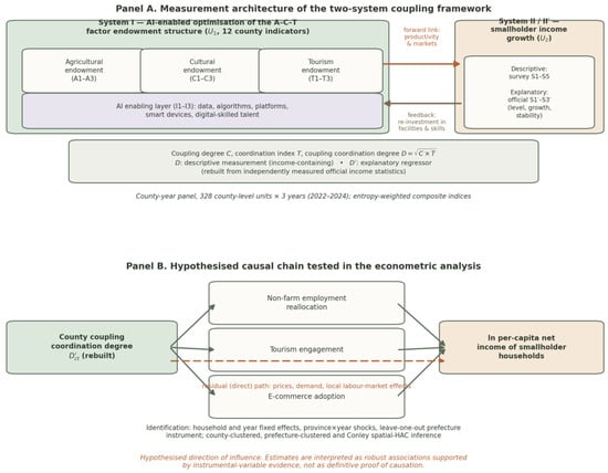
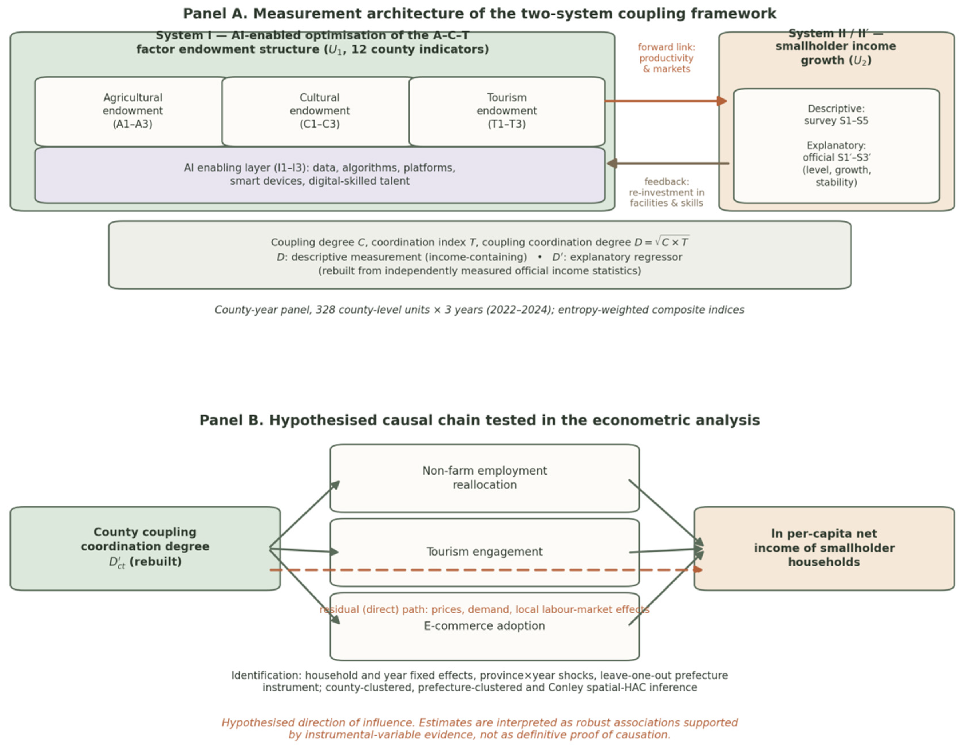
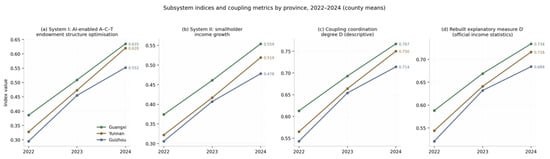
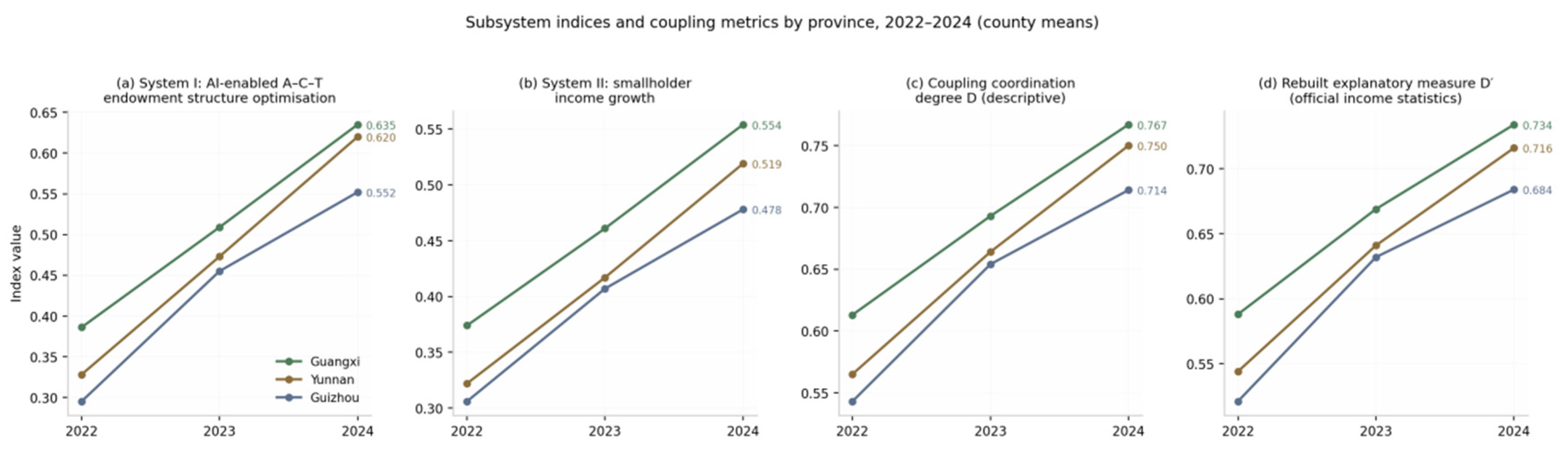
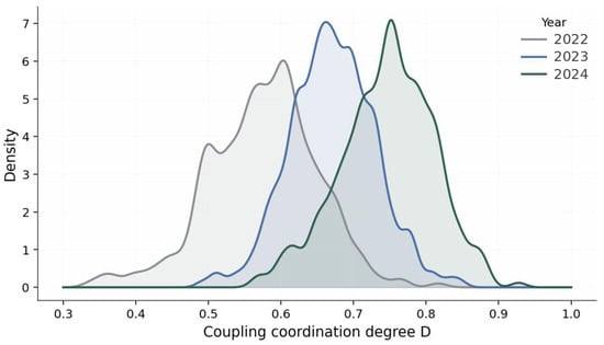
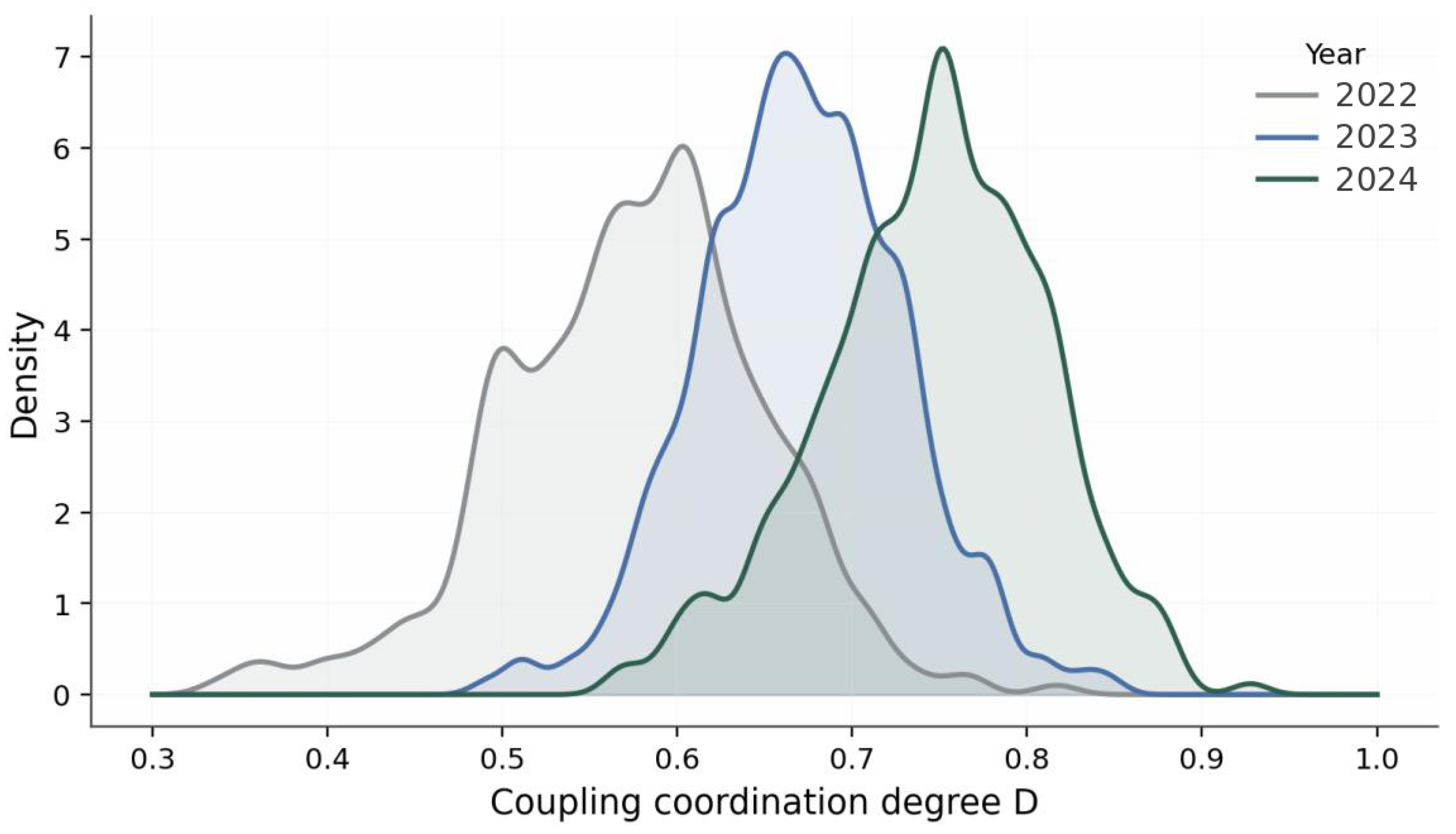
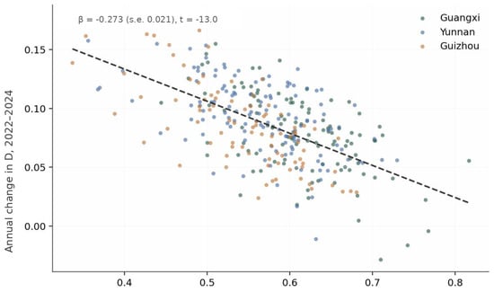
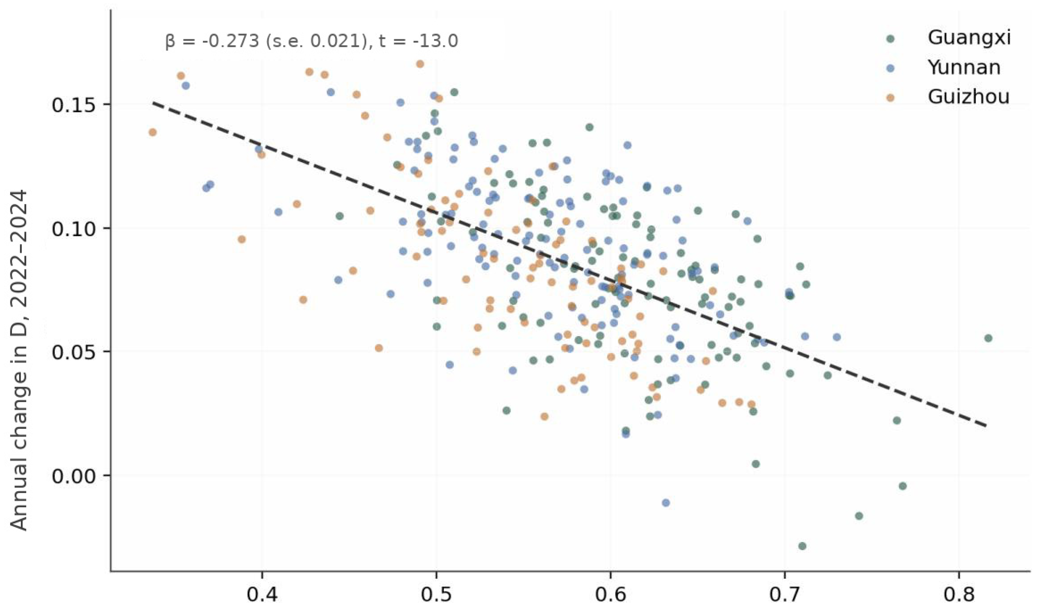
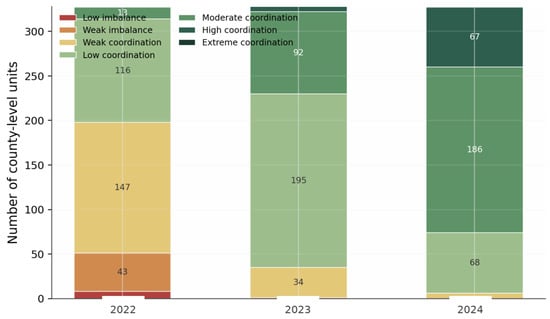
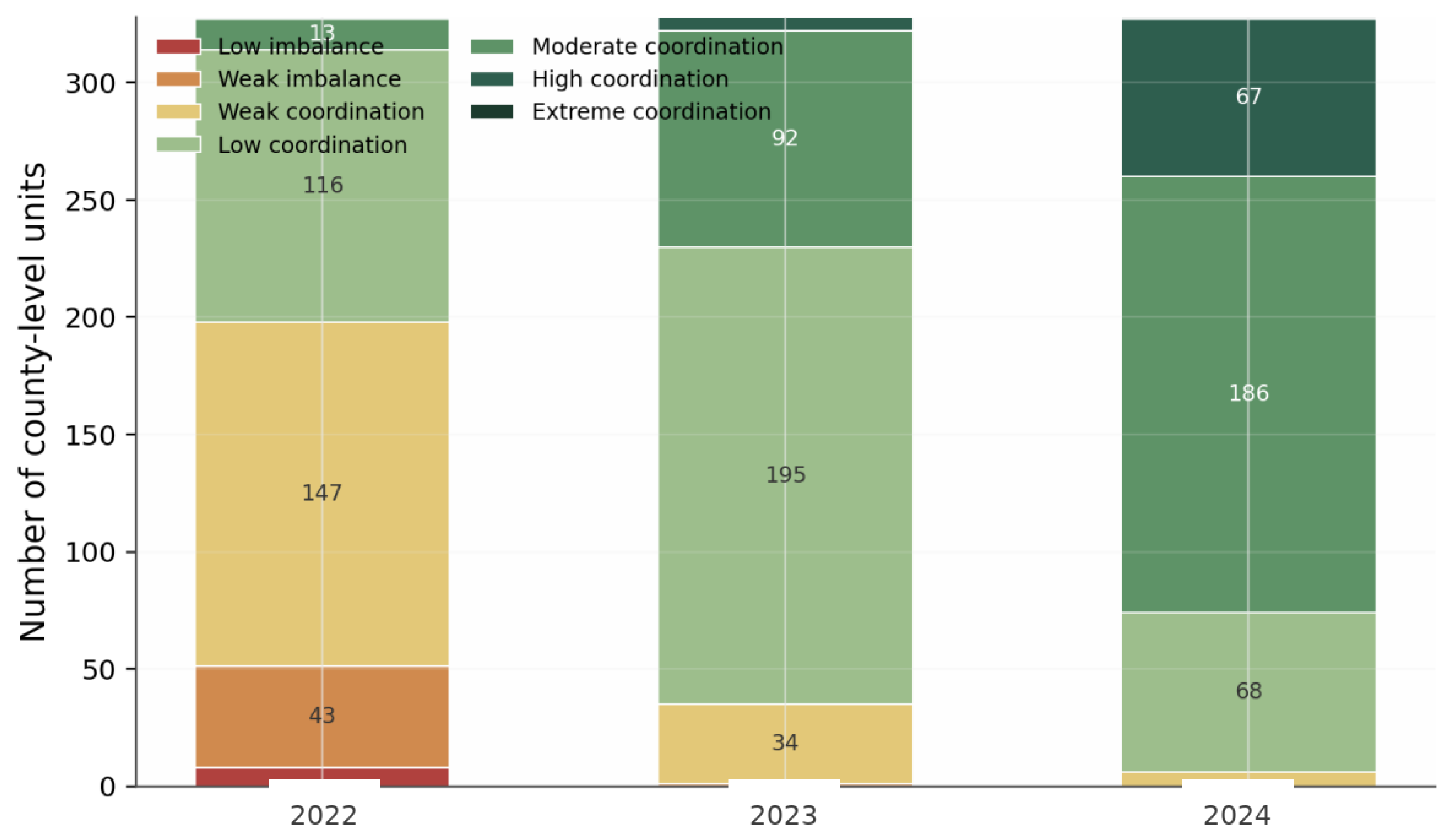
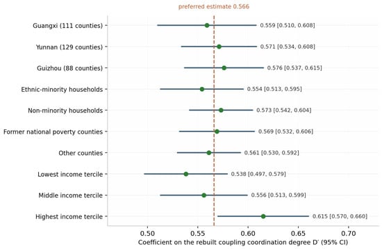
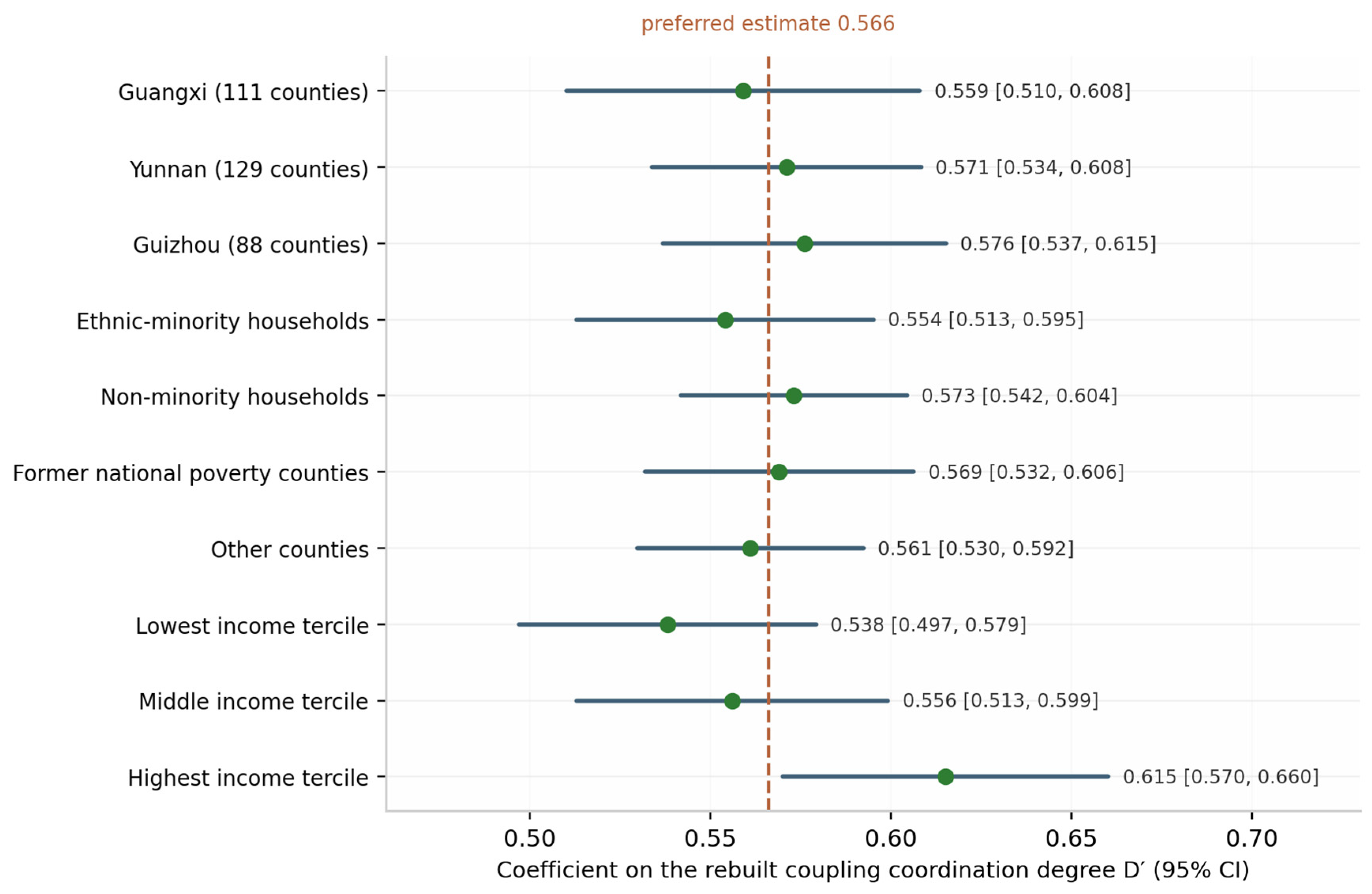

Disclaimer/Publisher’s Note: The statements, opinions and data contained in all publications are solely those of the individual author(s) and contributor(s) and not of MDPI and/or the editor(s). MDPI and/or the editor(s) disclaim responsibility for any injury to people or property resulting from any ideas, methods, instructions or products referred to in the content. |
© 2026 by the author. Licensee MDPI, Basel, Switzerland. This article is an open access article distributed under the terms and conditions of the Creative Commons Attribution (CC BY) license.