


Abstract
River ice is a characteristic feature of the temperate zone, yet its future decline remains poorly quantified. This study analyses ice regimes of two Central European rivers, the Pilica and Węgorapa, using 1965–2022 observations and projections to 2100 under SSP1-2.6, SSP3-7.0 and SSP5-8.5. Water temperature was estimated from seven-day mean air temperature with a simplified Mohseni model, and ice occurrence with an autologistic model. Over 1965–2022, the ice season shortened by 10.95 and 10.91 days per decade. By 2071–2100, mean ice-phenomena days are projected to decline to 10.9, 5.8 and 4.3 on the Pilica, and to 28.4, 14.9 and 10.2 on the Węgorapa under the three scenarios. The projections assume a stationary air–water temperature relationship and no continuation of the non-climatic decline beyond 2022; continuing the observed drift of that relationship would reduce ice-phenomena days by a further 4–10%. Because air–water coupling also depends on hydrological and physical factors not represented, the results indicate the direction and broad magnitude of change rather than future water temperature dynamics, and process-based thermal models are a priority for future research. Such losses may affect river ecosystems, water-resource management, river-valley infrastructure and energy production.
1. Introduction
Global warming is currently one of the most important—if not the single most important—problems facing our planet. The consequences of this process are already evident across many domains, affecting both the natural environment and human activities [1,2,3,4,5]. Importantly, however, humanity faces further challenges associated with the continued transformation of climatic conditions and, consequently, of the complex web of processes that depend on them. In this context, knowledge of the future responses of individual geosystems is essential, particularly for ensuring sustainable development. The hydrosphere is an important component of the natural environment and, through the hydrological cycle, connects its other components. In aquatic ecosystems at middle and high latitudes, the seasonality of ecosystem functioning is particularly important, as it is associated with the occurrence of ice phenomena. These phenomena constitute a key feature of the cold season, which—depending on latitude and local conditions—may vary considerably in duration and affect the functioning of inland waters in different ways [6,7]. Studies of river ice phenomena have been conducted for many years and address a wide range of issues. In general, they can be divided into two main strands: natural processes and the significance of river ice for human activities. For example, studies conducted in northern China demonstrated that ice cover significantly altered environmental conditions by reducing dissolved oxygen concentrations and water temperature while increasing total phosphorus concentrations [8]. In contrast, research based on data from a stream in central Sweden showed that the presence of ice cover may improve the energy balance and increase the extent to which stream-dwelling fish use available habitat during winter [9]. Measurements conducted in the Red River showed that the influence of ice cover is most pronounced near both banks, where the vertical velocity profile undergoes considerable modification. These findings are important, among other reasons, for understanding sediment transport in ice-covered rivers [10]. Prowse and Culp [11] highlighted the important role of river ice phenomena in flood formation, noting that they may occasionally be the dominant cause of flooding in cold regions. Ice-jam floods are important hydrological and hydraulic phenomena in the Northern Hemisphere and are a source of serious concern for a wide range of stakeholders [12].
In regions with cold climates, any changes in the hydroclimatic regime may significantly affect river ice processes [13]. A commonly observed pattern is a shortening of the ice season, as demonstrated by studies conducted in various parts of the world. Analyses of long-term trends in river ice phenology in Alaska (1979–2023) reveal a persistent reduction in the duration of ice cover, mainly due to later freeze-up, with statistically significant changes ranging from 3 to 5 days per decade [14]. The dates of ice-cover formation and complete freezing of the Heilongjiang River in Northeast Asia shifted to later dates, whereas the date of complete ice disappearance shifted to an earlier date, resulting in a shorter duration of ice cover [15]. In the case of Lithuanian rivers, two periods were distinguished: 1961–1990 and 1991–2020. During the latter period, the rivers froze, on average, nine days later, while the ice disappeared 24 days earlier than during the former period [16].
In Poland, river ice phenomena have been the subject of numerous previous studies [17,18,19,20,21,22,23]. To date, however, no projections of future changes in river ice phenomena have been developed, and addressing this gap is the focus of the present study. This approach advances the current state of knowledge and is consistent with the observations of Thellman et al. [24], who noted that knowledge of rivers during winter remains considerably less developed than knowledge concerning the growing season.
The main objective of this article is to determine future changes in the ice regimes of two lowland rivers in Poland under various climate scenarios projected through the end of the twenty-first century. This objective forms part of the broader global context of projections concerning river functioning and provides a point of reference for Central Europe. In this study, the term “nonlinear transformation” denotes a change in the ice regime that is not proportional to the warming that drives it. Three forms of such behaviour are examined: (i) a threshold response, in which a river passes from a regime with regular ice cover to one in which cover is rare while ice phenomena of some kind persist; (ii) a declining sensitivity, in which each additional degree of winter warming removes fewer days of ice as the remaining ice season shrinks; and (iii) a non-stationary relationship between air temperature and ice, in which the same winter temperature produces less ice than it did decades earlier.
2. Materials and Methods
The analysis proceeds in three connected stages: characterisation of the observed ice regime, calibration and validation of a daily ice model on that record, and projection of the model to 2100 under bias-corrected CMIP6 forcing. Figure 1 summarises the chain and the dependencies between stages.
Figure 1.
Processing chain, from the observational record and the ISIMIP3b forcing through to projections and deliverables.
2.1. Study Sites and Observational Data
The study uses daily records from two Polish rivers selected to contrast strongly in their present ice regime. The Pilica is gauged at Przedbórz (51.089° N, 19.875° E) in the lowlands of central Poland, with air temperature supplied by the Łódź synoptic station (51.723° N, 19.400° E). The Węgorapa is gauged at Mieduniszki (54.327° N, 21.980° E) in the more continental north-east, with air temperature from Kętrzyn (54.068° N, 21.369° E). The two catchments differ in size, setting and degree of lake influence. The Pilica gauge at Przedbórz stands at river kilometre 208.6, with a gauge datum of 187.4 m a.s.l., and closes a catchment of 2547 km2 within a total basin of 9258 km2; the river is the longest left-bank tributary of the Vistula, 342 km in length, and above the gauge it is effectively unregulated, with no lakes of significance and only minor structures in the headwaters. The Sulejów Reservoir, impounded in 1974, lies downstream of Przedbórz and therefore does not influence the record used here. The Węgorapa gauge at Mieduniszki stands at river kilometre 2.0, two kilometres above the Polish–Russian border, with a gauge datum of 86.3 m a.s.l., and closes 1586 km2. It lies on the outflow of Lake Mamry, the second-largest lake in Poland at 104 km2 and part of the Great Masurian Lakes; the river continues into the Kaliningrad region as the Angrapa and reaches the Baltic through the Pregolya. Its regime is consequently lake-influenced: the gauge integrates the storage and thermal inertia of the whole lake system, and a small early twentieth-century impoundment at Ołownik lies between the lake outflow and the gauge. The two sites also differ climatically. On the Köppen–Geiger classification [25], the Pilica site falls in the warm-temperate, fully humid, warm-summer class Cfb, while the Węgorapa site falls in the snow class Dfb, whose coldest month lies below −3 °C; the boundary between the two classes crosses Poland between the sites (Figure 2). Air temperature is taken from the nearest long-record synoptic station in each case, 78 km from the gauge for Łódź and 49 km for Kętrzyn, so the station series is used as a regional thermal forcing rather than as a local measurement. Site characteristics are collected in Table 1.
Figure 2.
Location of the analyzed rivers.
Table 1.
Study sites and completeness of the observational record, hydrological years 1965–2022. Catchment areas, river kilometres and gauge datums are from the IMGW-PIB station registry; completeness is computed over the full 1965–2022 window.
For each station, the record comprises daily water temperature, daily air temperature, and two binary ice variables. Ice phenomena denote the presence of any ice form in the channel—shore ice, slush, pack ice or complete cover—while ice cover denotes only the situation in which ice spans the full water surface and isolates it from the atmosphere. The two were analysed as separate targets throughout rather than combined, because they represent physically distinct states and, as the results show, they diverge sharply on the Pilica.
All data are organised by hydrological year, which begins on 1 November and ends on 31 October of the following year, so that each ice season falls within a single year rather than being split across the calendar boundary. The analysis covers hydrological years 1965–2022; air temperature availability gives 58 winters on the Pilica and 57 on the Węgorapa (Table 1). Onset and end dates were derived independently from the daily flags and cross-checked against the station ice-season records.
All observations are national monitoring data of the Institute of Meteorology and Water Management—National Research Institute (IMGW-PIB), which operates the Polish hydrological and meteorological service. Completeness over the study period is given in Table 1. On the Pilica, the air temperature, water temperature, and both ice flags are complete apart from a single missing day in 21,184. On the Węgorapa, the air temperature record begins in November 1965, so hydrological year 1965 has no forcing and is excluded; that river contributes 57 winters against 58 for the Pilica, and all other variables are complete. No gap filling was performed at any point: days without air temperature are dropped from the fits and from the derived indicators, which is preferable to interpolating the driver of a threshold process. The record is assumed homogeneous across the period. Ice phenomena are observed visually to a stable national protocol, but any undocumented change of observer or practice would project onto the decadal term introduced in Section 2.4 and could not be separated there from a physical trend. The implications of this assumption are discussed in Section 4.
2.2. Air–Water Temperature Coupling
Water temperature was related to air temperature using the four-parameter logistic function of Mohseni et al. [26], which is the standard parameterisation for stream thermal response,
where AT7 is the seven-day mean air temperature, μ and α are the lower and upper asymptotes, γ is the steepness at the inflection and β is the inflection temperature. The logistic form is used in preference to a linear fit because the relationship flattens as water temperature approaches 0 °C, which is precisely the range that governs ice formation. Parameters were estimated by non-linear least squares over the full 1965–2022 record.
WT = μ + (α − μ)/[1 + exp(γ(β − AT7))],
The four parameters were estimated by non-linear least squares on all paired daily observations within hydrological years 1965–2022, giving one curve per river with no seasonal or hysteresis term. The same curve is applied in calibration and in projection.
Fitted water temperature, rather than observed, is supplied to the ice model. This makes the projection chain run on air temperature alone—the variable climate models supply most reliably—while retaining a physically interpretable intermediate step, and it yields projected water temperature as a secondary result. Projections of river water temperature for the same Polish basins, against which this secondary output can be compared, are reported by Ptak et al. [27].
2.3. Ice Model
Daily ice occurrence was modelled with an autologistic generalised linear model (binomial family, logit link), fitted separately for each river and each of the two targets:
where P(icet = 1) is the probability that ice (ice phenomena or ice cover, fitted separately) is recorded on day t, and β0–β6 are coefficients estimated by maximum likelihood. AFDDt (°C·d) is the accumulation of freezing degree-days from 1 November to day t, reset at the start of each hydrological year. It enters as a square root following the classical result that ice thickness grows in proportion to the square root of accumulated freezing degree-days [28], so the predictor carries a physical form rather than an arbitrary one. AT7t and AT30t (°C) are the seven- and thirty-day mean air temperatures ending on day t, representing synoptic and seasonal thermal memory. (°C) is the water temperature on day t predicted from the Mohseni curve. icet−1 is the ice state (0 or 1) on the preceding day, which makes the model autologistic in the sense of Besag [29] and Zhu et al. [30]. Dt is time in decades relative to 2022 (D = 0 in 2022), whose role is set out in Section 2.4.
Because the lagged term is endogenous, the model is not evaluated pointwise but stepped forward in time. On each day, the linear predictor is formed using the model’s own simulated state on the preceding day, a probability is computed, and the new state is drawn from a Bernoulli distribution with that probability; the state is reset to zero at the start of each hydrological year. Each realisation is therefore one plausible sequence of winters rather than an expected value, and seasonal indicators—onset, breakup, duration, number of ice days and occurrence—are derived from the simulated daily sequences. Deriving them this way, rather than regressing dates on seasonal temperature as in the classical phenological analyses of Magnuson et al. [31], avoids the degenerate behaviour of date regression in winters when no ice forms, which is an increasingly common state on the Pilica. The choice of a statistical model driven by temperature and season, in preference to a process-based ice model, follows Yang et al. [32], whose equivalent formulation for global river ice reduced bias by 87% relative to a freezing-point criterion and so established that river ice responds to more than the position of the 0 °C isotherm. A process-based formulation was not adopted here because it would require, among others, channel geometry and radiative forcing that are neither available for these gauges nor projectable to 2100 with comparable confidence.
Coefficients were estimated by maximum likelihood, using iteratively reweighted least squares, on every daily observation of the calibration period. Because the lagged term makes residuals serially dependent within a winter, the asymptotic standard errors of such a fit understate uncertainty; standard errors and 95% intervals were therefore also obtained from a block bootstrap that resamples whole hydrological years with replacement (500 resamples), and those are the values reported. No conclusion in this paper rests on a coefficient p-value. Each projection uses 20 stochastic realisations per general circulation model and scenario, generated from a fixed random seed so that every number is exactly reproducible. For each of the resulting 100 members (5 GCMs × 20 realisations), each indicator is averaged over the period of interest, and the uncertainty intervals are the 10th and 90th percentiles across these 100 member means. The intervals therefore combine inter-model spread with the stochastic variability of the ice model; they do not include the uncertainty of the ice-model coefficients, which is quantified separately (Section 3.7, Table S1). To verify that 20 realisations are sufficient, the 2071–2100 projections were repeated with 200 realisations per GCM and scenario from an independent seed (Table S2). Ensemble means differed from the 20-realisation values by at most 0.34 days per winter and the 10th and 90th percentiles by at most 0.83 days, at most one-sixth of the corresponding interval; the Monte Carlo standard error of a 20-realisation ensemble mean is 0.01–0.26 days per winter. Seasonal indicators are defined identically for observations and for simulations: onset is the first hydrological day of a winter carrying the flag, breakup the last, duration the span between them inclusive of any ice-free interruption, and ice days the count of flagged days, which falls below the duration whenever a season breaks into separate spells. Onset, breakup, and duration are undefined in a winter without ice, so they are averaged over winters with ice only and are reported alongside the proportion of winters in which no ice occurs.
2.4. Treatment of Non-Stationarity
Whether the relationship between air temperature and ice occurrence is stationary over the record was tested by calibrating the model on an early window (1965–1999) and simulating the later period, then calibrating on a late window (1994–2022) and simulating the earlier period. A bias of consistent sign in both directions would indicate a mis-specified predictor set; a bias that reverses sign with the direction of extrapolation instead indicates that the relationship between air temperature and ice has itself shifted over the record. The decadal term D was introduced to absorb any such shift, and its contribution was assessed by refitting with and without it. D is an empirical representation of unresolved temporal non-stationarity: it captures the part of the decline in ice occurrence that the temperature predictors do not explain, and it is not attributed to any specific physical mechanism. Its coefficient therefore carries no process interpretation beyond the direction and size of that residual drift.
In projection, D is held at its 2022 value, so the model carries the present-day state of each river forward without extrapolating the residual drift beyond the end of the record. This corresponds to the assumption that the non-climatic component of the decline stops in 2022, and all projections in this paper are conditional on it. It was preferred to continuing the fitted trend for three reasons: continuing it would extend a linear trend 78 years beyond the data, which at unchanged temperature would reduce the odds of ice on a given day by a factor of 2.5–17.5 by 2100; it would impose the same non-climatic decline on every emission pathway; and, without an identified mechanism, there is no basis for assuming that the drift persists at its historical rate, stops, or reverses. The sensitivity of the projections to this choice is quantified in Section 3.7 (Table S3).
2.5. Climate Forcing and Bias Correction
Future daily near-surface air temperature was taken from the ISIMIP3b bias-adjusted CMIP6 archive (Inter-Sectoral Impact Model Intercomparison Project, Potsdam Institute for Climate Impact Research, Potsdam, Germany) at 0.5° resolution, produced with the trend-preserving ISIMIP3BASD v2.5 method against W5E5 v2.0 over 1979–2019 [33,34]. W5E5 comprises WFDE5 over land, itself a bias-adjusted ERA5 product [35,36]. Five general circulation models participating in CMIP6 [37] were used—GFDL-ESM4, IPSL-CM6A-LR, MPI-ESM1-2-HR, MRI-ESM2-0 and UKESM1-0-LL—under the SSP1-2.6, SSP3-7.0 and SSP5-8.5 pathways of ScenarioMIP [38]. ISIMIP3b does not provide SSP2-4.5, so SSP3-7.0 serves as the intermediate pathway; this also aligns the study with the wider ISIMIP impacts literature. The single grid cell containing each meteorological station was extracted server-side.
ISIMIP3b is adjusted to the W5E5 grid rather than to individual stations, so a residual grid-cell-to-point bias remains, concentrated in the part of the temperature distribution in which ice forms. A second-stage empirical quantile mapping was therefore applied, computed per calendar month over the 1979–2014 overlap and applied unchanged to every scenario [39]. Quantile mapping rather than a mean offset was chosen because the residual bias proved to be quantile-dependent rather than uniform; a more elaborate correction was not required, because air temperature is the only forcing variable and no inter-variable consistency constraint applies, and because quantile mapping is adequate for a near-Gaussian variable [40]. Because a correction that distorted the warming trend would invalidate the projections, signal preservation was verified rather than assumed [41].
The five models were propagated separately rather than combined into a weighted ensemble, so that inter-model spread is carried through to the projected ice indices. The full projection ensemble comprises 5 GCMs × 3 scenarios × 20 stochastic realisations over 78 hydrological years.
2.6. Validation Design
Three tests were applied, each addressing a different failure mode. The first is an out-of-sample test of the ice model; the third is a historical-period evaluation of the full forcing–model chain. First, the ice model was calibrated on 1965–1999 and simulated forward through 2000–2022 driven by temperature alone, with the model feeding its own simulated ice state back as the persistence term so that no observed ice entered the validation period. The validation period is warmer than the calibration period, so this tests the model in the direction in which it is subsequently extrapolated. One-step-ahead skill conditioned on the observed persistence term is also computed, but only as a diagnostic, because it is not the quantity a projection depends on.
Second, a random forest [42] was fitted to the same predictors and calibration window as a benchmark. It was not used for projection, since tree ensembles cannot extrapolate beyond their training range and late-century winters lie outside anything in the observational record.
Third, the full chain was evaluated over the historical period: the ice model was driven with bias-corrected ISIMIP historical forcing over 1979–2014, and the resulting distribution of seasonal ice days was compared with observations using a two-sample Kolmogorov–Smirnov test [43]. Because the quantile mapping was calibrated on the same 1979–2014 period and the ice model used for projection is fitted to the full record, this is a historical-period evaluation rather than an independent validation. It tests whether the chain reproduces the observed ice-day distribution when driven by climate-model output instead of station data, not whether the corrected forcing is skilful outside its calibration period. Free-running climate models are not initialised to observed years, so year-to-year correspondence carries no information, and only the distribution is testable.
Trends in observed indicators were assessed with the Mann–Kendall test [44] and quantified with the Theil–Sen slope estimator [45], both non-parametric and robust to the occasional extreme winter. Significance is reported at α = 0.05.
2.7. Sensitivity to the Bias-Correction Method
To establish how much the choice of bias correction influences the projections, the ice model was driven by three forcings—ISIMIP3b as delivered, the monthly quantile mapping described above, and a deliberately cruder monthly mean shift—and the 2071–2100 projections were recomputed. The spread across these three was then compared with the spread across the five GCMs and across the three emission pathways.
2.8. Data and Code Availability
The observational records are national monitoring data of IMGW-PIB and are available through the institute’s public data portal at danepubliczne.imgw.pl and traditional hydrological yearbooks. The ISIMIP3b bias-adjusted climate forcing is available from the ISIMIP repository under the ISIMIP terms of use [34]. The complete analysis pipeline—data preparation, air–water model, ice model, station-level bias correction, projections, validation, tables and figures—is implemented in Python 3.11.13 (Python Software Foundation, Wilmington, DE, USA). The Mohseni curve was fitted with SciPy 1.16.1 (scipy.optimize), the autologistic model with statsmodels 0.14.5, the random-forest benchmark with scikit-learn 1.7.1, the Mann–Kendall and Theil–Sen statistics with pyMannKendall 1.4.3, and data handling and figures used pandas 2.3.2, NumPy 2.2.6, xarray 2025.9.0 and Matplotlib 3.10.6. The pipeline is openly available, together with the derived data, from Figshare [46].
3. Results
3.1. Observed Changes, 1965–2022
Both rivers show a strong and statistically significant contraction of the ice season over the 58-year record (Table 2 and Table 3, Figure 3 and Figure 4).
Table 2.
Observed ice indicators by period (mean days per winter).
Table 3.
Observed trends in ice, thermal, and freezing indicators, hydrological years 1965–2022. Slopes are Theil–Sen estimates per decade and p-values are from the Mann–Kendall test; n is the number of winters in which the indicator is defined, which falls below the record length for onset, breakup and duration because those are undefined in a winter without ice. Hydrological days are counted from 1 November. The Theil–Sen slope for days with ice cover on the Pilica is zero because 43 of the 58 winters carry no ice cover at all, so the median of the pairwise slopes is zero even though the Mann–Kendall test detects a significant decline.
Figure 3.
Observed daily ice occurrence by hydrological year and hydrological day, 1965–2022. (Left) ice phenomena; (Right) ice cover. (Top) Pilica at Przedbórz; (Bottom) Węgorapa at Mieduniszki. The hydrological year begins on 1 November.
Figure 4.
Observed seasonal ice indicators with Theil–Sen trend lines, 1965–2022. Slopes and Mann–Kendall p-values are given in Table 3. (Top) Pilica; (Bottom) Węgorapa.
The duration of the ice season declined by 10.95 days per decade on the Pilica (p = 0.0001) and 10.91 days per decade on the Węgorapa (p = 0.0002). The number of days with ice phenomena fell by 7.08 and 9.12 days per decade, respectively (p < 0.001 in both cases). The season contracted from both ends: onset moved later by 6.44 days per decade on the Pilica and 5.00 days per decade on the Węgorapa, and the final ice day moved earlier by 4.57 and 4.42 days per decade.
The thermal context is consistent across the two catchments. November–April air temperature rose by 0.37 °C per decade on the Pilica and 0.42 °C per decade on the Węgorapa, and the corresponding water temperatures by 0.34 and 0.29 °C per decade. Accumulated freezing degree-days declined by 20.1 and 27.4 °C·d per decade. These rates are consistent with the declines reported for rivers in Poland. An analysis of two gauging stations on the Biebrza River in northeastern Poland covering the period 1959–2023 revealed a decline in river ice phenomena at a rate of 3 days per decade [47]. In the case of three rivers located in the coastal zone of the Baltic Sea, the timing of ice phenomena changed at a rate of 3 to 7 days per decade over the past sixty years [48].
The two rivers differ sharply in ice cover. On the Węgorapa, days with ice cover declined significantly, by 5.00 days per decade (p = 0.0067), from a mean of 36.7 days per winter in 1965–1994 to 18.0 in 1995–2022 and 14.4 in the last decade. On the Pilica, ice cover had already become rare early in the record and has since all but disappeared: the mean fell from 5.8 days per winter in 1965–1994 to 1.6 and then 0.3 days, and the proportion of winters with no ice cover at all rose from 63% to 86% and then 90%. Over the full record, the Pilica recorded no ice cover in 43 of 58 winters, including nine of the last ten; the Węgorapa in 12 of 57. Trends in ice-cover onset, breakup and duration are not significant on either river, which reflects the small and shrinking number of winters in which those dates are defined at all—15 on the Pilica—rather than an absence of change.
Read as a whole, Table 3 describes a season contracting from both ends rather than breaking apart internally. Onset is the more mobile end, moving later by 6.44 days per decade on the Pilica and 5.00 on the Węgorapa against 4.57 and 4.42 days per decade for the final ice day, so roughly three-fifths of the lost season is lost at the beginning of winter. The span shortens faster than the number of ice days within it—10.95 against 7.08 days per decade on the Pilica—which invites the reading that the season is fragmenting, but the proportion of the span that actually carries ice shows no trend on either river (0.55 in 1965–1993 against 0.51 in 1994–2022 on the Pilica, and 0.75 against 0.74 on the Węgorapa; Mann–Kendall p = 0.42 and 0.67). The observed record therefore documents a shorter ice season of unchanged internal character, and the fragmentation that appears in the projections has no clear precedent in it. Under similar warming (0.37 and 0.42 °C per decade, with freezing degree-days falling by 20.1 and 27.4 °C·d per decade), the Pilica lost proportionally more of its ice than the Węgorapa. Finally, the indicators that fail significance in Table 3 are precisely those defined only in winters that still produce ice cover—15 winters on the Pilica against 45 on the Węgorapa—so their non-significance measures the loss of statistical power that the decline itself has caused, and should not be read as stability. Because a cold winter tends to follow a cold winter, the independence that the Mann–Kendall test assumes is not strictly met—the lag-1 autocorrelation reaches +0.45 for Węgorapa air temperature and +0.37 for its ice-season duration—so every p-value in Table 3 was recomputed with the Hamed–Rao variance correction [49]. Not one verdict changes at α = 0.05 in any of the 22 series, and for several the corrected value is the smaller of the two, so the trends reported here are not artefacts of serial correlation (Table S4).
Table S1 describes the same winters in terms of their internal structure. The longest unbroken spell of ice phenomena shortened on both rivers, from 23.6 to 14.0 days on the Pilica and from 55.7 to 37.9 days on the Węgorapa between the first and the last 28 years of the record (−4.00 and −7.14 days per decade, p = 0.0002 and 0.0030), and continuous ice cover shortened with it, from 30.6 to 17.1 days on the Węgorapa (−4.00 days per decade, p = 0.0024). The number of separate spells did not rise. It fell on the Pilica, from 4.3 to 3.3 per winter with ice (−0.43 per decade, p = 0.0046), and is statistically unchanged on the Węgorapa (p = 0.56). Taken with the stable ice fraction reported above, this settles what kind of change the record contains: the ice season is being removed from its ends and thinned in its longest episodes, not perforated into a larger number of short ones.
Onset and end dates derived independently from the daily flags reproduce the station ice-season records to within a mean of 2.1 days on the Pilica and 1.1 days on the Węgorapa, confirming that the daily flags and the station ice-season records describe the same seasons.
3.2. Air–Water Coupling and Its Drift
The Mohseni function reproduces observed water temperature closely at both stations, explaining 94.7% of the variance on the Pilica (RMSE 1.50 °C) and 96.8% on the Węgorapa (RMSE 1.30 °C) (Table S5, Figure 5a).
Figure 5.
Air–water temperature coupling and its drift. (a) Observed daily water temperature against seven-day mean air temperature, with the fitted Mohseni curves. (b) Annual mean November–April Mohseni residual (modelled minus projected water temperature) with Theil–Sen trends. (c) Mean water temperature on days with AT7 below −2 °C, 1965–1993 (pale) and 1994–2022 (solid).
The relationship is nevertheless not stationary. The residual rises by 0.083 °C per decade on the Pilica (p = 0.026) and 0.033 °C per decade on the Węgorapa (p = 0.036), indicating that water is progressively warmer than the historical air–water relationship implies (Figure 5b). Restricted to days with AT7 below −2 °C, mean water temperature on the Pilica rose by 0.27 °C between the two halves of the record, against 0.03 °C on the Węgorapa (Figure 5c).
3.3. Non-Stationarity of the Temperature–Ice Relationship
A model containing only temperature predictors proved to be biased in both temporal directions. Calibrated on 1965–1999 and simulated forward, it over-predicted ice phenomena over 2000–2022 by 13.3 days per winter on the Pilica and 10.2 days on the Węgorapa; calibrated instead on 1994–2022 and simulated backward, it under-predicted the earlier period by 15.2 and 13.8 days, respectively (Table S6). A bias of consistent sign would suggest a mis-specified predictor set, but a bias that reverses with the direction of extrapolation indicates that the relationship between air temperature and ice has itself shifted over the record. The Akaike information criterion is close to indifferent between the two formulations (Table S6): the two differ by four units or less in six of the eight fits, so the case for the decadal term rests on the two-directional bias rather than on in-sample fit, as is expected of a term that corrects a drift between periods rather than the fit within one of them.
Part of the change is visible in the air–water coupling, whose drift is reported in Section 3.2: at fixed air temperature the water is progressively warmer than the historical relationship implies, and on days cold enough to matter for ice formation (AT7 < −2 °C) mean water temperature on the Pilica rose from 0.34 °C in 1965–1993 to 0.61 °C in 1994–2022.
The decadal term D absorbs this residual change. At fixed air temperature, the odds of ice on a given day decline by 14.5% per decade on the Pilica and 11.2% per decade on the Węgorapa for ice phenomena, and by 30.7% and 12.4% for ice cover. Including the term reduces the forward validation bias for ice phenomena from 13.3 to 7.9 days on the Pilica and from 10.2 to −1.4 days on the Węgorapa.
How much of that decline the air–water drift explains can be measured rather than asserted. Refitting each model with the observed water temperature of the same day in place of the modelled value—so that the drift documented in Section 3.2 enters the model directly instead of being masked by a stationary Mohseni curve—leaves the decadal term almost intact. The odds ratio per decade moves from 0.855 to 0.876 for Pilica ice phenomena and from 0.693 to 0.699 for Pilica ice cover, and on the Węgorapa from 0.888 to 0.894 and from 0.876 to 0.877, so the drift accounts for 15.1% of the decadal term in the first case and between 0.3% and 5.2% in the other three. The air–water drift therefore accounts for only a small part of the decadal term; the remainder is not explained by the thermal predictors in the model and is represented here only empirically.
3.4. Ice Model Performance
Table 4 reports the fitted coefficients of all four models with block-bootstrap standard errors. The persistence term dominates every model, raising the odds of ice by two to three orders of magnitude when ice was present on the preceding day, which is why the model must be stepped forward in time rather than evaluated pointwise. The temperature terms are negative throughout, as expected, but they are mutually collinear—the seven-day mean, the thirty-day mean and the modelled water temperature are all functions of the same air-temperature series—so the division of the thermal signal between them is not identified and five of the twelve individual bootstrap intervals span zero even though their joint contribution is well determined. The accumulated freezing degree-day term is also negative once those terms are present, and should not be read as a physical statement that accumulated cold suppresses ice: AFDD rises monotonically through a winter, so conditional on current temperature it also encodes elapsed season, and a late-winter day carrying a large accumulation is indeed less likely to be icy than an equally cold day in December. The decadal term is the only coefficient on which an interpretation is placed in this paper, and its bootstrap interval excludes zero in all four models. Block-bootstrap standard errors are 1.0 to 1.9 times the asymptotic ones, confirming that the 21,000 daily observations are far from independent. One further check is needed because ice cover is rare—it occurs on 1.03% of days on the Pilica—and maximum-likelihood logistic regression is biased away from zero when events are rare. Refitting all four models with Firth’s penalised likelihood [50] moves no coefficient by more than 0.26 of its bootstrap standard error, so that bias is negligible at these event rates and the maximum-likelihood fit is retained.
Table 4.
Fitted autologistic ice-model coefficients, calibration 1965–2022, with block-bootstrap standard errors in parentheses (500 resamples of whole hydrological years). The decadal term is expressed per decade relative to 2022; its odds ratio is given separately for interpretation.
Under free-running validation, the full model reproduces the 2000–2022 period with a bias of −1.4 to +7.9 days per winter for ice phenomena and −1.6 to +5.2 days for ice cover (Table S7, Figure S1). Adding the decadal term improves every ice-phenomena statistic: bias falls from +13.3 to +7.9 days on the Pilica and from +10.2 to −1.4 days on the Węgorapa, with mean absolute error falling from 16.1 to 12.0 and from 17.5 to 12.9 days.
One-step-ahead skill conditioned on the observed persistence term is far higher than the free-running result, reaching AUC 0.985–1.000 across the four river–variable combinations; it is reported here only as a diagnostic. On that same measure, the random-forest benchmark matches the generalised linear model, at 0.984 against 0.985 for Pilica ice phenomena and 0.993 against 0.994 for the Węgorapa, so no discrimination is sacrificed by preferring the parsimonious formulation.
3.5. Performance of the Climate Forcing and Bias Correction
Before the station-level correction, the ISIMIP3b forcing carried errors of very different magnitude at the two sites. On the Pilica, the residual grid-cell-to-point bias was a warm one, averaging +0.50 °C over November–April and reaching +0.9 °C through the cold-to-mid range of the distribution (Table 5, Figure S2a), that is, precisely the range in which ice forms.
Table 5.
Distributional hindcast, 1979–2014, driven by bias-corrected ISIMIP historical forcing.
It was seasonally concentrated, peaking at +0.89 °C in February and exceeding +0.4 °C in every month from December to March (Figure S3c). The consequence for an ice study is direct: the raw forcing produced 6.1 percentage points too few days below 0 °C over the season as a whole, with 6.0 to 9.9 percentage points missing in each month from November to March (Figure S3b). On the Węgorapa, the raw forcing was already close to the station record, with a November–April mean bias of −0.09 °C, monthly biases within ±0.20 °C except in April (−0.49 °C), and a frost-day error of only +0.35 percentage points.
After correction, the November–April means match the station records to within 0.02 °C on both rivers—1.87 °C against 1.85 °C observed on the Pilica, where the raw forcing gave 2.35 °C, and 0.98 °C against 0.96 °C on the Węgorapa—and the 1st and 5th percentiles to within 0.15 °C (Tables S8 and S9). Because a correction that distorted the warming trend would invalidate the projections, signal preservation was verified rather than assumed, since quantile mapping can distort a projected trend if applied carelessly [41]: November–April warming for 2071–2100 relative to 1985–2014 changes by at most 0.054 °C between the raw and corrected series across all rivers and scenarios (Table S9). The correction therefore removes the offset without touching the climate change signal it is applied to.
Across the ten distributional metrics of Table 5, the correction improves every one on both rivers. The decisive metric for this study is the frequency of days below 0 °C, which on the Pilica moves from −6.12 to −0.32 percentage points; Figure S3b shows the improvement acting in the months in which the ice season is decided, the corrected series matching the observed monthly frost frequency to within 1.2 percentage points in all six months, and Figure S3c shows the monthly mean bias falling to at most 0.05 °C. Cold-tail percentile errors on the Pilica fall from +0.48 and +0.75 °C at the 5th and 10th percentiles to +0.02 °C at both; the standard-deviation ratio moves from 0.977 to 1.001, the Perkins skill score rises from 0.908 to 0.933; and the Kolmogorov–Smirnov statistic falls from 0.075 to 0.015. Distribution shape and seasonal timing improve on both rivers: the quantile–quantile R2 rises from 0.9954 to 0.9996 on the Pilica and from 0.9980 to 0.9998 on the Węgorapa, and the seasonal-cycle R2 rises from 0.936 to 0.942 and from 0.935 to 0.939. On the Węgorapa, where the raw forcing was already close to the station record, the gains are correspondingly smaller—mean bias from −0.09 to +0.02 °C, Kolmogorov–Smirnov statistic from 0.026 to 0.013, Perkins score from 0.937 to 0.940—so the correction is substantial where it was needed and close to neutral where it was not. The correction behaves consistently across the five models: model by model, the corrected mean bias stays within 0.07 °C and the Kolmogorov–Smirnov statistic within 0.026, so no single general circulation model drives the result (Supplementary Table S10). The models are not equally biased to begin with: on the Pilica the raw frost-day deficit ranges from 3.6 percentage points for MRI-ESM2-0 to 8.5 for UKESM1-0-LL, and the correction compresses that five-point disagreement to 1.7 points, so it also removes most of the inter-model disagreement about how often the river reaches freezing.
In the historical-period evaluation, driven by bias-corrected ISIMIP historical forcing over 1979–2014, the model reproduces the observed distribution of seasonal ice days on all four river–variable combinations, with no Kolmogorov–Smirnov test rejecting at α = 0.05 (p = 0.31–0.91; Table 5, Figure S2b,c,e,f). Simulated means are 27.4 against 31.2 observed days for Pilica ice phenomena and 55.3 against 59.0 for the Węgorapa, with standard deviations of 17.6 against 21.9 and 26.0 against 26.9 days, so the year-to-year variability of the ice season is reproduced as well as its mean. The proportion of winters without ice cover is reproduced to within four percentage points on both rivers. This end-to-end agreement is distributional by design: because free-running GCMs are not initialised to observed weather, a year-by-year or day-by-day match is not expected and would not be evidence of skill—the apparent day-to-day correlation of +0.39 between the corrected forcing and the station record collapses to +0.007 on the Pilica and −0.001 on the Węgorapa once the shared seasonal cycle is removed. Because the bias correction and the ice model were both fitted on data that include 1979–2014, this agreement shows that the GCM-driven chain is consistent with the observed ice-day distribution, but it is not an out-of-sample test; out-of-sample skill rests on the free-running 2000–2022 validation (Section 3.4).
Because the projections also state when the ice season runs, the hindcast was repeated for timing (Table S11). Onset is reproduced everywhere: the bias runs from −7.2 to +0.3 days across the four river–variable combinations, and no Kolmogorov–Smirnov test rejects (p = 0.25–0.92). Breakup and duration are reproduced on the Węgorapa (p = 0.11–0.96) but not for Pilica ice phenomena, where the simulated season ends 18.8 days too late and lasts 23.8 days too long, with a simulated spread nearly twice the observed one (p = 0.002 and 0.001). Projected onset on both rivers, and all three timing indicators on the Węgorapa, can therefore be read at face value, while projected Pilica breakup and duration should be treated as indicative. The ice-day totals on which the conclusions of this study rest are unaffected, since they are evaluated separately in Table 5.
3.6. Projected Changes to 2100
Projected ice indices decline under every scenario on both rivers, with the separation between scenarios emerging after about 2050 (Figure 6, Table 6).
Figure 6.
Projected ice indices to 2100 under three emission pathways. Black, observed (thin line, annual values; thick line, ten-year running mean). Coloured lines, ensemble mean of ten-year running means across the 100 members (5 GCMs × 20 stochastic realisations); shading, 10th–90th percentile across these members. The dotted vertical line marks the end of the observational record.
Table 6.
Projected mean days per winter, 2071–2100, and the percentage of winters with no occurrence. Values in parentheses are the 10th–90th percentiles across the 100 ensemble members (5 GCMs × 20 stochastic realisations), each averaged over 2071–2100; they combine inter-model spread and the stochastic variability of the ice model. Parameter uncertainty is reported separately in Table S1. All values assume that the decadal term remains at its 2022 value (Section 2.4).
On the Pilica, mean days with ice phenomena fall from 22.0 per winter in 1995–2022 to 10.9 (10th–90th percentile 6.0–15.4) under SSP1-2.6, 5.8 (2.6–9.2) under SSP3-7.0 and 4.3 (1.3–6.9) under SSP5-8.5 by 2071–2100, reductions of 50%, 74% and 81%. Ice cover, already near zero, becomes effectively absent: 0.3 (0.0–0.8), 0.2 (0.0–0.5) and 0.1 (0.0–0.2) days per winter, with 95.0%, 96.9% and 98.1% of winters carrying no ice cover at all. The scenario makes little difference to this outcome.
On the Węgorapa, the trajectory is scenario-dependent. Days with ice phenomena fall from 48.2 in 1995–2022 to 28.4 (15.9–39.8), 14.9 (7.2–23.5) and 10.2 (2.5–17.5) by 2071–2100 across the three pathways, and days with ice cover from 18.0 to 8.7 (3.4–15.1), 3.9 (1.2–6.9) and 2.5 (0.5–4.9). The proportion of winters with no ice cover rises from 32% observed in 1995–2022 to 50.2% under SSP1-2.6, 68.2% under SSP3-7.0 and 75.2% under SSP5-8.5 (Figure 7). Under strong mitigation, the Węgorapa therefore retains an intermittent but recurrent ice-cover regime, whereas under the high-emission pathway ice cover becomes the exception rather than the norm.
Figure 7.
Loss of ice cover and contraction of the ice season. Percentage of winters with no ice cover by decade, observed and projected (Left Column), daily probability of ice phenomena by hydrological day for 2023–2040 and 2071–2100 under each pathway (Centre and Right Columns).
Complete absence of ice of any kind also becomes common. By 2071–2100 the proportion of winters with no ice phenomena reaches 9.3%, 24.2% and 32.2% on the Pilica and 6.8%, 22.1% and 33.3% on the Węgorapa across the three scenarios. The daily probability fields (Figure 7) show that the season not only shortens but fragments: peak mid-winter probability falls well below unity, so a continuous ice season is replaced by intermittent episodes even in winters that still record ice.
Table S12 sets the end-century figures against the two earlier periods. Until about 2040 the three pathways are barely distinguishable—13.6, 12.2 and 13.2 days of ice phenomena per winter on the Pilica and 34.4, 30.0 and 33.8 on the Węgorapa. The separation appears in 2041–2070 and widens to the end of the century: on the Węgorapa, ice phenomena fall to 28.1, 20.2 and 20.3 days by mid-century and then to 28.4, 14.9 and 10.2 by 2071–2100, so that under strong mitigation the mid-century state is essentially held to 2100 while under the two higher pathways it halves again.
The ice season not only shortens, but also shifts. Table 7 reports onset, breakup, and duration for the winters in which ice still forms. On the Węgorapa, ice phenomena presently begin on 21 December on average and end on 27 February, a span of 69.5 days; by 2071–2100 onset is 6.6 days later under SSP1-2.6 (10th–90th percentile across members: 3.4 days earlier to 20.1 days later), 18.3 days later under SSP3-7.0 (8.0–32.8 days later) and 20.8 days later under SSP5-8.5 (10.3–41.2 days later), while breakup advances by 9.6 days under SSP3-7.0 (from 0.8 days later to 20.4 days earlier) and 12.7 days under SSP5-8.5 (2.3–24.1 days earlier), so the span contracts by 6.3, 27.9 and 33.5 days respectively. The Pilica shows the same delay in onset—3.2 (6.1 days earlier to 15.8 days later), 14.7 (2.5–32.9 days later) and 16.3 (4.2–39.3 days later) days across the three pathways—with breakup almost unchanged (0.5 days earlier under SSP5-8.5; members range from 15.5 days earlier to 18.0 days later), and its ice-phenomena span contracts by up to 16.8 days. Ice cover, where it survives at all, becomes a brief mid-winter episode: its mean span falls from 30.9 days to 24.7, 17.0 and 14.6 days on the Węgorapa, and from 11.2 days to between 6.7 and 3.0 days on the Pilica. These timing shifts are conditional on ice occurring and must be read together with the proportion of winters in which it does not, which by 2071–2100 under SSP5-8.5 reaches 32.2% of winters for Pilica ice phenomena and 75.2% for Węgorapa ice cover. The Pilica ice-cover figures for 2071–2100 rest on the 2–5% of winters that still produce cover and are indicative only. Table S11 shows that breakup and duration on the Pilica are the two indicators the model does not reproduce distributionally, so the Pilica timing shifts in particular should be read as indicative.
Table 7.
Ice-season timing, observed 1995–2022 and projected 2071–2100. Onset and breakup are means over winters in which ice occurs; duration is the span from onset to breakup inclusive, and therefore exceeds the number of ice days when a season breaks into separate spells.
Table 8 converts those trajectories into dates. Complete ice cover on the Pilica has effectively already gone: its decadal mean falls below half the 1995–2022 value in the 2020s under every pathway, and more than half of the winters in that same decade carry none at all. On the Węgorapa, ice cover crosses the half-loss threshold in the 2020s under SSP3-7.0, the 2040s under SSP5-8.5, and the 2050s under SSP1-2.6, and the majority of winters are already free of ice cover from the 2020s under the two lower pathways. Ice phenomena are far more persistent. Their half-loss decade is the 2040s or 2050s in every case, but no pathway takes either river to a majority of ice-free winters before 2100: by the 2090s under SSP5-8.5 the proportion reaches 40.0% on the Pilica and 42.9% on the Węgorapa. The distinction matters for how the results should be read. Complete ice cover is a threshold already being crossed, and on the Pilica the crossing is essentially complete regardless of mitigation; the disappearance of ice altogether remains, even under the strongest forcing considered here, an end-of-century possibility rather than a projected outcome.
Table 8.
Time of emergence of the projected ice loss. The half-loss decade is the first decade whose mean falls below half the observed 1995–2022 mean; the majority ice-free decade is the first in which more than half of the winters carry no ice of the kind named. Decades run from the 2020s (2023–2030) to the 2090s (2091–2100); a dash means the threshold is not crossed before 2100.
Table S13 carries the same structural question into the projections. The longest unbroken spell of ice phenomena falls from 37.9 days observed to 20.2, 11.0 and 7.8 days by 2071–2100 on the Węgorapa, and from 14.0 to 6.9, 4.1 and 3.0 days on the Pilica; continuous ice cover falls from 17.1 to between 8.1 and 2.7 days on the Węgorapa and effectively disappears on the Pilica. The number of separate spells falls as well, from 2.67 to 1.80 per icy winter on the Węgorapa, so the projected season does not dissolve into a greater number of short events—there are simply fewer of them. Continuity is nonetheless lost in relative terms: the longest spell occupies 55% of the observed Węgorapa ice season but only 22% of the projected one under SSP5-8.5. That ratio is the quantitative content of the fragmentation visible in the daily probability fields of Figure 7, and it also marks the difference between the projected change and the observed one, which shortened spells without changing their share of the season.
The water temperature underlying these results is worth reporting in its own right, since the ice projections are only as credible as the thermal state beneath them (Table S14). November–April water temperature rises from 4.24 °C observed on the Pilica to 4.99, 6.80 and 7.48 °C by 2071–2100 across the three pathways, and from 3.04 to 4.01, 5.86 and 6.65 °C on the Węgorapa—rates of 0.75 to 3.23 °C and 0.97 to 3.61 °C respectively, which sit within the range projected for Polish rivers generally by Ptak et al. [27]. The ice-relevant quantity is the second one: days below 2 °C fall from 54.2 to 15.2 per winter on the Pilica and from 88.0 to 29.8 on the Węgorapa under SSP5-8.5. Even then, a third of the Węgorapa winter still lies below 2 °C at the end of the century.
3.7. Sources of Uncertainty
The spread attributable to the correction method is 0.04–1.25 days per winter, against 0.31–17.20 days from inter-model spread and 0.22–18.20 days from the emission scenario (Table S15). Full quantile mapping and the mean shift differ by at most 0.13 days. The choice of bias-correction method is therefore not a leading source of uncertainty in this study; inter-model spread and the emission pathway dominate. The projections behind that comparison, for each forcing and scenario, are given in Supplementary Table S16. Supplementary Table S16 locates that result. On the Pilica, the raw forcing yields 9.04 days of ice phenomena per winter under SSP1-2.6 against 10.84 with quantile mapping, a deficit of 1.80 days that follows directly from the +0.50 °C warm bias in the grid cell; a single monthly mean shift recovers 1.68 of those 1.80 days, and the full quantile mapping adds the remaining 0.12. On the Węgorapa, where there was almost nothing to correct, the three forcings agree to within 0.20 days in every scenario. What matters, then, is that a station-level correction is applied at all, not how elaborate it is—which is the ground for expecting a machine-learning correction of the kind used for the same forcing by Ptak et al. [40] to land inside the same interval, and the reason the simpler method was adopted here.
The projections carry a further uncertainty that Table S15 does not contain: the ice model’s own coefficients are estimated, not known. Propagating the block bootstrap of Table 4 through the projection (Table S1) puts that contribution at a standard deviation of 0.07 to 3.53 days per winter, against 0.04 to 9.19 days from the choice of general circulation model. The ratio of the two is between 0.31 and 0.89 in eleven of the twelve river–variable–scenario combinations; the single exception, Pilica ice cover under SSP5-8.5, has a ratio of 1.98, but both quantities there are below 0.1 days per winter, so the ordering is meaningless rather than reversed. Parameter uncertainty is therefore secondary to inter-model spread but not negligible beside it. The ensemble ranges quoted in Table 6 combine inter-model spread and stochastic variability, and inter-model differences dominate them: they account for 84–93% of the member variance for ice phenomena and 61–82% for Węgorapa ice cover, whereas for Pilica ice cover, which is close to zero, stochastic variability accounts for about half or more of it (Table S2). Adding the parameter standard deviation in quadrature would widen the member spread by 5–11% for ice phenomena and Węgorapa ice cover and by 9–22% for Pilica ice cover, so the Table 6 ranges understate the total statistical uncertainty modestly. The point estimates themselves are unaffected: the parameter mean of the 2071–2100 projection differs from the headline figure by at most 0.4 days per winter in every case.
A further source of uncertainty is structural rather than statistical. The decadal term is held at its 2022 value in the projection, which assumes that the non-climatic component of the observed decline stops in that year. The assumption cannot be tested, but its consequence can be quantified: Table S3 re-runs the projections with the term allowed to continue its fitted decline to 2100. Doing so removes a further 58 to 77% of the projected ice-phenomena days and 67 to 98% of the projected ice-cover days by 2071–2100—on the Węgorapa, 28.4 ice-phenomena days per winter under SSP1-2.6 become 11.8, and on the Pilica, 10.9 become 2.5. The two treatments show how strongly the projections depend on this single structural assumption; they do not bound all plausible futures, because future changes in river regulation, channel morphology, observing practice, or the temperature–ice relationship itself could move the trajectory outside either of them. Within the fitted model, the frozen treatment gives the smaller of the two projected losses.
The projections also assume that the air–water relationship fitted over 1965–2022 holds to 2100, whereas the Mohseni residual rose by 0.083 °C per decade on the Pilica and 0.033 °C per decade on the Węgorapa over the record (Section 3.2). Continuing this drift linearly beyond 2022, which raises modelled water temperature by 0.65 °C and 0.26 °C by 2100, reduces projected ice-phenomena days in 2071–2100 by a further 0.40–1.02 days (9.4–9.5%) on the Pilica and 0.52–1.24 days (4.4–5.1%) on the Węgorapa, and changes ice-cover days by less than 0.1 day on both rivers (Table S17). The effect is several times smaller than the inter-model spread (Table S15) and far smaller than that of the decadal term (Table S3). Because part of the residual drift is already represented by the decadal term (Section 3.3), the two adjustments are not additive.
4. Discussion
Both rivers have lost ice at a rate that is difficult to reconcile with the long-term Northern Hemisphere baseline. Over 1965–2022 the ice season shortened by 10.95 days per decade on the Pilica and 10.91 days per decade on the Węgorapa, with onset moving later by 6.44 and 5.00 days per decade and the final ice day moving earlier by 4.57 and 4.42 days per decade (Table 3). The hemispheric compilation of Magnuson et al. [31] put the 1846–1995 rates at 5.8 days per century later freezing and 6.5 days per century earlier breakup, accompanying about 1.2 °C of warming per century, and the more recent reconstruction of Newton and Mullan [47] reports open-water duration increasing by 0.63 days per decade across 678 Northern Hemisphere lakes and rivers over 1931–2005. The rates measured here are an order of magnitude faster than the historical hemispheric figure and several times the twentieth-century one, which is what should be expected of a period in which November–April air temperature rose by 0.37 and 0.42 °C per decade—about three times the historical hemispheric rate. It also means, as Newton and Mullan [51] emphasise in accounting for the strong spatio-temporal variability of ice phenology, that sensitivities derived from long historical series cannot be transferred to the present without adjustment.
The direction and significance of the change agree with the regional literature. For the Ner River, located in central Poland, the onset of ice phenomena occurred 1.9 days later per decade, while their termination occurred 2.5 days earlier per decade [52]. Kļaviņš et al. [53] report shortening ice duration on seventeen rivers of the Baltic region, modulated by North Atlantic circulation. The present analysis adds three things to that picture. The rates are quantified for two contrasting lowland regimes rather than for a station network. The significance survives correction for serial correlation—the Hamed–Rao adjustment [49] changes no verdict in any of the 22 series tested, despite lag-1 autocorrelation as high as +0.45 (Table 3)—which matters because unadjusted Mann–Kendall testing of autocorrelated hydrological series is a recognised source of spurious significance. And the internal structure of the season is resolved, which the phenological indicators used in most of this literature cannot show: the longest unbroken spell of ice fell from 23.6 to 14.0 days on the Pilica and from 55.7 to 37.9 days on the Węgorapa, while the number of separate spells fell rather than rose and the proportion of the season carrying ice did not change (Table S4). The observed ice season is being shortened and thinned at its strongest episodes, not perforated into a scatter of short events.
The most instructive feature of the two-site design is that the catchments received almost the same thermal forcing and responded very differently. Air temperature rose at 0.37 and 0.42 °C per decade, and freezing degree-days fell by 20.1 and 27.4 °C·d per decade—comparable signals—yet ice cover on the Pilica had already become an exception by the middle of the record (43 of 58 winters without any, including nine of the last ten), while the Węgorapa still averaged 18.0 days of cover per winter in 1995–2022 (Table 2). The difference lies not in the forcing but in where each river sits relative to the threshold that sustained cover requires. Threshold behaviour of this kind is well documented for freshwater ice: Weyhenmeyer et al. [54] show that the response of ice breakup to air temperature is non-linear across 196 Swedish lakes, so that sensitivity depends strongly on the climatic position of the site, and Sharma et al. [55] show that a growing population of Northern Hemisphere lakes is passing from perennial to intermittent winter ice as warming proceeds. The Köppen classes of the two sites express the same contrast: the Pilica lies in the warm-temperate class Cfb and the Węgorapa in the snow class Dfb (Figure 2). The lake-fed, continental Węgorapa retains a thermal regime capable of sustained freezing long after the maritime-influenced lowland Pilica has lost it—a use of ice cover as an integrator of winter thermal conditions that follows Ptak et al. [56].
That contrast is the reason the two ice variables were modelled separately rather than merged. Ice phenomena and ice cover are not two intensities of one process: the first records whether ice forms at all, the second whether it persists long enough to span the channel and isolate the water column from the atmosphere, and the second is the state with the hydrological and ecological consequences reviewed by Prowse [57] and Prowse and Beltaos [58]. The two diverge sharply once a river approaches its threshold. The projections preserve the distinction, and it is there that the most policy-relevant result appears—complete cover disappears from both rivers well before ice of any kind does (Table 8).
The clearest methodological finding of this study is that the mapping from air temperature to river ice is not stationary. A model containing only temperature predictors, calibrated on 1965–1999 and run forward, over-predicts ice in 2000–2022 by 13.3 days per winter on the Pilica and 10.2 on the Węgorapa; calibrated on 1994–2022 and run backward, it under-predicts the earlier period by 15.2 and 13.8 days (Table S6). A bias of one sign could be a calibration artefact, but a bias that reverses with the direction of extrapolation cannot be: the relationship itself has shifted, so that a given winter temperature now yields less ice than the same temperature produced fifty years ago. At fixed air temperature, the odds of ice on a given day fall by 14.5% per decade on the Pilica and 11.2% on the Węgorapa, and by 30.7% and 12.4% per decade for ice cover (Table 4). Comparable departures from a purely thermal explanation are reported elsewhere in the region: Takács et al. [59] show that regulation and water pollution have reduced ice occurrence on Hungarian rivers independently of winter warming.
Part of the mechanism is thermal and is measurable. The air–water relationship has itself drifted: the residual of the Mohseni et al. [26] curve rises by 0.083 °C per decade on the Pilica (p = 0.026) and 0.033 °C per decade on the Węgorapa (p = 0.036), and on cold days water is 0.27 °C warmer in the second half of the record than in the first on the Pilica (Figure 5), consistent with the warming of Polish river water documented by Ptak et al. [27]. Because river ice forms within a fraction of a degree of 0 °C, a shift of this magnitude has an effect on ice occurrence out of proportion to its size. But the drift is not the explanation. Refitting the ice model with observed rather than modelled water temperature—which lets the drift act on the model directly—absorbs only 15.1% of the decadal term for Pilica ice phenomena and between 0.3% and 5.2% in the other three models. Most of the shift therefore lies outside the thermal chain, among the processes that reviews of river-ice hydrology identify as co-determining ice formation alongside air temperature: winter discharge and its regulation, channel and riparian change [58,60], or a change in observing practice. Regulation is a plausible candidate on general grounds—Chang et al. [61] show reservoir operation reshaping the ice regime of the Yellow River and Olden and Naiman [62] review the thermal alteration that impoundments impose downstream—but the present data cannot separate these effects. Non-stationarity of this kind is a recognised difficulty for statistical climate-impact models [63]. This is the study’s principal open question, and it is stated as such rather than resolved.
A related limitation concerns the observational record itself. The ice series were treated as homogeneous (Section 2.1): ice phenomena at both gauges are recorded visually by IMGW-PIB observers following a national protocol, but documented information on changes of observer, observation time or recording practice over 1965–2022 was not available to this study, and no formal homogeneity test was applied, because standard procedures were developed for continuous climate variables and rely on neighbouring reference series [64], which do not exist for daily ice flags at these gauges. Any undocumented change of this kind would be absorbed by the decadal term and could not be separated from a physical shift in the temperature–ice relationship. The non-stationarity reported here should therefore be read as a change in the observed temperature–ice relationship, which may include an observational component, rather than as a demonstrated physical change.
The consequence for projection is direct. Because the mechanism is unidentified, the decadal term is held at its 2022 value rather than extrapolated, and the consequence of that choice is quantified: letting the term continue its fitted decline would remove a further 58–77% of the projected ice-phenomena days and 67–98% of the ice-cover days by 2071–2100 (Table S3). The projections presented here are therefore conditional on the assumption that the non-climatic component of the decline stops in 2022; if it continues, ice loss would be larger, and structural changes represented by neither treatment cannot be excluded. The same reasoning applies to the historical sensitivity: the observed record implies about 19–22 days of ice lost per degree of local winter warming, close to the 12–20 days per degree reported for Polish upland and mountain rivers by Kochanek et al. [65], but because that figure embeds the non-climatic component, it should not be read as a physical coefficient or extrapolated forward.
Ice declines under every pathway on both rivers, but the interesting content of the projections lies in their timing and in the difference between the two variables. Mean ice-phenomena days fall from 22.0 in 1995–2022 to 10.9 (6.0–15.4), 5.8 (2.6–9.2) and 4.3 (1.3–6.9) by 2071–2100 on the Pilica and from 48.2 to 28.4 (15.9–39.8), 14.9 (7.2–23.5) and 10.2 (2.5–17.5) on the Węgorapa across SSP1-2.6, SSP3-7.0 and SSP5-8.5 (Table 6; 10th–90th percentiles across ensemble members). Expressed per degree of local November–April warming, these are sensitivities of 3.6–6.6 days per °C on the Pilica and 7.6–11.0 on the Węgorapa, bracketing the 6.10 ± 0.08 days of ice duration per degree of global mean warming that Yang et al. [32] derive for the world’s rivers—with the caveat that their figure is scaled to global mean temperature, which rises more slowly than local winter temperature. The sensitivity falls as warming increases, which is the expected behaviour of a threshold process running out of ice to lose [54] rather than an artefact of the model.
The scenarios are almost indistinguishable until about 2040—13.6, 12.2 and 13.2 ice-phenomena days per winter on the Pilica in 2023–2040—and separate thereafter (Table S12), which is the behaviour expected when internal variability dominates the forced signal at short lead times and scenario uncertainty grows late [66]. The near-term trajectory is therefore already determined, and the choice of pathway governs the second half of the century. Time of emergence, in the sense of Hawkins and Sutton [67], sharpens this (Table 8). Complete ice cover on the Pilica crosses both the half-loss and the majority-ice-free thresholds in the 2020s under every pathway: that loss is effectively already realised and is not contingent on mitigation. On the Węgorapa, cover crosses half-loss in the 2020s under SSP3-7.0 and the 2040s under SSP5-8.5. Ice of any kind is far more persistent: its half-loss decade is the 2040s or 2050s everywhere, and no pathway produces a majority of ice-free winters on either river before 2100, with the proportion reaching 40.0% and 42.9% by the 2090s under SSP5-8.5. The two rivers are thus moving into the intermittent-ice condition that Sharma et al. [55] describe for Northern Hemisphere lakes, and mitigation cannot save their ice cover, but it substantially governs whether they retain a recognisable ice season at all.
The season that remains is also structurally different. Onset is projected to move 16.3 and 20.8 days later under SSP5-8.5 on the Pilica and the Węgorapa. Breakup behaves differently on the two rivers: on the Węgorapa it advances by 12.7 days, with the whole ensemble range on the side of earlier breakup, whereas on the Pilica it shows no clear change and is in any case indicative only (Table S11). The loss therefore remains concentrated at the start of winter on the Pilica, as it has been in the observations, while on the Węgorapa the season contracts from both ends (Table 7). The longest unbroken spell of ice on the Węgorapa falls from 37.9 to 7.8 days, and its share of the ice season from 55% to 22% (Table S13)—a genuine loss of continuity, and the one respect in which the projected change differs in kind, not only in degree, from the observed one. This matters because the hydrological and ecological effects of river ice depend on the persistence of a cover rather than on the number of icy days [57,68], and because an increasingly fragmented, thermally marginal cover is the condition under which mid-winter breakups and ice jams become more likely [60,69]. Underlying all of this, November–April water temperature rises by 0.75–3.23 °C on the Pilica and 0.97–3.61 °C on the Węgorapa, within the range projected for Polish rivers by Ptak et al. [27], and the number of days below 2 °C falls from 88.0 to 29.8 per winter on the Węgorapa (Table S14). The thermal window in which ice can form narrows sharply but does not close, which is why occasional ice persists while sustained cover does not.
The projections rest on a chain of three components, each evaluated separately. The Mohseni et al. [26] function explains 94.7% and 96.8% of the variance in observed water temperature (Table S5). The ice model, calibrated on 1965–1999 and run free—fed its own simulated ice state, never an observed one—reproduces 2000–2022 with a bias of −1.4 to +7.9 days per winter for ice phenomena, and a random forest [42] on the same predictors matches it rather than beating it (0.984 against 0.985 one-step-ahead AUC on the Pilica), so nothing is gained by abandoning the parsimonious autologistic formulation [29,30] reported in Table S7. In a historical-period evaluation driven by bias-corrected ISIMIP forcing [33,34] over 1979–2014—not independent, since the correction was calibrated on the same period—the model reproduces the observed distribution of seasonal ice days on all four river–variable combinations, with no Kolmogorov–Smirnov test [43] rejecting (p = 0.31–0.91; Table 5). The station-level correction improves all ten distributional metrics on both rivers and changes the projected warming signal by at most 0.054 °C, so it removes the grid-cell-to-point offset without distorting the climate change signal—the failure mode against which Cannon et al. [41] and Maraun [63] warn, and the reason Ehret et al. [70] argue that any correction should be applied only with explicit justification and a demonstration of what it changes.
One test did not pass, and it constrains how part of the results should be read. When the hindcast is repeated for timing rather than for ice days, onset is reproduced everywhere (p = 0.25–0.92), and the Węgorapa is reproduced throughout, but for Pilica ice phenomena the simulated season ends 18.8 days too late and lasts 23.8 days too long (p = 0.002 and 0.001; Table S11). Since the same model produces fewer ice days than observed, its Pilica winters are longer but sparser than the real ones: it holds a trace of ice into spring too readily. Projected Pilica breakup and duration are therefore reported as indicative, while onset on both rivers, all timing indicators on the Węgorapa, and the ice-day totals on which the conclusions rest are supported by the validation. Stating this is more useful than a uniform claim of skill, and it also identifies where a future model revision would pay off. The likeliest gap is on the melt side, which the present formulation represents only through temperature: breakup is governed by mechanical as well as thermal forcing, and in particular by discharge and rain-on-snow events [60,69], which a degree-day formulation cannot resolve.
Four sources of uncertainty were quantified rather than asserted, and their ranking is not the one usually assumed. The choice of bias-correction method contributes 0.04–1.25 days per winter to the 2071–2100 projections, against 0.31–17.20 days from the choice of general circulation model and 0.22–18.20 days from the emission pathway (Table S15)—the same ordering of model against scenario uncertainty that Hawkins and Sutton [66] describe for regional climate projection. A crude monthly mean shift and a full quantile mapping [39] differ by at most 0.13 days, and the entire benefit of correcting comes from removing the mean offset (Table S16). This is the empirical answer to the question of whether a more elaborate correction was needed: the two-stage machine-learning framework that Ptak et al. [40] required for the seven interdependent variables of a lake energy balance would, for a single near-Gaussian variable, land inside an interval one to two orders of magnitude narrower than the inter-model spread. That is also the most useful form in which the concerns of Ehret et al. [70] about bias correction can be answered—by measuring how much the choice changes the result rather than by defending the method in principle.
The ice model’s own parameters are a different matter. Propagating 50 block-bootstrap coefficient vectors through the projection gives a standard deviation of 0.07–3.53 days per winter, which is 0.31 to 0.89 of the inter-model standard deviation in eleven of twelve cases (Table S1). Parameter uncertainty is thus secondary to inter-model spread but not negligible beside it: adding it to the ensemble ranges of Table 6 would widen them by 5–22% (Table S2), so impact studies that report only the inter-model band understate their own uncertainty, a point that follows directly from the partitioning logic of Hawkins and Sutton [66]. Two further checks show that this uncertainty is not an artefact of the fitting: block-bootstrap standard errors, which respect the serial dependence the autologistic term induces [29,30], are only 1.0–1.9 times the asymptotic ones, and a Firth-penalised refit [50] moves no coefficient by more than 0.26 of a bootstrap standard error even for ice cover on the Pilica, which occurs on 1.03% of days (Table 4). The dominant uncertainty in this study is therefore the climate forcing and the pathway, as it should be for an impact model of this kind—with the structural assumption about the decadal term larger than any of them.
The results obtained in this study provide valuable information on the functioning of river systems in the context of ongoing climate change. Given the close interrelationships among these processes, they also have broader implications for the conditions prevailing in rivers and their catchments. Although the present study does not explicitly address these relationships, existing knowledge provides a basis for outlining the role of ice phenomena in river systems. Analyzing the Saint John River, Burrell et al. [71] concluded that the ice phenomena occurring there are also typical of other northern rivers and affect fluvial erosion, flooding, water quality, and opportunities for recreational use. Knack et al. [72], in turn, indicated that fish habitat models should account for thermo-ice processes and their interactions with river-channel morphology. Considering the duration of winter and the vulnerability of fish during this period, a comprehensive understanding of winter ice phenomena and their effects on fish may contribute to the conservation and improvement of winter habitats [73]. Advances in river ice research have enhanced engineers’ ability to plan, design, and construct infrastructure located within and adjacent to river channels [74]. As these authors further noted, this facilitates the implementation of such projects by ensuring an appropriate level of structural integrity, functionality, and usability [74]. For the two catchments, the practical implications differ. On the Pilica, complete ice cover is already effectively gone, and no pathway restores it; planning there should treat a cover-free river as the normal state and an ice-covered winter as the exception, while ice phenomena persist in most winters until at least mid-century. On the Węgorapa, which retains a substantial ice season, the pathway matters a great deal: the difference between SSP1-2.6 and SSP5-8.5 by 2071–2100 is 28.4 against 10.2 days of ice phenomena and 8.7 against 2.5 days of cover, and between a longest spell of 20.2 and 7.8 days. Because the ecological and geomorphic functions of river ice—the seasonal isolation of the water column, the timing of the spring flood, the disturbance regime of the channel—depend on a persistent cover rather than on scattered icy days [57,68], and because ice affects the operation of the small hydropower, the loss of a three-week continuous cover matters more than the loss of an equivalent number of scattered icy days. More generally, the results argue for three things in this class of study. Impact models should be validated free-running and in the direction of extrapolation, because one-step-ahead skill conditioned on observed persistence—AUC 0.985–1.000 here—is almost uninformative about projection skill. Non-stationarity in the impact relationship should be tested in both temporal directions and, when found, absorbed explicitly and bounded rather than assumed away; the regional evidence that ice regimes respond to anthropogenic as well as thermal forcing suggests that such non-stationarity is unlikely to be peculiar to these two rivers. And bias-correction effort should be allocated in proportion to the demonstrated sensitivity of the result to it, which for a single near-Gaussian driver is small once the mean offset is removed [70]. The broader implication is that river ice loss in this region is occurring faster than temperature changes alone would predict; until the residual is explained, projections of it should state explicitly what they assume about the unexplained component and how much the results depend on that assumption.
The limitations of the present study include the use of air temperature data from synoptic stations located several tens of kilometres from the hydrological gauging stations under investigation, meaning that regional rather than local temperature forcing was considered. The analysis also assumes the homogeneity of the 58-year time series. Furthermore, the study is limited to two hydrological gauging stations representing different environmental conditions. A broader regional interpretation of the findings will therefore require the inclusion of additional stations in future research. Historical trends were interpreted as reflecting the combined influence of climatic and non-climatic factors, such as changes in river channel morphology, hydro-technical infrastructure, and watershed land use. However, these non-climatic factors could not be explicitly accounted for due to the limited availability of consistent, long-term data. Future research could also incorporate hydrological factors, particularly the role of groundwater contributions to river flow, which would require detailed and long-term monitoring.
Two further limitations concern the thermal part of the model chain. First, water temperature is represented by a single Mohseni curve driven by the seven-day mean air temperature, without discharge, groundwater inflow, snowmelt, radiation, or the seasonal hysteresis that more detailed stream-temperature models resolve. This simplification was adopted because air temperature is the only driver that the climate projections supply reliably at the station scale, and the curve reproduces 94.7% and 96.8% of the observed daily variance in water temperature (Table S5). In addition, refitting the ice model with observed rather than modelled water temperature changes the decadal term by at most 15.1% (Section 3.3), so the ice projections are not strongly conditioned on this step. Second, the air–water relationship is assumed to remain as fitted over 1965–2022, although its residual has drifted upwards (Section 3.2). Continuing that drift to 2100 lowers projected ice-phenomena days by a further 4.4–9.5% (Table S17): a smaller effect than inter-model spread or the treatment of the decadal term, but one that adds to the projected loss rather than offsetting it. Together with the use of five ISIMIP3b GCMs and three SSPs, a subset of the CMIP6 ensemble, these assumptions mean that the uncertainty ranges reported here are conditional on the model chain and do not capture every source of model and climate-projection uncertainty. The approach is therefore suited to establishing the direction and broad magnitude of change in ice occurrence, which is the aim of this study, rather than to representing future water temperature dynamics in detail; process-based thermal models that resolve the hydrological and physical controls on the air–water relationship are a priority for future work.
5. Conclusions
The transformation of the natural environment currently affects all of its components, with pronounced changes occurring in the hydrosphere. In the case of rivers at temperate latitudes, relatively little is still known about future changes in ice regimes. The research undertaken in this study partially fills this gap with regard to Central Europe. Based on detailed data from 1965–2022, historical changes and future projections of ice phenomena were analyzed for two lowland rivers in Poland. The results showed that the changes were pronounced both historically and in the context of future climate projections, indicating a gradual decline in the occurrence of river ice. Historically, the duration of the ice season decreased by 10.95 days per decade in the Pilica and by 10.91 days per decade in the Węgorapa. The onset of the ice season shifted by 6.44 and 5.00 days per decade, respectively, while the final day of ice occurrence shifted to an earlier date by 4.57 and 4.42 days per decade, respectively. All three forms of nonlinear behaviour defined in the Introduction were found: ice cover on the Pilica has already crossed its threshold while ice phenomena persist; the loss of ice per degree of local winter warming declines as warming increases (3.6–6.6 days per °C on the Pilica and 7.6–11.0 on the Węgorapa); and at fixed air temperature the odds of ice phenomena on a given day have fallen by 11.2–14.5% per decade. Using ISIMIP3b forcing and bias-adjusted outputs from five CMIP6 models, the mean number of days with ice phenomena during 2071–2100 is projected to decline to 4.3 days (10th–90th percentile 1.3–6.9) in the Pilica under SSP5–8.5 and to 10.2 days (2.5–17.5) in the Węgorapa under the same scenario. These projections should be read with their assumptions in mind. Water temperature was estimated from air temperature alone through a simplified Mohseni relationship, whereas the coupling between air and water temperature is also shaped by discharge, groundwater inflow, snowmelt, radiation, and channel conditions that this approach does not represent. The projections further assume that this relationship remains stationary and that the unexplained, non-climatic component of the observed decline does not continue beyond 2022. Both assumptions introduce uncertainty that acts in one direction: continuing the observed drift of the air–water relationship would reduce projected ice-phenomena days by a further 4.4–9.5%, and a continuing non-climatic decline would reduce them further still. The reported ranges, which combine five GCMs with stochastic variability, therefore do not include every source of model and climate-projection uncertainty. The method is adequate for the purpose of this study, which is to establish the direction and broad magnitude of long-term change in ice occurrence, but it is not a substitute for process-based water temperature modelling. Developing and applying more robust thermal models that account for the hydrological and physical controls on the air–water relationship is therefore a priority for future research. These projections point to conditions markedly different from those under which both rivers have functioned in recent decades. Should this pathway be followed, river management would need to adapt to largely ice-free conditions, which would require broad cooperation among different scientific disciplines, as well as institutions responsible for resource management and water quality, in order to preserve the ecological and economic values of aquatic ecosystems. The findings indicate the direction and rate of changes in river ice phenomena, while the methodology employed, integrating historical data with future projections, may serve as a reference framework for similar analyses of other rivers in the region. Such knowledge is crucial for the future management of these ecosystems.
Supplementary Materials
The following supporting information can be downloaded at: https://www.mdpi.com/article/10.3390/su182111212/s1, Table S1: Ice-model parameter uncertainty propagated into the projections, 2071–2100. Fifty coefficient vectors were drawn from the block bootstrap of Table 4, and the projection was re-run for each against all five GCMs. Ranges are not comparable between the two sources, because fifty draws sample the tails better than five models can; the standard deviations are, and their ratio is given in the last column; Table S2: Stability of the stochastic ensemble and composition of the projection intervals, 2071–2100; Table S3: Sensitivity of the projections to the treatment of the decadal term. Mean ice days per winter over 2071–2100, averaged across the five GCMs, with the decadal term frozen at its 2022 value as in the main results and with it allowed to continue its fitted decline; Table S4: Continuity of the observed ice season, hydrological years 1965–2022. The longest unbroken spell is the longest run of consecutive flagged days in a winter, counted as zero in winters without ice; the number of separate spells is counted only in winters that carry ice. Slopes are Theil–Sen estimates and p-values are Mann–Kendall; Table S5: Fitted Mohseni air–water temperature parameters and goodness of fit, 1965–2022; Table S6: Two-directional test of stationarity in the temperature–ice relationship, using the temperature-only model and the free-running simulation. A bias that reverses sign with the direction of extrapolation indicates a shift in the relationship itself; Table S7: Free-running validation: calibration 1965–1999, simulation 2000–2022 driven by temperature alone; Table S8: Skill of the station-level bias correction, November–April air temperature over 1979–2014, averaged across the five GCMs; Table S9: Station-level bias correction and verification of signal preservation. Warming is November–April, 2071–2100 relative to 1985–2014; Table S10: Skill of the station-level bias correction for each general circulation model separately, November–April air temperature over 1979–2014. Columns as in Table S8; the five-model means are the values reported there; Table S11: Hindcast of ice-season timing, 1979–2014, driven by bias-corrected ISIMIP historical forcing. Onset and breakup are hydrological days counted from 1 November, and all three indicators are conditional on the winter carrying ice, so winters without ice are excluded from both sides. Bias is simulated minus observed; the Kolmogorov–Smirnov p-value tests the two distributions, since free-running forcing cannot be matched year by year; Table S12: Projected mean days per winter by period, five-model ensemble mean. The 2071–2100 row of each block repeats Table 6 and is retained so that the trajectory can be read in one place; Table S13: Projected continuity of the ice season, 2071–2100, against the observed 1995–2022 baseline. Definitions as in Table S4; the number of spells is counted only in winters that still carry ice, so it must be read together with the proportion of winters that carry none; Table S14: Projected November–April water temperature, obtained from the same Mohseni curve that drives the ice model, with the number of days below 2 °C as the range in which ice can form at all. The observed row is the station record for 1995–2022; Table S15: Spread in projected ice days (2071–2100) attributable to each source; Table S16: Sensitivity of the projections to the bias-correction method: mean ice days per winter over 2071–2100, five-model ensemble mean, with the identical ice model driven by the three forcings; Table S17: Sensitivity of the projections to the stationarity of the air–water temperature relationship, 2071–2100. Figure S1: Free-running validation over 2000–2022 for models calibrated on 1965–1999, comparing the temperature-only formulation with the formulation including the decadal term. Bias and mean absolute error are in days per winter; Figure S2: Station-level bias correction of the ISIMIP3b forcing and the resulting ice hindcast. (a,d) Residual bias by quantile of the November–April air temperature distribution, before and after correction, 1979–2014. (b,c,e,f) Observed and ISIMIP-driven mean and standard deviation of seasonal ice days over 1979–2014, with the proportion of winters without ice and the Kolmogorov–Smirnov p-value; Figure S3: Effect of the station-level bias correction on the ISIMIP3b forcing, 1979–2014. (a,d) Distribution of November–April daily air temperature: observed (shaded), raw ISIMIP3b (orange), and bias-corrected (blue), with the freezing point marked. (b,e) Percentage of days below 0 °C in each month. (c,f) Monthly mean bias, model minus observed. Note the differing vertical scales in (c,f): the residual bias on the Pilica is an order of magnitude larger than on the Węgorapa.
Author Contributions
Conceptualization, M.P. and T.A.; methodology, T.A.; software, T.A.; validation, T.A.; formal analysis, T.A. and M.P.; investigation, T.A. and M.P.; resources, T.A. and M.P.; data curation, T.A. and M.P.; writing—original draft preparation, T.A. and M.P.; writing—review and editing, T.A. and M.P.; visualization, T.A. and M.P.; supervision, T.A. and M.P.; project administration, T.A. and M.P.; funding acquisition, M.P. All authors have read and agreed to the published version of the manuscript.
Funding
This research received no external funding.
Institutional Review Board Statement
Not applicable.
Informed Consent Statement
Not applicable.
Data Availability Statement
The ISIMIP3b bias-adjusted climate forcing is available from the ISIMIP Repository (https://doi.org/10.48364/ISIMIP.842396.1). The analysis code, the daily observational record used in this study, the station-extracted climate forcing, and all result tables are openly available from Figshare at https://doi.org/10.6084/m9.figshare.34270143.
Conflicts of Interest
The authors declare no conflicts of interest.
References
- Bilal, A.; Känzig, D.R. The macroeconomic impact of climate change: Global versus local temperature. Q. J. Econ. 2026, 141, 889–944. [Google Scholar] [CrossRef] [Scilit]
- Zhu, S.; Ptak, M.; Choiński, A.; Wu, S. Exploring and quantifying the impact of climate change on surface wa-ter temperature of a high mountain lake in Central Europe. Environ. Monit. Assess. 2020, 192, 7. [Google Scholar] [CrossRef] [Scilit] [PubMed]
- Losapio, G.; Lee, J.R.; Fraser, C.I.; Gillespie, M.A.; Kerr, N.R.; Zawierucha, K.; Hamilton, T.L.; Hotaling, S.; Kaufmann, R.; Kim, O.-S.; et al. Impacts of deglaciation on biodiversity and ecosystem function. Nat. Rev. Biodivers. 2025, 1, 371–385. [Google Scholar] [CrossRef] [Scilit]
- Hultgren, A.; Carleton, T.; Delgado, M.; Gergel, D.R.; Greenstone, M.; Houser, T.; Hsiang, S.; Jina, A.; Kopp, R.E.; Malevich, S.B.; et al. Impacts of climate change on global agriculture accounting for adaptation. Nature 2025, 642, 644–652. [Google Scholar] [CrossRef] [Scilit] [PubMed]
- Tonkin, J.D.; Siqueira, T.; Merder, J.; Datry, T.; Poff, N.L.; Talbot-Jones, J.; Olden, J.D. Extreme events and river biodiversity under climate change. Nat. Rev. Biodivers. 2026, 2, 150–169. [Google Scholar] [CrossRef] [Scilit]
- Choiński, A.; Ptak, M.; Strzelczak, A. Areal variation in ice cover thickness on lake Morskie Oko (Tatra Mountains). Carpathian J. Earth Environ. Sci. 2013, 8, 97–102. [Google Scholar]
- Ptak, M.; Sojka, M. The disappearance of ice cover on temperate lakes (Central Europe) as a result of global warming. Geogr. J. 2021, 187, 200–213. [Google Scholar] [CrossRef] [Scilit]
- Liu, Y.; Mao, F.; Zhang, S.; Song, Y.; Jiang, M.; Wang, H.; Yin, X. Effects of ice cover on diversity and com-munity assembly of benthic algae in a stream system of northern China. Aquat. Ecol. 2026, 60, 24. [Google Scholar] [CrossRef] [Scilit]
- Watz, J.; Bergman, E.; Piccolo, J.J.; Greenberg, L. Ice cover affects the growth of a stream-dwelling fish. Oecologia 2016, 181, 299–311. [Google Scholar] [CrossRef] [Scilit] [PubMed]
- Koyuncu, B.; Le, T.B. On the impacts of ice cover on flow profiles in a bend. Water Resour. Res. 2022, 58, e2021WR031742. [Google Scholar] [CrossRef] [Scilit]
- Prowse, T.D.; Culp, J.M. Ice breakup: A neglected factor in river ecology. Can. J. Civ. Eng. 2003, 30, 128–144. [Google Scholar] [CrossRef] [Scilit]
- Rokaya, P.; Budhathoki, S.; Lindenschmidt, K.E. Trends in the timing and magnitude of ice-jam floods in Canada. Sci. Rep. 2018, 8, 5834. [Google Scholar] [CrossRef] [Scilit] [PubMed]
- Rokaya, P.; Morales-Marín, L.; Bonsal, B.; Wheater, H.; Lindenschmidt, K.E. Climatic effects on ice phenology and ice-jam flooding of the Athabasca River in western Canada. Hydrol. Sci. J. 2019, 64, 1265–1278. [Google Scholar] [CrossRef] [Scilit]
- Brown, D.R.; Arp, C.D.; Brinkman, T.J. River ice phenology across Alaska: Geospatial patterns and temporal change. Environ. Res. Lett. 2026, 21, 044017. [Google Scholar] [CrossRef] [Scilit]
- Xing, R.; Chen, Z.; Hao, J.; Liu, W.; Ju, Q.; Zhang, D.; Fu, S.; Wang, H. Temporal variation in river ice phenology of the Heilongjiang River in response to climate change. J. Hydrol. Reg. Stud. 2024, 54, 101868. [Google Scholar] [CrossRef] [Scilit]
- Šarauskienė, D.; Jakimavičius, D.; Jurgelėnaitė, A.; Kriaučiūnienė, J. Warming Climate-Induced Changes in Lithuanian River Ice Phenology. Sustainability 2024, 16, 725. [Google Scholar] [CrossRef] [Scilit]
- Bączyk, A.; Suchożebrski, J. Variability of ice phenomena on the Bug River (1903–2012). Ecol. Eng. Environ. Technol. 2016, 2016, 136–142. [Google Scholar] [CrossRef] [Scilit] [PubMed]
- Wolski, K.; Tyminski, T.; Gluchowska, B. Analysis of ice phenomena hazard on the middle Odra river. Ann. Wars. Univ. Life Sci.-SGGW Land Reclam. 2017, 49, 4. [Google Scholar] [CrossRef] [Scilit]
- Graf, R.; Łukaszewicz, J.; Jawgiel, K. Analiza struktury i czasu trwania zjawisk lodowych na Warcie na tle warunków termicznych w okresie 1991–2010. Woda-Śr.-Obsz. Wiej. 2018, 18, 5–28. [Google Scholar]
- Nowak, B.; Skolasińska, K.; Stanek, P. Zmiany warunków termicznych i lodowych rzeki Warty w Sieradzu w wieloleciu 1956–2014. Varia. Pr. Zakr. Geogr. 2019, 3, 27–46. [Google Scholar]
- Pawłowski, B.; Kolerski, T. Zator na Wiśle w rejonie Płocka w lutym 2021 r. Gospod. Wodna 2022, 82, 4–8. [Google Scholar]
- Fukś, M.; Kędra, M.; Wiejaczka, Ł. Assessing the impact of climate change and reservoir operation on the thermal and ice regime of mountain rivers using the XGBoost model and wavelet analysis. Stoch. Environ. Res. Risk Assess. 2024, 38, 4275–4294. [Google Scholar] [CrossRef] [Scilit]
- Szczerbińska, A.; Siwek, J. Trends of changes in the occurrence of ice phenomena on rivers in the upper Vistula river basin (Carpathians, Poland). J. Hydrol. Reg. Stud. 2025, 61, 102710. [Google Scholar] [CrossRef] [Scilit]
- Thellman, A.; Jankowski, K.J.; Hayden, B.; Yang, X.; Dolan, W.; Smits, A.P.; O’Sullivan, A.M. The ecology of river ice. J. Geophys. Res. Biogeosci. 2021, 126, e2021JG006275. [Google Scholar] [CrossRef] [Scilit]
- Kottek, M.; Grieser, J.; Beck, C.; Rudolf, B.; Rubel, F. World map of the Köppen-Geiger climate classification updated. Meteorol. Z. 2006, 15, 259–263. [Google Scholar] [CrossRef] [Scilit] [PubMed]
- Mohseni, O.; Stefan, H.G.; Erickson, T.R. A nonlinear regression model for weekly stream temperatures. Water Resour. Res. 1998, 34, 2685–2692. [Google Scholar] [CrossRef] [Scilit]
- Ptak, M.; Amnuaylojaroen, T.; Sojka, M. Rivers increasingly warmer: Prediction of changes in the thermal regime of rivers in Poland. J. Geogr. Sci. 2025, 35, 139–172. [Google Scholar] [CrossRef] [Scilit]
- Ashton, G.D. River and lake ice thickening, thinning, and snow ice formation. Cold Reg. Sci. Technol. 2011, 68, 3–19. [Google Scholar] [CrossRef] [Scilit]
- Besag, J. Spatial interaction and the statistical analysis of lattice systems. J. R. Stat. Soc. Ser. B (Methodol.) 1974, 36, 192–225. [Google Scholar] [CrossRef] [Scilit]
- Zhu, J.; Zheng, Y.; Carroll, A.L.; Aukema, B.H. Autologistic regression analysis of spatial-temporal binary data via Monte Carlo maximum likelihood. J. Agric. Biol. Environ. Stat. 2008, 13, 84–98. [Google Scholar] [CrossRef] [Scilit]
- Magnuson, J.J.; Robertson, D.M.; Benson, B.J.; Wynne, R.H.; Livingstone, D.M.; Arai, T.; Assel, R.A.; Barry, R.G.; Card, V.; Kuusisto, E.; et al. Historical trends in lake and river ice cover in the Northern Hemisphere. Science 2000, 289, 1743–1746. [Google Scholar] [CrossRef] [Scilit] [PubMed]
- Yang, X.; Pavelsky, T.M.; Allen, G.H. The past and future of global river ice. Nature 2020, 577, 69–73. [Google Scholar] [CrossRef] [Scilit] [PubMed]
- Lange, S. Trend-preserving bias adjustment and statistical downscaling with ISIMIP3BASD (v1.0). Geosci. Model Dev. 2019, 12, 3055–3070. [Google Scholar] [CrossRef] [Scilit]
- Lange, S.; Menz, C.; Gleixner, S.; Cucchi, M.; Weedon, G.P.; Amici, A.; Bellouin, N.; Müller Schmied, H.; Hersbach, H.; Buontempo, C.; et al. WFDE5 over land merged with ERA5 over the ocean (W5E5 v2.0) [Data set]. ISIMIP Repos. 2021; in press. [CrossRef] [Scilit]
- Hersbach, H.; Bell, B.; Berrisford, P.; Hirahara, S.; Horányi, A.; Muñoz-Sabater, J.; Nicolas, J.; Peubey, C.; Radu, R.; Schepers, D.; et al. The ERA5 global re-analysis. Q. J. R. Meteorol. Soc. 2020, 146, 1999–2049. [Google Scholar] [CrossRef] [Scilit]
- Cucchi, M.; Weedon, G.P.; Amici, A.; Bellouin, N.; Lange, S.; Müller Schmied, H.; Hersbach, H.; Buontempo, C. WFDE5: Bias-adjusted ERA5 reanalysis data for impact studies. Earth Syst. Sci. Data 2020, 12, 2097–2120. [Google Scholar] [CrossRef] [Scilit]
- Eyring, V.; Bony, S.; Meehl, G.A.; Senior, C.A.; Stevens, B.; Stouffer, R.J.; Taylor, K.E. Overview of the Cou-pled Model Intercomparison Project Phase 6 (CMIP6) experimental design and organization. Geosci. Model Dev. 2016, 9, 1937–1958. [Google Scholar] [CrossRef] [Scilit]
- O’Neill, B.C.; Tebaldi, C.; van Vuuren, D.P.; Eyring, V.; Friedlingstein, P.; Hurtt, G.; Knutti, R.; Kriegler, E.; Lamarque, J.-F.; Lowe, J.; et al. The Scenario Model Intercomparison Project (ScenarioMIP) for CMIP6. Geosci. Model Dev. 2016, 9, 3461–3482. [Google Scholar] [CrossRef] [Scilit]
- Gudmundsson, L.; Bremnes, J.B.; Haugen, J.E.; Engen-Skaugen, T. Technical Note: Downscaling RCM preci-pitation to the station scale using statistical transformations—A comparison of methods. Hydrol. Earth Syst. Sci. 2012, 16, 3383–3390. [Google Scholar] [CrossRef] [Scilit]
- Ptak, M.; Nowak, B.; Amnuaylojaroen, T. Climate-driven evaporation shifts in temperate lakes: Integrating CMIP6 projections with machine learning bias correction. Earth Syst. Environ. 2026, 10, 14173–14197. [Google Scholar] [CrossRef] [Scilit]
- Cannon, A.J.; Sobie, S.R.; Murdock, T.Q. Bias correction of GCM precipitation by quantile mapping: How well do methods preserve changes in quantiles and extremes? J. Clim. 2015, 28, 6938–6959. [Google Scholar] [CrossRef] [Scilit]
- Breiman, L. Random forests. Mach. Learn. 2001, 45, 5–32. [Google Scholar] [CrossRef] [Scilit]
- Massey, F.J. The Kolmogorov-Smirnov test for goodness of fit. J. Am. Stat. Assoc. 1951, 46, 68–78. [Google Scholar] [CrossRef] [Scilit]
- Mann, H.B. Nonparametric tests against trend. Econometrica 1945, 13, 245–259. [Google Scholar] [CrossRef] [Scilit]
- Sen, P.K. Estimates of the regression coefficient based on Kendall’s tau. J. Am. Stat. Assoc. 1968, 63, 1379–1389. [Google Scholar] [CrossRef]
- Amnuaylojaroen, T.; Ptak, M. Nonlinear Transformation of Temperate River Ice Regimes in Poland. Figshare. Softw. 2026. [Google Scholar] [CrossRef]
- Ptak, M.; Heddam, S.; Haddout, S.; Sojka, M.; Amnuaylojaroen, T. Long-term changes in the thermal and ice regime of the Biebrza River (northeastern Poland) in the era of global warming. Water 2024, 16, 3211. [Google Scholar] [CrossRef] [Scilit]
- Ptak, M.; Choiński, A. Ice phenomena in rivers of the coastal zone (Southern Baltic) in the years 1956–2015. Balt. Coast. Zone 2016, 20, 73–83. [Google Scholar]
- Hamed, K.H.; Rao, A.R. A modified Mann-Kendall trend test for autocorrelated data. J. Hydrol. 1998, 204, 182–196. [Google Scholar] [CrossRef] [Scilit]
- Firth, D. Bias reduction of maximum likelihood estimates. Biometrika 1993, 80, 27–38. [Google Scholar] [CrossRef] [Scilit]
- Newton, A.M.W.; Mullan, D.J. Climate change and Northern Hemisphere lake and river ice phenology from 1931–2005. Cryosphere 2021, 15, 2211–2234. [Google Scholar] [CrossRef] [Scilit]
- Ptak, M. Zmiany temperatury wody i zjawisk lodowych rzeki Ner (centralna Polska) w latach 1965–2014. Pol. J. Sustain. Dev. 2017, 21, 49–56. [Google Scholar] [CrossRef] [Scilit]
- Kļaviņš, M.; Briede, A.; Rodinov, V. Long term changes in ice and discharge regime of rivers in the Baltic region in relation to climatic variability. Clim. Change 2009, 95, 485–498. [Google Scholar] [CrossRef] [Scilit]
- Weyhenmeyer, G.A.; Meili, M.; Livingstone, D.M. Nonlinear temperature response of lake ice breakup. Geophys. Res. Lett. 2004, 31, L07203. [Google Scholar] [CrossRef] [Scilit]
- Sharma, S.; Blagrave, K.; Magnuson, J.J.; O’Reilly, C.M.; Oliver, S.; Batt, R.D.; Magee, M.R.; Straile, D.; Weyhenmeyer, G.A.; Winslow, L.; et al. Widespread loss of lake ice around the Northern Hemisphere in a warming world. Nat. Clim. Change 2019, 9, 227–231. [Google Scholar] [CrossRef] [Scilit]
- Ptak, M.; Sojka, M.; Nowak, B. Effect of climate warming on a change in thermal and ice conditions in the lar-gest lake in Poland—Lake Śniardwy. J. Hydrol. Hydrodyn. 2020, 68, 260–270. [Google Scholar] [CrossRef] [Scilit]
- Prowse, T.D. River-ice ecology. I: Hydrologic, geomorphic, and water-quality aspects. J. Cold Reg. Eng. 2001, 15, 1–16. [Google Scholar] [CrossRef] [Scilit]
- Prowse, T.D.; Beltaos, S. Climatic control of river-ice hydrology: A review. Hydrol. Process. 2002, 16, 805–822. [Google Scholar] [CrossRef]
- Takács, K.; Kern, Z.; Nagy, B. Impacts of anthropogenic effects on river ice regime: Examples from Eastern Central Europe. Quat. Int. 2013, 293, 275–282. [Google Scholar] [CrossRef] [Scilit]
- Beltaos, S.; Prowse, T. River-ice hydrology in a shrinking cryosphere. Hydrol. Process. 2009, 23, 122–144. [Google Scholar] [CrossRef] [Scilit]
- Chang, J.; Wang, X.; Li, Y.; Wang, Y. Ice regime variation impacted by reservoir operation in the Ning-Meng reach of the Yellow River. Nat. Hazards 2016, 80, 1015–1030. [Google Scholar] [CrossRef] [Scilit]
- Olden, J.D.; Naiman, R.J. Incorporating thermal regimes into environmental flows assessments: Modifying dam operations to restore freshwater ecosystem integrity. Freshw. Biol. 2010, 55, 86–107. [Google Scholar] [CrossRef] [Scilit]
- Maraun, D. Bias correcting climate change simulations—A critical review. Curr. Clim. Change Rep. 2016, 2, 211–220. [Google Scholar] [CrossRef] [Scilit]
- Peterson, T.C.; Easterling, D.R.; Karl, T.R.; Groisman, P.; Nicholls, N.; Plummer, N.; Torok, S.; Auer, I.; Boehm, R.; Gullett, D.; et al. Homogeneity adjustments of in situ atmospheric climate data: A review. Int. J. Climatol. 1998, 18, 1493–1517. [Google Scholar] [CrossRef] [Scilit]
- Kochanek, K.; Rutkowska, A.; Baran-Gurgul, K.; Kuptel-Markiewicz, I.; Mirosław-Świątek, D.; Grygoruk, M. Analysis of changes in the occurrence of ice phenomena in upland and mountain rivers of Poland. PLoS ONE 2024, 19, e0307842. [Google Scholar] [CrossRef] [Scilit] [PubMed]
- Hawkins, E.; Sutton, R. The potential to narrow uncertainty in regional climate predictions. Bull. Am. Meteorol. Soc. 2009, 90, 1095–1108. [Google Scholar] [CrossRef] [Scilit]
- Hawkins, E.; Sutton, R. Time of emergence of climate signals. Geophys. Res. Lett. 2012, 39, L01702. [Google Scholar] [CrossRef] [Scilit]
- Prowse, T.; Alfredsen, K.; Beltaos, S.; Bonsal, B.R.; Bowden, W.B.; Duguay, C.R.; Korhola, A.; McNamara, J.; Vincent, W.F.; Vuglinsky, V.; et al. Effects of changes in arctic lake and river ice. Ambio 2011, 40, 63–74. [Google Scholar] [CrossRef] [Scilit]
- Beltaos, S. Effects of climate on mid-winter ice jams. Hydrol. Process. 2002, 16, 789–804. [Google Scholar] [CrossRef] [Scilit]
- Ehret, U.; Zehe, E.; Wulfmeyer, V.; Warrach-Sagi, K.; Liebert, J. HESS Opinions Should we apply bias correc-tion to global and regional climate model data? Hydrol. Earth Syst. Sci. 2012, 16, 3391–3404. [Google Scholar] [CrossRef] [Scilit]
- Burrell, B.C.; Beltaos, S.; Newton, B. Environmental effects of river ice, the saint john (wolastoq) river, new brunswick, Canada. Int. J. River Basin Manag. 2025, 23, 571–588. [Google Scholar] [CrossRef] [Scilit]
- Knack, I.M.; Huang, F.; Shen, H.T. Modeling fish habitat condition in ice affected rivers. Cold Reg. Sci. Technol. 2020, 176, 103086. [Google Scholar] [CrossRef] [Scilit]
- Brown, R.S.; Hubert, W.A.; Daly, S.F. A primer on winter, ice, and fish: What fisheries biologists should know about winter ice processes and stream-dwelling fish. Fisheries 2011, 36, 8–26. [Google Scholar] [CrossRef] [Scilit]
- Burrell, B.C.; Turcotte, B.; Comfort, G.; Groeneveld, J. Infrastructure and river ice: An overview. In Proceedings of the 21st Workshop on the Hydraulics of Ice Covered Rivers, Saskatoon, SK, Canada, 29 August–1 September 2021. [Google Scholar]
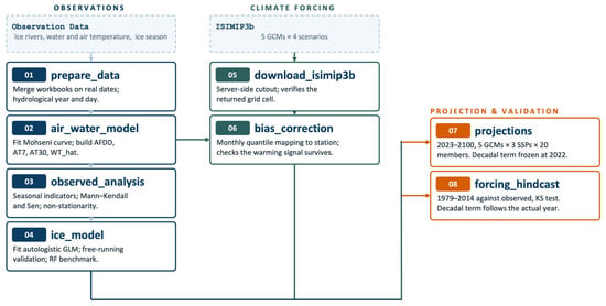
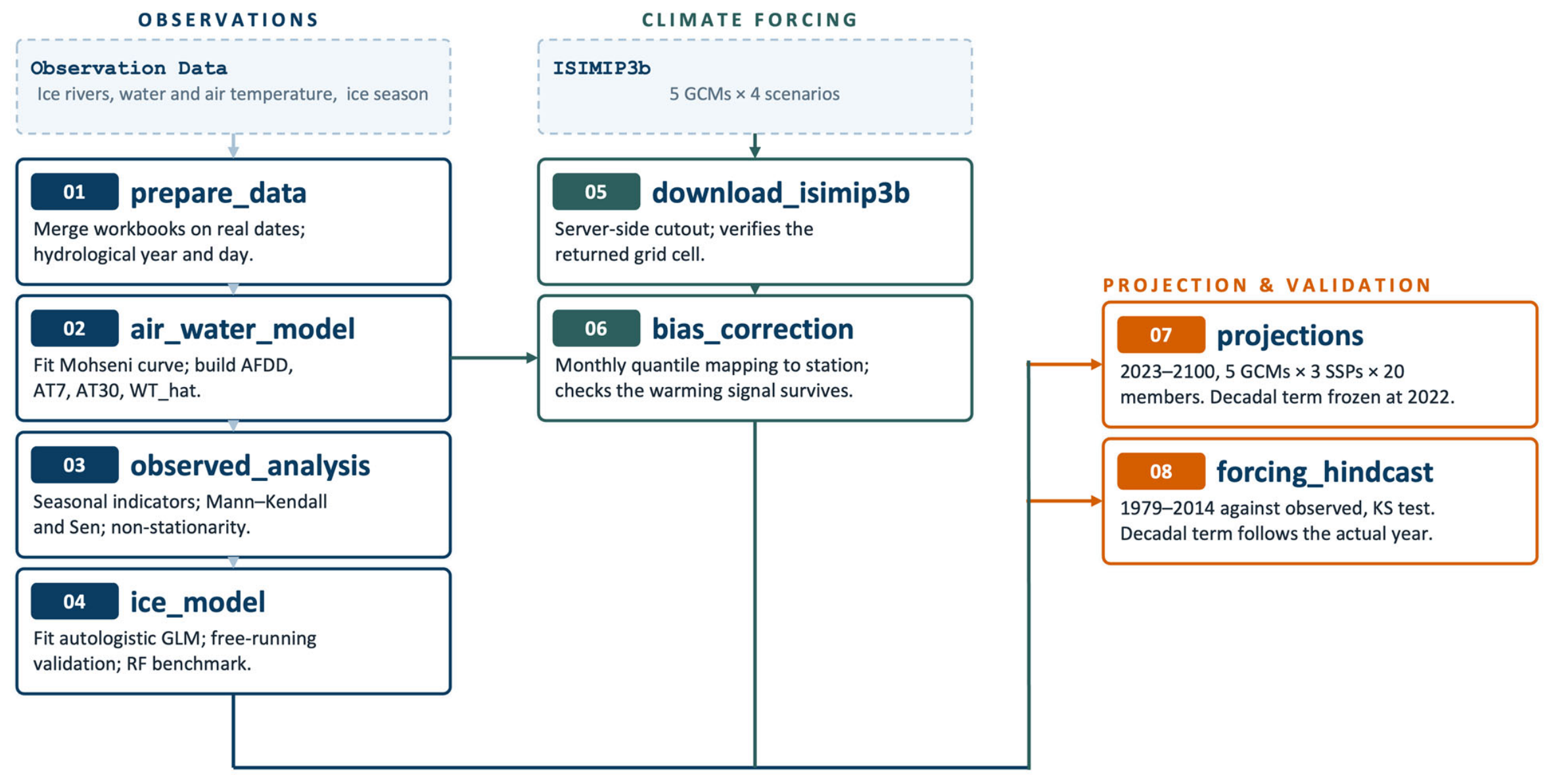
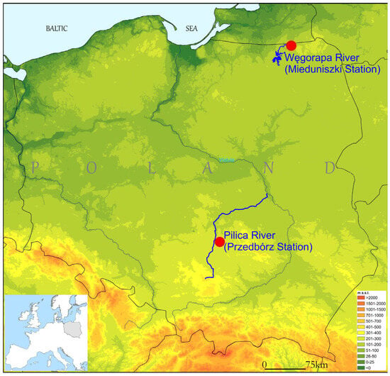
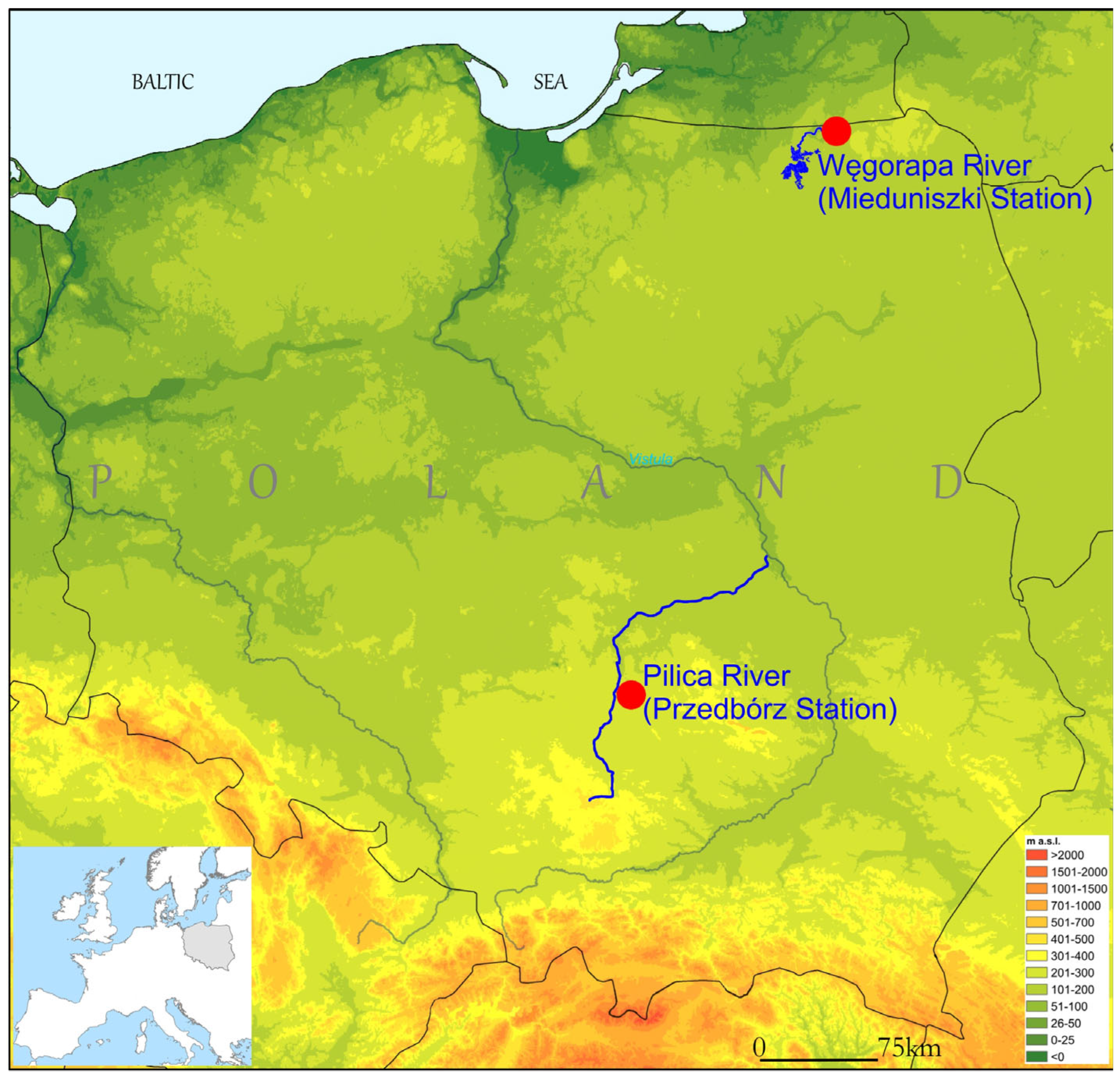
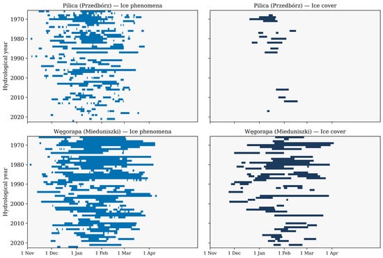
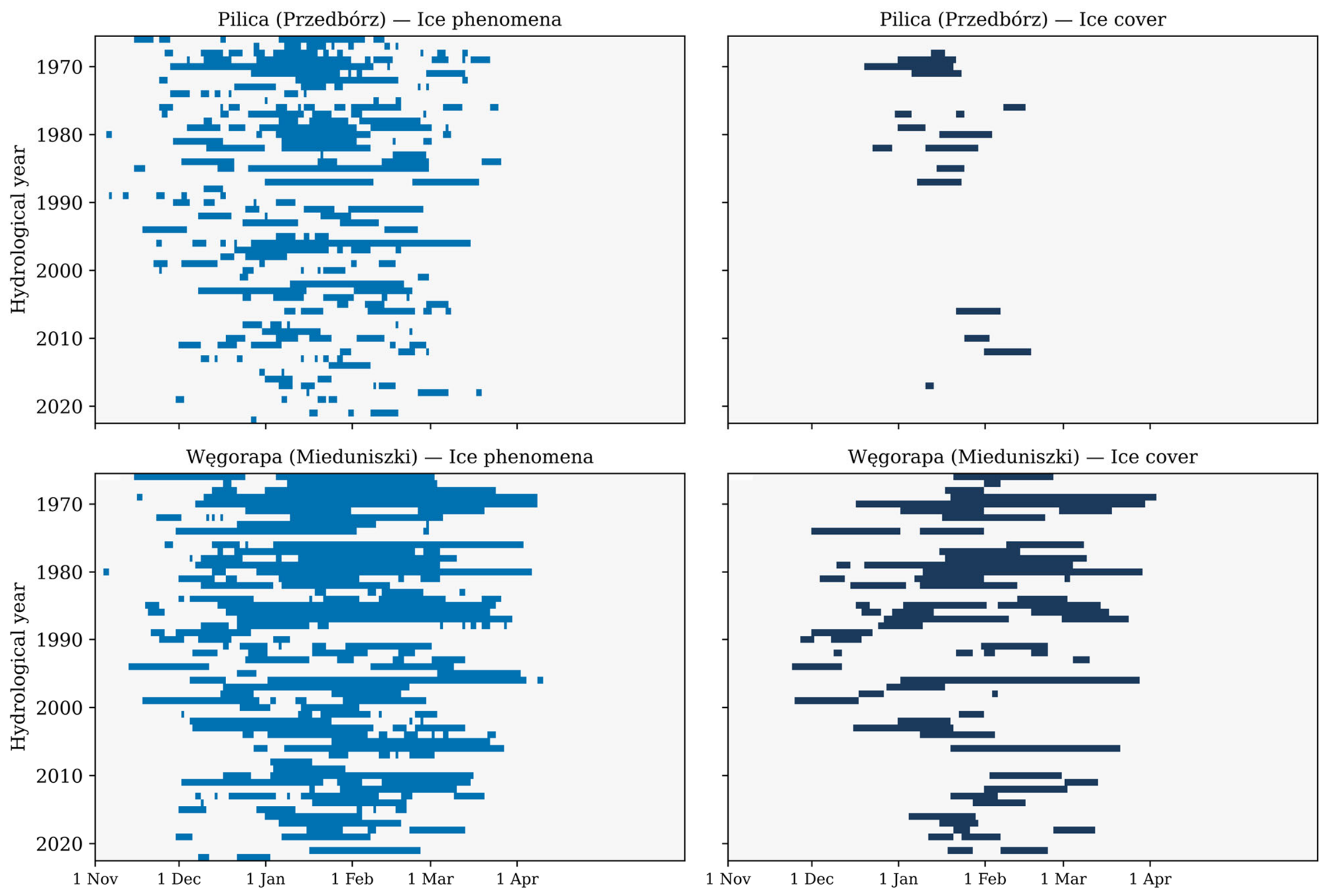
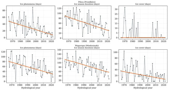
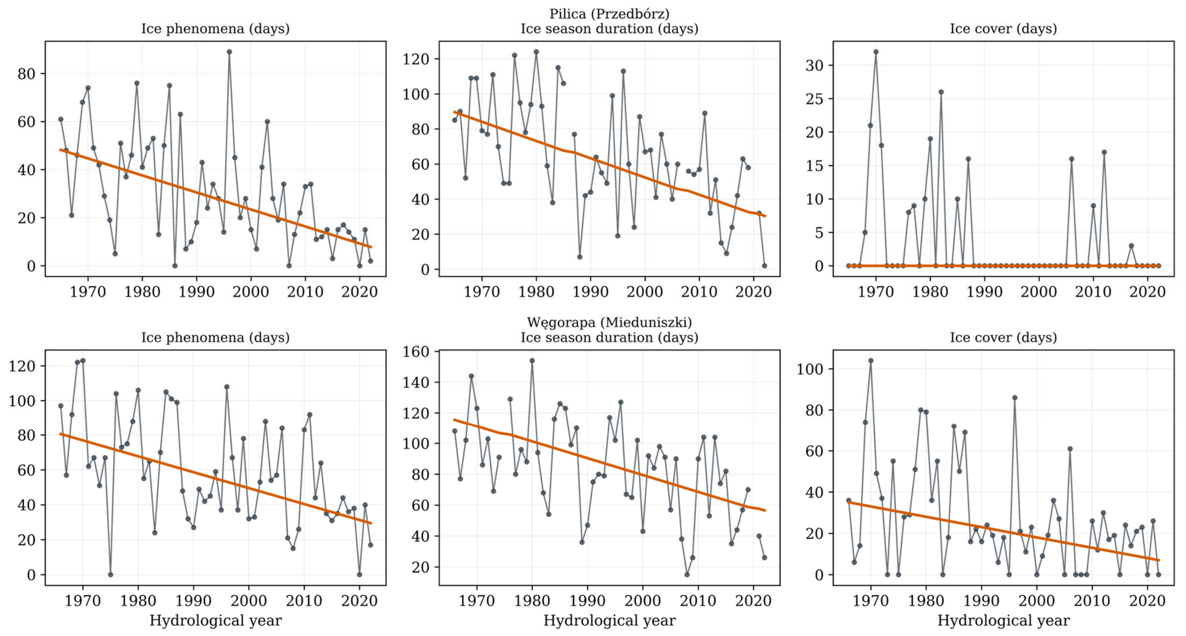
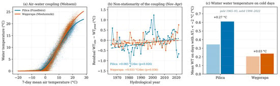
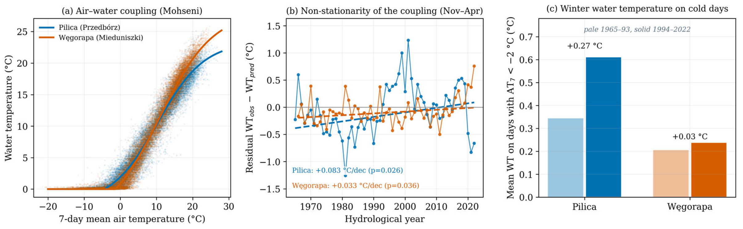
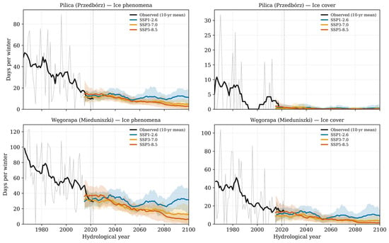
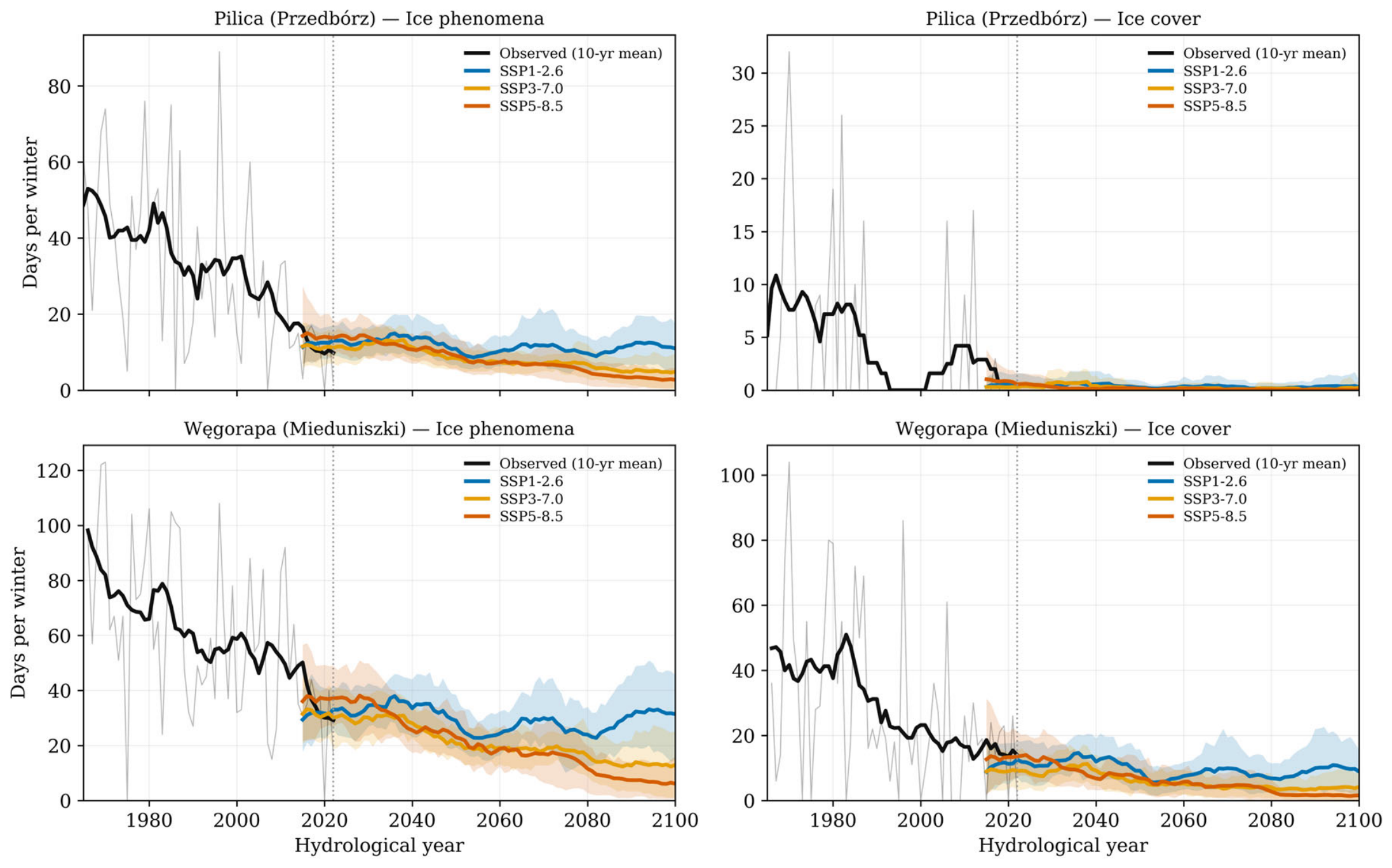
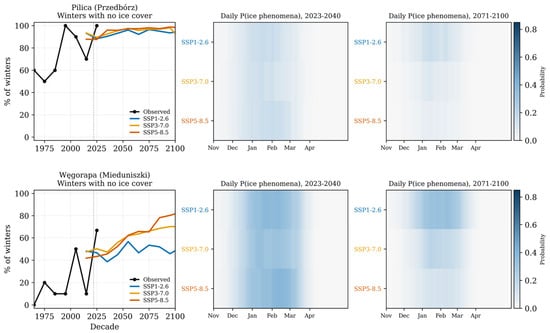
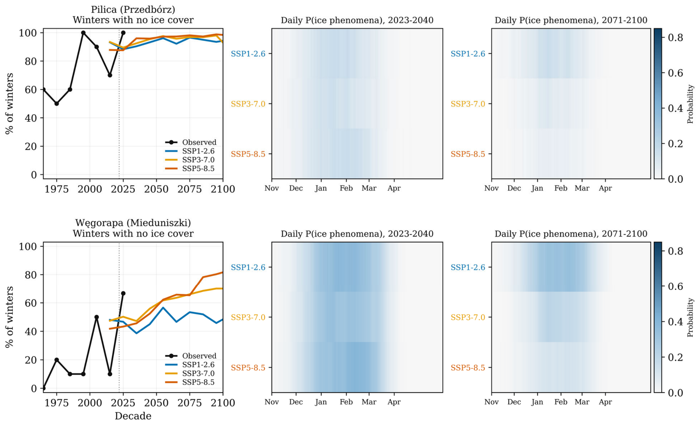

Disclaimer/Publisher’s Note: The statements, opinions and data contained in all publications are solely those of the individual author(s) and contributor(s) and not of MDPI and/or the editor(s). MDPI and/or the editor(s) disclaim responsibility for any injury to people or property resulting from any ideas, methods, instructions or products referred to in the content. |
© 2026 by the authors. Licensee MDPI, Basel, Switzerland. This article is an open access article distributed under the terms and conditions of the Creative Commons Attribution (CC BY) license.