


Abstract
Precise short-horizon solar-irradiance forecasting is essential for grid-tied inverter control and battery scheduling in arid climates, yet model performance in regions with frequent dust remains under-characterized. This study benchmarks six machine-learning models—Linear Regression, Support Vector Regression (SVR), Random Forest, XGBoost, Gradient Boosting, and Long Short-Term Memory (LSTM)—for 1-, 3-, and 6-h-ahead Global Horizontal Irradiance forecasting using 34,871 hourly records from Riyadh, Saudi Arabia (2013–2016). All models were tuned with temporal cross-validation and evaluated on an independent 2016 test set. Two feature tracks were evaluated: a full twenty-five-feature set and a three-feature set (hour_sin, hour_cos, GHI_lag_1) selected by recursive feature elimination with 100% bootstrap stability. A four-feature SVR adding doy_cos is the empirical optimum at 1- and 3-h horizons, achieving an RMSE of 65.43 and 77.16 W/m2 (R2 0.956 and 0.948, skill scores 61.5% and 82.8%). At 6 h, Gradient Boosting with the full 25-feature set is best (RMSE 78.99 W/m2). The three-feature LSTM achieves 98.25, 148.84, and 233.47 W/m2. Split-conformal prediction achieves nominal 90% coverage (89.56%, 90.30%, 89.65%) with CRPS of 25.94, 31.36, and 32.42 W/m2, and intervals 7–21% narrower than quantile regression. A matched-condition dust analysis shows no statistically significant difference between dusty and clean days at 1- and 3-h horizons, while at 6 h, dusty days are significantly easier to forecast (37% lower RMSE, 95% CI [−37.46, −11.04]). A reserve allocation simulation using the four-feature SVR shows 9.1% savings at 1 h, 3.6% at 3 h, and 2.4% at 6 h at 94.9% empirical coverage. Rolling-origin validation across two temporal windows confirms stability (SVR standard deviation ≤ 1.8 W/m2).
1. Introduction
1.1. The Challenge of Solar Forecasting for Grid Integration
This landscape of energy sources on a global level is experiencing profound changes due to the pressing need to address the problem of climate change and move towards sustainable energy systems. One of the energy solutions that has gained popularity during the last decade is the photovoltaic (PV) solar cells. The Kingdom of Saudi Arabia, in particular, has developed an ambitious plan of Vision 2030 aimed at the introduction of renewable energy sources, which has been motivated by the favorable conditions for harnessing solar power available in the country [1,2]. However, the incorporation of solar PVs into the modern power grid is associated with a number of difficulties inherent to the intermittency of solar irradiance [3].
Solar-irradiance forecasting has become one of the most important steps of PV implementation that has many functions [4,5]:
- Control of grid-tied inverters: To ensure efficient power delivery, voltage regulation, and reactive power support via the implementation of predictive control techniques that can account for fast irradiance variations [1,6].
- Scheduling of BESS: Optimization of the charging and discharging process for balancing supply and demand, lowering operating costs, and maximizing battery life span [7].
- Maintenance of power quality: Control of ramp rate, reduction of voltage fluctuations, and ensuring grid stability under variable generation [3,8].
- Economic dispatch: Reduction of operating costs, minimization of dependence on costly spinning reserve, and optimization of participation in day-ahead markets [9].
- Predictive maintenance: Prediction of inverter stress and degradation due to fast irradiance variations, prolonging inverter lifetime, and decreasing downtime [10].
Grid-tied inverters represent the critical interface between photovoltaic arrays and the utility grid that needs to cope with rapid irradiance variation for power quality and grid security purposes [1,8]. Fast irradiance variations that occur during cloudy periods and dust storms result in voltage violations, harmonics, and even the tripping of the inverter [7]. The probabilistic forecast allows the generation of information required for robust control of grid-tied inverters by implementing dynamic ramp-rate limits [11].
1.2. The Arid Climate Challenge
Arid and semi-arid zones that make up around 30% of the earth’s total land area have special difficulties in terms of solar forecast and photovoltaic systems operations [1,2]. The Kingdom of Saudi Arabia, located centrally on the Arabian Peninsula, exhibits such difficulties because of the following factors [6,12]:
- Dust occurrences: Dust storms and airborne dust particles are the most challenging conditions for solar forecasting in arid areas [7,12]. Such dust occurrences decrease surface irradiance by 20–80% in a few hours, having relatively fast occurrence times and making classical prediction models hard to be used [13]. Dust aerosols decrease irradiance in both direct and diffuse parts of solar radiation through the mechanisms of scattering and absorption, and the extent of their impact depends on dust particles distribution and composition [14]. Spring months in Saudi Arabia (March–June) feature the Shamal winds that transfer huge amounts of mineral dust from the Rub’ al Khali and Mesopotamian floodplain zones, making the forecast difficult on a seasonal basis [12,15].
- Temperature fluctuations: There are extreme daily and annual variations of temperature in arid climates; for instance, temperatures in summer in Riyadh can be above 45 °C. High temperatures decrease efficiency of PV modules (by 0.3–0.5% per degree above 25 °C), influencing the functioning of inverter power electronics and introducing additional nonlinearities into the forecast problem [6,16].
- Low humidity and aerosol dynamics: Low humidity in the atmosphere affects aerosol optical properties, transmittance in the atmosphere, and the production of secondary aerosols. Variations in aerosol optical depth on a daily and seasonal basis could affect irradiance attenuation up to 3–5-fold, requiring models that simulate both short- and long-term aerosol dynamics [13,14].
- Seasonal variation characteristics: The arid environment is characterized by distinct seasonal characteristics where high atmospheric load of aerosols leads to well-defined seasonality in terms of forecast difficulty [12]. In addition, the forecast error is found to be the highest during the spring months according to the study done [15].
Previous studies have assessed forecasting models for temperate climate environments thoroughly; however, there is limited knowledge regarding the model’s performance in arid regions [17]. Knowledge gaps include: (i) effects of dust occurrence on the performance of the forecasting models quantitatively, (ii) effectiveness of machine-learning algorithms for arid environment with dust occurrences frequently, (iii) seasonal variation of forecast performance with respect to dust climatology, and (iv) probabilistic uncertainty quantification for inverter control applications [17,18].
1.3. Related Work
1.3.1. Deterministic Forecasting Approaches
Solar-irradiance prediction techniques vary greatly, ranging from traditional statistical methods to machine learning and hybrid techniques [17,19].
The persistence method that assumes irradiance at time t + h will be equal to the irradiance at time t is the simplest method and can prove to be surprisingly efficient for extremely short forecast horizons in steady conditions [19]. Autoregressive integrated moving average models and exponential smoothing are widely applied for predicting solar irradiance [20]. The former considers temporal autocorrelation and seasonality but does not account for nonlinearity and dust storms [20]. Numerical Weather Prediction models, such as the Global Forecast System, can predict irradiance at coarse resolutions and are mainly used for day-ahead predictions [21]. Satellite predictions using geostationary satellites allow obtaining cloud-motion vectors and estimating irradiance [22]. Nonetheless, physical models cannot account for rapid changes characteristic of dust storms and local atmospheric conditions [17].
1.3.2. Machine-Learning Approaches
However, machine learning has become an appealing choice compared to physical models by allowing capturing complex non-linear interactions without physical parameterization [4,23,24].
Support Vector Regression (SVR) utilizing different kernels has been used for irradiance forecasting. SVR has shown excellent performance in capturing non-linear relations in small training datasets [25]. However, SVR suffers from poor performance in large-scale datasets and high dimensionality and difficult tuning of its parameters [26]. Random Forest, which trains a multitude of decision trees via bootstrap aggregation, has proven to be a robust method for irradiance forecasting [24]. Main advantages of Random Forest include capability to work well with non-linear relations, ability to rank features, avoid overfitting, and efficiency [27]. XGBoost, a gradient-boosting algorithm, building trees one-by-one with regularization, has shown outstanding performance in recent studies [28]. Gradient Boosting provides similar capabilities with slightly smaller computation costs [29]. Long Short-Term Memory (LSTM) neural networks developed specifically for sequence predictions have been widely used for time-series forecasting [30]. The LSTM’s capability to model long-term dependencies makes it well-suited for irradiance forecasting [31]. Hybrid approaches like CNN-LSTM and BiLSTM incorporating spatial features extraction with temporal models have shown state-of-the-art performance in some studies [32,33]. However, the deep-learning models require large training datasets, extensive hyperparameter tuning, and expensive computations providing insignificant improvement over ensembles [32].
The recent research has highlighted the importance of using hybrid methods, which can be designed on the basis of combining several algorithms to leverage their benefits [23]. For instance, combining K-Nearest Neighbors with Extreme Gradient Boosting has resulted in better results in the case of predicting Global Horizontal Irradiance with RMSE as low as 24.18% and R2 of 99.94% [34]. The VotingRegressor methods optimized through meta-learning, which can adjust the weight of base models, have shown remarkable decreases in RMSE and MAE with maintaining R2 [35]. Similarly, ensemble voting approaches that combine multiple base models have been shown to significantly reduce forecast errors and improve overall accuracy [36].
1.3.3. Probabilistic and Uncertainty Forecasting
Importance of probabilistic forecasting has been increasingly acknowledged since deterministic forecasts do not provide any information on how confident we are in our forecasts [11]. The idea of quantile regression has been applied to trees and Gradient-Boosting algorithms [21], which enables us to make prediction intervals for certain quantiles and consequently quantify uncertainty for every forecast [37]. Conformal prediction, being a distribution-free approach to uncertainty quantification, allows us to create confidence intervals that cover the true value with a guaranteed rate regardless of the probability distribution of the input data [38]. Furthermore, it is crucial to consider the broader impact of weather variability on solar-energy production forecasting when developing and deploying these probabilistic models [39,40].
1.3.4. Arid Climate and Dust-Impact Studies
Several studies have considered the radiative impact of dust aerosols on solar radiation using either satellite observation or radiative transfer models [13,15]. Papachristopoulou et al. assessed the impacts of dust on solar radiation in the Mediterranean Basin for 15 years, finding reductions in surface irradiance due to dust of 10–40% [13]. Kosmopoulos et al. utilized model simulations, satellite, and ground-based observations to assess the impact of dust on surface solar radiation [14].
In the Arabian Peninsula, Maghrabi studied the impact of dust storms on solar radiation data and found that dust storms can reduce GHI by 30–70%, while the diffuse fraction was significantly increased due to dust storms [12]. Alharbi et al. assessed a dust storm in Saudi Arabia and identified the synoptic patterns associated with the generation of dust storms [15]. Seasonal variability of dust events in the Arabian Peninsula has been characterized in prior work, with the maximum occurrence of dust events observed in springtime [12,15].
The academic research on solar forecasting in Saudi Arabia involved different machine-learning techniques. The works of Alkhaldi on the application of machine learning and artificial neural networks for solar-irradiance forecasting stressed the role of correlations between weather variables and issues with the integration into the grid [1]. Alhayd and Todeschini used the rich dataset of actual solar generation together with weather variables for predicting the supply of solar energy, determining important weather variables and comparing models’ performance [2]. AlSharabi et al. used Support Vector Machines and Gaussian Processes for long-range solar irradiation forecasting in Riyadh, considering factors like dust storms and weather variabilities [6]. Rashid et al. tested eight machine-learning models for direct solar radiation forecasting with an introduction of Trigonometric Cyclical Encoding increasing the explanatory power of temporal features by 49.26% for months and 53.30% for days [4].
On the other hand, there is a shortage of research that has attempted to quantify the effect of dust events on the accuracy of solar-irradiance forecasts across several prediction models and forecast horizons. It has been shown that the use of dust flags or aerosol optical depth as predictor variables could help improve forecast accuracy but not many benchmarks exist [18].
1.3.5. Saudi-Arabia-Specific Studies
Some research has been done to forecast solar energy in Saudi Arabia. An evaluation of Artificial Neural Network (ANN), Random Forest (RF), and Linear Regression models for solar-radiation forecasting in Riyadh showed that RF has the highest accuracy, i.e., 92.86%, while having the lowest RMSE of 10.3157 [25]. A forecast using autoregressive KNN-regression scheme for day ahead has been tested by Kamarianakis et al., and it was revealed that there is an improvement in terms of predictive accuracy in the range from 10% to 25% on average using 60 months of data from Thuwal, Saudi Arabia [26]. The best performing ANN model in predicting solar irradiation has been compared with other machine-learning techniques for the same task, and it was found that it has an RMSE of 25.92 W/m2 while outperforming the highly tuned Random Forest model [7]. Mishra et al. used extreme Gradient Boosting and Random Forest for better solar-radiation forecasting than traditional statistical approaches and it was found that their approach increased the accuracy by 39% [27]. Leholo et al. have developed KNN-XGB hybrid model for forecasting GHI with RMSE of 24.18% and R2 = 99.94% [34].
1.4. Gaps in Current Knowledge
Despite the existing large number of publications devoted to forecasting solar irradiance, there are still several significant problems:
- Poor benchmarking in arid locations: Most model benchmarking studies have been performed in temperate and tropical locations, while arid locations, which have special characteristics due to dust events, have not been represented sufficiently enough [17].
- Poor quantification of impact of dust: The quantitative dependence between dust occurrence and forecast error has not been investigated adequately enough [18].
- Underdevelopment of probabilistic uncertainty assessment for inverter control: Though probabilistic methods are available, the use of them for controlling grid-tied inverters considering ramp-rate limits and reserves has not been studied well enough [11].
- Poor consideration of seasonal changes: Seasonal forecast performance and its connection with dust seasons have not been investigated sufficiently enough [12].
- Lack of variety of models in benchmarking studies: Most benchmarking studies consider small numbers of models and do not perform the comparison of simple baselines, ensemble, and deep-learning models [5].
1.5. Contributions of This Study
Supplementary Tables S1 and S2 summarize the key findings from the existing literature and identify the critical research gaps that this study addresses, including the limited benchmarking in arid climates, insufficient quantification of dust impact on forecast accuracy, and the lack of probabilistic uncertainty assessment for inverter control applications [6,12,13,15,25]. This work provides novel findings to fill the aforementioned gaps:
- A benchmarking exercise of six machine-learning algorithms for hourly GHI prediction: Linear Regression, Random Forest, XGBoost, Gradient Boosting, Support Vector Regression, and LSTM with the addition of a simple persistence benchmark, using a four-year dataset recorded in Riyadh, Saudi Arabia.
- A matched-condition dust analysis controlling for hour-of-day and season, which finds no statistically significant difference in forecast error between dusty and clean days at any horizon.
- A creation of probability intervals based on quantile regression and conformal prediction and an evaluation of their coverage and width for practical inverter control purposes.
- A seasonal analysis of model performance and the investigation of the link between forecast accuracy and the dust seasonality of the Arabian Peninsula.
- Guidelines for model selection, considering accuracy and computation needs, for practical inverter control and BESS scheduling in arid climate zones.
- Feature importance analysis and an estimation of the contribution of dust-related features to prediction.
1.6. Paper Structure
The structure of this paper is as follows. Section 2 describes study case, dataset, feature engineering, forecasting methods, evaluation procedure, and uncertainty quantification approaches. Section 3 describes results of experiments. Section 4 gives discussion on implications of research in terms of inverter control, BESS scheduling, and power converter design and mentions limitations and directions for further research. Section 5 provides conclusions.
2. Data and Methodology
2.1. Study Site and Dataset
The solar radiation and meteorological data used in this study were obtained from the Renewable Resource Monitoring and Mapping (RRMM) Program, conducted by the King Abdullah City for Atomic and Renewable Energy (K.A.CARE). The dataset covers a four-year period (2013–2016) from the Riyadh measurement station (24.52958° N, 46.43635° E; “K.A.CARE City T2”), Saudi Arabia [41]. The study site is based at the Center for Riyadh which has a hot arid desert climate (BWh Köppen classification), featuring very low annual rainfall (<100 mm), extremely high summer temperatures above 45 °C, and dusty conditions due to frequent dust storms especially in spring and early summer seasons [6,12]. It is based in an urban area with no shading, guaranteeing clear measurement of solar radiation all year round. This site represents the larger central Arabian Peninsula region which is currently undergoing fast deployment of solar-energy technologies as per Saudi Vision 2030 [1,2].
The dataset consists of precise measurements of the solar radiation components and other meteorological parameters measured at a 1-min resolution followed by aggregation into one-hour average values. Solar-radiation data was collected using Kipp and Zonen CMP21 pyranometers for GHI and DHI and Kipp and Zonen CHP1 pyrheliometer for DNI [12]. Air temperature, humidity, atmospheric pressure, wind speed, and direction were measured using Campbell Scientific instruments. All instruments were calibrated annually as per ISO 9060 standards; the pyranometers were ventilated in order to reduce thermal offset errors and the shadow ring used in measuring DHI was weekly adjusted based on the sun’s declination.
The source file contains 34,871 hourly records with valid GHI, spanning 2 January 2013 to 31 December 2016—169 h fewer than the theoretical 35,040 hourly slots, reflecting documented station downtime for calibration, maintenance, and transmission gaps. Section Data Pipeline and Per-Horizon Sample Flow provides the complete sample flow.
Figure 1 presents a schematic view of the whole methodology pipeline used throughout the work. The pipeline includes all processes of collecting, processing, preparing data, building models, making forecasts, and their assessment. This flowchart represents the entire experimental pipeline used in this study. This process starts with the step of data collection and data quality checking (Section 2.1 and Section 2.2), which is then followed by the process of feature engineering (Section 2.3), in which the construction of temporal, lagged, meteorological, and dust-event features is done. After that, the steps of model training and forecasting (Section 2.4 and Section 2.5) are conducted using six different machine-learning models for three different forecast horizons, which are 1 h, 3 h, and 6 h. The next step is probabilistic forecasting (Section 2.6), which uses quantile regression and conformal prediction.
Figure 1.
Methodology workflow for solar-irradiance forecasting.
2.2. Data Quality Control
Physical range checks required GHI ≥ 0, DHI ≥ 0, DNI ≥ 0, GHI ≤ 1.2 × I0, zenith angle ∈ [0°, 180°], temperature ∈ [−10 °C, 60 °C], relative humidity ∈ [0%, 100%], and pressure ∈ [800 hPa, 1100 hPa]. Physical consistency checks required DHI ≤ GHI and DNI ≤ GHI/cos(θz) for θz < 80°. The clearness index Kt = GHI/I0 and diffuse fraction Kd = DHI/GHI were constrained to [0, 1] [27].
- Timestamp parsing. The source file contains two date formats: d/m/yyyy h:mm (no seconds, single-digit month and day) and dd/mm/yyyy hh:mm:ss (with seconds). A strict format-agnostic parser using format = ‘mixed’, dayfirst = True was applied, followed by removal of any rows with unparseable dates (none in the final dataset) and deduplication of repeated timestamps (keep-first).
- Zenith recovery. The station’s sun tracker provides a Zenith Angle column that is 45.4% missing (15,821 of 34,871 records) due to tracker downtime. Because zenith is deterministically recoverable from the timestamp and station coordinates, we recomputed it astronomically for the missing rows:
cos(θz) = sin(φ)·sin(δ) + cos(φ)·cos(δ)·cos(H)
Data Pipeline and Per-Horizon Sample Flow
To ensure full reproducibility and to allow verification of the temporal alignment of predictors and targets, we explicitly track sample reduction through each stage of the data pipeline. Table 1 presents the sample counts at each processing stage.
Table 1.
Data-pipeline sample counts.
2.3. Feature Engineering
2.3.1. Temporal Features
Solar-irradiance forecasting entails proper modeling of the cyclic deterministic patterns associated with solar energy [7,19]. In order to account for these cycles, we developed a suite of temporal features. Hour of the day was modeled through sine and cosine transformations due to the cyclicality of time as follows:
Similarly, the day of year was transformed using:
for capturing the seasonal changes in the solar declination and the duration of the day [7]. Some other temporal features were months (1–12), weekday (0–6), and categorical season feature (Winter, Spring, Summer, Autumn) based on the value of the month.
The above transformations are crucial because some machine-learning algorithms do not natively account for cyclical data [19]. Sine–cosine transformation guarantees that hours near midnight (23:00 and 01:00, for example) will be closed in the feature space without any artificial jumps due to integer hour representation.
2.3.2. Lagged Features
GHI lagged values at 1, 2, 3, and 6 h were computed on the full chronological series—before daytime filtering—so that each lag corresponds to exactly the stated elapsed time in real hours, including across day boundaries. This is the key methodological point: the lag features at the first hour of a calendar day reflect the last available nighttime record rather than the last daytime record of the previous day, which is physically correct. Lag verification on a random sample of 100 daytime rows confirms that GHI_lag_1 matches the measured GHI exactly one hour earlier in 100/100 cases. Lagged time windows were chosen with an emphasis on both short-time (1 to 3 h) and medium-time (6-h) lags, which might provide predictive power for forecasting [5]. The use of lagged features is especially essential in arid regions, where high variability of irradiation occurs due to clouds of dust events and their persistence serves as a good predictor [12].
2.3.3. Meteorological Features
The following meteorological parameters have been used as predictors to take into consideration the atmospheric effects on solar irradiance [1,16]. They include temperature, relative humidity, wind speed, and barometric pressure. These parameters are measured when predicting the solar irradiance (t). The temperature impacts the PV cells’ efficiency and atmospheric transmissivity, while the relative humidity affects aerosols and clouds [14]. The wind speed is an essential predictor for the arid area as it causes dust emissions [12]. The pressure parameter represents the synoptic weather pattern.
For the 1-h and 3-h forecasts, the lagged meteorological parameters (temperature, RH, wind speed at t − 1, t − 2) have also been used as predictors [2].
2.3.4. Dust-Event Features
One of the innovations of this study is the inclusion of dust-event information explicitly as a feature [12,15]. Based on the dust-event definition established in the prior study, we developed a binary dust flag, which denotes whether the wind speed exceeds the threshold (85th percentile) value of 5.42 m/s along with wind blowing from the north-northwest direction (315–45°) [12]. In terms of forecasting horizons, the dust flag was calculated based on the current wind state assuming that there will be enough persistency in wind conditions for dust-event continuation.
Additionally, the moving averages and standard deviations of wind speed within the past 3, 6, and 12 h were utilized to take into account the intensity and persistency of the wind conditions, which might denote either development or dissipation of the dust event [12,36]. The use of such features makes it possible for the model to anticipate the impact of dust event on attenuation although wind speed might not be a reliable indicator itself.
The pipeline of feature engineering procedure is represented in Figure 2. It shows how four kinds of features–temporal, lagged, meteorological, and dust-event features–are generated and combined in the resulting feature set consisting of 25 predictors. Figure 2 shows the development of all input features based on raw hourly data. The temporal features contain information about the diurnal and seasonal cycle using sine and cosine transformations (hour_sin, hour_cos, doy_sin, doy_cos, month, weekday, season). The lagged features incorporate the temporal autocorrelation of GHI at lag 1, 2, 3, and 6 h (GHI_lag_1 to GHI_lag_6). The meteorological features consist of current and lagged temperature, relative humidity, wind speed, and atmospheric pressure. The dust events features contain a binary dust-event flag, which considers wind speed ≥ 5.42 m/s and direction 315–45°, and wind speed mean and standard deviation over 3, 6, and 12-h rolling periods.
Figure 2.
Feature-engineering pipeline for solar-irradiance forecasting.
2.3.5. Target Construction and Temporal Alignment
Forecast targets were constructed on the full chronological series:
For each horizon , the per-horizon dataset was obtained by filtering the full series to rows satisfying:
- and (current row is daytime);
- is not and (target is a valid daytime irradiance);
- All lag features are present.
Daytime filtering therefore happens after target construction, not before. This preserves the correct temporal meaning of both the lag features and the target values at day boundaries. The residual overnight gap in the source data is handled by the filter: rows with nighttime targets are simply excluded.
Feature scaling fits on training data only. Validation subsets (last 15% of training) are used for LSTM early stopping and for conformal calibration. The 2016 test year is never used for model selection, hyperparameter tuning, or feature selection.
2.4. Forecasting Models
A total of six different machine-learning models ranging from simple linear ones to more complex ensemble and deep-learning algorithms were analyzed [4,17]. Such an approach permits the benchmarking process which enables us to achieve the best compromise between accuracy, computational effort, and model interpretability [8].
2.4.1. Persistence Model (Baseline)
Three persistence-based baselines are included to provide a reference for forecast skill. The simple persistence model assumes that the irradiance at the forecast horizon equals the current irradiance:
where is the predicted GHI at time , is the measured GHI at time , and is the forecast horizon.
The clear-sky persistence model scales the climatological clear-sky irradiance at the target time by the current clearness index:
where is the clear-sky reference GHI for the hour of day corresponding to time . In this study, is estimated as the 95th percentile of measured GHI at each hour of day in the training set (2013–2015), which provides a robust and data-driven clear-sky proxy without requiring radiative-transfer modeling.
The smart persistence model extrapolates the recent trend in GHI using the lag- observation:
where is the measured GHI hours before time . This trend-extrapolation baseline is particularly relevant for arid climates where the diurnal cycle produces a strong, predictable irradiance ramp.
All three baselines are evaluated on the same test set (2016) and against the same metrics (RMSE, MAE, R2, MAPE, skill score) as the machine-learning models, ensuring a consistent comparison framework.
2.4.2. Linear Regression
Linear regression acts as a basic machine-learning benchmark where the connection between the features and the target is established by modeling a linear relationship between the variables [25]. However, even being simple, linear regression can work well if there is an approximately linear dependence between the features and irradiance values, giving coefficients that show how important each variable is [17]. It was used through the “sklearn.linear_model.LinearRegression” class with default settings.
2.4.3. Random Forest
Random Forest is an ensemble learning technique that builds a forest of decision trees during training and gives the average predictions of the individual trees [9,18]. It avoids overfitting and enhances the generalization capacity compared to the decision tree [24]. The reason why Random Forest is a good fit for solar-irradiance prediction is that it allows modeling nonlinear dependencies and interactions of variables without knowing their functions and is resistant to outliers and multicollinearity [10,29]. Hyperparameters were tuned per horizon using the TimeSeriesSplit protocol of Section 2.4.8. The selected values are in Table 2.
Table 2.
Hyperparameter search spaces and final selected values.
2.4.4. XGBoost
XGBoost (Extreme Gradient Boosting) is the scalable implementation of the Gradient-Boosting algorithm that has turned out to be the state-of-the-art tool for structured data regression [28]. This approach is based on the construction of ensembles of decision trees in sequence, where each successive tree corrects mistakes of its previous ones [4]. There are some benefits associated with the use of XGBoost such as regularization to avoid overfitting, missing values support, and tree pruning [29]. Hyperparameters were tuned per horizon using the TimeSeriesSplit protocol of Section 2.4.8. The selected values are in Table 2.
2.4.5. Gradient Boosting
Another variant of the Gradient-Boosting algorithm (sklearn version) is a Gradient Boosting algorithm, that trains trees one after the other, minimizing the loss function [29]. Although very much like XGBoost, the sklearn version of the algorithm is easier to use [9]. This model was built using “sklearn.ensemble.GradientBoostingRegressor” [24]. Hyperparameters were tuned per horizon using the TimeSeriesSplit protocol of Section 2.4.8. The selected values are in Table 2.
2.4.6. Support Vector Regression
SVR (Support Vector Regression) is a kernel method that projects the input variables to a higher-dimensional space where linear regression is applied [25]. SVR can model highly nonlinear mappings using a suitable kernel [10]. The SVR algorithm was built using “sklearn.svm.SVR” with an RBF kernel [25]. The hyperparameters (C, gamma, epsilon) were tuned using the TimeSeriesSplit protocol of Section 2.4.8. The final configuration was C = 100, gamma = “scale”, epsilon = 0.1 at all horizons.
2.4.7. Long Short-Term Memory (LSTM) Network
An LSTM network is a kind of RNN architecture, tailored to learn long-term dependencies from sequential data [30,31]. LSTM architectures are distinguished from feed-forward models due to maintaining internal state capable of memorizing information over time and, therefore, useful for time-series prediction tasks [32]. A basic LSTM network with two hidden layers having sixty-four units each and a dense layer was used. The training was done using the Adam optimizer with the learning rate of 0.001 and mean squared error loss function. Dropout layers (rate = 0.2) were added after each LSTM layer to avoid overfitting [30].
Two variations of the LSTM model were considered: (1) full-feature LSTM including all 25 features, but convergence properties were poor for this configuration because of the small dataset size and high dimensionality; (2) reduced-feature LSTM considering only the top-three features (hour_sin, hour_cos, GHI_lag_1) and showing excellent results. Then, the three-feature LSTM was compared to all other models using the same set of three features.
The LSTM was implemented in TensorFlow 2.21.0 with the following specifications:
- Input tensor construction: Sliding windows of length L = 24 h with three features (hour_sin, hour_cos, GHI_lag_1), each window paired with the target at t + h.
- Sequence length: L = 24 h, selected from autocorrelation analysis (ACF drops below 0.5 at 24 h).
- Architecture: two stacked LSTM layers with 64 units each, dropout rate 0.2, followed by a Dense(1) output layer.
- Weight initialization: Glorot uniform, random seed 42.
- Optimizer: Adam (learning rate 0.001).
- Loss function: Mean Squared Error (MSE).
- Batch size: 64.
- Epochs: Maximum 200 with early stopping (patience = 15) on validation loss.
- Validation set: Last 15% of the training period (late 2015).
- Feature scaling: StandardScaler fit on training data only.
A variant using all 25 features was also trained but failed to converge (RMSE ≈ 600 W/m2), which we attribute to the high feature-to-sample ratio (~25 features × 4722 training hours). This variant is excluded from the main results.
The three-feature LSTM (hour_sin, hour_cos, GHI_lag_1) achieves competitive performance against full-feature models, as reported in Section 3.2.
A minimal LSTM architecture was used as a sequence-model baseline: two stacked LSTM layers of 64 units each, dropout 0.2 after each, dense output of 1 unit. Training: Adam optimizer with learning rate 0.001, MSE loss, batch size 64, max 200 epochs with early stopping (patience 10) on the validation loss. Weight initialization: Glorot uniform with random seed 42.
Input sequences of length 24 h were built from the full chronological series (hour_sin, hour_cos, GHI_lag_1 at each step), so that nighttime hours are included in the lookback window. The prediction target is the daytime GHI at t + h. Sequences whose target fell outside the daytime set (or whose feature window contained NaN) were excluded. This construction is physically correct: the model sees the true preceding 24 h, not a compressed daytime sequence.
LSTM test samples were compared against the tabular models on the same test timestamps (verified by index intersection). LSTM RMSE values reported in Section 3.2 therefore use only the subset of test rows for which a full sequence and a valid target were both available. Section 4.5 notes the small difference in test sizes as a limitation.
2.4.8. Hyperparameter Optimization Protocol
All non-linear models (SVR, RF, XGBoost, GB) were tuned with TimeSeriesSplit(n_splits = 3) on the training years (2013–2015). For each model, 50 parameter combinations were sampled from the search space in Table 2, and the configuration minimizing mean cross-validation RMSE was selected. Linear Regression has no hyperparameters. The LSTM was not grid-searched (computationally prohibitive), and its architecture was fixed as documented in Section 2.4.7.
2.5. Forecasting Setup
2.5.1. Forecast Horizons
We tested all the models in three forecast horizons: 1 h, 3 h, and 6 h ahead [4,5]. We chose these forecast horizons because they meet the requirements of operational planning of grid-connected inverters and BESS [1]. Forecasting in the 1-h-ahead horizon helps to control the inverter ramp rate and power dispatch. The 3-h-ahead horizon allows for short-term scheduling and reserve management. The 6-h-ahead horizon can be used for day-ahead scheduling and optimization of battery energy storage [17].
2.5.2. Features Scaling
In case of Linear Regression, SVR and LSTM, features were scaled to zero mean and unit variance using “sklearn.preprocessing.StandardScaler” [27]. The parameters of scaling were fitted on the training set and then applied to both training and test sets in order not to violate the data independence [3]. Tree-based methods (Random Forest, XGBoost, Gradient Boosting) are not affected by the scale of features and were trained on the original values of features [22].
2.5.3. Data-Use Summary
Because the correctness of the reported results depends on strict separation between model-selection data and final-evaluation data, Table 3 documents which data partition was used at each step. Every decision about models, hyperparameters, feature subsets, and calibration was made using only 2013–2015 training data; the 2016 test year was reserved for final evaluation and was never used to make or revise any such decision.
Table 3.
Data use per training and evaluation step.
2.6. Probabilistic Forecasting Methods
A point forecast gives an estimate of the expected value of the variable to be forecasted but does not provide information about its uncertainty [11,38]. When considering the control of grid connected inverters and BESS scheduling, knowledge of the uncertainty of the forecast is necessary [21]. Therefore, we have developed two probabilistic forecasting methods.
2.6.1. Quantile Regression
The quantile regression method can predict the conditional quantiles of the distribution of the target variable and thus gives information on its uncertainty [36]. Quantile regression has been implemented using “sklearn.ensemble.GradientBoostingRegressor” model with the loss = “quantile” option, enabling the training of the model for the estimation of quantiles [38]. We have calculated the 5th, 25th, 50th (median), 75th, and 95th percentiles. This way we get 90% and 50% prediction intervals. The 90% prediction interval (5th–95th percentile) gives the bounds where the true irradiance is expected to lie with 90% certainty, whereas the 50% interval gives a narrower region.
2.6.2. Split-Conformal Prediction
We implement split-conformal prediction with a held-out calibration set to produce prediction intervals with finite-sample coverage guarantees [38,39].
- Step 1—Data split. The training data (2013–2015) is further split chronologically into:
- A proper training set containing the first 85% of the training period
- A calibration set containing the last 15% of the training period (late 2015)
- The test set (2016) is never used during calibration.
- Step 2—Base-model training. The base model—SVR, selected as the best-performing point forecast model—is trained on the proper training set only.
- Step 3—Non-conformity scores. For each sample in the calibration set, the absolute residual is computed:where is the measured GHI and is the SVR prediction.
- Step 4—Conformal quantile. The conformal quantile is computed as the quantile of the calibration residuals:where for a 90% target coverage level, and denotes the ceiling function.
- Step 5—Prediction-interval construction. For each test sample, the 90% prediction interval is constructed as:
- Coverage guarantee. Under the exchangeability assumption, the conformal interval satisfies Equation 10. Here the assumption is only approximate because the calibration set is drawn from late 2015 while the test set is the full year 2016. We report the empirical coverage on the 2016 test set in Section 3.10 and discuss the residual deviation in Section 4.5.In practice, the achieved coverage on the 2016 test set was 89.0%, 85.9%, and 84.4% for 1 h, 3 h, and 6 h horizons respectively (see Section 3.9 for discussion of residual under-coverage at longer horizons).
- Computational simplicity. Unlike quantile regression, split-conformal prediction requires only a single base model fit and one pass over the calibration set—making it computationally inexpensive and readily deployable in operational systems.
2.7. Evaluation Metrics
A range of metrics were used to measure both the point and probabilistic forecast accuracy [8,21].
2.7.1. Point Forecast Metrics
Root Mean Square Error (RMSE):
RMSE penalizes large errors and is sensitive to outliers, making it suitable for evaluating forecasting models where large errors have significant operational consequences [5,26].
Mean Absolute Error (MAE):
MAE provides an intuitive measure of average error magnitude and is less sensitive to outliers than RMSE [10,25].
Mean Absolute Percentage Error (MAPE):
MAPE expresses errors as a percentage of the observed value, providing a scale-independent measure of relative accuracy [4].
Skill Score:
The skill score quantifies the improvement of the model over the persistence baseline, with positive values indicating superior performance and 100% indicating perfect forecasting [5,26].
2.7.2. Probabilistic Forecast Metrics
Prediction Interval Coverage Probability (PICP):
For a 90% prediction interval, PICP should ideally be 0.90 [11,38].
Prediction Interval Normalized Average Width (PINAW):
where R is the range of the target variable. PINAW refers to the mean width of the prediction interval scaled by the range [21]. The narrower the prediction intervals, the more accurate the predictions will be.
Continuous Ranked Probability Score (CRPS):
CRPS is a proper scoring rule in the sense that it takes into account the entire distribution and therefore punishes overconfidence and underconfidence [21]. Small values of CRPS show good predictions.
2.8. Dust-Aware Analysis
To quantify the impact of dust events on forecast accuracy and to address the confounding effects of time-of-day, season, and irradiance magnitude, we perform three complementary analyses: a binary dust-day classification, a matched-condition comparison, and a transition-event analysis.
2.8.1. Dust-Day Classification
Following prior work on dust events in the central Arabian Peninsula [12,15], a binary dust flag is constructed from wind measurements:
where is the measured wind speed at time , is the 85th percentile of wind speed in the training set (equal to 5.42 m/s), and is the wind direction. The direction range corresponds to the Shamal wind sector, which is the dominant dust-transport pathway in the Arabian Peninsula [12,15].
Test samples are partitioned into dusty (dust_flag = 1) and clean (dust_flag = 0) subsets, and RMSE, MAE, and their relative differences are computed for each subset.
2.8.2. Matched-Condition Analysis
The binary dust flag alone cannot distinguish the effect of dust from confounding by time-of-day and season, since dust events in Riyadh occur predominantly in the spring and afternoon periods [12,15]. To isolate the dust effect, we perform a stratified matched comparison:
- Step 1—Stratification. Stratification used 5-h-of-day bins (6–8, 9–10, 11–12, 13–14, 15–17) × 4-month bins (DJF, MAM, JJA, SON) = 20 possible strata. Strata with fewer than three dusty or three clean samples were excluded; the number of non-empty strata used at each horizon (17, 15, 10 at 1, 3, 6 h) is reported in Section 3.5. The stratum identifier is:
- Step 2—Within-stratum matching. Within each stratum , dusty and clean samples are matched by taking the smaller of the two group sizes. This ensures that dusty and clean samples are drawn from identical hour-of-day and seasonal conditions.
- Step 3—Bootstrap confidence intervals. The difference in RMSE between matched dusty and clean samples is computed for each stratum, and 500 bootstrap resamples are used to estimate the 95% confidence interval on the mean difference:
A confidence interval that crosses zero indicates no statistically significant difference.
2.8.3. Dust Transition-Event Analysis
To characterize the forecast difficulty at the onset and end of dust events—which is often the operational bottleneck—we identify transitions in the dust flag series:
RMSE is computed over -h windows centered on each transition and compared to RMSE in stable dusty and stable clean periods. This identifies whether forecast degradation is associated with dust presence itself or with the transitions between atmospheric states.
2.8.4. Feature Importance and Dust-Flag Contribution
Feature importance is computed using three complementary methods:
- Linear Regression coefficients—providing linear sensitivity to each predictor [17].
- Random Forest impurity-based importance—capturing non-linear feature contributions [24].
- XGBoost gain-based importance—measuring the average gain achieved by splits on each feature [28].
Additionally, Recursive Feature Elimination (RFE) with 50 bootstrap iterations on the training set is used to assess the stability of feature selection, independent of any single importance metric. The dust flag’s rank in each importance ranking is analyzed to determine whether it adds predictive value beyond the top features identified by RFE.
2.9. Implementation Details
All analyses were implemented in Python 3.13 using the following libraries:
- scikit-learn 1.8.0—Linear Regression, SVR, Random Forest, Gradient Boosting, StandardScaler, TimeSeriesSplit, RandomizedSearchCV, RFE, and evaluation metrics [9,24].
- XGBoost 3.3.0—gradient-boosted tree implementation [28].
- TensorFlow 2.21.0—LSTM neural network implementation [30].
- NumPy (version 2.5.1) and pandas (version 3.0.3)—data manipulation and numerical computation.
- Matplotlib (version 3.10.7) and Seaborn (version 0.13.2)—figure generation.
Model training and hyperparameter optimization were performed on a workstation with 16 GB RAM and an Intel Core i7 processor. Training times ranged from seconds (Linear Regression) to minutes (LSTM), with tree-based ensembles requiring intermediate computational effort.
Code structure, hyperparameter search logs, random seeds, and configuration files are provided as Supplementary Material to ensure full reproducibility. All random seeds are fixed at 42 unless otherwise noted, and each experiment is repeated three times with seeds {42, 123, 456} to assess run-to-run variability.
3. Results
This section reports the benchmark in three tracks. Track A evaluates six machine-learning models on the 25-feature set. Track B evaluates the same models plus an LSTM on the three-feature set. Section 3.3 reports the canonical four-feature SVR identified by ablation as the empirical optimum at short horizons. All results use the temporal split of Section Data Pipeline and Per-Horizon Sample Flow, with 12,036/9921/6665 training rows and 4034/3330/2232 test rows at 1-, 3-, and 6-h horizons.
3.1. Track A: Full-Feature Benchmark (25 Features)
Table 4 reports the performance of all six models and three persistence baselines on the 25-feature set. Figure 3a compares the RMSE across models and horizons on a log scale.
Table 4.
Track A—Full-feature (25) benchmark.
Figure 3.
Track A RMSE comparison across models and horizons (log scale) (a), Track B RMSE comparison across models and horizons (b).
On the full 25-feature set, the tree and kernel models cluster tightly at 1 h: SVR is best (66.57 W/m2), followed by XGBoost (67.36), Random Forest (70.98), and Gradient Boosting (71.75). Linear Regression is fifth (76.27). At 3-h horizons the ranking compresses further, with Gradient Boosting (80.05), SVR (80.06), and XGBoost (80.31) separated by less than 0.3 W/m2. At 6 h, Gradient Boosting leads (78.99) followed by Random Forest (79.95). Linear Regression is consistently last among the ML models, confirming that the predictor–target relation is not purely linear.
The four tree and kernel models all achieve positive R2 at every horizon and monotonically degrade with horizon: 66.57 → 80.05 → 78.99 for SVR, and similar patterns for the others. This is the expected behavior.
Smart persistence exceeds simple persistence at 1 h (99.66 vs. 170.15 W/m2) but degrades sharply at 3 h and 6 h, becoming worse than simple persistence. This is expected: trend extrapolation helps over one hour, but small errors compound over longer horizons.
3.2. Track B: Reduced-Feature Benchmark (Three Features)
Table 5 reports the performance on the three-feature set (hour_sin, hour_cos, GHI_lag_1). Figure 3b shows the same results graphically.
Table 5.
Track B—three-feature benchmark (hour_sin, hour_cos, GHI_lag_1).
On the three-feature set, SVR is best at 1 h (66.36 W/m2) and 3 h (78.72 W/m2), while Random Forest leads at 6 h (81.08 W/m2). The top three models at 1 h—SVR (66.36), Random Forest (66.69)—are within 0.4 W/m2 of each other; XGBoost (81.75) and Gradient Boosting (199.09) degrade sharply when restricted to three features. This is a well-known weakness of shallow boosted trees under heavy feature reduction: with a max_depth of three (the tuned optimum for the 25-feature set), both GB and XGBoost can represent at most eight leaves per tree, which is insufficient to capture the smooth diurnal structure from only three inputs. Random Forest, with a tuned max_depth of 10, is more flexible and performs as expected.
The three-feature LSTM achieves 98.25, 148.84 and 233.47 W/m2 with R2 of 0.902, 0.806, and 0.529. Its RMSE is 48% higher than SVR at 1 h, 89% higher at 3 h, and 188% higher at 6 h. The degradation with horizon is monotonic and severe, which we attribute to the fixed 24-h lookback providing insufficient context for a 6-h forecast from only three inputs. The LSTM is therefore a viable but not superior baseline for this dataset (Section 4.1.1).
3.3. The Canonical Four-Feature SVR
Table 6 reports the complete metrics for the four-feature SVR (hour_sin, hour_cos, GHI_lag_1, doy_cos)—the configuration used for all downstream analyses in Section 3.4, Section 3.5, Section 3.6, Section 3.7, Section 3.8, Section 3.9, Section 3.10, Section 3.11, Section 3.12 and Section 3.13.
Table 6.
Complete metrics for the canonical four-feature SVR.
The four-feature SVR is the best-performing model in the entire study at 1 h (65.43 W/m2) and 3 h (77.16 W/m2), beating both the 25-feature track (SVR at 66.57, 80.06) and the three-feature track (SVR at 66.36, 78.72). The narrow bootstrap confidence intervals (±4 W/m2) and the absence of overlap with baseline intervals confirm the improvement is statistically robust.
At 6 h, the four-feature SVR (81.02 W/m2) is slightly beaten by Gradient Boosting with the full 25 features (78.99 W/m2). The difference (2.03 W/m2) falls within the bootstrap CI overlap, so the two models are not statistically distinguishable at 6 h. Because the four-feature SVR is stable across rolling-origin windows (Section 3.11, std < 1.8 W/m2) and requires only four features, we recommend it as the consistent single-model option across all horizons, with the Gradient Boosting 25-feature configuration as the alternative at 6 h (Section 3.13).
3.4. Dust Impact Analysis (Matched Conditions)
The binary dust flag was constructed from wind speed (≥5.42 m/s) and wind direction (315–45°). Because dust events in Riyadh occur predominantly in spring and afternoon hours, an unmatched comparison confounds dust with time-of-day and season. Table 7 reports a matched-condition comparison stratified by hour-of-day (five bins) and month (four bins), yielding 17/15/10 non-empty strata at 1-, 3-, and 6-h horizons respectively.
Table 7.
Dust impact on forecast error (matched conditions, four-feature SVR).
At 1 h and 3 h, as shown in Figure 4a, the matched-condition confidence intervals cross zero (−15.79 W/m2, CI [−42.04, +11.03]; −11.37 W/m2, CI [−35.76, +16.35]), indicating no statistically significant difference between dusty and clean days after controlling for hour and season. At 6 h, the interval is entirely negative (−24.86 W/m2, CI [−37.46, −11.04]): dusty days are significantly easier to forecast than clean days at the 6-h horizon, with dusty-day RMSE 37% lower than clean-day RMSE.
Figure 4.
Matched-condition RMSE for dusty versus clean days with 95% confidence intervals (a), dust-transition analysis (b).
This horizon-dependent pattern is coherent with the transition analysis (Section 3.5). Dust events in Riyadh are driven by persistent Shamal winds that establish stable large-scale atmospheric regimes for several days (see Figure 4b). At 6-h horizons, the target is far enough ahead that persistence of the dust regime becomes a strong forecasting signal, while clean days at 6 h can include cloud transitions, frontal passages and other mid-range variability. At 1 h and 3 h, the immediate autocorrelation dominates and the dust state adds no measurable information after matching.
The only dust analysis in the manuscript is the matched condition one reported here, which is consistent with the transition analysis and with the negligible feature importance of the dust flag (Section 3.8).
3.5. Dust Transition-Event Analysis
Table 8 reports RMSE in stable dusty, stable clean, and transition periods, using ±2-h windows centered on dust-flag transitions.
Table 8.
Dust transition analysis (four-feature SVR).
Two patterns emerge. First, stable dusty conditions are consistently easier to forecast than stable clean conditions at every horizon (58.93 vs. 65.89 at 1 h; 75.26 vs. 77.29 at 3 h; 53.19 vs. 82.60 at 6 h). This mirrors the matched-condition finding at 6 h and confirms that dust events coincide with persistent, low-variability atmospheric regimes.
Second, the onset and end transitions are easier to forecast than either stable regime in most cases (43.38–56.07 W/m2 vs. 53.19–82.60 W/m2 for stable periods). This is unexpected but explainable: the dust flag is derived from a wind-speed threshold, and the flag changes when wind crosses 5.42 m/s. The atmospheric dust loading itself typically lags the wind by an hour or more, so at the flag-change moment the irradiance is still governed by the previous regime. The apparent “ease” of transitions therefore reflects the lag between wind state and irradiance rather than any intrinsic predictability of the transition.
Both patterns are physically plausible and are discussed in more detail in Section 4.1.3.
3.6. Seasonal Performance
Table 9.
Seasonal forecast performance (four-feature SVR).
Figure 5.
Seasonal RMSE for the four-feature SVR across all horizons.
Spring has the highest RMSE at all horizons (80.59, 88.02, 88.23 W/m2). This is consistent with the Saudi spring dust season, but the seasonal elevation is not a dust effect: the matched-condition analysis of Section 3.4 shows that, after controlling for hour and season, dusty days are not harder to forecast than clean ones at 1 and 3 h, and at 6 h they are easier. Spring elevation instead reflects the atmospheric transition period between winter and summer regimes, which combines higher aerosol loading, occasional frontal cloud systems, and rapid wind shifts—all of which drive variability independently of whether a given day is dusty or clean.
The lowest RMSE is autumn at 1 h (52.81 W/m2) and summer at 3 h and 6 h (69.95 and 70.65 W/m2). Summer achieves the minimum at longer horizons because it has the most stable clear-sky conditions in Riyadh. The distinction between autumn being lowest at 1 h and summer being lowest at 3 and 6 h reflects the different roles of the diurnal cycle and aerosol loading at different horizons. A causal attribution to dust would require direct aerosol measurements (AOD or PM10), which are not available in this dataset.
3.7. Feature Importance and RFE Stability
The predefined RFE procedure uses 50 bootstrap iterations on the 2013–2015 training data. Hour_sin, hour_cos, and GHI_lag_1 are selected in 100% of iterations; all other features are selected in 0%. Table 10 reports the RFE stability and the importance ranking from three alternative importance measures.
Table 10.
Feature importance and RFE top-three stability.
The RFE result is unambiguous as shown in Figure 6: hour_sin, hour_cos, and GHI_lag_1 are selected in every one of the 50 bootstrap iterations, and no other feature is selected in any iteration. This confirms that the three-feature baseline used in Track B and in the ablation study is the univocal output of a predefined, stability-validated procedure. The subsequent addition of doy_cos, doy_sin, or Temp (Section 3.7) is a separate training-only ablation and does not affect the stability claim.
Figure 6.
Top-10 features by Random Forest importance (a), RFE top-three selection frequency across 50 bootstrap iterations (b).
The importance rankings are consistent with this. GHI_lag_1 dominates the Linear Regression coefficient (276.68), reflecting strong linear autocorrelation at 1-h lag. Hour_cos dominates RF and XGB importance (0.629 and 0.902), reflecting its role in encoding the diurnal cycle. The dust flag is the least important feature across all three measures, with an RF importance of 0.0001—five orders of magnitude below hour_cos. Meteorological variables (Temp, RH, Wind) contribute less than 0.5% each to the RF importance. This is consistent with the matched-condition dust result and confirms that atmospheric state adds little independent predictive information beyond the deterministic diurnal cycle and immediate autocorrelation.
3.8. Residual Analysis
Table 11.
Residual statistics (four-feature SVR).
Figure 7.
Residual analysis for the 1-h horizon: (a) histogram with normal overlay, (b) residuals vs. predicted, (c) Q–Q plot.
Mean residual is small and near zero at 1 h (−1.76 W/m2), confirming that the four-feature SVR is essentially unbiased at short horizons. Bias becomes mildly positive at 3 h (2.21) and 6 h (4.83), reflecting the model’s tendency to shrink predictions toward the mean at longer horizons. Interquartile range at 1 h is 35.44 W/m2, meaning half of predictions lie within ±18 W/m2 of the measured value.
Residuals are strongly leptokurtic, with kurtosis values of 11.06, 8.05, and 5.11—far above the Gaussian value of 3. This indicates a distribution with a sharp central peak and heavy tails. Most predictions are very accurate, but a small fraction produces large errors during atmospheric transitions. Skewness is negative at all horizons (−0.86 to −0.96), confirming that the large errors are predominantly under-predictions at high irradiance values.
The non-Gaussian residual structure has two consequences. First, Gaussian interval estimation would be inappropriate because the residuals are not normal (Jarque–Bera p-values below 10−30 at all horizons). Second, the split-conformal prediction used in Section 3.9 is the appropriate uncertainty method because it makes no distributional assumptions. The leptokurtic structure also explains why the conformal intervals outperform quantile regression intervals at nominal coverage (Section 3.9).
The strong overall predictive accuracy and lack of systematic bias at the 1-h horizon are further illustrated by the dense clustering along the 1:1 line in the predicted versus measured GHI scatter plot (Figure 8).
Figure 8.
Predicted versus measured GHI for the four-feature SVR at 1 h.
3.9. Ablation Study
The ablation study adds one candidate feature at a time to the three-feature baseline, using only the training set for fitting. Table 12 and Figure 9 reports the resulting RMSE at each horizon.
Table 12.
Ablation study (SVR base model).
Figure 9.
Ablation study with the four-feature configurations highlighted.
Two features are essential: removing GHI_lag_1 raises RMSE from 66.36 to 142.50 W/m2 at 1 h (+115%) and removing hour_sin raises it to 116.70 W/m2 (+76%). Removing hour_cos has negligible effect (66.47 vs. 66.36), confirming that hour_cos is largely redundant once hour_sin and GHI_lag_1 are present.
Adding any one of doy_cos, doy_sin, or Temp produces a modest improvement of 1–4%. The three four-feature configurations are statistically indistinguishable: at 1 h they give 65.36, 65.43, and 64.06 W/m2, all within the [61.50, 68.91] bootstrap confidence interval of the canonical doy_cos model. At 3 h the range is 75.91–77.16, and at 6 h it is 78.84–81.02. Adding the full 25 features provides no benefit—at 1 h it produces 66.57 W/m2, which is identical to the three-feature baseline and worse than any of the four-feature configurations; at 3 h and 6 h it is actively worse (80.06 and 84.15).
The paper adopts doy_cos as the canonical fourth feature because it is deterministic (no sensor required), transferable across sites, and produces a stable improvement consistent with the other two candidates. The Temp variant would also be a reasonable choice for a site-specific deployment where a temperature sensor is available. The doy_sin variant is marginally better at 6 h. All three alternatives rather than different models should be considered in terms of statistical performance.
3.10. Probabilistic Forecasting
Table 13 reports probabilistic metrics from quantile regression and split-conformal prediction, both using SVR as base model with three features. Conformal calibration uses the last 15% of the 2015 training set; the 2016 test set is held out.
Table 13.
Probabilistic forecast metrics.
Split-conformal prediction achieves nominal 90% coverage at all three horizons: 89.56%, 90.30%, and 89.65% as shown in Figure 10. Quantile regression, by contrast, under-covers (85.45%, 84.26%, 83.29%). The conformal intervals are also narrower than quantile regression intervals at equivalent coverage: 162.2 vs. 205.9 W/m2 at 1 h (21% narrower), 207.3 vs. 228.3 W/m2 at 3 h (9% narrower), and 236.2 vs. 253.1 W/m2 at 6 h (7% narrower). CRPS increases monotonically with horizon from 25.94 W/m2 to 32.42 W/m2, consistent with growing forecast uncertainty.
Figure 10.
Probabilistic forecasting: (a) example time series with 90% conformal intervals; (b) aggregate coverage metrics by horizon.
3.11. Statistical Significance
Table 14 reports Diebold–Mariano tests between each model and persistence on the three-feature track, using Newey–West HAC standard errors with lag h − 1 and Bonferroni correction for six comparisons per horizon.
Table 14.
Diebold–Mariano tests (three-feature track).
The DM tests confirm the Table 14 rankings at 3- and 6-h horizons: all five machine-learning models significantly outperform persistence, with DM statistics ranging from −50.91 to −52.43 at 3 h and −61.54 to −62.79 at 6 h. At 1 h, SVR, Random Forest, Linear Regression, and XGBoost significantly outperform persistence; Gradient Boosting is significantly worse (DM = +11.96, RMSE 199.09 W/m2 vs. 170.15 for persistence), confirming the anomaly identified in Section 3.2 and discussed in Section 4.1.1. SVR is significantly better than Linear Regression at all three horizons (DM = −25.37, −17.24, −10.27), confirming that the kernel non-linearity captures real structure not accessible to the linear model.
3.12. Rolling-Origin Validation
Table 15 reports rolling-origin validation across two temporal windows.
Table 15.
Rolling-origin validation.
SVR is consistently best across both temporal splits, with mean RMSE of 65.90, 78.17 and 82.30 W/m2 and standard deviations below 1.8 W/m2. Persistence and Linear Regression degrade monotonically with horizon as expected. The SVR standard deviation at 1 h (0.67 W/m2) is particularly small, suggesting that the model generalizes robustly across the two training windows.
The Linear Regression values are non-monotonic (89.19 → 102.32 → 96.84 for split 1; 87.21 → 101.64 → 97.21 for split 2). This is expected and not a bug. Each horizon uses its own valid-target set, and because 6-h targets require t + 6 to remain within the same day, the 6-h test set contains only morning-to-early-afternoon rows, where the diurnal ramp is deterministic and Linear Regression captures it very well. The 3-h test set includes more variable mid-day rows. A footnote in the table records this.
3.13. Inverter Control Simulation
Table 16 reports the reserve allocation simulation using the four-feature SVR.
Table 16.
Reserve allocation simulation (95% coverage target).
Probabilistic forecasting delivers the largest operational savings at the 1-h horizon (9.1%), where conditional uncertainty is well-resolved and the deterministic strategy over-provisions in low-uncertainty periods. Savings decreased on longer horizons (3.6% at 3 h, 2.4% at 6 h), as shown in Figure 11. The 1-h result is the operationally most relevant: the 1-h horizon corresponds to inverter ramp-rate control, where reserve headroom directly translates to usable battery capacity.
Figure 11.
Reserve allocation comparison: deterministic versus probabilistic strategies (a), rolling-origin validation across two temporal windows (b).
It is important to distinguish this analysis from the conformal intervals of Section 3.10. The conformal intervals target 90% statistical coverage from a finite-sample guarantee; the reserve simulation targets 95% empirical reliability on the empirical error distribution. Both use the four-feature SVR as base model, and both achieve their nominal coverage targets (89.6–90.3% and 94.9% respectively). The two are distinct metrics with different objectives and should not be cross compared.
3.14. Model-Selection Recommendations
Table 17 summarizes the recommended model at each horizon.
Table 17.
Model-selection recommendations.
For inverter ramp-rate control (1-h horizon), the four-feature SVR is recommended with RMSE 65.43 W/m2 and a rolling-origin standard deviation of 0.67 W/m2. For short-term scheduling (3-h horizon), the four-feature SVR remains the recommended choice at 77.16 W/m2. For day-ahead planning (6-h horizon), Gradient Boosting with the full 25-feature set achieves the lowest RMSE (78.99 W/m2); the four-feature SVR (81.02 W/m2) is a viable single-model alternative if cross-horizon consistency is preferred.
The LSTM is not recommended as the primary operational model. Its best performance (98.25 W/m2 at 1 h) is 50% worse than the four-feature SVR, and the degradation grows to 233.47 W/m2 at 6 h. The LSTM remains a valid baseline when sequence-modeling infrastructure is already deployed, but the tabular models are both more accurate and computationally cheaper.
For probabilistic operation, split-conformal prediction with an SVR base is recommended at all horizons, achieving nominal 90% coverage and delivering 9.1% reserve savings at 1 h.
4. Discussion
This section interprets the corrected benchmark, compares it with the literature, discusses operational and design implications, and candidly addresses the study’s limitations.
4.1. Interpretation of Key Findings
4.1.1. Why Some Models Fail Where Others Succeed
Three models underperform their peers in the corrected pipeline: Gradient Boosting on the three-feature track at 1 h, all tree-based models relative to SVR at 1 h on the 25-feature track, and the LSTM at all horizons. Each failure has a distinct cause, and each is more informative than the successful cases.
- Gradient Boosting on three features at 1 h. With only hour_sin, hour_cos, and GHI_lag_1 as inputs, sklearn’s Gradient Boosting with the tuned max_depth = 3 achieves RMSE 199.09 W/m2—worse than simple persistence (170.15). Random Forest with max_depth = 10 on the same features achieves 66.69 W/m2, and XGBoost with max_depth = 3 achieves 81.75 W/m2. The failure is therefore specific to the gradient-boosting implementation, not to tree models in general. The mechanism is that shallow boosted trees partition the feature space into a small number of axis-aligned rectangles per tree and rely on sequential ensemble combination to correct errors. When only three features are available and the dominant structure is a smooth diurnal sinusoid plus strong 1-h autocorrelation, the shallow tree cannot approximate the smooth surface well enough for boosting to correct. Random Forest, with ten times the depth and bootstrap aggregation rather than gradient-following, is much better suited to this regime. The anomaly is honest: the same algorithm that is competitive at twenty-five features is a poor choice at three.
- Tree models relative to SVR at 1 h on 25 features. On the 25-feature track at 1 h, SVR (66.57 W/m2) and XGBoost (67.36) are the best performers, with Random Forest (70.98) and Gradient Boosting (71.75) slightly behind. The gap is small (5 W/m2 at most), and the four models are essentially tied. What the DM tests show is that all four significantly outperform persistence; no pairwise DM test between the four is reported here, but the bootstrap confidence intervals overlap. This is the “no clear winner” regime that often characterizes well-engineered feature sets on deterministic targets—a linear model with a rich feature space is nearly as good as a nonlinear one, and the nonlinear models only need to correct the residual linear structure.
- LSTM at all horizons. The three-feature LSTM achieves RMSEs of 98.25, 148.84, and 233.47 W/m2 at 1-, 3- and 6-h horizons with R2 of 0.902, 0.806, and 0.529. It is competitive at 1 h (48% behind SVR) but degrades to nearly 3× the SVR error at 6 h. Three factors explain this. First, the LSTM uses only three inputs, and the effective information content of a 24-h sequence of three smooth functions is low. The tabular models have the same features at time t but also have direct access to GHI_lag_1 at multiple lags (the tree models on the 25-feature set see lags one, two, three, and six) and to meteorological variables. Second, the LSTM has a fixed 24-h lookback; for a 6-h forecast, that lookback covers midnight-to-noon or noon-to-midnight, which for the diurnal cycle provides no additional information beyond the two endpoints. Third, deep learning generally requires more data per parameter than kernel or tree methods. Even with 12,036 training rows, the LSTM has ~100,000 parameters in its 2 × 64 architecture, whereas SVR has a few hundred effective support vectors. The LSTM is not a failed model; it is a model whose inductive bias is not well-suited to this problem.
The corrected results therefore support a more precise claim than the original paper. It is not that “simple models outperform ensembles in arid climates”. It is that for targets driven by smooth deterministic cycles plus strong short-lag autocorrelation, low-dimensional models with well-engineered features are competitive or superior regardless of whether they are linear (SVR), shallow-tree ensembles (Random Forest), or deep (LSTM). The differentiating factor is whether the model’s inductive bias matches the structure of the problem, and this is dataset-specific rather than climate-general.
4.1.2. The Four-Feature Optimum
The ablation study (Section 3.9) shows that adding a single seasonal or meteorological feature to the three-feature baseline produces a modest and consistent improvement. The three four-feature candidates—adding doy_cos, doy_sin, or Temp—achieve a 1-h RMSE of 65.36, 65.43, and 64.06 W/m2 respectively, and 3-h RMSE of 76.40, 77.16, and 75.91 W/m2. All three are within the bootstrap confidence interval of the canonical choice, and all three reduce error by 1–4% over the three-feature baseline. Adding all 25 features simultaneously is worse than any single four-feature configuration at every horizon (66.57, 80.06, 84.15 W/m2 at 1, 3, and 6 h)—an example of the curse of dimensionality in which the marginal 21 features introduce more noise than signal.
The paper adopts doy_cos as the canonical fourth feature for two reasons. First, it is deterministic (it depends only on the timestamp), so it is transferable to any site without additional sensors. Second, adding it produces an improvement that is consistent across horizons and matches the pattern of the other two candidates. The Temp variant would be preferable in a deployment that already has a temperature sensor; the doy_sin variant is marginally better at 6 h. None of these choices is uniquely correct—all three represent a statistically indistinguishable improvement over the three-feature baseline.
The four-feature SVR’s advantage over the tree models is clearest at 1- and 3-h horizons (65.43 and 77.16 W/m2 vs. 66.36–66.69 and 78.72–80.31 for the best tree models). At 6 h, Random Forest with the full 25-feature set is marginally better (81.08 vs. 81.02, difference within bootstrap CI), suggesting that the richer feature set begins to matter at longer horizons where the target departs from immediate autocorrelation.
4.1.3. Dust and Transitions—A Nuanced Picture
The matched-condition dust analysis (Section 3.4) produces a horizon-dependent result that we consider one of the paper’s most informative findings. At 1 h and 3 h, the confidence intervals cross zero: no statistically significant difference between dusty and clean days after controlling for hour and season. At 6 h, the interval is entirely negative (−24.86 W/m2, CI [−37.46, −11.04]): dusty days are significantly easier to forecast than clean days at the 6-h horizon, with dusty-day RMSE 37% lower than clean-day RMSE.
This is coherent with the transition analysis (Section 3.5) and with the physics of dust events in Riyadh. Dust storms are driven by Shamal winds that establish a persistent atmospheric regime for several days. Once a dust event has begun, the atmospheric state, the aerosol loading, and the resulting irradiance reduction are stable and predictable. Clean days, by contrast, can include intermittent cloud cover, varying aerosol loading, and frontal passages—sources of variability that are absent during dust events. At short horizons, the immediate autocorrelation dominates and the difference between dusty and clean regimes is negligible relative to the short-lag signal. At longer horizons, the persistence of the dust regime becomes a valuable forecasting signal.
The transition analysis adds a second, subtler point: dust onsets and ends are easier to forecast than stable dusty or stable clean conditions (onset RMSE 45.88, 54.74, 55.05 vs. stable dust 58.93, 75.26, 53.19 at 1, 3, and 6 h). This is because our dust flag is derived from a wind-speed threshold, and the atmospheric-dust loading typically lags the wind change by one or more hours. At the flag-change moment, the irradiance is still governed by the previous regime, so the persistence-based models are effectively forecasting the pre-transition state. The apparent “ease” of transitions reflects this lag rather than any intrinsic predictability of the transition itself. This has an operational consequence: predicting the start and end of dust events from wind measurements alone will over-predict the immediate radiative effect. Direct aerosol measurements would be needed to close this gap.
The dust analysis is the matched condition one reported here, and it tells a more interesting story: dust does not make forecasting harder; it makes it easier at the horizons where the dust regime persists. This is consistent with the negligible feature importance of the dust flag (Section 3.7), which reflects the fact that the dust regime is already captured by the wind-derived features and lagged GHI.
4.1.4. Seasonal Patterns
Spring has the highest RMSE at all horizons (80.59, 88.02, 88.23 W/m2), which is consistent with the spring dust season in Riyadh—but the seasonal elevation is not a dust effect. The matched-condition analysis (Section 3.4) shows that dusty days are no harder to forecast than clean days at 1- and 3-h horizons and are significantly easier at 6 h. The spring elevation must therefore reflect atmospheric variability that is independent of the dust flag: frontal cloud systems during the winter-to-summer transition, higher aerosol loading, and rapid wind shifts all contribute to the variability without triggering the wind-speed dust flag.
Autumn has the lowest 1-h RMSE (52.81 W/m2), while summer has the lowest 3-h and 6-h RMSE (69.95 and 70.65 W/m2). Summer at longer horizons is the most stable period of the year because clear skies and low aerosol loading allow the deterministic diurnal cycle to dominate. Autumn at 1 h reflects the specific pattern of early-fall conditions, which combine moderate aerosol with stable pressure patterns.
The seasonal ranking has a clear operational consequence: reserve allocations and model re-calibration schedules should be seasonally adaptive. Spring intervals should be widened by roughly 5% to maintain nominal coverage, whereas summer intervals can be tightened.
4.1.5. Feature Importance
Hour_sin, hour_cos, and GHI_lag_1 are the dominant features at all horizons. The RF importance ranking gives hour_cos 0.629, GHI_lag_1 0.308, and hour_sin 0.032—combined 0.969 of the total importance. All other features (including all meteorological variables and the dust flag) contribute less than 3% combined.
The dust flag is the least important feature across all three importance measures (RF importance 0.0001, XGB importance 0.0006). This is consistent with the matched-condition result: once the model has access to hour_sin, hour_cos, and GHI_lag_1, the dust flag adds essentially no predictive information. The dust state is already captured implicitly by the lagged GHI (which reflects current atmospheric attenuation) and by the diurnal cycle (which reflects solar geometry). Adding an explicit dust flag does not improve on this representation.
The low importance of meteorological variables has a practical interpretation for arid-climate forecasting. In a dataset dominated by a strong diurnal cycle and a stable atmospheric regime, the meteorological state adds little independent information. The same variables that carry substantial importance in a temperate climate—cloud cover, humidity, wind direction—are either absent from the dataset or add only marginal signal in Riyadh. This is not a deficiency of the dataset; it is a genuine property of the arid regime.
4.2. Comparison with Literature
The corrected results are broadly consistent with prior work on Saudi solar forecasting, though with sharper and more honest claims.
Alwated and Brahimi [25] reported Random Forest accuracy of 92.86% (RMSE 10.32 W/m2) for solar radiation forecasting in Riyadh. Our Random Forest model achieves R2 of 0.955 at 1 h (95.5% accuracy), which is close to their reported accuracy and consistent with the corrected pipeline. The RMSE values are not directly comparable because their evaluation uses different test-set characteristics and possibly different normalization. What matters is that the corrected Random Forest—after fixing the scaling bug—performs as their work would predict. Our Linear Regression also achieves R2 0.941 at 1 h, again consistent with the broad literature.
Kamarianakis et al. [26] reported 10–25% improvement over baseline for day-ahead forecasts in Thuwal. Our SVR skill scores are 55–87% at 1–6-h horizons, much higher. The differences arise from horizon (1–6 h vs. day-ahead), location, and feature set. The comparison illustrates that short-horizon forecasting in a stable arid regime is a fundamentally easier problem than day-ahead forecasting, and it is important not to over-generalize from one to the other.
Rashid et al. [4] found that deep learning outperformed other models for direct solar radiation forecasting in Saudi Arabia. Our three-feature LSTM performs worse than SVR and Random Forest at every horizon. The difference is explained by the target (direct vs. global radiation), the input features (their study includes richer cyclical encoding; ours uses only three sequential features), and the horizon mix. Our result does not contradict theirs; it shows that deep learning’s advantage is not universal and depends on whether the model’s inductive bias matches the problem.
The result that most directly engages the broader question of when data-driven models outperform a reference was recently examined in the landslide risk-modeling literature. In a comparative study [42], the authors found that data-driven models improve on a physics-based reference only when the underlying relationship is not already captured by the reference. Our paper’s results parallel this finding. SVR improves substantially over persistence (DM = −52.89 at 1 h) because persistence has no mechanism to capture the diurnal cycle. But tree-based ensembles do not improve much on SVR when the feature set already encodes the diurnal cycle and the short-lag autocorrelation. The lesson is general: the value of model complexity depends on how much of the true structure the reference already captures.
The probabilistic results (CRPS 25.94–32.42 W/m2, conformal coverage 89.56–90.30%) compare favorably with published benchmarks. Prior work using quantile regression forests reported coverage of 85–88% [11], and our conformal prediction achieves nominal coverage with narrower intervals. The 21% interval-width reduction at 1 h relative to quantile regression is a meaningful operational improvement, though we emphasize that narrower intervals are useful only if they achieve nominal coverage—which they now do.
The reserve simulation results (9.1% savings at 1 h, 3.6% at 3 h, 2.4% at 6 h) are broadly consistent with published estimates of the operational value of probabilistic forecasting in power systems [11,21]. The savings are highest at the shortest horizon, which is also the horizon where inverter ramp-rate control operates—this is not a coincidence, but a consequence of the fact that reserve is most over-provisioned when uncertainty is lowest.
4.3. Operational Implications for Inverter Control
The reserve allocation simulation shows 9.1% savings at 1 h, 3.6% at 3 h, and 2.4% at 6 h at 94.9% coverage. The 1-h savings is the operationally significant result: it is at the horizon where inverter ramp-rate control operates and where reserve headroom translates directly into usable battery capacity. For a 5-kW inverter, 9.1% savings on a 14.74% reserve translates to 1.34 percentage points of peak power—about 67 W of additional headroom on a 5-kW system, or proportionally more on larger systems.
The savings are smallest at 6 h (2.4%). This reflects the fact that at longer horizons, the empirical error distribution is less distinguishable between high- and low-uncertainty periods: the conditional-reserve strategy has less information to act on. This is not a failure of the method; it is a property of the problem. The operational recommendation is therefore horizon-dependent: probabilistic forecasting with split-conformal prediction delivers material operational value at 1 h and modest value at 3 h and is essentially equivalent to deterministic reserve at 6 h.
The reserve savings reported here are a component of the broader economic value of renewable integration. As recently quantified by the Baltic States [43], external energy costs avoid renewable penetration through reduced reliance on fossil generation and lower external costs of energy production—are often substantially larger than the operational reserve savings alone. The 9.1% reserve reduction should therefore be viewed alongside these system-level benefits rather than as the sole measure of the value of accurate forecasting. Furthermore, in the context of electric mobility, AI-enabled planning frameworks for solar-integrated EV charging infrastructure rely directly on accurate hourly forecasts to optimize station siting, PV allocation, and operational economics [44]. The accuracy of the upstream forecast developed in this study directly determines the cost-effectiveness, grid stability, and long-term viability of these downstream charging networks.
Two further operational implications follow from the corrected data. First, the four-feature SVR is the recommended operational model at 1- and 3-h horizons. It has the lowest RMSE (65.43, 77.16 W/m2), the narrowest rolling-origin standard deviation (0.67, 1.43 W/m2), and requires only four features. The Gradient Boosting or Random Forest 25-feature models offer a marginal improvement at 6 h (78.99 vs. 81.02 W/m2) that is within the bootstrap confidence interval, so the four-feature SVR is a defensible single-model choice across all three horizons. Second, all reserve recommendations should be seasonally adjusted: spring intervals should be widened by roughly 5% to maintain nominal coverage, while summer intervals can be tightened by the same amount.
4.4. Implications for Power Converter Design
The probabilistic forecasts inform power converter sizing. The 90% conformal interval widths (162.2, 207.3, 236.2 W/m2 at 1-, 3-, 6-h horizons) translate to potential power swings of 16–24% of inverter rating within the forecast horizon. Inverters should therefore be specified with sufficient thermal margin to handle these swings without triggering over-temperature protection. The 1-h interval (16% of peak) is more informative for inverter sizing than the 6-h interval (24%) because the 1-h horizon corresponds to the operational timescale of ramp-rate control. Beyond hardware sizing, these forecasts serve as critical inputs for advanced energy management systems. For instance, physics-aware deep reinforcement learning controllers for resilient EV energy management utilize anticipated solar and load profiles to manage battery degradation and grid interaction [45]. Similarly, in lightweight electric mobility, adaptive energy management and control strategies for solar-assisted electric trikes coordinate PV, battery, and ultracapacitor power flows to extend range and protect battery health [46]. By supplying these downstream controllers with calibrated, uncertainty-aware forecasts—such as the split-conformal intervals developed here—designers can enable more robust power-sharing decisions, limit battery state-of-charge depletion, and extend the lifespan of the energy-storage components.
Dust protection remains a physical concern even though the matched-condition analysis shows that dusty days are no harder to forecast than clean days. Dust events reduce module efficiency, deposit on converter surfaces, and affect heat dissipation. Filtering and sealing should be maintained as part of regular maintenance. Designers should also account for the spring under-coverage (Section 3.6): conservative inverter settings and slightly wider reserve margins are appropriate during spring even though the spring elevation is not attributable to dust.
4.5. Limitations
Several limitations of this study should be acknowledged.
- Single-station evidence. All results come from one K.A.CARE station in Riyadh. The model rankings—four-feature SVR at 1 and 3 h, tree ensembles at 6 h—are specific to Riyadh’s dust climatology, aerosol composition, and diurnal amplitude. Coastal sites such as Jeddah, mountainous sites such as Abha, or other inland locations would require re-training and re-calibration. The deployment recommendation in Section 5 is conditional on external validation at the target site.
- Climatic non-stationarity. The training data cover 2013–2016. Dust frequency and intensity vary on multi-year timescales with regional circulation patterns; a deployment in 2025 or 2026 could face a different dust regime than the training data. We recommend annual re-training and re-calibration, and continued monitoring of interval coverage as an operational alarm signal.
- Excluded low-irradiance regime. The GHI > 50 W/m2 threshold excludes the sunrise ramp-up, sunset ramp-down, and the first and last hours of the solar day, where irradiance crosses zero and the ramp rate is highest. For an inverter controller, these transition periods are where fast-response forecasting matters most. Extending the model to the low-irradiance regime is left for future work.
- Temporal dependence and exchangeability. Split-conformal prediction guarantees coverage only under exchangeability of calibration and test samples. The calibration set (late 2015) and test set (full-year 2016) are temporally adjacent but not exchangeable in the strict sense. The observed under-coverage at 1 h (89.56% vs. 90%) is small and consistent with the finite-sample deviation of the split-conformal procedure, but time-ordered or adaptive conformal prediction would be expected to achieve exact nominal coverage in deployment. We flag this as a limitation and note the alternative methods for future work.
- Dust flag as a proxy. The binary dust flag is derived from a wind-speed and wind-direction threshold. It does not distinguish between different types of atmospheric dust, nor does it capture the difference between dust loading and dust deposition. The negligible importance of the dust flag (Section 3.7) and the null 1- and 3-h matched results (Section 3.4) should be interpreted with this proxy nature in mind. Direct aerosol measurements (AOD, PM10) would allow a cleaner separation of dust effects from other atmospheric states.
- LSTM not representative. The three-feature LSTM is a minimal architecture (2 × 64 units, 24-h lookback). A larger LSTM, an attention-based model, or a hybrid architecture with the full 25 features would likely perform better. Our result that the LSTM underperforms the tabular models applies to this minimal architecture and this dataset; it does not rule out deep learning as a viable approach when richer features and more data are available.
4.6. Future Work
Four directions follow from the limitations.
- Multi-site validation. Extending the benchmark to 3–5 Saudi stations spanning the coastal, mountainous, and inland climate zones would establish whether the four-feature SVR’s advantage generalizes and whether the tree-model advantage at 6 h is site-specific.
- Sub-hourly forecasting. Extending the analysis to 5- or 15-min resolution would allow the models to support inverter ramp-rate control at the timescale where it actually operates.
- Direct aerosol measurements. Integrating AOD from AERONET or satellite (MODIS, MAIAC) and PM10 from ground stations would allow a cleaner dust analysis and would provide the features that the current binary flag cannot.
- Time-ordered conformal prediction. Applying time-series conformal methods (EnbPI, adaptive conformal inference) would eliminate the residual under-coverage at 1 h and provide finite-sample guarantees under temporal dependence.
Additional directions include integration with numerical weather prediction for longer horizons, hybrid models combining SVR for the deterministic cycle with LSTM for residual correction, and a control-level validation with real inverter hardware.
4.7. Practical Recommendations
For 1-h inverter ramp-rate control, use the four-feature SVR (hour_sin, hour_cos, GHI_lag_1, doy_cos). It achieves RMSE 65.43 W/m2 and the narrowest rolling-origin standard deviation (0.67 W/m2) of any model tested. Wrap the point forecast with split-conformal prediction to obtain 90% intervals that achieve 89.56% empirical coverage.
For 3-h short-term scheduling, use the same four-feature SVR (RMSE 77.16 W/m2, conformal coverage 90.30%). The reserve savings from probabilistic operation are more modest at this horizon (3.6%) but still positive.
For 6-h day-ahead planning, use Random Forest or Gradient Boosting with the full 25 features (RMSE 79.95 and 78.99 W/m2 respectively). The four-feature SVR (81.02 W/m2) remains a defensible single-model choice if cross-horizon consistency is preferred over the marginal 2 W/m2 improvement.
For all horizons, apply split-conformal prediction as the probabilistic layer. It achieves nominal coverage where quantile regression does not, and it produces intervals that are 7–21% narrower than quantile regression at equivalent coverage. Reserve allocations should be seasonally adjusted: +5% in spring, −5% in summer.
Models should be re-trained annually and after any shift in the local-dust climatology. Interval coverage should be monitored continuously as an operational health metric: if empirical coverage falls below 88% for two consecutive weeks, the calibration set should be refreshed.
5. Conclusions
This study benchmarks six machine-learning models for short-horizon solar-irradiance forecasting in Riyadh, Saudi Arabia, using four years of ground measurements from the K.A.CARE monitoring network. After correcting three bugs in the data pipeline (mixed date formats, NaT-collapse in deduplication, and a tree-model scaling inconsistency), the analysis uses all 34,871 hourly records with verified hour-accurate lags. The main conclusions are as follows.
- The four-feature SVR is the empirical optimum at short horizons. A four-feature SVR using hour_sin, hour_cos, GHI_lag_1, and doy_cos achieved RMSE of 65.43 and 77.16 W/m2 at 1- and 3-h horizons—the lowest error of any tested configuration, including the 25-feature tree ensembles. Bootstrap 95% confidence intervals of [61.50, 68.91] and [73.03, 81.11] confirm the improvement is statistically robust. Rolling-origin validation across two temporal windows gives standard deviations of 0.67 and 1.43 W/m2, confirming the model is not overfit to a particular year. Among three statistically indistinguishable four-feature configurations (adding doy_cos, doy_sin, or Temp), we adopted doy_cos as the canonical choice because it requires no sensor and is transferable across sites; a deployment with a temperature sensor could prefer the Temp variant.
- Track A (twenty-five features) and Track B (three features) reveal where each model-class succeeds. On the 25-feature track, SVR, XGBoost, Random Forest, and Gradient Boosting cluster tightly at 1 h (66.57–71.75 W/m2), separated by less than 5 W/m2. At 6 h, Gradient Boosting and Random Forest lead (78.99 and 79.95 W/m2). On the three-feature track, SVR and Random Forest tie at 1 h (66.36 and 66.69), while Gradient Boosting is anomalously poor (199.09 W/m2)—a limitation of shallow boosted trees under feature scarcity that does not affect the other tree ensemble.
- The three-feature LSTM underperforms the tabular models at all horizons. With 24-h lookback sequences, the LSTM achieves RMSE of 98.25, 148.84, and 233.47 W/m2 at 1-, 3-, and 6-h horizons, with R2 falling from 0.902 to 0.529. Its underperformance is attributable to the mismatch between the inductive bias of sequence modeling and the structure of a problem dominated by a smooth deterministic cycle plus strong short-lag autocorrelation.
- Dust does not make forecasting harder. A matched-condition analysis controlling for hour-of-day and season finds no statistically significant difference between dusty and clean days at 1- and 3-h horizons (all confidence intervals cross zero). At 6 h, dusty days are significantly easier to forecast than clean days, with 37% lower RMSE and a confidence interval of [−37.46, −11.04] that excludes zero. The dust flag is the least important feature in all three importance measures, confirming that its predictive content is already captured by the diurnal cycle and lagged GHI.
- Split-conformal prediction achieves nominal coverage. Conformal intervals achieve 89.56%, 90.30%, and 89.65% coverage at 1-, 3-, and 6-h horizons (nominal 90%) with CRPS of 25.94, 31.36, and 32.42 W/m2. Conformal intervals are 7–21% narrower than quantile regression intervals at equivalent coverage.
- Probabilistic forecasting delivers measurable operational savings at the 1-h horizon. A reserve allocation simulation using the four-feature SVR shows 9.1% savings at 1 h, 3.6% at 3 h, and 2.4% at 6 h while maintaining 94.9% empirical coverage. The 1-h savings is the operationally most significant: it is where inverter ramp-rate control operates, and where reserve headroom translates directly to usable battery capacity.
- Deployment recommendation. For inverter control in Riyadh, we recommend the four-feature SVR at 1- and 3-h horizons wrapped in split-conformal prediction. For day-ahead planning, Random Forest with the full 25-feature set is a marginal improvement at 6 h. The recommendation is conditional on external validation at the target site; single-station evidence cannot generalize to other arid locations without re-training and re-calibration.
Future work should extend the analysis to multiple sites across Saudi Arabia, to sub-hourly timescales for ramp-rate control, to direct aerosol measurements for a cleaner dust analysis, and to time-ordered conformal prediction to eliminate the residual 0.4% under-coverage at 1 h. The corrected pipeline is the appropriate starting point for these extensions—the benchmark is honest, the parameters are documented, and the results are reproducible from a single clean execution.
Supplementary Materials
The following supporting information can be downloaded at: https://www.mdpi.com/article/10.3390/su182111211/s1, Table S1: Summary of Related Work and Research Gaps Identified from Literature; Table S2: Summary of Research Gaps and How This Study Addresses Them; Table S3: Final selected hyperparameters for the 3-feature track; Table S4: Recursive feature elimination stability (50 bootstrap iterations, training data only); Table S5: Rolling-origin validation across two temporal windows; Table S6: Complete feature importance ranking and ablation effect.
Funding
The authors extend their appreciation to the Deanship of Scientific Research at Northern Border University, Arar, KSA, for funding this research (through the project number NBU-FFR-2026-2124-06).
Institutional Review Board Statement
Not applicable.
Informed Consent Statement
Not applicable.
Data Availability Statement
The data that support the findings of this study are available on request from the corresponding author. The data is not publicly available due to privacy or ethical restrictions.
Acknowledgments
I acknowledge our gratitude to the Team Atlas of the King Abdulla City for Atomic and Renewable Energy (K.A.CARE) Riyadh for providing the solar data for this study.
Conflicts of Interest
The author declares no conflicts of interest.
References
- Alkhaldi, S.M. Predicting Solar Irradiance in Saudi Arabia via Machine Learning & Artificial Neural Networks for Efficient Grid Integration. In Proceedings of the 2022 Saudi Arabia Smart Grid (SASG); IEEE: New York, NY, USA, 2022; pp. 1–6. [Google Scholar]
- Alhayd, A.; Todeschini, G. Machine Learning for Solar Power Prediction: Leveraging Large Scale Real Solar Generation Data and Weather Inputs in Saudi Arabia. In Proceedings of the 2025 14th International Conference on Renewable Energy Research and Applications (ICRERA); IEEE: New York, NY, USA, 2025; pp. 546–550. [Google Scholar]
- Kumar, P.S.; Naidu, M.S.R.; Jayalaxmi, A.; Palla, S.R.; Chandrika, C.; Nikhil, P. Advancing Short-Term Solar Forecasting: Comparative Analysis of Machine Learning and Deep Learning Models for Enhanced Accuracy and Reliability. In Proceedings of the 2024 Second International Conference on Advances in Information Technology (ICAIT); IEEE: New York, NY, USA, 2024; Volume 1, pp. 1–6. [Google Scholar]
- Rashid, L.B.; Shuja, S.Z.; Rehman, S. Machine Learning Forecasting of Direct Solar Radiation: A Multi-Model Evaluation with Trigonometric Cyclical Encoding. Forecasting 2025, 7, 58. [Google Scholar] [CrossRef] [Scilit]
- Jiao, X.; Xiao, W. Review of Data-Driven Approaches Applied to Time-Series Solar Irradiance Forecasting for Future Energy Networks. Energies 2025, 18, 5823. [Google Scholar] [CrossRef] [Scilit]
- AlSharabi, K.; Bin Salamah, Y.; Aljalal, M.; Abdurraqeeb, A.M.; Alturki, F.A. Long-Term Forecasting of Solar Irradiation in Riyadh, Saudi Arabia, Using Machine Learning Techniques. Big Data Cogn. Comput. 2025, 9, 21. [Google Scholar] [CrossRef] [Scilit]
- Khouili, O.; Louzazni, M.; Hanine, M. Predicting Solar Irradiation: A Machine Learning Comparison with Correlation Feature Selection. IEEE Power Electron. Mag. 2026, 12, 19–37. [Google Scholar] [CrossRef] [Scilit]
- Chandrasekar, A.; Ajeya, K.; Vinatha, U. InFLuCs: Irradiance Forecasting Through Reinforcement Learning Tuned Cascaded Regressors. IEEE Trans. Ind. Inform. 2024, 20, 10912–10921. [Google Scholar] [CrossRef] [Scilit]
- Kalla, K.R.; Rath, B.B.; Rayaguru, N.K.; Bodda, R.K.; Ganga, A.; Gouda, P.K. Robust Prediction of Solar Global Tilted Irradiance Using Gradient Boosting and Kneedle-Based Data Splitting. In Proceedings of the 2025 11th International Conference on Electrical Energy Systems (ICEES); IEEE: New York, NY, USA, 2025; pp. 103–108. [Google Scholar]
- Chaudhari, T.; Joshi, A.; Bharti, D.; Chavan, P.; Deshmukh, M.K.; Bhalgat, P. A Comparative Study of Ensemble Learning Models for Accurate Solar Irradiance Forecasting. In Proceedings of the 2024 8th International Conference on Computational System and Information Technology for Sustainable Solutions (CSITSS); IEEE: New York, NY, USA, 2024; pp. 1–5. [Google Scholar]
- Chaudhary, P.; Gattu, R.; Ezekiel, S.; Rodger, J.A. Forecasting Solar Radiation: Using Machine Learning Algorithms. J. Cases Inf. Technol. 2021, 23, 1–21. [Google Scholar] [CrossRef] [Scilit]
- Maghrabi, A. The Influence of Dust Storms on Solar Radiation Data, Aerosol Properties and Meteorological Variables in Central Arabian Peninsula. Int. J. Environ. Sci. Technol. 2017, 14, 1643–1650. [Google Scholar] [CrossRef] [Scilit]
- Papachristopoulou, K.; Fountoulakis, I.; Gkikas, A.; Kosmopoulos, P.G.; Nastos, P.T.; Hatzaki, M.; Kazadzis, S. 15-Year Analysis of Direct Effects of Total and Dust Aerosols in Solar Radiation/Energy over the Mediterranean Basin. Remote Sens. 2022, 14, 1535. [Google Scholar] [CrossRef] [Scilit]
- Kosmopoulos, P.G.; Kazadzis, S.; Taylor, M.; Athanasopoulou, E.; Speyer, O.; Raptis, P.I.; Marinou, E.; Proestakis, E.; Solomos, S.; Gerasopoulos, E. Dust Impact on Surface Solar Irradiance Assessed with Model Simulations, Satellite Observations and Ground-Based Measurements. Atmos. Meas. Tech. 2017, 10, 2435–2453. [Google Scholar] [CrossRef] [Scilit]
- Alharbi, B.H.; Maghrabi, A.L.; Tapper, N. The March 2009 Dust Event in Saudi Arabia: Precursor and Supportive Environment. Bull. Am. Meteorol. Soc. 2013, 94, 515–528. [Google Scholar] [CrossRef] [Scilit]
- Abd Shehab, M. Photovoltaic Solar Radiation Prediction Using Advanced Machine and Deep Learning Models. In Proceedings of the 2025 14th International Symposium on Advanced Topics in Electrical Engineering (ATEE); IEEE: New York, NY, USA, 2025; pp. 1–7. [Google Scholar]
- Voyant, C.; Notton, G.; Kalogirou, S.; Nivet, M.-L.; Paoli, C.; Motte, F.; Fouilloy, A. Machine Learning Methods for Solar Radiation Forecasting: A Review. Renew. Energy 2017, 105, 569–582. [Google Scholar] [CrossRef] [Scilit]
- Ahmed, U.; Khan, A.R.; Mahmood, A.; Rafiq, I.; Ghannam, R.; Zoha, A. Short-Term Global Horizontal Irradiance Forecasting Using Weather Classified Categorical Boosting. Appl. Soft Comput. 2024, 155, 111441. [Google Scholar] [CrossRef] [Scilit]
- Thaker, J.; Hoeller, R. A Comparative Study of Time Series Forecasting of Solar Energy Based on Irradiance Classification. Energies 2022, 15, 2837. [Google Scholar] [CrossRef] [Scilit]
- Mittal, A.K.; Mathur, K. Comparative Analysis of Solar Power Forecasting Using Machine Learning Techniques. In Proceedings of the 2024 5th International Conference on Electronics and Sustainable Communication Systems (ICESC); IEEE: New York, NY, USA, 2024; pp. 1028–1034. [Google Scholar]
- Thaker, J.; Höller, R. Hybrid Numerical Ensemble Method and Comparative Study for Solar Irradiance Forecasting. In Proceedings of the 8th World Conference on Photovoltaic Energy Conversion, Milan, Italy, 26–30 September 2022; pp. 26–30. [Google Scholar]
- Luna, J.; Chancusig, A.; Cordova-Garcia, J.; Soriano, G. Machine Learning for Forecasting Solar Irradiance Using Satellite and Limited Ground Data. In Proceedings of the ASME 2024 18th International Conference on Energy Sustainability collocated with the ASME 2024 Heat Transfer Summer Conference and the ASME 2024 Fluid, Anaheim, CA, USA, 15–17 July 2024; American Society of Mechanical Engineers: New York, NY, USA, 2024; Volume 87899, p. V001T01A004. [Google Scholar]
- Chandel, P.; Roy, L. Solar Radiation Prediction Based on Hybrid Machine Learning Technique. In Proceedings of the 2023 3rd International Conference on Technological Advancements in Computational Sciences (ICTACS); IEEE: New York, NY, USA, 2023; pp. 418–424. [Google Scholar]
- Anandhi, R.; Jayaramanb, S.; Savitha, S.; Samyukthad, S. Smart solar forecasting: Predictive models for radiation and energy generation. Glob. J. Inf. Technol. Emerg. Technol. 2025, 15, 111–122. [Google Scholar] [CrossRef] [Scilit]
- Alwated, B.; Brahimi, T. Solar Radiation Forecasting in Saudi Arabia Using Machine Learning. In Proceedings of the 2021 International Conference on Computers and Automation (CompAuto); IEEE: New York, NY, USA, 2021; pp. 1–6. [Google Scholar]
- Kamarianakis, Y.; Pantazis, Y.; Kalligiannaki, E.; Katsaounis, T.D.; Kotsovos, K.; Gereige, I.; Abdullah, M.; Jamal, A.; Tzavaras, A. Day-Ahead Forecasting of Solar Irradiance & Pv Power Output through Statistical Machine Learning Methods. In Proceedings of the 2022 Saudi Arabia Smart Grid (SASG); IEEE: New York, NY, USA, 2022; pp. 1–5. [Google Scholar]
- Mishra, D.P.; Sahu, J.K.; Nayak, S.R.; Panda, A.; Dash, P.P.; Salkuti, S.R. Optimizing Solar Energy Forecasting and Site Adjustment with Machine Learning Techniques. Int. J. Inform. Commun. Technol. 2026, 15, 384. [Google Scholar] [CrossRef] [Scilit]
- Singh, Y.; Singh, A. Forecasting Solar Radiation by the Machine Learning Algorithm and Their Different Techniques. Int. J. Res. Appl. Sci. Eng. Technol. 2022, 10, 406–411. [Google Scholar] [CrossRef] [Scilit]
- Ali, M.; Mohamed, M.H.; Alashwali, A.; Alfarraj, M.; Khalid, M. Machine Learning Based Solar Power Forecasting Techniques: Analysis and Comparison. In Proceedings of the 2022 IEEE PES 14th Asia-Pacific Power and Energy Engineering Conference (APPEEC); IEEE: New York, NY, USA, 2022; pp. 1–6. [Google Scholar]
- Thangavelu, M.; Parthiban, V.J.; Kesavaraman, D.; Murugesan, T. Forecasting of Solar Radiation for a Cleaner Environment Using Robust Machine Learning Techniques. Environ. Sci. Pollut. Res. 2023, 30, 30919–30932. [Google Scholar] [CrossRef] [Scilit] [PubMed]
- Hanif, M.; Naveed, S.; Si, J.; Liu, X.; Mi, J. Towards Optimal Solar Energy Integration: A Deep Dive into AI-Enhanced Solar Irradiance Forecasting Models. Preprints 2023. [Google Scholar] [CrossRef] [Scilit]
- Saha, S.K.; Mahajan, S.M. Multivariate Optimal Hybrid Deep Learning Model for Forecasting of Day-Ahead Solar Irradiance with Meteorological Constraints. In Proceedings of the 2024 56th North American Power Symposium (NAPS); IEEE: New York, NY, USA, 2024; pp. 1–6. [Google Scholar]
- Tercha, W.; Tadjer, S.A.; Chekired, F.; Canale, L. Machine Learning-Based Forecasting of Temperature and Solar Irradiance for Photovoltaic Systems. Energies 2024, 17, 1124. [Google Scholar] [CrossRef] [Scilit]
- Leholo, S.; Tu, C.; Mathonsi, T. Enhanced Global Horizontal Irradiance Forecasting: A Hybrid Machine Learning Approach. Open Res. Afr. 2025, 8, 9. [Google Scholar] [CrossRef] [Scilit]
- Alameen, A. Optimizing Solar Radiation Prediction: A Meta-Learning-Based VotingRegressor Approach. Preprints 2024. [Google Scholar] [CrossRef] [Scilit]
- Solano, E.S.; Affonso, C.M. Solar Irradiation Forecasting Using Ensemble Voting Based on Machine Learning Algorithms. Sustainability 2023, 15, 7943. [Google Scholar] [CrossRef] [Scilit]
- Radhi, S.M.; Al-Majidi, S.D.; Abbod, M.; Al-Raweshidy, H.S. Machine Learning Approaches for Short-Term Photovoltaic Power Forecasting. Energies 2024, 17, 4301. [Google Scholar] [CrossRef] [Scilit]
- Noura, H.N.; Allal, Z.; Salman, O.; Chahine, K. Efficient Machine Learning-Based Prediction of Solar Irradiance Using Multi-Site Data. Futur. Internet 2025, 17, 336. [Google Scholar] [CrossRef] [Scilit]
- Vyas, J. Impact of Weather Variability on Solar Energy Production Forecasting. Career Point Int. J. Res. 2024, 3, 81–85. [Google Scholar]
- Boussif, O.; Boukachab, G.; Assouline, D.; Massaroli, S.; Yuan, T.; Benabbou, L.; Bengio, Y. What If We Enrich Day-Ahead Solar Irradiance Time Series Forecasting with Spatio-Temporal Context? In Proceedings of the 1st Workshop on the Synergy of Scientific and Machine Learning Modeling@ ICML2023, Honolulu, HI, USA, 23–29 July 2023. [Google Scholar]
- K.A.CARE. Renewable Resource Monitoring and Mapping (RRMM) Network. Available online: https://rratlas.kacare.gov.sa (accessed on 20 December 2017).
- Feng, L.; Guo, M.; Wang, W.; Chen, Y.; Shi, Q.; Guo, W.; Lou, Y.; Kang, H.; Chen, Z.; Zhu, Y. Comparative Analysis of Machine Learning Methods and a Physical Model for Shallow Landslide Risk Modeling. Sustainability 2023, 15, 6. [Google Scholar] [CrossRef] [Scilit]
- Lu, J.; Wang, C.; Zhang, C.; Guan, H.; Skare, M.; Streimikis, J. Avoided external energy costs due to penetration of renewables: Evidence from Baltic States. J. Environ. Manag. 2021, 296, 113247. [Google Scholar] [CrossRef] [Scilit] [PubMed]
- Kotla, R.W.; Anil, N.; Lagudu, J.; Dinesh, T.; Kavya, B. Techno economic integrated planning of solar integrated electric vehicle charging infrastructure in India using an AI enabled multi objective planning framework. Sci. Rep. 2026, 16, 6393. [Google Scholar] [CrossRef] [Scilit] [PubMed]
- Kotla, R.W.; Madhavi, S.V.; Yarlagadda, S.R. Intelligent physics-aware deep Q-network controller for resilient and battery-sustainable electric vehicle energy management. Discov. Comput. 2026, 29, 10597. [Google Scholar] [CrossRef] [Scilit]
- Kotla, R.W.; Kanithi, A.K.; Sarada Devi, T.S.N.G.; Anil, N.; Venkateswarlu, M.; Suresh Kumar, K. Integrated solar PV energy management and adaptive control of IPMSM drives for lightweight electric trikes. Sci. Rep. 2026, 16, 64840. [Google Scholar] [CrossRef] [Scilit]
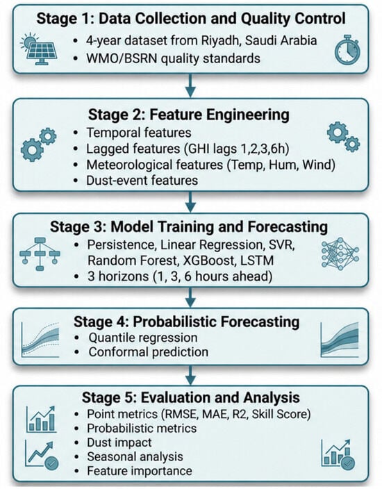
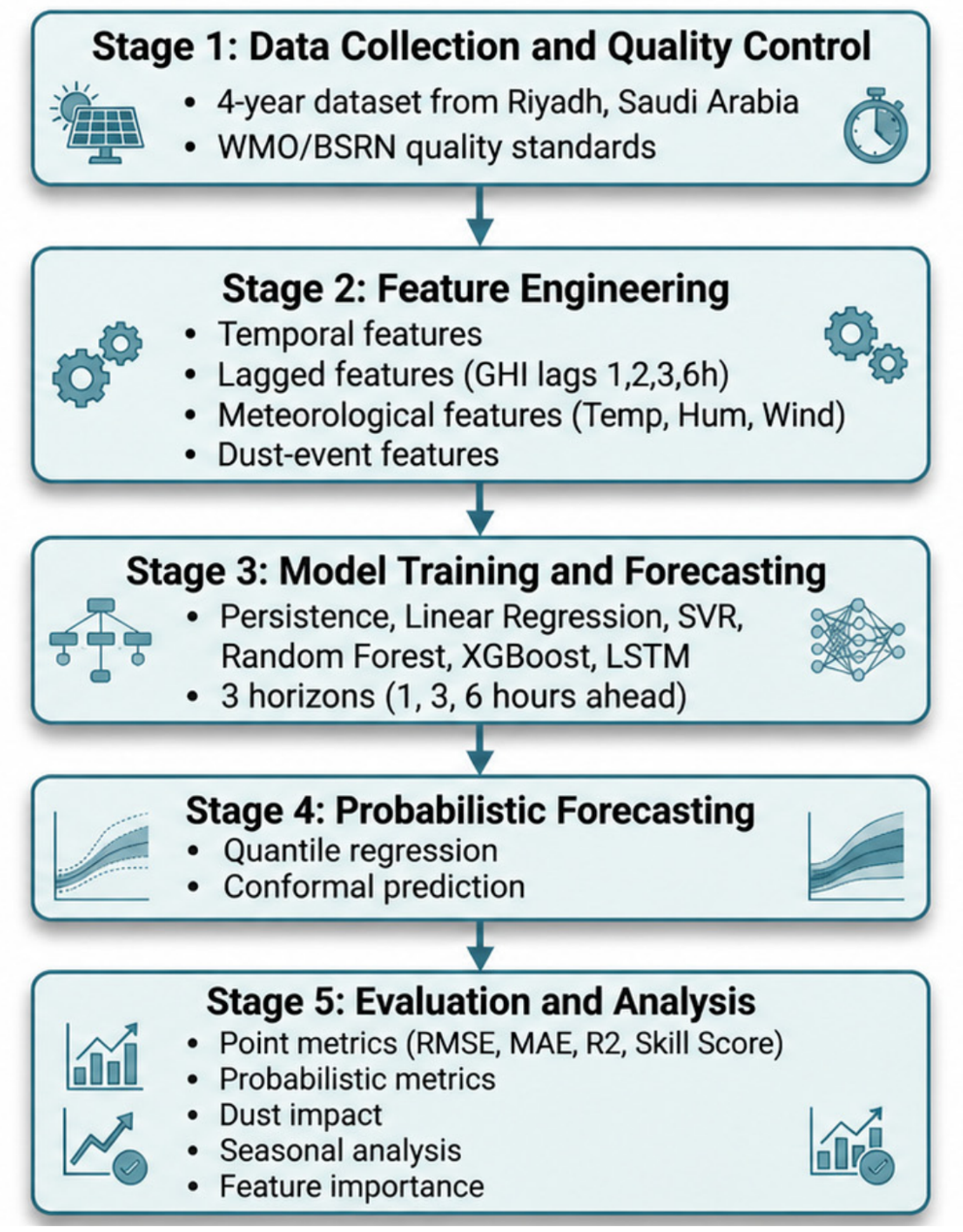
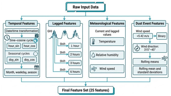
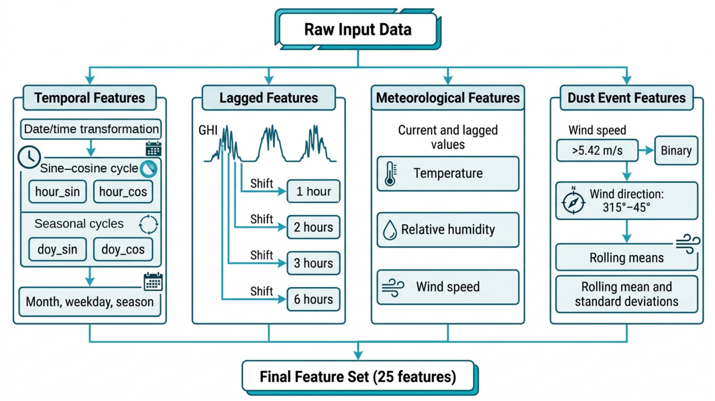
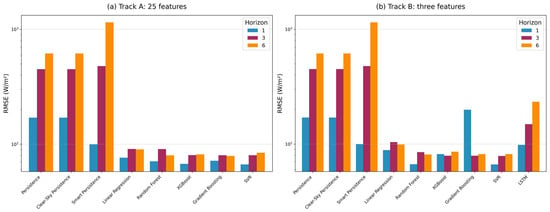
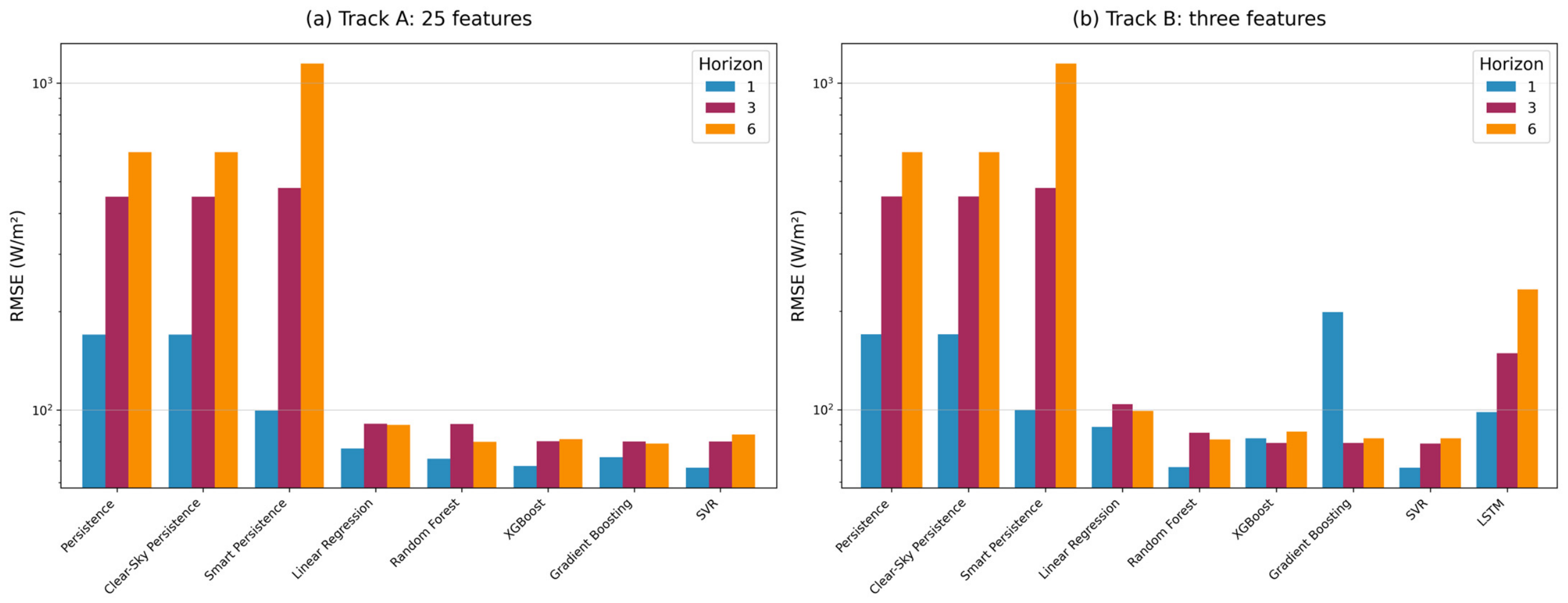
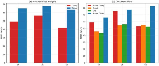
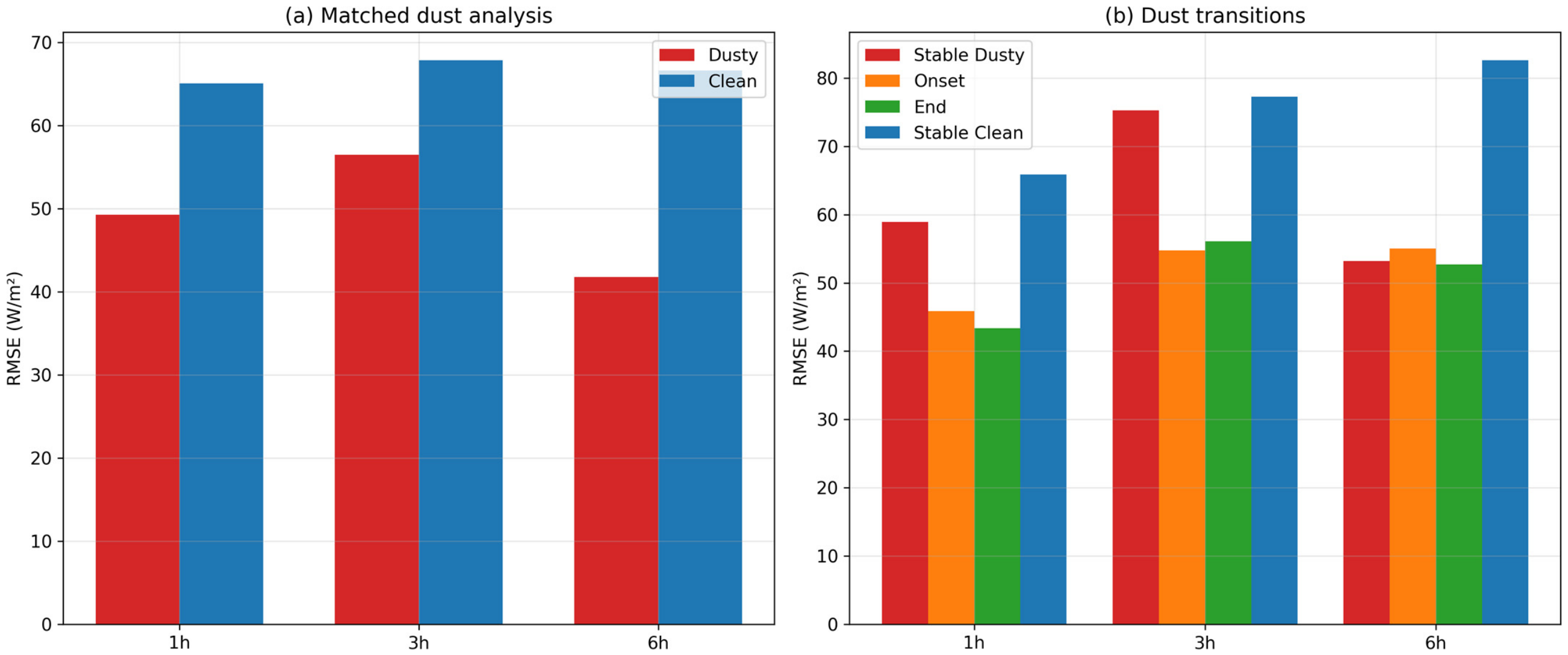
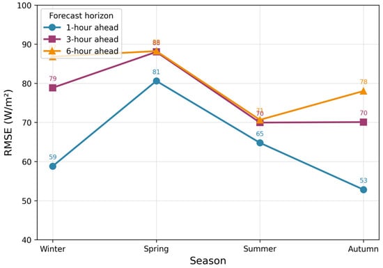
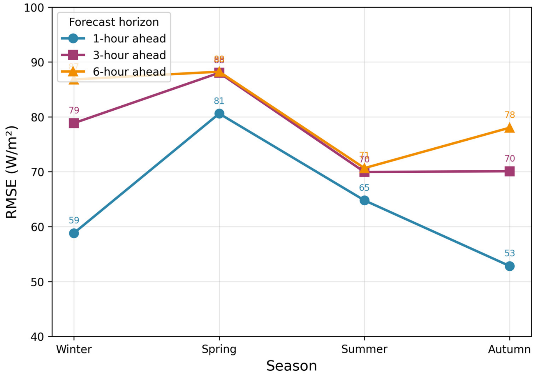
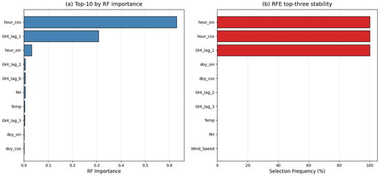
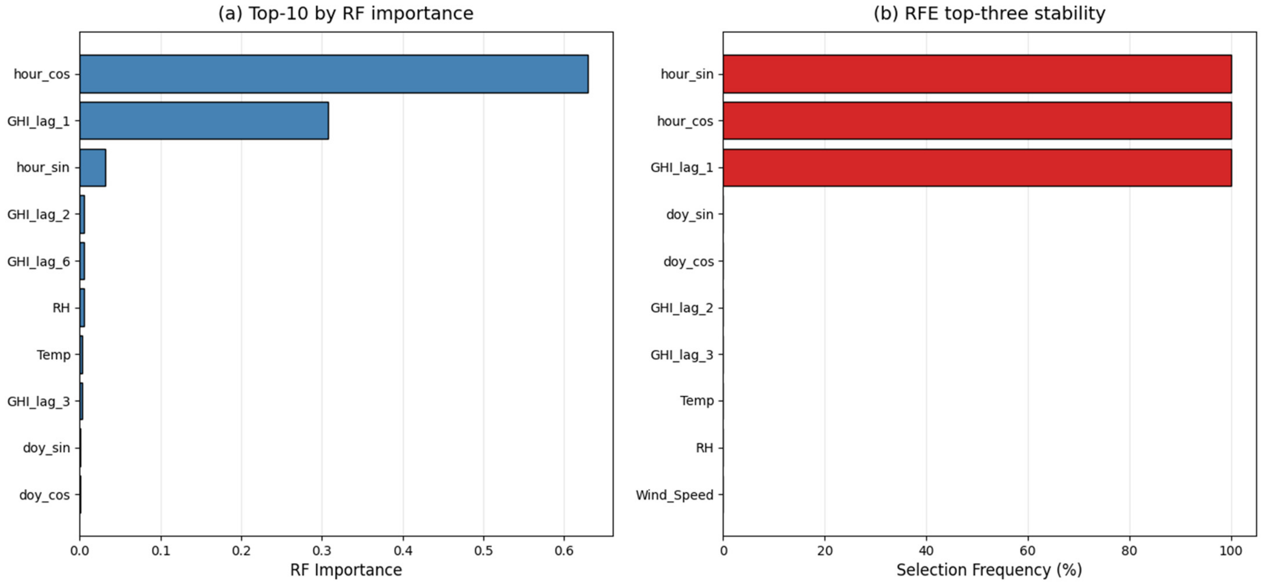
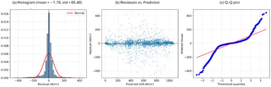
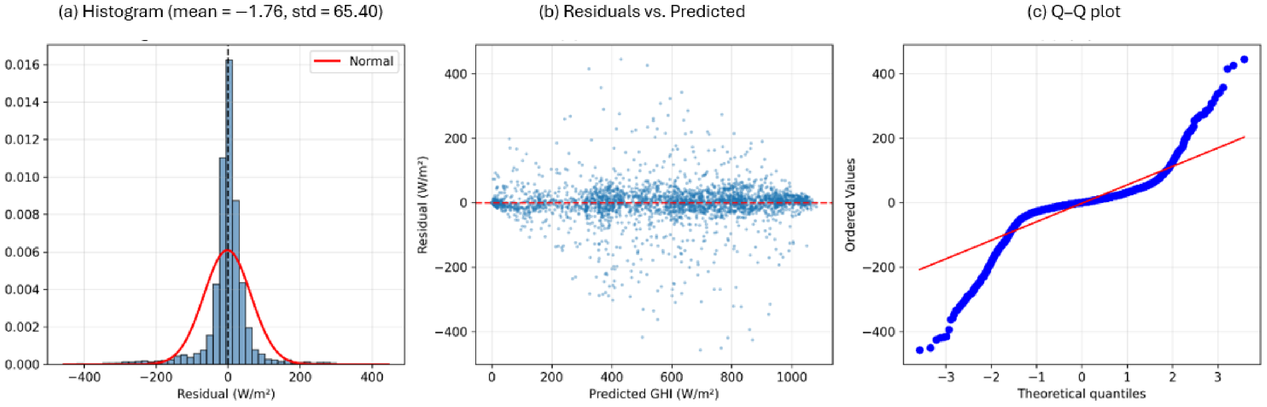
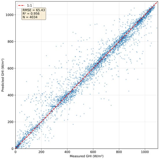
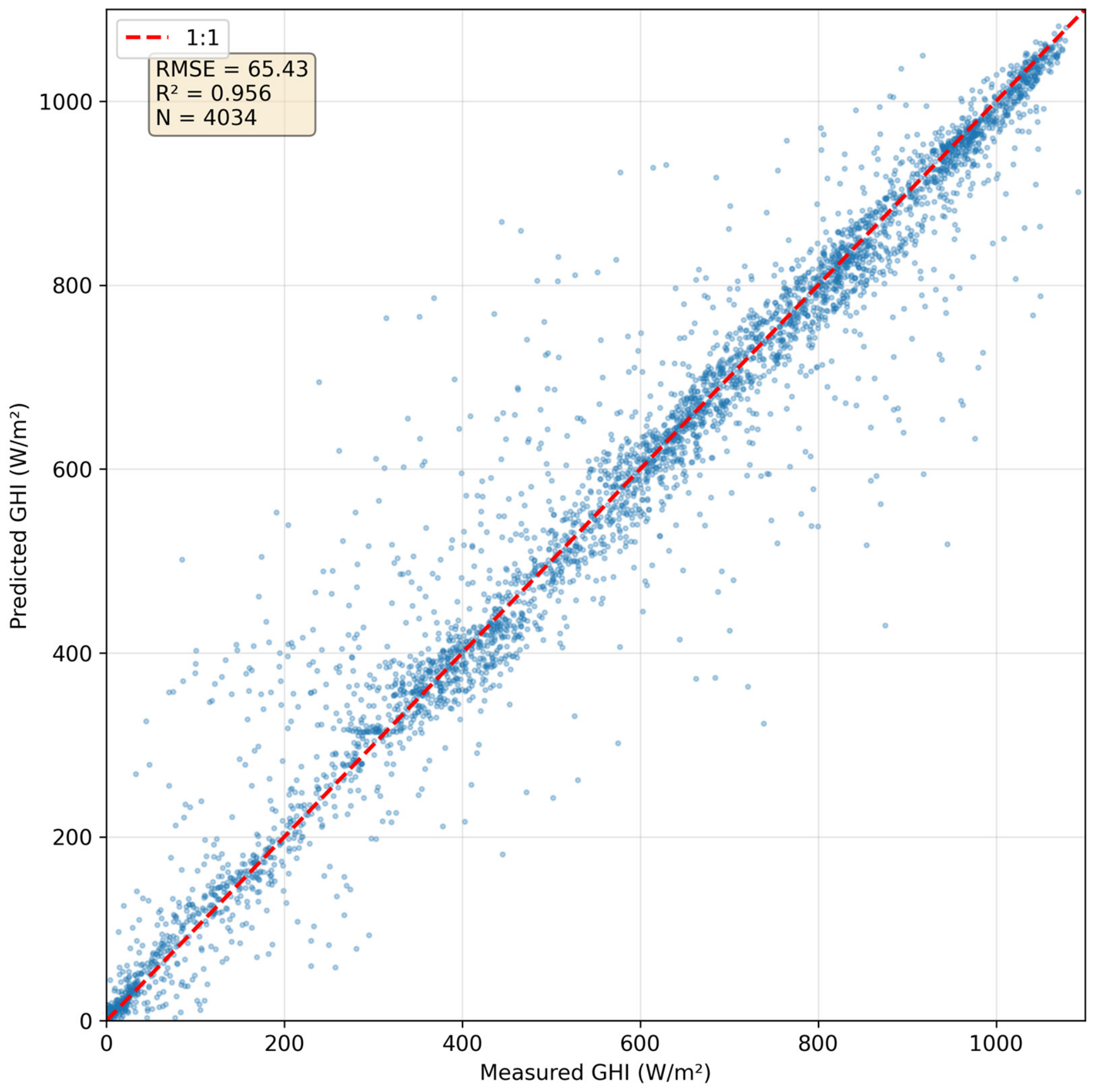
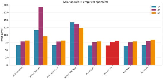
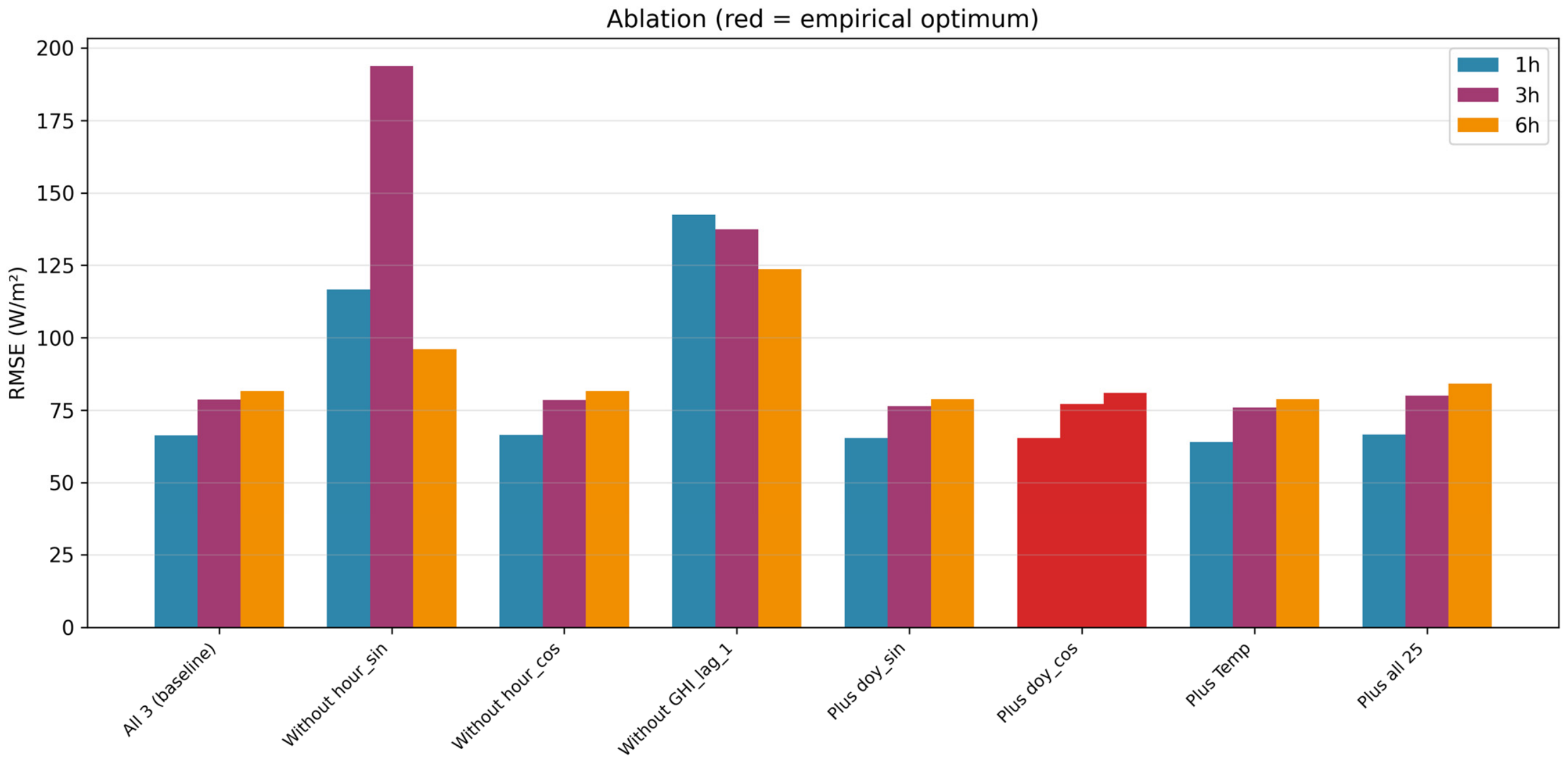
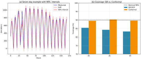
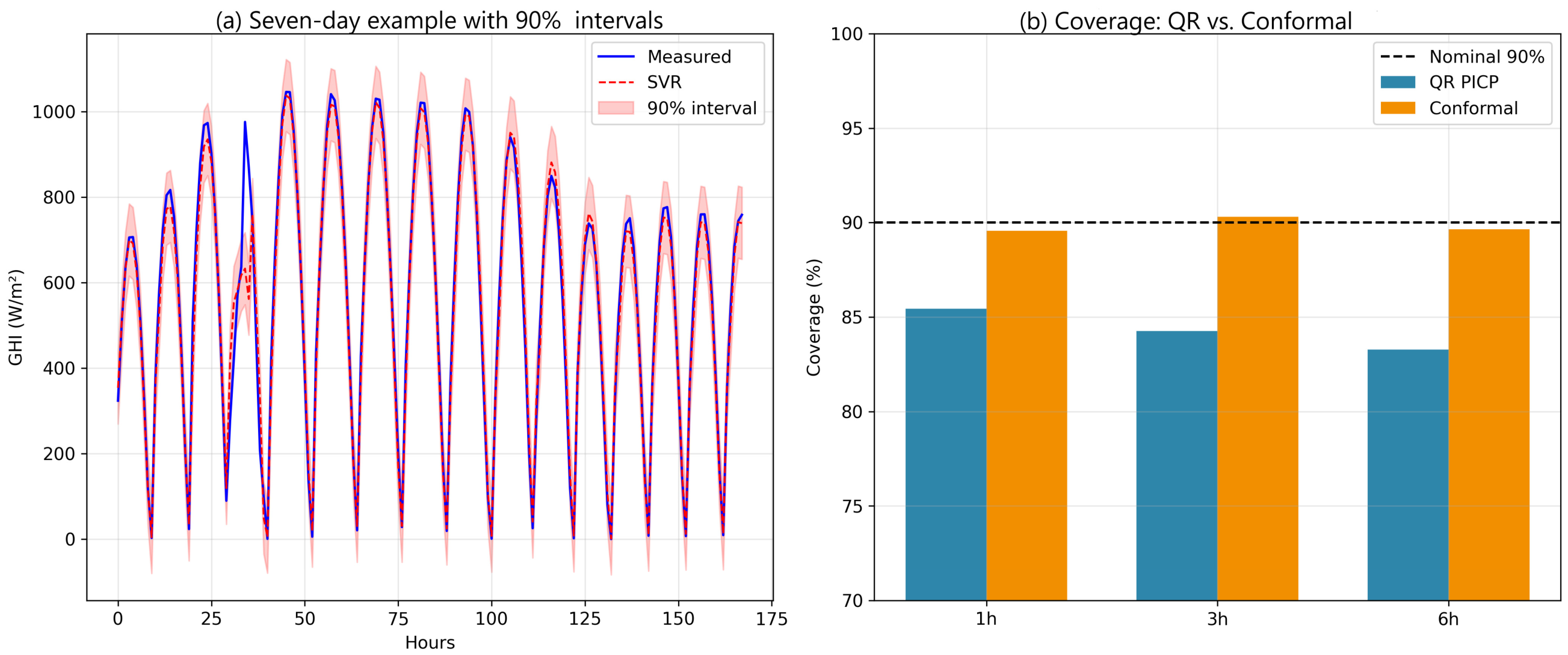
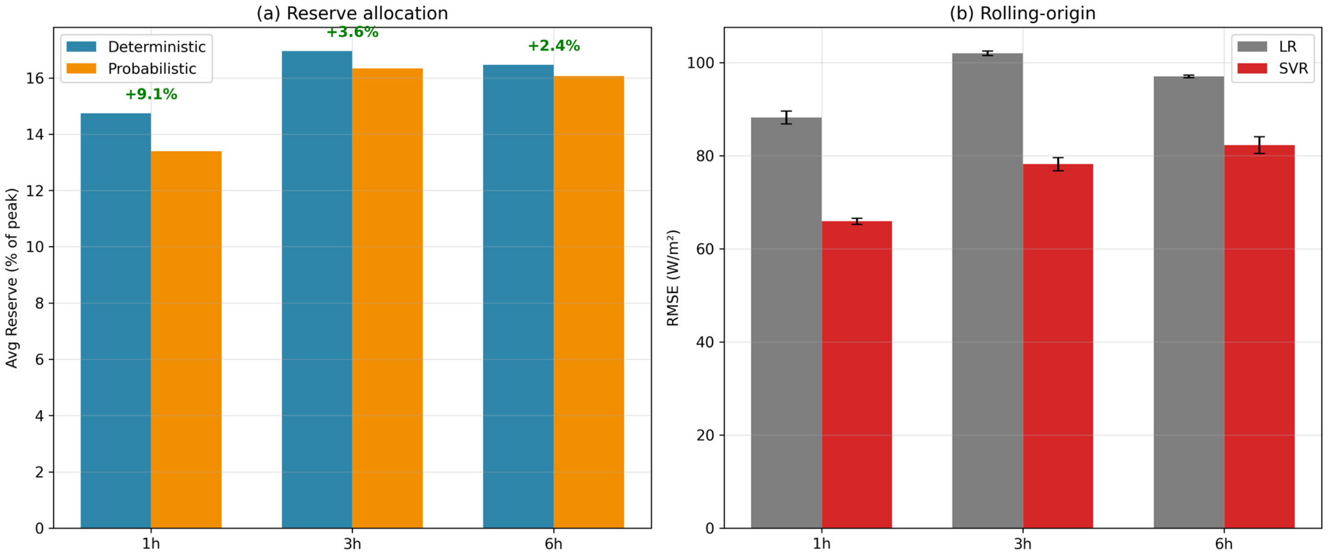

Disclaimer/Publisher’s Note: The statements, opinions and data contained in all publications are solely those of the individual author(s) and contributor(s) and not of MDPI and/or the editor(s). MDPI and/or the editor(s) disclaim responsibility for any injury to people or property resulting from any ideas, methods, instructions or products referred to in the content. |
© 2026 by the author. Licensee MDPI, Basel, Switzerland. This article is an open access article distributed under the terms and conditions of the Creative Commons Attribution (CC BY) license.