


Abstract
Wind energy has proven to be an effective component in decarbonizing electricity generation all over the world. As nations expand wind energy generation, they have been able to advance the goals of the Paris Climate Change Agreement, reducing greenhouse gas emissions. Wind energy provides significant sustainability benefits, helping to reduce pollutant emissions, improve the lives of local communities, and mitigate climate change. Additionally, it has become the lowest-cost energy source in many regions, even lower than natural gas, making it financially sustainable, not requiring economic subsidies. However, as wind energy expands, it becomes increasingly difficult to identify favorable locations for these facilities, since initial wind farms have occupied the most propitious sites and infrastructure has become more saturated. As electricity requirements grow in these locations, additional demand is being supplied by fossil fuel generation, as incremental wind energy becomes progressively more challenging to develop in these mature markets. This causes the carbon footprint from electric generation to grow, becoming detrimental to sustainability goals. This research aims to initiate the development of a spatio-temporal frameworks that will aid wind energy in mature markets to continue growing to support resilient renewable energy expansion. The proposal for frameworks applies geospatial data analytics to assess the potential growth of wind energy in mature markets, which may have reached levels of saturation. This will aid these mature markets to continue growing wind energy beyond current levels, to expand environmental and socio-economic benefits. Texas was studied in this analysis, applying the proposed method, to identify key factors that may improve sustainable operational results from wind energy. Results were promising, with the proposed framework identifying locations that may provide improved results to satisfy electricity demand in local markets. The study was able to identify locations and operational parameters that will aid stakeholders in future wind energy sustainable development decisions and promote resilient renewable energy growth in mature markets. Results from this study indicate the potential to expand wind energy development in Texas. For instance, the Coastal and South ERCOT Wind Regions reported a positive correlation coefficient between wind generation and electricity consumption, higher than 0.7. This study presents a case study-based framework that requires adaptation and external validation to be applied in other locations. The goal of the proposed spatio-temporal framework is to provide benefits to local communities, reducing greenhouse gas emissions, air pollution and water usage, and reducing the risk associated with climate change.
1. Introduction
Renewable energy provides a wide variety of critical benefits for the global economy and long-term sustainability. Compared with fossil fuels, it has a much smaller carbon footprint, reducing ecological degradation, pollution, and greenhouse gas emissions [1,2]. This greatly enhances living standards worldwide, fostering healthier communities, improving quality of life, and mitigating the impacts of climate change [3,4]. Wind and solar are two mature renewable energy technologies that have been deployed commercially worldwide. The continued expansion of these technologies has created a virtuous cycle that, over the last two decades, has led to significant improvements in equipment energy generation capacity, a decrease in potential environmental impacts, and significant energy cost reductions [5]. For these reasons, the growth of wind and solar energy has accelerated significantly, expanding to locations worldwide. They have become, in most cases, the lowest energy generation source, less expensive even than natural gas [6]. The Energy Information Administration reports that, for 2025, the Levelized Cost of Electricity (LCOE) for onshore wind in the US is $29.58, while combined-cycle natural gas has a LCOE of $64.55 [7]. As the cost and availability of fossil fuels are impacted by socio-political events, renewable energy, particularly wind and solar, has become a very attractive alternative. Nations that have significantly deployed wind and solar energy have been less affected by uncertainty stemming from supply restrictions on fossil fuels [8,9]. Therefore, it is expected that wind and solar energy will continue to grow in the near future.
These factors have accelerated the expansion of wind energy worldwide. However, there are regions that have developed utility-scale wind for many years, and as they seek to expand further, they may face challenges [10,11]. Older equipment, some of it installed more than 15 years ago, may be occupying some of the best wind locations, and it would be important to reassess how to grow this sector. One option, explored in prior research and implemented by developers, is repowering wind farms [12,13,14]. This requires replacing older, often smaller, equipment with modern and larger wind turbines. Wind farms with larger wind turbines require redrawing their layouts to account for greater turbine spacing and minimize wake effects. This may increase the cost and complexity of the new project, in many cases delay its implementation, or even make it unfeasible [13]. Furthermore, for many installed wind farms, their current peak generation times do not coincide with the higher demand among their consumers, reducing their usefulness and profitability [15,16]. Recent research indicates that some areas previously considered suboptimal for wind energy may now offer benefits when newer technologies are deployed, enabling wind farms to generate more energy during periods of higher consumption [17,18]. Furthermore, novel wind turbines, which are taller and have wider rotors, may be able to thrive in locations that previously were considered suboptimal for smaller equipment. As they can capture wind at higher altitudes, where wind speeds are normally higher, they may generate more energy and become more profitable [19,20].
Texas is the state in the United States with the highest installed wind capacity, accounting for 28% of the U.S. total wind electricity generation in 2024 [21]. Wind energy contributed significantly to the state’s electricity in 2023, being only second to natural gas [22]. With more than 230 wind farms comprising almost 20,000 wind turbines, Texas produces more electricity from wind than the next three states combined. There are several favorable reasons that have contributed to this extraordinary growth of wind energy in Texas over the last two decades. Excellent wind speeds, coupled with significant available land, have enabled the development of some of the largest wind farms in the US, such as Los Vientos, Roscoe, and Javelina Energy [23,24]. A critical component was the $7 billion Competitive Renewable Energy Zone (CREZ) infrastructure completed in 2014. This massive 3500-mile high-voltage transmission line infrastructure connects the wind-abundant Texas regions of the West and Panhandle with urban areas such as Dallas, Austin, and San Antonio, significantly incentivizing wind energy development [25,26]. These factors, combined with economic benefits to rural communities [27], the Texas deregulated energy market, advances in wind energy technology, and cost competitiveness with fossil fuels, have contributed to the massive growth of this industry [11].
However, as wind energy continues to grow in Texas, challenges are being experienced. Given that wind generation is dependent on meteorological conditions, farms in a region generate energy at similar times, creating congestion on transmission lines. With very little storage capacity, the only alternative is to curtail energy generation to avoid transmission overload, generating unused valuable capacity [28,29]. To continue growing in CREZ-dependent regions, additional investment in transmission lines or storage capacity would be needed, which would require substantial economic resources. Furthermore, because wind energy generated in the West and Panhandle regions peaks late at night, fossil fuels are needed to meet demand during high-consumption periods [30,31]. Therefore, generation in locations closer to urban areas in Texas, which may have more favorable generation timing and occur during high-consumption periods, becomes attractive [32,33]. Wind energy generated in offshore locations may be a better fit for Texas, considering the proximity of urban areas to the coast and the diurnal and stronger wind energy generation [34,35]. However, offshore wind projects are still in planning stages in Texas, and it is uncertain when they will be deployed. Therefore, placing wind turbines onshore near the coast may be a good alternative, as they could benefit from certain offshore wind characteristics and reduce installation and operational costs, which are typically higher for offshore wind [36,37].
The relevance of accelerating wind energy growth is underscored by the fact that it is the electricity generation method with the lowest carbon footprint, even lower than that of photovoltaic power. Gao et al. indicate that the wind manufacturing phase is the largest contributor of environmental impacts, accounting for 80% of the main pollutants and more than 78% of the total life-cycle footprint [38]. This study indicates that among the four compared energy production methods in the study, wind, solar, biomass, and thermal, wind has the lowest energy repayment time, 0.53 years, accounting for only 2.65% of the entire life cycle [38]. Therefore, accelerating the expansion of wind energy will enable nations to achieve the goals of the Paris Climate Change Agreement, significantly reducing greenhouse gas emissions and mitigating climate change [39]. Nations that have developed wind energy achieve significant environmental benefits, including healthier communities and reduced air emissions and pollution [40,41]. Optimizing wind farm placement and location significantly advances carbon footprint reduction [39,42]. More favorable wind farm locations increase the facility’s CF (Capacity Factor), generating additional electricity with the same equipment and advancing carbon footprint reduction. Furthermore, aligning generation times with periods of higher consumption reduces fossil-fuel electricity generation and decreases the overall carbon footprint [5,13,43]. Given that wind energy expansion has led to various constraints that have slowed progress toward sustainability goals, opening new areas to wind development is important for promoting sustainable development [44,45]. As new areas are required to continue growing wind energy, it would be important to provide stakeholders with a framework that allows them to select adequate locations that can be switched to sustainable energy-oriented development [44].
This study proposes developing a spatio-temporal framework to assess and promote wind energy in mature markets using geospatial data analytics. This case study-based framework could provide stakeholders with preliminary decision support to aid in the continuous growth of wind energy. As some regions have significantly grown wind energy, the initial favorable locations have been occupied with wind farms. Expanding into these markets becomes more challenging, as new potential locations must be carefully evaluated in light of local market requirements. This framework proposes identifying locally relevant spatio-temporal factors and selecting new locations based on these criteria. The use of geospatial data analytics enables stakeholders to conduct relevant assessments to select new locations that could achieve greater market success. The hypothesis of this study is that applying geospatial data analysis provides stakeholders with relevant insights for identifying new potential locations in mature wind markets. Therefore, the corresponding research question is: How can geospatial data analytics be applied to develop preliminary decision-support parameters to help stakeholders in energy-mature markets? To evaluate and further develop this framework, a case study for the United States was selected, with Texas identified as a mature wind energy market.
2. Materials and Methods
The proposed spatio-temporal framework integrates publicly available data from diverse US federal agencies and research institutions. This data is overlaid in a Geographic Information System (GIS) and developed into relational spatio-temporal systems to provide relevant analysis in the framework indicated in Figure 1. The framework is integrated into four functional bands, each forming a column in the flowchart. Each functional band (column) comprises diverse phases or activities required to complete the main functional band.
Figure 1.
Flow chart describing the different functional bands and phases or activities of the proposed spatio-temporal framework to assess wind energy development in mature markets. Assessment aims to identify locations that may be considered mature wind markets. Generation aims to assess the generation performance of the identified mature region. Demand aims to compare various factors related to wind generation. Expansion aims to evaluate potential strategies to additionally grow wind energy.
Many of these factors, such as CF, electricity demand, electricity pricing, and meteorological parameters, exhibit high variability over the course of the day and the year. For instance, in some locations, wind CF peaks at night, but electricity demand may be low then. Electricity demand may peak in the summer months, but wind generation may be low then. Therefore, including spatio-temporal analysis in the proposed framework provides stakeholders with additional elements to select locations for wind energy development.
Assessment is the first functional band of the proposed spatio-temporal framework, comprising three phases or activities: identify, select, and grow. The objective of this first functional band is to identify regions that have reached incremental wind energy saturation, thereby becoming mature wind markets. Mature wind energy markets can therefore be defined as geographical locations that, for a variety of reasons, are experiencing difficulties in further growing wind energy. An area that has experienced significant reductions in annual new wind capacity or turbine additions for more than one year due to limiting factors may be considered a mature wind market. Analysis in the results section will describe a significant reduction in the installation of new wind turbines and in wind capacity in Texas since 2023. There are a wide variety of factors that may limit wind energy growth in a particular location. Examples of these limiting factors include saturation of required infrastructure, technology feasibility challenges, or misalignment between generation and consumption. In many mature markets, locations historically considered favorable are already occupied by older, less efficient wind farms. Diverse worldwide locations may have distinct limiting factors; therefore, one of the initial tasks of the proposed spatio-temporal framework is to identify these locations and their limiting factors. The proposed framework provides stakeholders with additional tools to assess continued growth in wind energy.
Publicly available information on installed capacity, wind electricity generation, and the resource’s historical growth is analyzed and compared with other locations to identify mature markets. In the case of the US, the United States Wind Turbine Database (USWTDB) provided by the US Geological Survey (USGS) [46] and data on wind electricity generation provided by the Energy Information Administration [47] were integrated into the proposed Geospatial Data Analytics system.
Once the maturity status of a location has been determined, the second functional band in the proposed spatio-temporal framework evaluates wind farm generation performance. This is, in turn, integrated by three phases or activities: Placement, Distance, and Performance. This functional band aims to assess the generation performance of the identified mature region and evaluate potential strategies to expand wind energy, as well as the critical factors impacting this growth. Considering that power output from wind farms depends on their geographic placement due to diverse local meteorological factors. Texas wind performance can be evaluated using data provided by the Electric Reliability Council of Texas (ERCOT). ERCOT is an independent system operator (ISO) in the US that controls the electrical grid in Texas, managing 90% of the state’s electric demand. For wind energy management, ERCOT has created five wind regions. Each of these regions has similar wind generation conditions, creating relative uniformity in the performance of wind farms within their boundaries. This allows ERCOT to optimize the management of wind resources through diverse time periods and seasons [48].
Wind electricity demand analysis is the third functional band of the proposed spatio-temporal framework, comprising three activities or phases: time-based analysis, location-based analysis, and contrasting wind generation with consumption. The goal of this functional band is to compare various factors related to wind generation with variable electricity demand to evaluate which factors could better meet the demand. The challenges arise from potential divergences in the generation and consumption times of wind electricity. Since energy storage capacity is very limited and hourly electricity consumption is not uniform throughout the day, matching generation to consumption improves the benefits of wind energy. Electricity demand in the US increases in the afternoons, as most households return from work, and decreases at night [49]. This is important, as wind energy is highly variable and depends on wind patterns. This creates one of the biggest challenges for wind energy: the divergence between electricity generation and consumption. For these reasons, exploring hourly wind generation is relevant, as it helps identify factors such as locations, time periods, or technology where wind energy aligns better with consumption, thereby improving societal benefits for the sector [50].
The last functional band of the proposed spatio-temporal framework is Expansion, which aims to evaluate potential strategies to additionally grow wind energy in the mature location. It is integrated into three phases or activities: pairing, profile, and resolution. In this functional band, the factors selected by the framework are paired to identify which of them could enable a wind farm to improve benefits for all stakeholders. In this case, hourly electricity demand and generation are segmented by locations and seasons to evaluate their alignment. This analysis will aid stakeholders in selecting locations that may improve wind farm operations and development. Publicly available data from ERCOT, USWTDB, the US Energy Information Administration, and the National Renewable Energy Laboratory (NREL) were integrated and overlaid within the proposed framework to generate these analyses [46,47,48,51].
As previously indicated, each geographic location may have distinct limiting factors that constrain wind energy growth. For each individual location, the two initial functional bands of the proposed framework, Assessment and Generation, will allow stakeholders to identify individual limiting factors. With this information, the required databases and information will be identified, collected, and integrated into the system. However, it is important to note that this study presents a case-study-based framework that requires adaptation and external validation for potential application in other locations.
3. Results
The initial functional band in the proposed spatio-temporal framework to promote wind energy in mature markets is to assess a broader geographic area to identify potential locations that have reached this stage. For the United States (US), assessing the performance of each State is a useful approach to comparing and identifying locations that have reached maturity in wind energy development. It is worth noting that wind energy development in the US has been uneven over the last four decades. Initially, there was a very significant impetus to implement wind energy in response to the oil crisis in the 1970s. California installed the first commercial wind farms, composed of hundreds of small wind turbines, at Altamont Pass, Tehachapi Pass, and San Gorgonio Pass. However, at the start of the XXI century, more modern and larger equipment was installed in other states, including Texas, Iowa, Oklahoma, and Kansas. To identify states with higher wind energy penetration, data from the USWTDB [46] were integrated into the GIS to evaluate both wind turbines and CF at each location. Figure 2 shows the current installed wind turbines across different states, including the number of turbines and the total state capacity (GW). Texas has the most wind turbines, accounting for more than 26% of the nation’s turbines and almost 28% of all installed wind capacity. The number of wind turbines and installed capacity provide an initial basis for identifying regions with the highest market penetration of this renewable resource. This allows for additional contrast analysis by maturity level for each location.
Figure 2.
Wind energy installed in states in the continental US: (a) number of wind turbines; (b) installed capacity (GW).
Comparison with other geographical locations is relevant for the selection segment of the assessment functional band. This is accomplished by contrasting the level of wind development against the broader geography. Data on wind electricity generation, provided by the Energy Information Administration [47], were integrated into the GIS and used to develop Figure 3. This contrasting analysis provides insight into the market penetration of wind energy for each state. Results indicate that Texas generates 28% of all US electricity from wind, nearly equal to the combined output of the next four top-generating states. This significant difference between Texas and other states in wind energy generation is the product of more than two decades of incremental development in this sector in Texas. This has been fostered by a combination of extensive public infrastructure investment, a supportive regulatory environment, and favorable environmental and physical conditions. With these elements, it is possible to select Texas as the most mature wind market in the US.
Figure 3.
Wind electricity generation in 2025 for US states. (a) Map of electricity generated from wind. (b) Pie chart of states representing more than two-thirds of wind electricity generation.
The potential for wind energy growth in Texas is explored in the third band, Growth Potential, of the first functional band (assessment) of the proposed spatio-temporal framework. To evaluate the historical evolution of wind electricity generation and its market penetration, EIA electricity generation data [47] were used. Figure 4a highlights the high growth pace of electricity generated from wind in Texas since 2005, at a much faster pace than all the other US states. Texas has been growing by almost 7 TWh per year on average over the last two decades, while the other top-producing states have grown by less than 2 TWh per year. On the other hand, results from Figure 4b show that since 2021, Iowa and South Dakota have met more than half of their electricity demand from wind, with this share recently exceeding 60%. Furthermore, Kansas has exceeded the 50% threshold in recent years, while Oklahoma has broken the 40% barrier. Conversely, Texas, with 28% of the nation’s wind electricity generation, meets only 22% of its electricity demand with wind, indicating lower market penetration than in other states. This highlights the available opportunities in Texas to continue expanding wind energy to satisfy its energy demands. Texas wind energy installed capacity may be the largest in the nation, but from the demand perspective, the framework indicates significant growth potential.
Figure 4.
Wind electricity generation growth from 2001–2025 for top eight generating states in US states: (a) line chart of annual growth; (b) bar chart of annual growth with bars in each state corresponding to consecutive years from 2001–2025, each year having been assigned a corresponding color.
As previously indicated in the Methods Section, once a location’s maturity status has been determined, the second functional band of the proposed framework evaluates wind farm generation performance. Texas wind performance can be evaluated using ERCOT data, which has created five wind regions (Figure 5) to manage wind energy generation. Similar wind generation conditions are present across each ERCOT wind region, enabling improved management of Texas wind resources. On the other hand, as previously mentioned in the Methods Section, to manage electricity demand, ERCOT uses a different division of the state, with eight ERCOT Weather Zones, which can create a potential disconnect between electricity demand and wind generation. In Texas, the greatest demand for electricity occurs in the Texas Triangle, formed by Houston, Dallas, Austin, and San Antonio, which together comprise more than 20 million people (two-thirds of the state’s population). Figure 5 presents the number of wind turbines and the installed capacity in each wind region, combining data from the USWTDB [46] and the ERCOT wind regions [48]. The map in Figure 5a shows that, for 2025, of the almost 19,500 wind turbines in Texas, close to 75% are installed in the West and Panhandle wind regions. Figure 5b indicates that, of the almost 44 GW of wind capacity in Texas, more than 76% is in the West and Panhandle wind regions. Therefore, it is important to assess the potential to expand wind development in regions near these urban areas, which may have a better synchronicity with energy demand and require shorter transmission infrastructure.
Figure 5.
ERCOT Wind Regions in Texas with the largest urban areas: (a) number of wind turbines per wind region; (b) installed capacity per region (GW).
Figure 6 shows the development of wind energy in Texas over time, providing clear insight into the reasons for the high concentration of wind energy in the West and Panhandle regions. These results further reinforce Texas’s status as a mature wind energy market, with significant declines in new wind turbine installations and wind capacity since 2023. Results presented in these figures show that, in its initial years, turbines were installed in large numbers in the West and Panhandle wind regions, owing to favorable wind speeds and the widespread availability of land for developing large wind farms. It was not until 2009 that 237 wind turbines were installed in the Coastal wind region, representing 18% of all wind turbines installed in Texas that year. The next year, 48% of all turbines installed in Texas were located in the Coastal wind region, and in 2012, 289 were installed there, representing 32% of the state’s wind turbines that year. This showcases the initial focus on the West and Panhandle areas, which gradually shifted to include other areas, particularly the Coastal and South wind regions. Figure 6b shows that although there has been a reduction in the number of new wind turbines since 2023, the participation from the Coastal and South wind region has been significant. In 2025, the highest proportion of turbines (39%) was installed in the Coastal wind region, which, combined with the 29% in the neighboring South area, eclipses the 18% located in the West area that year. Interest in the Coastal and South wind regions may be related to reports indicating that electricity transmission lines have experienced congestion during periods of high wind energy production and low demand [23,52]. Therefore, transmission line assessments are a relevant factor in evaluating potential avenues for growing wind energy in Texas.
Figure 6.
ERCOT wind regions in Texas. (a) Number of wind turbines per year and wind region. (b) Proportion of installed wind turbines per year and wind region. Red line in both charts corresponds to cumulative growth.
Evaluating installed wind capacity per wind region in Texas over time provides additional insight for the location analysis of the proposed spatio-temporal framework. It enables the system to identify factors that may affect the future development of wind energy. Figure 7 shows the installed Name Plate Capacity. The reduction in the installed number of turbines from 2022 to 2025 is 75%, but in NPC terms, it is only 72%. Furthermore, the results presented in Figure 7b reinforce previous insights into the potential to expand other wind regions in Texas, particularly the Coastal and South wind regions. In 2025, installed capacity in the Coastal and South areas accounted for 78% (45% and 33%, respectively), which is much higher than the combined 68% for the Coastal and South wind regions when accounting for individual wind turbines. This indicates that these two wind regions are installing larger NPC wind turbines to improve wind energy extraction. Evaluating these results indicates potential to grow this industry in other wind regions beyond the West and Panhandle areas.
Figure 7.
ERCOT wind regions in Texas. (a) Installed wind capacity per year and wind region. (b) Proportion of installed wind capacity per year and wind region. Red line in both charts corresponds to cumulative growth.
The distance analysis is the second activity of the generation functional band of the proposed framework. As indicated, wind energy is highly dependent on local meteorological conditions; therefore, turbines may be located far from consumption centers. In Texas, delivering electricity from wind farms to large urban areas is one of the main challenges for its development. For several decades, significant public investment has been allocated to this task, resulting in a very robust high-transmission-line network of almost 22,000 km, as shown in Figure 8. The map shown in Figure 8a depicts high transmission lines (345-kV) installed in the ERCOT wind region. Data from the Electric Power Transmission Lines [53] were evaluated to develop classifications of high-power transmission lines by the wind regions they serve. To ascertain the ERCOT wind region to which transmission lines correspond, a join attribute by location and clip operations were performed on the line shapefile containing the transmission lines. Results from this analysis are presented in Figure 8b, showing that 54% of these transmission lines connect to wind power from the West and Panhandle wind regions, compared with only 17% from the Coastal and South wind regions. This is relevant because transmission lines serving the West and Panhandle have been reported to be highly congested due to the significant growth of wind farms in these regions. This has led to requests to curtail wind farms in these regions and to a significant increase in demand for natural gas electricity to meet the growing demand generated by economic growth in the state [54]. To further expand wind energy in these areas, additional investments in high-power transmission lines would be required. This would require a massive infusion of financial resources, considering the long distances involved in the process. Therefore, it may be advantageous to consider wind energy for additional growth in regions closer to urban centers in Texas, such as the Coastal and South wind regions, which align with findings from previous analyses of the proposed framework.
Figure 8.
High-voltage transmission lines (345-kV) in Texas, classified according to the wind regions being connected. (a) Texas map with the ERCOT wind regions. (b) Pie chart indicating transmission lines corresponding to each classification.
The Electric Reliability Council of Texas (ERCOT) provides hourly power profiles of operational and planned wind energy farms in Texas from 1980 to 2023 [55,56]. This information was integrated into the GIS to ascertain the ERCOT wind region for the facilities and create a comprehensive profile evaluating the CF of each wind farm and the distance to each of the four major cities comprising the Texas Triangle. Figure 9 shows a box plot and whiskers that present results for this analysis, with the ERCOT wind region shown in different colors as described in the chart legend and the diverse CF ranges shown on the x-axis. Results from this analysis indicate that the Coastal wind region is convenient for Houston, San Antonio, and Austin, with many wind farms with a CF (above 45%) at greater distances. Additionally, the South wind region is a good option for Houston, San Antonio, and Austin, with some higher-capacity wind farms for Houston indicating longer distances. On the other hand, the West wind region is a better option for Dallas regarding wind farms with a higher CF. The North wind region, which is a good option for all of the cities, especially Dallas, has not been extensively developed for wind energy generation. Based on the results of this distance evaluation, further analysis will be performed as part of the proposed framework to assess the potential to develop wind in alternative, favorable locations. This analysis will allow developers to select the location for wind farm investment that best fits the particular city being served.
Figure 9.
Box plot and whiskers on CF (Capacity Factor) for wind farms according to ERCOT wind regions and distance from Texas major cities: (a) Austin; (b) Dallas; (c) Houston; (d) San Antonio.
Electricity demand analysis is the third functional band in the proposed spatio-temporal framework for evaluating the potential for wind energy growth in Texas. For this analysis, the first element involves time-based evaluation of demand. Considering that hourly electricity consumption has high hourly variability during the day, increasing in the afternoons and decreasing during the workday and night hours. As previously indicated, this creates one of the biggest challenges for wind energy: divergence between electricity generation and consumption. This analysis evaluates hourly wind generation and electricity consumption to identify locations where the two are strongly aligned. Figure 10a shows the eight ERCOT weather zones with the large urban areas of the Texas Triangle, which, as previously indicated, are significantly different from the ERCOT wind regions. This highlights the divergence between wind generation and electricity consumption. To evaluate which wind regions may be a better fit for consumption patterns, an hourly electricity consumption analysis was performed, as shown in Figure 10b. This figure presents the three quartiles (Q1—25%, Q2—50%, and Q3—75%) of hourly electricity demand reported by ERCOT, based on data from January 2002 to March 2026 [57]. The results indicate a consumption pattern similar to other locations in the US, with the afternoon hours between 14 and 20 having the highest demand, peaking at 16 and 17 h in Q2 and Q3. This analysis allows for comparison of wind energy generation across wind regions and identifies areas with a better temporal fit between wind generation and electricity consumption.
Figure 10.
ERCOT considers weather zones to characterize electricity demand. (a) Map of ERCOT weather zones. (b) Hourly electricity demand for ERCOT in quartiles, considering data from January 2002 to March 2026.
Electricity demand varies by location, leading to the second phase or activity of the third functional band of the proposed spatio-temporal framework. Identifying locations that may benefit from wind energy generation based on their location and consumption time patterns can help stakeholders make decisions to grow this industry. Considering that Coastal and South Central ERCOT Wind areas are a good fit in terms of distance for Houston, San Antonio, and, in some instances, Austin, demand analysis for these locations would be relevant to the proposed framework. Those cities are located in the South Central and Coast ERCOT weather zones to evaluate electricity consumption. The charts in Figure 11 show quartile results based on ERCOT data on electricity demand from January 2002 to March 2026 [55]. The pattern presented by these charts highlights the daily variability of electricity consumption in these locations. For the Coast weather zone (Houston), shown in Figure 11a, peak consumption times occur between 15 and 18 h with a 36–38% increase in consumption in Q2 compared with the lowest daily value. For Q3, variability increases in the Coast weather zone by 47–49% when comparing consumption over 15–18 h to the lowest daily consumption. Figure 11b shows the analysis for the South Central weather zone, which includes San Antonio and Austin. Results for Q2 and Q3 show the highest variability when comparing the highest consumption times with the lowest demand time. For Q2, the highest consumption occurs at 17–20 h, with increases of 47–50% compared with the lowest daily demand. For Q3, the increase is larger during the high-consumption period, between 16–19 h, where consumption increases by 58–61% relative to the lowest daily value. Since wind regions exhibit divergent power output depending on local weather conditions, it is important to evaluate whether wind regions near these urban areas can better meet these high-consumption periods.
Figure 11.
Electricity demand in quartiles considering data from January 2002 to March 2026 for two ERCOT weather zones: (a) Coast; (b) South Central.
The last section of the third functional band of the proposed framework involves contrasting wind generation with electricity consumption to better characterize the challenges presented. In this analysis, the goal is to identify the characteristics developers should consider when evaluating investments in wind facilities. To better understand the challenges in meeting electricity demand from wind energy, a comparison of hourly demand and wind CF, classified by month, is relevant, as shown in Figure 12. This analysis indicates that across the ERCOT wind region, the highest hourly electricity demand occurs during the summer months of June, July, and August. However, when comparing wind CF across the state, these months have among the lowest yearly values. Figure 12a indicates a clear difference in electricity demand across trimesters. The first trimester of the year shows low consumption; the second trimester shows a gradual monthly increase, peaking in the summer. Figure 12b shows CF characterized by trimesters, with the second trimester showing declining values that reach lower levels in the third trimester. Evaluating the fitness of wind energy in the Coastal wind region by trimester, compared with consumption during this period, will allow developers to set additional decision criteria. Therefore, expanding the analysis to assess whether some wind regions, particularly coastal areas, have higher CF during the hours of highest consumption in these months would be important.
Figure 12.
Comparison between monthly (a) electricity demand and (b) Wind Farms CF (Capacity Factor).
4. Discussion
Once relevant criteria have been identified in the first three functional bands of the proposed spatio-temporal framework, it is important to apply them to select favorable paths for wind energy expansion. These criteria and parameters are evaluated in the fourth functional band of the proposed framework to select expansion paths for this energy resource in mature markets. The first activity of this last path is to identify pairing criteria that can support more successful wind farm development. In this case, hourly electricity demand is paired with wind energy generation across the distinct ERCOT areas to align them so wind can improve output during high-consumption periods. For this analysis, hourly power profiles for operational and planned wind energy farms in Texas from 1980 to 2023 [55,56] were evaluated, and the relevant results are presented in Figure 13. Hourly CF was preliminarily evaluated to ascertain times of higher power output to meet the demand of nearby urban areas. The overall CF for the state of Texas reflects higher production in the middle of the night, 21–2 h. The median (Q2) for the highest production times is between 40.8% and 44.5%, while the third quartile ranges from 72.4% to 74.4%. For the critical high-consumption times between 15–19 h, the median CF for the state is only 25.7–34.5%, and the third quartile is 59.2–65%. These values are in the lower half of the hourly CF, reflecting low generation capacity during periods of higher consumption. However, when focusing only on wind energy production for the ERCOT Coastal wind region, the results are significantly different and very promising in regard to electricity demand. The highest CF for the year is between 15–18 h, with Q2 (median) at 41.7–47.5% and Q3 (third quartile) at 68.6–76.2%. This aligns well with the highest consumption times for the Coast and South Central weather zones, which include Houston, San Antonio, and Austin, as shown in the previous Figure 10. Considering the shorter distances to these wind farms from the mentioned urban centers, this may represent an opportunity to expand wind energy development.
Figure 13.
Wind Farms CF (Capacity Factor) calculated from ERCOT for hourly power profiles for (a) Texas state and (b) Coastal ERCOT wind region.
As a continuation of the current pairing activity, the framework emphasizes the importance of determining whether any other ERCOT wind region has performance similar to that of the Coastal Region, thereby providing a better fit for electricity consumption. To expand the analysis of the pairing process, Figure 14 was developed. The comparative assessment presented in Figure 14a for all median values (Q2) of wind farms in each wind region clearly demonstrates that the Coastal wind region behaves differently from the general behavior of other Texas onshore wind farms. As previously indicated, this is particularly important given the strong relationship between electricity demand in urban areas and their proximity to these consumption centers. Figure 14b shows the results for the third quartile (Q3) CF, reinforcing the adequacy of Coastal resources to meet electricity demand. It is important to note that, in addition to the Coastal wind region, other wind regions (South, North, and Panhandle) also have significant Q3 CF during the 15–18-h period, with values around 60%. Of these additional regions, the South may be the most relevant for further analysis, considering the long distance from the Panhandle wind region to many urban areas and the scarcity of areas with good wind resources in the North wind region. The South wind region, adjacent to the Coastal wind region, could offer additional wind development opportunities.
Figure 14.
Wind Farms CF (Capacity Factor) calculated from ERCOT for hourly power profiles for all ERCOT wind regions: (a) Median—Q2; (b) Third Quartile—Q3.
Figure 15 presents additional statistical analysis on the alignment between wind energy generation and electricity consumption in Texas. Figure 15a presents the hourly CF for wind farms in Texas as reported by the ERCOT operational and planned wind energy farms in Texas from 1980 to 2023 [55,56] as bar charts. The quartiles for hourly electricity demand reported by ERCOT are shown as line charts and are based on data from January 2002 to March 2026 [57]. From this chart, it is possible to observe that only the Coastal wind region and, to a smaller extent, the South wind region increase CF, and therefore generation, during the high demand period of 14–20 h. This chart shows that these two wind regions are more closely aligned with electricity demand. Figure 15b reports the correlation coefficient between average hourly CF and ERCOT electricity consumption across the corresponding quantiles (Q1: 25%, Q2: 50%, and Q3: 75%). The correlation coefficients confirm, in analytical form, the high alignment within the Coastal wind region. All coefficients are greater than 0.7 in this wind region, indicating a strong positive alignment between the two variables. This clearly indicates that wind generation increases and electricity demand increases, which is a very desirable behavior. All other wind regions, except the south wind region, have a negative correlation coefficient, indicating misaligned timing and a potential risk of curtailment and lower electricity prices. Therefore, this statistical analysis creates a relevant focus on the potential to develop the Coastal and South wind regions.
Figure 15.
ERCOT Wind Farms CF (Capacity Factor) compared with ERCOT electricity consumption. (a) Comparison chart. Electricity consumption (MWh) as lines and CF as bar charts. (b) The table reports the correlation coefficient between average hourly CF and electricity consumption (MWh).
The hourly electricity demand profiled by trimesters is shown in Figure 16. This analysis is part of the second activity of the last functional band of the proposed framework. It indicates that during the first and last trimesters of the year, Figure 16a,d, hourly electricity demand has lower variability when compared with the other two trimesters. On the other hand, the second and third trimesters, shown in Figure 16b,c, indicate significant variability, with large demand increases in the afternoons, when families return home after the workday. The 15–20 h. periods for both trimesters are peak consumption times, when electricity generation would need to be ramped up significantly. If no wind energy is available at these times, other electricity generation sources, in many cases, hydrocarbon-based, would need to be brought online. Therefore, if high levels of wind energy output could coincide with these time periods, significant benefits could be realized.
Figure 16.
Hourly ERCOT electricity demand by trimesters: (a) first trimester; (b) second trimester; (c) third trimester; (d) fourth trimester.
As part of the profile analysis regarding CF for the Coastal wind region, Figure 17 presents hourly wind farm results for comparison with electricity demand. These results showcase alignment with the hourly electricity demand presented in the previous analysis. The CF for the first and last trimesters of the year indicates lower variability when compared with the remaining trimesters, which is a similar pattern to that of electricity demand per trimester, shown in the preceding section. Furthermore, the second and third trimesters present a significant increase in CF for the afternoon hours, similar to the corresponding trimesters for electricity demand. This analysis provides relevant information to diverse stakeholders to identify locations that better align with energy consumption patterns and are closer in distance. Additionally, as electricity prices rise during peak consumption periods, these wind farms could earn higher revenue by supplying electricity during those periods. Using the geospatial data analytics platform to make these decisions will provide developers with the information needed to create successful wind farms that deliver greater benefits to local communities and renewable energy investors.
Figure 17.
Hourly wind CF (Capacity Factor) for the ERCOT Coastal wind region by trimesters: (a) first trimester; (b) second trimester; (c) third trimester; (d) fourth trimester.
Previous analyses have shown that electricity demands in Texas peak in the afternoons, between 14–20 h. Higher demand typically leads to higher electricity prices, which is an important incentive to generate wind energy during periods of high demand. Figure 18 presents results to evaluate the potential alignment between electricity prices and wind energy generation. The average hourly electricity prices for ERCOT from January 2020 to May 2025 were obtained from the US Energy Information Administration’s Real-time Locational Marginal Pricing (LMP) for Regional Transmission Organizations (RTOs) [56]. Figure 18a presents average hourly CF for ERCOT operational and planned wind energy farms in Texas from 1980 to 2023 [55,56,58] as bar charts and ERCOT LMP hourly quantiles (Q1: 25%, Q2: 50%, and Q3: 75%) as a line chart. The chart indicates a significant price increase during the high-consumption afternoon hours, with significant growth in Q3. As indicated in previous results, the only two ERCOT wind regions that generate at higher rates during this time period are the Coastal and the South wind regions. Figure 18b presents statistical results indicating the degree of alignment between these two variables. This table provides the correlation coefficients between average hourly CF and LMP quantiles. Results indicate a very high positive alignment between average hourly electricity prices and wind energy generation in the Coastal wind region. Furthermore, the highest alignment occurs in Q3, indicating potential to improve financial results for wind farm operators. All other wind regions, except the South wind regions, report negative correlation coefficients, indicating that as prices increase, generation decreases, preventing these facilities from accessing higher prices. These results showcase the potential to develop wind energy in the coastal wind region, enabling operators to potentially improve their financial performance. In future research, these financial analyses will be assessed in more detail, expanded to include seasonal variability, and to explore strategies to improve financial results for wind developers.
Figure 18.
Average hourly Real-time Locational Marginal Price (LMP) for ERCOT compared with ERCOT Wind Farms CF (Capacity Factor): (a) chart with CF represented by bar chart and quantiles of LMP by lines; (b) correlation coefficient of average hourly CF and LMP quantiles.
Assessing existing and potential future developments of wind farms in Texas through a higher-resolution analysis is the final phase of the proposed framework’s last functional band. It is important to evaluate the feasibility of expanding this industry across regions to open new wind farms at greenfield sites or repower existing ones. To assess the potential of this wind energy development, data from the National Renewable Energy Laboratory (NREL) were used in this study. Land-Based Wind Energy Siting technical resources and databases [51] were integrated into the GIS platform to develop the maps shown in Figure 19. The CF characterization, shown in Figure 19a, indicates significant potential for wind energy generation in the Coastal and South wind regions of Texas, with many locations averaging CF above 50%. Furthermore, large segments of these regions report CF values above 45%, indicating a very positive outlook for this location. Transmission infrastructure availability is critical for wind energy. Figure 19b shows the distance of each location to the closest transmission lines. Both the Coastal and South wind regions have many locations in close proximity to transmission lines, creating a favorable outlook for repowering existing wind farms or developing new facilities.
Figure 19.
NREL Land-Based Wind Energy Siting data: (a) CF (Capacity Factor); (b) Distance to nearest transmission lines.
To provide broader statistical insights for stakeholders, the assessment presented in Figure 20 was developed in the proposed spatio-temporal framework. This analysis expands on the higher-resolution statistical analysis using the Land-Based Wind Energy Siting technical resources and databases from NREL [51]. The statistical analysis evaluates CF for current and future wind farm locations segmented by ERCOT wind regions. Figure 20a provides a statistical understanding of wind energy potential in each region, highlighting the high CF potential for the Panhandle and West wind region. The usefulness of the box plot and whiskers is highlighted by the range between Q1 and the minimum value in the West wind region, which extends to 0.23. This highlights the high potential of this wind region, which is coupled with high variability, leading to lower CF values. On the other hand, the Coastal wind region has lower but more consistent performance across most locations, with smaller variability. Figure 20b complements the statistical results presented analytically. It confirms the higher median and Q3 performance for the Panhandle and West wind regions and indicates significant potential for the North wind region, which currently has few wind turbines installed. This analysis highlights the primary reason for the initial development of the Panhandle and West wind regions: their high potential for wind energy generation. It is important to clarify that the correlation shown in this analysis indicates temporal alignment but does not, by itself, establish economic or technical feasibility. Therefore, future research will include additional analysis on the economic and technical feasibility, as indicated in other sections of this manuscript.
Figure 20.
CF (Capacity Factor) for each ERCOT wind region from NREL Land-Based Wind Energy Siting data: (a) Box Plot and whiskers; (b) Quantile values.
Previous statistical analysis highlights the CF for present and future wind farms in the Panhandle and West wind regions of Texas. The CF analysis appears to show that the Coastal and South areas are disadvantaged due to potential lower energy generation. However, as previously discussed, CF is not the only relevant factor. Distance from consumption centers and alignment with consumption times are additional relevant factors. Focusing on only one may pose challenges to the wind industry’s continued growth. Given that the largest electricity consumption centers in Texas are Austin, Dallas, Houston, and San Antonio, it is critical to evaluate the distances from each location, as provided by NREL in the Land-Based Wind Energy Siting technical resources and databases [51]. Figure 21 provides, in the first four figures, box plots and whiskers of the distance in kilometers from each of these cities to each of the locations provided by NREL in the state of Texas. The table presents the quantile distance for each city to supplement the statistical results shown in the charts. These results highlight that each ERCOT wind region varies in its accessibility to each city based on distance. For example, in Dallas, the North wind region is very convenient, while in other areas, depending on the wind farm’s location, the options may be equivalent. On the other hand, Houston is in close proximity to the Coastal, South, and North wind regions, while the West and Panhandle wind regions are less accessible. Therefore, when planning the development of new wind farms, it is important to determine the wind energy generation potential and the markets they will serve.
Figure 21.
Distance from large cities in Texas from NREL Land-Based Wind Energy Siting data classified by ERCOT wind regions, Box Plot and whiskers: (a) Austin; (b) Dallas; (c) Houston; (d) San Antonio. (e) Quartile values.
As shown in the previous analysis, diverse variables affect the suitability of wind energy for application in a particular location. This includes CF, distance from consumption centers, hourly and seasonal variability, and electricity price fluctuations, among others. This study developed an index score to assess the impact of multiple variables on wind energy development, evaluating and ranking location fitness. The quantile of each element for each variable is calculated, and their product is obtained by applying element-wise multiplication to the vector, following the workflow indicated in Figure 22. Data from the NREL in the Land-Based Wind Energy Siting technical resources and databases [51] was stored in vector format for CF (capacity factor), as indicated by the first activity in the workflow in Figure 22 and Equation (1). Quantiles for each data point in the CF vector were calculated to normalize them and stored in a CF quantile vector, q(CF), as indicated in the second activity of the workflow and in Equation (2). The distance from each location to Austin, Dallas, Houston, and San Antonio was calculated in kilometers. Distances from each location to the cities were similarly stored in vector format, as indicated in the third activity of the workflow and in Equation (3). The quantiles for the vector distance were calculated and stored in vector form, as shown in the workflow’s fourth activity. The distance quantiles are inverted, as shown in Equation (4), so that the highest quantile corresponds to the shortest distances. The ranking score is calculated by performing an element-wise multiplication of the two quantile vectors, and as indicated in the last activity of the workflow in Figure 22 and Equation (5). The ranking score is stored in a vector format as which preserves the corresponding latitude and longitude provided by the original database.
Figure 22.
Detailed workflow for the calculation of the proposed ranking index.
A methodological justification for the proposed index is now presented in detail. The proposed method scales variables with different units to a common scale, providing a robust normalization approach. The method reduces the impact of outlier values by handling them in the quantile calculation. Furthermore, even variables with diverse statistical distributions can be jointly evaluated, as the quantile normalization creates a uniform scale. Applying element-wise multiplication to the two quantile-normalized vectors rewards candidate locations that perform well across all variables, reducing the impact of locations with only a single high-scoring factor. Additionally, it penalizes candidates who score poorly on any criterion, preventing a single extremely favorable value in one variable from compensating for low values in other important criteria. For this particular case, a very high CF with a high distance would obtain a low index score, while a high CF with a shorter distance would have a higher score. Therefore, the multiplicative quantile index for ranking geographic locations has significant advantages: it reduces compensability challenges, improves normalization of variables with diverse units, scales, interpretations, or distributions, and identifies truly suitable geographic locations [59]. Compensability challenges arise with index methods that can be significantly affected by a single variable with very high values, which can offset lower, undesirable values in other variables [60,61,62]. The proposed index method reduces the ranking of locations that have one or more low-ranking values, selecting only locations that score highly across all critical parameters. It prevents selecting a location that, although favorable on several parameters, ranks low on a single variable [59,60,61]. Additionally, the proposed method provides a normalization parameter that handles variable systems with varying units, scales, interpretations, or distributions. Transforming raw values to quantiles provides a relative position that allows comparison of desirability between variables [63,64,65,66]. Furthermore, quantiles mitigate the impact of extreme values by treating such values as outliers [67,68]. As previously indicated, this index score was selected because it is highly sensitive to low desirable values for a single variable, thereby providing enhanced contrast when comparing locations. The proposed approach differs from conventional compensatory aggregation rules, and a full comparative evaluation remains a topic for future research.
corresponds to the vector containing CF for each location; contains the vector with the calculated quantile for each CF value for each location. Vector contains the distance (km) of each location to the corresponding cities; is the vector containing the calculated quantile for each distance, subtracted by 1, so lower distances register as higher quantiles. The symbol indicates element-wise multiplication of q(CF) vector by q(d) to generate ranking score to be stored in vector . These results provide stakeholders with analytical information on the potential ranking of each location to supply wind energy to diverse consumers. Figure 23 shows individual ranking scores for each city involved in the analysis. The analysis of wind farms in the West and Panhandle wind regions ranks favorably for serving Dallas and Austin, based on the median and third-quartile ranges. On the other hand, Coastal wind region locations receive high-ranking scores for serving Houston and San Antonio. Analyzing individual scores by location will provide stakeholders with useful information to identify locations that may be a good fit for particular customers. The index score can accommodate additional variables, providing stakeholders with a ranking tool to inform development decisions.
Figure 23.
Developing an index score to evaluate the ranking of wind regions based on two factors, in this case the CF (Capacity Factor) and the distance from Texas consumption centers, providing Plot and whiskers: (a) Austin; (b) Dallas; (c) Houston; (d) San Antonio. (e) Index score for CF and distance.
To further demonstrate the robustness of the proposed method for favorable location identification, a sensitivity analysis was conducted, with the results presented in the following sections. A rank robustness Monte Carlo sensitivity analysis was developed. Random perturbations of 10% (positive or negative) were applied to the two variables in the score, CF, and distance to consumption centers, reflecting moderate data uncertainty, as provided by NREL [51], a reliable source. The geographical distance to consumption centers was subjected to perturbation, considering that the database provides the latitude and longitude of a point within the area under analysis by NREL. Since the latitude and longitude of the point represent only a single reference location, the true distance can vary depending on the specific location within the area under analysis. By introducing controlled perturbations, the analysis better reflects the range of possible distances observed across the entire area, rather than relying solely on the point. For each simulation, the original value was multiplied by a random scaling factor drawn from a uniform distribution over the interval [0.9, 1.1] to represent a 10% perturbation. For each Monte Carlo simulation cycle, quantiles were recalculated, and the index reevaluated. One hundred simulations were performed per location. The random number generator was seeded with the numerical value of one, ensuring reproducibility of the perturbation sequence. The Monte Carlo independence assumption relies on the fact that each simulation applied independent multiplicative perturbations [0.9, 1.1] to every variable of each location, with draws independent across observations. The ±10% range is justified by NREL-reported moderate uncertainty, which is large enough to capture plausible small fluctuations without introducing excessive noise or overstating variability. The ±10% perturbation range was selected in light of the moderate data uncertainty reported by NREL [51], a reliable source. The ±10% threshold is sufficient in this assessment to capture minor fluctuations without introducing excessive uncertainty. The approach provides a reproducible baseline for assessing the influence of input variations on location ranking. Future research will conduct additional sensitivity analyses across a wider range of potential perturbations.
The results for each location and cycle were evaluated to assess the robustness of the scores under uncertainty. Figure 24 shows the box plot and whiskers of the Standard Deviation of the results from cycles from the Monte Carlo simulation for each consumption center and ERCOT wind area evaluated in the study. The Standard Deviation was calculated from the scores resulting from the hundred simulations for each location. The box plot and whiskers represent the standard deviation of the simulated scores for each location, classified by the cities the locations may serve. The 10% (positive or negative) perturbations were considered a good fit for this case, given the moderate data uncertainty in the NREL data. The standard deviation corresponds to the sensitivity analysis of the score for each location. It showcases a robust system, as the median standard deviation across most cases is below 0.1, and none exceed 0.12. To evaluate retention across individual simulations, additional analysis was performed, and results are presented in Figure 24e. This table reports the mean, variability, and range of the top 100 overlap locations relative to the baseline, separately for each trial. Results indicate that individual retention for each simulation run retains a significant number of locations in the top hundred score ranking, with Austin and San Antonio having the highest retention values. In future research, additional parameters will be incorporated for the calculation of the score, to improve its ranking retention.
Figure 24.
Box plot and whiskers of the Standard Deviation of the results from cycles from the Monte Carlo simulation for each ERCOT wind area: (a) Austin; (b) Dallas; (c) Houston; (d) San Antonio. (e) Table reports mean, variability, and range of the top 100 overlap locations relative to the baseline, for each trial.
Further analysis was conducted to more directly demonstrate the ranking’s robustness. This analysis clearly distinguishes between the stability of numerical scores and the stability of the substantive decision outcome—namely, assessing whether the same locations remain among the recommended priority sites. Frequency analysis using histograms of the average simulation results for each location was developed. The variability across simulations was reported in Figure 25. This histogram analysis indicates how many locations retained the same ranking score after completing the sensitivity analysis. The scores were ordered in descending order, with the highest scores corresponding to the lowest bins. Four ranges were evaluated with diverse frequency bins, as shown in Figure 25. The largest bin contained 400 locations, corresponding to 2% of all locations in the analysis. The lowest bin was for 100 locations, which comprised 0.5% of all locations. Results for the largest bin (400) indicate that the top 800 locations remain in their same bin, which makes them part of the 4% more favorable locations. For the lowest bin range (100), the results remain robust: all the first 100 locations stay in the same bin, and the remaining three bins retained more than 96% of locations in the same bin. Performing this frequency analysis at diverse resolutions demonstrates the robustness of the scores. The high scores change very little, even when the factors undergo the perturbations indicated in the sensitivity analysis. The higher-resolution analysis indicates that, even for high scores, staying in a larger bin (400) changes the locations’ scores very little. On the other hand, these results highlight that high-ranking scores are the most robust. As the score reduces, their potential variability increases, as expected.
Figure 25.
Histogram of the frequency of scores that remained in the same bin when compared with results from the sensitivity analysis: (a) bin size 400, (b) bin size 300, (c) bin size 200, and (d) bin size 100. Green line in both figures indicates the ranking scores of the corresponding bin.
Figure 26 shows a histogram of the frequency of differences between quantiles at each location, indicating the impact of uncertainty-induced perturbations on each variable’s ranking. Results indicate that the original scores are very robust, as shown by the histograms and the table in Figure 26. The two most robust wind regions are North and South, with 90% of locations showing a quantile difference of less than 0.015 and 99% of locations showing a difference of less than 0.03. The Coastal wind region has the second-most robust performance, with 83% of locations showing a difference of less than 0.015 and 99% showing a difference of less than 0.035. The West and Panhandle wind regions show good performance, but they are more sensitive to uncertainty. Only 70% and 55% of locations, respectively, have differences lower than 0.015, and 96% and 93%, respectively, have differences below 0.035. These results show the high robustness of the proposed score under uncertainty. However, stakeholders should consider that it is important to evaluate data from the West and Panhandle wind region with care, given that these regions may be relatively sensitive to data uncertainty. Overall, the sensitivity analysis for the proposed framework shows robust performance in identifying favorable locations for wind energy projects. To close this discussion, it is important to note that this study presents a case-study-based framework that requires adaptation and external validation for application in other locations.
Figure 26.
The first five figures contain histograms for each ERCOT wind region. The last figure contains a summary table of the frequency of the difference between the quantiles for each location: (a) Coastal, (b) North, (c) Panhandle, (d) South, (e) West, and (f) table of cumulative frequency. Green line for figures (a–e) indicates cumulative values for histograms.
To test the sensitivity of the proposed score, normalized through quantile transformation and a multiplicative rule, a numerical comparison was conducted with alternative aggregation rules. The proposed score was compared with the normalized multiplicative score and the weighted additive score. To perform the numerical comparison of the proposed framework, the values on both variables, the Capacity Factor and the distance to consumption centers, were normalized. One score was calculated through an additive weighted score, assigning equal weights to each variable. The second score was calculated as an element-wise product. The results of this analysis are very useful for showcasing the diverse capabilities of the proposed framework. A rank correlation analysis was performed among the three proposed scoring methods to assess the consistency of location orders generated by the systems. It was quantified by applying Spearman’s correlation coefficient, analyzing the rankings of each location across the scoring systems. Results for this analysis are presented in Figure 27d categorized by the city that will be evaluated. Pairwise rank correlations indicate that the three methods yield similar rankings of locations. For the pairwise comparison between the proposed score and the normalized multiplicative score, the correlation coefficient results are presented in the first results column, while the pairwise ranking comparison with the weighted additive score is presented in the second results column. The pairwise comparison between the normalized multiplicative score and the weighted additive score correlation coefficient is presented in the third column of results. The rank correlation coefficients between the three scoring systems all exceed 0.96 in almost all analyses, indicating strong concordance in the ordering of locations. This demonstrates that the scoring methods produce consistent results.
Figure 27.
Three-dimensional scatter plots of scores for each of the methods under evaluation (a). This framework proposed a score for CF & Distance. (b) Normalized multiplicative score. (c) Weighted additive score. (d) Table with correlation coefficients for pairwise ranking comparisons.
Three-dimensional scatter plots were developed, as shown in Figure 27, to compare the behavior of the three scores. These plots show a similar profile alignment between the scores and the variable values used to create the evaluation. In the three charts, lower scores correspond to locations with lower CF and greater distances to consumption centers. Scores improve as CF increases and the distance to consumption centers decreases. This demonstrates the alignment between the scores and the relevant variables stakeholders consider when developing wind farms. The charts additionally highlight a key difference in their behavior: the growth rate of the scores. The score from the proposed framework, the Distance and CF score, shows an exponential growth, resulting in a limited number of high scores, which correspond to the most optimal locations, providing stakeholders with an additional tool to contrast locations for wind development. The other two charts show a more gradual increase in values, resulting in a higher number of scores in the middle-range section, as will be shown in the histograms presented in Figure 28.
Figure 28.
Histograms with frequency of scores for each of the methods under evaluation (a). This framework proposed a score for CF & Distance. (b) Normalized multiplicative score. (c) Weighted additive score. (d) Table with results of rank overlap analysis for the three methods under comparison. Green line for all figures indicates cumulative values for histograms.
Figure 28 shows histograms of score frequencies for each proposed system, with 0.05-score bins. The score system from the proposed framework, shown in Figure 28a, has fewer than 9% of locations with scores of 0.5 or higher, fewer than 5% with scores of 0.6 or higher, and only 0.07% with scores higher than 0.9. On the other hand, results from the Normalized Multiplicative Score and the Weighted Additive Score exhibit bell-curve behavior, as shown in Figure 28b,c. Almost 17% of locations for the Normalized Multiplicative Score and more than 69% of the locations for the Weighted Additive Score have scores of 0.5 or higher. These alternative scores could create challenges for stakeholders, as the differentiation between locations would be unclear, given that many locations have high scores. This analysis highlights some limitations of alternative score calculations, which the proposed framework aims to ameliorate. These previous methods are susceptible to compensability and normalization, which require approximations or variable substitutions. For these reasons, the proposed scoring system may be a good additional approach for identifying locations where wind projects could be developed. Additionally, rank overlap analysis for the three methods under comparison was developed, and retention in the top hundred ranked positions was evaluated. Results are presented in the table in Figure 28d, categorized by city and scoring method. The analysis indicates how many locations in the top hundred are also ranked within this range by the other two methods being compared. This analysis shows a high degree of agreement in the ranking ordering of locations. This indicates that the scoring methods produce consistent results for the top-ranked alternatives. The 70–90% overlap among the top 100 sites across simulations indicates a stable core of high-performing candidates but not definitive superiority or precise ordering near the cutoff. The proposed score system provides additional contrast for high-scored locations. Future research will expand on this analysis, incorporating additional parameters to calculate the proposed score.
The CF and distance score were compared with those for operational wind farms in Texas, and the results are presented in Figure 29. This analysis provides preliminary support for assessing whether the identified location attracted wind development. This helps determine whether locations that the framework ranks highly have attracted wind development in the past. Wind farms in Texas from the US Wind Turbine Database [46] were paired with the score for CF & Distance corresponding to their location. Results from this analysis indicate that wind farms in the North ERCOT Wind Region have high scores for Austin, while for Dallas, the North and West ERCOT Wind Regions obtain good scores. On the other hand, wind farms in the Coastal, South, and North ERCOT Wind Regions have higher scores when evaluated for Houston. When evaluating for San Antonio wind farms in the Coastal, North, and South regions report higher scores. For the Panhandle region, Dallas has the highest scores, while for Houston and San Antonio, the South ERCOT Wind Region has a significant number of wind farms in the third and fourth quartiles, indicating high scores for these facilities. The Coastal ERCOT Wind Region shows high scores for Houston and San Antonio. However, given the limited number of wind farms in the Coastal ERCOT Wind Region, the box plot profile is reduced. These results indicate that the Coastal region has good fitness for these cities, with potential opportunities to develop more wind facilities in high-score locations in this region. Additional comparisons between Capacity Factor and the proposed score for each operational wind farm in Texas were performed, calculating Spearman’s correlation coefficient categorized by city and the corresponding ERCOT Wind Region in which each facility is located. Results for this analysis are shown in Figure 29e. Results align with previous analysis, indicating, for instance, that the Coastal area has high correlation coefficients for both Houston and Antonio, with negative values for Dallas and Austin, reflecting the impact of greater distances on the score. On the other hand, the South region reflects high correlation for Houston, San Antonio, and Austin, with lower values for Dallas. The Panhandle region has a lower overall correlation coefficient across all cities, reflecting the impact of longer distances on the score. This comparison provides additional validation of the initial results. Considering that these analyses provide preliminary supporting evidence rather than independent validation, future research will incorporate additional assessments to improve this analysis. Future research will additionally evaluate seasonal energy generation and financial aspects to expand and provide further insight into the potential growth of wind energy. It is relevant to highlight that, given that the index accounts for geographical distance between cities, potential savings should be qualified by the availability and costs of transmission infrastructure. Future research will expand on the impact of these factors on the proposed score.
Figure 29.
Box plot and whiskers indicating the corresponding score for operational wind farms in Texas, categorized by score corresponding to each city: (a) Austin; (b) Dallas; (c) Houston; (d) San Antonio. (e) Table with correlation coefficients between the Score for CF & Distance versus the Capacity Factor for each wind farm.
5. Conclusions
Over the last five decades, wind energy has evolved into a critical component of electricity generation worldwide. However, this significant growth has led to situations in certain markets where wind penetration has slowed or stalled due to saturation of favorable wind locations and the required infrastructure. This study aims to develop a Geospatial Data Analytics framework to aid stakeholders in continuing to expand wind energy in mature markets. Expansion into new areas and the more sustainable use of land through wind energy development will deliver significant sustainability benefits.
This study proposed a framework that integrated and overlaid publicly available data to highlight markets that have reached maturity level in wind energy. The system identifies factors that stakeholders may apply to continue wind energy growth in these markets. The framework was developed and evaluated using a case study from the United States, in which Texas was identified as a mature market. Using publicly available data, several factors were identified as relevant to helping stakeholders expand the growth of this critical industry.
The proposed framework identified factors that affect wind energy development in mature locations. The analysis indicated that Texas has significant growth potential in the wind sector due to lower market penetration when compared with other states. Furthermore, the framework showed that the wind growth in Texas had historically occurred in two particular locations, the West and Panhandle wind regions, with other regions having lower wind development. The Coastal wind region was identified as having potential for development due to factors that the proposed framework selected as important in promoting wind development. Wind energy generated in the Coastal wind region has better synchronicity with the hourly consumption patterns of urban centers. The distance to several large consumption locations is shorter, reducing infrastructure costs. This analysis provides stakeholders with insights to accelerate wind energy growth in Texas.
Concrete variables that impact wind energy growth are location-specific. Texas has a wide abundance of available land and significant investments in transmission infrastructure (CREZ). Each worldwide location will have divergent variables impacting its wind energy growth. However, many of the underlying generic variables that affect the growth of wind energy development may be shared across locations. Generic variables include the saturation of required infrastructure or the development of new technology that opens up wind development areas previously considered low-production. Other factors include spatio-temporal misalignments between factors impacting wind development and generation, such as high wind production at low consumption times, which are prevalent in many locations. Therefore, the proposed spatio-temporal framework may be a useful tool for identifying limiting factors and discovering new paradigms in wind energy generation, thereby continuing its growth to benefit global communities. However, as this study presents a case-study-based framework, it will require adaptation and external validation for application in other locations.
It is important to highlight that the general applicability of the proposed framework depends on the local characteristics of the wind energy market and the availability of data for the analysis. In locations with diverse characteristics or where comparable data is not available, it would be necessary to adapt the proposed framework before transferability can be ascertained and validated. Future work in this research will include validating the proposed framework against real-world outcomes using appropriate data. Additionally, future research will expand the proposed spatio-temporal framework to include analysis of wind farm repowering. Additional work will focus on granular spatio-temporal statistical analysis of financial benefits when new wind regions can better align with high-demand periods during the day. Future research will expand uncertainty and sensitivity analyses, focusing on how they respond to data quality, parameter choices, or modeling assumptions, and will be implemented for the proposed framework. The capacity factor will be further analyzed using hourly and seasonal data from ERCOT, EIA, and NREL to account for interannual variability, changes in turbine technology, and wake losses. Distance to transmission lines will be further analyzed. Additional Monte Carlo simulations will be performed to propagate these uncertainties through the ranking, including plausible ranges for capacity factor, distance, quantile definition, and more granular tail probability analysis. The distribution of ranks for each location, rather than a single score, will be reported in future research.
Funding
This research received no external funding.
Institutional Review Board Statement
Not applicable.
Informed Consent Statement
Not applicable.
Data Availability Statement
All data used in this research are publicly available. It is available as indicated in the referenced databases.
Acknowledgments
I would like to gratefully acknowledge the support of the College of Business Administration at Texas A&M University Kingsville.
Conflicts of Interest
The author declares no conflicts of interest.
Abbreviations
The following abbreviations are used in this manuscript:
| CPA | Texas Comptroller of Public Accounts |
| NREL | National Renewable Energy Laboratory |
| EIA | Energy Information Administration |
| ERCOT | Electric Reliability Council of Texas |
| HILFD | Homeland Infrastructure Foundation Level Data |
| kV | Kilovolt |
| TEDC | Texas Economic Development Corporation |
References
- Algarni, S.; Tirth, V.; Alqahtani, T.; Alshehery, S.; Kshirsagar, P. Contribution of Renewable Energy Sources to the Environmental Impacts and Economic Benefits for Sustainable Development. Sustain. Energy Technol. Assess. 2023, 56, 103098. [Google Scholar] [CrossRef] [Scilit]
- Batra, G. Renewable Energy Economics: Achieving Harmony between Environmental Protection and Economic Goals. Soc. Sci. Chron. 2023, 2, 1–32. [Google Scholar] [CrossRef] [Scilit]
- Mboumboue, E.; Njomo, D. Potential Contribution of Renewables to the Improvement of Living Conditions of Poor Rural Households in Developing Countries: Cameroon’s Case Study. Renew. Sustain. Energy Rev. 2016, 61, 266–279. [Google Scholar] [CrossRef] [Scilit]
- Neha; Joon, R. Renewable Energy Sources: A Review. J. Phys. Conf. Ser. 2021, 1979, 012023. [Google Scholar] [CrossRef] [Scilit]
- Haces-Fernandez, F. Assessment of the Financial Benefits from Wind Farms in US Rural Locations. J. Risk Financ. Manag. 2022, 15, 423. [Google Scholar] [CrossRef] [Scilit]
- Storrow, B. Wind and Solar Energy Are Cheaper Than Electricity from Fossil-Fuel Plants. Scientific American, 17 June 2025.
- U.S. Energy Information Administration (EIA). Levelized Costs of New Generation Resources in the Annual Energy Outlook 2025; #AEO2025; U.S. Department of Energy: Washington, DC, USA, 2025.
- Joshi, K. One Year After Spain’s Blackout, Its Shift to Renewables and Grid Evolution Power On. The Guardian, 11 May 2026.
- Wright, R. Spain’s Renewables Revolution Will Keep Energy Bills Low Even as Gas Prices Soar. Euro News, 18 March 2026.
- Fitzgerald, T.; Giberson, M. Wind Project Performance with Age: Policy, Technology, Markets, and the Maturing Wind Power Industry. Electr. J. 2021, 34, 107047. [Google Scholar] [CrossRef] [Scilit]
- Zupok, S.; Chomać-Pierzecka, E.; Dmowski, A.; Dyrka, S.; Hordyj, A. A Review of Key Factors Shaping the Development of the US Wind Energy Market in the Context of Contemporary Challenges. Energies 2025, 18, 4224. [Google Scholar] [CrossRef] [Scilit]
- Del Río, P.; Silvosa, A.C.; Gómez, G.I. Policies and Design Elements for the Repowering of Wind Farms: A Qualitative Analysis of Different Options. Energy Policy 2011, 39, 1897–1908. [Google Scholar] [CrossRef] [Scilit]
- Haces-Fernandez, F. Higher Wind: Highlighted Expansion Opportunities to Repower Wind Energy. Energies 2021, 14, 7716. [Google Scholar] [CrossRef] [Scilit]
- Kumar, A.; Pal, D.; Kar, S.K.; Mishra, S.K.; Bansal, R. An Overview of Wind Energy Development and Policy Initiatives in India. Clean Technol. Environ. Policy 2022, 24, 1337–1358. [Google Scholar] [CrossRef] [Scilit] [PubMed]
- Bitaraf, H.; Rahman, S. Reducing Curtailed Wind Energy through Energy Storage and Demand Response. IEEE Trans. Sustain. Energy 2017, 9, 228–236. [Google Scholar] [CrossRef] [Scilit]
- Fripp, M.; Wiser, R.H. Effects of Temporal Wind Patterns on the Value of Wind-Generated Electricity in California and the Northwest. IEEE Trans. Power Syst. 2008, 23, 477–485. [Google Scholar] [CrossRef] [Scilit]
- Adagba, G.; Igbawua, T.; Tikyaa, E.V. Diurnal and Nocturnal Wind Power Density Assessment in Riverine and Coastal Zones of Nigeria Using ERA5 Data. Fudma J. Sci. 2025, 9, 381–391. [Google Scholar]
- Suomalainen, K.; Silva, C.A.; Ferrão, P.; Connors, S. Synthetic Wind Speed Scenarios Including Diurnal Effects: Implications for Wind Power Dimensioning. Energy 2012, 37, 41–50. [Google Scholar] [CrossRef] [Scilit]
- Martin, S.; Jung, S.; Vanli, A. Impact of Near-Future Turbine Technology on the Wind Power Potential of Low Wind Regions. Appl. Energy 2020, 272, 115251. [Google Scholar] [CrossRef] [Scilit]
- Sander, L.; Jung, C.; Schindler, D. New Concept of Renewable Energy Priority Zones for Efficient Onshore Wind and Solar Expansion. Energy Convers. Manag. 2023, 294, 117575. [Google Scholar] [CrossRef] [Scilit]
- EIA—Energy Information Administration. Texas End-Use Energy Consumption 2024. 2026. Available online: https://www.eia.gov/states/TX/overview (accessed on 30 April 2026).
- TEDC—Texas Economic Development Corporation. Texas is the Top State for Oil and Gas Production and for Wind-Powered Generation. 2025. Available online: https://businessintexas.com/rankings/texas-is-the-top-state-for-oil-and-gas-production-and-for-wind-powered-generation/ (accessed on 30 April 2026).
- CPA—Texas Comptroller of Public Accounts. Texas Comptroller Energy Tour: Wind Energy Overview. 2023. Available online: https://comptroller.texas.gov/economy/economic-data/energy/2023/wind.php (accessed on 10 June 2026).
- Slattery, M. Winds of Change in Texas Energy Sector Serve as Playbook for Rest of Nation. Renewable Energy World, 16 April 2026.
- Du, X.; Rubin, O.D. Transition and Integration of the ERCOT Market with the Competitive Renewable Energy Zones Project. Energy J. 2018, 39, 235–260. [Google Scholar] [CrossRef] [Scilit]
- Orrell, A.C.; Homer, J.S.; Bender, S.R.; Weimar, M.R. Energy Policy Case Study—Texas: Wind, Markets, and Grid Modernization; Technical Report PNNL-25822; Pacific Northwest National Laboratory (PNNL): Richland, WA, USA, 2016. Available online: https://www.pnnl.gov/main/publications/external/technical_reports/PNNL-25822.pdf (accessed on 4 May 2026).
- Haces-Fernandez, F.; Cruz-Mendoza, M.; Li, H. Onshore Wind Farm Development: Technologies and Layouts. Energies 2022, 15, 2381. [Google Scholar] [CrossRef] [Scilit]
- Duan, C.; Motter, A.E. Grid Congestion Stymies Climate Benefit from US Vehicle Electrification. Nat. Commun. 2025, 16, 7242. [Google Scholar] [CrossRef] [Scilit] [PubMed]
- Haces-Fernandez, F. GoWInD: Wind Energy Spatiotemporal Assessment and Characterization of End-of-Life Activities. Energies 2020, 13, 6015. [Google Scholar] [CrossRef] [Scilit]
- Mills, A.; Wiser, R.; Porter, K. The Cost of Transmission for Wind Energy in the United States: A Review of Transmission Planning Studies. Renew. Sustain. Energy Rev. 2012, 16, 1–19. [Google Scholar] [CrossRef] [Scilit]
- Staine, R.R. CREZ II, Coming Soon to a Windy Texas Plain Near You: Encouraging the Texas Renewable Energy Industry through Transmission Investment. Tex. Law Rev. 2014, 93, 521. [Google Scholar]
- Herran, D.S.; Dai, H.; Fujimori, S.; Masui, T. Global Assessment of Onshore Wind Power Resources Considering the Distance to Urban Areas. Energy Policy 2016, 91, 75–86. [Google Scholar] [CrossRef] [Scilit]
- Silva Herran, D.; Ashina, S. Characterization of the Proximity to Urban Areas of the Global Energy Potential of Solar and Wind Energies. Environ. Res. Commun. 2023, 5, 071001. [Google Scholar] [CrossRef] [Scilit]
- Haces-Fernandez, F.; Li, H.; Ramirez, D. Assessment of the Potential of Energy Extracted from Waves and Wind to Supply Offshore Oil Platforms Operating in the Gulf of Mexico. Energies 2018, 11, 1084. [Google Scholar] [CrossRef] [Scilit]
- Haces-Fernandez, F.; Li, H.; Ramirez, D. Assessment of Wind Energy in the United States Gulf of Mexico Area as Power Supply for Offshore Oil Platforms. In Proceedings of the Offshore Technology Conference, Houston, TX, USA, 30 April–3 May 2018. [Google Scholar]
- Fan, C.K.; Potts, J.; Castellanos, S. Offshore Wind Manufacturing, Deployment, and the Just Transition in Texas. Renew. Sustain. Energy Rev. 2025, 211, 115292. [Google Scholar] [CrossRef] [Scilit]
- Swales, W.D. The Future of Texas Offshore Wind: Analyzing Case Studies. Ph.D. Dissertation, University of Texas, Austin, TX, USA, 2022. [Google Scholar]
- Gao, C.; Zhu, S.; An, N.; Na, H.; You, H.; Gao, C. Comprehensive Comparison of Multiple Renewable Power Generation Methods: A Combination Analysis of Life Cycle Assessment and Ecological Footprint. Renew. Sustain. Energy Rev. 2021, 147, 111255. [Google Scholar] [CrossRef] [Scilit]
- Yuan, X.; Su, C.W.; Umar, M.; Shao, X.; Lobonţ, O.R. The Race to Zero Emissions: Can Renewable Energy Be the Path to Carbon Neutrality? J. Environ. Manag. 2022, 308, 114648. [Google Scholar] [CrossRef] [Scilit] [PubMed]
- Barthelmie, R.J.; Pryor, S.C. Climate Change Mitigation Potential of Wind Energy. Climate 2021, 9, 136. [Google Scholar] [CrossRef] [Scilit]
- Gan, K.E.; Taikan, O.; Gan, T.Y.; Weis, T.; Yamazaki, D.; Schüttrumpf, H. Enhancing Renewable Energy Systems, Contributing to Sustainable Development Goals of United Nation and Building Resilience against Climate Change Impacts. Energy Technol. 2023, 11, 2300275. [Google Scholar] [CrossRef] [Scilit]
- Li, Q.; Duan, H.; Liu, G.; Xie, M.; Lei, G.; Cheng, J.; Dai, T. Optimizing China’s Onshore Wind Farm Layout Crucial for Carbon Neutrality. Environ. Impact Assess. Rev. 2023, 101, 107159. [Google Scholar] [CrossRef] [Scilit]
- Stanley, A.P.; Roberts, O.; Lopez, A.; Williams, T.; Barker, A. Turbine Scale and Siting Considerations in Wind Plant Layout Optimization and Implications for Capacity Density. Energy Rep. 2022, 8, 3507–3525. [Google Scholar] [CrossRef] [Scilit]
- Fu, Y.; Zhang, Y. From Growth-Oriented to Sustainability-Oriented: How Does the Transformation of Development Goals Reshape Urban Land Supply? An Analysis Based on a Spatial General Equilibrium Model. Sustainability 2026, 18, 1568. [Google Scholar] [CrossRef] [Scilit]
- Sebestyén, T.T.; Benedek, J. From Rapid Expansion to System Saturation: Modelling Prosumer Diffusion, Policy Effectiveness, and Grid Constraints in Romania. Energies 2026, 19, 3315. [Google Scholar] [CrossRef] [Scilit]
- Hoen, B.D.; Diffendorfer, J.E.; Rand, J.T.; Kramer, L.A.; Garrity, C.P.; Hunt, H.E. United States Wind Turbine Database (v8.3, 25 March 2026). U.S. Geological Survey, American Clean Power Association, and Lawrence Berkeley National Laboratory. Available online: https://energy.usgs.gov/uswtdb/ (accessed on 30 April 2026).
- EIA—Energy Information Administration. Electricity. Historical State Data. Net Generation by State by Type of Producer by Energy Source. 2026. Available online: https://www.eia.gov/electricity/data/state/ (accessed on 30 April 2026).
- ERCOT—Electric Reliability Council of Texas. Hourly Load Data Archives January 2002 to March 2026. 2026. Available online: https://www.ercot.com/gridinfo/load/load_hist#:~:text=Historical%20information%20on%20hourly%20loads,allow%20for%20settlements%20to%20pro (accessed on 11 May 2026).
- EIA—US Energy Information Administration. Hourly Electricity Consumption Varies Throughout the Day and Across Seasons. 2020. Available online: https://www.eia.gov/todayinenergy/detail.php?id=42915 (accessed on 4 June 2026).
- EIA—US Energy Information Administration. Wind Generation Seasonal Patterns Vary Across the United States. 2015. Available online: https://www.eia.gov/todayinenergy/detail.php?id=20112 (accessed on 4 June 2026).
- NREL—National Renewable Energy Laboratory. Land-Based Wind Energy Siting Technical Resources and Databases. Renewable Energy Siting Lab. 2024. Available online: https://data.openei.org/siting_lab (accessed on 21 February 2024).
- Bowen, B. Texas Wind Energy and the Missing Money Problem. Tex. Law Rev. 2021, 100, 771. [Google Scholar]
- HIFLD—Homeland Infrastructure Foundation-Level Data. US Electric Power Transmission Lines 2024; Shapefile; HIFLD: Washington, DC, USA, 2024.
- Mulder, B. Gas Power Leapfrogs Wind for First Time in 10 Years in Texas’ Grid Connection Queue. The Texas Tribune, 7 May 2026.
- ERCOT—Electric Reliability Council of Texas. Historic Data—ERCOT Wind Profiles and Solar PV Profiles, 1980–2023. 2023. Available online: https://www.ercot.com/gridinfo/resource/2023 (accessed on 11 April 2025).
- Gothandaraman, A.; Frank, J.; Snyder, A.; Rojowsky, K. Hourly Wind and Solar Generation Profiles (1980–2023) Prepared for: Electric Reliability Council of Texas (ERCOT); UL Services Group LLC: Albany, NY, USA, 2024. [Google Scholar]
- ERCOT—Electric Reliability Council of Texas. Wind and Solar Regions to County Mapping. 2026. Available online: https://www.ercot.com/files/docs/2024/05/31/Wind%20and%20Solar%20Regions%20to%20County%20Mapping.xlsx (accessed on 12 May 2026).
- EIA—U.S. Energy Information Administration. Wholesale Electricity Market Data by RTO. 2025. Available online: https://www.eia.gov/electricity/wholesalemarkets/data.php (accessed on 23 June 2025).
- Nduka, S. Integrated Approach for Combining Spatial Data and Economic Indicators in Land Evaluation. Int. J. Multidiscip. Res. Growth Eval. 2020, 1, 311–328. [Google Scholar] [CrossRef] [Scilit]
- Kato-Huerta, J.; Geneletti, D. A Distributive Environmental Justice Index to Support Green Space Planning in Cities. Landsc. Urban Plan. 2023, 229, 104592. [Google Scholar] [CrossRef] [Scilit]
- Savelberg, L.; Casali, Y.; Homberg, M.; Salazar, J.Z.; Comes, T. Comparing Hierarchical and Inductive Methods Reveals Fundamental Differences in Social Vulnerability Rankings. Sci. Rep. 2025, 15, 34541. [Google Scholar] [CrossRef] [Scilit] [PubMed]
- Marzi, S. Role and Development of Composite Indicators for Climate Change and Sustainable Development Policies and Practices. Ph.D. Thesis, Università Ca’ Foscari Venezia, Vanezia, Italy, 2019. [Google Scholar]
- Petkovova, L.; Hartman, D.; Pavelka, T. Problems of Aggregation of Sustainable Development Indicators at the Regional Level. Sustainability 2020, 12, 7156. [Google Scholar] [CrossRef] [Scilit]
- Latifis, K.; Sidiropoulos, A.; Evangelidis, G. International University Rankings: Composite Indicators and Methodological Approaches. Front. Res. Metr. Anal. 2026, 11, 1828850. [Google Scholar] [CrossRef] [Scilit] [PubMed]
- Mansour, S. Spatial Entanglement of Urban Zonal Indicators: A Novel GIS-Based Metric for Measuring Geographically Multivariate Dependencies. Appl. Geogr. 2025, 185, 103800. [Google Scholar] [CrossRef] [Scilit]
- Gupta, V.K.; Mesa, O.J.; Dawdy, D.R. Multiscaling Theory of Flood Peaks: Regional Quantile Analysis. Water Resour. Res. 1994, 30, 3405–3421. [Google Scholar] [CrossRef] [Scilit]
- Al-Rawas, G.; Nikoo, M.R.; Sadra, N.; Mousavi, F. Integrated Quantile Mapping and Spatial Clustering for Robust Bias Correction of Satellite Precipitation in Data-Sparse Regions. Sustainability 2025, 17, 8321. [Google Scholar] [CrossRef] [Scilit]
- Joshi, B.R.; Bhandary, N.P.; Acharya, I.P.; KC, N.; Bhandari, C. Landslide Susceptibility Mapping Optimization for Improved Risk Assessment Using Multicollinearity Analysis and Machine Learning Technique. Appl. Sci. 2025, 15, 12152. [Google Scholar] [CrossRef] [Scilit]
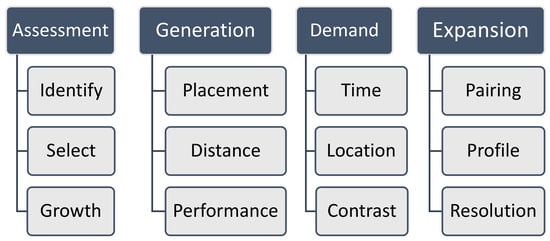
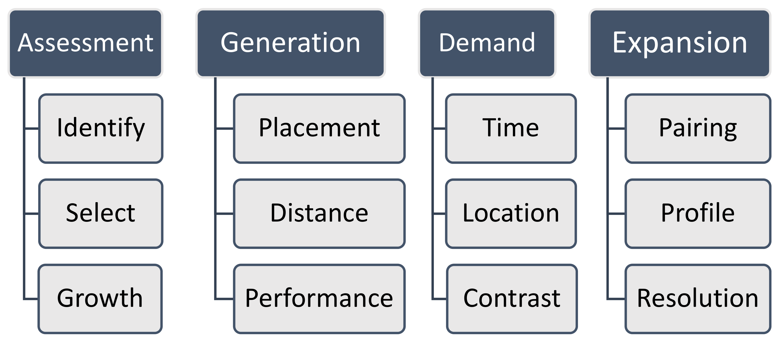
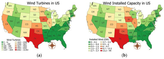
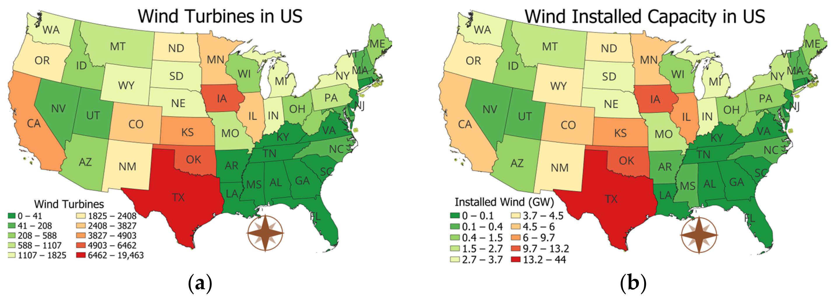
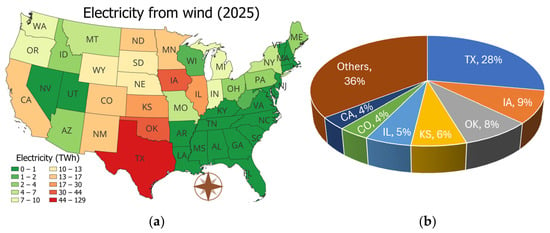
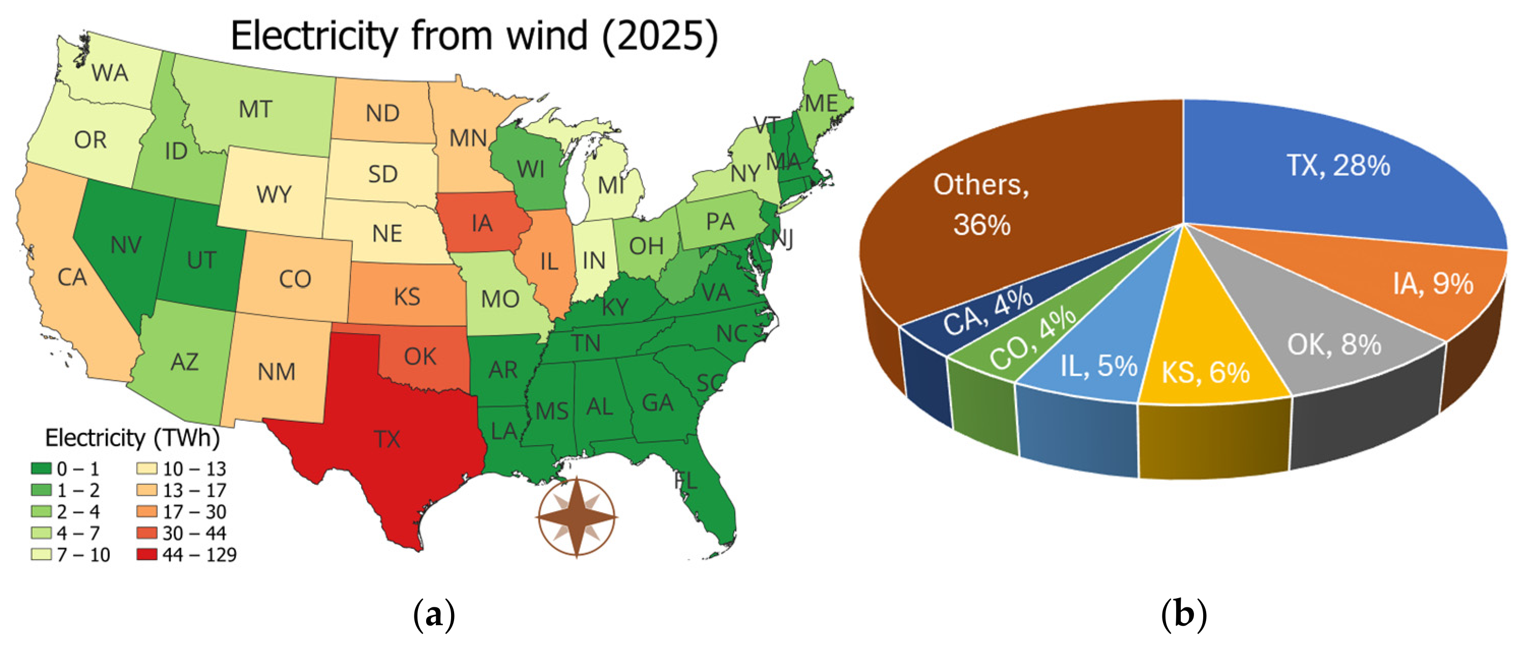
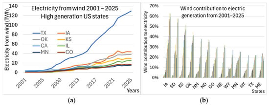
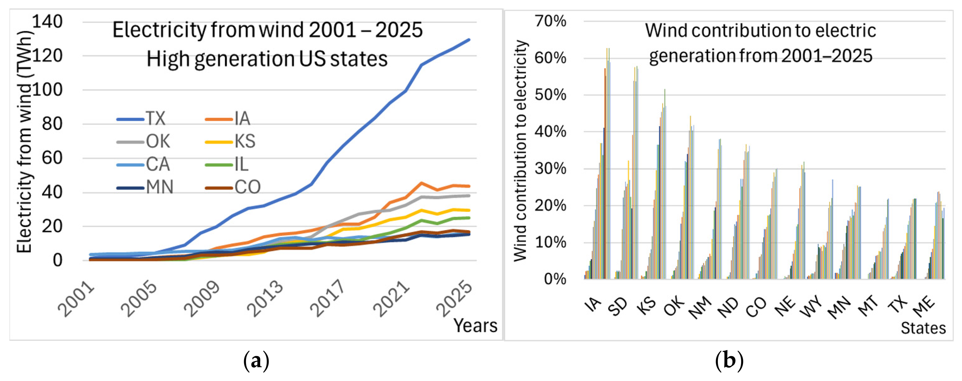
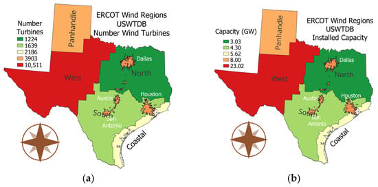
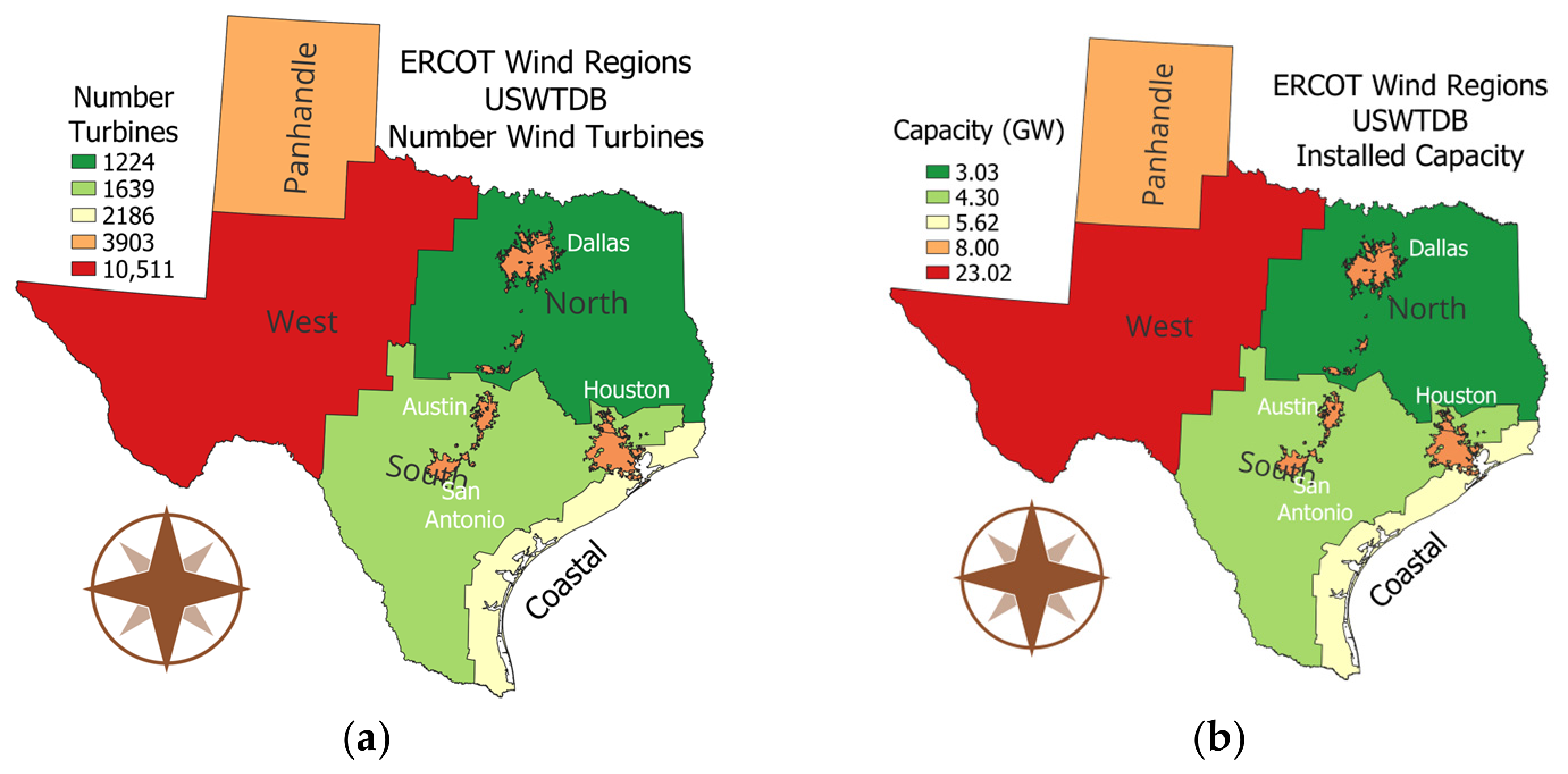
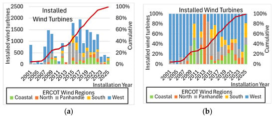
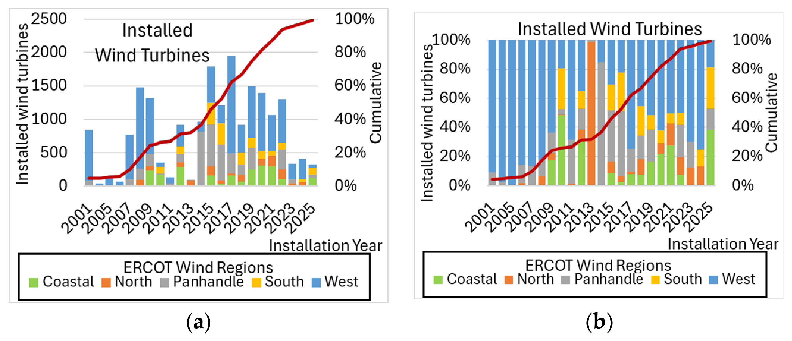
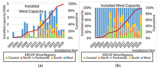
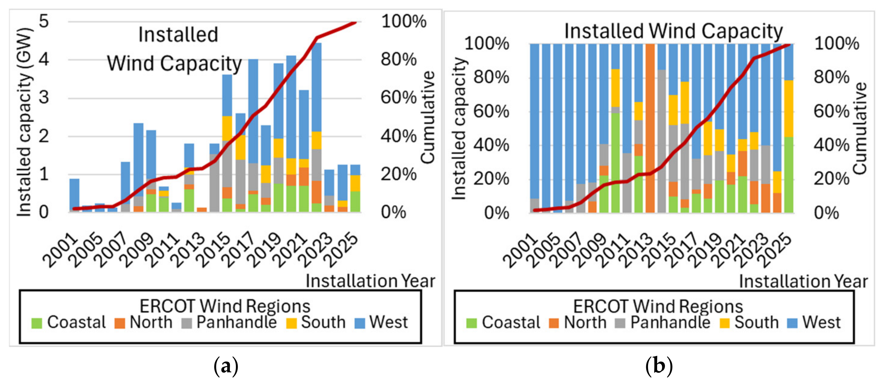
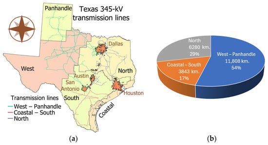
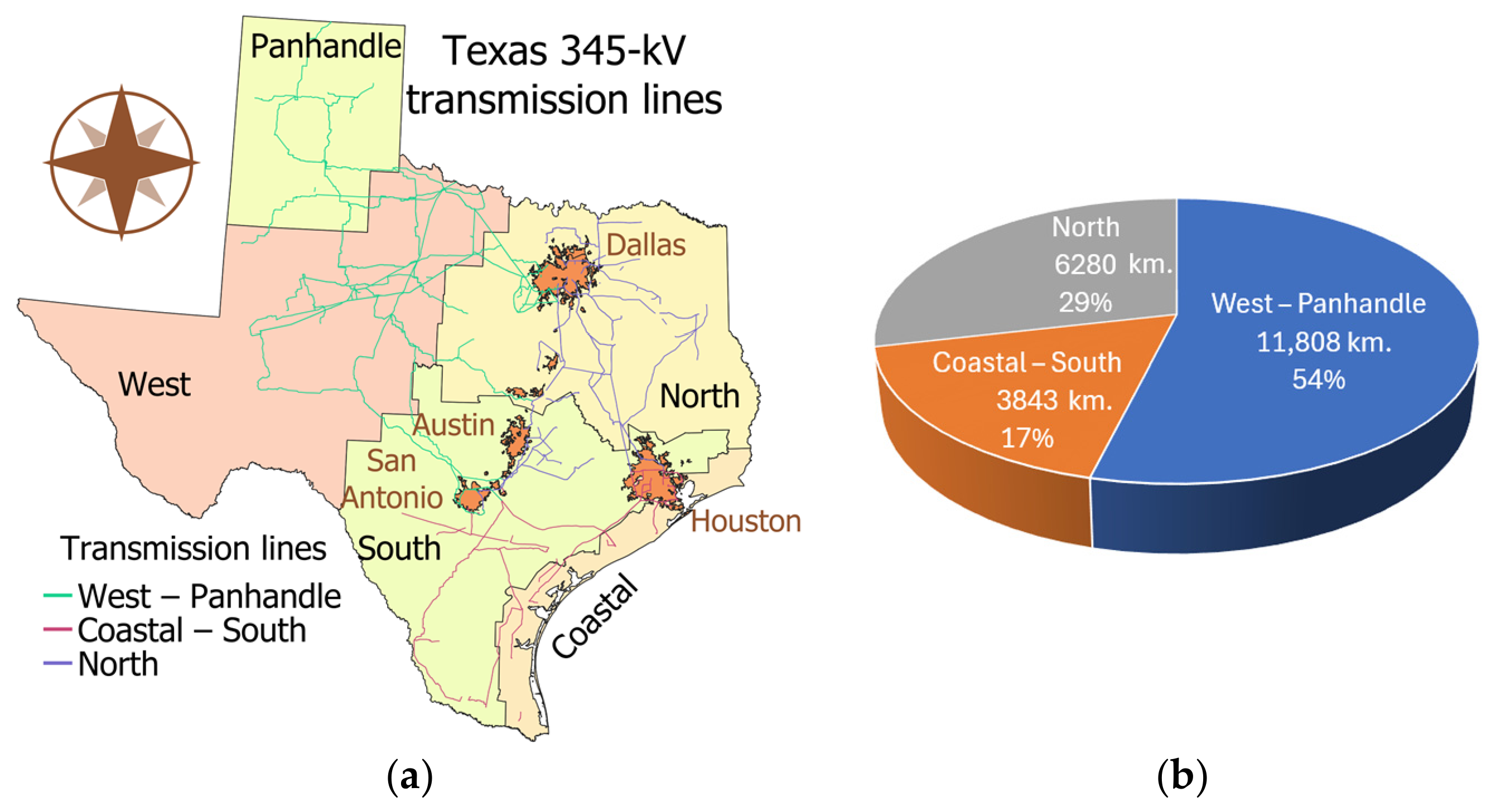
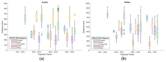
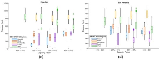
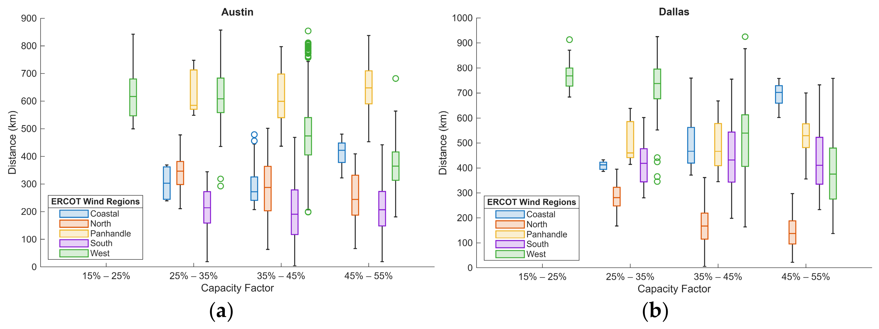
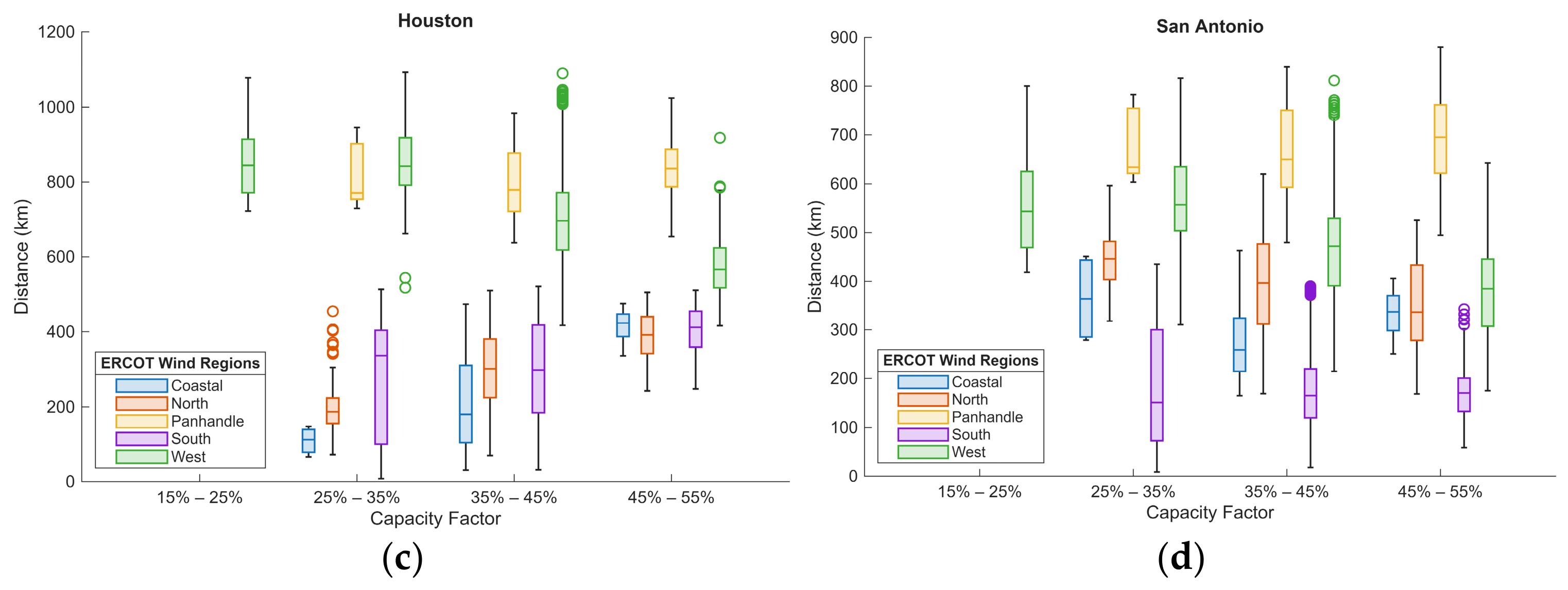
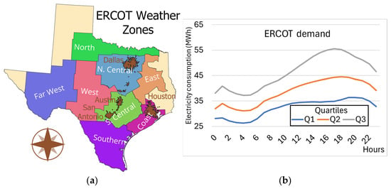
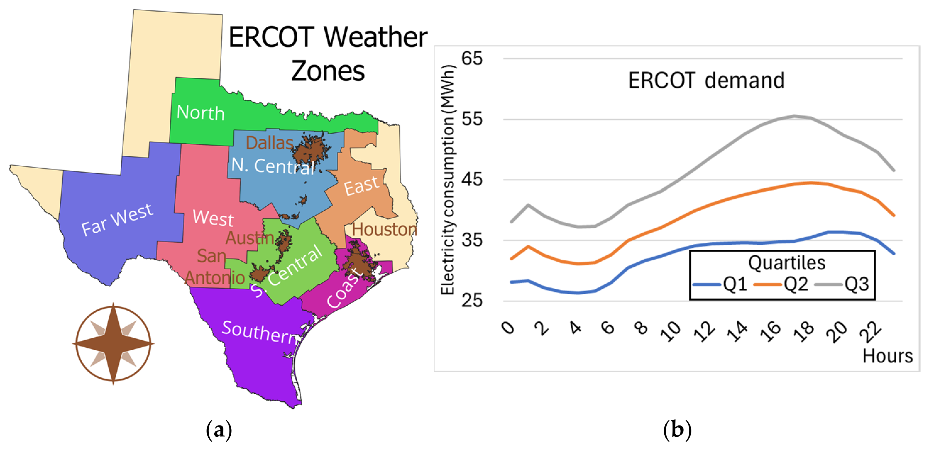
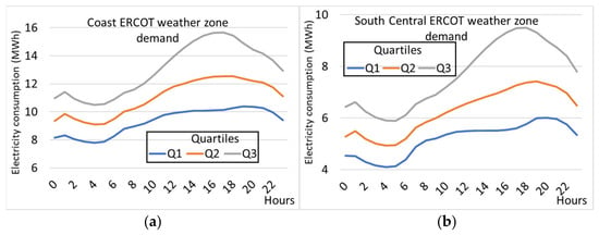
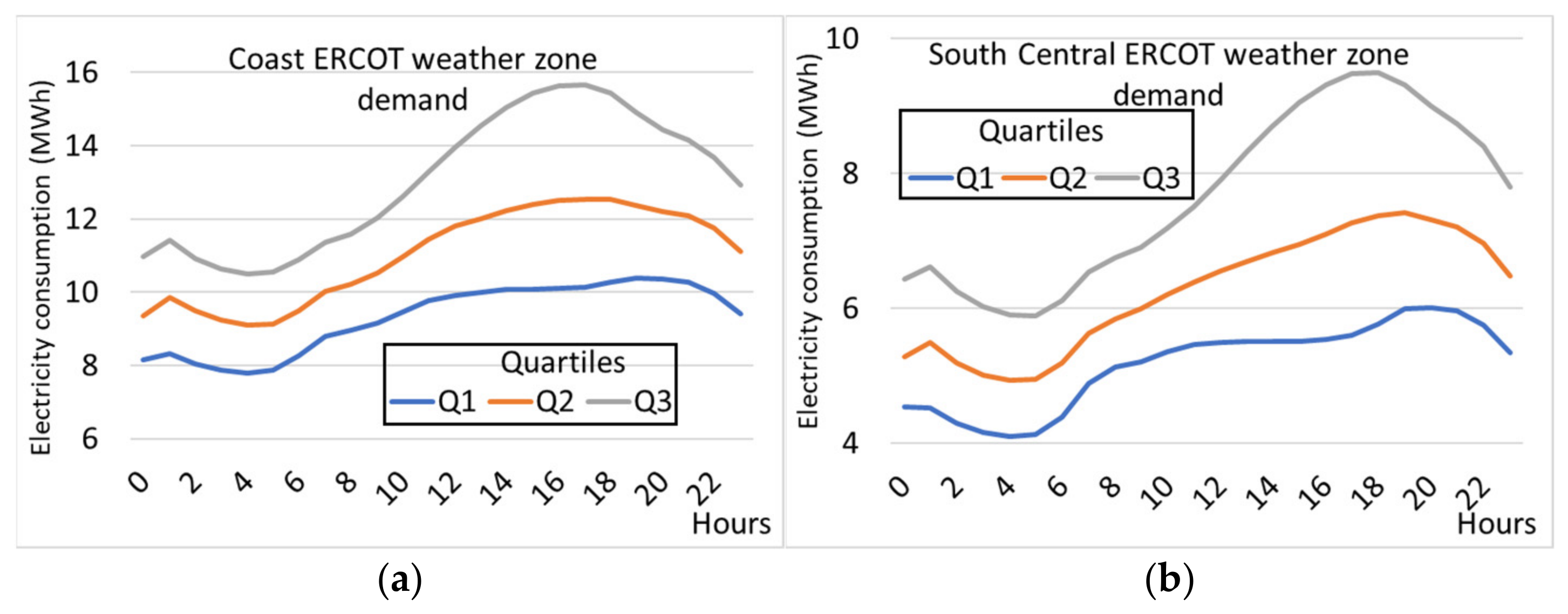
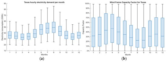
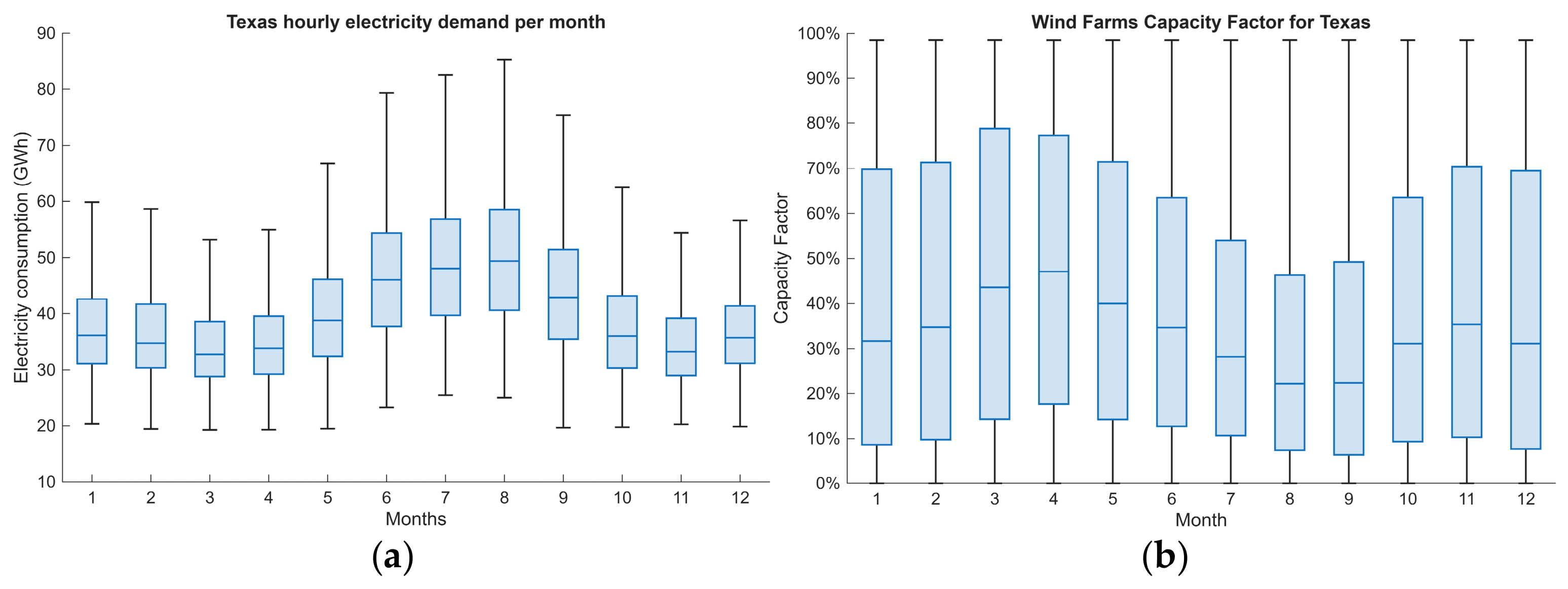
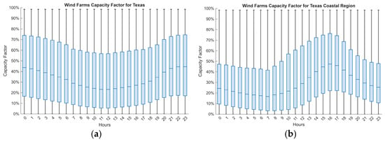
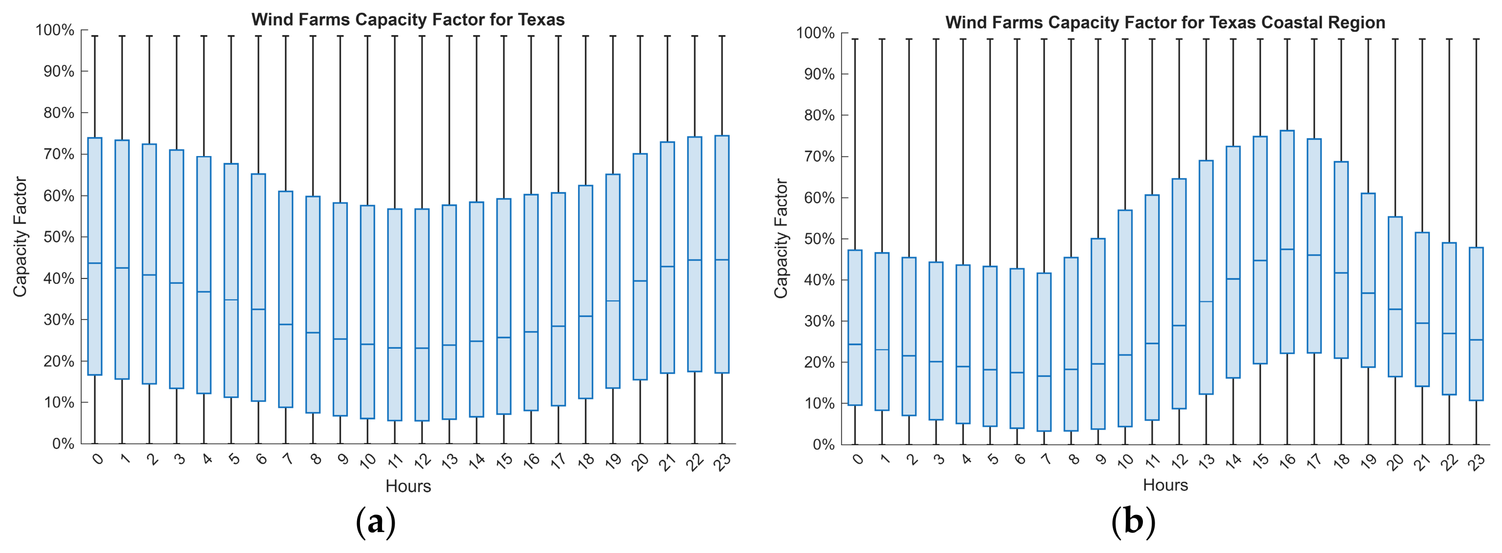
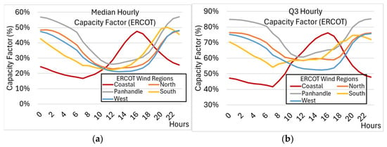
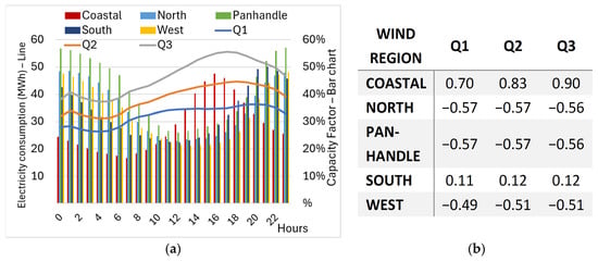
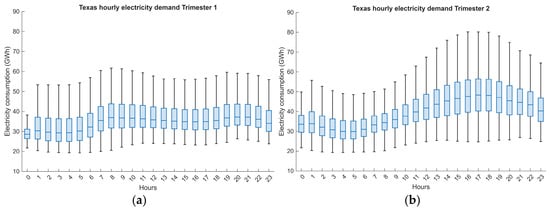
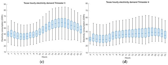
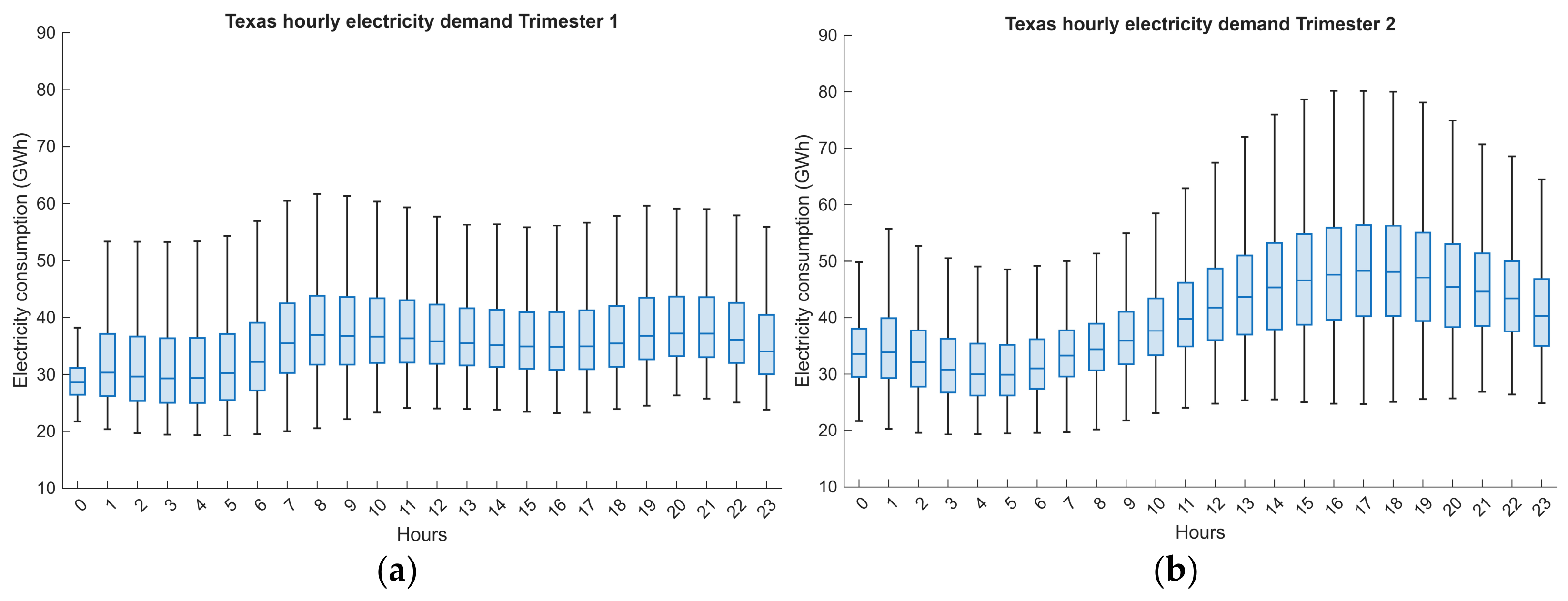
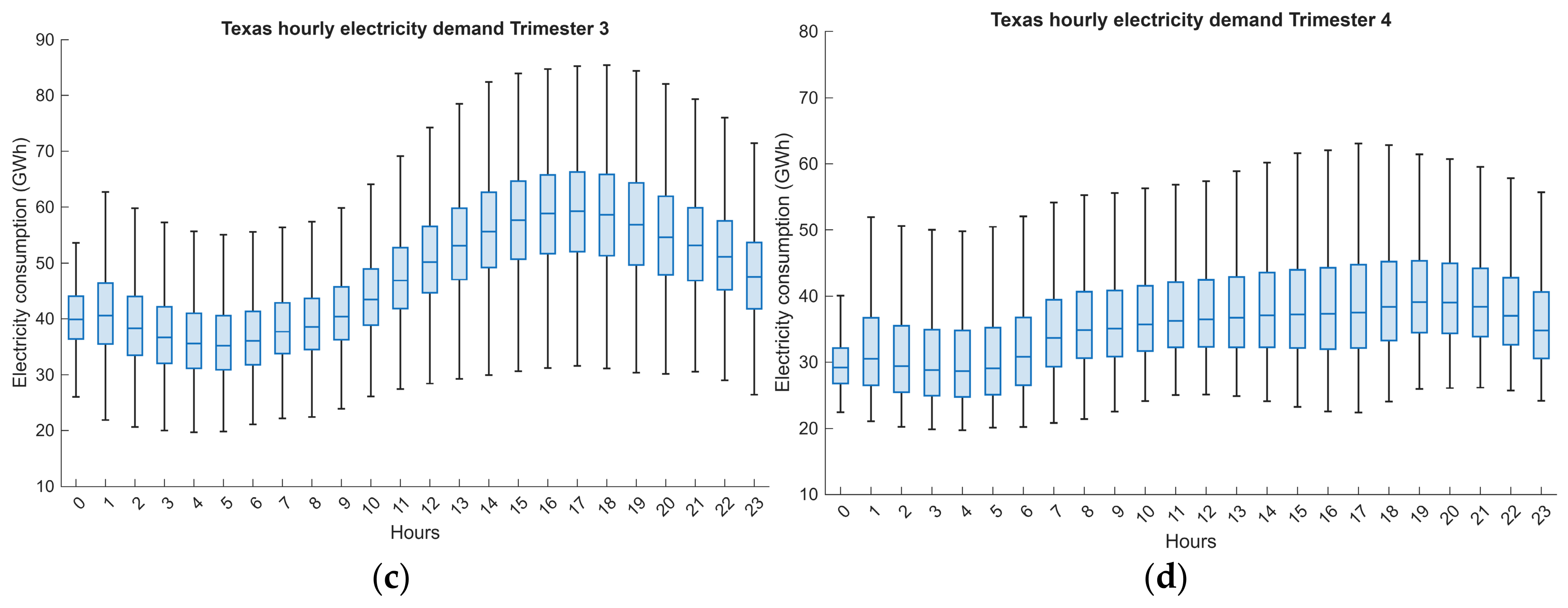
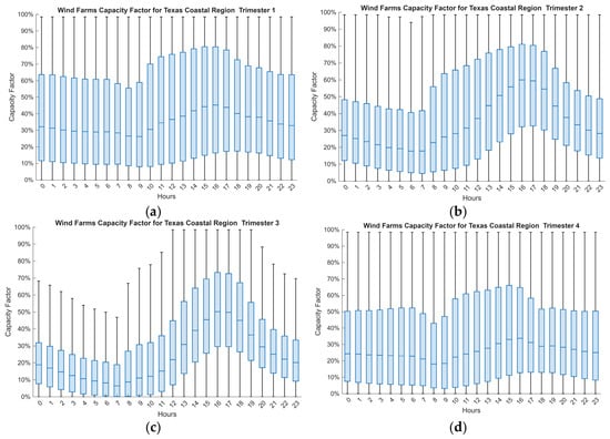
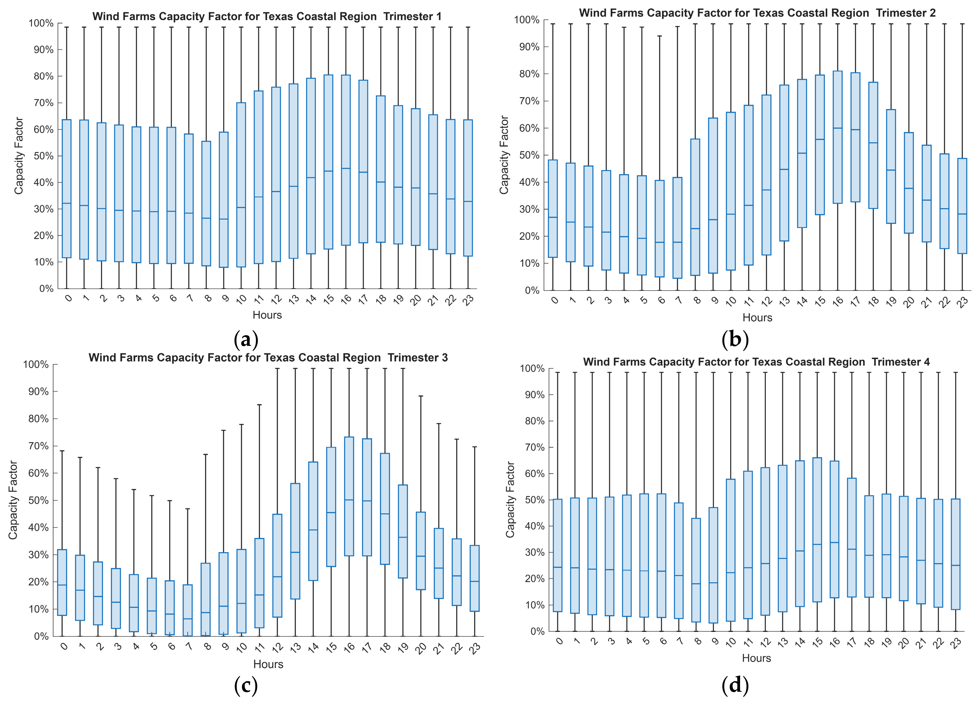
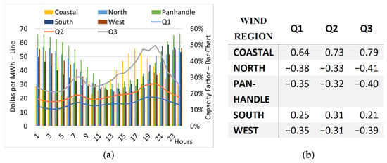
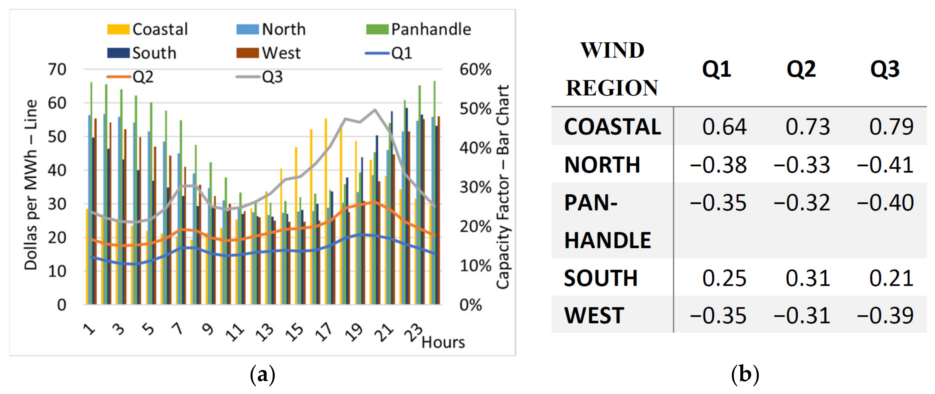
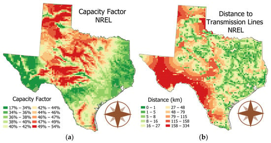
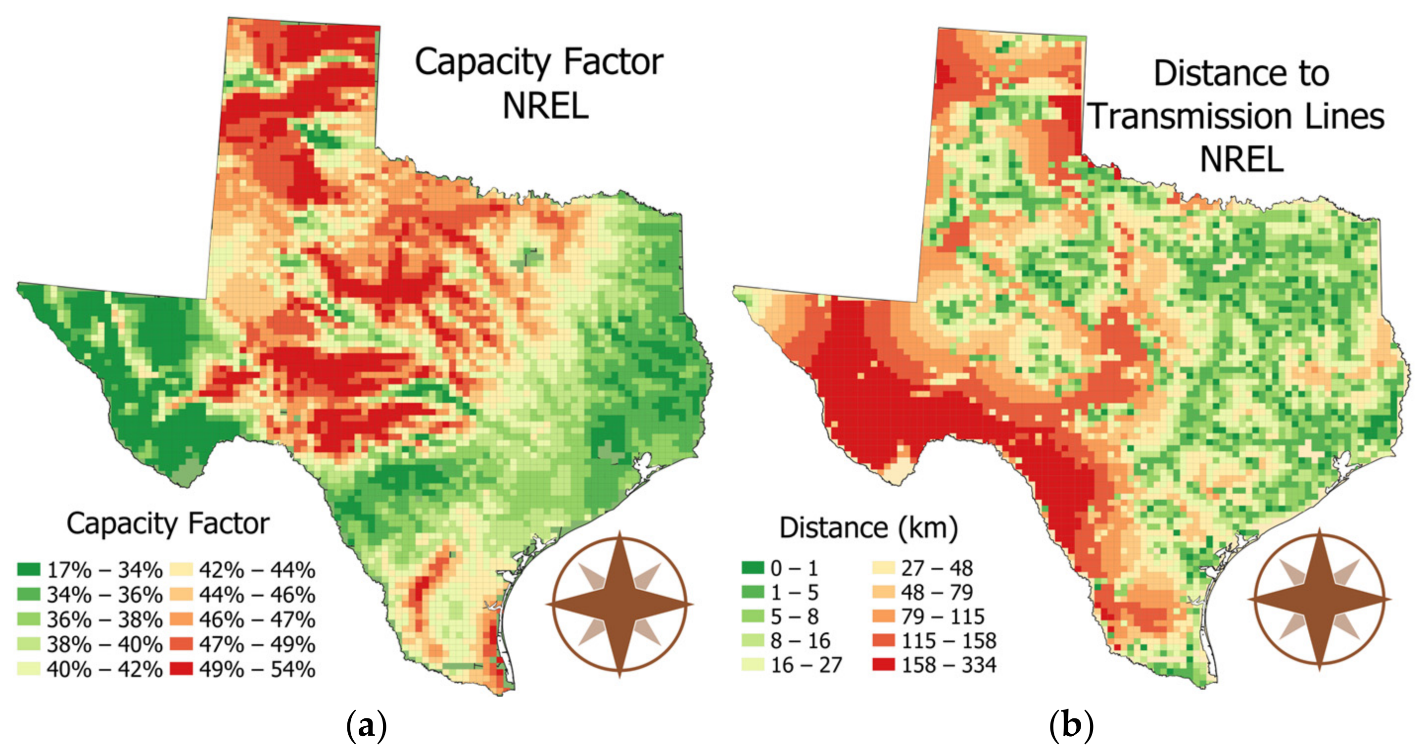
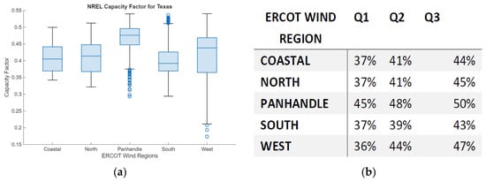
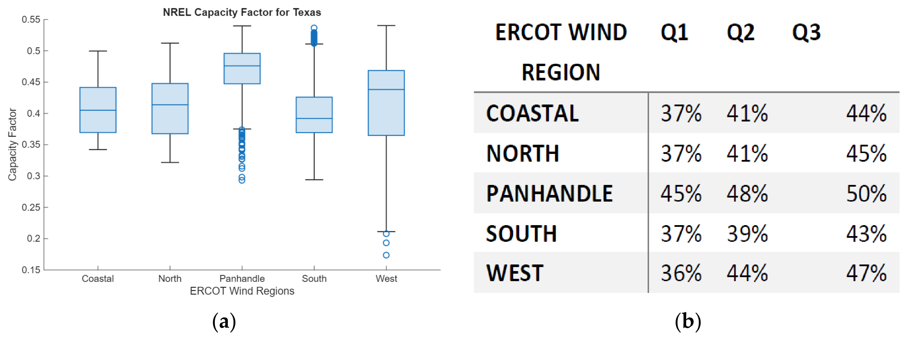
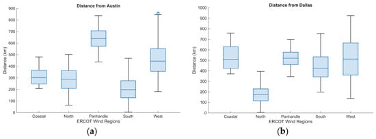
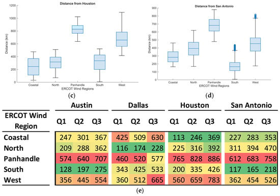
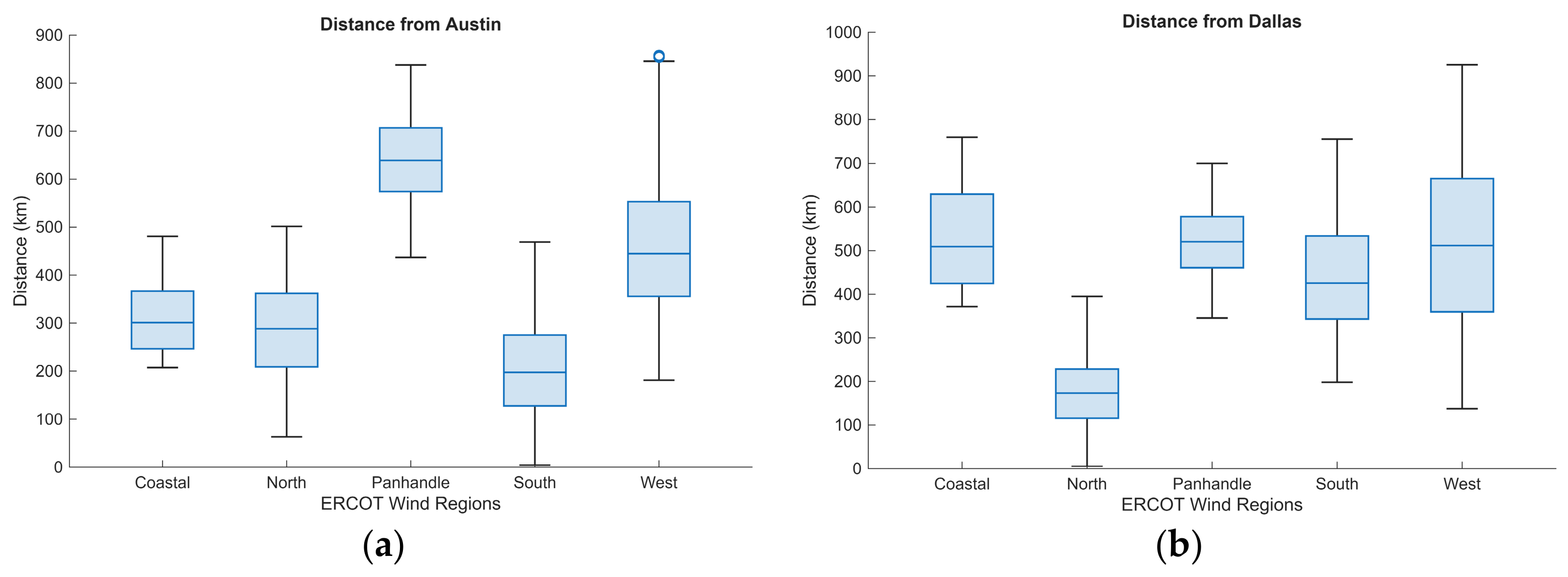
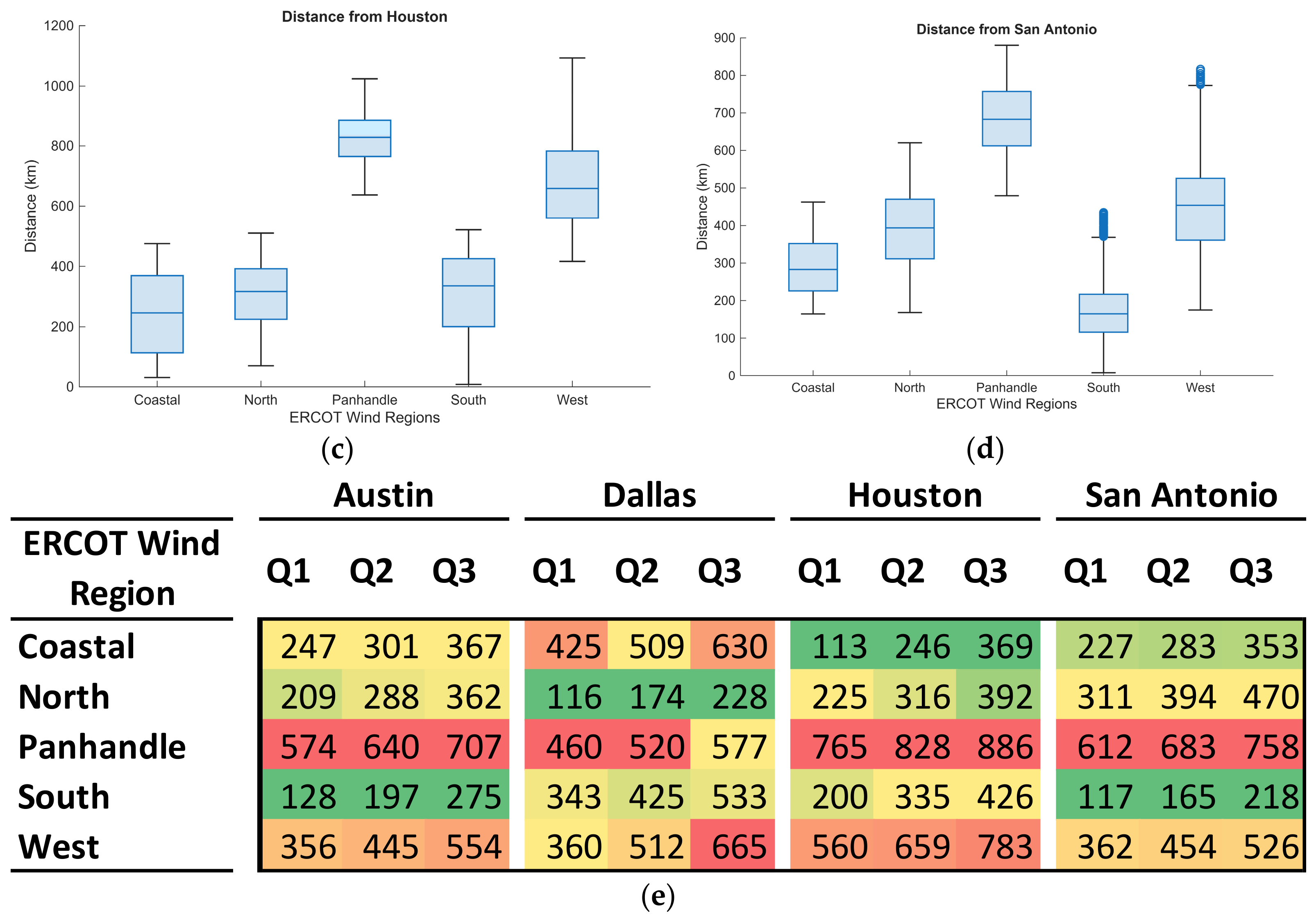
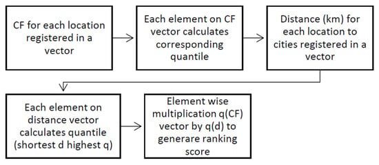
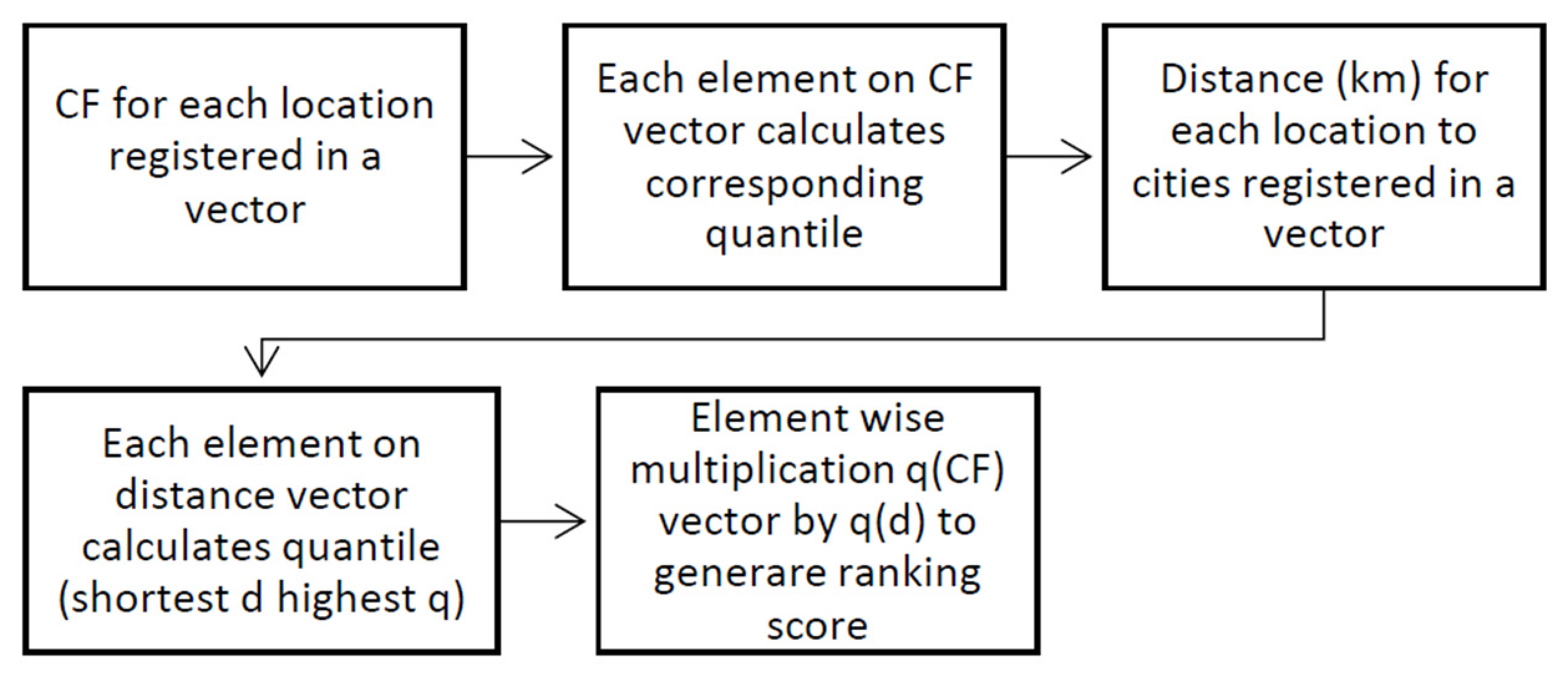
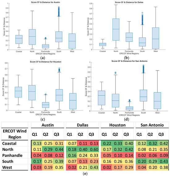
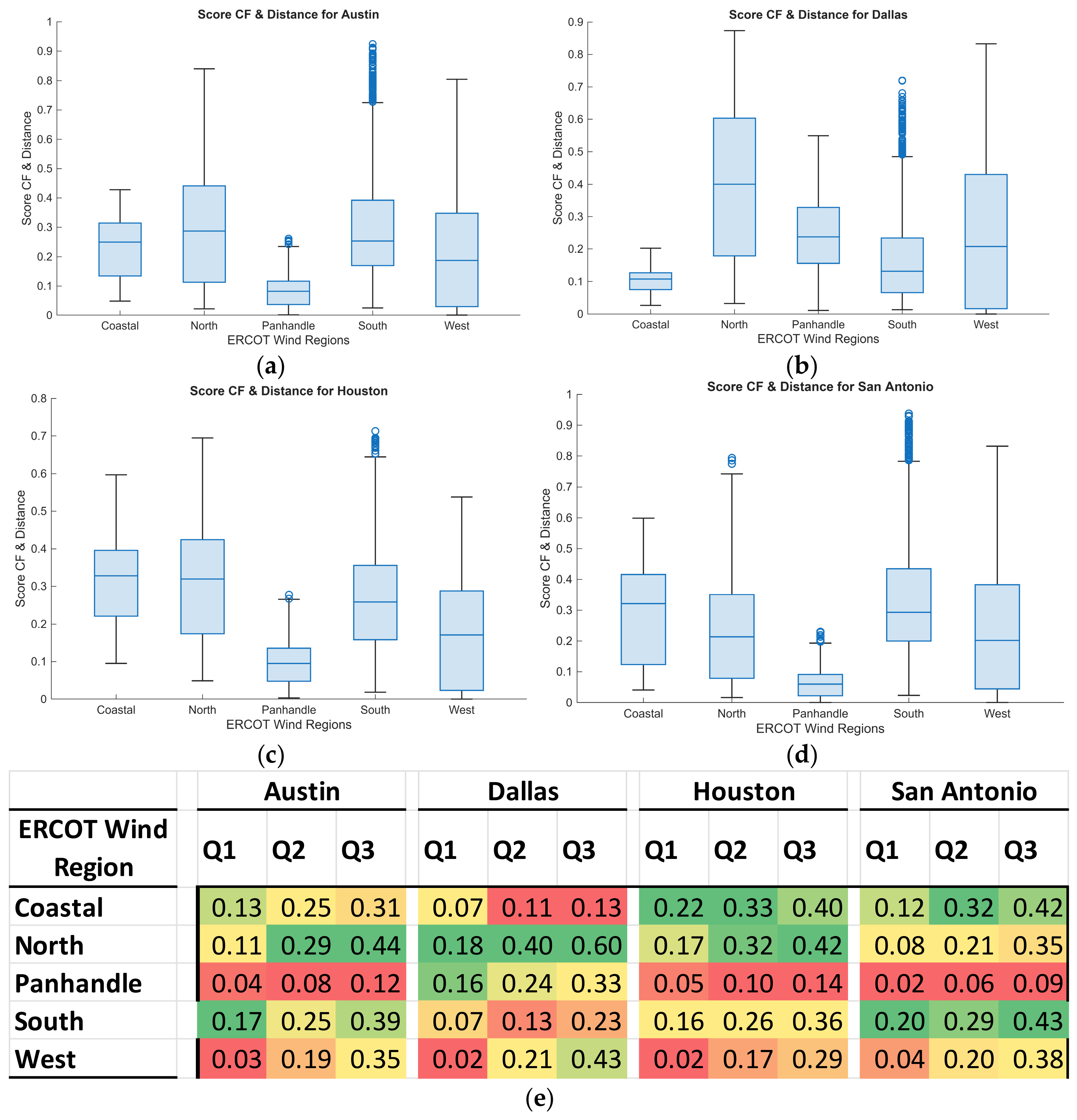
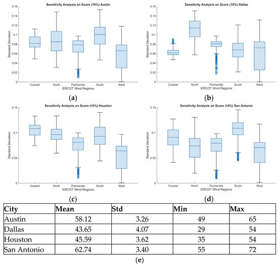
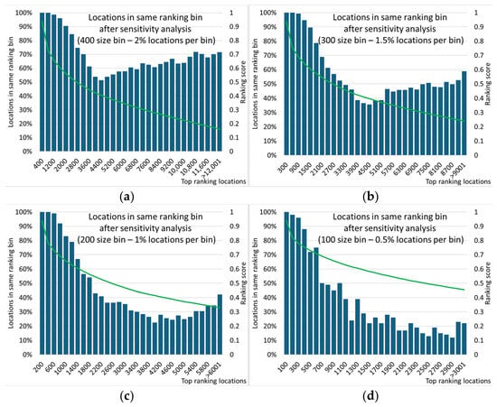
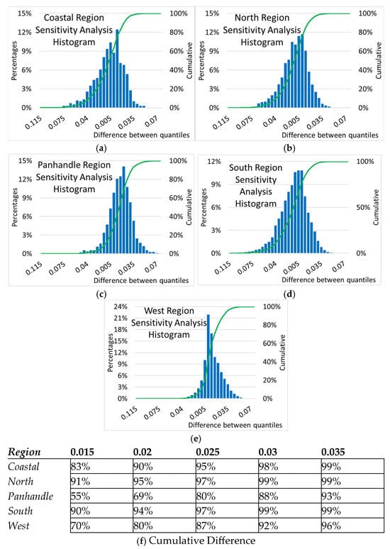
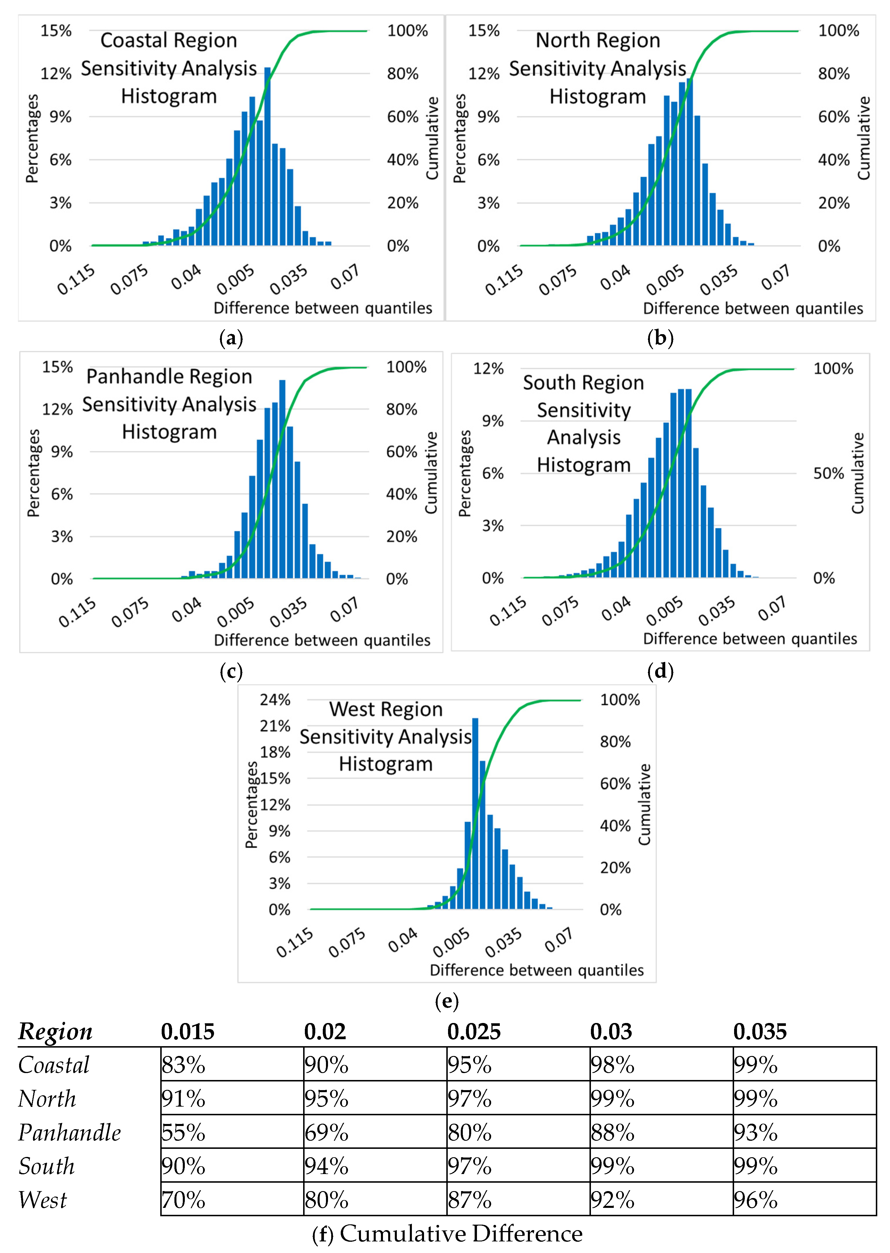
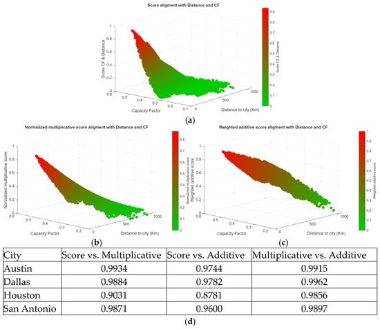
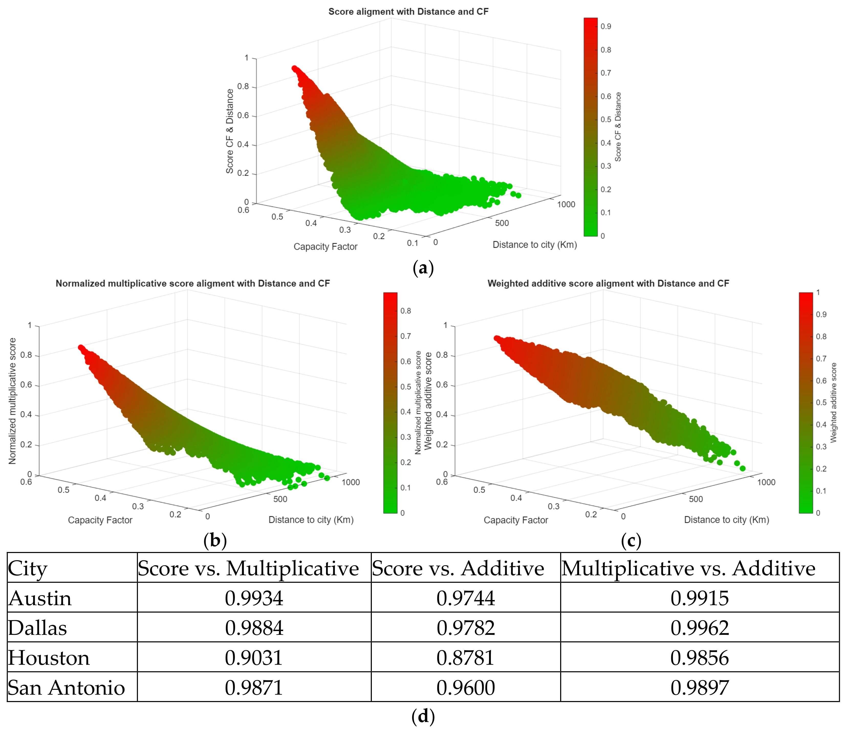
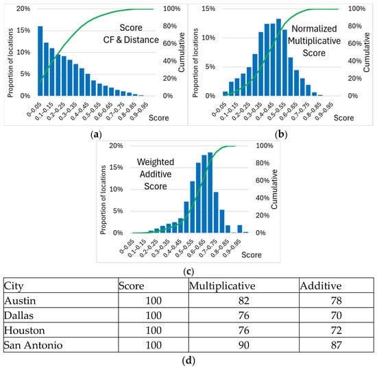
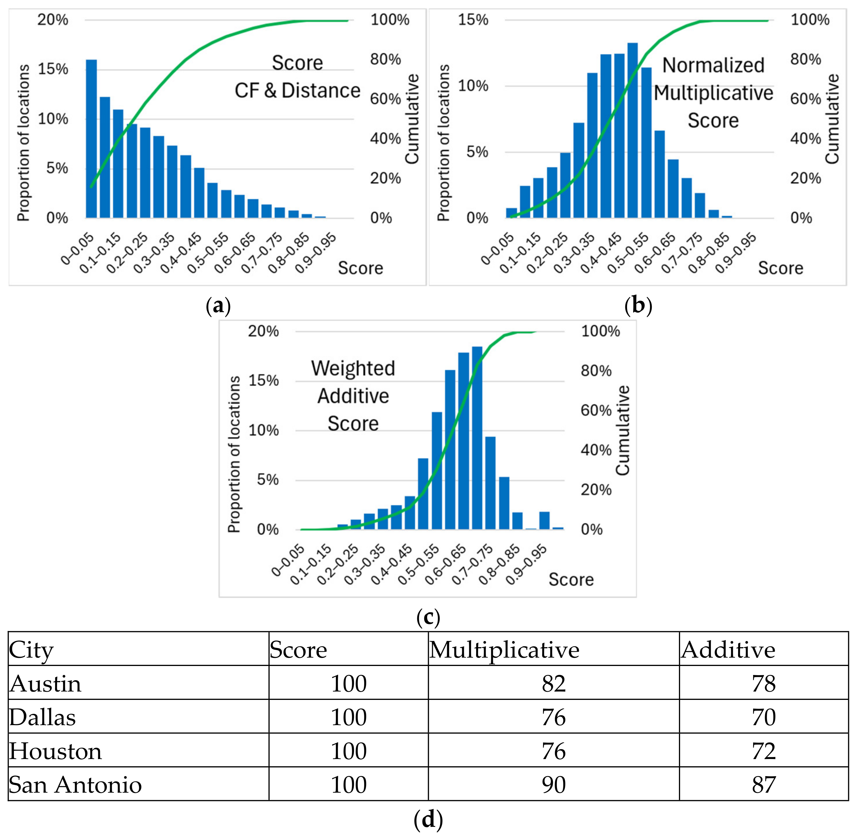
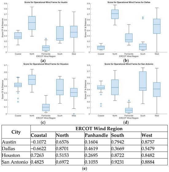
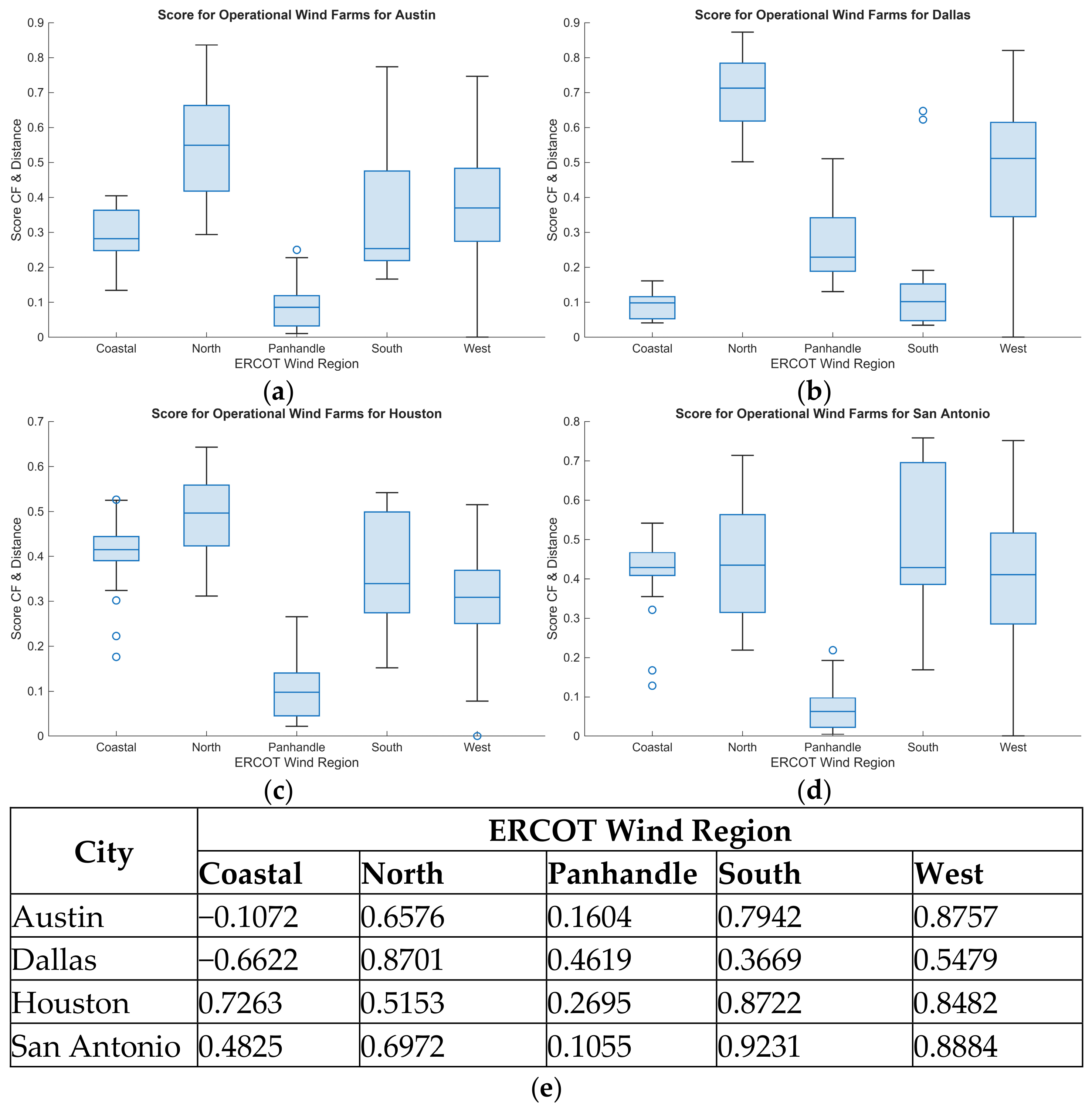
Disclaimer/Publisher’s Note: The statements, opinions and data contained in all publications are solely those of the individual author(s) and contributor(s) and not of MDPI and/or the editor(s). MDPI and/or the editor(s) disclaim responsibility for any injury to people or property resulting from any ideas, methods, instructions or products referred to in the content. |
© 2026 by the author. Licensee MDPI, Basel, Switzerland. This article is an open access article distributed under the terms and conditions of the Creative Commons Attribution (CC BY) license.