


Abstract
Background: Equitable access to public activity facilities for children and adolescents is an important dimension of social sustainability and sustainable urban mobility, yet evaluations based on static distance or a single travel mode may misrepresent service opportunities. Methods: Using Wuhan as a case study, we constructed 600 stratified community demand points representing approximately 1.90 million residents aged 5–19 years and evaluated 180 facilities. Baidu Maps navigation times for walking, weekday after-school door-to-door public transit, and driving were incorporated into a truncated Gaussian two-step floating catchment area model. Population-weighted coverage, inequality, spatial clustering, and supply–demand mismatch were assessed, with sensitivity tests for supply weights, age composition, demand definition, and route-time uncertainty. Results: Within 30 min, population-weighted coverage was 37.85% for walking, 28.44% for public transit, and 94.20% for driving. Wider time thresholds reduced weighted Gini coefficients but did not eliminate positive spatial clustering. Under the 60 min public-transit scenario, four peripheral districts contained 78.00% of the high-demand–low-service proxy population; their combined share remained 80.34% when demand was defined by population density, although classification of individual units changed. Accessibility rankings were stable under supply-weight and age-group sensitivity tests, while repeated driving observations revealed threshold-crossing uncertainty. Conclusions: Broad driving coverage cannot substitute for neighborhood-scale walking and public-transit opportunities. The framework provides an auditable tool for monitoring the spatial inclusiveness of public services and identifying priorities for facility infill and first/last-mile improvements, thereby supporting socially sustainable urban planning. The results represent potential service opportunities rather than actual travel behavior, facility use, or a comprehensive assessment of social equity.
1. Introduction
Spatial accessibility describes the possibility for individuals to obtain opportunities under the joint constraints of land use and transport impedance, and it is a core analytical concept linking public service provision with transport systems [1,2,3]. For children and adolescents, the presence of a facility on a map does not mean that it can be reached within an acceptable time: facility supply, residential demand, transport networks, and available travel modes jointly determine their potential service opportunities. Public facilities such as libraries and reading spaces, museums and cultural venues, science outreach facilities, public sports facilities, and youth activity facilities provide public activity opportunities for extracurricular reading, science learning, sports, and cultural practice. How these opportunities are distributed within a city is the first question that an evaluation of public service provision needs to answer.
This distribution is also a question of sustainability. Social sustainability concerns whether all residents, including children and adolescents, can obtain basic public services and urban opportunities in an inclusive and equitable manner [3,4,5], and sustainable urban mobility concerns whether such opportunities can be reached by walking and public transit rather than depending on private cars [6,7,8]. Children and adolescents generally cannot drive and rely on neighborhood-scale and non-car travel modes for independent access, so facilities that are reachable only by car offer them limited real opportunity and at the same time encourage car-dependent escorted trips. Spatially inclusive access to public activity facilities through walking and public transit is therefore an important component of both social sustainability and sustainable urban mobility. Defining, quantifying, and monitoring this dimension requires indicators that are reproducible and comparable across travel modes, which is the perspective adopted in this study. At the same time, the boundary of this perspective should be stated clearly: this study does not measure carbon emissions, economic costs, actual travel behavior, or the full range of social equity, and it does not attempt a comprehensive sustainability assessment; it quantifies and monitors one measurable dimension of social sustainability, namely the spatial inclusiveness of public services and the non-car service opportunities available to children and adolescents.
The two-step floating catchment area (2SFCA) method and its improved variants have been widely used to evaluate healthcare, park, educational, and cultural facilities [9,10,11], but three limitations remain when they are applied to public activity facilities for children and adolescents. First, impedance is often measured by straight-line or static network distance, which cannot adequately reflect the access, waiting, and transfer times involved in door-to-door public transit [12,13,14]. Second, most studies focus on a single travel mode or a single facility type, and few compare the gradient of service opportunities offered by the same facility system under different modes [15,16,17]. Third, results are often expressed as demand-point count ratios or regional means, which makes it difficult to present population-weighted coverage and inequality, as well as local spatial clustering corrected for multiple testing [18,19]. In addition, although navigation times derived from map APIs are closer to actual network conditions, they vary with query time, and this uncertainty has rarely been reported as a separate analytical component [20,21,22].
Wuhan has a polycentric urban structure divided by rivers and interspersed with lakes. Some supply and demand points that are spatially close to each other may have to be connected via river crossings or routes around lakes, so that straight-line distance and navigation time may diverge considerably; this makes Wuhan a suitable case for testing multimodal navigation-time measures. Previous studies in Wuhan have separately identified spatial disparities in educational services and youth-park accessibility [23,24], but no study has yet jointly evaluated multiple types of public facilities—cultural, sports, science and technology, library, and youth activity facilities—into a single framework and combines age-specific population, door-to-door public transit, and population-weighted indicators.
To address these gaps, this study develops a multimodal truncated Gaussian two-step floating catchment area framework. The sum of the population aged 5–19 years in the WorldPop 2025 age-structured rasters is used to represent proxy demand, addressing the inability of demand-point counts to reflect population competition. A total of 600 standardized community demand points covering 170 “district × subdistrict/town” strata in the 13 districts are used to represent potential service opportunities from places of residence, maintaining spatial representativeness under API cost constraints. Walking, metro-priority door-to-door public transit, and driving times reflecting traffic conditions at the time of query are obtained from the Baidu Maps Web API, addressing the limitations of static distance and single-mode analysis. In terms of indicators, we simultaneously report the population-weighted reachable population share, the weighted Gini coefficient, global Moran’s I, and false-discovery-rate (FDR)-corrected local indicators of spatial association (LISA); in terms of robustness, we test the conclusions through supply-weight perturbation, recalculation by age group, same-origin–destination (OD) comparisons across time periods, and repeated observations.
This study addresses four research questions. RQ1: How do the coverage and inequality of the potential service opportunities available to the proxy demand population of children and adolescents vary across travel modes and time thresholds? This question is answered using the population-weighted reachable population share and the weighted Gini coefficient. RQ2: Are service opportunities significantly spatially clustered, and are the conclusions robust to the specification of spatial weights? This is answered using global Moran’s I with k = 4,8,12 and FDR-corrected LISA. RQ3: What differences in resource allocation exist between district-level facility provision and the proxy demand population, and where are high-demand–low-service units concentrated? This is answered using count-based location quotients (LQs), weighted-supply LQs, and a four-type supply–demand classification. RQ4: Are these patterns robust to uncertainty in supply weights, the age composition of the population, and route-time impedance? This is answered using 1000 Monte Carlo perturbations within ±20%, recalculation by age group, same-OD comparisons across time periods, and repeated observations.
This study makes three contributions. Methodologically, it integrates door-to-door multimodal navigation time, population-weighted equality indicators, and tests of route impedance uncertainty into a single auditable workflow, and it explicitly distinguishes the main citywide G2SFCA scenarios from the sensitivity samples. Empirically, it provides evidence on differences in the potential service opportunities of public activity facilities for children and adolescents in Wuhan across travel modes, time thresholds, and spatial distribution, thereby providing a basis for identifying areas with weak service opportunities. From a sustainability perspective, the framework provides a reproducible tool for monitoring the spatial inclusiveness of public service provision for children and adolescents and the extent to which these services can be reached by non-car travel modes, which corresponds to one measurable dimension of social sustainability and sustainable urban mobility. This study measures potential service opportunities from places of residence and their spatial distribution: demand points do not represent the actual travel origins of individuals, and Ai does not represent facility utilization or satisfaction. Because information on income, car ownership, and travel diaries is not included, the conclusions are limited to spatial equality and differences in resource allocation and do not constitute a comprehensive social-equity or causal judgment.
2. Literature Review
Starting from the opportunity–impedance relationship, spatial accessibility research has gradually developed into an evaluation framework that simultaneously considers land use, transport costs, and the distribution of opportunities [1,2]; research on distributive justice in transport has further shifted attention to differences in access to opportunities among population groups [3]. Empirical studies have covered public sports facilities [25], educational facilities [26,27], cultural and comprehensive public facilities [28,29,30], as well as healthcare and park services [11,31,32]. These studies show that supply scale, population competition, and analytical scale jointly affect judgments of spatial equality. In this article, spatial equity denotes the broader planning objective, whereas spatial equality is the distributive dimension operationalized through the relative spatial distribution of the proxy demand population and potential service opportunities. This operational measure is neither a mechanical averaging of facilities nor a comprehensive assessment of social equity that controls for differences in income, car ownership, and individual capabilities. Around the questions of “how to measure” and “what the measurement results can show,” existing research involves at least the following five debates.
2.1. Static Distance Versus Navigation Time
Early 2SFCA studies mostly defined service areas by straight-line or network distance [33,34]. This approach offers computational transparency and reproducibility, but it cannot adequately reflect access, waiting, and transfer times in public transit or temporal variations caused by road congestion. Map-service APIs and public transit network data have made navigation-time-based measurement possible [20,21,22], and reviews have regarded multimodal transport and spatiotemporal disaggregation as important advances in accessibility measurement [14]. However, navigation times are returned by an API at a specific query time; while they incorporate useful information such as real-time traffic conditions, they also introduce new uncertainties, including dependence on query time and opaque API rules. Therefore, once navigation times are adopted, the sensitivity of the measurement results to query periods and repeated queries should be tested as part of the method itself, rather than assuming by default that navigation time is the “true” impedance.
2.2. Single-Mode Versus Multimodal Measurement
Single-mode evaluation implicitly assumes that all members of the demand population use the same travel mode. Multimodal 2SFCA studies have shown that switching among walking, public transit, and driving markedly changes the reachable range and spatial pattern of parks, hospitals, and job opportunities [11,15,16,21]; extensions that consider facility perception and mode choice further show that both the supply proxy and the mode specification affect the results [17]. In terms of presentation, multimodal measures can either be combined into a single index according to mode shares or reported separately by mode. The former depends on reliable mode-share data, whereas the latter better preserves the gradient of service opportunities across modes when travel survey data are lacking. For children and adolescents, driving depends on an available vehicle and driver, whereas walking and public transit relate more directly to their non-driving travel conditions; mode-specific comparison is therefore particularly informative.
2.3. Demand-Point Counts Versus Population Weighting
Summarizing coverage as “number of reachable demand points/total number of demand points” or as regional means is intuitive when demand points have similar population sizes; however, when the populations of demand units differ substantially, this approach confuses “how many places are served” with “how many people are served.” The 2SFCA method introduces population competition through the supply–demand ratio [33,34], and equality studies often use population-weighted coverage, the Gini coefficient, and Lorenz curves to shift the object of evaluation from places to people [10,18,19]. The source of the demand population also involves trade-offs: registered community populations rarely provide a uniform and complete age structure; estimation from household counts and a uniform age proportion smooths away spatial differences in age composition; and open gridded population data provide reproducible age-group data but are model estimates that must be clearly distinguished from registered population.
2.4. Hard Thresholds Versus Continuous Decay
The conventional 2SFCA assigns equal weights within the threshold and zero beyond it, causing abrupt changes in service opportunities on either side of the boundary [33,34]. The enhanced 2SFCA mitigates this problem through stepwise weights [35], whereas Gaussian functions and their modified forms represent within-threshold distance decay through continuous decay [15,36,37]. The debate concerns what the threshold and decay parameters actually represent. If they are regarded as behavioral regularities, they require support from travel surveys; if they are regarded as analytical settings, the robustness of the conclusions should be tested by comparing multiple thresholds. In the absence of travel surveys of children and adolescents, the latter approach is more prudent: thresholds are used to compare how service opportunities respond to the expansion of time budgets, without claiming that any particular number of minutes is a hard boundary of acceptable travel for children and adolescents [7,19].
2.5. Potential Accessibility Versus Actual Behavior
Accessibility measures the potential to obtain opportunities, which differs from actual use. Research on children and adolescents shows that independent mobility, activity origins, accompaniment conditions, and acceptable travel ranges all vary with age and context [6,38,39]. Chinese research has likewise moved from reviews of the built environment surrounding school travel to empirical investigation of independent mobility, highlighting the joint roles of residential, school, and broader urban environments [8,40]. Studies that improve G2SFCA using travel-behavior parameters [18] and those that incorporate facility perception [17] have both attempted to narrow this gap. Research on child-inclusive public spaces further emphasizes that spatial proximity does not equate to sustained access and use [4,5]. Studies of youth parks in Wuhan, community children’s spaces in Hangzhou, and children’s parks in Changsha show that facility layout and travel constraints jointly shape differences in service opportunities [24,41,42]. This implies that, in the absence of travel diaries and usage data, the results of accessibility models can only be interpreted as potential service opportunities and cannot be directly equated with utilization or welfare levels.
2.6. Research Gaps and Positioning of This Study
Within the Chinese-language literature, studies have examined community-scale accessibility of children’s education, healthcare, and recreation facilities, as well as interurban differences in the allocation of children’s public services [43,44]. Taken together, existing research leaves room for extension in three respects. First, studies of facilities for children and adolescents mostly focus on parks, green spaces, or community children’s spaces [24,38,41], and few incorporate multiple types of public facilities—such as libraries, museums and cultural venues, science outreach, sports, and youth activity facilities—into a single framework. Second, multimodal studies rarely report population-weighted coverage, inequality, and local clustering corrected for multiple testing at the same time. Third, the time-of-day dependence of navigation times and fluctuations across repeated queries have rarely been reported as a separate component of uncertainty. Accordingly, this study adopts mode-specific comparison, population-weighted indicators, truncated Gaussian decay under nested thresholds, and route sensitivity tests, and it limits its conclusions to the spatial equality of potential service opportunities.
3. Data and Methods
3.1. Study Area and Analytical Units
Figure 1 summarizes the research workflow. The study area comprises the 13 administrative districts of Wuhan. The candidate demand-point pool came from the public community directory of the Wuhan Municipal Civil Affairs Bureau [45] and contained 1454 records with 1382 unique coordinates. We stratified the pool by administrative district and standardized subdistrict/town. District quotas were allocated by the Hamilton largest-remainder method according to the available candidates, with at least one point retained in every ‘district × subdistrict/town’ stratum. Within each stratum, the mean distance to the eight nearest neighbors served as a residential-density proxy, and a quality-first deterministic max–min distance algorithm selected 600 points. The fixed seed 20251006 generated a stable hash used only to break otherwise tied selection scores, so the procedure remained deterministic and reproducible. The final sample covers 13 districts and 170 eligible subdistrict/town groups, contains no duplicate coordinates, and increases the median nearest-neighbor distance from 0.372 km in the candidate pool to 0.732 km. Each demand point and proxy demand area represents potential service opportunities from places of residence rather than an observed individual origin or realized trip.
Figure 1.
Research workflow of this study.
Using 600 points rather than all 1382 unique coordinates balanced API-call costs and spatial representativeness. Using every coordinate as an origin would have greatly increased the number of OD combinations across the three modes and exceeded the available API quota (Appendix A, Table A1), whereas unrestricted random sampling could have overrepresented community-dense central districts. The stratified max–min design reduced the sample size while preserving coverage and increasing spatial dispersion.
3.2. Data Sources and Quality Control
Table 1 summarizes the data sources and processing, and Figure 2 maps the demand units, proxy population, and facility sample. Population data came from the WorldPop 2025 R2025A v1 constrained age-structured rasters at approximately 1 km resolution (WGS84) [46], and the population aged 5–19 years was calculated strictly as P5−19 = P5−9 + P10−14 + P15−19. Because publicly available, complete, and directly downloadable community polygon data are lacking, the 13 district boundaries obtained from the administrative-boundary data service [47] were first used as spatial constraints; proxy subdistrict/town areas were then inferred from the 1382 candidate points in the government directory, and 600 Voronoi demand units were constructed within these proxy areas. Raster population was allocated by each cell’s intersected-area fraction, and the OD origin of each unit was taken as its P5−19 population-weighted center. This process yielded approximately 1.90 million proxy residents aged 5–19 years, a model estimate rather than registered community population.
Table 1.
Data Sources, Spatial Scales, and Variable Definitions.
Figure 2.
Spatial distribution of demand units, the population of children and adolescents, and the facility sample.
WorldPop age rasters were adopted instead of registered community population for two main reasons: first, uniform and complete community boundaries and age-specific population data are lacking in public sources; second, the rasters directly provide age groups of 5–9, 10–14, and 15–19 years, which facilitates testing the effect of age composition on the results. This choice involves three costs: the approximately 1 km raster and the Voronoi proxy demand units are inconsistent in scale; areal allocation implies an assumption of uniform population distribution within each cell; and the boundaries of the proxy units differ from actual community boundaries. Therefore, the proxy demand population is suitable for comparing relative spatial patterns within the city, but not for headcount accounting at the unit level or for direct comparison with registered population.
Table 2 summarizes quality assurance (QA) for the demand and facility samples. On the facility side, the process began with 3105 raw results returned by the Baidu Place API [48], which were merged into 1867 unique identifiers (UIDs). After facility-type pre-screening, verification against official government webpages, review of public-service attributes, and merging of duplicate points of interest (POIs), 180 eligible facilities remained. They comprise public libraries and reading facilities; museums, memorial halls, and art galleries; science outreach facilities; public sports facilities; public cultural, educational, and practice facilities; and youth/children’s activity facilities. We excluded commercial training institutions, retail stores, private or privately run institutions, on-campus facilities, facilities that were only planned or not regularly open, weakly related POIs, and POIs that could not be uniquely verified. All six facility types and all 13 districts are represented. Thirty-three facilities retain a manual-review flag because their service level or supporting evidence could not be verified with sufficient precision.
Table 2.
QA Summary of the Demand-Point and Facility Samples.
Eligibility required verifiable public-service status, target users, and operating status; this prevented raw POI counts from being treated as equivalent to public-service supply. To assess residual evidence uncertainty, we recalculated all main scenarios using the 147-facility sample obtained after excluding the 33 facilities carrying a manual-review flag (Section 4.6 and Appendix B). Analyses used Python 3.11.7 with NumPy 1.26.4, pandas 2.1.4, SciPy 1.11.4, scikit-learn 1.2.2, Shapely 2.1.2, and Matplotlib 3.8.0; no instruments or reagents were used.
3.3. Travel Modes, Behavioral Scenarios, and OD Sampling
Table 3 summarizes main-scenario OD coverage and sampling limitations. Walking used RouteMatrix Walking with thresholds of 5, 15, and 30 min. Public transit used the Baidu Transit Direction endpoint [48] with the metro-priority policy (tactics_incity = 5). T1 specified 13 October 2026 and 16:00–18:00 as the requested departure date and time window. The first recommended door-to-door route was retained, and its complete duration included access and egress walking, waiting, transfers, and in-vehicle travel. Metro priority did not exclude conventional buses: in a fixed-seed audit of 2000 valid T1 responses, every route contained metro and walking segments, 592 also contained conventional-bus segments, and none was walking-only. Driving used the standard recommended routing policy with traffic conditions at query time. The 100,127 primary D1 routes were collected during the actual 16:00–18:00 after-school window: 89,501 routes from 16:31 to 17:42 on 12 October 2026 and the remaining 10,626 routes from 16:05 to 16:15 on 13 October 2026. The citywide T1 and D1 scenarios both used thresholds of 30, 45, and 60 min.
Table 3.
Main-Scenario OD Coverage and Sampling Limitations.
Time thresholds follow a nested sensitivity design rather than treating a single threshold as a uniform behavioral limit for all children and adolescents. A 5 min walk represents immediate-proximity services, 15 min corresponds to a common planning scale for everyday neighborhood services, and 30 min is used to test changes in coverage as the walking time budget expands [7,19]. The 30, 45, and 60 min thresholds for public transit and driving are used to compare the gradient of cross-community service opportunities as the broad-area time budget expands and remain comparable with the graded time-cost treatments in multimodal accessibility studies [14,15,21]. These thresholds are used for model comparison and do not imply that all age groups between 5 and 19 years have the same independent travel capability or acceptable travel duration [6,38,39].
The route data fall into two categories: main scenarios and sensitivity samples. The main scenarios are walking W, public transit T1, and driving D1 used in the complete citywide G2SFCA calculations; all coverage, inequality, and clustering results are based on these scenarios. The sensitivity samples comprise transit T2 (weekend morning; requested departure 17 October 2026, 09:00–12:00) and T3 (weekend afternoon; requested departure 17 October 2026, 14:00–17:00), driving D2 (weekend afternoon; collected in real time on 11 October 2026 within 14:00–17:00), and the road-impedance technical samples B1 (morning peak; 12–13 October 2026, 07:00–09:00), B2 (off-peak; 12–13 October 2026, 13:00–15:00), and B3 (low congestion; 12–13 October 2026, 22:00–00:00). T2 and T3 used separate API request parameters and cache keys; D1, D2, and B1–B3 were collected in real time during the corresponding periods. Sensitivity samples were not used to recalculate G2SFCA; they served only to evaluate time-of-day dependence and repeated-query fluctuations in route impedance. B3 is a technical road-impedance benchmark and does not represent nighttime travel by children and adolescents.
The sensitivity samples are used in three analyses, each with a different purpose and sample scope. The first is a cross-scenario paired comparison, reported in Section 4.7, which assesses differences in route time for the same OD across periods and whether the within/beyond-threshold classification changes. It uses the base sensitivity samples successfully matched between each scenario and its reference scenario: 5866 and 5863 pairs for T2/T1 and T3/T1, respectively, 9000 pairs for D2/D1, and 3333 pairs for each of B1–B3/D1. The second is repeated observation, also reported in Section 4.7, which assesses fluctuations of the same OD under repeated queries using a common set of 2000 ODs purposively selected from the technical sensitivity samples. Statistics such as the median coefficient of variation (CV) and the threshold-crossing share use only the base observation and the second and third observations (n2, n3) and are calculated for ODs with at least two successful rounds of observation. Adaptive re-observations (n4, n5) added on the basis of threshold crossing, high variation, or changes in Gaussian weights are not included. The common 2000 ODs constitute a selected model-sensitive sample rather than a random draw of all citywide ODs; therefore, the repeated-observation statistics cannot be extrapolated as characteristics of all ODs in each scenario. Only 1359 of the third B1 repetitions were completed within the actual 07:00–09:00 window, and the missing 641 were not re-collected outside the window. All 2000 B1 ODs entered the summary, of which 1359 had three rounds of observations and 641 had only the base observation and n2. The third analysis consists of two audits of D1. One is a random audit of 1000 spatially screened-out ODs to check the risk of omission among unqueried ODs. The other is a stable-OD audit: using random seed 20251006, 132 ODs were drawn from stable ODs that did not trigger the adaptive n5 re-observation condition and could be matched with the D1 candidate list, in order to check the adaptive screening procedure.
To reduce the 108,000 theoretical transit OD pairs while prioritizing recall, a fifth-quantile gradient-boosting model was fitted to the pilot routes using five-fold out-of-fold predictions. An OD was retained as a formal T1 candidate when its predicted 5th-percentile duration was no greater than 60 min plus an 11.2 min audit-derived margin. This rule retained 60,313 pairs and screened out 47,687. Across three valid excluded-pair audit sets (n = 869), one pair was reachable within 60 min (0.115%; Wilson 95% confidence interval, 0.020–0.649%). Thus, the screening risk was low but non-zero and could slightly underestimate transit coverage; no travel time was imputed for unqueried pairs. Additional audit details are provided in Table S1 in the Supplementary Materials.
Of the 60,313 T1 queries, 58,636 returned at least one usable route and 1677 did not (1676 status-0 responses with an empty route list and one status-1001 response indicating no transit plan). These 1677 pairs were retained as no-route outcomes, received no time imputation, and contributed zero transit weight in G2SFCA. A cross-check against the independently queried walking matrix found walking observations for 934 of these pairs; 38, 283, and 782 were reachable on foot within 5, 15, and 30 min, respectively. Walking-only alternatives were not substituted into T1, so the public-transit and walking scenarios remain mode-specific. Additional route-outcome details are provided in Table S3 in the Supplementary Materials.
As shown in Figure 3, the distance models were used only for high-recall candidate screening, and every non-zero travel time entering G2SFCA came from a Baidu route response. For D1, a random audit of 1000 spatially screened-out ODs found two that were actually reachable within 60 min (0.2%; Wilson 95% confidence interval, approximately 0.055–0.726%); these two ODs were included in the final D1 analysis. For T1, an audit of 869 valid screened-out ODs found one reachable within 60 min (0.115%; Wilson 95% confidence interval, 0.020–0.649%). No travel time was imputed for unqueried excluded ODs in either mode.
Figure 3.
Relationship between straight-line distance and Baidu route time in the pilot sample (used only for high-recall candidate screening).
3.4. Gaussian Two-Step Floating Catchment Area Model
Because the conventional 2SFCA assigns equal weights within the threshold, service opportunities change abruptly on either side of the threshold. Although the unnormalized Gaussian kernel decays continuously, it still retains a weight of exp(−0.5)≈0.61 at the threshold and drops abruptly to 0 beyond it. Drawing on the treatment of within-threshold distance decay in Gaussian 2SFCA [15,36,42], this study shifts and normalizes the Gaussian kernel to obtain the truncated Gaussian decay in Equation (1): the weight equals 1 at dij = 0 and decreases continuously to 0 at dij = d0. With this specification, the threshold d0 serves as both the search radius and the decay scale, so no additional decay parameter is required. The cost is that the shape of the decay within the threshold is determined by the functional form rather than by observed behavior. Therefore, this study compares results across multiple nested thresholds rather than treating any single threshold or decay shape as a behavioral regularity.
In the first step, centered on facility j, the supply–demand ratio adjusted for population competition and time decay is calculated as follows:
In the second step, centered on demand point i, the supply–demand ratios of the facilities within the threshold are aggregated as follows:
where Pk is the proxy demand population aged 5–19 years, Sj is the relative supply weight of facility j, d is the Baidu navigation time, and d0 is the scenario threshold. A higher Ai indicates relatively more abundant potential service opportunities. Ai is a relative index without a physical unit (e.g., square meters per person), and does not represent actual utilization.
Facility supply is assigned relative weights solely according to service level (municipal 1.2, district 0.8, and community 0.6) to represent relative differences in the service reach of different levels; these weights are not equivalent to reception capacity, floor area, or utilization. Area or capacity was not adopted because consistent capacity information for the six facility types is lacking in public sources, and mixing different measurement bases would instead introduce non-comparable errors. Levels were determined on the basis of evidence on each facility’s public status, target users, and service range. Because these values are not externally derived empirical capacities, this study tests the dependence of the conclusions on the weight specification through 1000 Monte Carlo perturbations of ±20% around each main weight while maintaining municipal ≥ district ≥ community; in addition, an equal-weight control in which all facilities are assigned Sj = 1 is set, and the nine main scenarios are recalculated using the 147-facility sample obtained after excluding the 33 facilities pending review, in order to test the uncertainty of hierarchical weighting and facility evidence, respectively (Section 4.6).
3.5. Spatial Equality, Spatial Clustering, and Supply–Demand Diagnosis
The main results include the continuous Ai, the population-weighted mean A, the population-weighted median A, the population-weighted reachable population share , and the unserved population. It should be noted that, by the construction of Equations (2) and (3), equals the total supply of “facilities with demand population within their service areas.” Therefore, when every facility is covered by demand units under a given threshold, the population-weighted mean A equals the ratio of total supply to the total proxy demand population and does not change with the threshold. The population-weighted mean A mainly reflects how much supply enters the service areas of demand units, whereas differences in the distribution of service opportunities need to be characterized jointly by the weighted median A, the reachable population share, the Gini coefficient, and spatial clustering indicators. District-level LQs were calculated separately on the basis of facility counts and weighted supply. The population–service-opportunity weighted Gini coefficient was calculated using the 600 demand units as calculation units.
Global Moran’s I was computed mainly using kNN with k = 8 and row-standardized weights, with k = 4 and k = 12 used for sensitivity analysis; 9999 permutations were performed with random seed 20251006. For Local Moran, only H-H, L-L, H-L, and L-H types that passed the permutation test and the Benjamini–Hochberg FDR correction were interpreted as significant spatial clusters [49,50]. The four-type supply–demand classification uses the citywide medians of Pi and Ai as the main cut-offs, with the means used as a sensitivity comparison. When the citywide median of Ai is 0 in a scenario (walking at 5/15/30 min and public transit at 30 min), the median rule assigns units with Ai = 0 to the high-service group, resulting in classification degeneracy. Therefore, in the representative supply–demand classification maps presented in Section 4.5, the walking 30 min panel uses the mean cut-off, whereas the public transit 60 min and driving 30 min panels use the citywide median; the analysis dataset retains both classification fields.
The sensitivity analyses of supply and the facility sample comprise three components: 1000 Monte Carlo perturbations of ±20% around 1.2/0.8/0.6 while maintaining municipal ≥ district ≥ community; equal weights for all facilities; and recalculation after excluding the 33 facilities pending review. All three tests compare the Spearman correlation of Ai rankings, the overlap rate of the bottom 20% of demand units, and the overlap rate of high-demand–low-service units; the latter two tests also compare changes in the population-weighted reachable population share and the Gini coefficient.
The age-group sensitivity analysis uses the same OD times and facility supply and recalculates Ai, the population-weighted reachable population share, and the Gini coefficient using the WorldPop populations aged 5–9, 10–14, and 15–19 years, respectively, as the demand term in G2SFCA. This analysis tests whether changes in the spatial distribution of age-specific populations alter the overall pattern, but it does not preset different walking speeds, mode choices, or independent travel thresholds for each age group.
4. Results
4.1. Multimodal Population-Weighted Service Opportunities
Table 4 and Figure 4 show a clear gradient in the population-weighted reachable population share across the three modes. Under the same 30 min threshold, the share is 94.20% for driving D1, 37.85% for walking W, and 28.44% for public transit T1. T1 uses the complete metro-priority door-to-door duration returned by the API, whereas the walking threshold corresponds directly to walking time. Moreover, the transit endpoint did not substitute walking-only routes: 1677 queried T1 pairs returned no usable transit route and therefore received zero transit weight; among the 934 of these pairs with a matched walking observation, 782 were reachable on foot within 30 min. The lower T1 coverage should therefore be interpreted as mode-specific transit service opportunity rather than as the absence of any feasible trip. As the threshold increases, the transit share rises from 28.44% to 70.75%; driving reaches 99.63% at 45 min and 99.79% at 60 min. The weighted median A_i is 0 for all walking thresholds and for public transit at 30 min, indicating that at least half of the proxy demand population lives in units with A_i = 0 in these scenarios; it becomes positive for public transit at 45 min. The population-weighted mean A_i is identical across the three D1 thresholds because of the supply-conservation property described in Section 3.5, not because service opportunities remain unchanged. The shares in Table 4 are population weighted, are not counts of reachable demand points, and do not represent realized trips.
Table 4.
Population-Weighted Relative Service Opportunities by Mode and Threshold.
Figure 4.
Comparison of core indicators across travel modes and time thresholds.
In Figure 5, Figure 6 and Figure 7, quintile breaks are calculated from all positive Ai values pooled for each mode and are kept consistent across the three thresholds of the same mode; the legends report the actual breaks. Cross-mode comparisons should use the original Ai and the indicators in Table 4. Demand points represent potential service opportunities rather than actual trips.
Figure 5.
Relative facility service opportunities under different walking thresholds.
Figure 6.
Relative facility service opportunities under different thresholds for metro-priority door-to-door public transit T1.
Figure 7.
Relative facility service opportunities under different thresholds for driving D1.
Figure 5, Figure 6 and Figure 7 show the spatial distribution of Ai under the three modes. In the walking scenarios, units with positive values are mainly scattered in the central districts at 5 min; by 30 min, a pattern dominated by the central districts emerges, with some peripheral units appearing as isolated spots (Figure 5). For public transit T1, units with positive values extend outward mainly from the central districts as the threshold increases, but even at 60 min most peripheral units still have no service opportunity (Figure 6). For driving D1, most units are already covered at 30 min except for some at the peripheral edges, and only scattered unserved units remain at 60 min; high-value units are concentrated mainly in the central districts, while local high-value clusters also appear in the northern periphery (Figure 7).
Table 5 and Figure 8 summarize the recalculation by age group, the minimum Spearman correlation between Ai for the 5–9, 10–14, and 15–19 age groups and the overall result for ages 5–19 is 0.9836, indicating that the main spatial ranking is stable. However, the spatial distribution of age-specific populations still affects coverage levels: the 15 min walking reachable population shares are 16.81%, 17.38%, and 12.66%, respectively, and the 30 min public transit shares are 30.74%, 30.91%, and 25.73%. These differences only indicate that the age-group populations are distributed differently in space; they cannot be used to infer actual travel preferences or independent mobility.
Table 5.
Sensitivity to the Age-Group Population Distribution (Representative Thresholds).
Figure 8.
Sensitivity to the age-group population distribution (representative scenarios).
4.2. Population–Service-Opportunity Inequality
Table 6 shows that the weighted Gini coefficient decreases for all three modes as the threshold increases: from 0.9895 (5 min) to 0.8395 (30 min) for walking, from 0.9192 (30 min) to 0.6634 (60 min) for public transit, and from 0.4777 (30 min) to 0.2779 (60 min) for driving. Even at their respective maximum thresholds, the Gini coefficients for walking and public transit remain higher than that for driving at 30 min. In the walking scenarios and the 30 min public transit scenario, most of the proxy demand population lives in units with Ai = 0 (Table 4). In these cases, the Gini coefficient largely reflects the population share of zero-value units and should be read together with the unserved population rather than interpreted alone as the degree of disparity among served units. The Lorenz curves in Figure 9 provide a visual comparison.
Table 6.
Population-Weighted Gini and Global Moran’s I (k = 8).
Figure 9.
Population–service-opportunity Lorenz curves for the three modes.
4.3. District-Level Differences in Resource Allocation
Table 7 shows that the highest weighted-supply LQs are found in Jiang’an (3.14), Wuchang (2.81), and Jianghan (1.91), whereas the LQs of Jiangxia (0.30), Hongshan (0.32), Xinzhou (0.41), Huangpi (0.53), and Qingshan (0.98) are below 1. Among them, Hongshan and Jiangxia have proxy populations aged 5–19 years of 423,291 and 354,066, respectively, ranking first and second among all districts, yet they have only 13 and 11 facilities. A comparison of the two measures shows that the count-based LQ of Qingshan is 1.15 but falls to 0.98 after weighting, that of Jianghan falls from 2.09 to 1.91, whereas that of Jiang’an rises from 2.87 to 3.14. This indicates that the hierarchical composition of facilities changes the inter-district ranking. Hannan has only 3 facilities and a proxy population of 22,517, so its LQ is sensitive to the addition or removal of a single facility. The LQ reflects differences in facility provision relative to population shares; it is not equivalent to the overall level of development and cannot alone represent service opportunities, which also depend on the spatial locations of facilities and transport impedance.
Table 7.
Count-Based LQ and Weighted-Supply LQ of Facilities in the 13 Districts of Wuhan.
4.4. Spatial Clustering and LISA
Under k = 8, global Moran’s I is positive for all nine main scenarios, and all permutation p values are 0.0001, the minimum attainable with 9999 permutations. For driving, Moran’s I increases from 0.7123 at 30 min to 0.8252 at 60 min; for public transit, from 0.1532 to 0.5706; and for walking, from 0.1805 to 0.4658. The sensitivity specifications are also positive: for k = 4, Moran’s I ranges from 0.2196–0.5451 for walking, 0.1573–0.6119 for public transit, and 0.7423–0.8605 for driving; for k = 12, the corresponding ranges are 0.1768–0.4222, 0.1502–0.5420, and 0.6894–0.7990. Positive spatial clustering therefore does not depend on a single neighbor specification.
Figure 10 shows only the local types that remain significant after FDR correction; quadrant positions in the Moran scatterplot are not treated as evidence of significant clustering. The number of significant units differs markedly among the three representative scenarios: driving at 30 min has 87 H-H units, 46 L-L units, and 467 non-significant units; public transit at 60 min has 62 H-H units, 3 H-L units, and 535 non-significant units; and walking at 30 min has 23 H-H units, 1 H-L unit, and 576 non-significant units. No significant L-H units appear in any of the three scenarios, and no significant L-L units appear for public transit at 60 min or walking at 30 min. Spatially, all 87 H-H units for driving at 30 min are located in five central districts—Jiang’an (28), Wuchang (27), Jianghan (18), Qiaokou (10), and Hanyang (4)—whereas the 46 L-L units are mainly distributed in Xinzhou (17), Jiangxia (8), and Caidian (7), with others in Dongxihu (4), Qingshan (3), Huangpi (3), Hannan (2), and Hongshan (2). The H-H units for public transit at 60 min and walking at 30 min are mainly located in the central districts.
Figure 10.
Significant Local Moran cluster types in representative scenarios (FDR-corrected).
4.5. Four-Type Supply–Demand Classification
As specified in Section 3.5, the four-type supply–demand classification uses the unit proxy demand population Pi and Ai as its two dimensions. In scenarios where the citywide median of Ai is 0 (walking at 5/15/30 min and public transit at 30 min), the rule “Ai ≥ median indicates high service” assigns units with Ai = 0 to the high-service group, resulting in classification degeneracy. Therefore, the median-based classification in these scenarios cannot be interpreted as all units having relatively high service, and judgments must be made in combination with the continuous Ai, the unserved population, and the mean-based classification. Accordingly, in Figure 11, the walking 30 min panel uses the mean cut-off, whereas the public transit 60 min and driving 30 min panels use the citywide median cut-off; the analysis dataset retains both classification fields.
Figure 11.
Demand–service-opportunity typology in representative scenarios (mean cut-off for walking; citywide median cut-off for the others).
Under the citywide median classification, there are 184 high-demand–low-service units in the 30 min driving scenario, accommodating a proxy demand population of approximately 1.0414 million; at 60 min, 181 such units remain, with approximately 1.0013 million people. The high-demand–low-service proxy demand populations for public transit at 45 and 60 min are approximately 984,500 and 980,500, respectively. In the 60 min public transit scenario, the district composition of this type is as follows: Jiangxia, approximately 286,800 (39 units, 29.25%); Hongshan, approximately 241,400 (35 units, 24.62%); Huangpi, approximately 124,700 (31 units, 12.72%); and Xinzhou, approximately 111,800 (25 units, 11.40%). Together, these four districts account for approximately 764,700 people, or 78.00% of the citywide proxy demand population of this type; the component percentages differ from the aggregate by 0.01 percentage points because of rounding. Because Pi is the total proxy population of a unit, and larger peripheral proxy demand units may be more likely to enter the high-demand group. Therefore, this classification is better used as a tool for identifying relative priorities and cannot replace the continuous Ai.
A population-density sensitivity check used the citywide median density of the proxy population aged 5–19 years (1268.23 persons/km2) instead of the median total population per Voronoi unit, while retaining the same median A_i service cut-off. The number of high-demand-low-service units decreased from 184 to 54, and 36 units overlapped (19.57% of the original set; Jaccard index = 0.178), confirming that unit-level membership is sensitive to the demand definition. Nevertheless, Jiangxia, Hongshan, Huangpi, and Xinzhou still accounted for 80.34% of the proxy population in this type, compared with 78.00% under the total-population definition. The district-level concentration is therefore directionally robust, whereas individual unit labels should be interpreted cautiously. Detailed results are reported in Table S2 in the Supplementary Materials.
4.6. Sensitivity of Supply and the Facility Sample
Table 8a and Figure 12 show that, in 1000 perturbations of ±20% around each main weight that preserve the hierarchical order, the 5th percentile of the Spearman correlation of Ai rankings is no lower than 0.9964 in any of the nine main scenarios; the lowest 5th percentile of the overlap rate of the bottom 20% of demand units is 0.915 (walking, 30 min); and the lowest 5th percentile of the overlap rate of high-demand–low-service units is 0.913 (walking, 30 min). Relatively speaking, walking at 30 min and driving at 60 min (5th percentile of the bottom 20% overlap rate: 0.920) are the most sensitive to weight perturbations, although all indicators remain high. This indicates that, within the specified ±20% constraint, the main spatial pattern is generally robust to changes in hierarchical weights; nevertheless, the weights themselves remain a relative supply proxy and should not be regarded as the only correct service-capacity parameters.
Table 8.
(a) Monte Carlo Sensitivity of Supply Weights (5–95% Intervals). (b) Deterministic Sensitivity of Supply and the Facility Sample.
Figure 12.
Stability of results under perturbation of supply hierarchy weights.
Under the equal-weight control for all facilities, the minimum Spearman correlation of Ai rankings across the nine main scenarios is 0.9967, and the minimum overlap rates of the bottom 20% and high-demand–low-service units are 0.951 and 0.978, respectively; coverage shares remain unchanged, and the maximum absolute change in the Gini coefficient is 0.0115. After excluding the 33 facilities pending review, the minimum Spearman correlation of Ai rankings is 0.9604 and the minimum overlap rate of high-demand–low-service units is 0.953, indicating that the main citywide spatial ranking remains relatively stable; however, the minimum bottom 20% overlap rate falls to 0.846, and 30 min walking coverage decreases from 37.85% to 34.04% (a decrease of 3.81 percentage points), indicating that the identification of locally weak units under short thresholds is more sensitive to the quality of facility evidence. Detailed scenario-specific results are reported in Appendix B, Table A2.
4.7. Time-of-Day Sensitivity and Repeated Observation of Route Times
Table 9 presents the cross-scenario paired comparisons, using the base sensitivity samples successfully matched between each scenario and its reference scenario (see Section 3.3). The “median difference” in the table is the median of the paired differences across ODs and is not equal to “target median—reference median.” Because the paired samples differ across comparison groups, the D1 reference medians also differ: 42.33 min for the D2/D1 group and 37.20 min for the B1–B3/D1 groups.
Table 9.
Time-of-Day Sensitivity of Route Times for the Same ODs.
The paired median differences of transit T2 and T3 relative to T1 are both 0 min, with Spearman correlations of 0.9980 and 0.9988, respectively, and identical durations account for 70.20% and 76.60% of the pairs. The request hashes of the three scenarios differ, which rules out cache reuse. This result indicates that, under the API conditions of this study, the specified transit periods are only weakly distinguished; however, it cannot be inferred that transit services exhibit no time-of-day differences. Driving route times are more sensitive to time of day: the median for the morning peak B1 is 9.05 min higher than that for D1 (Spearman 0.5715); the off-peak B2 and the low-congestion B3 are 5.82 min and 8.77 min lower, respectively (Spearman 0.8026 and 0.7554); and the weekend afternoon D2 is 2.43 min lower than D1 (Spearman 0.8984). B1–B3 are road-impedance technical samples.
Figure 13b is based on the successfully matched base paired samples of each comparison group in Table 9. The classification agreement rates of all transit comparison groups exceed 99% under the 30, 45, and 60 min thresholds. The agreement rates of the driving comparison groups are relatively lower, indicating that changes in road conditions across periods not only affect continuous route times but may also change the within/beyond-threshold classification of some ODs. This result applies only to the corresponding route sensitivity samples.
Figure 13.
Time-of-day sensitivity and repeated-observation stability of route times. Note: T2/T3, D2, and B1–B3 are all sensitivity samples and do not replace the complete citywide G2SFCA; B1–B3 are used in particular for technical tests of road impedance, and B3 does not represent nighttime travel by children and adolescents.
The repeated observations in Figure 13c use the common 2000 ODs (see Section 3.3). In this selected route sensitivity sample, the median coefficients of variation for B1, D1, B2, D2, and B3 are 11.28%, 10.20%, 4.85%, 3.30%, and 1.18%, respectively, and the shares of ODs crossing any of the 30/45/60 min thresholds are 56.35%, 47.95%, 27.15%, 21.20%, and 5.55%, respectively. These statistics use only the base observation and n2 and n3, are calculated for ODs with at least two successful rounds of observation, and exclude the adaptively added n4 and n5. In the selected D1 route sensitivity sample, 47.95% of ODs cross at least one threshold, a degree of fluctuation second only to B1, indicating that the classification of D1 near the thresholds is subject to query-time uncertainty. Because this sample is a purposively selected model-sensitive sample, this share cannot be extrapolated as the threshold-crossing share of all D1 ODs. Of the 2000 B1 ODs entering the summary, 1359 have three rounds of observations; the other 641 have only two rounds because the third repetition was not completed within the actual window, and these missing data are not treated as missing at random.
In addition, a fixed-seed sampling audit was conducted on 132 stable ODs that did not trigger the adaptive n5 re-observation condition; all queries were completed successfully, and, combined with their existing D1 observations, no record with a CV reaching 15% was found. This result is used to check the adaptive screening procedure and is not extrapolated as an overall characteristic of all stable ODs.
5. Discussion
5.1. Direct Observations from the Data
This study directly observes four sets of results. First, travel mode and time threshold substantially change the coverage of potential service opportunities: at 30 min, the population-weighted reachable population shares for driving, walking, and public transit are 94.20%, 37.85%, and 28.44%, respectively. Second, expanding the threshold reduces the weighted Gini coefficient for all three modes while increasing global Moran’s I; reduced overall inequality and intensified spatial clustering coexist. Third, inter-district differences in resource allocation are evident: the weighted-supply LQ ranges from 3.14 in Jiang’an to 0.30 in Jiangxia. Under the 60 min transit scenario, Jiangxia, Hongshan, Xinzhou, and Huangpi account for 78.00% of the high-demand-low-service proxy population under the total-population definition and 80.34% under the population-density sensitivity definition, although the specific units identified differ substantially. Fourth, robustness tests show that the minimum rank correlations of A_i under +/−20% weight perturbation, equal weights, exclusion of the 33 facilities pending review, and recalculation by age group are 0.9964 (5th percentile), 0.9967, 0.9604, and 0.9836, respectively. Route-time results show marked driving variation across periods and repeated queries, whereas the transit API weakly distinguishes the specified periods. These observations describe potential service opportunities and not actual travel or facility use.
5.2. Consistency and Differences with Previous Studies
The much higher coverage of driving than of walking and public transit is consistent with the conclusion of multimodal accessibility studies of parks, healthcare, and employment that travel mode changes the range of opportunities [11,15,21]. Studies of educational services and youth parks in Wuhan have reported opportunity gaps between the central districts and the periphery [23,24]. This study observes a similar center–periphery tendency for comprehensive public activity facilities, based on three pieces of evidence: the central districts have higher weighted-supply LQs (Table 7); all 87 significant H-H units for driving at 30 min are located in the central districts, while the 46 L-L units are mainly distributed in Xinzhou, Jiangxia, and Caidian (Figure 10); and the unserved units for public transit at 60 min are mainly located in the periphery (Figure 6).
Compared with previous studies, this study adds three points. First, at 30 min, coverage by door-to-door public transit is lower than that by walking. Compared with approaches that measure public transit accessibility only through rail station coverage or in-vehicle time, this result suggests that access, waiting, and transfer times may substantially compress the service range of public transit under short time budgets, which is consistent with the measurement direction of studies on public transit accessibility and spatiotemporal disaggregation [12,13,14]. Second, by reporting both the Gini coefficient and Moran’s I, this study shows that an improvement in overall equality can coexist with intensified local clustering; relying solely on a single inequality indicator may underestimate the spatially fragmented pattern of service opportunities. Third, the repeated-observation results suggest that navigation times based on a single query may involve classification uncertainty near thresholds, which has methodological implications for accessibility studies using map APIs [20,21,22]. In addition, research on children’s independent mobility emphasizes age differences [6,38,39], but the age-group differences in this study arise only from the spatial distribution of the proxy population and cannot be directly compared with these behavioral studies. The above consistency supports the plausibility of the results but does not constitute causal evidence regarding urban structure or socioeconomic factors.
5.3. Possible Mechanisms
This study has no facility-use surveys, individual travel diaries, or socioeconomic variables; therefore, the following mechanisms are explanations to be tested rather than conclusions tested in this study.
- (1)
- Spatial mismatch between facilities and the proxy population. Hongshan and Jiangxia rank first and second in proxy population but have the lowest weighted-supply LQs. This mismatch may be one of the direct sources of the relatively low service opportunities in the two districts, but this study cannot identify how the mismatch was formed.
- (2)
- Time composition of the public transit service chain. The door-to-door duration includes access, waiting, and transfer times, which may be one reason why 30 min transit coverage is lower than walking coverage [12,13,14]. Because this study does not decompose the components of the duration, this explanation remains to be verified.
- (3)
- River-crossing and lake-detour routes. Wuhan’s river and lake configuration may cause the navigation times of some ODs to be substantially longer than those implied by straight-line distance, but this study does not specifically measure the degree of detour.
- (4)
- Properties of the measure itself. As the threshold expands, neighboring units increasingly share the same set of facilities and the spatial distribution of Ai becomes smoother, which may partly explain the increase in Moran’s I with the threshold. Under short thresholds, the large number of zero-value units both raises the Gini coefficient and may reduce the number of significant local types. In G2SFCA, locations with fewer competing populations have higher supply–demand ratios, which may be related to the local high values in the northern periphery under the driving scenario. The “high demand” in the four-type classification may be partly affected by differences in the area of proxy units.
It should be emphasized that the driving scenario represents only the potential time cost when a vehicle and a driver are available and does not concern how children and adolescents actually travel. Differences in the indicators for the 15–19 age group can likewise be interpreted only as differences in the spatial distribution of the proxy population of that age group.
5.4. Implications for Sustainable and Inclusive Urban Planning
In relation to sustainable and inclusive urban planning, the framework makes two limited but clear contributions. First, it monitors the spatial inclusiveness of public service configuration for children and adolescents, by identifying the units and districts in which the proxy demand population has weak service opportunities. Second, it indicates whether broad driving coverage masks shortfalls in walking and public transit services, that is, whether the facility system can be reached by the non-car modes on which most children and adolescents depend. The following are planning priorities derived from the model results in light of these two contributions, rather than evaluations of the effects of specific projects.
First, deficiencies in neighborhood services cannot be compensated for by broad-area driving coverage. In the 30 min walking scenario, 62.15% of the proxy demand population still lives in units with Ai = 0. The priority measures for areas with walking deficiencies are to add or enable the mixed use of community-level cultural, sports, library, and youth activity spaces and to improve continuous walking connections between facility entrances and residential units. The evidence for this recommendation comes from walking Ai, the unserved population, and high-demand–low-service units rather than from a general call to increase the total number of facilities citywide.
Second, areas with weak resource allocation spatially coincide with areas with weak transit service opportunities. In the 60 min T1 scenario, Jiangxia, Hongshan, Huangpi, and Xinzhou account for approximately 764,700 high-demand-low-service proxy residents, or 78.00% under the total-population definition; the corresponding share is 80.34% when high demand is defined by population density. These four districts also have the lowest weighted-supply LQs (0.30–0.53). The stable district concentration supports prioritizing these areas, but the low overlap between the two unit-level classifications means that site-specific planning should cross-check population total, density, continuous A_i, and local context. Planning should distinguish insufficient facility provision, which calls for community- or district-level infill, from weak door-to-door connections, which calls for conventional-bus feeder services and walking links between stops and facilities. Facility opening hours were not measured and require separate verification.
Third, peripheral areas should focus on filling gaps in local supply. The 46 significant L-L units in the 30 min driving scenario are mainly distributed in Xinzhou, Jiangxia, and Caidian, with others in Dongxihu, Qingshan, Huangpi, Hannan, and Hongshan. Among these, Caidian (weighted-supply LQ 1.13), Dongxihu (1.26), and Hannan (1.29) all have LQs above 1 but still contain significant L-L units, suggesting that district-level LQs may mask intra-district distributional differences. Because driving coverage is already close to saturation when the threshold is extended to 45 min, the planning focus in peripheral areas should not be on further expanding the motorized travel radius; instead, LQs, the continuous Ai, and significant L-L units should be used in combination to identify local supply gaps.
Fourth, the results have methodological implications for evaluation practice. For ODs near thresholds, rigid “reachable” or “unreachable” judgments should not be made on the basis of a single navigation time; the median or range of multiple queries can be used instead. Judgments regarding time-of-day differences in transit should be verified with other data sources, such as timetables.
6. Conclusions and Limitations
6.1. Main Conclusions
- (1)
- The potential service opportunities of public activity facilities for children and adolescents in Wuhan differ markedly across travel modes and time thresholds. Driving provides broad coverage but cannot represent the neighborhood and non-driving service opportunities associated with walking and door-to-door public transit; at 30 min, coverage by door-to-door public transit is even lower than that by walking.
- (2)
- Expanding the threshold reduces the population–service-opportunity Gini coefficient, but all three modes exhibit significant positive spatial autocorrelation, and Moran’s I increases with the threshold. This indicates that an improvement in overall equality does not imply the disappearance of local clusters of high and low values.
- (3)
- District-level differences in resource allocation are evident, with weighted-supply LQs ranging from 0.30 to 3.14. In the 60 min public transit scenario, the four districts with the lowest weighted-supply LQs account for 78.00% of the high-demand-low-service proxy population under the total-population definition and 80.34% under a population-density definition. The district-level concentration is robust in direction, but the membership of individual high-demand-low-service units is sensitive to the demand definition. LQs, continuous A_i, the Gini coefficient, LISA, and the four-type classification therefore provide complementary information.
- (4)
- Under the three tests—1000 constrained perturbations of ±20%, equal weights for all facilities, and exclusion of the 33 facilities pending review—the minimum rank correlations of Ai are 0.9964 (5th percentile), 0.9967, and 0.9604, respectively; the minimum correlation between the Ai rankings recalculated for the three age groups and the overall ranking is 0.9836. The main spatial ranking is generally stable, but 30 min walking coverage decreases by 3.81 percentage points in the exclusion test, indicating that local identification under short thresholds is still affected by the quality of facility evidence.
- (5)
- The route sensitivity samples show identifiable time differences for the driving morning peak, off-peak, and low-congestion technical benchmark relative to D1; under the API conditions of this study, the results for the specified transit periods are highly similar. Fluctuations in repeated observations and the risk of threshold crossing in the selected sample suggest that rigid judgments should not be made for ODs near thresholds on the basis of a single time value.
The contribution of this study lies in incorporating door-to-door multimodal navigation time, population-weighted equality indicators, and tests of route impedance uncertainty into a single auditable framework, and in constraining the interpretive scope of the results through a clear distinction between the main scenarios and the sensitivity samples. From a sustainability perspective, the framework provides a monitoring tool for the spatial inclusiveness of public activity facilities for children and adolescents and for their connection with sustainable, non-car travel modes; it does not constitute a comprehensive sustainability index or an overall assessment of urban sustainability.
6.2. Limitations and Future Research
First, the demand side is a proxy estimate. The WorldPop age-group population is a gridded estimate rather than registered community population, and the 600 demand points are standardized representative points rather than actual individual activity origins. The raster and Voronoi units differ in scale. A population-density sensitivity check reduced the number of high-demand-low-service units from 184 to 54, with only 36 units overlapping, showing that unit-level labels are affected by unit size and the demand definition. However, the four focal districts accounted for 80.34% of the proxy population in this type under the density definition, compared with 78.00% under the total-population definition. The district-level concentration is therefore more stable than the unit-level classification. Future work should validate the pattern with registered age-specific population and actual community boundaries and use continuous population measures where possible.
Second, the age-group analysis reflects only the spatial composition of the population. The recalculation by age group does not simulate different walking speeds, independent mobility, or mode choices for each age group. Future research could draw on travel surveys of children and adolescents to set age-specific thresholds, speeds, and mode structures.
Third, the supply side is a relative proxy. The service-level weights of facilities do not yet incorporate opening hours, fees, capacity, age appropriateness, or the actual quality of activities. Although the test excluding the 33 facilities pending review shows that the minimum main rank correlation remains 0.9604, 30 min walking coverage decreases by 3.81 percentage points, indicating that local identification under short thresholds is still affected by the quality of facility evidence. Future research should continue to verify these 33 facilities and supplement the above service attributes to construct multidimensional supply indicators.
Fourth, route impedance is subject to query-time uncertainty. The main scenario D1 is based on traffic conditions at the time of query; in the selected D1 route sensitivity sample, the median coefficient of variation of repeated observations is 10.20%, and 47.95% of ODs cross at least one threshold, a share that cannot be extrapolated to all D1 ODs. Although transit T1/T2/T3 used different request parameters and cache keys, a large proportion of the durations were identical, indicating that the ability of the API to distinguish among the specified periods was limited in this study; this cannot be interpreted as an absence of time-of-day differences in transit operations. T2/T3, D2, and B1–B3 are used only for sensitivity OD comparisons, and 641 records of the third B1 repetition are missing and were not re-collected outside the real period. Future research could conduct repeated sampling at multiple times for the main scenarios and replace single time values with medians or distributions, and verify time-of-day differences in transit using timetable data.
Fifth, candidate screening carries a low but non-zero risk of omission. The driving audit found that 2 of 1000 excluded ODs were reachable within 60 min (Wilson 95% confidence interval, approximately 0.055–0.726%), and the transit audit found 1 of 869 valid excluded ODs reachable within 60 min (0.115%; Wilson 95% confidence interval, 0.020–0.649%). The confirmed driving omissions were included in the main analysis, but unqueried pairs in either mode may still cause a slight downward bias in coverage. No route time was imputed for unqueried pairs. Future work could query all pairs near the screening boundary or expand mode-specific audits.
Sixth, potential service opportunities are not equivalent to actual use. This study does not include information on actual travel, subjective preferences, road safety, income, or car ownership, and the mechanisms discussed in Section 5.3 have not been tested; therefore, the conclusions cannot be extended to a comprehensive social-equity judgment or a causal explanation. Future research could combine travel diaries and facility-use data to examine the relationship between potential service opportunities and actual use, conduct equity analyses once socioeconomic variables become available, and use the ratio of straight-line distance to route time to examine the effects of river-crossing and lake-detour routes.
Supplementary Materials
The following supporting information can be downloaded at: https://www.mdpi.com/article/10.3390/su182111199/s1, Table S1: Audit of public-transit OD pairs excluded by candidate screening; Table S2: Population-density sensitivity of the T1 60 min high-demand-low-service classification; Table S3: T1 route outcomes and no-route cross-check.
Author Contributions
Conceptualization, W.Z. and R.P.; data curation, W.Z., J.L. and C.L.; formal analysis, W.Z. and J.L.; funding acquisition, R.P.; investigation, H.G., W.Z. and C.L.; methodology, W.Z., J.L. and R.P.; project administration, R.P.; resources, H.G. and J.L.; software, W.Z.; visualization, C.L.; writing—original draft preparation, W.Z. and J.L.; writing—review and editing, W.Z., J.L., C.L. and R.P. All authors have read and agreed to the published version of the manuscript.
Funding
This research was funded by the National Natural Science Foundation of China, grant number 42501253; the Wuhan Social Science Fund, grant number 2025031; and the Philosophy and Social Sciences Research Project of Hubei Provincial Department of Education, grant number 2022237.
Institutional Review Board Statement
Not applicable.
Informed Consent Statement
Not applicable.
Data Availability Statement
The processed data supporting the findings of this study are available from the corresponding author upon reasonable request. Publicly available source datasets used in this study are described and cited in the article. Raw route-response data generated through the Baidu Maps Web API are subject to the provider’s terms of use and are therefore not publicly redistributed.
Conflicts of Interest
The authors declare no conflicts of interest.
Appendix A. API Usage and Reproducibility
Table A1.
Actual Usage Statistics of the Baidu API.
Appendix B. Deterministic Sensitivity of Supply and the Facility Sample
Table A2.
Deterministic Sensitivity Tests for the Nine Main Scenarios.
References
- Hansen, W.G. How Accessibility Shapes Land Use. J. Am. Inst. Plan. 1959, 25, 73–76. [Google Scholar] [CrossRef] [Scilit]
- Geurs, K.T.; Van Wee, B. Accessibility Evaluation of Land-Use and Transport Strategies: Review and Research Directions. J. Transp. Geogr. 2004, 12, 127–140. [Google Scholar] [CrossRef] [Scilit]
- Pereira, R.H.M.; Schwanen, T.; Banister, D. Distributive Justice and Equity in Transportation. Transp. Rev. 2017, 37, 170–191. [Google Scholar] [CrossRef] [Scilit]
- Ding, P.; Carstensen, T.A.; Jørgensen, G. Exploring the Inclusion of Children from a Spatial Perspective: An Analytical Framework of the Correlation between Physical Environment and Children’s Inclusion in Urban Public Spaces. Cities 2024, 153, 105293. [Google Scholar] [CrossRef] [Scilit]
- Katsavounidou, G.; Sousa, S. Reimagining Urban Spaces for Children: Insights and Future Directions. Urban Plan. 2024, 9, 9434. [Google Scholar] [CrossRef] [Scilit]
- Moura, A.C.M.; Rosa, A.A.; Barros, P. Children’s Independent Mobility in Urban Planning: Geospatial Technology with a Technical Approach and Citizens’ Listening. Geographies 2024, 4, 115–140. [Google Scholar] [CrossRef] [Scilit]
- Moreno, C.; Allam, Z.; Chabaud, D.; Gall, C.; Pratlong, F. Introducing the “15-Minute City”: Sustainability, Resilience and Place Identity in Future Post-Pandemic Cities. Smart Cities 2021, 4, 93–111. [Google Scholar] [CrossRef] [Scilit]
- Shen, Y.; Zhu, H.; Shi, Y.; Ye, Q. Research on Influencing Factors and Planning Strategies of Urban Built Environment on Children’s Independent Mobility. Urban Plan. Int. 2021, 36, 17–23. [Google Scholar] [CrossRef]
- Khashoggi, B.F.; Murad, A. Use of 2SFCA Method to Identify and Analyze Spatial Access Disparities to Healthcare in Jeddah, Saudi Arabia. Appl. Sci. 2021, 11, 9537. [Google Scholar] [CrossRef] [Scilit]
- Zhang, R.; Sun, F.; Shen, Y.; Peng, S.; Che, Y. Accessibility of Urban Park Benefits with Different Spatial Coverage: Spatial and Social Inequity. Appl. Geogr. 2021, 135, 102555. [Google Scholar] [CrossRef] [Scilit]
- Sun, S.; Sun, Q.; Zhang, F.; Ma, J. A Spatial Accessibility Study of Public Hospitals: A Multi-Mode Gravity-Based Two-Step Floating Catchment Area Method. Appl. Sci. 2024, 14, 7713. [Google Scholar] [CrossRef] [Scilit]
- Dang, Y.; Wang, C.; Chen, P. Identification and Optimization Strategy of Urban Park Service Areas Based on Accessibility by Public Transport: Beijing as a Case Study. Sustainability 2022, 14, 7112. [Google Scholar] [CrossRef] [Scilit]
- Wu, W.; Zheng, T. Establishing a “Dynamic Two-Step Floating Catchment Area Method” to Assess the Accessibility of Urban Green Space in Shenyang Based on Dynamic Population Data and Multiple Modes of Transportation. Urban For. Urban Green. 2023, 82, 127893. [Google Scholar] [CrossRef] [Scilit]
- Park, J.; Goldberg, D.W. A Review of Recent Spatial Accessibility Studies That Benefitted from Advanced Geospatial Information: Multimodal Transportation and Spatiotemporal Disaggregation. ISPRS Int. J. Geo-Inf. 2021, 10, 532. [Google Scholar] [CrossRef] [Scilit]
- Hu, S.; Song, W.; Li, C.; Lu, J. A Multi-Mode Gaussian-Based Two-Step Floating Catchment Area Method for Measuring Accessibility of Urban Parks. Cities 2020, 105, 102815. [Google Scholar] [CrossRef] [Scilit]
- Pei, X.; Guo, P.; Chen, Q.; Li, J.; Liu, Z.; Sun, Y.; Zhang, X. An Improved Multi-Mode Two-Step Floating Catchment Area Method for Measuring Accessibility of Urban Park in Tianjin, China. Sustainability 2022, 14, 11592. [Google Scholar] [CrossRef] [Scilit]
- Luo, S.; Jiang, H.; Yi, D.; Liu, R.; Qin, J.; Liu, Y.; Zhang, J. PM2SFCA: Spatial Access to Urban Parks, Based on Park Perceptions and Multi-Travel Modes. A Case Study in Beijing. ISPRS Int. J. Geo-Inf. 2022, 11, 488. [Google Scholar] [CrossRef] [Scilit]
- Li, Z.; Fan, Z.; Song, Y.; Chai, Y. Assessing Equity in Park Accessibility Using a Travel Behavior-Based G2SFCA Method in Nanjing, China. J. Transp. Geogr. 2021, 96, 103179. [Google Scholar] [CrossRef] [Scilit]
- Zhang, D.; Ma, S.; Fan, J.; Xie, D.; Jiang, H.; Wang, G. Assessing Spatial Equity in Urban Park Accessibility: An Improved Two-Step Catchment Area Method from the Perspective of 15-Minute City Concept. Sustain. Cities Soc. 2023, 98, 104824. [Google Scholar] [CrossRef] [Scilit]
- Wang, H.; Wei, X.; Ao, W. Assessing Park Accessibility Based on a Dynamic Huff Two-Step Floating Catchment Area Method and Map Service API. ISPRS Int. J. Geo-Inf. 2022, 11, 394. [Google Scholar] [CrossRef] [Scilit]
- Xiao, W.; Wei, Y.D.; Wan, N. Modeling Job Accessibility Using Online Map Data: An Extended Two-Step Floating Catchment Area Method with Multiple Travel Modes. J. Transp. Geogr. 2021, 93, 103065. [Google Scholar] [CrossRef] [Scilit]
- Li, Z.; Chen, H.; Yan, W. Exploring Spatial Distribution of Urban Park Service Areas in Shanghai Based on Travel Time Estimation: A Method Combining Multi-Source Data. ISPRS Int. J. Geo-Inf. 2021, 10, 608. [Google Scholar] [CrossRef] [Scilit]
- Wang, Y.; Liu, Y.; Xing, L.; Zhang, Z. An Improved Accessibility-Based Model to Evaluate Educational Equity: A Case Study in the City of Wuhan. ISPRS Int. J. Geo-Inf. 2021, 10, 458. [Google Scholar] [CrossRef] [Scilit]
- Xing, L.; Liu, Y.; Wang, B.; Wang, Y.; Liu, H. An Environmental Justice Study on Spatial Access to Parks for Youth by Using an Improved 2SFCA Method in Wuhan, China. Cities 2020, 96, 102405. [Google Scholar] [CrossRef] [Scilit]
- Chen, Y.; Lin, N.; Wu, Y.; Ding, L.; Pang, J.; Lv, T. Spatial Equity in the Layout of Urban Public Sports Facilities in Hangzhou. PLoS ONE 2021, 16, e0256174. [Google Scholar] [CrossRef] [Scilit] [PubMed]
- Ding, L.; Xu, Z.; You, L.; Wu, Z. Assessing Equal Rights in Obtaining Urban Public Primary School Services with Case Studies of Hangzhou in China. Habitat Int. 2022, 119, 102474. [Google Scholar] [CrossRef] [Scilit]
- Sharma, G.; Patil, G.R. Spatial and Social Inequities for Educational Services Accessibility—A Case Study for Schools in Greater Mumbai. Cities 2022, 122, 103543. [Google Scholar] [CrossRef] [Scilit]
- Zhao, Z.; Li, X.; Xu, Y.; Yang, S.; Jiang, Y.; Wang, S. Evaluating Spatial Accessibility of Cultural Urban Land Use by Using Improved 2SFCA Method in Xi’an, China. Heliyon 2022, 8, e11993. [Google Scholar] [CrossRef] [Scilit] [PubMed]
- Liu, M.; Yan, J.; Dai, T. A Multi-Scale Approach Mapping Spatial Equality of Urban Public Facilities for Urban Design. Heliyon 2023, 9, e18281. [Google Scholar] [CrossRef] [Scilit] [PubMed]
- Wang, M.; Pei, X.; Zhang, M.; Tang, Y. Evaluation and Optimization of Urban Public Space Accessibility for Residents’ Satisfaction: A Case Study of Nanshan District, Shenzhen City. Buildings 2023, 13, 2624. [Google Scholar] [CrossRef] [Scilit]
- Liu, L.; Zhao, Y.; Lyu, H.; Chen, S.; Tu, Y.; Huang, S. Spatial Accessibility and Equity Evaluation of Medical Facilities Based on Improved 2SFCA: A Case Study in Xi’an, China. Int. J. Environ. Res. Public Health 2023, 20, 2076. [Google Scholar] [CrossRef] [Scilit] [PubMed]
- Gao, L.; Xu, Z.; Shang, Z.; Li, M.; Wang, J. Assessing Urban Park Accessibility and Equity Using Open-Source Data in Jiujiang, China. Land 2025, 14, 9. [Google Scholar] [CrossRef] [Scilit]
- Radke, J.; Mu, L. Spatial Decompositions, Modeling and Mapping Service Regions to Predict Access to Social Programs. Ann. GIS 2000, 6, 105–112. [Google Scholar] [CrossRef] [Scilit]
- Luo, W.; Wang, F. Measures of Spatial Accessibility to Health Care in a GIS Environment: Synthesis and a Case Study in the Chicago Region. Environ. Plan. B Plan. Des. 2003, 30, 865–884. [Google Scholar] [CrossRef] [Scilit] [PubMed]
- Luo, W.; Qi, Y. An Enhanced Two-Step Floating Catchment Area (E2SFCA) Method for Measuring Spatial Accessibility to Primary Care Physicians. Health Place 2009, 15, 1100–1107. [Google Scholar] [CrossRef] [Scilit] [PubMed]
- Li, Y.; Xie, Y.; Sun, S.; Hu, L. Evaluation of Park Accessibility Based on Improved Gaussian Two-Step Floating Catchment Area Method: A Case Study of Xi’an City. Buildings 2022, 12, 871. [Google Scholar] [CrossRef] [Scilit]
- Liu, L.; Lyu, H.; Zhao, Y.; Zhou, D. An Improved Two-Step Floating Catchment Area (2SFCA) Method for Measuring Spatial Accessibility to Elderly Care Facilities in Xi’an, China. Int. J. Environ. Res. Public Health 2022, 19, 11465. [Google Scholar] [CrossRef] [Scilit] [PubMed]
- Teeuwen, R.; Psyllidis, A.; Bozzon, A. Measuring Children’s and Adolescents’ Accessibility to Greenspaces from Different Locations and Commuting Settings. Comput. Environ. Urban Syst. 2023, 100, 101912. [Google Scholar] [CrossRef] [Scilit]
- Teeuwen, R.; Bozzon, A.; Psyllidis, A. Children’s Access to Urban Greenspace: A Survey of Factors and Measures. Cities Health 2025, 9, 298–318. [Google Scholar] [CrossRef] [Scilit]
- Wang, X.; Jiao, J. Review of Built Environment Research Based on School Travel. Urban Plan. Int. 2018, 33, 57–62, 109. [Google Scholar] [CrossRef] [Scilit]
- Cui, Y.; Wang, Q.; Zha, G.; Dang, Y.; Duan, X.; Wang, L.; Luo, M. Evaluation of the Accessibility of Children’s Spaces at the Community Scale: The Case Study of Hangzhou. ISPRS Int. J. Geo-Inf. 2024, 13, 55. [Google Scholar] [CrossRef] [Scilit]
- Liao, Y.; Furuya, K. A Case Study on Children’s Accessibility in Urban Parks in Changsha City, China: Developing an Improved 2SFCA Method. Land 2024, 13, 1522. [Google Scholar] [CrossRef] [Scilit]
- Xie, Y.; Chen, L.; Zhou, A.; Xu, J. Accessibility Analysis of Children’s Service Facilities at Community Scale in Beijing. World Reg. Stud. 2021, 30, 546–555. [Google Scholar] [CrossRef]
- Zhu, P.; Huang, Q.; Wan, Y.; Zou, Z. Spatial Differentiation and Influencing Factors of the Allocation Level of Urban Children’s Public Service Facilities in China. Econ. Geogr. 2023, 43, 55–67. [Google Scholar] [CrossRef]
- Wuhan Municipal Civil Affairs Bureau. Community Information Query. Available online: https://mzj.wuhan.gov.cn/material/whmzj2023/sqquery/index2024.html (accessed on 6 October 2026).
- Bondarenko, M.; Priyatikanto, R.; Tejedor-Garavito, N.; Zhang, W.; McKeen, T.; Cunningham, A.; Woods, T.; Hilton, J.; Cihan, D.; Nosatiuk, B.; et al. Estimates of 2015–2030 Total Number of People Per Grid Square Broken Down by Gender and Age Groupings at a Resolution of 30 Arc Seconds; R2025A Version v1; WorldPop, University of Southampton: Southampton, UK, 2025. [Google Scholar] [CrossRef]
- Alibaba Cloud DataV. Administrative Division Boundary Data Service. Available online: https://geo.datav.aliyun.com/areas_v3/bound/420100_full.json (accessed on 6 October 2026).
- Baidu Maps Open Platform. Web Service API Documentation. Available online: https://lbsyun.baidu.com/index.php?title=webapi (accessed on 6 October 2026).
- Anselin, L. Local Indicators of Spatial Association—LISA. Geogr. Anal. 1995, 27, 93–115. [Google Scholar] [CrossRef] [Scilit]
- Benjamini, Y.; Hochberg, Y. Controlling the False Discovery Rate: A Practical and Powerful Approach to Multiple Testing. J. R. Stat. Soc. Ser. B 1995, 57, 289–300. [Google Scholar] [CrossRef] [Scilit]
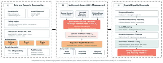
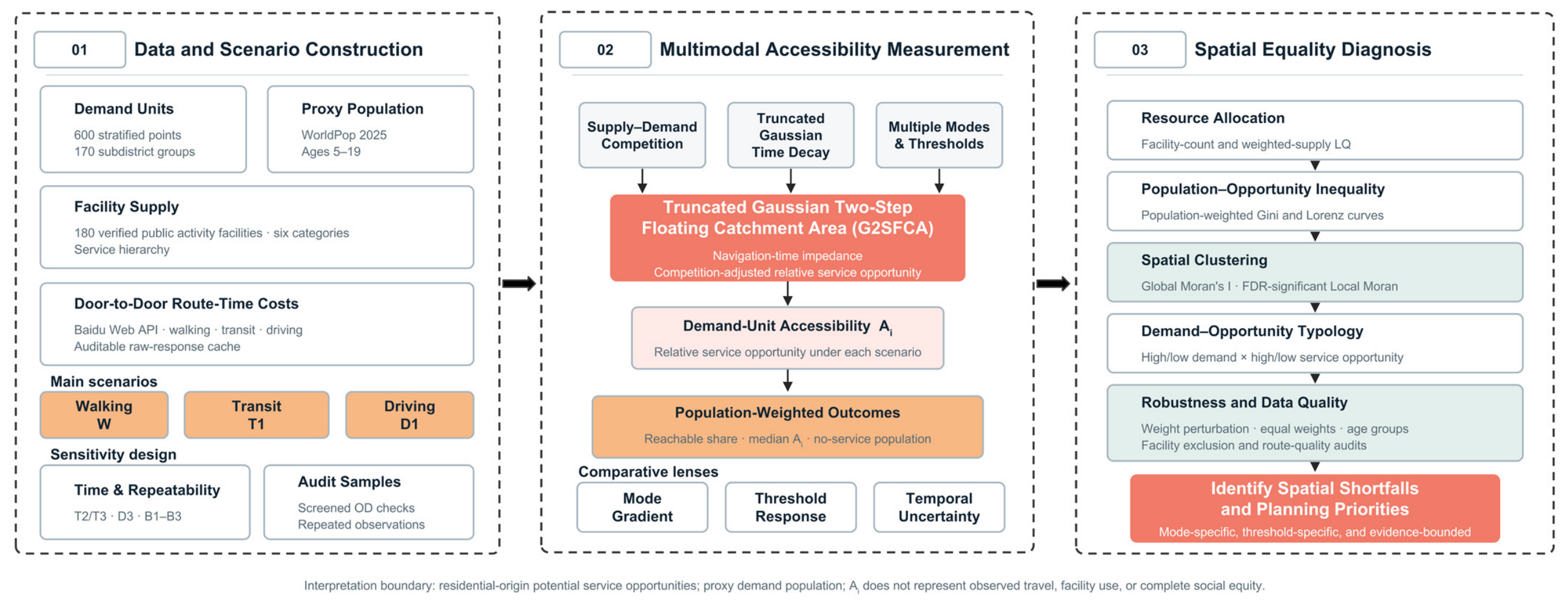
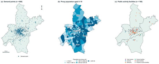
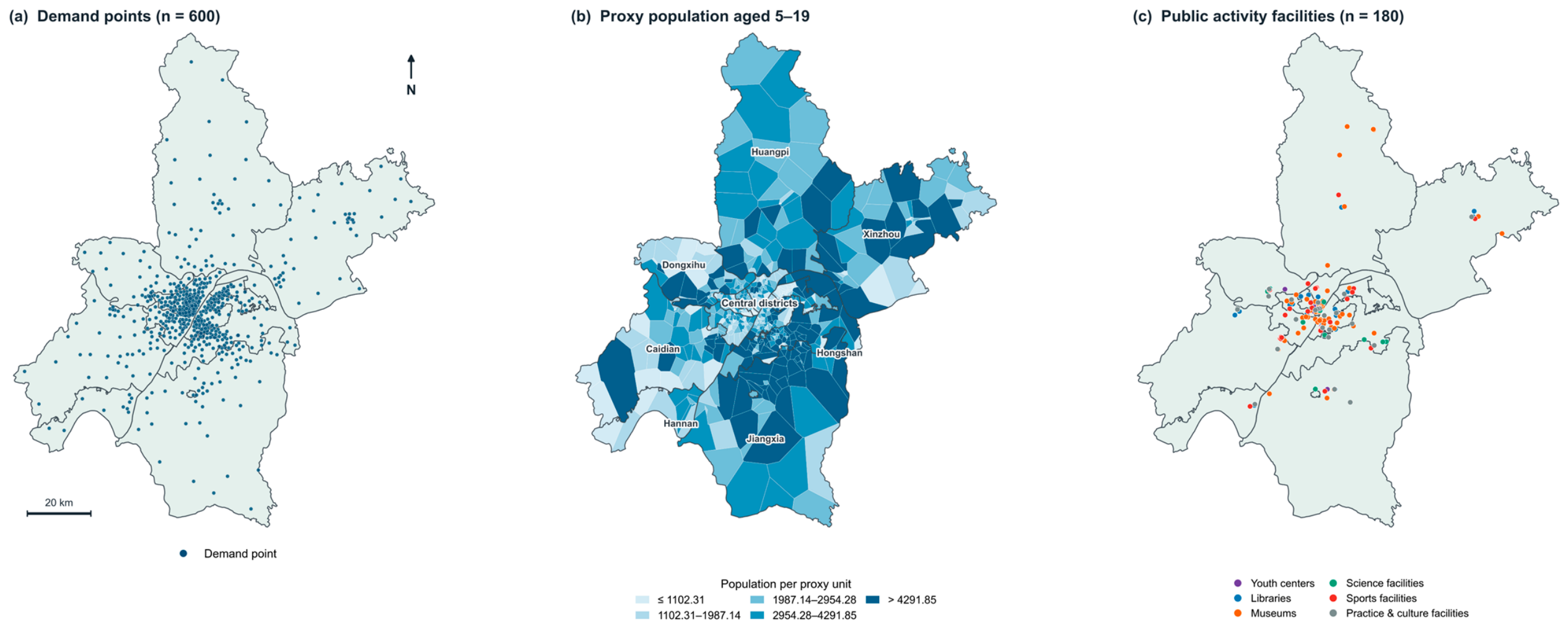
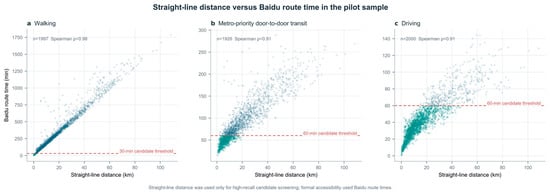
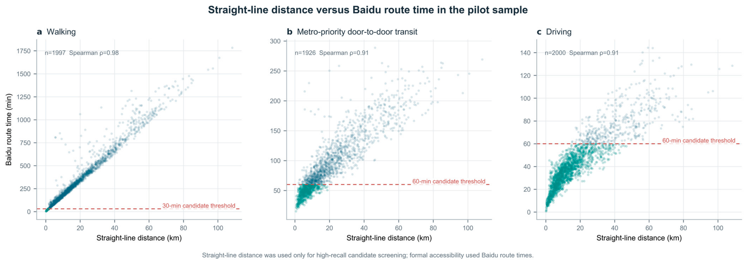
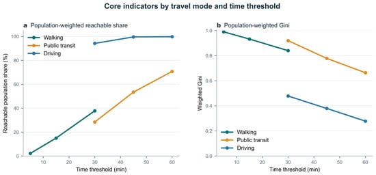
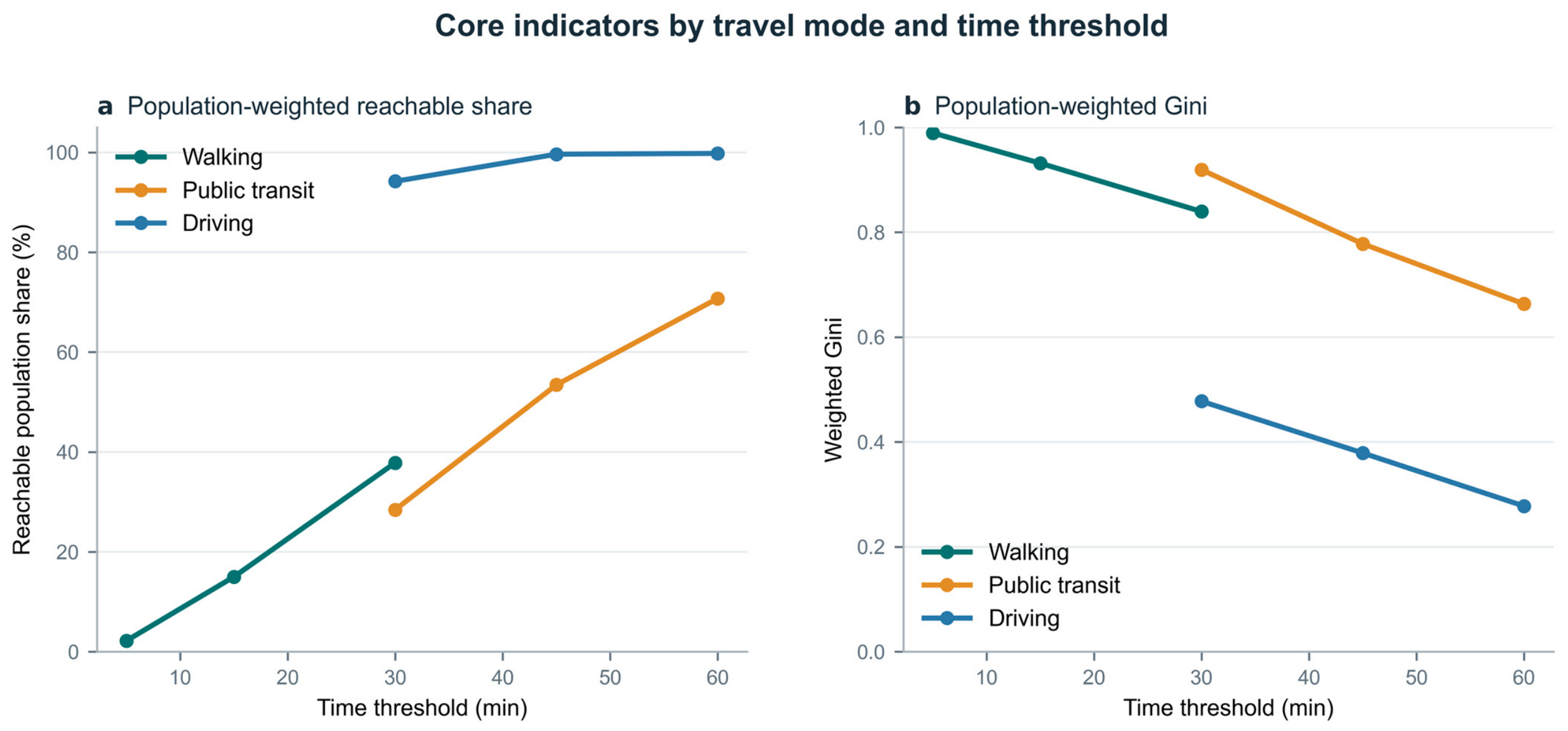
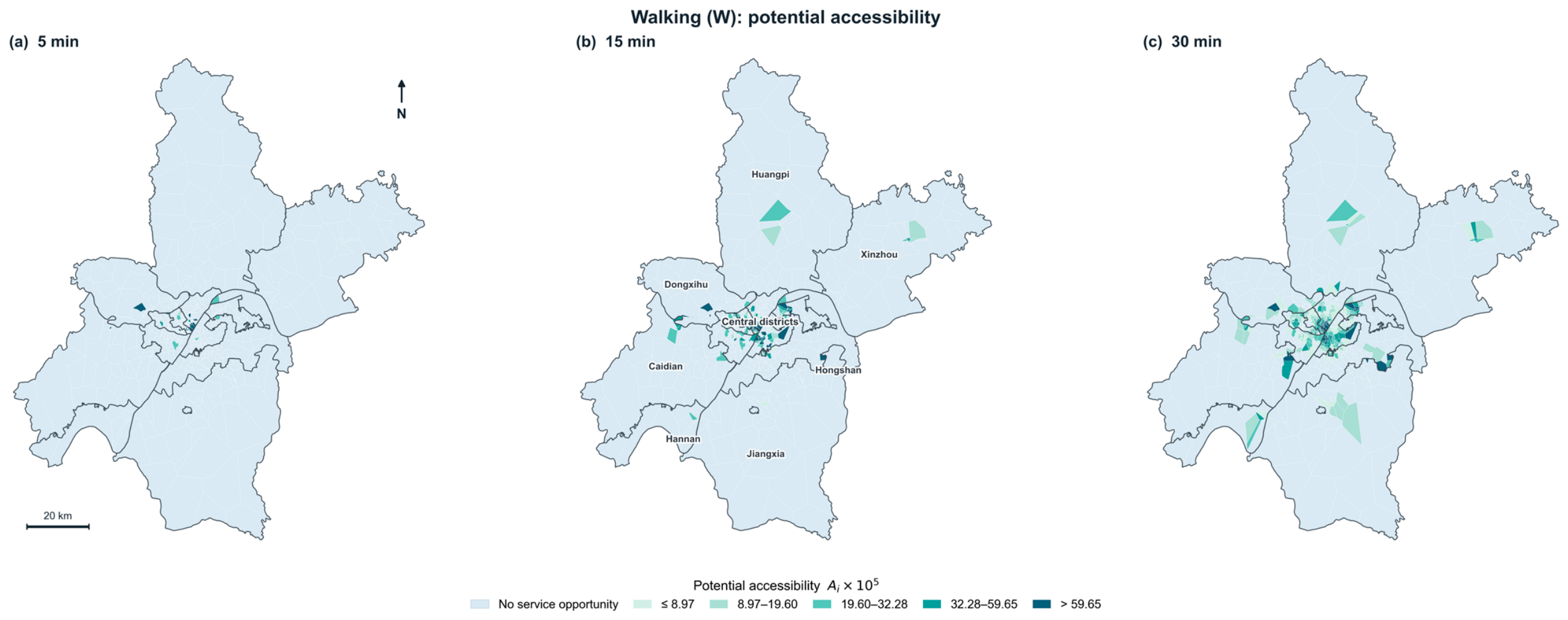
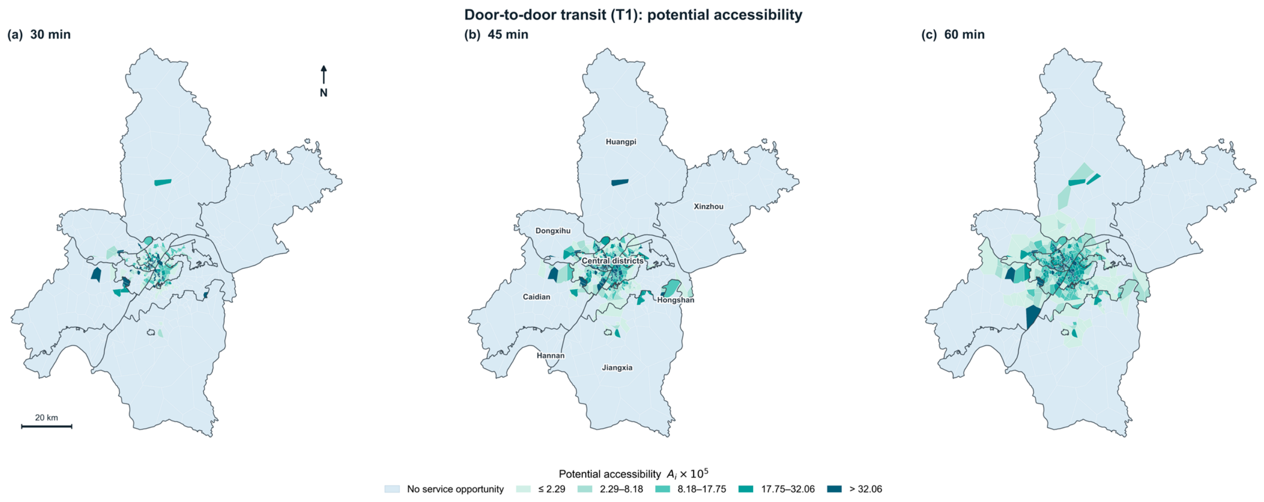
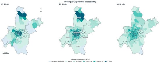
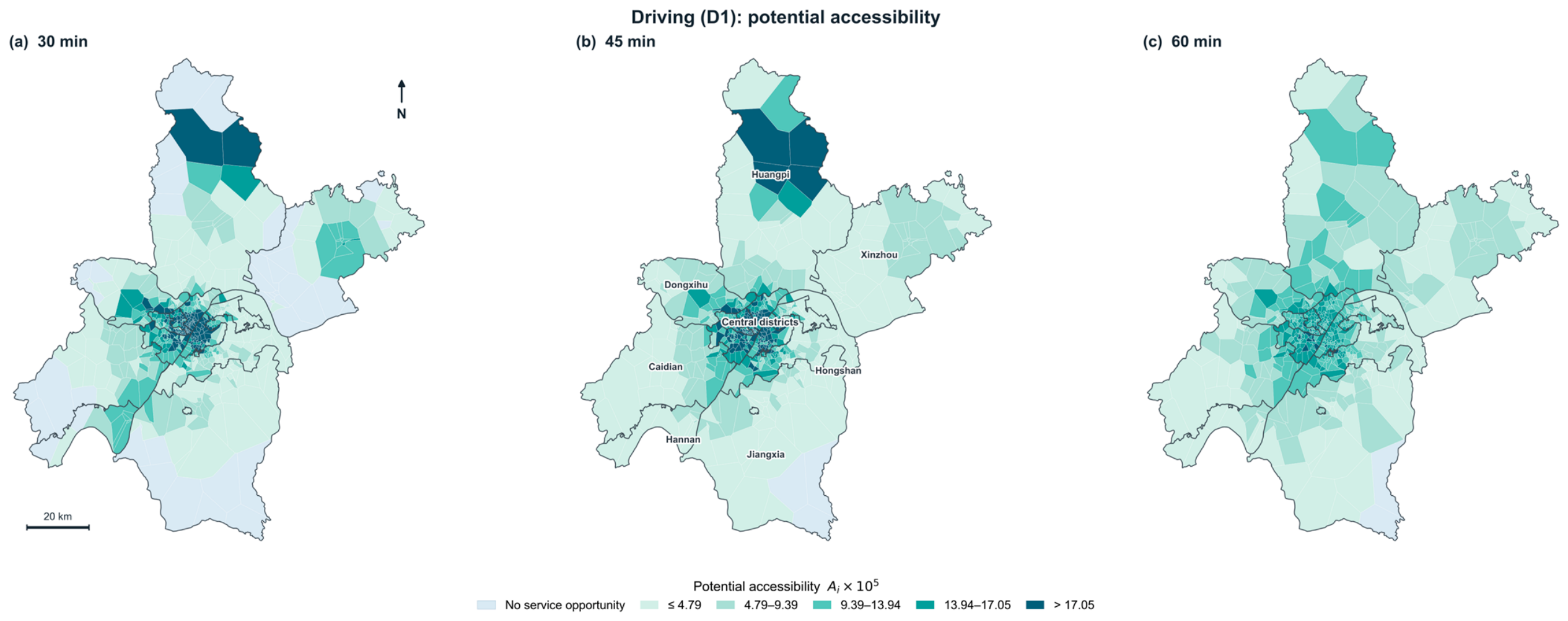
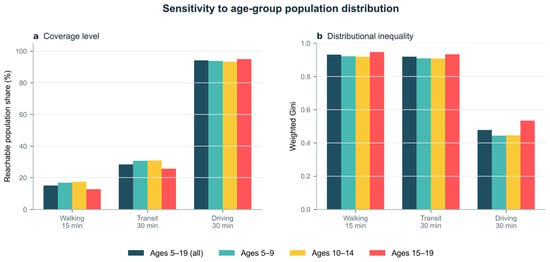
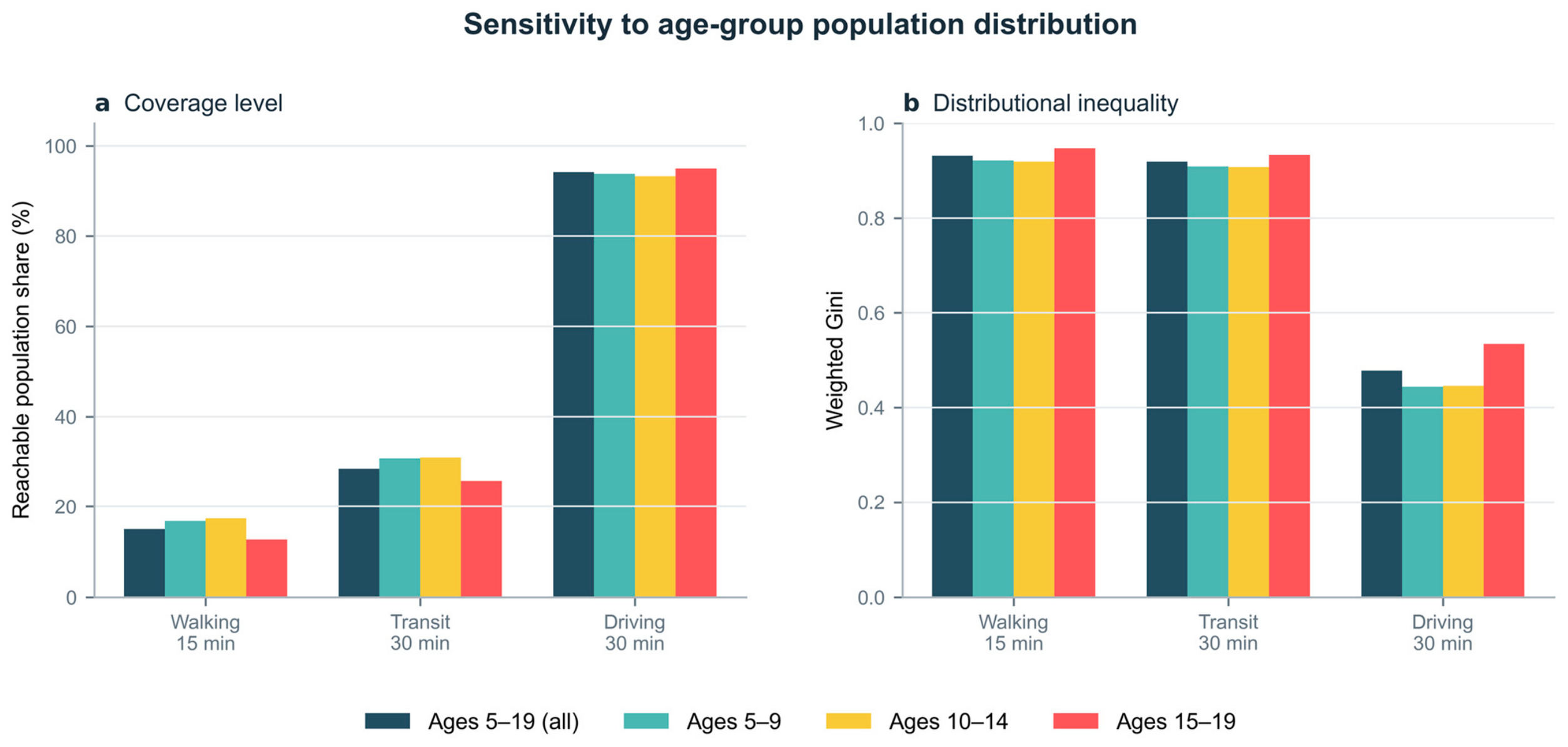
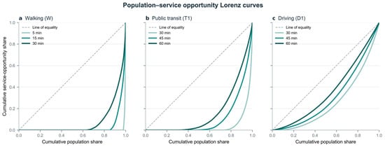
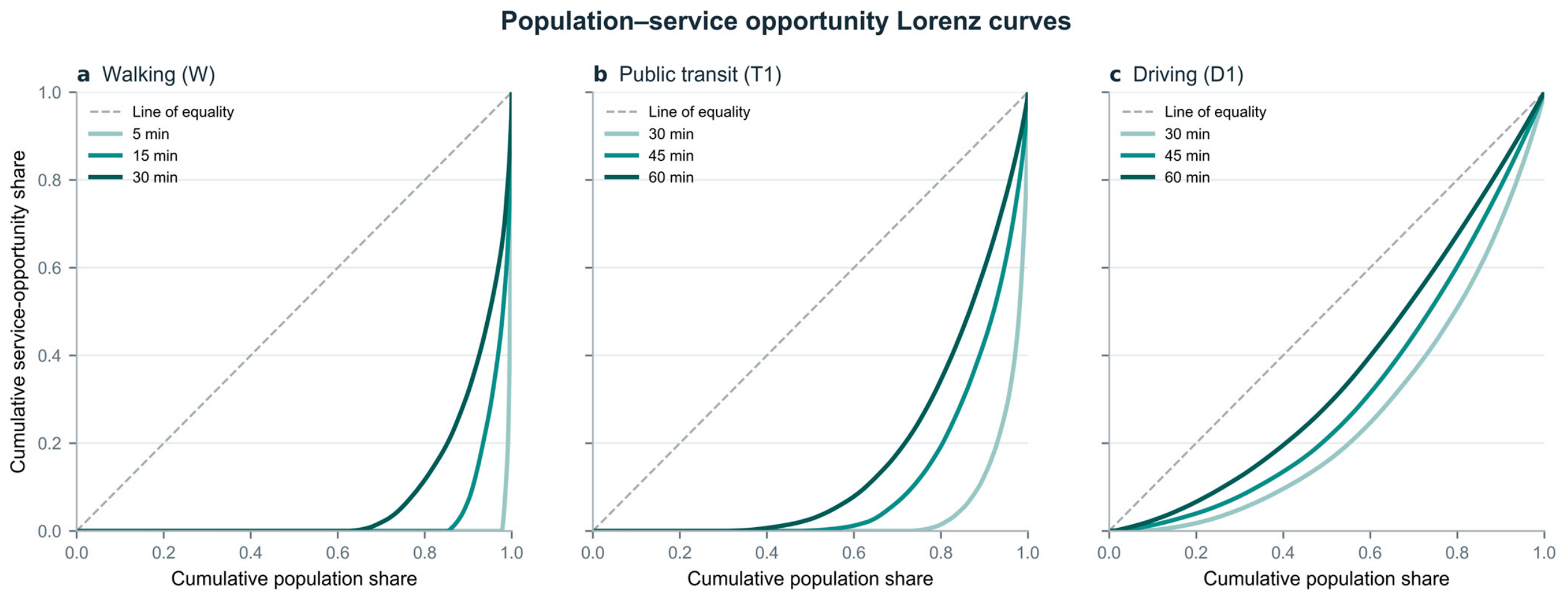
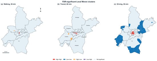
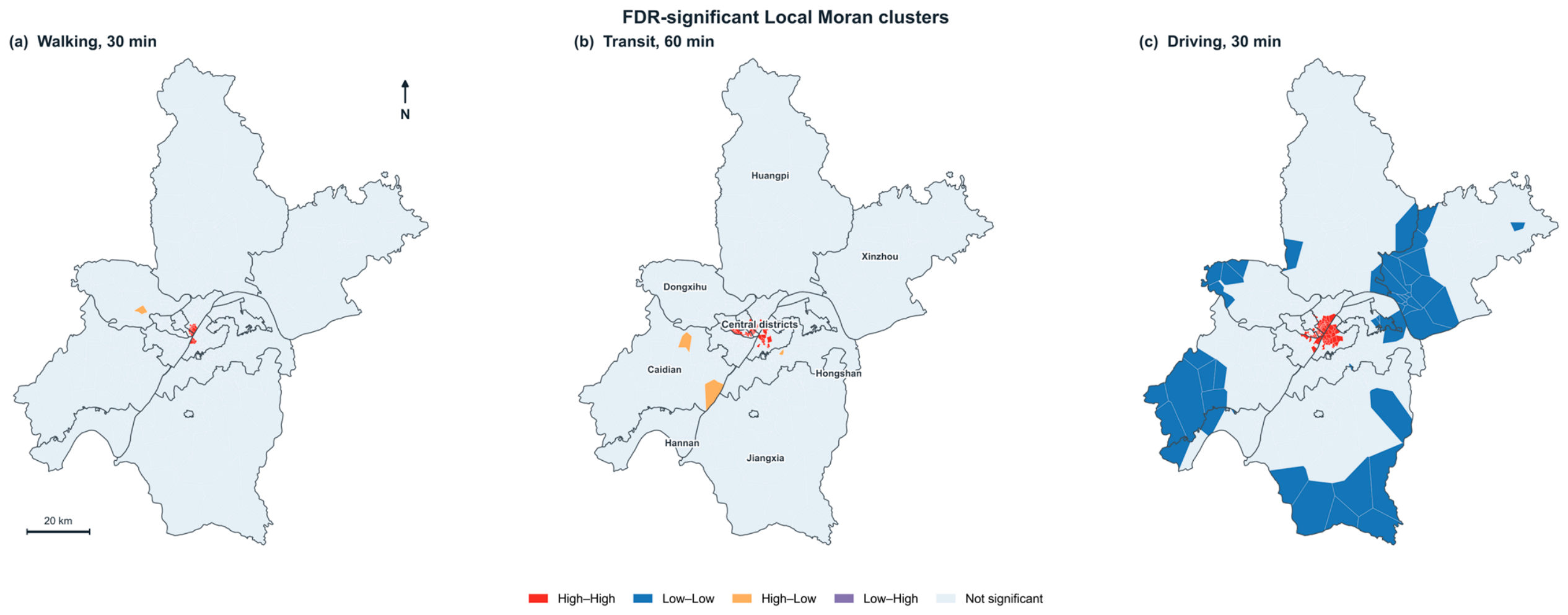
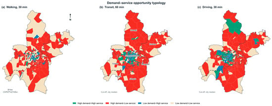
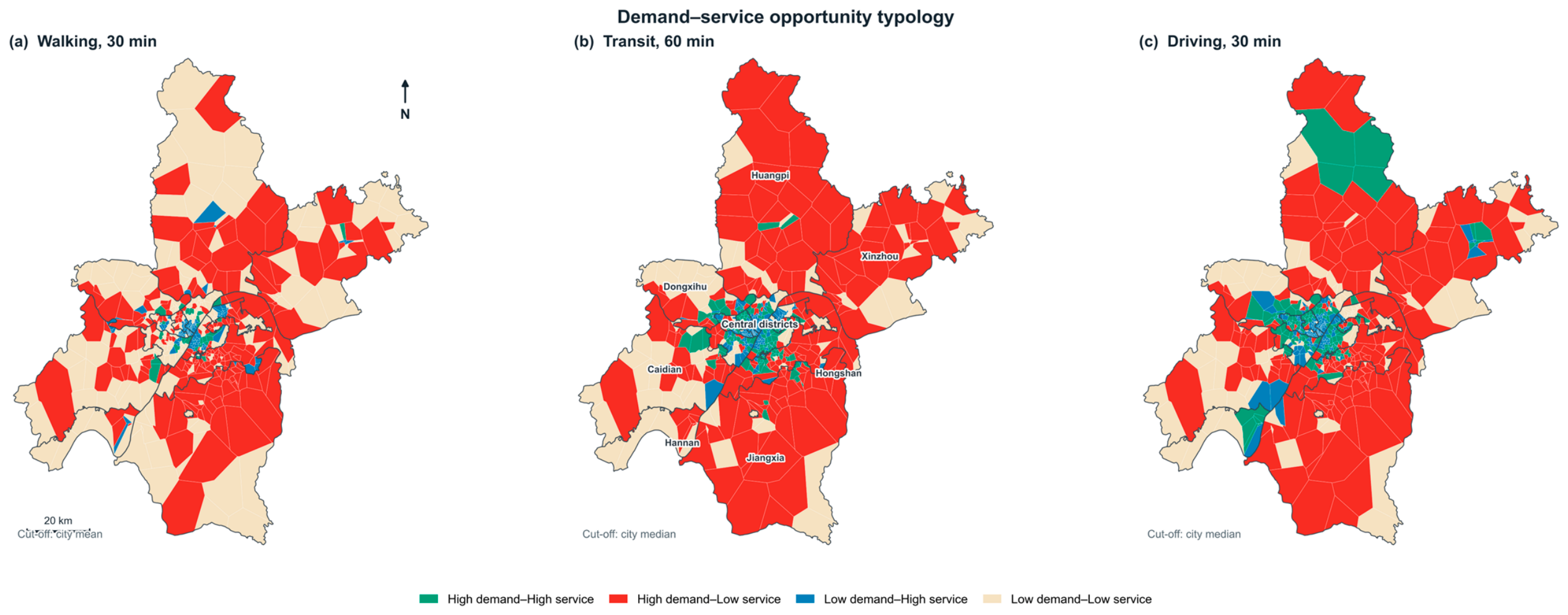
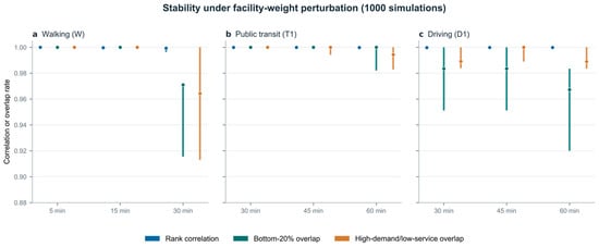
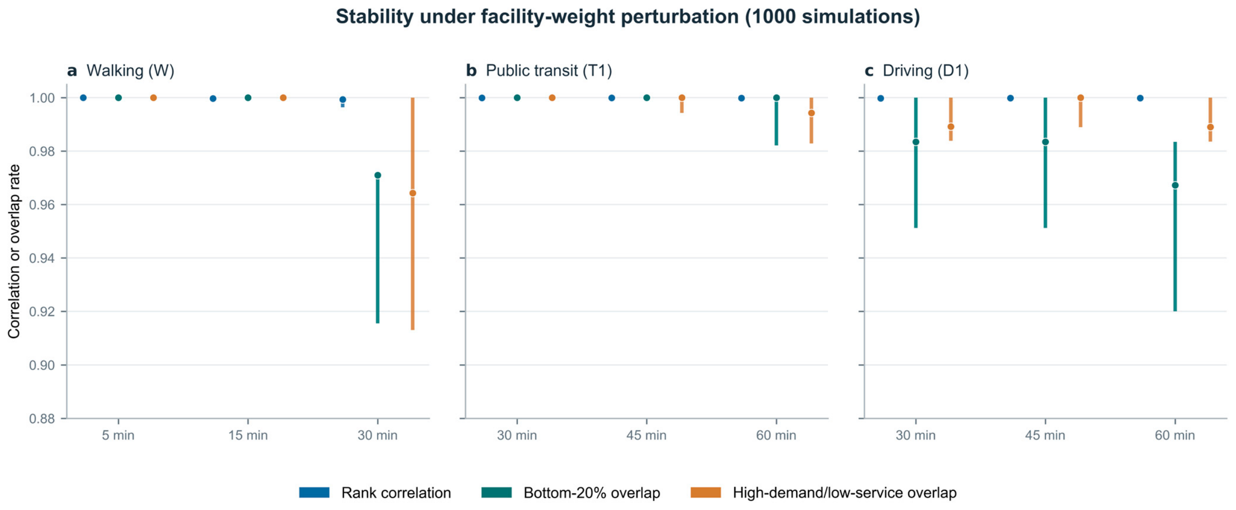
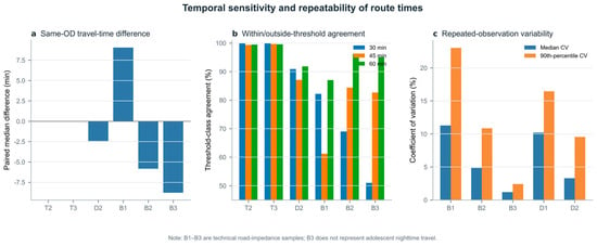
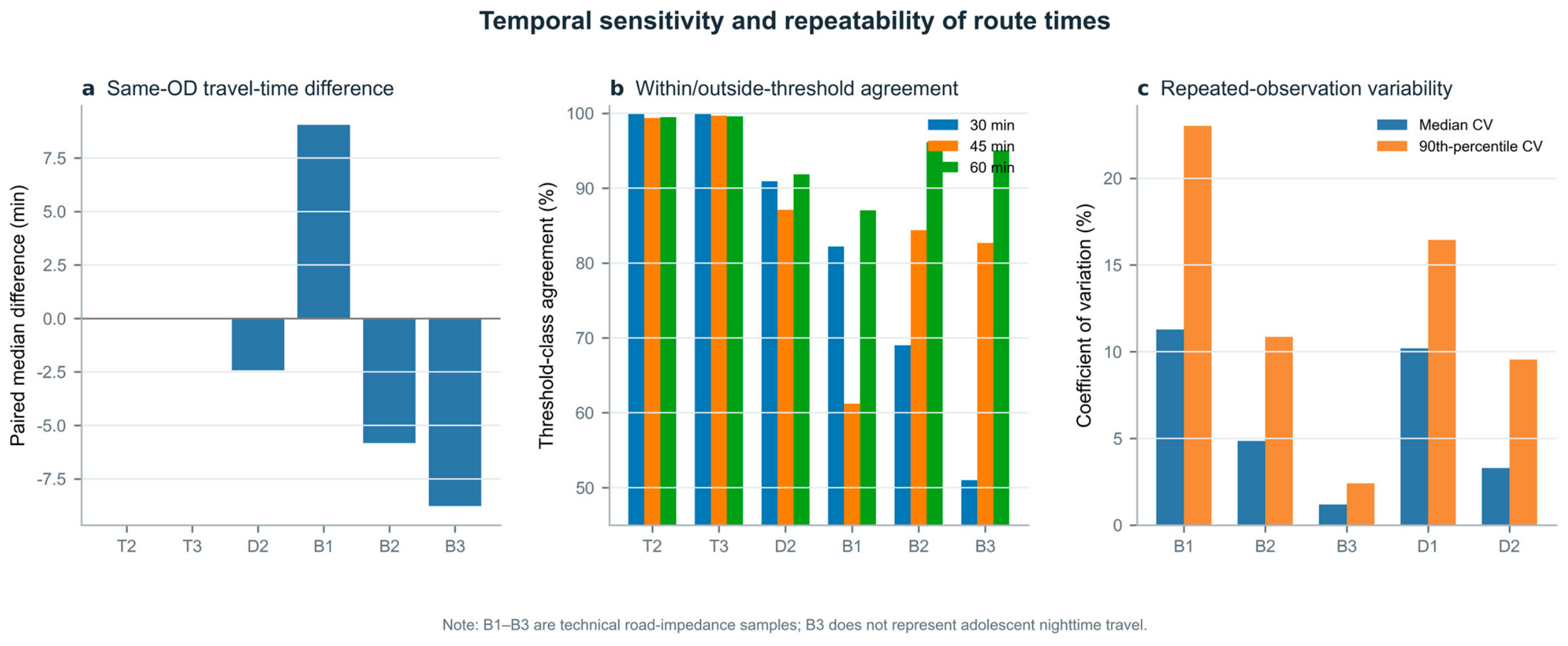

Disclaimer/Publisher’s Note: The statements, opinions and data contained in all publications are solely those of the individual author(s) and contributor(s) and not of MDPI and/or the editor(s). MDPI and/or the editor(s) disclaim responsibility for any injury to people or property resulting from any ideas, methods, instructions or products referred to in the content. |
© 2026 by the authors. Licensee MDPI, Basel, Switzerland. This article is an open access article distributed under the terms and conditions of the Creative Commons Attribution (CC BY) license.